A Hybrid Algorithm Approach to Designing a Three-Echelon Supply Chain Network Model

Abstract

This study addresses a large-scale location–allocation problem in a three-echelon automotive supply chain comprising 382 suppliers, candidate distribution centers, and six assembly plants. The planning task is to redesign the inbound consolidation network while minimizing transportation and distribution center operating costs, enforcing a 480 km supplier-to-center service radius, and achieving at least 90% demand-weighted coverage. We formulate a mixed discrete-continuous model with supplier-to-center assignment, center location, throughput, and flow decisions. A feasibility-oriented hybrid algorithm uses a genetic algorithm as the main search engine, ant colony construction to seed solutions near the feasible region, adaptive mutation and simulated annealing to preserve exploration and refine elite solutions, and an online neural surrogate to avoid a subset of costly exact fitness evaluations. The design differs from a simple collection of metaheuristics: all components share one variable-length encoding, the same feasibility metrics, and periodic exact reevaluation of candidate solutions. Using the competition case data, the redesigned network reduces total cost by 27.0% relative to the six-center baseline, decreases the demand-weighted average supplier-to-center distance from 461.3 km to 53.0 km, lowers the maximum distance from 2807.22 km to 441.78 km, and raises coverage from 45.0% to 100%. Across ten independent runs, the hybrid method obtains a mean cost 10.3% below that of a standard genetic algorithm, with lower run-to-run dispersion. The results show that feasibility-aware initialization, adaptive search, and selective surrogate evaluation can support practical redesign of a strongly constrained, national-scale inbound logistics network. The directly attached reproducibility package provides the MATLAB implementation and the seven supplied input workbooks used by the reported model. The evidence is limited to one deterministic competition instance, a fixed cost schedule, and fixed-topology sensitivity calculations; generalization under demand uncertainty, facility disruption, and alternative road conditions remains to be tested.

1. Introduction

Manufacturing supply chains increasingly rely on regional consolidation centers to coordinate geographically dispersed suppliers, stabilize inbound flows, and reduce the cost of serving multiple plants. For an automotive manufacturer, a network decision is not limited to choosing a few facility coordinates; it also determines which supplier is assigned to each center, how product demand is routed from centers to assembly plants, how much throughput each center processes, and whether the resulting service distances satisfy operational commitments. These decisions are tightly coupled: opening more centers normally raises fixed and piecewise operating costs, but it can shorten collection distances and increase the share of demand served within a prescribed radius. A national-scale instance therefore requires a method that treats cost and feasibility jointly rather than optimizing a simplified distance objective and checking service constraints only after the search.

Recent supply chain network design studies illustrate the breadth of this decision class. Fathi et al. [1] integrated location and inventory decisions under stochastic demand and lead times and developed a hybrid genetic algorithm for computational tractability. Goodarzian et al. [2] formulated a multi-period, three-echelon green medicine network and evaluated several hybrid metaheuristics. Liu et al. [3] studied a three-level location–allocation problem under distributional uncertainty and compared a hybrid intelligent algorithm with particle swarm, genetic, and decomposition-based alternatives. In a hub location setting, Demir et al. [4] showed that problem-specific mutation and neighborhood operators can materially affect the ability of evolutionary and simulated annealing methods to find high quality feasible networks; their evolutionary comparison builds on the elitist NSGA-II framework of Deb et al. [5]. Wang et al. [6] further demonstrated that third party logistics decisions can change the economics of an integrated location inventory network. Together, these studies confirm that realistic network design is both structurally rich and computationally demanding; they also show why comparisons must be made using a common representation and common feasibility rules.

A second stream of research uses learning models to reduce the cost of evaluating candidate solutions. Xiao et al. [7] proposed a machine learning-aided metaheuristic for production–distribution system design in which learned structural information supports initialization, search space restriction, and fitness approximation. Broader reviews of surrogate-assisted evolutionary optimization emphasize that a surrogate is useful only when its model management policy controls prediction error and retains sufficiently frequent exact evaluations [8,9]. This point is especially important in constrained combinatorial optimization: a low predicted objective value is not useful if the corresponding allocation violates coverage or distance requirements. Classical genetic algorithms, ant colony optimization, and simulated annealing provide complementary global, constructive, and local search mechanisms [10,11,12], but combining them does not by itself establish novelty or robustness. The components must be coordinated around the same decision encoding, constraint metrics, and acceptance logic.

The case considered here has three features that make this coordination consequential. First, 382 suppliers are distributed across mainland China and must be assigned without splitting each supplier’s outbound flow among multiple consolidation centers. Second, the number and coordinates of centers are decision variables, so the chromosome length changes with the network configuration. Third, feasibility is defined by both a 480 km maximum supplier-to-center distance and a demand-weighted coverage threshold of 90%, while operating cost changes nonlinearly with center throughput. A generic population method can spend most of its evaluations in infeasible regions or converge prematurely to a costly feasible topology. Exact evaluation of every candidate, however, is also expensive because assignments, flows, costs, and coverage must be recomputed for the full network. The research gap is therefore not the absence of hybrid algorithms in the literature; it is the need for a transparent feasibility-oriented integration that remains reproducible on a large, organizer-supplied industrial instance.

This paper makes three contributions. First, it develops a case-grounded three-echelon location–allocation model that combines linear cargo-specific transportation costs, piecewise distribution center operating costs, exclusive supplier assignment, a distance limit, and demand-weighted coverage in one objective-and-constraint system. Second, it proposes a coordinated solution architecture rather than a loose sequence of algorithms. Ant colony construction supplies feasible region information to the initial population; the genetic algorithm performs the main global search with variable-length encoding and adaptive mutation; simulated annealing refines elite solutions; and the neural surrogate is used selectively, with exact reevaluation retained for promising or constraint-sensitive candidates.

Table 1. Comparison of the implemented solution approaches and their evidentiary role.

Approach	Primary Search Role	Constraint Handling	Use in This Study	Evidence Status
Standard GA	Population-based global search	Penalty-based exact evaluator	Ten-run control	Feasible; repeated evidence
ACO	Distance-guided constructive search	Coverage-aware elite pheromone update	Initial population generator	Component of proposed method
SA	Metropolis local refinement	Uses the same penalized fitness	Elite refinement every 20 generations	Component of proposed method
PSO	Continuous swarm search over center coordinates	Generic penalty without feasibility repair	Diagnostic comparator	One run; infeasible (0% coverage)
DE	Continuous differential mutation and crossover	Generic penalty without feasibility repair	Diagnostic comparator	One run; infeasible (0% coverage)
Neural surrogate	35-input MLP fitness approximation	Prediction is periodically checked exactly	Selective evaluation accelerator	2227 predictions; final solution exact
Proposed hybrid	ACO initialization + adaptive GA + SA + MLP	One shared cost, coverage, and penalty evaluator	Primary method	Ten feasible runs plus exact reevaluation

compares the implemented solution approaches and their evidentiary roles. Third, it evaluates both managerial and computational outcomes. The case analysis separates transportation and operating cost effects, explains the large change in service distance through the network topology, and reports ten independent runs against a standard genetic algorithm. Parameter settings, surrogate usage statistics, fixed topology sensitivity results, diagnostic PSO/DE outcomes, and the directly attached code-and-data package are stated explicitly to make the claims auditable.

2. Model Description

2.1. Basic Assumptions

Regarding the optimization problem of the three-echelon supply chain network structure studied in this paper, the following assumptions are proposed:

(1) The research area is located within mainland China, where the Earth’s curvature is relatively small, and thus it can be considered a plane. The great circle distance between two points calculated by the Haversine formula ignores the influence of terrain fluctuations, road networks, and detours in reality. The distance calculation is primarily used for relative comparison rather than absolute precision.

(2) The supply capacity of all suppliers and the order demand of factories are deterministic and known, and uncertainties such as seasonal fluctuations, random disturbances, unexpected events, and force majeure are not considered during the study period.

(3) Transportation cost is represented as a linear function of route distance and cargo weight or volume, with cargo-specific coefficients. This assumption reflects the information resolution of the competition data: the organizer provides standardized conversion coefficients but does not provide shipment-level truck utilization, contract tiers, full-truckload/less-than-truckload breakpoints, or carrier-specific minimum charges. Introducing unobserved quantity discounts would therefore add parameters that cannot be calibrated consistently. The assumption should be interpreted as an aggregate planning approximation for comparing network configurations over the same study horizon, not as a detailed freight quotation model. In contrast, distribution center operating cost is piecewise because the supplied cost schedule associates throughput bands with step changes in facility resources, labor, and handling capacity. Thus, linear transportation cost and nonlinear center operating cost describe two different cost-generating mechanisms and are not internally inconsistent. A future operational model could replace the linear freight term with lane- and mode-specific tariffs when FTL/LTL and discount data become available.

(4) All goods from each supplier must be and can only be assigned to one distribution center. Splitting a single supplier’s goods for shipment to different distribution centers is not allowed.

2.2. Problem Description

Company F’s vehicle supply chain adopts the 3PL model, which means establishing the supply chain by relying on a third-party logistics enterprise. Company F has six assembly plants and 382 scattered suppliers nationwide. The distribution centers collect goods from nearby suppliers based on preset routes and schedules and then deliver them uniformly to the various assembly plants via the distribution centers. Therefore, the locations of distribution centers to be built and the supplier allocation scheme need to be determined to achieve the goal of minimizing total cost.

The 480 km threshold is treated as a service design requirement supplied with the competition case rather than as a direct proxy for weather, congestion, or road closures. Those factors can alter travel time and realized route cost, but they are not observed in the available data and are therefore outside the deterministic planning model. The model first computes comparable geographic distances for all supplier–center pairs and then measures the share of demand assigned within the prescribed radius. During the search, violations are converted into a large, graded penalty so that an infeasible candidate can still be ranked by how far it is from feasibility; a purely discontinuous rejection rule would provide little guidance to population-based operators. The penalty is therefore an algorithmic constraint-handling device, not an assertion that a carrier literally charges a weather-related surcharge whenever 480 km is exceeded. Final solutions are reported together with the actual coverage and maximum distance, and only solutions satisfying the 90% coverage requirement are treated as operationally feasible. This interpretation aligns the practical motivation with the mathematical formulation.

2.3. Sets, Parameters, and Variables

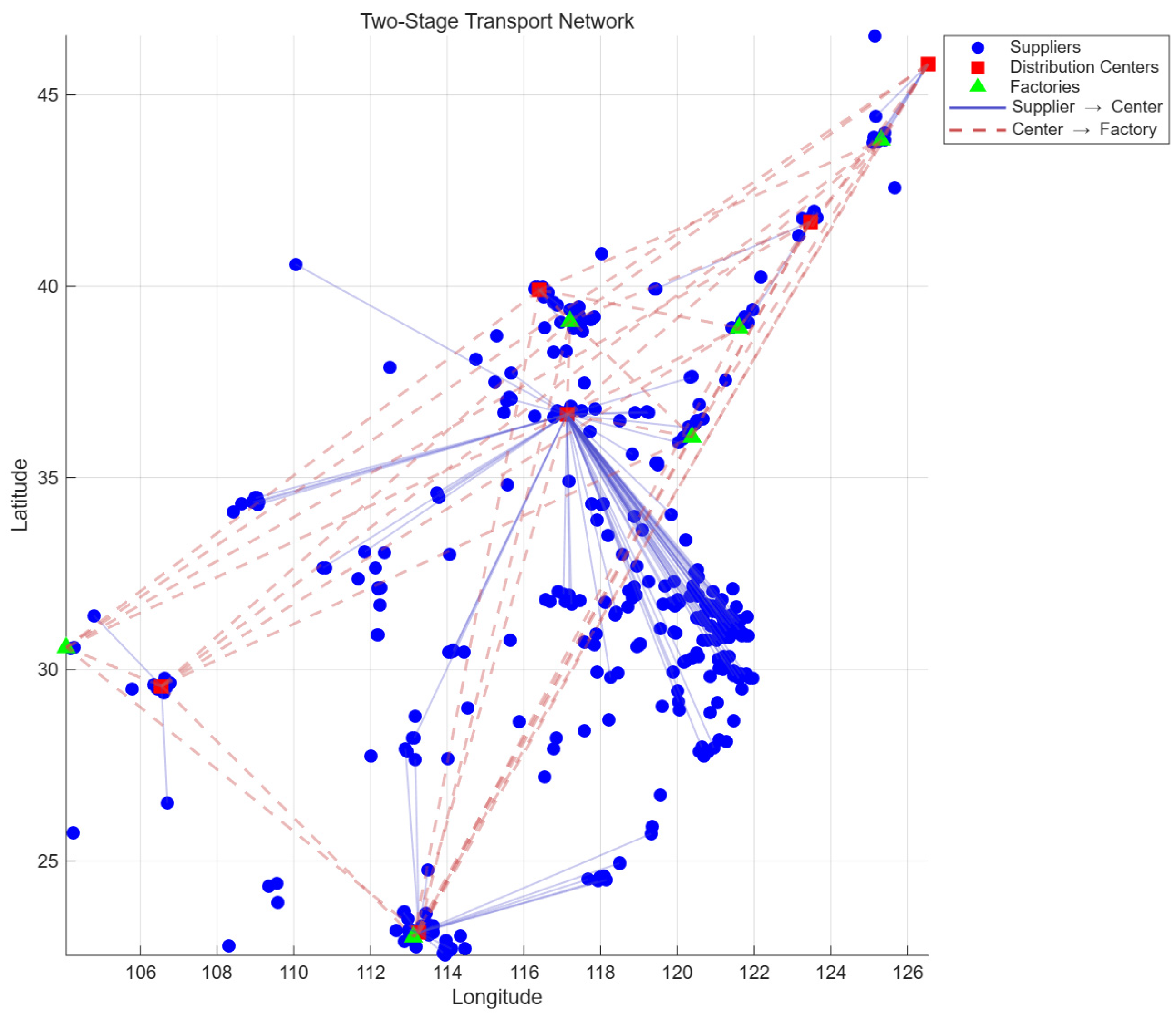
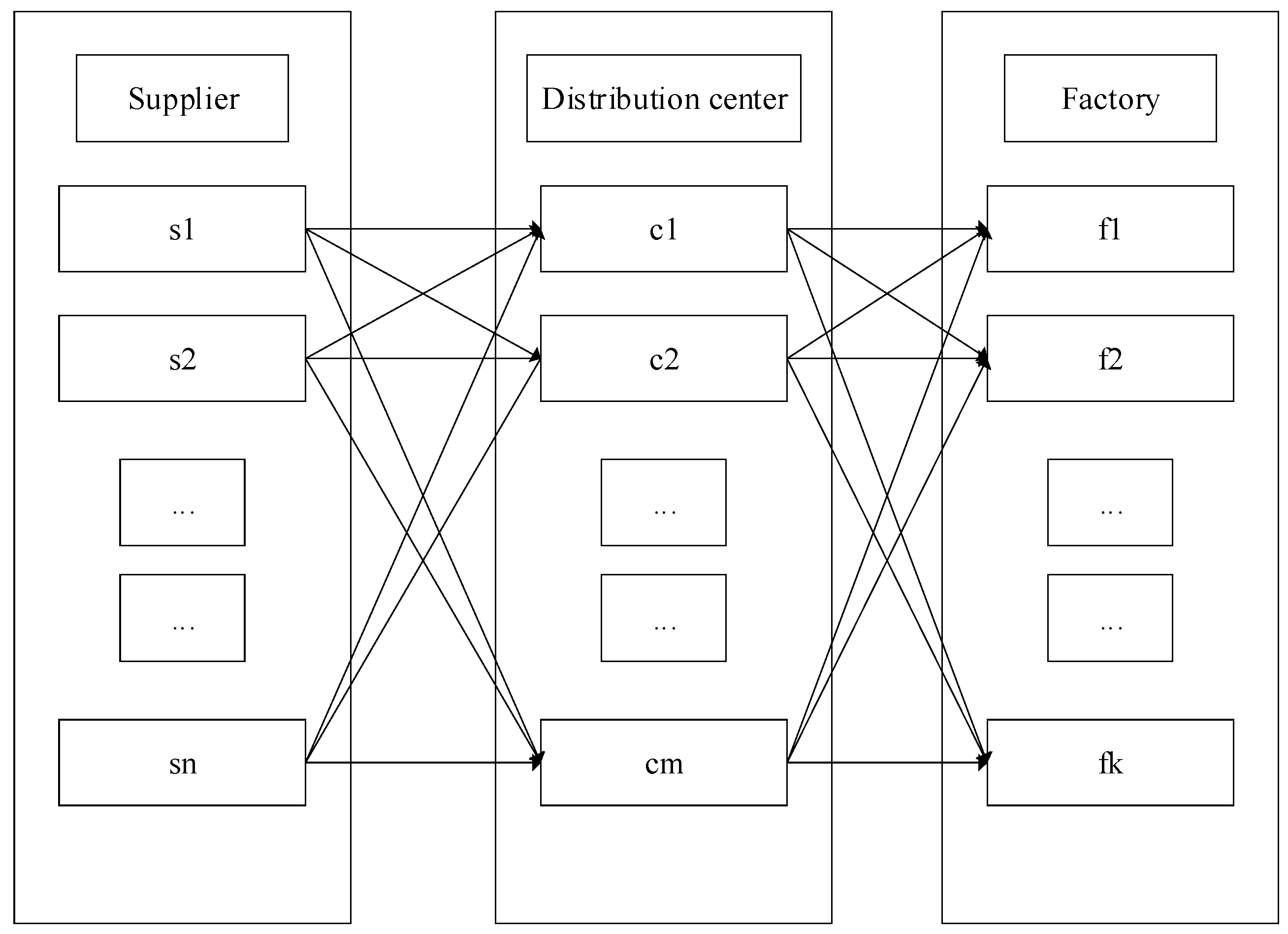
The logistics network distribution center location optimization problem is defined on a directed multigraph $\mathrm{G}=(\mathrm{V},\mathrm{A})$. Here, $\mathrm{V}$ represents the set of nodes, consisting of the supplier set S, the candidate distribution center set C, and the factory set F. To reduce model complexity, suppliers that are geographically close can be considered as the same supplier node; similarly, geographically close factories can be considered as the same factory node. $\mathrm{A}$ represents the set of arcs, including arcs from suppliers to distribution centers ${\mathrm{A}}_{\mathrm{S}\to \mathrm{C}}$ and arcs from distribution centers to factories ${\mathrm{A}}_{\mathrm{C}\to \mathrm{F}}$. However, it is noteworthy that, in real-world supply chain transportation networks, there may be multiple alternative paths connecting two points. In this model, we focus on selecting Pareto-optimal arcs, i.e., for a given path, it is impossible to improve the transportation cost of one node without increasing the transportation cost of at least one other node while satisfying all demands, ensuring efficiency and economic viability of the logistics supply chain network and avoiding resource waste under all constraints.

All transportation tasks in the supply chain network are represented by the transportation demand set $\mathrm{D}$, where each transportation demand represents the demand of a specific factory for a specific product. Transportation demands are linked to suppliers through product mapping. Therefore, let the product set be $\mathrm{P}$, and each product $\mathrm{p}\in \mathrm{P}$ corresponds to a unique supplier $\mathrm{M}\left(\mathrm{p}\right)\in$ S. Also, let $\mathrm{d}$ represent the demand of factory ${\mathrm{f}}_{\mathrm{k}}$ for product $\mathrm{p}$.

In the model, for any two nodes $\mathrm{i},\mathrm{j}\in \mathrm{V}$ in the established supply chain network, the distance between them is set as ${\mathrm{d}}_{\mathrm{i}\mathrm{j}}$, calculated using the $\mathrm{H}\mathrm{a}\mathrm{v}\mathrm{e}\mathrm{r}\mathrm{s}\mathrm{i}\mathrm{n}\mathrm{e}$ formula. In the constructed supply chain network, we only focus on two types of distances: the distance from supplier ${\mathrm{s}}_{\mathrm{i}}$ to distribution center ${\mathrm{c}}_{\mathrm{j}}$, denoted as $\mathrm{d}\left({\mathrm{s}}_{\mathrm{i}},{\mathrm{c}}_{\mathrm{j}}\right)$, and the distance from distribution center ${\mathrm{c}}_{\mathrm{j}}$ to factory ${\mathrm{f}}_{\mathrm{k}}$, denoted as $\mathrm{d}\left({\mathrm{c}}_{\mathrm{j}},{\mathrm{f}}_{\mathrm{k}}\right)$.

In the transportation network established by the model, the total transportation volume is generated by all demands. Let ${\mathrm{q}}_{\mathrm{i}}$ represent the total shipment volume from supplier ${\mathrm{s}}_{\mathrm{i}}$, which equals the sum of the demands from all factories requiring products from that supplier:

$${\mathrm{q}}_{\mathrm{i}}={\displaystyle {\sum }_{\mathrm{k}=1}^{\mathrm{p}}}{\sum }_{\mathrm{p}\in \mathrm{P}:\mathrm{M}\left(\mathrm{p}\right)={\mathrm{s}}_{\mathrm{i}}}{\mathrm{d}}_{\mathrm{k}\mathrm{p}}$$

(1)

According to the linear transportation cost assumption, transportation cost is linearly related to distance. Transporting goods the same distance incurs the same cost. In the model, distance is used as the primary calculation unit for transportation cost. Considering the throughput operation cost and construction/operation cost of distribution centers, we define ${\mathrm{C}}_1$ as the fixed construction cost of a distribution center and ${\mathrm{C}}_2$ as the operation cost of a distribution center, which is determined by a piecewise function $\mathrm{F}\mathrm{C}\left(\mathrm{q}\right)$, where $\mathrm{q}$ is the throughput of the distribution center.

Define the following decision variables:

$${\mathrm{x}}_{\mathrm{j}}=\left\{\begin{array}{c}1,\mathrm{i}\mathrm{f} \mathrm{a} \mathrm{d}\mathrm{i}\mathrm{s}\mathrm{t}\mathrm{r}\mathrm{i}\mathrm{b}\mathrm{u}\mathrm{t}\mathrm{i}\mathrm{o}\mathrm{n} \mathrm{c}\mathrm{e}\mathrm{n}\mathrm{t}\mathrm{e}\mathrm{r} \mathrm{i}\mathrm{s} \mathrm{b}\mathrm{u}\mathrm{i}\mathrm{l}\mathrm{t} \mathrm{a}\mathrm{t} \mathrm{n}\mathrm{o}\mathrm{d}\mathrm{e} \mathrm{j} \\ 0, \mathrm{o}\mathrm{t}\mathrm{h}\mathrm{e}\mathrm{r}\mathrm{w}\mathrm{i}\mathrm{s}\mathrm{e} \end{array}\mathrm{j}\in \mathrm{C}\right.$$

(2)

$$y_{ij}=1 if s_i is assigned{c}_j; 0 otherwise, i \in S, j \in C$$

(3)

Distribution center throughput decision variable ${\mathrm{t}}_{\mathrm{j}},\mathrm{j}\in \mathrm{C}$ represents the total cargo volume (units) processed by distribution center ${\mathrm{c}}_{\mathrm{j}}$. Transportation variable ${\mathrm{z}}_{\mathrm{j}\mathrm{k}},\mathrm{j}\in \mathrm{C},\mathrm{k}\in \mathrm{F}$ represents the shipment volume (units) from distribution center ${\mathrm{c}}_{\mathrm{j}}$ to factory ${\mathrm{f}}_{\mathrm{k}}$. Distance violation variable ${\mathsf{\delta }}_{\mathrm{i}\mathrm{j}},\mathrm{i}\in \mathrm{S},\mathrm{j}\in \mathrm{C}$ represents the excess of the actual distance from supplier i to distribution center j over the allowed maximum distance:

$${\mathsf{\delta }}_{\mathrm{i}\mathrm{j}}=\mathrm{m}\mathrm{a}\mathrm{x}\left(0,\mathrm{d}\left({\mathrm{s}}_{\mathrm{i}},{\mathrm{c}}_{\mathrm{j}}\right)\right)-{\mathrm{D}}_{\mathrm{m}\mathrm{a}\mathrm{x}})$$

(4)

Coverage variable $\mathrm{r}$ represents the proportion of transportation volume satisfying the distance constraint relative to the total transportation volume.

Based on the above, the symbols and variable definitions for this model are shown in

Table 2. Definition of model symbols and variables.

Type	Symbol	Definition
Sets	$S$	Supplier node set, $\mathrm{S}=\{{\mathrm{s}}_1,{\mathrm{s}}_2,\dots ,{\mathrm{s}}_{\mathrm{n}}\}$
	$C$	Candidate distribution center node set, $\mathrm{C}=\{{\mathrm{c}}_1,{\mathrm{c}}_2,\dots ,{\mathrm{c}}_{\mathrm{m}}\}$
	$F$	Factory node set, $\mathrm{F}=\{{\mathrm{f}}_1,{\mathrm{f}}_2,\dots ,{\mathrm{f}}_{\mathrm{k}}\}$
	$P$	Product set, $\mathrm{P}=\{{\mathrm{p}}_1,{\mathrm{p}}_2,\dots ,{\mathrm{p}}_{\mathrm{l}}\}$
	$V$	All nodes set, $\mathrm{V}=\mathrm{S}\cup \mathrm{C}\cup \mathrm{F}$
	$T$	Cargo type set, $\mathrm{T}=\{\mathrm{h}\mathrm{e}\mathrm{a}\mathrm{v}\mathrm{y} \mathrm{c}\mathrm{a}\mathrm{r}\mathrm{g}\mathrm{o}, \mathrm{v}\mathrm{o}\mathrm{l}\mathrm{u}\mathrm{m}\mathrm{e}\mathrm{t}\mathrm{r}\mathrm{i}\mathrm{c} \mathrm{c}\mathrm{a}\mathrm{r}\mathrm{g}\mathrm{o},$ $\mathrm{h}\mathrm{a}\mathrm{z}\mathrm{a}\mathrm{r}\mathrm{d}\mathrm{o}\mathrm{u}\mathrm{s} \mathrm{m}\mathrm{a}\mathrm{t}\mathrm{e}\mathrm{r}\mathrm{i}\mathrm{a}\mathrm{l}, \mathrm{f}\mathrm{r}\mathrm{a}\mathrm{g}\mathrm{i}\mathrm{l}\mathrm{e} \mathrm{g}\mathrm{o}\mathrm{o}\mathrm{d}\mathrm{s}\}$
Parameters	$d_{ij}$	Distance (km) from node $\mathrm{i}$ to node $\mathrm{j}$
	$d_{ij}^S$	Distance from supplier ${\mathrm{s}}_{\mathrm{i}}$ to distribution center ${\mathrm{c}}_{\mathrm{j}}$, ${\mathrm{d}}_{\mathrm{i}\mathrm{j}}^{\mathrm{S}}=\mathrm{d}({\mathrm{s}}_{\mathrm{i}},{\mathrm{c}}_{\mathrm{j}})$
	$d_{jk}^F$	Distance from distribution center ${\mathrm{c}}_{\mathrm{j}}$ to factory ${\mathrm{f}}_{\mathrm{k}}$, ${\mathrm{d}}_{\mathrm{j}\mathrm{k}}^{\mathrm{F}}=\mathrm{d}({\mathrm{c}}_{\mathrm{j}},{\mathrm{f}}_{\mathrm{k}})$
	$w_i$	Unit weight (ton/unit) of goods from supplier ${\mathrm{s}}_{\mathrm{i}}$
	$v_i$	Unit volume (m3/unit) of goods from supplier ${\mathrm{s}}_{\mathrm{i}}$
	$t_i$	Cargo type of supplier ${\mathrm{s}}_{\mathrm{i}}$’s goods, ${\mathrm{t}}_{\mathrm{i}}\in \mathrm{T}$
	$\alpha \left(t\right)$	First-stage transportation cost coefficient, related to cargo type ${\mathrm{t}}_{\mathrm{i}}$
	$\beta \left(t\right)$	Second-stage transportation cost coefficient, related to cargo type ${\mathrm{t}}_{\mathrm{i}}$
	$D_{max}$	Maximum allowable transportation distance, ${\mathrm{D}}_{\mathrm{m}\mathrm{a}\mathrm{x}}=480\mathrm{k}\mathrm{m}$
	$R_{min}$	Minimum coverage requirement, ${\mathrm{R}}_{\mathrm{m}\mathrm{i}\mathrm{n}}=0.90$
	$\lambda$	Constraint violation penalty coefficient
	$d_{kp}$	Demand quantity (units) of factory ${\mathrm{f}}_{\mathrm{k}}$ for product $\mathrm{p}$
	$M\left(p\right)$	Product supplier mapping function
	$q_i$	Total supply from supplier ${\mathrm{s}}_{\mathrm{i}}$
	$Q$	Total demand quantity
	$FC\left(q\right)$	Distribution center operation cost function, a piecewise function of throughput $\mathrm{q}$ (yuan)
	$C_1$	Fixed construction cost of a distribution center (yuan)
	$C_2$	Distribution center operation cost
Variables	$x_j$	Whether to build a distribution center at node $\mathrm{j}$
	$y_{ij}$	Whether supplier ${\mathrm{s}}_{\mathrm{i}}$ is assigned to distribution center ${\mathrm{c}}_{\mathrm{j}}$
	$z_{jk}$	Shipment volume from distribution center ${\mathrm{c}}_{\mathrm{j}}$ to factory ${\mathrm{f}}_{\mathrm{k}}$
	$t_j$	Throughput of distribution center ${\mathrm{c}}_{\mathrm{j}}$
	$v_{ij}$	Distance violation indicator variable
	$r$	Actual coverage rate

.

2.4. Objective Function and Constraints

$$minZ=TC+OC+PC$$

(5)

$$TC=T{C}_1+T{C}_2$$

(6)

$$T{C}_1={\displaystyle \sum _{i=1}^n}{\displaystyle \sum _{j=1}^m}\alpha \left(t_i\right)·C_i·d\left(s_i,c_j\right)·y_{ij}·D_i$$

(7)

$$T{C}_2={\displaystyle \sum _{j=1}^m}{\displaystyle \sum _{k=1}^p}\beta \left(t\right)·C_j·d\left(c_j,f_k\right)·z_{jk}$$

(8)

$$OC={\displaystyle {\sum }_{j=1}^m}{x}_j·FC\left(t_j\right)$$

(9)

$$FC\left(t_j\right)=\left\{\begin{array}{cc}\mathrm{12,000,000},\hfill & \hfill 0\le t_j\le \mathrm{300,000}\\ \mathrm{12,000,000},\hfill & \hfill \mathrm{300,000}\le t_j\le \mathrm{600,000}\\ \mathrm{16,000,000},\hfill & \hfill \mathrm{600,000}\le t_j\le \mathrm{900,000}\\ \mathrm{19,500,000},\hfill & \hfill \mathrm{900,000}\le t_j\le \mathrm{1,200,000}\\ \mathrm{22,500,000},\hfill & \hfill \mathrm{1,200,000}\le t_j\le \mathrm{1,500,000}\\ \mathrm{25,000,000},\hfill & \hfill t_i>\mathrm{1,500,000}\end{array}\right.$$

(10)

$$PC=\lambda ·\mathit{max}\left(0,R_{min}-r\right)+\lambda ·{\displaystyle \frac{{\sum }_{i=1}^n{\sum }_{j=1}^m{v}_{ij}}{n·m}}$$

(11)

$${\displaystyle {\sum }_{j=1}^m}{y}_{ij}=1, \forall i=\mathrm{1,2},\dots ,n$$

(12)

$$y_{ij}\le x_j, \forall i=\mathrm{1,2},\dots ,n, j=\mathrm{1,2},\dots ,m$$

(13)

$${\displaystyle {\sum }_{i=1}^n}{y}_{ij}·D_i={\displaystyle {\sum }_{k=1}^p}{z}_{jk}, \forall j=\mathrm{1,2},\dots ,m$$

(14)

$$t_j={\sum }_{i=1}^n{y}_{ij}·D_i, \forall i=\mathrm{1,2},\dots ,n$$

(15)

$$v_{ij}\ge {\displaystyle \frac{d\left(s_i,c_i\right)-D_{max}}{M}}+y_{ij}-1,\forall i=\mathrm{1,2},\dots ,n, j=\mathrm{1,2},\dots ,m$$

(16)

$$v_{ij}\le y_{ij}, \forall i=\mathrm{1,2},\dots ,n, j=\mathrm{1,2},\dots ,m$$

(17)

$$v_{ij}\le {\displaystyle \frac{d\left(s_i,c_j\right)-D_{max}}{M}}+1,\forall i=\mathrm{1,2},\dots ,n, j=\mathrm{1,2},\dots ,m$$

(18)

$$r={\displaystyle \frac{{\sum }_{i=1}^n{\sum }_{j=1}^m{y}_{ij}·\left(1-v_{ij}\right)·D_i}{Q}}$$

(19)

$$Q={\sum }_{i=1}^n{D}_i$$

(20)

$$r\ge R_{min}$$

(21)

$$z_{jk}\ge 0, \forall j=\mathrm{1,2},\dots ,m,k=\mathrm{1,2},\dots ,p$$

(22)

$$t_j\ge 0, \forall j=\mathrm{1,2},\dots ,m$$

(23)

$$x_j\in \left\{\mathrm{0,1}\right\}, \forall j=\mathrm{1,2},\dots ,m$$

(24)

$$y_{ij}\in \left\{\mathrm{0,1}\right\}, \forall i=\mathrm{1,2},\dots ,n, j=\mathrm{1,2},\dots ,m$$

(25)

$$v_{ij}\in \left\{\mathrm{0,1}\right\}, \forall i=\mathrm{1,2},\dots ,n, j=\mathrm{1,2},\dots ,m$$

(26)

$$0\le r\le 1$$

(27)

$$d\left(s_i,c_j\right)=d\left(c_j,s_i\right),\forall i=\mathrm{1,2},\dots ,n, j=\mathrm{1,2},\dots ,m$$

(28)

$$\left(s_i,f_k\right)\le d\left(s_i,c_j\right)+d\left(c_j,f_k\right),\forall i=\mathrm{1,2},\dots ,n, j=\mathrm{1,2},\dots ,m,k=\mathrm{1,2},\dots ,p$$

(29)

$$\alpha \left(t_i\right)=\left\{\begin{array}{c}0.68, { t}_i=heavy cargo\\ 0.33, { t}_i=volumetric cargo\\ 0.82, t_i=hazardous material\\ 1.02, t_i=fragile goods\\ 0.68, { t}_i=other\end{array}\right.$$

(30)

$$\beta \left(t_i\right)=\left\{\begin{array}{c}0.44, t_i=heavy cargo\\ 0.21, t_i=volumetric cargo \\ 0.63, t_i=hazardous material\\ 0.98, t_i=fragile goods\\ 0.44, t_i=other\end{array}\right.$$

(31)

$$d\left(i,j\right)=\mathit{arcsin}\left(\sqrt{{\mathit{sin}}^2\left({\displaystyle \frac{\Delta lat}{2}}\right)+\mathit{cos}\left(la{t}_i\right)\mathit{cos}\left(la{t}_j\right){\mathit{sin}}^2\left({\displaystyle \frac{\Delta lon}{2}}\right)}\right)$$

(32)

$$\lambda =1\times {10}^{12}$$

(33)

The objective function (5) indicates minimizing the total cost, which consists of three parts: total transportation cost, total operation cost, and total penalty cost. The total transportation cost $\mathrm{T}\mathrm{C}$ includes two parts: the first-stage transportation cost $\mathrm{T}{\mathrm{C}}_1$ from suppliers to distribution centers and the second-stage transportation cost $\mathrm{T}{\mathrm{C}}_2$ from distribution centers to factories. Specific calculation formulas are given in Equations (7) and (8). The relationship between the transportation cost coefficients $\mathsf{\alpha }\left({\mathrm{t}}_{\mathrm{i}}\right)$ and $\mathsf{\beta }\left({\mathrm{t}}_{\mathrm{i}}\right)$ and the cargo type ${\mathrm{t}}_{\mathrm{i}}$ is shown in Equations (30) and (31). The total operation cost $\mathrm{O}\mathrm{C}$ is calculated as in Equation (9), where $\mathrm{F}\mathrm{C}\left({\mathrm{t}}_{\mathrm{j}}\right)$ is the distribution center operation cost function, with its specific piecewise form given in Equation (10). The throughput of a distribution center is defined as the sum of supplies from all suppliers assigned to that center, calculated as in Equation (15). The penalty cost $\mathrm{P}\mathrm{C}$ is calculated as in Equation (11), and Equation (33) defines the value of $\mathsf{\lambda }$.

Equations (12)–(22) are the constraint equations. Equation (12) ensures each supplier must be assigned to exactly one distribution center. Equation (13) states that only selected distribution centers can receive suppliers. To ensure flow balance, we define the flow balance constraint (14), requiring the total cargo received by each distribution center to equal the total cargo it ships to all factories. Equations (16)–(18) are linearized definitions for the distance violation indicator variable ${\mathrm{v}}_{\mathrm{i}\mathrm{j}}$. The actual coverage rate $\mathrm{r}$ is defined as the proportion of cargo transportation volume satisfying the distance constraint to the total transportation volume, calculated by Equation (19). Equation (20) calculates the total demand $\mathrm{Q}$. Equation (21) is the requirement for the actual coverage rate target. Equations (22) and (23) are non-negativity constraints for continuous decision variables. Equations (24)–(27) are constraints on the types of decision variables. Equations (28) and (29) are distance symmetry and triangle inequality constraints, where the distance $\mathrm{d}\left(\mathrm{i},\mathrm{j}\right)$ between two points is calculated by the $\mathrm{H}\mathrm{a}\mathrm{v}\mathrm{e}\mathrm{r}\mathrm{s}\mathrm{i}\mathrm{n}\mathrm{e}$ formula in Equation (32).

3. Model Solving

The logistics network distribution center location optimization problem is an NP-hard problem. This problem simultaneously considers location, supplier allocation, distance constraints, coverage constraints, and operation costs, making it a complex combinatorial optimization problem. Traditional exact algorithms struggle to solve large-scale problems within a reasonable time. This paper designs a hybrid intelligent optimization algorithm that integrates the global exploration capability of the ant colony algorithm, the population evolution capability of the genetic algorithm, the evaluation acceleration capability of a deep learning model, and the local fine-tuning search capability of the simulated annealing algorithm. The algorithm framework is primarily based on a genetic algorithm, embedding an ant colony algorithm to generate initial populations, utilizing a deep learning model to predict fitness for accelerated evaluation, and employing simulated annealing for local optimization. Additionally, strategies based on elite preservation and diversity maintenance are designed to improve the algorithm’s search capability.

3.1. Solution Representation and Fitness Function

Any solution $\mathrm{x}$ contains two parts of information: the number of distribution centers and their locations. A variable-length chromosome encoding is used:

$$\mathrm{x}=[\mathrm{n},{\mathrm{l}\mathrm{a}\mathrm{t}}_1,{\mathrm{l}\mathrm{o}\mathrm{n}}_1,{\mathrm{l}\mathrm{a}\mathrm{t}}_2,{\mathrm{l}\mathrm{o}\mathrm{n}}_2,\dots ,{\mathrm{l}\mathrm{a}\mathrm{t}}_{\mathrm{n}},{\mathrm{l}\mathrm{o}\mathrm{n}}_{\mathrm{n}}]$$

(34)

where $\mathrm{n}$ is the number of distribution centers, $1\le \mathrm{n}\le {\mathrm{m}}_{\mathrm{m}\mathrm{a}\mathrm{x}}$, with ${\mathrm{m}}_{\mathrm{m}\mathrm{a}\mathrm{x}}$ being the maximum allowed number of centers; and $(\mathrm{l}\mathrm{a}\mathrm{t}\mathrm{ₖ},\mathrm{l}\mathrm{o}\mathrm{n}\mathrm{ₖ})$ are the latitude and longitude coordinates of the k-th distribution center. Each coordinate must satisfy boundary constraints:

$${\mathrm{l}\mathrm{a}\mathrm{t}}_{\mathrm{m}\mathrm{i}\mathrm{n}}\le \mathrm{l}\mathrm{a}\mathrm{t}\mathrm{ₖ}\le {\mathrm{l}\mathrm{a}\mathrm{t}}_{\mathrm{m}\mathrm{a}\mathrm{x}},\mathrm{l}\mathrm{o}\mathrm{n}\_\mathrm{m}\mathrm{i}\mathrm{n}\le \mathrm{l}\mathrm{o}\mathrm{n}\mathrm{ₖ}\le \mathrm{l}\mathrm{o}\mathrm{n}\_\mathrm{m}\mathrm{a}\mathrm{x}$$

(35)

To handle constraints, distance constraints and coverage constraints are integrated into the objective function through a penalty function. The fitness function is defined as

$$\mathrm{f}\left(\mathrm{x}\right)={\displaystyle \frac{1}{\left(\mathrm{Z}\right(\mathrm{x})+1)}}$$

(36)

where $\mathrm{Z}\left(\mathrm{x}\right)=\mathrm{T}\mathrm{C}\left(\mathrm{x}\right)+\mathrm{O}\mathrm{C}\left(\mathrm{x}\right)+\mathrm{P}\mathrm{C}\left(\mathrm{x}\right)$ is the total cost, $\mathrm{T}\mathrm{C}\left(\mathrm{x}\right)$ is the transportation cost, $\mathrm{O}\mathrm{C}\left(\mathrm{x}\right)$ is the operation cost, and $\mathrm{P}\mathrm{C}\left(\mathrm{x}\right)$ is the penalty cost. The operation cost $\mathrm{O}\mathrm{C}\left(\mathrm{x}\right)$ includes the fixed construction cost ${\mathrm{C}}_1$ and the operation cost ${\mathrm{C}}_2$ of distribution centers.

3.2. Generation of Initial Solutions

A high quality initial population can accelerate algorithm convergence. This paper employs an ant colony algorithm to generate the initial population, leveraging the pheromone positive feedback mechanism of the ant colony algorithm to produce a set of well-distributed, high quality initial solutions within the solution space.

The steps for generating initial solutions based on the ant colony algorithm are as follows:

Step 1: Initialize the pheromone matrix $\mathsf{\tau }$ and the heuristic information matrix $\mathsf{\eta }$. The initial pheromone value is set to ${\mathsf{\tau }}_0$. The heuristic information ${\mathsf{\eta }}_{\mathrm{i}\mathrm{j}}$ is calculated based on the distance between suppliers and candidate centers, with smaller distances yielding larger heuristic values.

Step 2: Set the number of ants Nants. Each ant independently constructs a solution. Each ant randomly selects a number $\mathrm{n}$ from 1 to the maximum number of centers ${\mathrm{m}}_{\mathrm{m}\mathrm{a}\mathrm{x}}$ as the number of centers for that solution.

Step 3: Ants select center locations. Each ant selects $\mathrm{n}$ center locations with probabilities determined jointly by pheromone and heuristic information.

Step 4: Evaluate the solution constructed by each ant and calculate its fitness. Update the pheromone based on fitness:

$${\mathsf{\tau }}_{\mathrm{i}\mathrm{j}}=\left(1-\mathsf{\rho }\right){\mathsf{\tau }}_{\mathrm{i}\mathrm{j}}+\Delta {\mathsf{\tau }}_{\mathrm{i}\mathrm{j}}$$

(37)

where $\mathsf{\rho }$ is the pheromone evaporation coefficient and $\Delta {\mathsf{\tau }}_{\mathrm{i}\mathrm{j}}$ is the pheromone increment, proportional to the quality of the solution.

Step 5: Repeat Steps 2–4 until the preset number of iterations is reached, then output ${\mathrm{N}}_{\mathrm{p}\mathrm{o}\mathrm{p}}$ relatively good solutions as the initial population for the genetic algorithm. The pseudo-code of the ACO-based initial population generation is given in Algorithm 1.

Algorithm 1. Feasibility-aware ACO initialization
Input	Supplier/factory coordinates, population size 120, 150 ants, 60 ACO iterations, alpha = 1.2, beta = 2.5, rho = 0.15, Q = 150.
1:	For each supplier candidate i do
2:	Set pheromone taui:= 0.1
3:	Compute normalized distance-based heuristic etai
4:	end for
5:	for iteration = 1 to 60 do
6:	for each ant = 1 to 150 do
7:	Sample a center count
8:	Select center candidates with probability proportional to taualpha × etabeta
9:	Encode the variable-length chromosome
10:	Evaluate total cost,480 km demand-weighted coverage, and penalty with the shared exact evaluator
11:	end for
12:	Evaporate pheromone by (1 − rho)
13:	Rank solutions, prioritize candidates with coverage ≥ 0.90
14:	Deposit Q times fitness (doubled for feasible candidates)
15:	Retain the best distinct candidates
16:	if fewer than 120 are available then
17:	Add bounded random candidates and exact-evaluate them
18:	end if
19:	end for
20:	return the 120-solution initial population and its exact fitness/constraint records
Output	A 120-solution initial population and its exact fitness/constraint records for the GA.

3.3. Crossover, Mutation, and Neighborhood Operator Operations

3.3.1. Crossover Operator Operation

In this algorithm model, a combination of uniform crossover and arithmetic crossover is used.

Step 1: Extract the number of centers ${\mathrm{n}}_1$ and ${\mathrm{n}}_2$ from parents ${\mathrm{P}}_1$ and ${\mathrm{P}}_2$, respectively. The offspring’s number of centers ${\mathrm{n}}_{\mathrm{c}}$ is the average of the two (rounded):

$${\mathrm{n}}_{\mathrm{c}}=[{\displaystyle \frac{{\mathrm{n}}_1+{\mathrm{n}}_2}{2}}+0.5]$$

(38)

Step 2: For the first $\min \left({\mathrm{n}}_1,{\mathrm{n}}_2,{\mathrm{n}}_{\mathrm{c}}\right)$ centers, use uniform crossover, inheriting center coordinates from parent ${\mathrm{P}}_1$ or ${\mathrm{P}}_2$ with a probability of 0.5 each.

Step 3: If ${\mathrm{n}}_{\mathrm{c}}>\min \left({\mathrm{n}}_1,{\mathrm{n}}_2,{\mathrm{n}}_{\mathrm{c}}\right)$, randomly generate positions for the new additional centers, ensuring they are within the boundary limits.

Step 4: If ${\mathrm{n}}_{\mathrm{c}}<\mathrm{m}\mathrm{i}\mathrm{n}({\mathrm{n}}_1,{\mathrm{n}}_2,{\mathrm{n}}_{\mathrm{c}})$, discard the excess center position operators.

3.3.2. Mutation Operator Operations

This model mainly sets three different mutation operations, executed with different probabilities.

• Center Number Mutation

This mutation method increases or decreases the number of centers by one within the coordinate range with probability ${\mathrm{p}}_{\mathrm{m}1}$. Increasing a center adds a randomly generated center coordinate to the end of the solution vector; decreasing a center randomly removes a center and modifies/compresses the solution vector.

2.

Position Mutation

This mutation method applies Gaussian perturbation to a randomly selected center coordinate with probability ${\mathrm{p}}_{\mathrm{m}2}$:

$${\mathrm{l}\mathrm{a}\mathrm{t}}_{\mathrm{k}}^{\prime }={\mathrm{l}\mathrm{a}\mathrm{t}}_{\mathrm{k}}+\mathsf{{\rm N}}(0,{\mathsf{\sigma }}_{\mathrm{l}\mathrm{a}\mathrm{t}}^2)$$

(39)

$${\mathrm{l}\mathrm{o}\mathrm{n}}_{\mathrm{k}}^{\prime }={\mathrm{l}\mathrm{o}\mathrm{n}}_{\mathrm{k}}+\mathsf{{\rm N}}(0,{\mathsf{\sigma }}_{\mathrm{l}\mathrm{o}\mathrm{n}}^2)$$

(40)

where $\mathsf{\sigma }$ gradually decreases as the number of iterations increases, achieving adaptive mutation.

3.

Center Replacement

This mutation method replaces one center with another randomly generated center with probability ${\mathrm{p}}_{\mathrm{m}3}$, thereby increasing population diversity.

3.3.3. Neighborhood Operations

For neighborhood operations, this algorithm primarily uses the simulated annealing optimization algorithm for local optimization, executed on elite individuals in the population every K generations. The simulated annealing uses the following neighborhood operations:

• Center Position Fine-tuning:

Randomly select a center and apply a small random perturbation to its latitude and longitude. The perturbation amplitude decreases as the temperature lowers.

2.

Center Merging:

If the distance between two centers is too close, defined as less than the merge threshold ${\mathrm{d}}_{\mathrm{m}\mathrm{e}\mathrm{r}\mathrm{g}\mathrm{e}}$, merge them into one center. The new position is the weighted average, with weights being the number of suppliers assigned to each center.

3.

Center Splitting:

If the throughput of a certain center is too large, exceeding the split threshold ${\mathrm{q}}_{\mathrm{s}\mathrm{p}\mathrm{l}\mathrm{i}\mathrm{t}}$, split it into two centers. The new center positions are randomly generated around the original center.

The simulated annealing optimization algorithm’s acceptance criterion uses the Metropolis criterion:

$$\mathrm{P}(\mathrm{a}\mathrm{c}\mathrm{c}\mathrm{e}\mathrm{p}\mathrm{t})=\mathrm{m}\mathrm{i}\mathrm{n}(1,\mathrm{e}\mathrm{x}\mathrm{p}({\displaystyle \frac{\mathrm{f}\left({\mathrm{x}}_{\mathrm{n}\mathrm{e}\mathrm{w}}\right)-\mathrm{f}\left({\mathrm{x}}_{\mathrm{c}\mathrm{u}\mathrm{r}\mathrm{r}\mathrm{e}\mathrm{n}\mathrm{t}}\right)}{\mathrm{T}}}))$$

(41)

Temperature decreases according to a geometric cooling schedule: ${\mathrm{T}}_{\mathrm{k}+1}=\mathsf{\alpha }{\mathrm{T}}_{\mathrm{k}}$.

The complete genetic algorithm main loop is summarized in Algorithm 2.

Algorithm 2. Adaptive genetic search.
Input	ACO population; population = 120; generations ≤ 400; initial crossover = 0.85; initial mutation = 0.30; elite count = 8.
1:	For generation g = 1 to max_generations do
2:	Compute recent mean coverage.
3:	if mean coverage is below 0.85 then
4:	raise mutation to at most 0.45
5:	else
6:	decay mutation toward 0.05
7:	end if
8:	if generation g is within the first 40% of generations then
9:	keep crossover at 0.85
10:	else
11:	set crossover to 0.7225
12:	end if
13:	Select parents by roulette sampling while copying the best feasible elites unchanged.
14:	Apply variable-length crossover and center-count/coordinate mutation.
15:	Enforce latitude, longitude, and center-count bounds.
16:	Use exact evaluation early.
17:	Later permit the neural fitness estimate only under the staged verification policy.
18:	Every 20 generations, send the top 10% of individuals to Algorithm 3.
19:	Accept an SA result only if its exact fitness improves.
20:	Retain the historical best solution.
21:	if generation limit reached or stagnation condition met then
22:	break
23:	end if
24:	end for
25:	return Best chromosome, cost/coverage history, active center topology, and exact final metrics.
Output	A 120-solution initial population and its exact fitness/constraint records for the GA.

Algorithm 3. Simulated-annealing refinement of an elite solution.
Input	Elite chromosome x; T0 = 100; final temperature = 0.1; cooling factor = 0.98; maximum local iterations = 50.
1:	Set current = best = x
2:	Exact-evaluate current fitness with the shared constraint evaluator
3:	Set T = T0
4:	Set iter = 0
5:	while T > 0.1 and iter < 50 do
6:	Generate a bounded neighbor using center relocation and structure-changing neighborhood opera tions
7:	Exact-evaluate the neighbor
8:	if neighbor fitness improves then
9:	Accept neighbor as new current
10:	else
11:	Accept neighbor with probability exp((f_new − f_current)/T)
12:	end if
13:	if accepted solution improves the local best then
14:	Update best record
15:	end if
16:	Set T = 0.98 * T
17:	iter = iter + 1
18:	end while
19:	return refined chromosome and exact fitness
Output	Refined chromosome and exact fitness; the GA replaces its elite only when this fitness is better.

3.4. Deep Learning Neural Network Fitness Evaluation

The implemented deep-learning component is a multilayer perceptron (MLP) regressor that predicts the scalar fitness of one encoded network solution. It is not a convolutional, recurrent, or generative model, and it does not directly choose distribution center locations. Its only role is to approximate selected fitness evaluations inside the evolutionary search; exact cost and feasibility evaluation remains authoritative for verified candidates and the final solution.

3.4.1. Feature Extraction

To accurately predict the fitness of a solution, features that comprehensively reflect its quality need to be extracted from the solution $\mathrm{x}$. These features should cover multiple dimensions of the solution, including structural features, spatial distribution features, constraint satisfaction features, and interaction features with the network topology.

3.4.2. Model Architecture

The supplied MATLAB2025A implementation instantiates a 35-128-64-32-1 feedforward regression network: a 35-value input, three fully connected hidden layers with 128, 64, and 32 units, and one linear scalar output. Each hidden block uses batch normalization, ReLU activation, and dropout at 0.20. The feature routine allocates 25 engineered slots, populates 21 with center-count, spatial dispersion, approximate coverage, distance, cargo, factory, and demand summaries, and pads reserved slots to the 35-value network input. This padding is reported explicitly because the model architecture is fixed at 35 inputs even though not every reserved feature is active in the supplied version.

The input layer receives the 35-value feature vector described above. Features are computed from the candidate chromosome and case parameters; no image, text, or time-series input is used. The output is a bounded fitness estimate in [0, 1], consistent with the implementation of fitness as 1/(1 + penalized cost).

The first hidden layer is a fully connected layer containing 128 neurons. The output of each neuron is calculated as follows:

$${\mathrm{h}}_{\mathrm{j}}^{\left(1\right)}=\mathrm{f}\left({\displaystyle {\sum }_{\mathrm{i}=1}^{\mathrm{d}}}{\mathrm{w}}_{\mathrm{j}\mathrm{i}}^{\left(1\right)}{\mathsf{\varphi }}_{\mathrm{i}}\left(\mathrm{x}\right)+{\mathrm{b}}_{\mathrm{j}}^{\left(1\right)}\right),\mathrm{j}=\mathrm{1,2},\dots \dots ,128$$

(42)

where ${\mathrm{w}}_{\mathrm{j}\mathrm{i}}^{\left(1\right)}$ is the connection weight from the i-th neuron of the input layer to the j-th neuron of the first hidden layer, ${\mathrm{b}}_{\mathrm{j}}^{\left(1\right)}$ is the bias term, and $\mathrm{f}$ is the activation function.

The second hidden layer is a fully connected layer containing 64 neurons. Its input is the output of the first hidden layer, and its output is calculated as:

$${\mathrm{h}}_{\mathrm{k}}^{\left(2\right)}=\mathrm{f}\left({\displaystyle {\sum }_{\mathrm{j}=1}^{128}}{\mathrm{w}}_{\mathrm{k}\mathrm{j}}^{\left(2\right)}{\mathrm{h}}_{\mathrm{j}}^{\left(1\right)}+{\mathrm{b}}_{\mathrm{k}}^{\left(2\right)}\right),\mathrm{k}=\mathrm{1,2},\dots \dots ,64$$

(43)

The third hidden layer contains 32 neurons and uses the same fully connected, ReLU, and dropout sequence. Its output is

$${\mathrm{h}}_{\mathrm{l}}^{\left(3\right)}=\mathrm{f}\left({\displaystyle {\sum }_{\mathrm{k}=1}^{64}}{\mathrm{w}}_{\mathrm{l}\mathrm{k}}^{\left(3\right)}{\mathrm{h}}_{\mathrm{k}}^{\left(2\right)}+{\mathrm{b}}_{\mathrm{l}}^{\left(3\right)}\right),\mathrm{l}=\mathrm{1,2},\dots \dots ,32$$

(44)

The output layer is a single-neuron fully connected layer used to output the predicted fitness value:

$$\widehat{\mathrm{f}}\left(\mathrm{x}\right)={\displaystyle {\sum }_{\mathrm{l}=1}^{32}}{\mathrm{w}}_{\mathrm{l}}^{\left(4\right)}{\mathrm{h}}_{\mathrm{l}}^{\left(3\right)}+{\mathrm{b}}^{\left(4\right)}$$

(45)

where $\widehat{\mathrm{f}}\left(\mathrm{x}\right)$ is the predicted fitness value, and ${\mathrm{w}}_{\mathrm{l}}^{\left(4\right)}$ and ${\mathrm{b}}^{\left(4\right)}$ are the weights and bias of the output layer, respectively.

For the hidden layers, this paper uses the Rectified Linear Unit (ReLU) as the activation function:

$$\mathrm{f}\left(\mathrm{z}\right)=\mathrm{m}\mathrm{a}\mathrm{x}(0,\mathrm{z})$$

(46)

Meanwhile, to prevent model overfitting and improve generalization ability, the following regularization techniques are employed. This model adds a dropout layer after each hidden layer with a dropout rate of 0.2. During training, the output of each hidden layer is randomly set to zero with probability $\mathrm{p}=0.2$. By preventing co-adaptation among neurons, the network is forced to learn more robust feature representations. Its mathematical representation is

$${\mathrm{h}}_{\mathrm{i}}^{\left(\mathrm{l}\right)}={\displaystyle \frac{{\mathrm{r}}_{\mathrm{i}}}{1-\mathrm{p}}}\times {\mathrm{h}}_{\mathrm{i}}^{\left(\mathrm{l}\right)},{\mathrm{r}}_{\mathrm{i}}~\mathrm{B}\mathrm{e}\mathrm{r}\mathrm{n}\mathrm{o}\mathrm{u}\mathrm{l}\mathrm{l}\mathrm{i}(1-\mathrm{p})$$

(47)

In addition to the dropout regularization strategy to prevent model overfitting, this model also employs an L2 weight regularization strategy. The specific operation is to add the L2 norm of the weight components as a penalty term to the loss function:

$${\mathcal{L}}_{\mathrm{r}\mathrm{e}\mathrm{g}}={\mathsf{\lambda }}_{\mathrm{r}\mathrm{e}\mathrm{g}}{\displaystyle {\sum }_{\mathrm{l}=1}^{\mathrm{L}}}{‖{\mathrm{W}}^{\left(\mathrm{l}\right)}‖}_2^2$$

(48)

where ${\mathsf{\lambda }}_{\mathrm{r}\mathrm{e}\mathrm{g}}=0.001$ is the regularization coefficient, and ${\mathrm{W}}^{\left(\mathrm{l}\right)}$ is the weight matrix of the l-th layer. L2 regularization prevents the model from overfitting the training data by limiting the magnitude of the weights.

In this model, the loss function uses Mean Squared Error (MSE):

$$\mathcal{L}\left(\mathsf{\theta }\right)={\displaystyle \frac{1}{\mathrm{N}}}{\displaystyle {\sum }_{\mathrm{i}=1}^{\mathrm{N}}}{\left(\mathrm{f}\left({\mathrm{x}}_{\mathrm{i}}\right)-\widehat{\mathrm{f}}\left({\mathrm{x}}_{\mathrm{i}}\right)\right)}^2+{\mathcal{L}}_{\mathrm{r}\mathrm{e}\mathrm{g}}$$

(49)

where $\mathsf{\theta }$ represents the model parameters, $\mathrm{N}$ is the number of training samples, $\mathrm{f}\left({\mathrm{x}}_{\mathrm{i}}\right)$ is the true fitness, and $\widehat{\mathrm{f}}\left({\mathrm{x}}_{\mathrm{i}}\right)$ is the predicted fitness.

3.4.3. Training Strategy

During the optimization process, the deep learning model designed in this paper adopts Xavier initialization, automatically adjusting the scale of initial weights based on the number of input and output neurons:

$$W^{\left(l\right)}~ U(-sqrt(6/(n_{in}+n_{out})), sqrt(6/(n_{in}+n_{out})\left)\right)$$

(50)

where ${\mathrm{n}}_{\mathrm{i}\mathrm{n}}$ and ${\mathrm{n}}_{\mathrm{o}\mathrm{u}\mathrm{t}}$ are the number of input and output neurons for the l-th layer, respectively.

The accumulated solution feature and exact fitness pairs are divided into a 70% training subset and a 30% validation subset. Adam training uses an initial learning rate of 0.001, mini-batches of 32, at most 50 epochs, L2 regularization of 0.001, and gradient clipping at 1. The validation subset monitors prediction loss; it never replaces exact final evaluation. The online buffer is capped at 2000 observations. Exact samples are collected on the 20-generation schedule; because the supplied solver nests a 50-generation update guard inside that schedule, the retraining check occurs at common multiples, effectively every 100 generations, once more than 500 observations are available.

During the hybrid search, the MLP is first trained on exactly evaluated ACO solutions. New exact solution fitness pairs are appended to a rolling buffer every 20 generations, and old observations are discarded when the 2000-record cap is exceeded. The nested 20- and 50-generation guards make retraining eligible every 100 generations. This makes the surrogate local to the region currently visited by the search instead of treating its initial predictions as permanently valid. The simulated annealing local refinement procedure is formalized in Algorithm 3.

3.5. Overall Algorithm Flow

The overall framework of the proposed hybrid algorithm, which integrates ant colony optimization, genetic algorithm, simulated annealing, and deep learning, is illustrated in Figure 1. The detailed execution procedure is described in Steps 1 to 11 below.

Step 1: Parameter Initialization

Before the algorithm starts, parameters for each component algorithm need to be set. These parameters are categorized into four types: genetic algorithm parameters, ant colony algorithm parameters, simulated annealing parameters, and deep learning parameters. After parameter initialization, proceed to Step 2.

Step 2: Initial Population Generation

A high quality initial population can significantly accelerate algorithm convergence. Therefore, this paper uses the ant colony algorithm to generate the initial population. Specific operations are detailed in Section 3.2, Generation of Initial Solutions. Repeat this step until ${\mathrm{N}}_{\mathrm{p}\mathrm{o}\mathrm{p}}$ high quality initial solutions are obtained and precisely calculate the fitness of each solution. Proceed to Step 3.

Step 3: Deep Learning Model Initialization

For each initial solution, construct the 35-value network input from the 25 engineered feature slots (21 populated in the supplied implementation and the remainder reserved/padded) and use exact penalized fitness as the regression target. Train the 35-128-64-32-1 MLP with mean-squared error and Adam, then retain exact evaluation as the reference for subsequent verification.

Step 4: Selection Operation

This model adopts a selection strategy combining roulette wheel selection and elite preservation. Calculate the selection probability for each individual:

$${\mathrm{p}}_{\mathrm{i}}={\displaystyle \frac{\mathrm{f}\left({\mathrm{x}}_{\mathrm{i}}\right)}{{\sum }_{\mathrm{j}=1}^{{\mathrm{N}}_{\mathrm{p}\mathrm{o}\mathrm{p}}}\mathrm{f}\left({\mathrm{x}}_{\mathrm{j}}\right)}}$$

(51)

Then perform ${\mathrm{N}}_{\mathrm{p}\mathrm{o}\mathrm{p}}-{\mathrm{N}}_{\mathrm{e}\mathrm{l}\mathrm{i}\mathrm{t}\mathrm{e}}$ rounds of roulette wheel selection to select parent individuals. Simultaneously, preserve the top ${\mathrm{N}}_{\mathrm{e}\mathrm{l}\mathrm{i}\mathrm{t}\mathrm{e}}$ elite individuals with the highest fitness to directly enter the next generation. Upon completion, proceed to Step 5.

Step 5: Crossover and Mutation

For the selected parent individuals, perform crossover operation with probability ${\mathrm{p}}_{\mathrm{c}}$. For the offspring individuals, perform mutation operation with probability ${\mathrm{p}}_{\mathrm{m}}$. Specific operations are detailed in Section 3.3.1 and Section 3.3.2. Upon completion, proceed to Step 6.

Step 6: Fitness Evaluation

Fitness evaluation follows the implemented staged policy. During the first 20% of generations, every offspring is evaluated exactly. Between 20% and 60%, a surrogate evaluation is attempted with probability 0.40; after 60%, the attempt probability is 0.70. Within either surrogate stage, 30% of attempted predictions are checked against the exact evaluator. A checked prediction is rejected when its relative accuracy score falls below 0.70 in the middle stage or 0.85 in the late stage. All reported final network metrics are recalculated exactly.

Step 7: Simulated Annealing Local Optimization

Every K generations, execute simulated annealing local optimization on elite individuals to escape local optima. The specific operations of the simulated annealing optimization algorithm are detailed in Section 3.3.3, Neighborhood Operator Operation. Each time a Markov chain is completed, the temperature is updated according to ${\mathrm{T}}_{\mathrm{S}\mathrm{A}}={\mathsf{\alpha }}_{\mathrm{c}\mathrm{o}\mathrm{o}\mathrm{l}}{\mathrm{T}}_{\mathrm{S}\mathrm{A}}$. Upon completion, proceed to Step 8.

Step 8: Population Update

To ensure the optimal solution is not lost, an elite preservation mechanism is employed. Merge parent and offspring individuals, and from them select the ${\mathrm{N}}_{\mathrm{p}\mathrm{o}\mathrm{p}}$ individuals with the highest fitness to form the new generation population. Upon completion, proceed to Step 9.

Step 9: Deep Learning Model Update

Every 20 generations, add newly exact-evaluated candidates to the rolling training buffer. The supplied solver then applies an additional 50-generation update guard, so both conditions align every 100 generations; when the buffer contains more than 500 observations, retrain the MLP using the same 70/30 split and optimization settings. The reported constrained run completed two online model updates.

Step 10: Algorithm Termination Check

Steps 4~9 constitute the main loop of the algorithm, executed in each generation. Record the current generation number $\mathrm{t}=\mathrm{1,2},\dots ,\mathrm{T}$. The algorithm termination conditions are reaching the maximum iteration count $\mathrm{T}$ or no improvement in the optimal solution for $\mathrm{S}$ consecutive generations, with an improvement threshold $\mathsf{ϵ}\le {10}^{-6}$. Check if either condition is currently met. If a condition is met, proceed to Step 11; otherwise, return to Step 4 to enter a new cycle.

Step 11: Algorithm Termination and Output

After the algorithm terminates, output the historical best solution and its corresponding distribution center locations, allocation scheme, and total cost. Also output statistical information from the algorithm’s running process, including the convergence curve, computation time, number of evaluations, etc.

3.6. Parameter Calibration and Reproducibility

All reported experiments use the parameter values implemented in the accompanying MATLAB code. The genetic algorithm uses a population of 120, a maximum of 400 generations, an initial crossover probability of 0.85, an initial mutation probability of 0.30, eight elite solutions, and a center number mutation probability of 0.40. The mutation probability can rise to 0.45 when recent coverage falls below 85%; after the search enters a feasible region it decreases gradually but is bounded below by 0.05. The crossover probability remains at 0.85 during the first 40% of the run and then decreases to 0.7225. Ant colony initialization uses pheromone influence 1.2, heuristic influence 2.5, and evaporation 0.15. Simulated annealing starts at temperature 100, stops at 0.1 or 50 local iterations, and uses geometric cooling at 0.98. The neural predictor has hidden layers of 128, 64, and 32 units with ReLU activation and dropout 0.20; Adam training uses a learning rate of 0.001, mini-batches of 32, up to 50 epochs, and L2 regularization of 0.001. The distance limit, minimum coverage, and violation coefficient are 480 km, 0.90, and 10¹², respectively.

Parameter selection followed a feasibility-first rationale. The population and generation limits were chosen to provide repeated opportunities to change both the number and locations of centers without making a national-scale CPU run impractical. A relatively high initial crossover rate promotes recombination of center configurations, whereas the higher mutation response under low coverage helps the search leave topologies that are inexpensive but structurally infeasible. The ant colony heuristic is weighted more heavily than accumulated pheromone so that geographic proximity influences early assignments without making the initial population deterministic. The simulated-annealing budget is deliberately local: it refines elite solutions periodically but does not replace the global population search. Finally, the penalty coefficient is several orders of magnitude above ordinary cost differences so that coverage violations cannot be rewarded merely because they reduce the number of centers. These settings were retained across the reported ten-run comparison; parameters were not retuned separately for the proposed method and the standard-GA control.

Robustness is evaluated at three levels. Across ten independent runs, the hybrid cost ranges from 1.9326 × 10¹⁰ to 1.9946 × 10¹⁰ CNY, with a coefficient of variation of 1.09%, compared with 1.31% for the standard GA. Fixed-topology service radius calculations retain 99.72% demand-weighted coverage at radii from 360 to 440 km and reach 100% at 480 km. Fixed topology one-at-a-time cost calculations show that a +/−20% transportation tariff change moves total cost by +/−19.20%, whereas a +/−20% center operating cost change moves it by only +/−0.80%. These tests quantify local sensitivity of the selected topology; they are not presented as separate re-optimization runs or as a full factorial calibration study.

For reproducibility, Supplementary File is attached directly in the GitHub repository. It contains the MATLAB source, the seven supplied input workbooks used by the loader and network model, PSO/DE diagnostic outputs, the sensitivity analysis CSV, data field documentation, and a quick-start guide.

The evaluation sequence also limits information leakage between the surrogate and the final decision. Candidate features are computed from a solution’s center count, spatial configuration, assignment structure, and estimated constraint state. The neural model predicts fitness only after a minimum exact-evaluation history has been accumulated. During the middle phase of the search, predictions are used to screen a portion of newly generated offspring, but candidates judged promising or close to a coverage boundary are returned to the exact evaluator. After every population update, the best solution is again assessed with the original transportation, operating cost, distance, and coverage calculations. The stored output therefore contains both a search time estimate and an exact final record. This policy is important because prediction error has asymmetric consequences: overestimating the cost of a feasible solution may slow the search, whereas underestimating the cost of an infeasible solution could produce a false operational recommendation. The algorithm reduces the latter risk by treating coverage and penalty information as explicit features and by reserving the final decision for exact evaluation.

Stopping logic is similarly tied to both objective stability and feasibility. A run is not terminated merely because the best cost stops changing. After at least 150 generations, the algorithm examines a rolling 50-generation window and permits early termination only when recent fitness variation is negligible and mean coverage meets the 90% requirement. Otherwise, the search continues to the 400-generation cap. This prevents premature termination at an inexpensive but infeasible topology. The same reporting logic removes centers with zero throughput before the managerial interpretation of network size, because encoded candidate centers that serve no supplier are not operating facilities. These implementation details connect the mathematical model, the search procedure, and the reported network so that feasibility is not inferred from a low objective value alone.

4. Model Performance Analysis

4.1. Establishing the Baseline Model

Before validating the model, a baseline model for the case study is first established to obtain the initial costs before optimization. The baseline model is a three-echelon supply chain network structure with 382 suppliers, six factories, and six fixed distribution centers, as illustrated in Figure 2. Transportation rates, distance calculation formulas, etc., are the same as in the comprehensive algorithm optimization model to ensure correct and reliable comparison of results.

Through simulation with the baseline model, we obtain the supply chain network structure diagram before optimization and the original total cost. The total cost consists of transportation cost and distribution center operation cost. The detailed supply chain network structure is shown in Figure 3.

4.2. Solution Results

By running the baseline model to simulate the original problem and solving the integrated algorithm to optimize the model, we ultimately obtain a comparison of the two in terms of total cost, total transportation cost, total operation cost, average transportation distance, and the order fulfillment rate of distribution centers. The results are shown in

Table 3. Comparison between the baseline model and the integrated algorithm optimization model.

	Baseline Model	Integrated Algorithm Optimization Model
Total Cost (10,000 yuan)	2,686,536.92	1,960,275.39
Total Transportation Cost (10,000 yuan)	2,678,286.92	1,882,275.39
Total Operation Cost (10,000 yuan)	8250.00	78,000.00
Coverage Rate	45.0%	100.00%
Average Transportation Distance	461.3 km	53.0 km
Maximum Transportation Distance	2807.22 km	441.78 km

.

In terms of total cost control, the integrated algorithm optimization model demonstrates significant advantages. Compared with the baseline model’s total cost of 2,686,536.92 × 10⁴ yuan, the optimized model reduces the total cost to 1,960,275.39 × 10⁴ yuan, a decrease of 27.0%, indicating a remarkable cost-saving effect. Among these factors, the optimization of the cost structure is key to the reduction in total cost. The total transportation cost of the integrated optimization model is 1,882,275.39 × 10⁴ yuan, which is substantially reduced by 796,011.53 × 10⁴ yuan compared with the baseline model’s 2,678,286.92 × 10⁴ yuan, representing a decrease of 29.7%. Although the increase in the number of distribution centers in the optimized supply chain network leads to a rise in total operation cost to 78,000.00 × 10⁴ yuan, higher than the baseline model’s 8250.00 × 10⁴ yuan, the absolute magnitude of the increase in operation cost is far smaller than that of the reduction in transportation cost. This trade-off—accepting a moderate increase in fixed operating costs in exchange for a substantial reduction in variable transportation costs—is a typical case of cost structure optimization, ultimately achieving a significant decrease in total cost.

In terms of network efficiency and service quality, the integrated optimization model shows clear improvements over the baseline model. Regarding distance constraint satisfaction, its average transportation distance sharply decreases from 461.3 km in the baseline model to 53.0 km, a reduction of 88.5%; the maximum transportation distance is optimized from 2807.22 km to 441.78 km. This indicates a transformation of the network topology from an inefficient pattern relying on a few long-distance large hubs to an efficient, distributed localized service mode. In terms of coverage constraint satisfaction, the coverage rate of the integrated optimization model reaches 100%, fully meeting the design requirement of 90% coverage, whereas the baseline model achieves only 45.0%, indicating a severe service gap.

4.3. Algorithm Comparison

The primary controlled comparison uses ten runs of the proposed hybrid and the standard GA under the reported case settings; their implementation differences and repeated results are reported in

Table 4. Differences between the two algorithms.

Algorithm Step	Integrated Optimization Algorithm Model	Basic Genetic Algorithm
Population Initialization	Ant Colony Algorithm	Completely Random
Crossover Operation	Uniform Crossover + Arithmetic Crossover	Single-Point Crossover or Uniform Crossover
Mutation Operation	Multi-strategy Adaptive Mutation	Fixed-probability Single-point Mutation
Selection Operation	Roulette Wheel Selection + Elitism	Roulette Wheel Selection
Local Optimization	Integrated Simulated Annealing	None
Fitness Evaluation	Deep Learning Prediction + Exact Evaluation	Full Exact Evaluation

and

Table 5. Results of ten runs by the two algorithms.

Run	Integrated Optimization Algorithm Model		Basic Genetic Algorithm
	Optimal Cost	Number of Distribution Centers	Optimal Cost	Number of Distribution Centers
1	19,376,947,351	65	22,013,446,923	74
2	19,900,955,394	63	21,989,160,564	75
3	19,646,667,415	65	21,644,502,085	75
4	19,945,665,375	64	21,654,161,086	75
5	19,325,873,575	67	22,167,713,652	75
6	19,708,497,726	65	22,214,988,317	74
7	19,646,667,415	65	22,525,209,982	75
8	19,945,665,375	62	21,814,588,150	77
9	19,745,526,345	65	21,847,612,101	74
10	19,646,667,415	65	21,671,101,023	76

. In addition, the supplied benchmark driver produced one diagnostic run each for generic PSO and DE. Those diagnostic runs are reported in

Table 6. One-run PSO and DE feasibility diagnostics under the shared evaluator.

Algorithm	Penalized Cost (CNY)	Coverage	Penalty (CNY)	Centers	Runtime (s)	Feasible?
PSO	2.08593 × 1012	0%	1.90 × 1012	1	1527.32	No
DE	2.08593 × 1012	0%	1.90 × 1012	1	1459.62	No

for completeness, but they are not used to claim superiority because neither satisfied the shared coverage requirement.

PSO and DE are therefore visible in the experimental record, but their penalized costs are dominated by constraint violation. The table is a feasibility diagnostic, not a like-for-like performance ranking against the ten-run feasible methods.

As shown in Table 5, the integrated method consistently achieved lower costs and lower run-to-run dispersion than the standard GA across the ten recorded runs. Its mean cost was approximately 10.3% lower, and every recorded hybrid cost was below every recorded standard GA cost. The hybrid solutions also used fewer distribution centers in this case. These descriptive results support lower solution cost and dispersion under the reported settings; they do not establish statistical significance, computational speed, or universal algorithm superiority.

At the same time, the integrated optimization algorithm exhibits lower run-to-run dispersion. Recalculation from the ten values in Table 5 gives a sample standard deviation of 2.15 × 10⁸ CNY for the proposed method and 2.87 × 10⁸ CNY for the basic genetic algorithm. The difference between the worst proposed method run and the best basic GA run remains in favor of the proposed method. These results indicate that the coordinated initialization, adaptive search, and local refinement mechanisms reduce sensitivity to one random starting population on this case. The evidence supports stronger robustness relative to the stated control with the same experimental design; it does not establish universal dominance over all possible metaheuristics.

A comparison of the iterative convergence curves of the integrated optimization algorithm and the basic genetic algorithm is shown in Figure 4.

As can be seen from Figure 4, at the initial stage of algorithm execution, the iteration starting points of the two algorithms differ significantly. The direct reason is that the integrated optimization algorithm adopts an ant colony initialization strategy, which yields an initial population of higher quality and closer to the feasible region, laying a solid foundation for subsequent rapid convergence. As the iteration progresses, the basic genetic algorithm exhibits a relatively fast improvement rate in the early stage, after which its curve quickly flattens out. In contrast, the curve of the integrated optimization algorithm consistently lies below that of the basic genetic algorithm throughout the entire iteration process, with smaller fluctuations, demonstrating stronger stability. The basic genetic algorithm may prematurely converge to a local optimum, with subsequent iterations failing to bring about significant improvements. However, the simulated annealing local search mechanism embedded in the integrated optimization algorithm enables it to effectively escape local optima, thereby obtaining a final solution of superior quality.

Figure 5 summarizes the ten independent runs. The median total cost of the hybrid method is approximately 1.97 × 10¹⁰ CNY, compared with approximately 2.19 × 10¹⁰ CNY for the standard GA, and the hybrid distribution is narrower. The mean values are 1.9689 × 10¹⁰ and 2.1954 × 10¹⁰ CNY, with coefficients of variation of 1.09% and 1.31%, respectively. These are descriptive repeated run statistics because the supplied outputs do not record seed identifiers, so no run-to-run pairing is asserted.

Under the reported ten-run comparison, the integrated method achieved lower feasible costs and lower run-to-run dispersion than the standard GA. This case-specific evidence supports improved solution quality and stability with the stated settings; it does not establish that the global optimum was found or that the method has universal search dominance.

4.4. Sensitivity Analysis, Robustness, and Practical Interpretation

The ten-run results in Table 5 provide a more informative comparison than a single best value. The proposed method has a mean cost of 1.9689 × 10¹⁰ CNY, compared with 2.1954 × 10¹⁰ CNY for the standard GA, corresponding to a mean reduction of 10.32%. The sample standard deviations are 2.15 × 10⁸ and 2.87 × 10⁸ CNY, and the coefficients of variation are 1.09% and 1.31%, respectively. The worst hybrid result remains below the best standard GA result in the reported sample. These descriptive statistics support better solution quality and lower dispersion for this case; they do not imply paired seed evidence or dominance on every network instance.

A one-at-a-time sensitivity analysis was computed from the exact order level distances and the postprocessed 65 active center cost decomposition. The center assignments are held fixed so that each scenario isolates one assumption; no scenario is represented as a fresh optimization run.

Coverage remains above 99.7% even when the radius is tightened to 360 km. As shown in

Table 7. Fixed topology service radius sensitivity.

Service Radius (km)	Demand-Weighted Coverage	Meets 90% Target?
360	99.72%	Yes
400	99.72%	Yes
440	99.72%	Yes
480	100.00%	Yes
520	100.00%	Yes
560	100.00%	Yes

, the demand-weighted coverage reaches 100% under the 480 km service radius, while the tighter 360 km case plateaus at 99.72%. The final 0.28% of demand lies on assignments between 440 and 480 km; this explains why the 480 km case reaches 100% while the tighter cases plateau at 99.72%.

The tariff scenarios have approximately 24 times the influence of proportional center cost scenarios because transportation accounts for 96.0% of the optimized base cost (1.88228 × 10¹⁰ of 1.96028 × 10¹⁰ CNY).

Table 8. Fixed topology one-at-a-time cost coefficient sensitivity.

Factor vs. Base	Total Cost if Transport Tariffs Vary (1010 CNY)	Change	Total Cost if DC Operating Cost Varies (1010 CNY)	Change
80%	1.58382	−19.20%	1.94468	−0.80%
90%	1.77205	−9.60%	1.95248	−0.40%
100%	1.96028	0.00%	1.96028	0.00%
110%	2.14850	+9.60%	1.96808	+0.40%
120%	2.33673	+19.20%	1.97588	+0.80%

quantifies the relative influence of tariff and center cost scenarios. As shown, tariff changes have approximately 24 times the impact of proportional center cost changes, because transportation accounts for 96.0% of the optimized base cost. Together with the repeated-run coefficients of variation (1.09% hybrid; 1.31% standard GA), the results identify freight rates as the dominant local economic driver while showing modest run-to-run dispersion.

The component records clarify where the computational benefit arises. Ant colony initialization moves the first population toward geographically plausible center assignments, while simulated annealing performs short local searches on elite individuals. During the reported constrained run, the neural model supplied 2227 predicted fitness evaluations alongside 14,693 exact evaluations. The recorded prediction accuracy was 80%, two online updates were completed, and the estimated saving was 220.47 s, or approximately 1.5% of total runtime. Accordingly, the neural surrogate should be interpreted as a selective accelerator rather than the sole reason for the quality improvement. The dominant reliability mechanisms are the shared constraint evaluator, the feasibility-aware initial population, adaptive mutation under low coverage, and exact reevaluation of promising solutions. This distinction also explains why an inaccurate surrogate prediction cannot by itself authorize a final network.

The large decline in average distance has a direct topological explanation. The baseline uses six fixed distribution centers, forcing many geographically remote suppliers onto long collection arcs; its maximum supplier-to-center distance reaches 2807.22 km, and only 45% of demand lies within the 480 km service radius. The optimized solution retains 65 active centers after removing 12 zero-throughput candidate centers. The denser, localized consolidation layer shortens the first-echelon assignments, reducing the average to 53.0 km and the maximum to 441.78 km. This redesign increases center operating cost from 8250 × 10⁴ to 78,000 × 10⁴ CNY, but it reduces transportation cost by 796,011.53 × 10⁴ CNY. The magnitude of the freight saving therefore more than offsets the additional facility cost. The result is not a cost-free service improvement; it is an explicit trade-off in which additional consolidation capacity is economically justified by shorter and more compliant collection routes.

The analysis also identifies boundaries on the evidence. Generic PSO and DE each returned one-center solutions with 0% demand-weighted coverage, a 1.90 × 10¹² CNY penalty, and penalized cost of 2.08593 × 10¹² CNY; runtimes were 1527.32 s and 1459.62 s, respectively. These values are displayed rather than omitted, but they diagnose inadequate constraint handling in the generic comparators rather than universal algorithm ranking. The detailed sensitivity results are likewise fixed topology calculations. Future work should rerun feasibility-preserving PSO/DE variants and re-optimize under demand, facility, tariff, and service policy scenarios.

Several managerial implications follow from the cost decomposition. First, the optimized network should not be read as a recommendation to open the maximum possible number of centers. The algorithm opens a center only when the reduction in demand-weighted collection cost and the improvement in service coverage offset the applicable throughput-band operating cost. Second, active center counts alone are an incomplete performance measure. Two solutions with the same number of centers can differ substantially in geographic placement, assigned demand, and maximum collection distance. The decision dashboard should therefore report total and component costs, active centers, coverage, average distance, maximum distance, and the number of empty encoded centers together. Third, the 65-center solution is a strategic benchmark rather than an immediate construction plan. Before implementation, Company F should map candidate coordinates to real logistics facilities, verify local capacity and carrier access, and test whether a nearby existing 3PL site can provide equivalent service at lower transition cost. Finally, the difference between the baseline and optimized topology indicates where scenario analysis will be most valuable: facility availability, regional demand growth, and freight rate changes can alter the economic value of a dense consolidation layer even when the 480 km service rule remains unchanged.

The results also clarify the role of the 90% coverage threshold. Although the optimized case reaches 100%, the model is not constructed to force every conceivable assignment below 480 km at any cost. The threshold allows a small share of exceptional demand to remain outside the preferred radius if eliminating every exception would require disproportionate facility expenditure. In the reported solution, however, the search finds a topology for which full coverage is economically compatible with the objective. Managers can use the same formulation to evaluate alternative service policies by changing the threshold and examining the resulting cost coverage frontier. Such scenario use is more informative than presenting 100% coverage as a universal target, because it makes the marginal cost of stricter service explicit and preserves the distinction between the organizer’s case requirement and a firm-wide policy decision.

5. Conclusions

This study develops and evaluates a feasibility-oriented hybrid solution method for redesigning Company F’s three-echelon inbound supply chain. The model jointly chooses distribution center locations, assigns 382 suppliers, routes flows to six assembly plants, and balances transportation and piecewise center operating costs under a 480 km distance requirement and 90% demand-weighted coverage target. The algorithm combines ant colony construction, a variable-length genetic search, adaptive mutation, periodic simulated-annealing refinement, and selective neural fitness prediction within one common representation and one common feasibility evaluator. This shared structure, rather than hybridization alone, is the principal methodological contribution. On the organizer-supplied case, the optimized network reduces total cost by 27.0% relative to the six center baseline, reaches 100% coverage, and lowers the average and maximum supplier-to-center distances to 53.0 km and 441.78 km. Ten independent runs show a 10.32% mean cost advantage over the standard GA and lower run-to-run dispersion; generic one-run PSO and DE diagnostics are also disclosed but were infeasible under the shared coverage rule. Component records further show that the surrogate contributes a modest but measurable reduction in exact evaluations, while feasibility-aware initialization, adaptive search, and exact final evaluation remain central to reliability. From a managerial perspective, the result quantifies a clear trade-off: a larger localized consolidation layer raises facility operating cost but produces a much larger reduction in transportation cost and closes the service coverage gap. Fixed topology sensitivity calculations show 99.72–100% coverage across 360–560 km service radii and much stronger cost sensitivity to transport tariffs than to center operating costs. The conclusions remain limited to the deterministic competition instance, the implemented cost schedule, and fixed topology rather than scenario-specific re-optimization. In practical deployment, the optimized coordinates should therefore be treated as a decision support baseline. Company F and its 3PL partners would still need to map coordinates to available sites, confirm handling capacity, validate lane tariffs, and design a phased transition from the existing network. Re-optimization should be triggered when supplier locations, plant demand, carrier contracts, or service targets change materially. The model’s explicit cost and coverage outputs make such updates auditable: a manager can see whether a proposed center is retained because it lowers freight cost, closes a geographic service gap, or both. This transparency is preferable to treating the hybrid solver as a black box that returns only a total cost. Future research should add uncertain demand, route-dependent freight tariffs, center capacity disruptions, and feasibility-preserving comparisons on public benchmark instances. The directly attached reproducibility package supplies the MATLAB code, input workbooks, diagnostic outputs, and sensitivity evidence without relying on external links.