Article

DecayBench: A Reference-Free Benchmark for Trustworthy Drift Detection

1
8AI LLC, West Orange, NJ 07052, USA
2
Rutgers University, New Brunswick, NJ 08854, USA
3
Department of Electrical Engineering, City College, City University of New York, New York, NY 10031, USA
*
Author to whom correspondence should be addressed.
Mathematics 2026, 14(17), 3045; https://doi.org/10.3390/math14173045
Submission received: 30 June 2026 / Revised: 4 August 2026 / Accepted: 12 August 2026 / Published: 24 August 2026

Abstract

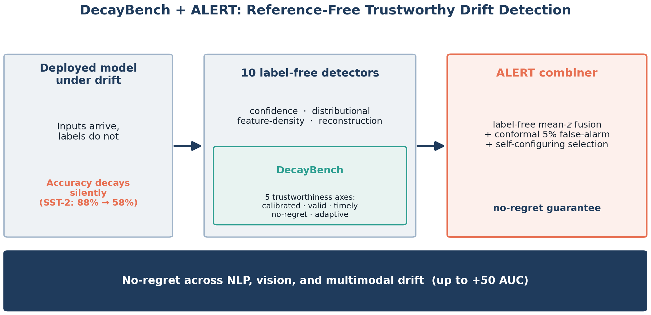
Distribution drift can substantially degrade the performance of deployed machine learning models; for example, accuracy on SST-2 can fall from 88 % to 58 % . Detecting such degradation is fundamentally challenging because deployment provides inputs but not labels, so the detection itself must be reference-free. We introduce DecayBench, the first reference-free, calibrated benchmark for evaluating drift detectors. DecayBench measures detector trustworthiness along five axes (calibrated, valid, timely, no-regret, adaptive), and compares ten existing detectors across ten NLP, vision, and multimodal datasets using paired-bootstrap significance testing. Evaluation on DecayBench shows that no existing detector is uniformly optimal. Motivated by this observation, we propose Alert, a label-free aggregation rule for drift detection. Unlike all competing combiners, it uses a label-free self-configuring selection rule with a no-regret guarantee. Alert has three contributions: (i) a dilution analysis yielding a self-configuring detector selection rule; (ii) a finite-sample conformal guarantee that controls the false-alarm probability on clean data at any prescribed level (e.g., 5 % ) for arbitrary score distributions; and (iii) a no-regret result: when no single detector dominates (constituents of comparable effect size, a condition checkable offline), Alert matches or beats the best constituent, being never significantly worse and sometimes better by a large margin; this holds across NLP, NLI, and vision (ResNet), with the largest gains under multimodal drift, and the proof identifies a dominant single detector (MMD on CLIP) as the only dilution exception. We prove the no-regret property and, across the benchmark, report its empirical counterpart, non-dominance under a paired bootstrap (Alert is never significantly worse than the best constituent), which at some operating points is statistically inconclusive rather than a strict win. Because Alert combines only embedding- and logit-based detector scores, it directly transfers across NLP, vision, and multimodal models. Empirically, Alert strictly improves over single-modality monitoring, increasing AUC by up to 25 points under mixed-modality drift and by approximately 50 points under cross-modal mismatch, where individual modality-specific detectors perform near chance. Alert also matches or outperforms the Fisher, Simes, Bonferroni, and median combiners, performs best under low-severity drift, and matches or surpasses early fusion (Concat-MMD) in both multimodal settings.

Graphical Abstract

1. Introduction

Deployed machine learning models operate in non-stationary environments: as the input stream drifts away from the training distribution, predictive accuracy can decay substantially while model confidence remains unchanged. In our benchmark (Table 7), a sentiment classifier on SST-2 [1] drops from 88 % to 58 % accuracy under graded drift, and a linguistic acceptability classifier on CoLA [2] drops from 77 % to 33 % , without any signal in the model outputs. Such failures are therefore inherently silent.
To mitigate this risk, deployed systems rely on drift detectors, which monitor an input stream and raise an alarm once the distribution has shifted sufficiently that predictions can no longer be trusted. A correct alarm enables downstream intervention such as deferral, human review, or model updating. The fundamental difficulty is that drift detection is a reference-free statistical problem [3,4]: at deployment time, inputs are observed, but labels are unavailable, so neither detector performance nor drift severity can be directly evaluated.
This creates a second-order problem: one must not only detect distribution shift without labels, but also decide which detector to trust, despite the fact that detector quality itself cannot be observed online. Existing evaluation practice does not resolve this issue [5]. Detectors are typically compared at inconsistent thresholds, against weak or task-specific baselines, without calibrated operating points or rigorous significance testing [6,7,8]. As a result, there is no principled method for selecting drift detectors under deployment constraints.
We address this reference-free detector selection problem along two axes: benchmarking and inference.
First, we introduce DecayBench, a reference-free, calibrated benchmark for drift detection. Each detector is evaluated at a fixed operating point determined using only clean data, yielding a uniform false-positive rate constraint. This calibration corresponds to a conformal threshold and induces a finite-sample, distribution-free guarantee on the false-alarm rate. The benchmark further incorporates paired-bootstrap significance testing and evaluates detectors across ten NLP, vision, and multimodal datasets using ROC-AUC, AUPRC, precision/recall at fixed false-alarm rate, and detection delay.
Beyond standard metrics, DecayBench quantifies trustworthiness along five axes: calibrated false-alarm control (the alarm fires on clean data at most a chosen target rate, e.g.,  5 % ), validity of detected drift (i.e., whether alarms correspond to real accuracy degradation), timeliness (it raises the alarm within a bounded delay after drift onset), robustness across shifts (no-regret behaviour), and adaptability to new models without labels.
Second, the benchmark reveals a structural phenomenon: after statistical control, no single detector is reliably optimal across regimes. Different detector families dominate in different settings: confidence-based methods in NLP, kernel-based tests in vision, and distance-based methods in selected shifts; none is uniformly superior across tasks, severities, or modalities.
This motivates treating drift detection as an aggregation problem rather than a single-detector selection problem: the goal is to fuse several detectors, not to crown one.
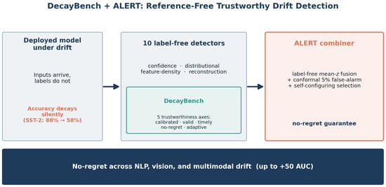
We therefore introduce Alert (Figure 1), a label-free detector aggregation rule that produces the deployment-time alarm at the end of the detection pipeline. Unlike standard combiners (e.g., Fisher [9], Simes [10], Bonferroni [11], Stouffer [12]), which weight all detectors equally and cannot drop an unhelpful one, Alert adds a label-free self-configuring step that prunes the detectors that would dilute the combination; it still aggregates the surviving detectors rather than reducing to a single one. Because its threshold is conformally calibrated, Alert inherits finite-sample false-alarm control: its false-positive rate on clean data is provably bounded at the chosen target (e.g., 5 % ) for any number of calibration batches. We further prove a conditional no-regret guarantee (Proposition A2): when the constituents have comparable effect sizes, Alert is never worse than the best constituent and can be strictly better under heterogeneous shift; when one detector’s effect size dominates, the average can be diluted below it (Corollary A2), which is exactly what the self-configuring selection targets.
Empirically, when no single detector dominates, Alert matches or exceeds every individual detector (Table 9) and every p-value combiner (Table 5). It is particularly strong under low-severity drift, where detection is most critical (Table 9). In multimodal settings, it matches or surpasses early fusion (Concat-MMD), reaching AUCs of 1.000 vs. 0.892 under compound drift (Appendix E) and 1.000 vs. 0.970 under cross-modal mismatch (Table 13). It is no-regret wherever no single detector dominates: on NLP, it is never significantly worse than the best single detector and often better at low severity (Table 9); on vision, it transfers unchanged and, on ResNet where the detectors are on par, matches or beats the best single detector, while on CLIP, where MMD dominates, MMD leads at low severity (Table 12); and in multimodal settings fusion strictly wins, significantly beating the best single-modality monitor (paired bootstrap, p < 0.001 ) even when each modality alone falls to near chance (Table 13).
Summary of contributions.
  • DecayBench: A reference-free, calibrated benchmark for drift detection with conformal false-alarm guarantees (Proposition A1), statistical significance testing (Section 4.4), and cross-modal evaluation (Table 13).
  • Alert: A label-free, self-configuring aggregation rule with finite-sample calibration (Proposition A1) and a no-regret guarantee (Proposition A2).
  • Trustworthiness measurement: A definition of reference-free drift-detection trustworthiness (Definition 3), made measurable along five axes (calibrated false-alarm control, validity, timeliness, no-regret, and adaptivity) under the label-free precondition (Section 4.4).
  • Empirical results: A significance-tested study showing that drift detectors are regime-dependent rather than uniformly optimal (Table 4), with consistent Alert gains across NLP (Table 9), vision (Table 12), and multimodal settings (Table 13), especially under low-severity (Table 9) and cross-modal drift (Table 13).
The remainder of this paper is organised as follows. Section 2 reviews related work on reference-free quality estimation, drift and out-of-distribution detection, and how such detectors are evaluated. Section 3 sets up reference-free drift detection. Section 4 introduces DecayBench: its typed and graded drift streams, its calibrated no-peeking operating point with a conformal false-alarm guarantee, its detection metrics, and its trustworthiness criterion. Section 5 presents Alert, a label-free combiner, with its dilution analysis, conformal inheritance, and self-configuring selection rule. Section 6 presents the empirical study across NLP, vision, and multimodal models: it introduces the deployed models, the datasets, and the ten benchmarked detectors, evaluates the single detectors, Alert, and competing combiners, and discusses the implications (Section 6.6). Section 7 concludes, and Section 8 covers limitations and future work.

2. Related Work

2.1. Drift and OOD Detection

A large body of literature develops detectors for distribution shift, but not their rigorous evaluation. Confidence-based methods derive anomaly scores directly from a classifier’s outputs, including maximum softmax probability [13], ODIN [14], energy [15], and later post hoc variants such as ReAct, ViM, and deep nearest neighbours [16,17,18], as well as Mahalanobis feature-density methods [19]; see Yang et al. [6] for a survey. Distributional approaches instead compare batches using kernel two-sample tests such as MMD [20], classifier two-sample tests [21], and black-box shift detection [5,22]. For NLP, DriftLens [23] compares class-conditional embedding distributions, while reconstruction-based monitors learn generative models of in-distribution data [24], despite known limitations for OOD detection [25]. Text-specific OOD work studies transformer representations [26,27,28] and confidence calibration [29,30]. Our work is complementary: rather than proposing another detector, we evaluate ten label-free detectors drawn from these families (MSP, ODIN, Energy, MMD, BBSD, Mahalanobis, KNN, DriftLens, an industrial cosine baseline, and the reconstruction monitor Recon), all computable from a forward pass of the deployed model, under one calibrated protocol (Section 4).

2.2. Evaluating Drift Detectors

Monitoring non-stationary data streams has long been studied [7,31], yet evaluation remains fragmented. OpenOOD [32] standardises primarily vision OOD detection, while WILDS [33] measures post-shift accuracy rather than label-free detection. The seminal “Failing Loudly” study [5] compares shift detectors but does not use calibrated operating points or significance testing, and conformal test martingales [34] provide sequential change detection rather than a general evaluation benchmark. Benchmarks named for “drift” address different problems entirely, including databases [8,35] and LLM agents [36]. By contrast, DecayBench is, to our knowledge, the first released benchmark for reference-free drift detection combining calibrated fixed-FPR evaluation, significance testing, detection delay, typed and graded drift streams, and multimodal coverage (Table 1).

2.3. Reference-Free Reliability Estimation and Score Combination

Drift detection is closely related to reference-free quality estimation, which predicts model reliability without labels [3,4]. Likewise, combining evidence from multiple label-free statistics has a long history, from Fisher’s and Stouffer’s methods [9,12] to recent conformal and OOD combination schemes [34,37,38]. We build directly on these ideas rather than introducing a new combination rule. Our contribution is a calibrated benchmark demonstrating that, across heterogeneous detector families, no individual detector is consistently best and a simple label-free combiner is empirically no-regret whenever no single detector dominates.

3. Problem Setup

3.1. Distribution Drift

The deployed classifier f θ acts on inputs x in an input space X , producing for each input a logit vector ( x ) R K over the K class labels and a [CLS] embedding e ( x ) R d of dimension d. Write P 0 for the in-distribution (training) input marginal, the reference against which drift is measured. At deployment, the model sees a stream of input batches B 1 , B 2 , , each a set B t = { x 1 , , x n } of n inputs drawn from a batch marginal P t .
Definition 1
(Distribution drift). A batch B t P t exhibits drift relative to P 0 when P t P 0 . We model the stream with an unknown onset t : P t = P 0 for t < t and P t P 0 for t t , possibly with graded severity. The drift is consequential when it raises the deployed classifier’s error against the true label y, E P t [ ( f θ ( x ) y ) ] > E P 0 [ ( f θ ( x ) y ) ] .
Definitions 1 and 2 formalise standard notions from the dataset-shift and reference-free out-of-distribution detection literature reviewed in Section 2 [5,6]; the trustworthiness axes of Definition 3 are, by contrast, introduced in this work. Two instances of Definition 1 bound the detectors we study. Data (input-marginal) drift changes the input distribution directly, P t ( x ) P 0 ( x ) (new vocabulary, noise, domain change); this is the silent–accuracy–loss regime and our main focus. Representation drift is a meaning-preserving map (such as paraphrase) under which the label posterior P ( y x ) is essentially unchanged, yet the induced distribution of the embedding e ( x ) shifts. Detectors differ in which of these they can see, a distinction the typology probe (Appendix C.1) makes concrete.

3.2. Drift Detection

Definition 2
(Reference-free drift detector). A drift detector is a map g from a batch to a scalar score g ( B t ) R , together with a threshold τ, that raises an alert on B t when g ( B t ) > τ . It is reference-free (label-free) when g ( B t ) depends only on the inputs { x i } and the deployed model f θ (their embeddings e i and logits i ), using no test labels, and τ is calibrated on clean ( P 0 ) data alone.
The detection problem is therefore to choose g and τ so that the alert fires under consequential drift ( t t ) but rarely on clean batches, all without deployment labels. The calibration of τ and the metrics that score g are defined in Section 4; the ten detectors we benchmark and the deployed models are introduced with the experimental setup (Section 6).

4. DecayBench: Evaluation Framework

DecayBench provides a calibrated benchmark for reference-free drift detection. It combines (i) labelled, typed, and graded drift streams; (ii) no-peeking calibration with finite-sample false-alarm guarantees; (iii) standard detection metrics, including detection delay; and (iv) a measurable notion of trustworthy drift detection.

4.1. Typed, Graded Drift Streams

We evaluate detectors on streams whose drift status is known exactly. Starting from held-out clean validation data, we generate drifted batches by applying deterministic character- and word-level perturbations at severity
ρ { 0.01 , 0.02 , 0.03 , 0.05 , 0.10 , 0.15 , 0.20 } ,
where ρ is the fraction of perturbed tokens. Clean batches receive label 0, and perturbed batches receive label 1. Low ρ produces subtle drift, while larger ρ yields progressively easier detection. Reporting performance across the full severity range avoids conclusions based only on easy drift.

4.2. No-Peeking Calibration

All detectors are evaluated at the same operating point. For each detector, we estimate a threshold τ using only held-out clean batches, never drifted or future data, by taking the ( 1 α ) quantile of the clean score distribution ( α = 5 % throughout). This fixes the deployment false-positive rate before evaluation. Throughout, calibrated is used in this conformal sense, controlling the false-alarm (false-positive) rate at the target level α , and not in the distinct sense of confidence calibration, the agreement between a model’s predicted class probabilities and its empirical accuracy; only the former is studied here.
This calibration is exactly split conformal, giving a finite-sample, distribution-free guarantee that the clean false-positive rate does not exceed α under exchangeability [34,38]. Because the guarantee depends only on score ordering, it also applies to the combined detector Alert. The proof is given in Appendix F (Proposition A1, Corollary A1).

4.3. Accuracy Metrics

For each detector, and drift severity, over a held-out set of clean (label 0) and drifted (label 1) batches with scores g ( B ) (larger means stronger evidence of drift), we report four standard detection–accuracy metrics. ROC-AUC [39] = Pr [ g ( B + ) > g ( B ) ] is the threshold-free probability that a drifted batch outscores a clean one ( 0.5 for a useless detector); AUPRC [40] summarises the precision–recall curve and is more informative under class imbalance. At the calibrated threshold τ (Section 4.2), we report precision, recall, and their harmonic mean F1 [41]. Detection delay [42] is the index of the first alerted batch as severity ramps from 0 (lower is faster; undefined if the detector never alerts). All metrics are averaged over three seeds, and reporting all four prevents a single favourable number from standing in for the whole operating curve. Algorithm 1 states the full procedure.
Algorithm 1: DecayBench protocol: calibrated drift detection and evaluation
Mathematics 14 03045 i001

4.4. Trustworthiness Metrics

Accuracy metrics rank detectors; they do not say whether a detector is trustworthy to deploy. Making “trustworthy” precise and measurable is one of this paper’s contributions: a reference-free drift detector is trustworthy to the degree that it satisfies five testable axes, each answering a concrete deployment question. Prior evaluations test at most one or two of these in isolation; DecayBench makes all five measurable at once.
Definition 3
(Trustworthiness metrics). A drift detector operates label-free, using no test labels at deployment; this is the precondition that defines the reference-free setting. Within it, the detector (and its deployment-time alert) is trustworthy to the degree that it is (i) calibrated, holding the false-alarm rate on clean data at a controlled target; (ii) valid, in that the drift it flags is consequential, associated with real accuracy loss; (iii) timely, alerting within a bounded delay of drift onset; (iv) no-regret, never significantly worse than the individual signals it is built from (proved as Proposition A2; reported empirically as non-dominance under a paired bootstrap); and (v) adaptive, configurable from clean data so it degrades gracefully across tasks and backbones.
Notation. A detector g maps a batch B to a scalar score g ( B ) R (larger means stronger evidence of drift) and alerts when g ( B ) exceeds the calibrated threshold τ of Section 4.2; write A g ( B ) = [ g ( B ) > τ ] { 0 , 1 } for that alert, with  [ · ] the indicator. Clean batches are drawn B P 0 and drifted batches B P ρ at severity ρ > 0 ; Pr B P 0 is the probability over a clean batch and E P 0 , E P ρ are expectations under the clean and drifted batch distributions. Let a ( B ) [ 0 , 1 ] be the deployed classifier’s accuracy on B, AUC ( g ) [ 0 , 1 ] its detection ROC-AUC, and  α ( 0 , 1 ) the target false-positive rate. Each axis is then a testable property, answering a deployment question and established by a specific measurement.
  • Calibrated. Can an operator trust and budget the alarm? The clean false-alarm rate is held at the target,
    Pr B P 0 A g ( B ) = 1 α ( α = 0.05 ) ,
    fixing τ on clean data alone (Section 4.2); we ground this in a finite-sample conformal guarantee (Proposition A1) that the combiner inherits (Corollary A1). Calibration plays a dual role, both an axis and the common operating point at which the others are read.
  • Valid. Does an alert mean something has actually gone wrong? The flagged drift is consequential: deployed accuracy is strictly decreasing in severity,
    E P ρ [ a ] < E P 0 [ a ] for   every   ρ > 0 ,
    verified by the accuracy–decay study (Section 6.4.2).
  • Timely. Does the alert arrive in time to act? Given a severity ramp ( B t ) t 1 (a stream of batches with drift onset at t = 1 ) and a delay budget D max , the detection delay is bounded,
    D ( g ) = E min { t 1 : A g ( B t ) = 1 } D max ,
    measured in Section 6.4.3.
  • No-regret. Is the deployed monitor a dependable default? For M constituent detectors g 1 , , g M , their combiner g = A l e r t , and a tolerance ε 0 , the regret R (the AUC gap to the best constituent) is non-positive up to significance,
    R = max 1 k M AUC ( g k ) AUC ( g ) ε ,
    with a paired bootstrap failing to reject AUC ( g ) AUC ( g k ) for every k (Table 9; empirically ε 0 ).
  • Adaptive. Will it still work on the next task or backbone? A label-free selector S maps a deployment j’s clean data C j to a detector subset g S ( C j ) ; writing AUC j for detection ROC-AUC on deployment j, re-selecting is never worse than transferring a family chosen on a different deployment j ,
    AUC j g S ( C j ) AUC j g S ( C j ) ( j j ) ,
    realised by the label-free contextual selection (Section 5.3).
The axes are not new in isolation: they synthesise established notions, calibrated coverage from conformal prediction [34,38], no-regret from online learning [43], and bounded detection delay from change-point detection [42]. The contribution is to make all five simultaneously measurable and label-free for drift detection.

5. Alert: A Calibrated Label-Free Combiner

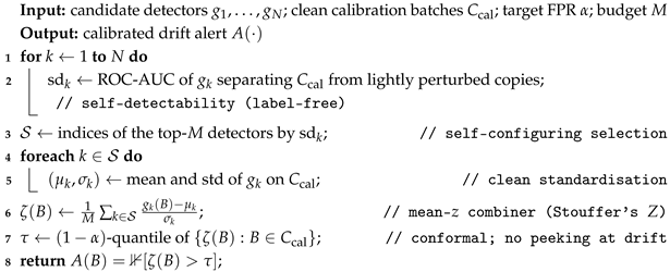
Alert is our deployment-time method. It does not introduce a new drift signal; instead, it combines existing detectors into a single calibrated drift alert. The combination rule itself is classical. Our contributions are threefold: (i) showing that the combined detector inherits the finite-sample calibration guarantee of Section 4.2; (ii) establishing conditions under which the combiner is no-regret; and (iii) introducing a label-free rule that automatically selects which detectors to combine. Formal results are given in Appendix F.

5.1. Combining Complementary Detectors

Different detectors capture different manifestations of drift. MMD measures changes in embedding distributions; energy and ODIN measure predictive confidence; Recon measures reconstruction error; and DriftLens measures changes in class-conditional embedding geometry.
Alert first standardises every detector using only the clean calibration batches: writing s k = g k ( B ) for the k-th detector’s score on batch B,
z k = s k μ k σ k ,
where ( μ k , σ k ) are the mean and standard deviation of s k on clean data. The standardised scores (or their equivalent clean-calibrated p-values) are then combined into a single statistic; Alert’s default is their mean (equivalently Stouffer’s Z), and we compare it against the median, Fisher, Simes, and Bonferroni rules in Section 6.4.4. This follows the classical multiple-testing framework of Fisher [9] and Stouffer [12], applied here across heterogeneous detector families.

5.2. Why Combining Helps

When the constituent detectors carry complementary information, averaging their standardised scores reinforces the shared drift signal while reducing independent noise, improving detection over any single detector. When the constituents have comparable effect sizes, this yields a no-regret combiner; on the NLP benchmark, Alert is never significantly worse than its best constituent, and is significantly better where their signals are complementary (Table 9). When one detector’s effect size instead dominates, the average can fall below it (Corollary A2). Empirically, no-regret holds wherever no single detector dominates: NLP (Table 9), NLI and vision (Table 12), and multimodal drift, where the gain is largest; CLIP single-modality drift, where MMD dominates, is the predicted dilution exception. Because the alert threshold is calibrated exactly as in Section 4.2, the combined detector inherits the same finite-sample false-positive-rate guarantee.
The principal failure mode is dilution: including detectors with little or no drift signal can weaken the combined statistic. Appendix F (Propositions A2 and A3, Corollary A2) formalises these results under a location-shift model, deriving the M signal amplification, its extension to correlated detectors, and the precise condition under which dilution occurs. Section 6.4.4 confirms these predictions empirically.

5.3. Label-Free Detector Selection

The theoretical analysis suggests that combining every available detector is unnecessary and can even be harmful. We therefore make Alert self-configuring by selecting detectors using only clean calibration data.
For each detector, we estimate its self-detectability: the ROC-AUC separating clean calibration batches from lightly perturbed copies generated by the benchmark itself. This procedure requires no deployment labels and never accesses the evaluation stream.
We then combine only the top-M detectors by self-detectability (we report M { 3 , 5 } ). Intuitively, self-detectability estimates a detector’s effect size under small perturbations, so retaining high-scoring detectors while removing near-zero ones maximises the combiner’s signal-to-noise deflection and avoids the dilution characterised in Appendix F (Proposition A3, Corollary A2). Section 6.4.5 evaluates this selection rule. Algorithm 2 states the full procedure: label-free selection, clean standardisation, mean-z combination, and the conformal threshold it inherits from Section 4.2.    
Algorithm 2: Alert: label-free self-configuring drift alert
Mathematics 14 03045 i002

6. Experiments

We evaluate the paper’s two contributions: DecayBench, a calibrated benchmark for reference-free drift detection, and Alert, a label-free combiner of existing detectors. Unless otherwise stated, we evaluate ten label-free detectors on SST-2 and CoLA under seven drift severities and three random seeds, using the full validation split in batches of size 64; thresholds are calibrated to a 5 % false-positive rate on held-out clean batches only. We further test transfer to natural domain shift, a three-class NLI task (MNLI), and vision and multimodal backbones.

6.1. Datasets and Deployed Models

The primary deployed models are the GLUE [44] tasks SST-2 [1] and CoLA [2], each with a fine-tuned bert-base-uncased classifier [45] monitored by the detectors; the training split defines the in-distribution reference, and the validation split provides the clean stream from which drifted streams are constructed. DecayBench additionally covers natural domain shift (IMDB [46], Yelp [47], and Amazon [48] sentiment), a three-class sentence-pair task (MNLI [49]), and modality transfer to vision (CIFAR-10-C [50,51], STL-10 [52]) and multimodal (CLIP [53] image-caption) backbones, ten datasets in all (Table 2), introduced where they are used in the experiments that follow.

6.2. Baseline Detectors

We evaluate ten existing label-free detectors spanning five families (Table 3); each maps a batch B t to a scalar drift score using only the deployed classifier f θ and its [CLS] embeddings e i R 768 (the bert-base-uncased hidden size) or logits i R K (over the K classes), and only Recon [24] is trained (an auxiliary autoencoder). All are established prior work; we claim none as our own. Our contributions are the benchmark (Section 4) and Alert, a label-free combiner that aggregates these signals into one deployment-time alert (Section 5.1). Full score definitions, the Recon autoencoder and its drift-score algorithm, and Recon’s three-signal typology decomposition are in Appendix B; no signal is privileged, and all are scored identically under the protocol of Section 4.

6.3. Label-Free Detector Performance

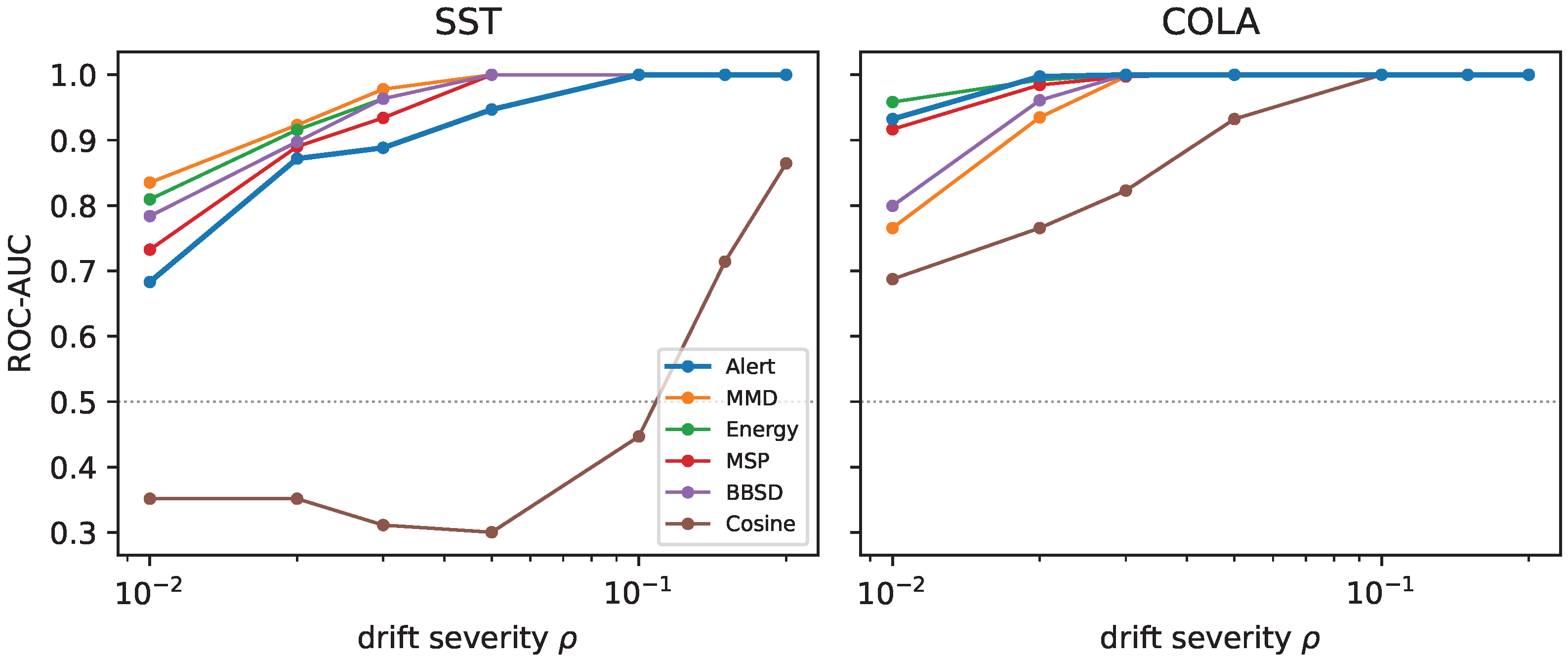
Table 4 reports detection ROC-AUC across tasks and severities and exposes the benchmark’s central finding: no single detector wins. Training-free MMD and energy are the strongest overall and consistently match or beat the trained reconstruction monitor, while the industrial cosine baseline collapses to near-random; yet, which method leads still flips with task and severity. The full severity curves (Figure A2), the calibrated-operating-point metrics (Table 6), and three further signals (DriftLens, ODIN, KNN) all tell the same story. This instability, not any fixed winner, is what motivates a combiner.
Table 5 illustrates why Alert works: on SST-2, its mean-z rule matches or beats every classical combiner (Fisher, Simes, Bonferroni, GLRT, median), so the advantage comes from calibration and correlation structure, not a bespoke aggregation. The location-shift model of Proposition A2 predicts the observed gains, with the correlation-corrected form closest to the measured AUC (Table A7); fusion gain is thus governed by redundancy among detectors, not their count.

6.4. Trustworthiness

Beyond detection accuracy, we evaluate every detector and Alert on the five trustworthiness axes of Definition 3, in their defining order: calibrated false-alarm control, validity, timeliness, no-regret, and adaptivity.

6.4.1. Calibrated

Table 6 shows the leading detectors and Alert stay accurate at the calibrated operating point: at the common 5 % false-positive target fixed on clean data alone, training-free MMD and energy reach precision and recall at or near 1.0 on both tasks, and Alert attains perfect precision and recall at a measured 0.0 false-positive rate, so the no-peeking calibration that gives every detector one controlled threshold (the conformal guarantee of Proposition A1) costs nothing in detection quality.

6.4.2. Valid

Table 7 shows the injected drift is consequential: deployed accuracy falls monotonically with severity, from  0.88 to 0.58 on SST-2 and from 0.77 to 0.33 on CoLA, with comparable decay under natural domain shift (IMDB, Yelp). A benchmark is informative only when its perturbations cause genuine degradation, so every detection score below reflects real accuracy loss rather than cosmetic noise. True labels are used for this check alone, never by any detector.

6.4.3. Timely

Table 8 shows that the strongest detectors also alert earliest, and Alert stays in the fastest tier on both tasks, so its accuracy gains cost nothing in timeliness.

6.4.4. No-Regret

Table 9 demonstrates the main result: on this on-par detector pool, Alert turns the unstable signals into one calibrated score that is never beaten. It attains the highest ROC-AUC at every SST-2 severity (panel a) and matches the best single detector on CoLA, where a confidence score already saturates. Paired-bootstrap tests (panel b) confirm Alert is never significantly worse than any constituent at the hardest severity ρ = 0.01 , the no-regret guarantee of Proposition A2. Where the paired-bootstrap p-value is large (e.g., p = 0.579 for MMD and p = 0.393 for Energy in panel b), the comparison is statistically inconclusive in either direction; we read these cells as non-dominance (Alert is not significantly worse), not as strict wins. Alert is therefore a simple, label-free default that deploys without knowing in advance which detector would have won.

6.4.5. Adaptive

Table 10 shows Alert also configures itself. Choosing detector families by self-detectability on clean data alone recovers the right family per task with no labels or tuning (panel a), and helps most under mismatch: when a fixed family meets the wrong task or a RoBERTa [55] backbone, re-selection recovers up to + 0.136 ROC-AUC (panel b).

6.5. Generalisation

Alert and the benchmark protocol generalise well beyond the SST-2/CoLA token-noise setting. We test three forms of transfer in turn: natural domain shift, single-modality backbones, and multimodal fusion. Table 11 begins with natural domain shift: monitoring clean SST-2 against whole out-of-domain corpora (IMDB, Yelp, which drop classifier accuracy to ∼ 0.78 ), confidence scores, MMD, and Alert all detect the shift at ROC-AUC 1.000 , while the industrial cosine baseline collapses to near-zero ( 0.000 and 0.044 ) despite the real accuracy loss.
Table 12 extends the protocol to new single-modality backbones: a three-class NLI task (MNLI, panel a) and vision models (ResNet-18 [56] and zero-shot CLIP, panel b). Strong detectors stay strong, and the cosine baseline still fails. The outcome follows detector dominance, as the theory predicts: on MNLI and ResNet, where no single detector dominates (on ResNet all detectors fall within 0.85 0.91 ), Alert matches or beats the best single detector ( A l e r t = 0.920 vs. best single 0.913 at the lowest ResNet severity, never significantly worse); on CLIP, where MMD dominates ( 0.986 vs. 0.933 for the next detector), Alert stays competitive but MMD leads at low severity, exactly the dilution regime of Corollary A2.
Table 13 closes with multimodal drift, the one setting where fusion strictly wins: under mixed-modality and cross-modal mismatch drift invisible to any single stream, Alert reaches ROC-AUC 1.000 , while single-modality monitors sit near chance. It improves on the best single-modality monitor by up to 25 points (mixed) and roughly 50 points (mismatch), significant under a paired bootstrap ( p < 0.001 ), and matches or surpasses early fusion (concat-MMD [20], 0.970 on mismatch). The cross-modal alignment score is essential: a marginals-only Alert catches modality corruption but is near chance on mismatch ( 0.542 ), and adding alignment to the fused family recovers 1.000 . These results confirm the benchmark’s conclusions are not specific to one dataset or modality. Real-pair, dead-channel, and larger-backbone variants confirm this (Appendix E).

Is the Multimodal Gain the Combiner or the Alignment Feature?

On caption mismatch, the alignment score alone already reaches ROC-AUC 1.000 , so we isolate the source of Alert’s performance (Table 14). Given the same family that includes the alignment member, every combiner, our mean-z, a naive unstandardised mean, and a supervised logistic regression, reaches 1.000 , whereas a fusion without the alignment member (marginals only) stays near chance ( 0.417 ). The gain on this task is therefore attributable to including the cross-modal alignment member, which Alert selects label-free, not to the specific aggregation rule; this is exactly the dilution regime of Corollary A2, where one dominant member makes the combiner reduce to it. The aggregation rule earns its keep in the settings where no single member dominates, the mixed-modality columns of Table 13 and the on-par detector pools of Table 9 and Table 12.

6.6. Discussion

The central finding is not that some detectors beat others, but that detector performance is governed by drift geometry: apparent superiority is often an artefact of the chosen baseline or perturbation, and against strong training-free baselines such as energy and MMD, learned reconstruction monitors are no longer dominant. Detector families respond to different statistical signals, so their assumptions break in different and sometimes opposite ways; for example, token-level corruption can pull representations toward the training centroid and invert Mahalanobis-style scores while the same statistic stays effective under natural shift, which is why rankings vary across tasks and severities. Drift detection is therefore not a model-selection problem with one optimal solution but a context-dependent one, and robustness comes primarily from calibration and combination rather than detector complexity: calibrated confidence scores are strong defaults, distributional tests help when embeddings and covariate shift are expected, and fusing complementary detectors is more reliable than betting on a single best one. Progress should thus be measured less by new detector design and more by understanding when and why detectors fail.

7. Conclusions

We introduced DecayBench, a calibrated benchmark for reference-free drift detection that enforces consistent evaluation under controlled drift severity, calibrated thresholds (a clean false-positive target that admits a finite-sample, distribution-free conformal interpretation), and standardised metrics. Across ten representative label-free detectors, we find that no method is uniformly dominant. We further propose Alert, a label-free combiner that aggregates detector signals into a single calibrated alert. Whenever no single detector dominates, it is no-regret, matching or beating the best constituent across NLP, NLI, and vision and beating it by a large margin under multimodal drift, never significantly worse; a dominant single detector (the dilution corollary, e.g., MMD on CLIP) is the only exception. This condition is checkable offline, and the guarantee follows from the comparable-effect-size regime of our analysis. Together, these contributions establish a reproducible evaluation setting and a simple but effective aggregation mechanism that reveal how much robust signal already exists in standard detectors when they are measured consistently and combined carefully. The result is a clearer path forward for reliable drift detection grounded in calibration, comparability, and compositionality of existing signals.

8. Limitations and Future Work

We study reference-free drift detection, deciding from unlabelled data when to raise an alert, on encoder-based classification models under synthetic and natural shift. We do not address concept drift, where the label changes with no observable input change and which unlabelled inputs cannot reveal. Alert is also only as strong as the detectors it fuses: its no-regret guarantee assumes an appropriate detector family, and its label-free selection assumes the self-perturbation probe resembles the real drift. When that fails, as under a cross-modal mismatch no single-modality probe can mimic, selection can drop the decisive detector and a single strong detector may win.
What to do after an alert (human review, abstention, adaptation, or retraining) is outside our scope, as are multilingual and long-horizon deployment, richer distribution shift, and foundation-model backbones. Because DecayBench fixes one calibrated protocol and metric set, any new detector or deployment setting can be scored the same way and compared head-to-head with the baselines reported here.   

Supplementary Materials

The following supporting information can be downloaded at: https://www.mdpi.com/article/10.3390/math14173045/s1, S1: DecayBench reproducibility package, comprising the frozen, ground-truth-labelled evaluation set and its manifest; the calibrated evaluation harness with its detector API (build_benchmark.py, eval_benchmark.py); the deployed classifiers and reconstruction monitors; the experiment scripts for the NLP, vision (ResNet), CLIP/multimodal, MNLI, and RoBERTa studies; and the raw result files (JSON) underlying every reported table and figure.

Author Contributions

J.X. made a significant intellectual contribution to the theoretical development, system or experimental design, prototype development, and/or the analysis and interpretation of data associated with the work contained in the article. She also drafted, revised, and approved the article. Y.T. made a significant intellectual contribution to the theoretical development associated with the work contained in the article. She also revised and approved the article. All authors have read and agreed to the published version of the manuscript.

Funding

This research was supported in part by eBay Inc. and the U.S. National Science Foundation (NSF) under Award No. 2425802.

Data Availability Statement

DecayBench, the frozen, labelled eval set, the evaluation harness with its detector API, and the deployed models, are provided as Supplementary Materials with this submission and will be publicly released. The eval set is fully regenerable from public data (GLUE: SST-2, CoLA; IMDB; Yelp) by the build_benchmark.py script; the reference results, the Alert combiner, and the significance, delay, and scope-expansion (MNLI) experiments are reproduced by the released scripts (Appendix G).

Acknowledgments

The authors used AI to assist with experiment and analysis code, statistical analysis, literature search, and polishing of this manuscript. All results and claims were verified by the human authors, who take full responsibility for the content.

Conflicts of Interest

Author Jia Xu was employed by the company 8AI LLC. The remaining authors declare that the research was conducted in the absence of any commercial or financial relationships that could be construed as a potential conflict of interest.

Appendix A. Appendix Map (Guide to Supplementary Materials)

This appendix is organised to make the evaluation protocol and claims of the main paper fully traceable. We summarise the role of each section below so that readers can quickly locate definitions, robustness checks, and reproducibility details.
  • What is defined (detectors and scoring functions). Appendix B formally defines all ten detector families used in the main experiments, including (i) training-free baselines (cosine, MMD, Mahalanobis, energy, MSP, ODIN, KNN, DriftLens, BBSD), and (ii) the trained reconstruction-based monitor (Recon). These definitions specify exactly what is compared in Table 3.
  • What the detectors actually measure (behavioural validity). Appendix C analyzes failure modes and identifiability: structured reconstruction signals do not reliably infer drift type (Table A1), and performance is strongly batch-size dependent (Table A2). These results explain why aggregate ROC-AUC alone is insufficient to characterise detector quality.
  • What happens under realistic drift regimes (robustness). Appendix D evaluates detectors under (i) graded natural-drift mixtures (Table A3) and (ii) temporal real-world drift (Amazon reviews). The key finding is that synthetic severity rankings generalise to real drift, while some real temporal shifts are benign (no accuracy decay, no meaningful alarms).
  • What happens beyond the single-modality setting (extensions). Appendix E reports the supporting tables relocated from the main text, together with multimodal and compound-drift experiments: real image-caption pairs, cross-modal mismatch, and multi-channel monitoring with a deliberately useless signal. The results show that cross-modal alignment and robust aggregation dominate in heterogeneous settings.
  • Operating-point validity (precision/recall and calibration). Appendix E also reports precision/recall at a fixed false-positive rate and AUPRC, confirming that ROC-AUC trends are not artefacts of thresholding and that training-free detectors remain competitive at calibrated operating points.
  • Why the method works (theory). Appendix F provides two guarantees: (i) a conformal, distribution-free false-positive control result for calibrated thresholds, and (ii) a no-regret analysis showing that averaging standardised detector scores improves signal-to-noise under a location-shift model, explaining the empirical success of Alert.
  • How to reproduce everything (benchmark release). Appendix G describes DecayBench, including frozen evaluation sets, calibration protocol, detector API, and full script list. All results are reproducible from public data with fixed seeds and deterministic batching.
  • Notation and equations. Appendix H and Appendix I provide a complete reference for symbols and scoring functions used throughout the paper.
  • How to read this appendix. If the reader is interested in:
The appendix is structured so that every major claim in the main paper can be traced to a definition, experiment, and robustness check.

Appendix B. Detector Definitions

This appendix gives the score definitions for the ten detectors of Table 3. Each maps a batch B t to a scalar drift score using only the deployed classifier f θ and its [CLS] embeddings e i R 768 (last hidden state) or logits i R K ; all are established prior work, and only Recon is trained.

Appendix B.1. Trained Reconstruction Monitor (Recon)

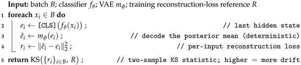
Recon [24] is a variational autoencoder m ϕ on the classifier’s [CLS] embeddings, with encoder q ϕ ( h z ) , decoder p ϕ ( e ^ h ) , and a 16-dimensional latent h. It is trained on in-distribution embeddings to minimise reconstruction error plus a latent-normality term. At deployment, we score each input by its reconstruction loss  r i = e ^ i e i 2 2 , computed deterministically with the posterior mean (no sampling). The batch drift score is the Kolmogorov–Smirnov distance between the batch’s reconstruction-loss distribution and a fixed training reference R:
g R e c o n ( B t ) = KS { r i } i B t , R ,
where KS is the two-sample Kolmogorov–Smirnov statistic. Higher means more drift. A distributional (KS) score is more sensitive than a single mean reconstruction error, which we found does not separate drift at all (Algorithm A1).
Algorithm A1: Recon batch drift score
Mathematics 14 03045 i0a1

Appendix B.2. Training-Free Baselines

For a batch B = { x i } with embeddings e i , softmax p i = softmax ( i ) , training centroid e ¯ , training reference sample E ref , and training Gaussian N ( μ , Σ ) :
g C O S ( B ) = 1 n i e i e ¯ e i e ¯ ( lower   =   drift ;   S A G E M A K E R - style )
g MMD ( B ) = 1 n i φ ( e i ) 1 | E ref | z E ref φ ( z ) H 2 ( RBF   kernel ,   median   bandwidth )
g M A H A L A N O B I S ( B ) = 1 n i ( e i μ ) Σ 1 ( e i μ ) ( Σ 1   by   Ledoit - Wolf   shrinkage )
g BBSD ( B ) = 1 K k KS { p i , k } i , P k ref ( KS   on   softmax ,   per   class )
g E N E R G Y ( B ) = 1 n i log k exp ( i , k ) ( higher   energy   =   more   OOD )
g MSP ( B ) = 1 1 n i max k p i , k ( lower   confidence   =   drift )
g ODIN ( B ) = 1 1 n i max k softmax ( i / T ) k ( temperature   T ;   lower   =   drift )
g KNN ( B ) = 1 n i d ( k ) e i , E ref ( k - th   nearest   training   embedding )
g D R I F T L E N S ( B ) = 1 K c FD N c B , N c ref ( per - class   Fréchet   dist . ;   PCA - 64 )
ODIN implementation. We use ODIN in its temperature-scaled-confidence form. The batch score is Equation (A8), g ODIN ( B ) = 1 1 n i max k softmax ( i / T ) k , with temperature T = 1000 (the default of Liang et al. [14]), aggregated as the batch mean; higher values indicate drift. We omit the input-perturbation step of the original method: it is a per-example gradient ascent on the confidence designed for single-sample OOD scoring, and it is incompatible with our forward-pass-only, batch-level, reference-free protocol (no backpropagation through the deployed model), while also changing the cost model shared by all ten detectors. We therefore report the temperature-only variant and note it as a simplification of ODIN. No detector hyperparameter is tuned on drifted or labelled data: T = 1000 is fixed a priori, as for every other detector.
The cosine baseline is the deployed industrial check (SageMaker-style) the original monitor was compared against, not a strawman we introduce: a benchmark earns its keep precisely by exposing when a fielded detector fails. When a detector’s ROC-AUC falls below 0.5 , as cosine does throughout and as the CLIP zero-shot energy of Section 6.5 does on images, its score is anti-correlated with drift. This is itself a useful, actionable signal, namely that the score’s orientation must be flipped or recalibrated before deployment, not random noise; our protocol surfaces it instead of hiding it behind a single favourable summary number. We nonetheless keep such detectors at their raw orientation in every table so that the failure is visible rather than silently corrected. MMD [20] and BBSD [5] are distributional two-sample tests; Mahalanobis [19] is a feature-space density score; and Energy [15] and MSP [13] are confidence scores available from any classifier at no extra cost. ODIN [14] is temperature-scaled confidence (temperature T); KNN [18] is the distance to the k-th nearest training embedding d ( k ) ; and DriftLens [23] averages the Fréchet distance FD between the per-predicted-class batch and reference embedding Gaussians N c B , N c ref in a PCA-64 space. Empirical results for these three are in Appendix E.3.

Appendix B.3. Drift-Type Typology Decomposition

The Recon model exposes three structured signals, the reconstruction score s D of Equation (A1), a confidence signal s C = 1 max k softmax ( ) ¯ , and a latent signal s L (Mahalanobis distance in embedding space). A natural hope is that these jointly identify the type of drift (input-marginal versus representation-level), which a single score cannot. We test this directly in Appendix C.1 by training a typology classifier on [ s D , s C , s L ] and comparing it to single-signal and energy-only classifiers.

Appendix C. Behavioural Analysis of Detectors

Beyond aggregate ROC-AUC, we examine what the detectors actually measure and where they fail.

Appendix C.1. Typology: Structured Signals Do Not Reliably Diagnose Drift Type

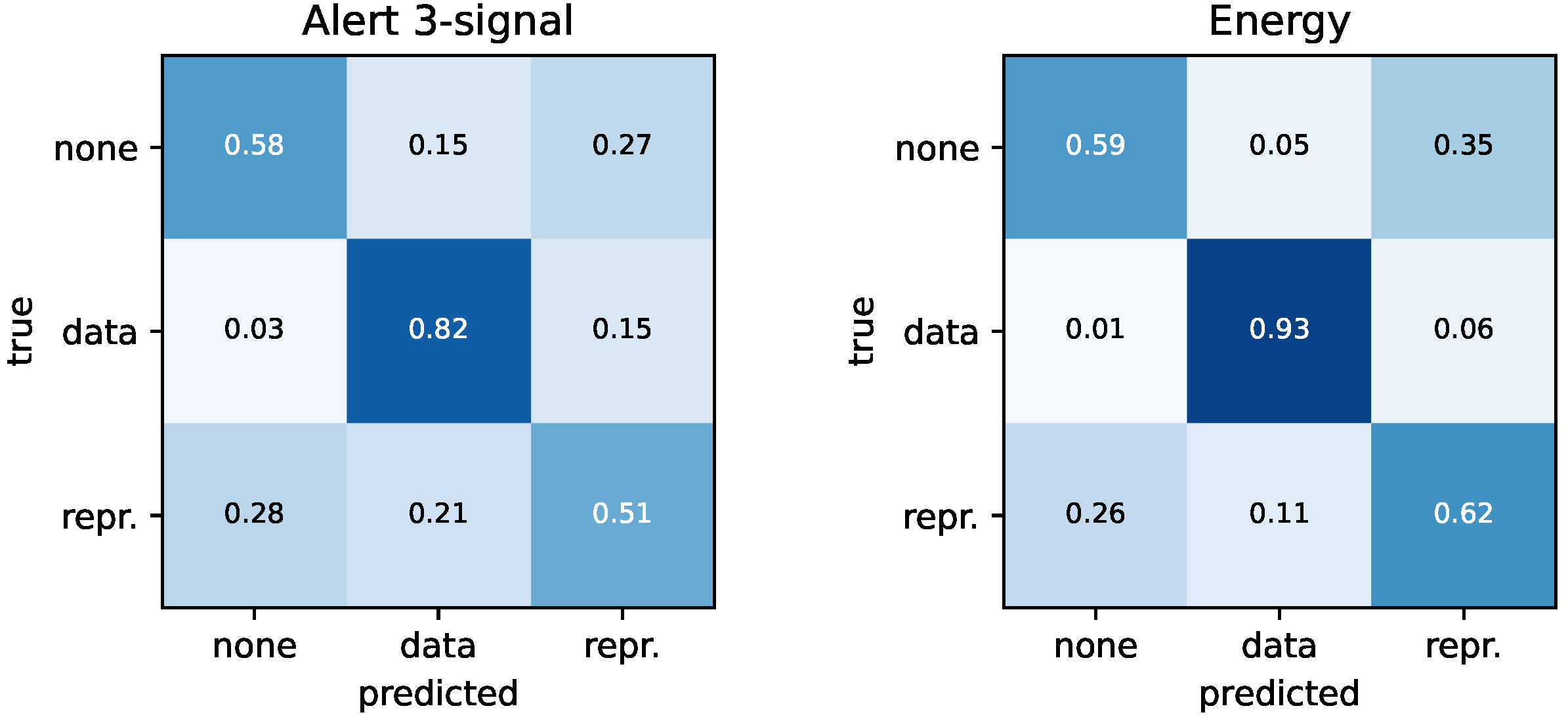
Table A1 tests whether Recon’s three signals classify drift type (none / data / representation) better than a single score. They do not reliably: a single energy score is the best typology head on average and on SST-2; the structured signals win only on CoLA. Representation-level (paraphrase) drift is the hardest case, often confused with clean data (Figure A1). The structured-signal hypothesis is therefore not supported in general.
Table A1. Structured signals do not reliably diagnose drift type. Drift-type classification macro-F1 (three classes: none/data/representation; mean over seeds). A logistic head is trained on Recon’s three signals [ s D , s C , s L ] jointly, on each signal alone, and on a single energy score; bold marks the best head per task. Energy is best on average, and on SST-2, the structured signals help only on CoLA. Representation (paraphrase) drift is the hardest, often confused with clean data.
Task [ s D , s C , s L ] s D Only s C Only s L OnlyEnergy Only
SST-2 0.380 0.459 0.454 0.303 0.586
CoLA 0.881 0.680 0.600 0.881 0.805
Mean 0.631 0.570 0.527 0.592 0.696
Figure A1. Structured signals confuse representation (paraphrase) drift with clean data, no better than energy alone. Row-normalised drift-type confusion (summed over tasks and seeds) for the Recon three-signal head (left) and a single energy score (right).
Mathematics 14 03045 g0a1

Appendix C.2. Sensitivity to Batch Size

Distributional detectors depend on how many inputs each decision aggregates. Table A2 varies the batch size on SST-2. Recon’s KS-based score needs large batches: at batch sizes 16 to 32 it is near chance for subtle drift (≤ 0.63 at ρ = 0.02 ), rising to near-perfect only at batch sizes 64 to 128. Small-batch monitoring is therefore a real limitation; the distributional test has too little to work with per decision.
Table A2. Recon needs large batches: detection degrades sharply as batches shrink. Recon ROC-AUC versus batch size (SST-2, seed 42); the KS test needs enough samples per decision.
Batch Size ρ = 0.01 0.02 0.03 0.05 0.10
16 0.528 0.615 0.626 0.703 0.808
32 0.530 0.635 0.605 0.606 0.864
64 0.758 0.802 0.940 1.000 1.000
128 0.500 1.000 0.944 1.000 1.000

Appendix D. Robustness to Drift Regimes

We test whether the synthetic-drift conclusions hold under real, graded, and temporal drift.

Appendix D.1. Graded and Temporal Natural Drift

A whole-corpus shift is, however, easy: every reasonable detector saturates, so Table 11 confirms cosine fails but cannot rank the rest. To discriminate detectors on natural drift, we therefore grade it, building a real severity ramp that mixes clean SST-2 with a fraction ρ nat { 0.05 , , 0.5 } of genuine out-of-domain sentiment (no synthetic perturbation). Table A3 reports the IMDB ramp. Now the curve is informative and tells the same story as the synthetic protocol: at 5 % natural contamination the task is hard for everyone (ROC-AUC 0.5 0.65 ) and rises smoothly to ≈ 0.99 at 50 % ; the free confidence scores (energy, MSP, ODIN) and DriftLens lead, the trained Recon monitor lags, and cosine sits below chance throughout. Alert is again no-regret and is the best detector at moderate natural drift ( 0.918 at ρ nat = 0.2 ); the Yelp ramp is similar (Alert best at ρ nat = 0.3 0.5 ). The benchmark’s ranking is thus not an artefact of synthetic noise; it reproduces on graded real drift. Quantitatively, the detector ROC-AUC ordering under synthetic and natural drift agrees (Spearman ρ = 0.68 between the synthetic ρ = 0.05 ranking and the IMDB ρ nat = 0.2 ranking on SST-2), so the synthetic protocol predicts the natural-drift ranking it is meant to stand in for.
Table A3. A graded natural-drift ramp discriminates detectors that a whole-corpus shift cannot. Graded natural-drift detection ROC-AUC (SST-2 mixed with a fraction ρ nat of IMDB sentiment; mean over three mixing seeds; no synthetic perturbation), unlike the whole-corpus shift in Table 11. Bold = best per column.
Detector 0.05 0.10 0.20 0.30 0.50
Energy 0.639 0.653 0.816 0.809 0.980
MSP 0.646 0.565 0.789 0.816 0.959
ODIN 0.599 0.653 0.837 0.891 0.980
DriftLens 0.612 0.680 0.844 0.837 0.993
MMD 0.585 0.673 0.830 0.891 0.980
Recon 0.497 0.541 0.745 0.544 0.789
SageMaker (cosine) 0.320 0.381 0.197 0.272 0.075
Alert (ours) 0.592 0.748 0.918 0.891 0.993

Temporal Drift in the Wild, and the Benign-Drift Check

The drift above is induced. To probe genuinely uncontrolled drift, we also apply the sentiment classifier to Amazon product reviews [48] binned by year, taking 2016 as the reference and 2018, 2020, and 2022 as candidate drift. The honest finding is that this temporal drift is benign: classifier accuracy is essentially flat and non-monotonic across the six years ( 0.76 in 2016 versus 0.77 , 0.72 , 0.73 in 2018/2020/2022, a swing under five points with no decay). Correspondingly, no reference-free detector raises a consistent alarm: the free scores hover near chance and disagree across years (e.g., energy ROC-AUC 0.29 0.71 , MMD  0.30 0.77 ), and the Alert combiner stays near 0.5 . This is the right behaviour, not a failure: it is the contrapositive of the validity study (Section 6.4.2). Where drift does not cost accuracy, a trustworthy detector should not manufacture a consequential-drift signal, and the clean-calibrated protocol does not over-fire on benign year-to-year change.

Appendix E. Additional Experimental Results

Supporting tables relocated from the main text, together with the multimodal, compound-drift, and operating-point results.

Appendix E.1. Detection Severity Curves

Full ROC-AUC severity curves for the detectors in Table 4.
Figure A2. Graded, non-saturated severity curves keep the detector ranking informative. Detection ROC-AUC versus drift severity (per task; mean over three seeds, log-scaled ρ ).
Mathematics 14 03045 g0a2

Appendix E.2. Supervised Upper Bound

Table A4 shows that a supervised detector given labelled drift can win at the hardest severities, but only by assuming the deployment drift is known in advance, which the reference-free setting forbids; Alert uses no such labels.
Table A4. A supervised detector can beat the free scores given drift labels (ROC-AUC; trained on ρ { 0.05 , 0.10 , 0.20 } , tested on held-out low severities). The probe and deep-kernel MMD [57] need labelled drift; Alert uses none. Bold = best per column.
DetectorSST-2CoLA
ρ = 0.01 0.02 ρ = 0.01 0.02
Supervised probe (trained) 0.978 1.000 0.734 0.977
Deep-kernel MMD (trained) 0.967 1.000 0.844 1.000
Energy (free) 0.791 0.923 0.953 0.984
MMD (free) 0.813 0.912 0.758 0.930
Alert (free, ours) 0.879 0.934 0.875 0.969

Appendix E.3. Additional Signals: DriftLens, ODIN, KNN

Beyond the seven detectors evaluated so far, we benchmark three further label-free signals defined in Appendix B: DriftLens [23] (per-predicted-class Fréchet distance), ODIN [14] (temperature-scaled confidence), and a deep KNN distance to the training embeddings [18]. Table A5 reports ROC-AUC. DriftLens is the strongest single signal on SST-2 at the hardest severity ( 0.846 at ρ = 0.01 , above MMD), and ODIN is strong on both tasks; but neither is uniformly best (DriftLens is weak on CoLA, 0.638 ), and KNN collapses on CoLA ( 0.031 ) exactly as Mahalanobis does, confirming that distance-to-training-data geometry is unreliable under token noise.
Table A5. The three extra detectors are not uniformly best either. Additional label-free signals (ROC-AUC, mean over three seeds): DriftLens leads on SST-2 at low severity, KNN fails on CoLA like Mahalanobis. Bold indicates the best result per column.
SignalSST-2CoLA
ρ = 0.01 0.03 0.05 0.01 0.03 0.05
DriftLens 0.846 0.982 1.000 0.638 0.867 0.917
ODIN 0.817 0.967 1.000 0.919 0.997 1.000
KNN 0.623 0.582 0.586 0.031 0.000 0.000

Appendix E.4. Multimodal Supplementary Experiments

Three further multimodal-native settings confirm the main result (Table 13).

Appendix E.4.1. Real Image-Caption Pairs

To show that the multimodal payoff does not depend on synthetic class captions, we repeat both regimes on real pairs (Flickr8k [54], 2752 human-captioned photos; image drift is Gaussian pixel noise, caption drift is character noise, mismatch shuffles real captions among images). The result is sharper: Alert reaches ROC-AUC 1.0 on both the mixed ( 0.75 for each single-modality detector) and mismatch streams, and because shuffling genuine captions leaves both marginals exactly intact, mismatch becomes harder for early fusion (concat-MMD drops to 0.73 , from  0.96 on the synthetic pairs), so the cross-modal alignment term, which alone scores 1.0 , is what the fused alert depends on. The conclusion is also invariant to backbone scale: repeating the test on the larger CLIP ViT-L/14 leaves it unchanged (Alert  1.0 on both streams, single-modality detectors 0.44 0.75 ).

Appendix E.4.2. Compound Drift and Robustness to a Dead Channel

A deployed monitor rarely watches a single clean signal. We therefore build a compound CLIP stream that mixes image, caption, and mismatch drift and is monitored by four channels at once: image-MMD, text-MMD, the cross-modal alignment, and a deliberately uninformative “dead” channel (ROC-AUC 0.427 , below chance). No single channel is reliable here (image-MMD  0.687 , text-MMD  0.689 , alignment 0.983 ), and early fusion reaches only concat-MMD  0.892 , whereas the mean-z Alert over all four channels scores 1.000 : averaging tolerates the dead channel rather than being dragged down by it. This is also an honest test of the selection rule: the self-detectability probe undervalues the alignment channel (self-detectability 0.241 , since a generic probe perturbation does not resemble a correspondence break) and drops it, so the selected alert ( 0.868 ) falls short of fusing all four ( 1.000 ). When channels are heterogeneous, and a probe cannot anticipate the drift, mean-z over the full set is the more robust default, consistent with the probe-match limitation of Section 5.3.

Appendix E.5. Operating-Point Metrics

Table A6 reports the AUPRC underlying the ROC-AUC of Table 4; together with the calibrated precision/recall/F1 of Table 6 (main text), it tells the same story: training-free MMD and energy match or exceed Recon, and the cosine baseline has near-zero recall at a controlled FPR.
Table A6. AUPRC confirms the ROC-AUC ranking: MMD and energy lead. For the three leading detectors by task and severity (mean over three seeds). Bold indicates the best result per column.
Task ρ ReconMMDEnergy
SST-2 0.01 0.83 0.91 0.91
0.03 0.94 0.99 0.98
0.05 0.98 1.00 1.00
CoLA 0.01 0.97 0.88 0.98
0.03 1.00 1.00 1.00
0.05 1.00 1.00 1.00

Appendix F. Theoretical Analysis

Appendix F.1. Distribution-Free False-Positive Control

Calibrating τ on clean scores alone is what makes the operating point meaningful, and it admits a simple guarantee. Let the clean batch scores g ( B ) be i.i.d. draws from a continuous distribution F, and let τ be the empirical ( 1 α ) -quantile of m held-out clean scores. By the standard order-statistic argument, for a fresh clean batch B,
Pr g ( B ) > τ = α + O m 1 ,
so the realised false-positive rate concentrates at the target α (here 5 % ) as the calibration set grows. Equation (A11) is asymptotic; the same clean-calibration step in fact admits an exact, distribution-free guarantee by reading it as a conformal threshold [34,38].
Proposition A1
(Distribution-free false-positive control). Let the clean calibration scores g ( B 1 ) , , g ( B m ) and a fresh clean batch B be exchangeable. Define the conformal p-value p ( B ) = 1 + | { i : g ( B i ) g ( B ) } | / ( m + 1 ) and alert iff p ( B ) α . Then Pr [ alert B clean ] α for every finite m, with no assumption on the score distribution. Equivalently, thresholding at τ equal to the ( 1 α ) ( m + 1 ) -th smallest calibration score controls the clean false-positive rate at α.
Proof. 
The m + 1 scores { g ( B ) , g ( B 1 ) , , g ( B m ) } are exchangeable, so the fresh clean score g ( B ) is equally likely to hold any one of the m + 1 ranks. An alert fires only when g ( B ) is among the largest α ( m + 1 ) of them, an event of probability at most α . This is the split-conformal guarantee [34,38].    □
The 95th-percentile clean threshold used in the main text is exactly this conformal threshold at α = 0.05 (up to the + 1 finite-sample correction), so it upgrades the asymptotic control of Equation (A11) to a finite-sample, distribution-free one.
Corollary A1
(The combiner inherits the guarantee). Proposition A1 assumes nothing about g beyond exchangeability of its clean scores, so it applies verbatim to the fused score g =  Alert. Calibrating Alert’s threshold on clean batches alone therefore controls its clean false-positive rate at α in finite samples, regardless of how the constituent detectors are combined. The combiner is thus calibrated by construction, not only no-regret in ranking (Section 5.1).

Appendix F.2. No-Regret Analysis of the Combiner

The no-regret behaviour has a one-line explanation. Standardise each detector on the clean batches, so on a clean batch its score has mean 0 and variance 1; write z 1 , , z M for the M standardised scores of the M constituent detectors. Suppose drift shifts each score up by an amount δ k 0 (its effect size) without changing its spread, and, for the simplest statement, that the detectors are independent. Alert is the average ζ = 1 M k z k , and  Φ denotes the standard normal CDF.
Proposition A2
(Averaging amplifies a shared signal). Under this model, a single detector of effect size δ has batch ROC-AUC Φ ( δ / 2 ) . If all M detectors share the same effect size δ, the average ζ has ROC-AUC Φ ( M δ / 2 ) Φ ( δ / 2 ) : averaging multiplies the effect size by M , so the combiner is never worse, and is strictly better for M > 1 , δ > 0 , than any single detector.
Proof. 
On a clean batch a detector’s score is N ( 0 , 1 ) ; on a drifted batch it is N ( δ , 1 ) . ROC-AUC is the probability that a drifted score exceeds an independent clean score; their difference is N ( δ , 2 ) , which is positive with probability Φ ( δ / 2 ) . The average of M independent standardised scores has variance 1 / M , so ζ is N ( 0 , 1 / M ) when clean and N ( δ , 1 / M ) when drifted; the same step gives AUC = Φ δ / 2 / M = Φ ( M δ / 2 ) . As  M 1 and Φ increases, this is at least Φ ( δ / 2 ) .    □
Proposition A3
(Correlated form). Dropping independence, let the standardised scores have a clean correlation matrix Γ (unit diagonal) and the same covariance under drift. Then the mean-z combiner ζ = 1 M k z k has ROC-AUC Φ ( k δ k ) / 2 1 Γ 1 , which recovers Proposition A2 when Γ = I (so 1 Γ 1 = M ). Because  1 Γ 1 grows with positive correlation, correlation erodes the M gain but never reverses the comparison.
Proof. 
ζ is a linear combination of jointly Gaussian scores, hence Gaussian with the same variance in both classes, Var ( ζ ) = 1 M 2 1 Γ 1 (standardisation makes the score covariance equal to Γ ), and with drifted-minus-clean mean gap 1 M k δ k . As in Proposition A2, AUC = Φ gap / 2 Var ( ζ ) = Φ ( k δ k ) / 2 1 Γ 1 .    □
Corollary A2
(Weak detectors dilute, hence selection). With unequal effect sizes δ 1 , , δ M , the average ζ has AUC Φ ( k δ k ) / ( M 2 ) , which falls below the best single detector’s Φ ( max k δ k / 2 ) whenever 1 M k δ k < max k δ k , that is, when a few near-useless detectors ( δ k 0 ) are averaged in. The remedy is to fuse only detectors of comparable effect size, which the label-free selection rule of Section 5.3 performs from clean data.

Empirical Validation

Table A7 compares the model’s predicted combiner AUC with the observed value; the correlation-corrected form is closest where detectors are correlated (CoLA), confirming that detector correlation, not count, governs the fusion gain.
Table A7. The location-shift model predicts the observed combiner AUC (Proposition A2). The correlation-corrected form is closest where detectors are correlated (CoLA).
TaskSeverityObservedPred (Indep.)Pred (Corr.)
SST-2 ρ = 0.01 0.861 0.833 0.796
ρ = 0.02 0.971 0.973 0.950
CoLA ρ = 0.01 0.901 0.987 0.937
ρ = 0.02 0.982 1.000 0.999

Appendix G. Reproducibility and Benchmark Release

DecayBench, to be made publicly available upon acceptance, comprises a frozen eval set plus an evaluation harness, so any detector is scored on the same data under the same protocol.
  • Frozen eval set. build_benchmark.py deterministically materialises, per task (SST-2, CoLA), the clean batches with a fixed calibration/evaluation split, graded data-drift batches at each severity ρ { 0.01 , , 0.20 } , and natural OOD batches (IMDB, Yelp), with a manifest.json. Default batch size 64 (--batch_size 32 regenerates the finer split used for the powered significance test of Table 9); seeds { 42 , 1 , 2 } ; threshold calibrated to the 95th percentile of clean scores (target FPR 5 % ). Source data are public, so the eval set regenerates exactly from one command.
  • Harness and detector API. A detector is any callable f ( texts ) R plus a higher_is_drift flag; eval_benchmark.py calibrates its threshold on the clean calibration batches and reports all metrics on the frozen eval set. All ten reference detectors, the Alert combiner, and the significance, delay, natural-drift, and scope-expansion scripts (extended_experiment.py, stats_experiment.py, delay_experiment.py, natural_experiment.py, natural_graded_experiment.py, contextual_experiment.py, contextual_extra.py, contextual_roberta_experiment.py, mnli_experiment.py) reproduce the tables in this paper.
  • Models. The deployed classifiers (bert-base-uncased per task, plus the three-class MNLI backbone of Section 6.5 and the roberta-base [55] SST-2 backbone of Section 5.3) and the reconstruction monitors are released with the harness.

Appendix H. Notation

Table A8 lists the symbols used throughout the paper.
Table A8. Notation.
Table A8. Notation.
SymbolMeaning
f θ deployed classifier
B t input batch at round t
nbatch size
e i [CLS] embedding of input i ( R 768 )
i classifier logits for input i
p i softmax of i
X input space
Knumber of classes
dembedding dimension ( d = 768 for bert-base-uncased)
ytrue class label
g ( B t ) detector drift score for batch B t
τ alert threshold
α target false-positive rate (FPR)
mcalibration-set size
ρ drift severity (fraction of tokens perturbed)
r i reconstruction loss of input i (Recon)
Rtraining reconstruction-loss reference (Recon)
e ¯ training embedding centroid (cosine baseline)
μ , Σ training embedding mean and covariance (Mahalanobis)
s D , s C , s L Recon data / confidence / latent signals
Mnumber of constituent detectors combined by Alert
z k clean-standardised score of detector k (Alert)
ζ Alert combiner statistic, 1 M k z k (mean-z)
δ k effect size of detector k (location-shift model)
Γ clean correlation matrix of standardised scores
1 all-ones vector

Appendix I. Equations Summary

  • Equation (A1): Recon batch drift score (reconstruction-loss KS distance).
  • Equation (A11): calibrated false-positive control.
  • Equation (A2): cosine (SageMaker-style) score.
  • Equation (A3): maximum mean discrepancy (MMD).
  • Equation (A4): Mahalanobis score.
  • Equation (A5): black-box shift detection (BBSD).
  • Equation (A6): energy score.
  • Equation (A7): maximum-softmax-probability (MSP).

Appendix J. Tables Index

Each table states its conclusion in its caption. Grouped by what the table establishes:

Appendix J.1. Where Alert Is the Point

These show the fused, label-free alert beating or matching the single detectors and competing combiners.
  • Table 9: Alert is best at every SST-2 severity (a) and never significantly worse than any single detector (b, no-regret).
  • Table 5: Alert (mean-z) matches or beats Fisher, Simes, Bonferroni, and the rest.
  • Table A7: the location-shift model predicts the observed combiner AUC.
  • Table 10: label-free selection recovers the right detector family with no hand-tuning (a), and helps most under mismatch (b).
  • Table 12: Alert generalises, transferring to a three-class sentence-pair task (a) and to vision and a CLIP backbone (b).
  • Table 13: Alert strictly improves on single-modality monitoring under multimodal drift (a), catching drift invisible to either modality alone (b).

Appendix J.2. Comparing Existing Detectors (No Alert Claim), on a Stated Aspect

  • Table 1: existing benchmarks/suites versus DecayBench; aspect: which evaluation properties each provides.
  • Table 4: detection AUC by task and severity; aspect: no single detector wins at low severity.
  • Table A5: three further detectors; aspect: AUC, none is uniformly best either.
  • Table A4: supervised versus free detectors; aspect: a supervised detector wins only given drift labels.
  • Table 11: natural domain shift; aspect: the industrial cosine check fails while confidence/MMD detect.
  • Table A3: graded natural drift; aspect: a severity ramp discriminates detectors that the whole-corpus shift cannot.
  • Table 8: aspect: detection delay (timeliness).
  • Table 6: aspect: precision/recall/F1 at the calibrated 5 % FPR.
  • Table A6: aspect: AUPRC.

Appendix J.3. Setup and Validity (Neither Comparison nor Alert Claim)

  • Table 3: the ten existing detectors we benchmark.
  • Table 7: the injected drift is consequential (real accuracy decay).
  • Table A1: structured signals do not reliably diagnose drift type (negative).
  • Table A2: Recon’s KS score needs large batches.
  • Table A8: notation.

References

  1. Socher, R.; Perelygin, A.; Wu, J.; Chuang, J.; Manning, C.D.; Ng, A.Y.; Potts, C. Recursive Deep Models for Semantic Compositionality over a Sentiment Treebank. In Proceedings of the 2013 Conference on Empirical Methods in Natural Language Processing (EMNLP), Seattle, WA, USA, 18–21 October 2013; pp. 1631–1642. [Google Scholar]
  2. Warstadt, A.; Singh, A.; Bowman, S.R. Neural Network Acceptability Judgments. Trans. Assoc. Comput. Linguist. 2019, 7, 625–641. [Google Scholar] [CrossRef] [Scilit]
  3. Cuong, H.; Xu, J. Assessing Quality Estimation Models for Sentence-Level Prediction. In Proceedings of the 27th International Conference on Computational Linguistics (COLING), Santa Fe, NM, USA, 20–26 August 2018. [Google Scholar]
  4. Fomicheva, M.; Sun, S.; Yankovskaya, L.; Blain, F.; Guzmán, F.; Fishel, M.; Aletras, N.; Chaudhary, V.; Specia, L. Unsupervised Quality Estimation for Neural Machine Translation. Trans. Assoc. Comput. Linguist. 2020, 8, 539–555. [Google Scholar] [CrossRef] [Scilit]
  5. Rabanser, S.; Günnemann, S.; Lipton, Z.C. Failing Loudly: An Empirical Study of Methods for Detecting Dataset Shift. In Proceedings of the Advances in Neural Information Processing Systems (NeurIPS), Vancouver, BC, Canada, 8–14 December 2019. [Google Scholar]
  6. Yang, J.; Zhou, K.; Li, Y.; Liu, Z. Generalized Out-of-Distribution Detection: A Survey. Int. J. Comput. Vis. 2024, 132, 5635–5662. [Google Scholar] [CrossRef] [Scilit]
  7. Lu, J.; Liu, A.; Dong, F.; Gu, F.; Gama, J.; Zhang, G. Learning under Concept Drift: A Review. IEEE Trans. Knowl. Data Eng. 2019, 31, 2346–2363. [Google Scholar] [CrossRef] [Scilit]
  8. Liu, G.; Borovica-Gajic, R. DriftBench: Defining and Generating Data and Query Workload Drift for Benchmarking. arXiv 2025, arXiv:2510.10858. [Google Scholar]
  9. Fisher, R.A. Statistical Methods for Research Workers; Oliver and Boyd: Edinburgh, UK, 1925. [Google Scholar]
  10. Simes, R.J. An improved Bonferroni procedure for multiple tests of significance. Biometrika 1986, 73, 751–754. [Google Scholar] [CrossRef] [Scilit]
  11. Bonferroni, C.E. Teoria statistica delle classi e calcolo delle probabilità. Pubbl. R Ist. Super. Sci. Econ. E Commer. Firenze 1936, 8, 3–62. [Google Scholar]
  12. Stouffer, S.A.; Suchman, E.A.; DeVinney, L.C.; Star, S.A.; Williams, R.M. The American Soldier: Adjustment During Army Life; Princeton University Press: Princeton, NJ, USA, 1949; Volume 1. [Google Scholar]
  13. Hendrycks, D.; Gimpel, K. A Baseline for Detecting Misclassified and Out-of-Distribution Examples in Neural Networks. In Proceedings of the International Conference on Learning Representations (ICLR), Toulon, France, 24–26 April 2017. [Google Scholar]
  14. Liang, S.; Li, Y.; Srikant, R. Enhancing the Reliability of Out-of-distribution Image Detection in Neural Networks. In Proceedings of the International Conference on Learning Representations (ICLR), Vancouver, BC, Canada, 30 April–3 May 2018. [Google Scholar]
  15. Liu, W.; Wang, X.; Owens, J.; Li, Y. Energy-based Out-of-distribution Detection. In Proceedings of the Advances in Neural Information Processing Systems (NeurIPS), Vancouver, BC, Canada, 6–12 December 2020. [Google Scholar]
  16. Sun, Y.; Guo, C.; Li, Y. ReAct: Out-of-distribution Detection with Rectified Activations. In Proceedings of the Advances in Neural Information Processing Systems (NeurIPS), Montreal, QC, Canada, 6–14 December 2021. [Google Scholar]
  17. Wang, H.; Li, Z.; Feng, L.; Zhang, W. ViM: Out-Of-Distribution with Virtual-logit Matching. In Proceedings of the IEEE/CVF Conference on Computer Vision and Pattern Recognition (CVPR), New Orleans, LA, USA, 18–24 June 2022. [Google Scholar]
  18. Sun, Y.; Ming, Y.; Zhu, X.; Li, Y. Out-of-Distribution Detection with Deep Nearest Neighbors. In Proceedings of the International Conference on Machine Learning (ICML), Baltimore, MD, USA, 18–23 July 2022. [Google Scholar]
  19. Lee, K.; Lee, K.; Lee, H.; Shin, J. A Simple Unified Framework for Detecting Out-of-Distribution Samples and Adversarial Attacks. In Proceedings of the Advances in Neural Information Processing Systems (NeurIPS), Montreal, QC, Canada, 3–8 December 2018. [Google Scholar]
  20. Gretton, A.; Borgwardt, K.M.; Rasch, M.J.; Schölkopf, B.; Smola, A. A Kernel Two-Sample Test. J. Mach. Learn. Res. 2012, 13, 723–773. [Google Scholar]
  21. Lopez-Paz, D.; Oquab, M. Revisiting Classifier Two-Sample Tests. In Proceedings of the International Conference on Learning Representations (ICLR), Toulon, France, 24–26 April 2017. [Google Scholar]
  22. Lipton, Z.C.; Wang, Y.X.; Smola, A. Detecting and Correcting for Label Shift with Black Box Predictors. In Proceedings of the International Conference on Machine Learning (ICML), Stockholm, Sweden, 10–15 July 2018. [Google Scholar]
  23. Greco, S.; Vacchetti, B.; Apiletti, D.; Cerquitelli, T. Unsupervised Concept Drift Detection from Deep Learning Representations in Real-time. arXiv 2024, arXiv:2406.17813. [Google Scholar]
  24. An, J.; Cho, S. Variational Autoencoder Based Anomaly Detection Using Reconstruction Probability; Special Lecture on IE; SNU Data Mining Center: Seoul, Republic of Korea, 2015; Volume 2, pp. 1–18. [Google Scholar]
  25. Nalisnick, E.; Matsukawa, A.; Teh, Y.W.; Gorur, D.; Lakshminarayanan, B. Do Deep Generative Models Know What They Don’t Know? In Proceedings of the International Conference on Learning Representations (ICLR), New Orleans, LA, USA, 6–9 May 2019. [Google Scholar]
  26. Podolskiy, A.; Lipin, D.; Bout, A.; Artemova, E.; Piontkovskaya, I. Revisiting Mahalanobis Distance for Transformer-Based Out-of-Domain Detection. In Proceedings of the AAAI Conference on Artificial Intelligence, Virtual, 2–9 February 2021. [Google Scholar]
  27. Colombo, P.; Gomes, E.D.C.; Staerman, G.; Noiry, N.; Piantanida, P. Beyond Mahalanobis-Based Scores for Textual OOD Detection. In Proceedings of the Advances in Neural Information Processing Systems (NeurIPS), New Orleans, LA, USA, 28 November–9 December 2022. [Google Scholar]
  28. Uppaal, R.; Hu, J.; Li, Y. Is Fine-tuning Needed? Pre-trained Language Models Are Near Perfect for Out-of-Domain Detection. In Proceedings of the 61st Annual Meeting of the Association for Computational Linguistics (ACL), Toronto, ON, Canada, 9–14 July 2023. [Google Scholar]
  29. Desai, S.; Durrett, G. Calibration of Pre-trained Transformers. In Proceedings of the 2020 Conference on Empirical Methods in Natural Language Processing (EMNLP), Virtual, 16–20 November 2020. [Google Scholar]
  30. Guo, C.; Pleiss, G.; Sun, Y.; Weinberger, K.Q. On Calibration of Modern Neural Networks. In Proceedings of the International Conference on Machine Learning (ICML), Sydney, NSW, Australia, 6–11 August 2017. [Google Scholar]
  31. Gama, J.; Žliobaitė, I.; Bifet, A.; Pechenizkiy, M.; Bouchachia, A. A Survey on Concept Drift Adaptation. ACM Comput. Surv. 2014, 46, 1–37. [Google Scholar] [CrossRef] [Scilit] [PubMed]
  32. Yang, J.; Wang, P.; Zou, D.; Zhou, Z.; Ding, K.; Peng, W.; Wang, H.; Chen, G.; Li, B.; Sun, Y.; et al. OpenOOD: Benchmarking Generalized Out-of-Distribution Detection. In Proceedings of the Advances in Neural Information Processing Systems (NeurIPS), Datasets and Benchmarks Track, New Orleans, LA, USA, 28 November–9 December 2022. [Google Scholar]
  33. Koh, P.W.; Sagawa, S.; Marklund, H.; Xie, S.M.; Zhang, M.; Balsubramani, A.; Hu, W.; Yasunaga, M.; Phillips, R.L.; Gao, I.; et al. WILDS: A Benchmark of in-the-Wild Distribution Shifts. In Proceedings of the International Conference on Machine Learning (ICML), Virtual, 18–24 July 2021. [Google Scholar]
  34. Vovk, V.; Petej, I.; Nouretdinov, I.; Ahlberg, E.; Carlsson, L.; Gammerman, A. Retrain or Not Retrain: Conformal Test Martingales for Change-Point Detection. In Proceedings of the Tenth Symposium on Conformal and Probabilistic Prediction and Applications (COPA), Virtual, 29–31 August 2021; Volume 152. [Google Scholar]
  35. Zhao, Z.; Gao, H.; Xing, N.; Zeng, L.; Zhang, M.; Chen, G.; Rigger, M.; Ooi, B.C. NeurBench: Benchmarking Learned Database Components with Data and Workload Drift Modeling. arXiv 2025, arXiv:2503.13822. [Google Scholar]
  36. Bao, H.; Zhang, Z.; Jing, P.; Yuan, Z.; Shi, K.; Ye, Y. Drift-Bench: Diagnosing Cooperative Breakdowns in LLM Agents under Input Faults via Multi-Turn Interaction. arXiv 2026, arXiv:2602.02455. [Google Scholar]
  37. Dadalto, E.; Alberge, F.; Duhamel, P.; Piantanida, P. Combine and Conquer: A Meta-Analysis on Data Shift and Out-of-Distribution Detection. Trans. Mach. Learn. Res. (TMLR). 2024. Available online: https://openreview.net/forum?id=VGNBUS9TrU (accessed on 11 August 2026).
  38. Bates, S.; Candès, E.; Lei, L.; Romano, Y.; Sesia, M. Testing for Outliers with Conformal p-values. Ann. Stat. 2023, 51, 149–178. [Google Scholar] [CrossRef] [Scilit]
  39. Fawcett, T. An introduction to ROC analysis. Pattern Recognit. Lett. 2006, 27, 861–874. [Google Scholar] [CrossRef] [Scilit]
  40. Davis, J.; Goadrich, M. The relationship between Precision-Recall and ROC curves. In Proceedings of the 23rd International Conference on Machine Learning (ICML), Pittsburgh, PA, USA, 25–29 June 2006; pp. 233–240. [Google Scholar]
  41. van Rijsbergen, C.J. Information Retrieval, 2nd ed.; Butterworths: London, UK, 1979. [Google Scholar]
  42. Basseville, M.; Nikiforov, I.V. Detection of Abrupt Changes: Theory and Application; Prentice Hall: Englewood Cliffs, NJ, USA, 1993. [Google Scholar]
  43. Cesa-Bianchi, N.; Lugosi, G. Prediction, Learning, and Games; Cambridge University Press: Cambridge, UK, 2006. [Google Scholar]
  44. Wang, A.; Singh, A.; Michael, J.; Hill, F.; Levy, O.; Bowman, S.R. GLUE: A Multi-Task Benchmark and Analysis Platform for Natural Language Understanding. In Proceedings of the International Conference on Learning Representations (ICLR), New Orleans, LA, USA, 6–9 May 2019. [Google Scholar]
  45. Devlin, J.; Chang, M.W.; Lee, K.; Toutanova, K. BERT: Pre-training of Deep Bidirectional Transformers for Language Understanding. In Proceedings of the 2019 Conference of the North American Chapter of the Association for Computational Linguistics (NAACL), Minneapolis, MN, USA, 2–7 June 2019; pp. 4171–4186. [Google Scholar]
  46. Maas, A.L.; Daly, R.E.; Pham, P.T.; Huang, D.; Ng, A.Y.; Potts, C. Learning Word Vectors for Sentiment Analysis. In Proceedings of the 49th Annual Meeting of the Association for Computational Linguistics (ACL), Portland, OR, USA, 19–24 June 2011; pp. 142–150. [Google Scholar]
  47. Zhang, X.; Zhao, J.; LeCun, Y. Character-level Convolutional Networks for Text Classification. In Proceedings of the Advances in Neural Information Processing Systems (NeurIPS), Montreal, QC, Canada, 7–12 December 2015. [Google Scholar]
  48. Hou, Y.; Li, J.; He, Z.; Yan, A.; Chen, X.; McAuley, J. Bridging Language and Items for Retrieval and Recommendation. arXiv 2024, arXiv:2403.03952. [Google Scholar]
  49. Williams, A.; Nangia, N.; Bowman, S.R. A Broad-Coverage Challenge Corpus for Sentence Understanding through Inference. In Proceedings of the 2018 Conference of the North American Chapter of the Association for Computational Linguistics: Human Language Technologies (NAACL-HLT), New Orleans, LA, USA, 1–6 June 2018; pp. 1112–1122. [Google Scholar]
  50. Krizhevsky, A. Learning Multiple Layers of Features from Tiny Images; Technical Report; University of Toronto: Toronto, ON, Canada, 2009. [Google Scholar]
  51. Hendrycks, D.; Dietterich, T. Benchmarking Neural Network Robustness to Common Corruptions and Perturbations. In Proceedings of the International Conference on Learning Representations (ICLR), New Orleans, LA, USA, 6–9 May 2019. [Google Scholar]
  52. Coates, A.; Ng, A.; Lee, H. An Analysis of Single-Layer Networks in Unsupervised Feature Learning. In Proceedings of the Fourteenth International Conference on Artificial Intelligence and Statistics (AISTATS), Fort Lauderdale, FL, USA, 11–13 April 2011; pp. 215–223. [Google Scholar]
  53. Radford, A.; Kim, J.W.; Hallacy, C.; Ramesh, A.; Goh, G.; Agarwal, S.; Sastry, G.; Askell, A.; Mishkin, P.; Clark, J.; et al. Learning Transferable Visual Models from Natural Language Supervision. In Proceedings of the 38th International Conference on Machine Learning (ICML), Virtual, 18–24 July 2021; Volume 139, pp. 8748–8763. [Google Scholar]
  54. Hodosh, M.; Young, P.; Hockenmaier, J. Framing Image Description as a Ranking Task: Data, Models and Evaluation Metrics. J. Artif. Intell. Res. 2013, 47, 853–899. [Google Scholar] [CrossRef] [Scilit]
  55. Liu, Y.; Ott, M.; Goyal, N.; Du, J.; Joshi, M.; Chen, D.; Levy, O.; Lewis, M.; Zettlemoyer, L.; Stoyanov, V. RoBERTa: A Robustly Optimized BERT Pretraining Approach. arXiv 2019, arXiv:1907.11692. [Google Scholar]
  56. He, K.; Zhang, X.; Ren, S.; Sun, J. Deep Residual Learning for Image Recognition. In Proceedings of the IEEE Conference on Computer Vision and Pattern Recognition (CVPR), Las Vegas, NV, USA, 26 June–1 July 2016; pp. 770–778. [Google Scholar]
  57. Liu, F.; Xu, W.; Lu, J.; Zhang, G.; Gretton, A.; Sutherland, D.J. Learning Deep Kernels for Non-Parametric Two-Sample Tests. In Proceedings of the International Conference on Machine Learning (ICML), Virtual, 13–18 July 2020. [Google Scholar]

Figure 1. The detection pipeline. Each input batch B t passes through the deployed classifier; a detector maps its embeddings or logits to a scalar score g ( B t ) , compared to a threshold τ calibrated on clean data to a fixed false-positive rate. We benchmark ten choices of the detector g, and a label-free combiner (Alert) that fuses them.
Mathematics 14 03045 g001
Table 1. Benchmark Comparison. Only DecayBench pairs reference-free detection with calibration, significance, delay, and multimodal coverage. DecayBench versus prior benchmarks and evaluation suites; ✓ present, ∼ partial, × absent. Benchmarks named for “drift” (DriftBench, NeurBench, Drift-Bench, driftbench) target databases, agents, or industrial processes, a different task; among the detection-oriented suites, only DecayBench pairs reference-free detection with a calibrated fixed-FPR operating point, significance testing, detection delay, typed and graded drift streams, and multimodal coverage, plus a released harness. Calib. FPR = a no-peeking threshold set on clean data to a target false-positive rate; Typed/graded = multiple drift types at controlled severity.
Benchmark/SuiteDomainRef.-
Free
Calib.
FPR
Signif.DelayTyped/
Graded
Multi-
Modal
Released
OpenOOD [32]vision OOD×××
WILDS [33]in-the-wild×××××
Failing-Loudly [5]shift detect.××××
Conf. martingale [34]sequential CP×××
DriftBench [8]DB workload×××××
NeurBench [35]DB components×××××
Drift-Bench [36]agent dialogue×××××
DecayBench (ours)NLP/vision/MM
Table 2. Benchmark Datasets. The ten datasets in DecayBench, spanning NLP, vision, and multimodal sources. All are scored under the same calibrated, reference-free protocol.
DatasetModality/DomainRole in DecayBench Source
SST-2NLP, sentiment (GLUE)Primary task; graded synthetic drift[1]
CoLANLP, acceptability (GLUE)Primary task; graded synthetic drift[2]
MNLINLP, 3-class NLITask/label-space transfer[49]
IMDBNLP, sentimentNatural domain shift[46]
YelpNLP, sentimentNatural domain shift[47]
AmazonNLP, sentiment (by year)Natural/temporal domain shift[48]
CIFAR-10-CVision, imageModality transfer; corruption drift[50,51]
STL-10Vision, imageModality transfer[52]
CIFAR-10 (CLIP pairs)Multimodal, image-captionCross-modal fusion drift[53]
Flickr8kMultimodal, real pairsCross-modal, real-pair check[54]
Table 3. Baseline Detectors. The ten benchmarked detectors. All are prior work and read only the deployed model’s logits or embeddings; only Recon is trained. Score definitions are in Appendix B.
DetectorFamilyReadsTrainedSource
MSPconfidencesoftmaxno[13]
ODINconfidencelogitsno[14]
Energyconfidencelogitsno[15]
MMDdistributionalembeddingsno[20]
BBSDdistributionalsoftmaxno[5]
Mahalanobisfeature-densityembeddingsno[19]
KNNfeature-densityembeddingsno[18]
DriftLensper-class emb.embeddingsno[23]
Cosine baselineindustrialembeddingsnoSageMaker-style
Reconreconstructionembeddingsyes[24]
Table 4. Motivation to Combine Detectors. No single detector wins; trained Recon never beats training-free MMD and energy. Detection ROC-AUC by task and severity ρ (mean over three seeds); bold = best per row. Mahalanobis is anti-correlated under token noise but works on natural shift (Table 11); precision/recall at the calibrated FPR in Table 6, AUPRC in Table A6.
Task ρ ReconCosineMMDMahalanobisBBSDEnergyMSP
SST-2 0.01 0.683 0.352 0.835 0.385 0.784 0.809 0.733
0.02 0.872 0.352 0.923 0.234 0.897 0.916 0.890
0.03 0.888 0.311 0.978 0.183 0.963 0.963 0.934
0.05 0.947 0.300 1.000 0.169 1.000 1.000 1.000
CoLA 0.01 0.932 0.687 0.766 0.086 0.799 0.958 0.917
0.02 0.997 0.766 0.935 0.031 0.961 0.992 0.984
0.03 1.000 0.823 0.997 0.005 1.000 1.000 0.997
0.05 1.000 0.932 1.000 0.003 1.000 1.000 1.000
Table 5. Accuracy. Alert (mean-z) matches or beats every label-free combiner on SST-2. ROC-AUC over {energy, MMD, Recon} across four severities; the small spread shows calibration and correlation matter more than the aggregation rule. Paired-bootstrap tests ( 10 4 resamples) confirm Alert is never significantly worse than any combiner and significantly exceeds Fisher and Bonferroni at low severity ( ρ = 0.01 0.02 , p < 0.05 ), while tying the median rule. Fisher, Simes, Bonferroni are conformal p-value rules [34,38]; bold = best per row.
SST-2MedianFisherGLRTBonferroniSimesAlert (Mean-z, Ours)
ρ = 0.01 0.861 0.806 0.826 0.731 0.793 0.861
ρ = 0.02 0.949 0.945 0.940 0.854 0.943 0.971
ρ = 0.03 0.982 0.993 0.993 0.923 0.978 0.993
ρ = 0.05 1.000 1.000 1.000 0.929 1.000 1.000
Table 6. Trustworthiness: Calibrated. Alert and the training-free leaders stay accurate at the calibrated 5 % FPR. Precision/recall/F1 at drift severity ρ = 0.05 (mean over three seeds); Alert reaches perfect precision and recall at a measured 0.0 false-positive rate. Bold = best F1 per task.
TaskDetectorPrecisionRecallF1
SST-2Recon 0.97 0.85 0.90
MMD 0.93 1.00 0.96
Energy 1.00 0.95 0.97
Alert (ours) 1.00 1.00 1.00
CoLARecon 1.00 1.00 1.00
MMD 0.87 1.00 0.93
Energy 1.00 1.00 1.00
Alert (ours) 1.00 1.00 1.00
Table 7. Trustworthiness: Valid. Injected drift is consequential: accuracy decays steeply with severity. Deployed-classifier accuracy under graded drift (true labels, mean over three seeds; used only for this check).
TaskClean 0.01 0.02 0.03 0.05 0.10 0.15 0.20
SST-2 0.88 0.88 0.85 0.84 0.80 0.71 0.62 0.58
CoLA 0.77 0.73 0.69 0.66 0.59 0.44 0.38 0.33
Table 8. Trustworthiness: Timely. Alert is among the fastest detectors to raise an alert. Each number is the number of batches to first alert under a severity ramp (mean ± std, three seeds; lower = faster; bold = fastest). 13 = never fired within the L = 13 stream.
DetectorSST-2CoLA
ρ = 0.01 ρ = 0.03 ρ = 0.01 ρ = 0.03
Recon 2.67 ± 0.94 1.67 ± 0.47 1.33 ± 0.47 1.00 ± 0.00
MMD 2.00 ± 0.00 1.67 ± 0.47 1.00 ± 0.00 1.00 ± 0.00
Energy 2.00 ± 0.00 2.00 ± 0.00 1.00 ± 0.00 1.00 ± 0.00
MSP 2.67 ± 0.94 2.00 ± 0.00 1.00 ± 0.00 1.00 ± 0.00
Mahalanobis 5.67 ± 1.25 9.00 ± 5.66 13 13
SageMaker (cosine) 13 13 13 13
Alert (ours)2.00 ± 0.00 1.33 ± 0.47 1.00 ± 0.00 1.00 ± 0.00
Table 9. Trustworthiness: No-regret. Alert consistently matches or exceeds individual detectors. (a) ROC-AUC across severities (SST-2). (b) Paired-bootstrap comparison at the hardest severity ( ρ = 0.01 , two batch sizes); positive Δ favours Alert. Alert is never significantly worse than any constituent, and significantly improves ( p < 0.05 ) by up to + 0.15 ROC-AUC over Recon (SST-2) and + 0.10 over MMD (CoLA). Bold indicates the best result per column.
(a) ROC-AUC versus drift severity (SST-2)
Detector ρ = 0.01 0.02 0.03 0.05
Recon 0.729 0.872 0.903 0.952
MMD 0.835 0.927 0.978 1.000
Energy 0.809 0.916 0.963 1.000
Alert (ours) 0.861 0.971 0.993 1.000
(b) Paired-bootstrap no-regret test ( Δ , p) at ρ = 0.01
TaskAlert vs.Batch size 64Batch size 32
Δ p Δ p
SST-2Recon + 0.132 0.116 + 0.152 0.007
MMD + 0.026 0.579 0.004 0.951
Energy + 0.051 0.393 + 0.019 0.733
CoLARecon 0.045 0.225 + 0.019 0.597
MMD + 0.098 0.001 + 0.099 0.000
Energy 0.057 0.094 0.071 0.099
Table 10. Trustworthiness: Adaptive. Label-free self-selection (ctx) recovers the hand-picked fixed family on a matched task, and yields decisive gains under mismatch. Every row is an Alert combiner: ctx selects its detector family from clean data with no labels; fixed hand-picks it. (a) on a matched task, ctx tracks fixed (fixed is best on SST-2 at ρ = 0.02 0.03 , ctx best at ρ = 0.01 and on CoLA); (b) under task/backbone mismatch, Alert re-selection recovers up to + 0.136 ROC-AUC ( ρ = 0.01 ). Bold indicates the best result per column.
(a) Self-configured Alert (ctx) vs. fixed-family Alert
TaskAlert variant (selected family) ρ = 0.01 0.02 0.03 0.05
SST-2Alert fixed {Energy, MMD, Recon} 0.861 0.971 0.993 1.000
Alert ctx top-3 {BBSD, Recon, MMD} 0.865 0.960 0.985 1.000
Alert ctx top-5 0.872 0.960 0.989 1.000
CoLAAlert fixed {Energy, MMD, Recon} 0.901 0.982 1.000 1.000
Alert ctx top-3 {MSP, ODIN, Energy} 0.927 0.990 1.000 1.000
Alert ctx top-5 0.911 0.987 1.000 1.000
(b) Where selection helps most: mismatch
Mismatch settingAlert fixedAlert ctx Δ
CoLA drift, family chosen on SST-2 0.862 0.927 + 0.065
SST-2 drift, family chosen on CoLA 0.798 0.865 + 0.067
SST-2, roberta-base backbone (BERT family) 0.608 0.744 + 0.136
Table 11. Generalisation: Natural-shift transfer. On natural shift, the cosine baseline fails, while confidence scores, MMD, and Alert detect (ROC-AUC; clean SST-2 vs. whole OOD corpora). Acc. is classifier accuracy on each source (in-domain 0.88 ). Bold indicates the best result per column.
OOD SetAcc.ReconMMDEnergyMSPMahalanobisCosineAlert (Ours)
IMDB 0.79 0.995 1.000 1.000 1.000 0.571 0.000 1.000
Yelp 0.78 1.000 1.000 1.000 1.000 0.992 0.044 1.000
Table 12. Generalisation: Single-modal transfer. Alert transfers to a three-class NLI task (a) and to vision/CLIP backbones (b) (ROC-AUC; MNLI and CLIP mean over three seeds; ResNet-18 a single checkpoint retrained for this study, clean accuracy 0.94 ). (a) MNLI; the top Classifier accuracy row confirms the flagged drift is consequential: accuracy falls toward chance ( 0.33 , 3-class) as severity rises. (b) ResNet-18 and zero-shot CLIP (CIFAR-10-C); CLIP energy excepted (uncalibrated logits). On ResNet no single detector dominates (all within 0.85 0.91 ), and Alert matches or beats the best single detector at every severity (paired bootstrap, never significantly worse); on CLIP MMD dominates at low severity, the dilution regime of Corollary A2 where one strong detector can lead. Bold = best per column.
(a) NLP transfer: three-class NLI (MNLI)
Detector ρ = 0.01 ρ = 0.05 ρ = 0.20
Classifier acc. 0.79 0.67 0.40
BBSD 0.890 1.000 1.000
ODIN 0.890 1.000 1.000
Energy 0.867 1.000 1.000
MMD 0.857 1.000 1.000
MSP 0.843 1.000 1.000
DriftLens 0.820 1.000 1.000
Recon 0.563 0.913 1.000
Mahalanobis 0.540 0.593 0.863
Cosine 0.003 0.000 0.000
Alert (ours) 0.890 1.000 1.000
(b) Vision/backbone transfer
DetectorResNet-18CLIP
sev 135sev 135
MMD 0.912 0.990 1.000 0.986 1.000 1.000
MSP 0.865 0.953 1.000 0.907 0.997 1.000
ODIN 0.907 0.990 1.000 0.933 1.000 1.000
Energy 0.904 0.990 1.000 0.348 0.388 0.524
KNN 0.913 0.989 1.000 0.769 0.879 0.977
Mahalanobis 0.846 0.864 0.947 0.676 0.673 0.743
Recon 0.877 0.943 0.998 0.720 0.794 0.880
Alert (ours) 0.920 0.993 1.000 0.933 1.000 1.000
Table 13. Generalisation: Multimodal transfer. Fusion strictly improves on single-modality monitoring; only the cross-modal member catches mismatch. All values are ROC-AUC (frozen CLIP on CIFAR-10 image-caption pairs). Rows = which modality each detector monitors; columns = which part of the (image, caption) stream drifts: Image/Text corrupts that modality, Mixed corrupts half each, Mismatch pairs each image with a wrong-class caption (both marginals unchanged). Single-modality detectors are blind outside their modality; Alert fuses them by a clean, calibrated mean-z. A marginals-only fusion catches modality corruption but is near chance on mismatch ( 0.542 ); adding the alignment score recovers it ( 1.000 ). Paired-bootstrap tests confirm the fusion gain is significant: Alert exceeds the best single-modality detector by + 0.25 (mixed) and + 0.48 (mismatch), p < 0.001 , and matches or surpasses early fusion (concat-MMD). Bold = best per column.
Detector (What It Monitors)Image DriftText DriftMixedMismatch
MMD, image only 1.000 0.500 0.750 0.500
MMD, text only 0.485 1.000 0.743 0.522
concat-MMD, both (early fusion) 1.000 1.000 1.000 0.970
alignment, cross-modal 0.756 0.942 0.849 1.000
Alert, marginals only {img, txt} 1.000 1.000 1.000 0.542
Alert + alignment (ours) 1.000 1.000 1.000 1.000
Table 14. The caption-mismatch gain comes from the alignment member, not the aggregation rule. ROC-AUC on the caption-mismatch task (mean over three seeds), for combiners all given the same family {image-MMD, text-MMD, alignment}. Every combiner that includes the alignment member reaches 1.000 ; a fusion without it stays near chance. Bold = includes the cross-modal alignment member.
Combiner/Detector (Features)Mismatch ROC-AUC
image-MMD alone 0.500
text-MMD alone 0.364
concat-MMD (early fusion of marginals) 0.929
alignment alone 1.000
Alert mean-z, marginals only {img, txt} 0.417
Alert mean-z + alignment (ours) 1.000
unstandardised mean + alignment 1.000
logistic regression + alignment (supervised) 1.000
Disclaimer/Publisher’s Note: The statements, opinions and data contained in all publications are solely those of the individual author(s) and contributor(s) and not of MDPI and/or the editor(s). MDPI and/or the editor(s) disclaim responsibility for any injury to people or property resulting from any ideas, methods, instructions or products referred to in the content.