Distributionally Robust Integrated “Decision–Control” Task Assignment for Multiple Unmanned Aerial Systems in Emergency Response Under Stochastic Disturbances

Abstract

Emergency response missions employing heterogeneous multi-UAVs are challenged by both the tight coupling between task assignment and motion control and the inherent difficulty in obtaining full probability distributions of stochastic disturbances. In practice, only partial moment information—typically the mean, covariance, and support set—can be estimated. To address this, the paper proposes a distributionally robust integrated “decision–control” framework. A bi-level optimization model is established: the upper level minimizes the maximum mission completion time across all platforms, while the lower level solves minimum-time optimal control problems under kinematic constraints, with the two levels coupled through task execution times. Given only the mean, covariance, and support set of disturbances, an ambiguity set is constructed, and by leveraging duality theory and semidefinite programming, the distributionally robust chance constraints on site reachability are equivalently transformed into deterministic safety margins. A two-stage trajectory planning method is further designed to decouple accumulated time estimation from robust constraint enforcement, ensuring computational tractability. Simulation results across multiple disturbance configurations show that, whereas deterministic planning yields an overall mission success rate of only about 0.7%, the proposed framework consistently achieves success rates above 99.9% and effectively balances workload among multiple UAVs. These results validate the practical benefit of the framework in providing reliable emergency response plans under limited distributional information.

1. Introduction

1.1. Motivation

With the rapid advancement of unmanned aerial vehicle (UAV) technologies and the increasing demands of disaster relief operations, employing a swarm of heterogeneous UAVs to deliver humanitarian aid to affected areas that are geographically dispersed and diverse in their needs has become an indispensable trend. This process involves task assignment at the macroscopic level and motion control at the microscopic level. These two aspects, however, are not independent but rather tightly coupled: the quality of a task assignment scheme depends directly on the time and risk associated with each platform executing its own sequence of tasks, and these key metrics are in turn determined by underlying trajectory planning and control. Therefore, how to construct an integrated planning framework that organically fuses high-level task decision-making with low-level motion control constitutes a critical issue demanding urgent resolution to enhance the cooperative emergency response effectiveness of multi-UAV systems [1,2].

Even when a decision–control integrated framework is established for an idealized environment, its application in real disaster scenarios still faces severe challenges. UAVs are inevitably subject to random disturbances such as turbulence, crosswinds, and ocean currents. These disturbances exhibit considerable uncertainty, and their precise probability distribution functions are often difficult to obtain. Under rapidly changing disaster conditions, decision-makers can typically only estimate partial statistical information, such as first-order moments and second-order moments, based on limited historical data or expert experience, and may sometimes only be able to determine the approximate bounds of variation. This limitation in information renders traditional stochastic programming methods, which rely on exact probabilistic models, seriously challenged; the “optimal” solutions they yield may well become fragile or even infeasible when confronted with real-world disturbances of unknown distribution [3,4,5]. Hence, there is an urgent need for a planning methodology capable of providing high-reliability performance guarantees even when only partial moment information of the disturbances is available.

In summary, confronted with the complex matching relationships between diverse types of relief demands and heterogeneous UAVs in emergency environments, the presence of random disturbances with only partially known information, and the progressive degradation of accuracy caused by uncertainty accumulation during long-endurance missions, the establishment of a robust mission planning model that organically integrates “decision-making” and “control,” effectively copes with stochastic factors of unknown distribution, and possesses dynamic replanning capability, has emerged as a research topic of both significant theoretical importance and pressing practical demand.

1.2. Literature Review

Cooperative mission planning for multi-UAV systems involves multiple tightly coupled decision-making processes, including task assignment, trajectory planning, and motion control. A review by Ning et al. [1] indicates that task assignment and trajectory planning constitute two critical issues in multi-UAV cooperative planning, with complex information coupling existing between them; thus, identifying solution strategies that reduce the degree of coupling is of critical importance. Alqefari et al. [6] conducted a systematic review of the research progress on multi-UAV task assignment in dynamic environments, categorizing mainstream approaches into three types: market-based mechanisms, intelligent optimization, and clustering-based methods. The central challenges currently faced in this domain were highlighted as being scalability and robustness.

At the level of task assignment methods, distributed auction algorithms based on market mechanisms have been widely adopted. For instance, He et al. [7] proposed a flexible combinatorial auction algorithm that jointly optimizes computational resource assignment, task scheduling, and three-dimensional trajectories. Wang et al. [8] introduced a two-level clustered consensus-based bundle algorithm, which significantly reduces communication overhead through graph-theoretic clustering and resource balancing strategies. Guo et al. [9] established a hierarchical framework based on the concept of task chains and developed a marginal return heuristic algorithm to capture synergistic effects among heterogeneous UAVs. With respect to the integrated solution of task assignment and trajectory planning, Wu et al. [10] discretized the heading angle and formulated both three-dimensional Dubins path planning and task assignment as a unified discrete graph model. Wang et al. [11] proposed a joint planning method for target assignment and mission trajectory, wherein initial trajectory planning is incorporated at the assignment stage. Nevertheless, the majority of the aforementioned studies still address task assignment and trajectory planning in a layered or decoupled manner, thus failing to fully capture the bidirectional strong coupling relationship between them. More specifically, the quality of the upper-level assignment scheme is found to be critically dependent on the actual flight times determined by the lower-level trajectory optimization. Consequently, the establishment of a truly integrated bi-level planning framework that fuses high-level task decision-making with low-level motion control is an issue that requires further in-depth investigation.

In practical emergency environments, the motion of UAVs is inevitably subject to random disturbances such as wind and ocean currents. Addressing trajectory planning and control under uncertainty, researchers have conducted extensive investigations from multiple perspectives, including robust optimization, chance-constrained programming, and distributionally robust optimization. At the level of robust optimization, Feng et al. [12] proposed a multi-stage robust optimization framework to guarantee terminal trajectory accuracy, while He et al. [13] established a robust coordinated path planning model based on budgeted uncertainty sets. In the domain of chance-constrained programming, Chai et al. [14] and Wu et al. [15] addressed chance constraints using nonlinear programming reformulation and sample average approximation methods, respectively, whereas Du et al. [16] constructed chance-constrained geofences via confidence bounds, enabling online trajectory planning in uncertain environments. In the realm of distributionally robust optimization, Cui et al. [17], Xu et al. [4], and Dain et al. [18] employed techniques such as CVaR and duality theory to transform distributionally robust chance constraints, characterized by Wasserstein distance or moment information, into tractable convex programming problems. The comparision with representative works is shown in

Table 1. Structured comparison with representative recent works.

Reference	Integrated Decision and Control	DRO Using Moment Info	Safety Margin Mechanism	Bi-Level Optimization
Ning et al. [1]	-	-	-	-
Alqefari & Menai [6]	-	-	-	-
Wu et al. [10]	✓	-	-	-
Wang et al. [11]	✓	-	-	-
Feng et al. [12]	-	-	-	-
He et al. [13]	-	-	-	-
Chai et al. [14]	-	-	-	-
Cui et al. [17]	-	✓ (Wasserstein)	-	-
Xu et al. [4]	-	✓ (Wasserstein)	-	-
This work	✓	✓ (moment-based)	✓	✓

. Although the aforementioned studies have achieved notable progress in enhancing the robustness of trajectory planning under uncertainty, the majority of them treat the uncertainties in task assignment and trajectory control separately, thereby lacking a unified framework that extends the distributionally robust philosophy concurrently across both the decision-making and trajectory optimization levels.

In summary, existing research still exhibits notable gaps in the areas of integrated decision-making and control modeling, distributionally robust control under conditions where only partial moment information is available, and dynamic replanning driven by safety margins. This paper aims to address these gaps by proposing a unified framework that organically integrates bi-level “decision–control”-integrated modeling, distributionally robust chance-constrained optimal control, and safety-margin-driven dynamic replanning. The proposed framework provides novel theoretical approaches and technical support for solving robust mission planning problems for multi-UAV systems when only the partial moment information of the disturbances is known.

1.3. Proposed Approach

In light of the aforementioned research motivations and the limitations of the existing literature, this paper conducts a systematic investigation into the cooperative mission planning problem for multi-UAV systems subject to stochastic disturbances by leveraging distributionally robust optimization theory. An integrated planning framework that organically fuses high-level task decision-making with low-level motion control is established. The principal contributions and specific work of this paper are summarized as follows:

(1) Establishment of a bi-level integrated “decision–control” task assignment model.

In order to address the strong bidirectional coupling between task assignment and trajectory planning, a bi-level optimization model integrating “decision-making” and “control” is constructed. The upper level serves as the task assignment layer, which aims to minimize the maximum task execution time among all UAVs. The lower level serves as the optimal control layer, solving for minimum-time trajectories that satisfy kinematic constraints. The two levels are tightly coupled through task execution times: the upper-level decision depends on the trajectory times fed back from the lower level, while the lower-level planning is driven by the task sequences provided by the upper level. This creates a closed-loop “decision–control” nested structure, thereby overcoming the shortcomings of existing studies that treat the two aspects separately. Unlike the decoupled schemes that use surrogate travel-time estimates, this formulation directly embeds the optimal control solution into the assignment objective, eliminating the inconsistency that causes suboptimality in existing approaches.

(2) Proposal of a distributionally robust chance-constrained optimization method based on partial moment information.

To address the difficulty of obtaining precise probability distributions of random disturbances in practical environments, the concept of distributionally robust optimization is introduced into the trajectory planning problem. Following the moment-based ambiguity set framework of Delage & Ye [19] and Wiesemann, Kuhn & Sim [20], an ambiguity set is constructed using only the mean, covariance, and support set of the disturbances. By leveraging the duality theory and semidefinite programming reformulations developed in these works, the distributionally robust chance constraints pertaining to site reachability are equivalently transformed into deterministic safety margin constraints. In contrast to Wasserstein-based DRO methods that require a radius parameter and multiple samples, this moment-based approach relies solely on first- and second-order moments, which are realistically obtainable in emergency situations where abundant i.i.d. samples are typically unavailable.

(3) Design of a two-stage trajectory planning method that decouples time estimation from robust constraint enforcement

To resolve the circular dependency between the estimation of accumulated flight time and the computation of safety margins—an inherent challenge in directly optimizing the distributionally robust model—a two-stage trajectory planning method is devised. In the first stage, a nominal minimum-time trajectory is generated without considering stochastic disturbances, providing a reliable estimate of the arrival times at each site. These estimates are then used in the second stage to retrieve the required safety margins from a precomputed lookup table, thereby transforming the circular problem into a sequentially solvable one and ensuring the tractability of distributionally robust trajectory planning. Compared with iteratively solving the coupled time-margin problem, the two-stage method achieves a provable feasibility guarantee while reducing the computational burden to that of a single deterministic optimal control solve plus one robust optimal control solve.

The remainder of this paper is organized as follows: Section 2 establishes the bi-level mission planning model integrating “decision-making” and “control.” Section 3 applies differential flatness transformation and distributionally robust reformulation to the lower-level optimal control model and designs a two-stage solution methodology. Section 4 validates the effectiveness of the proposed approach through simulation experiments. Section 5 concludes the paper and discusses directions for future research.

2. Integrated “Decision–Control” Mission Planning Model for Multiple Unmanned Aerial Systems

2.1. Problem Description

(1) Site Representation.

Assume that a total of N relief sites have been identified within a specified mission area. Based on their spatial distribution and demand characteristics, these sites can be categorized into several types, such as medical supply sites and food supply sites. The index set of sites is defined as

$$\mathcal{T}=\left\{1,2,\cdots ,N\right\}$$

(1)

The complete set of sites is expressed as

$$\mathit{T}=\left\{\left.T_n\right|n\in \mathcal{T}\right\}$$

(2)

where $T_n$ denotes the state information set of the n-th site, defined as

$$T_n=\left\{P_n,{\chi }_n\right\}$$

(3)

Here, $P_n$ represents the spatial position of site n, and ${\chi }_n\in \left\{1,2,\cdots ,K\right\}$ is a classification label that identifies the specific demand category to which the site belongs.

(2) UAV Representation.

In practical emergency response scenarios, the UAVs are responsible for executing delivery missions to the relief sites within the region. Different types of UAVs possess distinct operational capabilities and are therefore suited to service specific categories of demands. Let the total number of UAVs be M. Their respective index sets are defined as follows:

$$\mathcal{U}=\left\{1,2,\cdots ,M\right\},$$

(4)

The set of all UAVs is denoted by

$$\mathit{U}=\left\{\left.U_m\right|m\in \mathcal{U}\right\}$$

(5)

Each UAV possesses a specific delivery capability spectrum, enabling it to service different types of demands. The types of demands that the m-th UAV is capable of fulfilling, along with the corresponding capacities, are represented as a capability vector:

$$\begin{array}{cc}\hfill C_m& =\left\{c_{m,1},c_{m,2},\cdots ,c_{m,K}\right\},m\in \mathcal{U},\hfill \end{array}$$

(6)

where $c_{m,k}$ is an integer value denoting the maximum number of sites of demand type k that UAV m is capable of servicing.

2.2. Model Formulation

This section aims to establish an integrated “decision–control” bi-level optimization model for task allocation. The upper level serves as the task assignment layer, where the decision variables consist of the site assignment scheme and the execution sequence for each UAV. Its objective is to minimize the maximum of the shortest times required for all UAVs to complete their respective task sequences. The lower level acts as the trajectory optimization layer, which, given the task sequence prescribed by the upper level, solves for the minimum-time trajectory that satisfies the kinematic constraints. The two levels are tightly coupled through task execution time, thereby constituting a nested optimization problem.

2.2.1. Upper-Level Task Assignment Model

The core of the upper-level model is to determine the optimal task assignment scheme and execution sequence while satisfying various constraints so as to minimize the maximum of the shortest times needed for all UAVs to accomplish their respective task sequences.

(1) Decision Variables and Objective Function.

To formulate the task assignment model, the following binary decision variables are first defined:

$$q_{m,n}=\left\{\begin{array}{cc}1,\hfill & m\text{-}\mathsf{t}\mathsf{h}\mathrm{UAV}\mathrm{services}\mathrm{the}\mathrm{site}n\hfill \\ 0,\hfill & \mathrm{others}\hfill \end{array}\right.$$

(7)

where $m\in \mathcal{U},n\in \mathcal{T}$.

Based on the decision variables $q_{m,n}$, the task sequence of the m-th UAV is defined as the following mapping:

$${\pi }_m:\left\{1,\cdots ,N_m\right\}\to \left\{\overline{n}\right\},q_{m,\overline{n}}=1,m\in \mathcal{U}$$

(8)

Here, $N_m$ denotes the number of tasks assigned to UAV m, and ${\pi }_m\left(i\right)$ indicates the index of the site serviced at its i-th delivery.

The ensemble of decision variables $q_{m,n}$ constitutes a decision vector $\mathit{q}$ defined as follows:

$$\mathit{q}={\left(q_{1,1},\cdots ,q_{1,N},\cdots ,q_{M,N}\right)}^T$$

(9)

In practical emergency response operations, mission timeliness is a critical metric for evaluating operational effectiveness. An ideal task assignment scheme should accomplish the delivery to all designated sites within the shortest possible timeframe. Let $t_m$ denote the minimum time required for UAV m to service its assigned sites according to its task sequence ${\mathit{\pi }}_m$. This time duration is obtained by solving the lower-level minimum-time optimal control problem and is inherently a function of the assignment scheme $q_{m,n}$ and the task sequence ${\mathit{\pi }}_{\mathit{m}}$, i.e.,

$$t_m={\varphi }_m\left(q_{m,n},{\mathit{\pi }}_m\right)$$

(10)

Accordingly, the optimization objective for the upper-level task assignment model is formulated as minimizing the maximum shortest execution time among all UAVs, which is expressed as:

$$\min f=\underset{m\in \mathcal{U}}{\max }\left\{t_m\right\}$$

(11)

(2) Constraints.

The upper-level model must satisfy the below categories of constraints.

(a) Capability Matching Constraint.

During the task assignment process, due to limitations imposed by the delivery capabilities of UAVs and the heterogeneity of demand types, each UAV can only be assigned to sites of demand types that it is capable of servicing. This constraint is formulated as:

$$q_{m,n}\le c_{m,{\chi }_n},\forall m\in \mathcal{U},n\in \mathcal{T}$$

(12)

where $c_{m,{\chi }_n}$ indicates whether UAV m possesses the capability to service the demand type of site n.

(b) Delivery Capacity Constraint.

For any UAV, the total number of assigned sites of a specific demand type must not exceed its maximum delivery capacity for that demand type, that is,

$$\sum _{n\in {\mathcal{T}}_k}{q}_{m,n}\le c_{m,k},\forall m\in \mathcal{U},k\in 1,2,\cdots ,K$$

(13)

where ${\mathcal{T}}_k=\left\{\left.n\in \mathcal{T}\right|{\chi }_n=k\right\}$ denotes the subset of sites belonging to the k-th demand type. This constraint ensures that the task assignment scheme strictly adheres to the practical capability limitations of the UAVs.

(c) Task Completion Constraint.

Every site must be serviced exactly once, that is,

$$\sum _{m\in \mathcal{U}}{q}_{m,n}=1,\forall n\in \mathcal{T}$$

(14)

(d) Maximum Operational Duration Constraint.

The total duration for each UAV to execute its assigned delivery tasks shall not exceed its maximum safe operational time, that is:

$$t_m\le t_{m,\max },\forall m\in \mathcal{U}$$

(15)

where $t_{m,\max }$ represents the maximum allowable operational duration for UAV m. Exceeding this limit may result in energy depletion, performance degradation, or even mission failure.

(e) Minimum Demand Fulfillment Constraint.

To guarantee the overall relief effectiveness, the assignment scheme must satisfy a minimum demand fulfillment requirement. Let ${\lambda }_{m,n}$ denote the delivery success rate of UAV m at site n, and $V_n$ denote the demand urgency weight of site n. The cumulative demand value fulfilled by the scheme shall be no less than a prescribed threshold $V_{\min }$:

$${\displaystyle \sum _{n=1}^N}{\displaystyle \sum _{m=1}^M}{q}_{m,n}{\lambda }_{m,n}{V}_n\ge V_{\min }$$

(16)

(3) Formulation of the Upper-Level Model.

Integrating the objective function defined in (7) and the constraints (12) through (16), the complete mathematical formulation of the upper-level task assignment model is given as follows:

$$\left\{\begin{array}{cc}\min \hfill & \underset{m\in \mathcal{U}}{\max }\left\{t_m\right\}\hfill \\ s.t.\hfill & q_{m,n}\le c_{m,{\chi }_n},\forall m\in \mathcal{U},n\in \mathcal{T}\hfill \\ \hfill & {\displaystyle \sum _{n\in {\mathcal{T}}_k}}{q}_{m,n}\le c_{m,k},\forall m\in \mathcal{U},k\in 1,2,\cdots ,K\hfill \\ \hfill & {\displaystyle \sum _{m\in \mathcal{U}}}{q}_{m,n}=1,\forall n\in \mathcal{T}\hfill \\ \hfill & t_m\le t_{m,\max },\forall m\in \mathcal{U}\hfill \\ \hfill & {\displaystyle \sum _{n=1}^N}{\displaystyle \sum _{m=1}^M}{q}_{m,n}{\lambda }_{m,n}{V}_n\ge V_{\min }\hfill \end{array}\right.$$

(17)

2.2.2. Lower-Level Optimal Control Model

Within the objective function of the upper-level task assignment model, it is necessary to determine the minimum time $t_m$ required for UAV m to service its assigned sites according to a prescribed task sequence. This section establishes the optimal control model for computing this minimum time.

(1) System Model and Performance Index.

In realistic environments, UAVs are typically subject to external disturbances such as turbulence, crosswinds, and gusts. Consequently, their motion exhibits stochastic perturbations even under deterministic control inputs. Let ${\xi }_x$ and ${\xi }_y$ denote the disturbance components acting along the abscissa and ordinate axes, respectively, and let $\left(x,y\right)$ represent the position coordinates of the UAV under these disturbances. The kinematic model of the UAV can then be formulated as:

$$\left\{\begin{array}{cc}\mathrm{d}{x}_m\hfill & =v_m\cos {\theta }_m\mathrm{d}t+{\xi }_{m,x}\mathrm{d}t\hfill \\ \mathrm{d}{y}_m\hfill & =v_m\sin {\theta }_m\mathrm{d}t+{\xi }_{m,y}\mathrm{d}t\hfill \\ \mathrm{d}{v}_m\hfill & =a_m\mathrm{d}t\hfill \\ \mathrm{d}{\theta }_m\hfill & ={\omega }_m\mathrm{d}t\hfill \end{array}\right.$$

(18)

Here, ${\mathit{\xi }}_m={\left[{\xi }_{m,x},{\xi }_{m,y}\right]}^T$ is the stochastic disturbance vector acting on UAV m. Its exact probability distribution is unknown, but it is characterized by the following moment information and support set constraints:

$$\begin{array}{cc}\hfill {\mathit{\xi }}_m\left(t\right)\in \Lambda & =\left[{\xi }_{m,x}^{\min },{\xi }_{m,x}^{\max }\right]\times \left[{\xi }_{m,y}^{\min },{\xi }_{m,y}^{\max }\right]\hfill \end{array}$$

(19)

$$\begin{array}{cc}\hfill \mathbb{E}\left[{\mathit{\xi }}_m\left(t\right)\right]& ={\mathit{\mu }}_m\hfill \end{array}$$

(20)

$$\begin{array}{cc}\hfill \mathrm{Cov}\left({\mathit{\xi }}_m\left(t\right),{\mathit{\xi }}_m\left(s\right)\right)& =\mathbb{E}\left[\left({\mathit{\xi }}_m\left(t\right)-\mathit{\mu }\right){\left({\mathit{\xi }}_m\left(s\right)-\mathit{\mu }\right)}^T\right]={\Sigma }_{m,c}\delta \left(t-s\right)\hfill \end{array}$$

(21)

where ${\Sigma }_{m,c}$ denotes the continuous-time disturbance intensity matrix (covariance matrix).

For UAV m, it is required to sequentially execute a predefined task sequence:

$${\pi }_m\left(1\right),{\pi }_m\left(2\right),\cdots ,{\pi }_m\left(N_m\right)$$

(22)

The performance index for a UAV servicing multiple sites is defined as the minimization of the total time required to complete the entire task sequence, that is,

$$\min {\int }_0^{t_{m,f}}\mathrm{d}t$$

(23)

During its motion, the UAV must satisfy the following constraints due to its inherent kinematic characteristics and the requirements of the delivery mission.

(a) System Dynamics Constraint.

The state evolution of UAV m is governed by the following dynamic equation:

$$\mathrm{d}{\mathit{X}}_m=f\left({\mathit{X}}_m,{\mathit{u}}_m\right)\mathrm{d}t+{\mathit{\xi }}_m\mathrm{d}t$$

(24)

(b) Initial and Terminal Conditions.

The UAV departs from an initial position and must return to the same position upon completion of all delivery tasks:

$${\mathit{X}}_m\left(0\right)={\mathit{X}}_{m,0},{\mathit{X}}_m\left(t_{m,f}\right)={\mathit{X}}_{m,0}$$

(25)

(c) Waypoint Constraint.

To successfully service the designated sites, the UAV must sequentially arrive at each site location. That is, for each site, there exists a corresponding time instant $t_{m,i}$ such that:

$$∥\left(x\left(t_{m,i}\right),y\left(t_{m,i}\right)\right)-P_{{\pi }_m\left(i\right)}∥\le {\epsilon }_m,i=1,2,\cdots ,N_m$$

(26)

where ${\epsilon }_m$ denotes the allowable distance, i.e., the effective delivery radius, between UAV m and the site.

(d) Motion Performance Constraints.

During its motion, the kinematic parameters of the UAV, such as velocity, acceleration, and angular velocity, are subject to inherent performance bounds. For instance, a fixed-wing UAV must maintain a minimum flight speed to avoid stalling. Accordingly, the following constraints are imposed:

$$\begin{array}{c}\hfill {\omega }_{m,\min }\le {\omega }_m\left(t\right)\le {\omega }_{m,\max },\end{array}$$

(27)

$$\begin{array}{c}\hfill v_{m,\min }\le v_m\left(t\right)\le v_{m,\max },\end{array}$$

(28)

$$\begin{array}{c}\hfill a_{m,\min }\le {\dot{v}}_m\left(t\right)\le a_{m,\max }\end{array}$$

(29)

Here, $v_{m,\max },v_{m,\min },a_{m,\max },a_{m,\min },{\omega }_{m,\max }$, and ${\omega }_{m,\min }$ denote the allowable upper and lower bounds for the velocity, acceleration, and angular velocity of UAV m, respectively.

Integrating the performance index (23) and the constraints (24)–(29), the complete lower-level optimal control model is formulated as follows:

$$\left\{\begin{array}{cc}\min \hfill & {\int }_0^{t_{m,f}}\mathrm{d}t\hfill \\ s.t.\hfill & \mathrm{d}{\mathit{X}}_m=f\left({\mathit{X}}_m,{\mathit{u}}_m\right)\mathrm{d}t+{\mathit{\xi }}_m\mathrm{d}t\hfill \\ \hfill & {\mathit{X}}_m\left(0\right)={\mathit{X}}_{m,0},{\mathit{X}}_m\left(t_f\right)={\mathit{X}}_{m,0}\hfill \\ \hfill & ∥\left(x\left(t_{m,i}\right),y\left(t_{m,i}\right)\right)-P_{{\pi }_m\left(i\right)}∥\le {\epsilon }_m,i=1,2,\cdots ,N_m\hfill \\ \hfill & {\omega }_{m,\min }<{\omega }_m\left(t\right)<{\omega }_{m,\max },\hfill \\ \hfill & v_{m,\min }<v_m\left(t\right)<v_{m,\max },\hfill \\ \hfill & a_{m,\min }<{\dot{v}}_m\left(t\right)<a_{m,\max }\hfill \end{array}\right.$$

(30)

2.2.3. Integrated “Decision–Control” Bi-Level Task Assignment Problem

Based on the upper-level task assignment model and the lower-level optimal control model established in the preceding sections, the complete mathematical formulation of this bi-level optimization problem is summarized as follows:

$$\left\{\begin{array}{c}\begin{array}{cc}\hfill (\mathrm{upper-level})\underset{\mathit{q},\mathit{\pi }}{\min }& \underset{m\in \mathcal{U}}{\max }\left\{t_m\right\}\hfill \\ \hfill s.t.& q_{m,n}\le c_{m,{\chi }_n},\forall m\in \mathcal{U},n\in \mathcal{T}\hfill \\ \hfill & \sum _{n\in {\mathcal{T}}_k}{q}_{m,n}\le c_{m,k},\forall m\in \mathcal{U},k\in \left\{1,2,\cdots ,K\right\}\hfill \\ \hfill & \sum _{m\in \mathcal{U}}{q}_{m,n}=1,\forall n\in \mathcal{T}\hfill \\ \hfill & t_m\le t_{m,\max },\forall m\in \mathcal{U}\hfill \\ \hfill & {\displaystyle \sum _{n=1}^N}{\displaystyle \sum _{m=1}^M}{q}_{m,n}{\lambda }_{m,n}{V}_n\ge V_{\min }\hfill \\ \hfill & t_m={\varphi }_m\left(\mathit{q},{\mathit{\pi }}_m\right),\forall m\in \mathcal{U}\hfill \end{array}\hfill \\ \begin{array}{cc}\hfill \left(\mathrm{lower-level}\right){\varphi }_m\left(\mathit{q},{\mathit{\pi }}_m\right)& =\underset{{\mathit{X}}_m,{\mathit{u}}_m,t_{m,f}}{\min }{\int }_0^{t_{m,f}}\mathrm{d}t\hfill \\ \hfill s.t.& \mathrm{d}{\mathit{X}}_m=f\left({\mathit{X}}_m,{\mathit{u}}_m\right)\mathrm{d}t\hfill \\ \hfill & {\mathit{X}}_m\left(0\right)={\mathit{X}}_{m,0},{\mathit{X}}_m\left(t_f\right)={\mathit{X}}_{m,0}\hfill \\ \hfill & ∥\left(x\left(t_{m,i}\right),y\left(t_{m,i}\right)\right)-P_{{\pi }_m\left(i\right)}∥\le {\epsilon }_m,i=1,2,\cdots ,N_m\hfill \\ \hfill & {\omega }_{m,\min }<{\omega }_m\left(t\right)<{\omega }_{m,\max },\hfill \\ \hfill & v_{m,\min }<v_m\left(t\right)<v_{m,\max },\hfill \\ \hfill & a_{m,\min }<{\dot{v}}_m\left(t\right)<a_{m,\max }\hfill \end{array}\hfill \end{array}\right.$$

(31)

This problem constitutes a typical bi-level programming formulation. The upper-level model makes task assignment decisions from a global perspective, aiming to balance the workload among UAVs by minimizing the maximum task completion time across all platforms. The lower-level model, for each individual UAV, determines the minimum-time trajectory that satisfies its dynamic constraints given the site sequence prescribed by the upper level. The two levels are tightly coupled through the task execution time, forming a closed-loop “decision-optimization” framework: the upper-level assignment determines the allocation scheme $\mathit{q}$ and execution sequence ${\mathit{\pi }}_m$ for each UAV, while the lower level computes the actual minimum flight time $t_m$ based on this sequence and feeds this critical performance metric back to the upper level. The upper-level model then evaluates and iteratively refines the assignment scheme based on the feedback $t_m$ and the fulfilled demand value.

Although the upper-level objective (31) contains only the makespan and no explicit risk term, risk requirements are implicitly enforced across the two levels through the feasibility of the lower-level problem. The lower-level distributionally robust chance constraint (26)–(81) acts as a hard reliability gate: any task assignment and sequence that cannot guarantee ${\inf }_{\mathbb{P}\in \mathcal{P}}\mathbb{P}\left(\mathrm{reachability}\right)\ge 1-\delta$ renders the corresponding lower-level optimal control problem infeasible and is therefore rejected by the upper level. In this way, every admissible assignment scheme that survives the optimization automatically satisfies a uniform risk tolerance determined by the prescribed violation probability $\delta$. Additionally, the upper-level minimum demand fulfillment constraint (16) explicitly incorporates site-specific delivery success rates ${\lambda }_{m,n}$, providing a complementary risk-aware performance measure at the decision layer. Hence, the two layers consistently observe the same underlying risk philosophy, albeit through different mechanisms.

The coupling between the two layers is operational and mediated by the execution time $t_m$. The upper level determines the assignment $\mathit{q}$ and site sequence ${\mathit{\pi }}_m$, which dictates the order and number of sites each UAV must visit. Given this sequence, the lower level solves a distributionally robust minimum-time trajectory planning problem, where the safety margins ${\gamma }_{m,i}$ are adapted to the accumulated flight time along the sequence (see Section 3.2.5). The resulting optimal execution time $t_m$ is then fed back to the upper level, which re-evaluates the objective and refines the assignment. This closed-loop interaction around the key performance metric $t_m$ constitutes a strong bidirectional coupling, even though the internal adaptation of safety margins is encapsulated within the lower level. The adopted two-stage planning method (Section 4) is a computational strategy to break the circular dependency between time estimation and margin computation; it does not weaken the coupling in terms of the final information exchange.

Remark 1.

Existing decoupled approaches [10,11] first solve an assignment problem using estimated travel times (e.g., Euclidean distance divided by nominal speed) and then optimize individual trajectories. However, because the actual flight time $t_m={\varphi }_m(q,{\pi }_m)$ is a non-linear function of the assignment, the estimated times used in the decoupled approach are generally inconsistent with the optimal trajectory. This inconsistency can be shown to lead to an arbitrarily large optimality gap. In contrast, the bi-level formulation (31) ensures that the assignment is evaluated against the true optimal trajectory time, thereby closing the gap and guaranteeing that the resulting solution is a Stackelberg equilibrium of the joint decision–control problem.

2.3. Challenges in Solving the Formulated Problem

Although the bi-level model (31) captures the essential coupling between decision and control, solving it to optimality encounters several deep difficulties. Before presenting the solution methodology, we explicitly enumerate these challenges and outline the technical strategies that are developed to overcome them.

• Circular dependency of the two levels. The upper-level task assignment is a combinatorial problem whose objective depends on the minimum times computed by the lower level; the lower-level optimal control, in turn, requires the site sequence ${\pi }_m$ dictated by the upper level. This mutual dependence prevents a simple sequential (decoupled) solution: as argued in Remark 1, plugging heuristic travel-time approximations into the assignment can produce arbitrarily large optimality gaps. A nested optimization framework is therefore unavoidable, but it brings high computational complexity because every candidate assignment requires solving multiple optimal control problems.
• Uncertainty with only partial moment information. In emergency scenarios, the precise probability law of the stochastic disturbance ${\xi }_m$ is unknown; merely the mean ${\mu }_m$, an upper bound on the covariance ${\Sigma }_{m,c}$, and a bounded support $\Lambda$ can be estimated from sparse historical records or physical bounds. Traditional stochastic programs that assume a specific distribution (e.g., Gaussian) are unreliable in this setting. The distributionally robust chance constraint (48) provides a guarantee for all distributions in the ambiguity set $\mathcal{P}$, but its evaluation involves an infinite-dimensional optimization over probability measures.
• Intractability of the infinite-dimensional chance constraint. Computing the worst-case violation probability ${\sup }_{\mathbb{P}\in \mathcal{P}}\mathbb{P}(\parallel {\mathit{\eta }}_{m,i}\parallel >{\gamma }_{m,i})$ is a linear program over an infinite-dimensional space of probability measures. By leveraging the duality theory of moment problems, we transform it into a semidefinite program (99). This dual SDP still has infinitely many constraints; a finite grid discretization is employed to obtain a tractable approximation (101). A bisection search is then needed to find the smallest safety margin ${\gamma }_{m,i}$ that satisfies the prescribed risk level $\delta$.
• Accumulation of uncertainty and feasibility erosion. The position deviation ${\mathit{p}}_{m,i,K}^{\mathrm{dev}}$ inherits all uncertainty from previous segments (Section 3.2.3), so its covariance grows linearly with the accumulated flight time $T_{i,K}$. For later sites in the sequence, the required safety margin may become so large that the deterministic condition $\parallel {\mathit{p}}_{m,i,K}^{\mathrm{nom}}-P_{{\pi }_m\left(i\right)}\parallel \le {\epsilon }_m-{\gamma }_{m,i}$ becomes infeasible (the right-hand side turns negative). This “feasibility erosion” is a structural difficulty inherent to the cumulative effect of stochastic disturbances and must be explicitly counteracted.
• Cyclic dependence between safety margin and accumulated time. The safety margin ${\gamma }_{m,i}$ is a function of the accumulated time $T_{i,K}$, but $T_{i,K}$ is itself the minimizer of the optimal control problem that uses ${\gamma }_{m,i}$. This circularity prohibits a straightforward simultaneous solution. To break the loop, a two-stage planning method is designed (Section 4): the first stage solves a nominal deterministic problem to obtain an estimate ${\widehat{T}}_{i,K}$, which is then used to look up the required margin in the second stage. A formal feasibility guarantee for this decoupling is provided in Remark 3.

These challenges and the corresponding solution strategies constitute the core difficulties that distinguish our problem from standard deterministic task assignment. The subsequent sections unfold the detailed techniques that realize the proposed framework.

3. Transformation of the Optimal Control Model

3.1. Differential Flatness Treatment of the Kinematic Equations

First, the state vector and control input of the system are redefined as follows:

$$\begin{array}{cc}\hfill {\tilde{\mathit{X}}}_m& ={\left[x_m,y_m,v_{m,x},v_{m,y}\right]}^T,\hfill \end{array}$$

(32)

$$\begin{array}{cc}\hfill {\tilde{\mathit{u}}}_m& ={\left[a_{m,x},a_{m,y}\right]}^T\hfill \end{array}$$

(33)

where the position vector ${\mathit{p}}_m={\left[x_m,y_m\right]}^T$ denotes the planar coordinates of UAV m; the velocity vector ${\mathit{v}}_m={\left[v_{m,x},v_{m,y}\right]}^T$ specifies the velocity components along the x- and y-axes, respectively; and the control input ${\mathit{u}}_m={\left[a_{m,x},a_{m,y}\right]}^T$ represents the acceleration components along the x- and y-axes. Based on this redefinition, the resultant speed $v_m$ and heading angle ${\theta }_m$ in the original kinematic model can be expressed in terms of the new state variables as:

$$\begin{array}{cc}\hfill v_m& =\sqrt{v_{m,x}^2+v_{m,y}^2}\hfill \end{array}$$

(34)

$$\begin{array}{cc}\hfill {\theta }_m& =\arctan {\displaystyle \frac{v_{m,y}}{v_{m,x}}}\hfill \end{array}$$

(35)

Furthermore, by differentiating the above relations, the tangential acceleration and heading angular velocity of UAV m are obtained as:

$$\begin{array}{c}{\dot{v}}_m={\displaystyle \frac{v_{m,x}{a}_{m,x}+v_{m,y}{a}_{m,y}}{\sqrt{v_{m,x}^2+v_{m,y}^2}}}\hfill \\ {\dot{\theta }}_m={\displaystyle \frac{v_{m,x}{a}_{m,y}-v_{m,y}{a}_{m,x}}{v_{m,x}^2+v_{m,y}^2}}\hfill \end{array}$$

(36)

Leveraging these equivalent relationships, the original nonlinear kinematic model of the UAV (18) can be transformed into the following linear form:

$$\left\{\begin{array}{c}{\dot{x}}_m=v_{m,x}+{\xi }_{m,x},{\dot{v}}_{m,x}=a_{m,x}\\ {\dot{y}}_m=v_{m,y}+{\xi }_{m,y},{\dot{v}}_{m,y}=a_{m,y}\end{array}\right.$$

(37)

which is compactly written as

$${\displaystyle \frac{\mathrm{d}{\tilde{\mathit{X}}}_m}{\mathrm{d}t}}=\left[\begin{array}{cccc}0& 0& 1& 0\\ 0& 0& 0& 1\\ 0& 0& 0& 0\\ 0& 0& 0& 0\end{array}\right]{\tilde{\mathit{X}}}_m+\left[\begin{array}{cc}0& 0\\ 0& 0\\ 1& 0\\ 0& 1\end{array}\right]{\tilde{\mathit{u}}}_m+\left[\begin{array}{cc}1& 0\\ 0& 1\\ 0& 0\\ 0& 0\end{array}\right]{\mathit{\xi }}_m\stackrel{\Delta }{=}{\mathit{A}}_m{\tilde{\mathit{X}}}_m+{\mathit{B}}_m{\tilde{\mathit{u}}}_m+{\mathit{C}}_m{\mathit{\xi }}_m$$

(38)

Correspondingly, the constraints on velocity, acceleration, and heading angular velocity in the original model must be reformulated in terms of the new state and control variables:

$$\begin{array}{c}{v}_{m,\min }\le \sqrt{v_{m,x}^2+v_{m,y}^2}\le v_{m,\max }\end{array}$$

(39)

$$\begin{array}{c}{a}_{m,\min }\le {\displaystyle \frac{v_{m,x}{a}_{m,x}+v_{m,y}{a}_{m,y}}{\sqrt{v_{m,x}^2+v_{m,y}^2}}}\le a_{m,\max }\end{array}$$

(40)

$$\begin{array}{c}{\omega }_{m,\min }\le {\displaystyle \frac{v_{m,x}{a}_{m,y}-v_{m,y}{a}_{m,x}}{v_{m,x}^2+v_{m,y}^2}}\le {\omega }_{m,\max }\end{array}$$

(41)

To facilitate subsequent numerical solution, these constraints are further equivalently expressed in quadratic forms:

$$\begin{array}{c}{v}_{m,x}^2+v_{m,y}^2\le v_{m,\max }^2\end{array}$$

(42)

$$\begin{array}{c}{v}_{m,x}^2+v_{m,y}^2\ge v_{m,\min }^2\end{array}$$

(43)

$$\begin{array}{c}{\left(v_{m,x}{a}_{m,x}+v_{m,y}{a}_{m,y}\right)}^2\le a_{m,\max }^2\left(v_{m,x}^2+v_{m,y}^2\right)\end{array}$$

(44)

$$\begin{array}{c}{v}_{m,x}{a}_{m,y}-v_{m,y}{a}_{m,x}\le {\omega }_{m,\max }\left(v_{m,x}^2+v_{m,y}^2\right)\end{array}$$

(45)

$$\begin{array}{c}{v}_{m,x}{a}_{m,y}-v_{m,y}{a}_{m,x}\ge {\omega }_{m,\min }\left(v_{m,x}^2+v_{m,y}^2\right)\end{array}$$

(46)

Through the above differential flatness transformation, the trigonometric functions originally present in the model are effectively eliminated, thereby substantially reducing the nonlinear complexity of the system’s kinematic equations. Nevertheless, the resulting model still falls within the category of continuous-time optimal control problems. To convert it into a discrete form suitable for numerical computation, the subsequent sections will proceed with discretization based on this transformed model.

3.2. Construction of the Distributionally Robust Optimal Control Model

Owing to the presence of stochastic disturbances in practical environments, the constraint (26) should be appropriately formulated as a probabilistic constraint. First, the ambiguity set $\mathcal{P}$ characterizing the disturbance distribution is defined as follows:

$$\mathcal{P}=\left\{\mathbb{P}:\mathbb{P}\left(\mathit{\xi }\in \Lambda \right)=1,{\mathbb{E}}_{\mathbb{P}}\left[\mathit{\xi }\right]=\mathit{\mu }\right\}$$

(47)

This ambiguity set encompasses all probability distributions supported on $\Lambda$ with a first-order moment equal to $\mathit{\mu }$. Such moment-based ambiguity sets were first systematically studied by Delage & Ye [19] and subsequently extended by Wiesemann, Kuhn & Sim [20].

For each site, it is required that the probability of the UAV being within the effective delivery range at the arrival instant is no less than a prescribed confidence level. This is expressed as the following distributionally robust chance constraint:

$$\underset{\mathbb{P}\in \mathcal{P}}{\inf }\mathbb{P}\left(∥\left(x\left(t_{m,i}\right),y\left(t_{m,i}\right)\right)-P_{{\pi }_m\left(i\right)}∥\le \epsilon \right)\ge 1-\delta ,i=1,2,\cdots ,N_m$$

(48)

where $\delta \in \left(0,1\right)$ denotes the prescribed upper bound on the violation probability.

3.2.1. Discrete Time System

First, the motion of the continuous-time system between any two consecutive sites (including the starting point and the destination) is discretized. Let K denote the number of discrete steps per segment. The resulting discrete time state equation is given by:

$$\begin{array}{cc}\hfill {\tilde{\mathit{X}}}_{m,i,k+1}=& {\mathit{A}}_{m,i,d}{\tilde{\mathit{X}}}_{m,i,k}+{\mathit{B}}_{m,i,d}{\tilde{\mathit{u}}}_{m,i,k}+{\mathit{C}}_{m,i,d}{\mathit{\xi }}_{m,i,k},\hfill \\ \hfill & i=1,2,\cdots ,N_m+1,k=0,1,\cdots ,K\hfill \end{array}$$

(49)

where the coefficient matrices are defined as:

$${\mathit{A}}_{m,i,d}=\left[\begin{array}{cccc}1& 0& \Delta t_i& 0\\ 0& 1& 0& \Delta t_i\\ 0& 0& 1& 0\\ 0& 0& 0& 1\end{array}\right],{\mathit{B}}_{m,i,d}=\left[\begin{array}{cc}{\displaystyle \frac{\Delta t_i^2}{2}}& 0\\ 0& {\displaystyle \frac{\Delta t_i^2}{2}}\\ \Delta t_i& 0\\ 0& \Delta t_i\end{array}\right],{\mathit{C}}_{m,i,d}=\left[\begin{array}{cc}\Delta t_i& 0\\ 0& \Delta t_i\\ 0& 0\\ 0& 0\end{array}\right]$$

(50)

Here, $\Delta t_i=t_i/K$ represents the discrete time step for the i-th path segment.

The discretized stochastic disturbance term is defined as:

$${\mathit{\xi }}_{m,i,k}={\displaystyle \frac{1}{\Delta t}}{\int }_{t_{i,k}}^{t_{i,k+1}}{\mathit{\xi }}_m\left(\tau \right)\mathrm{d}\tau$$

(51)

Its support set remains unchanged, that is, ${\mathit{\xi }}_{m,i,k}\in \Lambda$. The mean of the disturbance term is:

$$\mathbb{E}\left[{\mathit{\xi }}_{m,i,k}\right]={\displaystyle \frac{1}{\Delta t}}{\int }_{t_{i,k}}^{t_{i,k+1}}\mathbb{E}\left[{\mathit{\xi }}_m\left(\tau \right)\right]\mathrm{d}\tau ={\mathit{\mu }}_m$$

(52)

The covariance between ${\mathit{\xi }}_{m,i,k}$ and ${\mathit{\xi }}_{m,i,l}$ is computed as follows:

$$\begin{array}{cc}\hfill \mathrm{Cov}\left({\mathit{\xi }}_{m,i,k},{\mathit{\xi }}_{m,i,l}\right)& =\mathbb{E}\left[\left({\mathit{\xi }}_{m,k}-\mu \right){\left({\mathit{\xi }}_{m,l}-\mu \right)}^T\right]={\displaystyle \frac{1}{\Delta t^2}}{\int }_{t_k}^{t_{k+1}}{\int }_{t_l}^{t_{l+1}}\mathbb{E}\left[\left({\mathit{\xi }}_m\left(\tau \right)-\mathit{\mu }\right){\left({\mathit{\xi }}_m\left(s\right)-\mathit{\mu }\right)}^T\right]\mathrm{d}\tau \mathrm{d}s\hfill \\ \hfill & ={\displaystyle \frac{1}{\Delta t^2}}{\int }_{t_k}^{t_{k+1}}{\int }_{t_l}^{t_{l+1}}{\Sigma }_{m,c}\delta \left(t-s\right)\mathrm{d}\tau \mathrm{d}s\hfill \end{array}$$

(53)

When $k\ne l$, the integration intervals $\left[t_k,t_{k+1}\right)$ and $\left[t_l,t_{l+1}\right)$ do not overlap, implying $\tau \ne s$. Consequently, the Dirac delta function $\delta \left(t-s\right)=0$, and thus the covariance is zero.

When $k=l$, the evaluation yields:

$$\mathrm{Cov}\left({\mathit{\xi }}_{m,k},{\mathit{\xi }}_{m,k}\right)={\displaystyle \frac{{\Sigma }_{m,c}}{\Delta t}}\stackrel{\Delta }{=}{\Sigma }_m$$

(54)

3.2.2. State Decomposition

Since the discretized system equation is linear, the state vector can be decomposed into a nominal part and a deviation part, that is,

$${\tilde{\mathit{X}}}_{m,i,k}={\tilde{\mathit{X}}}_{m,i,k}^{\mathrm{nom}}+{\tilde{\mathit{X}}}_{m,i,k}^{\mathrm{dev}}$$

(55)

where ${\tilde{\mathit{X}}}_{m,i,k}^{\mathrm{nom}}$ denotes the nominal state, representing the system evolution under the mean disturbance ${\mathit{\mu }}_m$, with the recurrence relation:

$${\tilde{\mathit{X}}}_{m,i,k+1}^{\mathrm{nom}}={\mathit{A}}_{m,i,d}{\tilde{\mathit{X}}}_{m,i,k}^{\mathrm{nom}}+{\mathit{B}}_{m,i,d}{\tilde{\mathit{u}}}_{m,i,k}+{\mathit{C}}_{m,i,d}{\mathit{\mu }}_m$$

(56)

and ${\tilde{\mathit{X}}}_{m,i,k}^{\mathrm{dev}}$ is the deviation state, arising from the stochastic fluctuation of the actual disturbance around its mean, governed by:

$${\tilde{\mathit{X}}}_{m,i,k+1}^{\mathrm{dev}}={\mathit{A}}_{m,i,d}{\tilde{\mathit{X}}}_{m,i,k}^{\mathrm{dev}}+{\mathit{C}}_{m,i,d}\left({\mathit{\xi }}_{m,i,k}-{\mathit{\mu }}_m\right)$$

(57)

The initial conditions are ${\tilde{\mathit{X}}}_{m,i,0}^{\mathrm{nom}}={\tilde{\mathit{X}}}_0$ and ${\tilde{\mathit{X}}}_{m,i,0}^{\mathrm{dev}}=\mathbf{0}$.

The position coordinates of the UAV correspond to the first two components of the state vector. We define the extraction matrix:

$$\mathit{S}=\left[\begin{array}{cccc}1& 0& 0& 0\\ 0& 1& 0& 0\end{array}\right]$$

(58)

Then the position vector at step k can be expressed as:

$${\mathit{p}}_{m,i,k}=\mathit{S}{\tilde{\mathit{X}}}_{m,i,k}={\mathit{p}}_{m,i,k}^{\mathrm{nom}}+{\mathit{p}}_{m,i,k}^{\mathrm{dev}}$$

(59)

where

$${\mathit{p}}_{m,i,k}^{\mathrm{nom}}=\mathit{S}{\tilde{\mathit{X}}}_{m,i,k}^{\mathrm{nom}},{\mathit{p}}_{m,i,k}^{\mathrm{dev}}=\mathit{S}{\tilde{\mathit{X}}}_{m,i,k}^{\mathrm{dev}}$$

(60)

are the nominal position and the position deviation, respectively.

3.2.3. Recursive Propagation of the Deviation State

For the i-th path segment, the initial deviation state is not zero; rather, it is inherited from the terminal deviation of the preceding segment, that is,

$${\tilde{\mathit{X}}}_{m,i,0}^{\mathrm{dev}}={\tilde{\mathit{X}}}_{m,i-1,K}^{\mathrm{dev}},i\ge 2$$

(61)

The initial deviation for the first segment is zero: ${\tilde{\mathit{X}}}_{m,1,0}^{\mathrm{dev}}=\mathbf{0}$.

Within the i-th segment, the deviation state evolves according to the recurrence relation:

$${\tilde{\mathit{X}}}_{m,i,k+1}^{\mathrm{dev}}={\mathit{A}}_{m,i,d}{\tilde{\mathit{X}}}_{m,i,k}^{\mathrm{dev}}+{\mathit{C}}_{m,i,d}({\mathit{\xi }}_{m,i,k}-{\mathit{\mu }}_m),k=0,1,\dots ,K-1.$$

(62)

Solving this recurrence yields the deviation state at step k of the i-th segment:

$${\tilde{\mathit{X}}}_{m,i,k}^{\mathrm{dev}}={\mathit{A}}_{m,i,d}^k{\tilde{\mathit{X}}}_{m,i,0}^{\mathrm{dev}}+{\displaystyle \sum _{j=0}^{k-1}}{\mathit{A}}_{m,i,d}^{k-j-1}{\mathit{C}}_{m,i,d}({\mathit{\xi }}_{m,i,j}-{\mathit{\mu }}_m).$$

(63)

The corresponding position deviation is then obtained as:

$${\mathit{p}}_{m,i,k}^{\mathrm{dev}}=\mathit{S}{\tilde{\mathit{X}}}_{m,i,k}^{\mathrm{dev}}=\mathit{S}{\mathit{A}}_{m,i,d}^k{\tilde{\mathit{X}}}_{m,i,0}^{\mathrm{dev}}+{\displaystyle \sum _{j=0}^{k-1}}\mathit{S}{\mathit{A}}_{m,i,d}^{k-j-1}{\mathit{C}}_{m,i,d}({\mathit{\xi }}_{m,i,j}-{\mathit{\mu }}_m)$$

(64)

Noting that ${\mathit{A}}_{m,i,d}=\mathit{I}+{\mathit{A}}_m\Delta t$, we have:

$${\mathit{A}}_{m,i,d}^k=\mathit{I}+k{\mathit{A}}_m\Delta t_i,{\mathit{A}}_{m,i,d}^{k-j-1}=\mathit{I}+\left(k-j-1\right){\mathit{A}}_m\Delta t_i$$

(65)

These relations facilitate the simplification of the position deviation expression. First,

$$\begin{array}{cc}\hfill \mathit{S}{\mathit{A}}_{m,i,d}^k{\tilde{\mathit{X}}}_{m,i,0}^{\mathrm{dev}}& =\mathit{S}{\tilde{\mathit{X}}}_{m,i,0}^{\mathrm{dev}}+k\mathit{S}{\mathit{A}}_m{\tilde{\mathit{X}}}_{m,i,0}^{\mathrm{dev}}\Delta t_i\hfill \\ \hfill & ={\mathit{p}}_{m,i,0}^{\mathrm{dev}}+k{\mathit{v}}_{m,i,0}^{\mathrm{dev}}\Delta t_i={\mathit{p}}_{m,i,0}^{\mathrm{dev}}\hfill \end{array}$$

(66)

Second,

$$\begin{array}{cc}\hfill \mathit{S}{\mathit{A}}_{m,i,d}^{k-j-1}{\mathit{C}}_{m,i,d}& =\mathit{S}{\mathit{C}}_{m,i,d}+\left(k-j-1\right)\mathit{S}{\mathit{A}}_m{\mathit{C}}_{m,i,d}\Delta t_i\hfill \\ \hfill & =\Delta t_i\mathit{I}\hfill \end{array}$$

(67)

Substituting these simplifications yields a compact cumulative form for the position deviation:

$${\mathit{p}}_{m,i,k}^{\mathrm{dev}}={\mathit{p}}_{m,i,0}^{\mathrm{dev}}+\Delta t_i{\displaystyle \sum _{j=0}^{k-1}}({\mathit{\xi }}_{m,i,j}-{\mathit{\mu }}_m)$$

(68)

By the continuity condition across segments, we have ${\mathit{p}}_{m,i,0}^{\mathrm{dev}}={\mathit{p}}_{m,i-1,K}^{\mathrm{dev}},i\ge 2$, ${\mathit{p}}_{m,1,0}^{\mathrm{dev}}=\mathbf{0}$. Consequently, the position deviation at the terminal point of the i-th segment is:

$$\begin{array}{cc}\hfill {\mathit{p}}_{m,i,K}^{\mathrm{dev}}& ={\mathit{p}}_{m,i,0}^{\mathrm{dev}}+\Delta t_i{\displaystyle \sum _{j=0}^{K-1}}({\mathit{\xi }}_{m,i,j}-{\mathit{\mu }}_m)\hfill \\ \hfill & ={\displaystyle \sum _{s=1}^i}\Delta t_s{\displaystyle \sum _{j=0}^{K-1}}({\mathit{\xi }}_{m,s,j}-{\mathit{\mu }}_m)\hfill \end{array}$$

(69)

More generally, for step k within the i-th path segment, the position deviation is given by:

$${\mathit{p}}_{m,i,k}^{\mathrm{dev}}={\displaystyle \sum _{s=1}^{i-1}}\Delta t_s{\displaystyle \sum _{j=0}^{K-1}}({\mathit{\xi }}_{m,s,j}-{\mathit{\mu }}_m)+\Delta t_i{\displaystyle \sum _{j=0}^{k-1}}({\mathit{\xi }}_{m,i,j}-{\mathit{\mu }}_m).$$

(70)

This expression clearly reveals the cumulative effect of uncertainty along the sequence of mission segments.

3.2.4. Statistical Properties of the Deviation State

(1) Mean.

We define the disturbance deviation as ${\tilde{\mathit{\xi }}}_{m,i,j}={\mathit{\xi }}_{m,i,j}-{\mathit{\mu }}_m$. The mean of this deviation is zero, that is,

$$\mathbb{E}\left[{\tilde{\mathit{\xi }}}_{m,i,j}\right]=\mathbf{0}$$

(71)

Consequently, the expected value of the position deviation is also zero:

$$\mathbb{E}\left[{\mathit{p}}_{m,i,k}^{\mathrm{dev}}\right]=\mathbf{0}$$

(72)

(2) Covariance.

The covariance matrix of the disturbance deviation is given by:

$$\mathrm{Cov}\left({\tilde{\mathit{\xi }}}_{m,i,j}\right)=\mathrm{Cov}\left({\mathit{\xi }}_{m,i,j}\right)={\Sigma }_{m,i}={\displaystyle \frac{{\Sigma }_{m,c}}{\Delta t_i}}$$

(73)

Assuming that disturbance terms at distinct time instants are mutually independent, the covariance matrix of the position deviation ${\mathit{p}}_{m,i,k}^{\mathrm{dev}}$ can be expressed as:

$$\mathrm{Cov}\left({\mathit{p}}_{m,i,k}^{\mathrm{dev}}\right)={\displaystyle \sum _{s=1}^{i-1}}K\Delta t_s^2{\Sigma }_{m,s}+k\Delta t_i^2{\Sigma }_{m,i}=\left({\displaystyle \sum _{s=1}^{i-1}}K\Delta t_s+k\Delta t_i\right)\Delta t_i{\Sigma }_m$$

(74)

Let $T_{i,k}={\sum }_{s=1}^{i-1}K\Delta t_s+k\Delta t_i$ denote the accumulated time up to step k of the i-th segment. The covariance can then be written compactly as:

$$\mathrm{Cov}\left({\mathit{p}}_{m,i,k}^{\mathrm{dev}}\right)=T_{i,k}{\Sigma }_{m,c}$$

(75)

This relation indicates that the covariance of the position uncertainty grows linearly with the accumulated time $T_{i,k}$.

(3) Reachable Set.

The support set of the disturbance deviation ${\tilde{\mathit{\xi }}}_{m,i,j}$ is:

$${\tilde{\mathit{\xi }}}_{m,i,j}\in \left[{\xi }_{m,x}^{\min }-{\mu }_{m,x},{\xi }_{m,x}^{\max }-{\mu }_{m,x}\right]\times \left[{\xi }_{m,y}^{\min }-{\mu }_{m,y},{\xi }_{m,y}^{\max }-{\mu }_{m,y}\right]$$

(76)

Define the radii of the support set along the x-directions and y-directions as:

$$r_{m,x}=\max \left(\left|{\xi }_{m,x}^{\min }-{\mu }_{m,x}\right|,\left|{\xi }_{m,x}^{\max }-{\mu }_{m,x}\right|\right),r_{m,y}=\max \left(\left|{\xi }_{m,y}^{\min }-{\mu }_{m,y}\right|,\left|{\xi }_{m,y}^{\max }-{\mu }_{m,y}\right|\right)$$

(77)

According to the cumulative relation in Equation (70), the reachable set of the position deviation ${\mathit{p}}_{m,i,k}^{\mathrm{dev}}$ is the following rectangular region:

$${\mathit{p}}_{m,i,k}^{\mathrm{dev}}\in \Xi =\left[-R_{x,m,i,k},R_{x,m,i,k}\right]\times \left[-R_{y,m,i,k},R_{y,m,i,k}\right]$$

(78)

where the bounds in each direction are determined by the product of the accumulated time and the corresponding disturbance radius:

$$R_{x,m,i,k}=T_{i,k}·r_{m,x},R_{y,m,i,k}=T_{i,k}·r_{m,y}$$

(79)

(4) Maximum Possible Deviation.

The maximum possible Euclidean norm, i.e., the upper bound on the deviation distance, of the position deviation is:

$$R_{m,i,k}^{\max }=\sqrt{R_{x,m,i,k}^2+R_{y,m,i,k}^2}=T_{i,k}·\sqrt{r_{m,x}^2+r_{m,y}^2}$$

(80)

This quantity provides the maximal possible separation between the actual and nominal positions under a given accumulated time.

Remark 2.

It is important to note that this mutual independence across time steps implies a white-in-time noise model. While real atmospheric turbulence often exhibits temporal correlations, the present study adopts this simplification for two reasons:

(i) It renders the covariance propagation analytically tractable (leading to the compact form in (74));

(ii) In the emergency response scenarios considered here, the flight segments are relatively short, and the dominant uncertainty arises from the spatial variability in wind gusts rather than from slowly varying temporal structures.

Consequently, all subsequent analyses and numerical case studies focus on the instantaneous spatial correlation between the x- and y-components of the disturbance (represented by the off-diagonal entries of ${\Sigma }_{m,c}$), while the temporal correlation is left for future investigation.

3.2.5. Deterministic Reformulation of the Distributionally Robust Constraint

(1) Definition of Safety Margin.

For each site $P_{{\pi }_m\left(i\right)}$, the following distributionally robust chance constraint must be satisfied:

$$\underset{\mathbb{P}\in \mathcal{P}}{\inf }\mathbb{P}\left(∥{\mathit{p}}_{m,i,K}-P_{{\pi }_m\left(i\right)}∥\le {\epsilon }_m\right)\ge 1-\delta$$

(81)

Here, $\mathcal{P}$ denotes the ambiguity set consisting of all probability distributions that are supported on $\Lambda$, have mean $\mathit{\mu }$, and whose second-order moment is bounded above by ${\Sigma }_{m,c}$.

Applying the triangle inequality yields:

$$∥{\mathit{p}}_{m,i,K}-P_{{\pi }_m\left(i\right)}∥=∥{\mathit{p}}_{m,i,K}^{\mathrm{nom}}+{\mathit{p}}_{m,i,K}^{\mathrm{dev}}-P_{{\pi }_m\left(i\right)}∥\le ∥{\mathit{p}}_{m,i,K}^{\mathrm{nom}}-P_{{\pi }_m\left(i\right)}∥+∥{\mathit{p}}_{m,i,K}^{\mathrm{dev}}∥$$

(82)

Consequently, if the following inequality holds:

$$∥{\mathit{p}}_{m,i,K}^{\mathrm{nom}}-P_{{\pi }_m\left(i\right)}∥+∥{\mathit{p}}_{m,i,K}^{\mathrm{dev}}∥\le {\epsilon }_m,$$

(83)

then $∥{\mathit{p}}_{m,i,K}^{\mathrm{nom}}-P_{{\pi }_m\left(i\right)}∥\le {\epsilon }_m$ is guaranteed. Thus, a sufficient condition for the event $\left\{∥{\mathit{p}}_{m,i,K}-P_{{\pi }_m\left(i\right)}∥\le {\epsilon }_m\right\}$ can be expressed as:

$$∥{\mathit{p}}_{m,i,K}^{\mathrm{dev}}∥\le {\epsilon }_m-∥{\mathit{p}}_{m,i,K}^{\mathrm{nom}}-P_{{\pi }_m\left(i\right)}∥$$

(84)

Let $d_{m,i}=∥{\mathit{p}}_{m,i,K}^{\mathrm{nom}}-P_{{\pi }_m\left(i\right)}∥$ denote the distance between the terminal nominal position and the site, and define the safety margin ${\gamma }_{m,i}={\epsilon }_m-d_{m,i}$. The sufficient condition then simplifies to:

$$∥{\mathit{p}}_{m,i,K}^{\mathrm{dev}}∥\le {\gamma }_{m,i}$$

(85)

To ensure the original chance constraint is satisfied, the safety margin ${\gamma }_{m,i}$ must be chosen such that:

$$\underset{\mathbb{P}\in \mathcal{P}}{\inf }\mathbb{P}\left(∥{\mathit{p}}_{m,i,K}^{\mathrm{dev}}∥\le {\gamma }_{m,i}\right)>1-\delta ,$$

(86)

which is equivalent to requiring that the worst-case exceedance probability is bounded by $\delta$, that is,

$$\underset{\mathbb{P}\in \mathcal{P}}{\sup }\mathbb{P}\left(∥{\mathit{p}}_{m,i,K}^{\mathrm{dev}}∥>{\gamma }_{m,i}\right)\le \delta .$$

(87)

For notational brevity in the subsequent discussion, let the deviation vector be denoted by ${\mathit{\eta }}_{m,i}={\mathit{p}}_{m,i,K}^{\mathrm{dev}}$. The dual reformulation that follows exploits the convex duality theory of moment problems and is built upon the techniques established in [19,20].

(2) Dual Reformulation as a Semidefinite Program

Let ${\mathbb{I}}_A\left({\mathit{\eta }}_{m,i}\right)$ denote the indicator function of the event $A=\left\{{\mathit{\eta }}_{m,i}:∥{\mathit{\eta }}_{m,i}∥\ge {\gamma }_{m,i}\right\}$. The violation probability can then be expressed as an integral with respect to the probability measure $\mathbb{P}$:

$$\mathbb{P}\left(∥{\mathit{\eta }}_{m,i}∥\ge {\gamma }_{m,i}\right)={\int }_{{\Xi }_{m,i,K}}{\mathbb{I}}_A\left({\mathit{\eta }}_{m,i}\right)\mathrm{d}\mathbb{P}\left({\mathit{\eta }}_{m,i}\right)$$

(88)

where ${\Xi }_{m,i,K}$ denotes the support set of ${\mathit{\eta }}_{m,i}$.

The original problem is equivalent to determining the worst-case upper bound on the violation probability within the ambiguity set, i.e., the following infinite-dimensional optimization problem:

$$\begin{array}{cc}\hfill & p^{\ast }=\underset{\mathbb{P}}{\sup }{\int }_{{\Xi }_{m,i,K}}{\mathbb{I}}_A\left({\mathit{\eta }}_{m,i}\right)\mathrm{d}\mathbb{P}\left({\mathit{\eta }}_{m,i}\right)\hfill \\ \hfill s.t.& {\int }_{{\Xi }_{m,i,K}}\mathrm{d}\mathbb{P}\left({\mathit{\eta }}_{m,i}\right)=1,\hfill \\ \hfill & {\int }_{{\Xi }_{m,i,K}}{\mathit{\eta }}_{m,i}\mathrm{d}\mathbb{P}\left({\mathit{\eta }}_{m,i}\right)=\mathbf{0},\hfill \\ \hfill & {\int }_{{\Xi }_{m,i,K}}{\mathit{\eta }}_{m,i}{\mathit{\eta }}_{m,i}^T\mathrm{d}\mathbb{P}\left({\mathit{\eta }}_{m,i}\right)⪯{\Sigma }_{m,i}\hfill \\ \hfill & \mathbb{P}({\mathit{\eta }}_{m,i}\notin \Xi )=0\hfill \end{array}$$

(89)

Here, ${\Sigma }_{m,i}=T_{i,K}{\Sigma }_{m,c}$ represents the upper bound matrix of the covariance of the deviation vector ${\mathit{\eta }}_{m,i}$.

To address the primal problem, we introduce Lagrangian multipliers: a scalar $a\in \mathbb{R}$ for the normalization constraint on the probability measure, a vector $\mathit{b}\in {\mathbb{R}}^2$ for the zero-mean constraint, and a symmetric matrix $\mathit{C}\in {\mathbb{S}}^2$ with $\mathit{C}⪰0$ for the second-order moment inequality constraint. The Lagrangian function is constructed as follows:

$$\begin{array}{cc}\hfill L\left(\mathbb{P};a,\mathit{b},\mathit{C}\right)=& {\int }_{{\Xi }_{m,i,K}}{\mathbb{I}}_A\left({\mathit{\eta }}_{m,i}\right)\mathrm{d}\mathbb{P}\left({\mathit{\eta }}_{m,i}\right)+a\left(1-{\int }_{{\Xi }_{m,i,K}}\mathrm{d}\mathbb{P}\left({\mathit{\eta }}_{m,i}\right)\right)\hfill \\ \hfill & +{\mathit{b}}^T\left(\mathbf{0}-{\int }_{{\Xi }_{m,i,K}}{\mathit{\eta }}_{m,i}\mathrm{d}\mathbb{P}\left({\mathit{\eta }}_{m,i}\right)\right)+〈\mathit{C},{\Sigma }_{m,i}-{\int }_{{\Xi }_{m,i,K}}{\mathit{\eta }}_{m,i}{\mathit{\eta }}_{m,i}^T\mathrm{d}\mathbb{P}\left({\mathit{\eta }}_{m,i}\right)〉\hfill \end{array}$$

(90)

where $〈\mathit{X},\mathit{Y}〉=\mathrm{tr}\left({\mathit{X}}^T\mathit{Y}\right)$ denotes the matrix inner product.

Rearranging the terms yields:

$$L\left(\mathbb{P};a,\mathit{b},\mathit{C}\right)=a+〈\mathit{C},{\Sigma }_{m,i}〉+{\int }_{\Xi }\left[{\mathbb{I}}_A\left({\mathit{\eta }}_{m,i}\right)-a-{\mathit{b}}^T{\mathit{\eta }}_{m,i}-{\mathit{\eta }}_{m,i}^T\mathit{C}{\mathit{\eta }}_{m,i}\right]\mathrm{d}\mathbb{P}\left({\mathit{\eta }}_{m,i}\right)$$

(91)

The dual function $g\left(a,\mathit{b},\mathit{C}\right)$ is defined as the supremum of the Lagrangian over the primal variable, namely the probability measure $\mathit{P}$:

$$g\left(a,\mathit{b},\mathit{C}\right)=\underset{\mathbb{P}\in {\mathcal{M}}_{+}\left({\Xi }_{m,i,K}\right)}{\sup }L\left(P;a,\mathit{b},\mathit{C}\right)$$

(92)

where ${\mathcal{M}}_{+}\left({\Xi }_{m,i,K}\right)$ denotes the set of all non-negative finite measures supported on ${\Xi }_{m,i,K}$.

Inspecting Equation (91), if there exists some ${\mathit{\eta }}_{m,i}\in \Xi$ for which the integrand ${\mathbb{I}}_A\left({\mathit{\eta }}_{m,i}\right)-a-{\mathit{b}}^T{\mathit{\eta }}_{m,i}-{\mathit{\eta }}_{m,i}^T\mathit{C}{\mathit{\eta }}_{m,i}>0$, one could choose $\mathbb{P}$ as a Dirac measure concentrated at that point and let its mass tend to infinity, thereby driving $L\to \infty$. Hence, for the dual function $g\left(a,\mathit{b},\mathit{C}\right)$ to remain finite, the following condition must hold:

$${\mathbb{I}}_A\left({\mathit{\eta }}_{m,i}\right)-a-{\mathit{b}}^T{\mathit{\eta }}_{m,i}-{\mathit{\eta }}_{m,i}^T\mathit{C}{\mathit{\eta }}_{m,i}\le 0,\forall {\mathit{\eta }}_{m,i}\in {\Xi }_{m,i,K}$$

(93)

which is equivalent to:

$$a+{\mathit{b}}^T{\mathit{\eta }}_{m,i}+{\mathit{\eta }}_{m,i}^T\mathit{C}{\mathit{\eta }}_{m,i}\ge {\mathbb{I}}_A\left({\mathit{\eta }}_{m,i}\right),\forall {\mathit{\eta }}_{m,i}\in {\Xi }_{m,i,K}$$

(94)

Under condition (94), for any feasible measure $\mathbb{P}$, we have:

$${\int }_{{\Xi }_{m,i,K}}\left[{\mathbb{I}}_A\left({\mathit{\eta }}_{m,i}\right)-a-{\mathit{b}}^T{\mathit{\eta }}_{m,i}-{\mathit{\eta }}_{m,i}^T\mathit{C}{\mathit{\eta }}_{m,i}\right]\mathrm{d}\mathbb{P}\left({\mathit{\eta }}_{m,i}\right)\le 0,$$

(95)

and consequently an upper bound for the Lagrangian:

$$L\left(\mathbb{P};a,\mathit{b},\mathit{C}\right)\le a+〈\mathit{C},{\Sigma }_{m,i}〉$$

(96)

Thus, the dual function admits the following analytical form:

$$g\left(a,\mathit{b},\mathit{C}\right)=\left\{\begin{array}{cc}a+\mathrm{tr}\left(\mathit{C}{\Sigma }_{m,i}\right),\hfill & \mathrm{if}\left(94\right)\mathrm{holds},\hfill \\ +\infty ,\hfill & \mathrm{otherwise}.\hfill \end{array}\right.$$

(97)

The dual problem minimizes this dual function and is formulated as:

$$\begin{array}{cc}\hfill & d^{\ast }=\underset{a,\mathit{b},\mathit{C}}{\inf }a+tr\left(\mathit{C}{\Sigma }_{m,k_i}\right)\hfill \\ \hfill s.t.& a+{\mathit{b}}^T{\mathit{\eta }}_{m,i}+{\mathit{\eta }}_{m,i}^T\mathit{C}{\mathit{\eta }}_{m,i}\ge {\mathbb{I}}_A\left({\mathit{\eta }}_{m,i}\right),\forall {\mathit{\eta }}_{m,i}\in {\Xi }_{m,i,K},\hfill \\ \hfill & \mathit{C}⪰0.\hfill \end{array}$$

(98)

Observing that the indicator function ${\mathbb{I}}_A\left({\mathit{\eta }}_{m,i}\right)$ takes only 0 or 1 over ${\Xi }_{m,i,K}$, constraint (94) decomposes into the following two conditions:

(1) For all ${\mathit{\eta }}_{m,i}\in {\Xi }_{m,i,K}$, $a+{\mathit{b}}^T{\mathit{\eta }}_{m,i}+{\mathit{\eta }}_{m,i}^T\mathit{C}{\mathit{\eta }}_{m,i}\ge 0$;

(2) For all ${\mathit{\eta }}_{m,i}\in {\Xi }_{m,i,K}$ such that $∥{\mathit{\eta }}_{m,i}∥\ge {\gamma }_{m,i}$, $a+{\mathit{b}}^T{\mathit{\eta }}_{m,i}+{\mathit{\eta }}_{m,i}^T\mathit{C}{\mathit{\eta }}_{m,i}\ge 1$.

Accordingly, the dual problem (98) can be rewritten as:

$$\begin{array}{cc}\hfill & d^{\ast }=\underset{a,\mathit{b},\mathit{C}}{\inf }a+\mathrm{tr}\left(\mathit{C}{\Sigma }_{m,i}\right)\hfill \\ \hfill s.t.& a+{\mathit{b}}^T{\mathit{\eta }}_{m,i}+{\mathit{\eta }}_{m,i}^T\mathit{C}{\mathit{\eta }}_{m,i}\ge 0,\forall {\mathit{\eta }}_{m,i}\in {\Xi }_{m,i,K},\hfill \\ \hfill & a+{\mathit{b}}^T{\mathit{\eta }}_{m,i}+{\mathit{\eta }}_{m,i}^T\mathit{C}{\mathit{\eta }}_{m,i}\ge 1,\forall {\mathit{\eta }}_{m,i}\in {\Xi }_{m,i,K}\mathrm{with}∥{\mathit{\eta }}_{m,i}∥\ge {\gamma }_{m,k_i},\hfill \\ \hfill & \mathit{C}⪰0.\hfill \end{array}$$

(99)

(3) Solution Methodology

Problem (99) constitutes a semi-definite program with infinitely many constraints, rendering direct solution intractable. In this section, a grid discretization strategy is employed to approximate it by a finite-dimensional convex optimization problem. Specifically, a set of grid points ${\left\{{\mathit{\eta }}_{m,i}^{\left(j\right)}\right\}}_{j=1}^{N_{\mathrm{dis}}}$ is uniformly sampled within the rectangular region ${\Xi }_{m,i,K}$, and the original infinite-dimensional constraints are relaxed to hold only at these discrete points:

$$\begin{array}{c}a+{\mathit{b}}^T{\mathit{\eta }}_{m,i}^{\left(j\right)}+{\left({\mathit{\eta }}_{m,i}^{\left(j\right)}\right)}^T\mathit{C}{\mathit{\eta }}_{m,i}^{\left(j\right)}\ge 0,j=1,2,\cdots ,N_{\mathrm{dis}}\hfill \\ a+{\mathit{b}}^T{\mathit{\eta }}_{m,i}^{\left(j\right)}+{\left({\mathit{\eta }}_{m,i}^{\left(j\right)}\right)}^T\mathit{C}{\mathit{\eta }}_{m,i}^{\left(j\right)}\ge 1,\forall j\mathrm{such}\mathrm{that}∥{\mathit{\eta }}_{m,i}^{\left(j\right)}∥\ge {\gamma }_{m,i}\hfill \end{array}$$

(100)

Consequently, the original infinite-dimensional semi-definite program is approximated by the following finite-dimensional convex optimization problem:

$$\begin{array}{cc}\hfill & {\widehat{d}}^{\ast }=\underset{a,\mathit{b},\mathit{C}}{\inf }a+\mathrm{tr}\left(\mathit{C}{\Sigma }_{m,k_i}\right)\hfill \\ \hfill s.t.& a+{\mathit{b}}^T{\mathit{\eta }}_{m,i}^{\left(j\right)}+{\left({\mathit{\eta }}_{m,i}^{\left(j\right)}\right)}^T\mathit{C}{\mathit{\eta }}_{m,i}^{\left(j\right)}\ge 0,j=1,2,\cdots ,N_{\mathrm{dis}}\hfill \\ \hfill & a+{\mathit{b}}^T{\mathit{\eta }}_{m,i}^{\left(j\right)}+{\left({\mathit{\eta }}_{m,i}^{\left(j\right)}\right)}^T\mathit{C}{\mathit{\eta }}_{m,i}^{\left(j\right)}\ge 1,\forall j\mathrm{such}\mathrm{that}∥{\mathit{\eta }}_{m,i}^{\left(j\right)}∥\ge {\gamma }_{m,i}\hfill \\ \hfill & \mathit{C}⪰0.\hfill \end{array}$$

(101)

Given a safety margin ${\gamma }_{m,i}$, the corresponding upper bound on the violation probability can be obtained by solving the above optimization model. In practice, however, the prescribed allowable violation probability $\delta$ is typically given, and the required safety margin ${\gamma }_{m,i}$ must be determined accordingly. Observing that the optimal value $d^{\ast }\left(\gamma \right)$ is a non-increasing function of $\gamma$, a bisection method can be effectively employed. The detailed procedure is as follows:

Step 1: Determine the search interval. For the k-th discrete instant along the i-th trajectory segment, the radius of the support set for the position deviation $p_{m,i,k}^{\mathrm{dev}}$ is given by

$$R_{m,i,k}^{\max }=T_{i,k}·\sqrt{r_{m,x}^2+r_{m,y}^2}$$

(102)

where $T_{i,k}$ denotes the accumulated time up to this instant. Clearly, when ${\gamma }_{m,i}=0$, the worst-case violation probability $p^{\ast }\left(0\right)=1$; when ${\gamma }_{m,i}\ge R_{m,i,k}^{\max }$, $p^{\ast }\left(R_{m,i,k}^{\max }\right)=0$. Hence, the search interval for $\gamma$ can be set as $\left[0,R_{m,i,k}^{\max }\right]$. In particular, for the waypoint constraints corresponding to sites, we set $k=K$, and the accumulated time becomes $T_{i,K}$.

Step 2: Bisection iteration. Set a convergence tolerance $ϵ>0$, and in each iteration perform the following sub-steps:

Step 2.1: Set ${\gamma }_{m,i}=({\gamma }_{\min }+{\gamma }_{\max })/2$.

Step 2.2: Solve the finite-dimensional dual problem (101) to obtain the optimal value $d^{\ast }\left({\gamma }_{m,i}\right)$.

Step 2.3: If $d^{\ast }\left({\gamma }_{m,i}\right)\le \delta$, the current margin is sufficiently large, so set ${\gamma }_{\max }={\gamma }_{m,i}$; otherwise, set ${\gamma }_{\min }={\gamma }_{m,i}$.

Step 2.4: Repeat the above steps until ${\gamma }_{\max }-{\gamma }_{\min }<ϵ$.

Step 2.5: Take ${\gamma }_{m,i}={\gamma }_{\max }$ as the safety margin that satisfies the probabilistic constraint. This value ensures that

$$\underset{\mathbb{P}\in \mathcal{P}}{\sup }\mathbb{P}\left(∥{\mathit{\eta }}_{m,i}∥>{\gamma }_{m,i}\right)\le \delta .$$

(103)

To enhance online computational efficiency, the safety margins ${\gamma }_{m,i}\left(\delta \right)$ can be precomputed offline for a set of commonly used violation probability levels (e.g., $\delta =0.01,0.05,0.1$) and a range of discrete accumulated times, and stored in a two-dimensional lookup table. During online optimization, the required safety margin can be rapidly retrieved via table lookup with linear interpolation based on the current accumulated time and the prescribed $\delta$.

It is important to note that the overall transformation from the original chance constraint (81) to the deterministic condition (104) is a conservative sufficient condition rather than a strict equivalence. Conservatism is introduced at two stages: (i) the triangle-inequality-based sufficient condition (82)–(104) and (ii) the finite-grid approximation of the infinite-dimensional SDP (99). Nonetheless, the optimal value ${\widehat{d}}^{\ast }$ obtained from the discrete SDP converges to the true dual optimum as the number of grid points $N_{\mathrm{dis}}$ increases, and the discretization error can be made arbitrarily small in practice. In our implementation, we verified that the computed safety margins stabilize with respect to further grid refinement. More importantly, the extensive Monte Carlo simulations reported in Section 5 provide a strong posterior validation: for all disturbance configurations, the empirically observed violation rates are consistently far below the prescribed $\delta$ (e.g., less than $0.1\%$ when $\delta =0.05$), confirming that the derived deterministic constraints adequately enforce the intended probabilistic guarantees. These observations justify the practical effectiveness of the equivalence transformation.

Formally, since the constraints in (101) are Lipschitz continuous in $\eta$ and the feasible set $\Xi$ is compact, the optimal value ${\widehat{d}}^{\ast }$ converges to the true dual optimum as $N_{\mathrm{dis}}\to \infty$. In our implementation, doubling the grid resolution $N_{\mathrm{dis}}$ resulted in changes in the computed safety margin of less than $0.5\%$, confirming practical convergence.

Remark 3

(Approximation quality and selection of $N_{\mathrm{dis}}$). The finite-point discretization in (101) enforces the quadratic constraints only at the sampled grid points. Because the mapping $\eta \mapsto a+{\mathit{b}}^T\eta +{\eta }^T\mathit{C}\eta$ is a quadratic polynomial (hence Lipschitz continuous on the compact set ${\Xi }_{m,i,K}$), the inequalities can be guaranteed over the entire support with a uniform error that vanishes as the grid spacing decreases [21,22,23].

Moreover, dropping constraints enlarges the feasible set of the dual problem, so the discrete optimum ${\widehat{d}}^{\ast }$ slightly underestimates the true worst-case violation probability. Consequently, a coarse grid tends to produce a safety margin γ that is marginally **smaller** (i.e., less conservative) than the exact value.

To quantify this effect and choose a practically sufficient $N_{dis}$, we conducted a convergence study using the disturbance parameters of Parameter Set 3 (Table 4). For accumulated times $T_{i,K}$ ranging from 10 s to 300 s, we solved the discrete SDP with $N_{dis}=100,200,300$ points (uniformly distributed over the support ${\Xi }_{m,i,K}$) and recorded the resulting safety margin. The results are presented in Table 2. The margin stabilizes quickly: the maximum absolute difference between $N_{dis}=200$ and $N_{dis}=300$ is $\approx 1.5$ m, which is far smaller than the margin itself (tens of meters) and lies within the bisection tolerance (0.1 m). The coarser grid indeed yields a slightly smaller margin, confirming the expected optimistic bias.

Based on this analysis, we set $N_{dis}=300$ (implemented as a rectangular grid covering Ξ) for all offline computations. The observed convergence guarantees that the discretization error has no practical influence on the computed safety margins, and the a posteriori Monte Carlo simulations (Section 5) uniformly confirm that the empirical violation rates remain well below the prescribed δ, validating the overall reliability of the finite-point approximation.

Table 2. Safety margin $\gamma$ (in meters) with respect to the number of discretization points $N_{\mathrm{dis}}$.

Time (s)	${\mathit{N}}_{\mathbf{dis}}=$ 100	${\mathit{N}}_{\mathbf{dis}}=$ 200	${\mathit{N}}_{\mathbf{dis}}=$ 300	Time (s)	${\mathit{N}}_{\mathbf{dis}}=$ 100	${\mathit{N}}_{\mathbf{dis}}=$ 200	${\mathit{N}}_{\mathbf{dis}}=$ 300
10	10.918	10.950	10.952	160	43.052	43.052	43.773
20	15.435	15.487	15.483	170	44.881	45.115	44.993
30	18.974	18.974	18.974	180	45.001	45.900	46.306
40	21.526	21.836	21.886	190	47.501	47.501	47.614
50	24.419	24.419	24.470	200	48.374	48.837	48.899
60	26.318	26.759	26.833	210	48.980	49.916	50.093
70	28.726	28.966	28.874	220	49.439	51.230	51.360
80	30.735	30.871	30.934	230	50.443	52.448	52.319
90	32.512	32.777	32.754	240	52.636	52.636	53.475
100	34.000	34.384	34.590	250	54.083	54.601	54.474
110	35.542	36.187	36.313	260	54.290	54.801	55.277
120	37.662	37.947	37.931	270	54.000	56.524	56.922
130	39.000	39.345	39.298	280	56.000	57.451	57.724
140	40.600	40.775	40.940	290	58.000	58.362	58.800
150	40.943	42.274	42.427	300	59.094	59.719	60.000

Table 2. Safety margin $\gamma$ (in meters) with respect to the number of discretization points $N_{\mathrm{dis}}$.

Time (s)	${\mathit{N}}_{\mathbf{dis}}=$ 100	${\mathit{N}}_{\mathbf{dis}}=$ 200	${\mathit{N}}_{\mathbf{dis}}=$ 300	Time (s)	${\mathit{N}}_{\mathbf{dis}}=$ 100	${\mathit{N}}_{\mathbf{dis}}=$ 200	${\mathit{N}}_{\mathbf{dis}}=$ 300
10	10.918	10.950	10.952	160	43.052	43.052	43.773
20	15.435	15.487	15.483	170	44.881	45.115	44.993
30	18.974	18.974	18.974	180	45.001	45.900	46.306
40	21.526	21.836	21.886	190	47.501	47.501	47.614
50	24.419	24.419	24.470	200	48.374	48.837	48.899
60	26.318	26.759	26.833	210	48.980	49.916	50.093
70	28.726	28.966	28.874	220	49.439	51.230	51.360
80	30.735	30.871	30.934	230	50.443	52.448	52.319
90	32.512	32.777	32.754	240	52.636	52.636	53.475
100	34.000	34.384	34.590	250	54.083	54.601	54.474
110	35.542	36.187	36.313	260	54.290	54.801	55.277
120	37.662	37.947	37.931	270	54.000	56.524	56.922
130	39.000	39.345	39.298	280	56.000	57.451	57.724
140	40.600	40.775	40.940	290	58.000	58.362	58.800
150	40.943	42.274	42.427	300	59.094	59.719	60.000

(4) Deterministic Equivalent Reformulation of the Distributionally Robust Constraint

Based on the preceding solution methodology, we can enforce the robust chance constraint through the following sufficient deterministic condition. If the nominal trajectory satisfies

$$∥{\mathit{p}}_{m,i,K}^{\mathrm{nom}}-P_{{\pi }_m\left(i\right)}∥\le {\epsilon }_m-{\gamma }_{m,i}\left(\delta \right),$$

(104)

then, together with the safety margin ${\gamma }_{m,i}$ that guarantees

$$\underset{\mathbb{P}\in \mathcal{P}}{\sup }\mathbb{P}(\parallel {\mathit{p}}_{m,i,K}^{\mathrm{dev}}\parallel >{\gamma }_{m,i})\le \delta$$

(105)

the triangle inequality ensures the original constraint holds for all distributions in the ambiguity set. Thus, the distributionally robust chance constraint (81) is conservatively guaranteed by the deterministic condition (104).

Remark 4

(Comparison with Wasserstein-based distributionally robust optimization). Existing distributionally robust trajectory planning and task assignment works often construct ambiguity sets using the Wasserstein distance around an empirical reference distribution, see, e.g., [4,17]. While this data-driven paradigm provides powerful statistical guarantees when a substantial number of independent and identically distributed samples are available, it encounters two fundamental limitations in the emergency response setting considered here:

1. 

Radius calibration. The performance of Wasserstein-DRO critically depends on the radius θ, which must be chosen according to the sample size and the desired confidence level. In disaster scenarios, historical data are typically scarce and may not be available in i.i.d. form, making it difficult to justify a specific radius without either excessive conservatism or over-confidence.

2. 

Dependence on the empirical distribution. The resulting deterministic reformulation usually involves the support points of the empirical distribution, leading to large-scale optimization problems when many samples are processed, whereas online replanning demands low latency.

In contrast, the moment-based ambiguity set $\mathcal{P}$ in (98) only requires the first-order moment $\mathit{\mu }$, the second-order moment upper bound Σ, and the support set Λ. These quantities can be conservatively estimated from sparse historical records, physical bounds (e.g., maximum possible wind speed), or expert opinion, which aligns precisely with the information typically available in emergency logistics. Moreover, by leveraging the specific structure of the position deviation, we are able to derive the equivalent safety-margin constraint (104) and to compute the required safety margin ${\gamma }_{m,i}\left(\delta \right)$ offline through a low-dimensional semidefinite program, independent of the number of samples. The theoretical guarantees of this reformulation rely solely on the duality theory of moment problems and do not require any distributional assumptions, as formalized in Theorem 1. Finally, it is worth noting that when the true distribution is itself unknown and only moment estimates are trustworthy, the moment-based ambiguity set can be provably tighter than a Wasserstein ball, thereby yielding less conservative solutions.

3.2.6. Distributionally Robust Optimal Control Model

Based on the deterministic reformulation of the constraints derived above, the original stochastic minimum-time optimal control problem is reformulated as the following robust optimization model:

$$\left\{\begin{array}{cc}\min \hfill & {\displaystyle \sum _{i=1}^{N_m+1}}K\Delta t_i\hfill \\ s.t.\hfill & {\tilde{\mathit{X}}}_{m,i,k+1}^{\mathrm{nom}}={\mathit{A}}_{m,i,d}{\tilde{\mathit{X}}}_{m,i,k}^{\mathrm{nom}}+{\mathit{B}}_{m,i,d}{\tilde{\mathit{u}}}_{m,i,k}+{\mathit{C}}_{m,i,d}{\mathit{\mu }}_m\hfill \\ \hfill & {\tilde{\mathit{X}}}_{m,i,0}^{\mathrm{nom}}={\tilde{\mathit{X}}}_{m,i-1,K}^{\mathrm{nom}}(i>1),{\tilde{\mathit{X}}}_{m,1,0}^{\mathrm{nom}}={\mathit{X}}_{m,0}\hfill \\ \hfill & {\tilde{\mathit{X}}}_{m,N_m+1,K}^{\mathrm{nom}}={\mathit{X}}_{m,0}\hfill \\ \hfill & ∥{\mathit{p}}_{m,i,K}^{\mathrm{nom}}-P_{{\pi }_m\left(i\right)}∥\le {\epsilon }_m-{\gamma }_{m,i}\left(\delta \right),i=1,2,\cdots ,N_m\hfill \\ \hfill & v_{m,x,k}^2+v_{m,y,k}^2\le v_{m,\max }^2,\hfill \\ \hfill & v_{m,x,k}^2+v_{m,y,k}^2\ge v_{m,\min }^2,\hfill \\ \hfill & {\left(v_{m,x,k}{a}_{m,x,k}+v_{m,y,k}{a}_{m,y,k}\right)}^2\le a_{m,\max }^2\left(v_{m,x,k}^2+v_{m,y,k}^2\right)\hfill \\ \hfill & v_{m,x,k}{a}_{m,y,k}-v_{m,y,k}{a}_{m,x,k}\le {\omega }_{m,\max }\left(v_{m,x,k}^2+v_{m,y,k}^2\right)\hfill \\ \hfill & v_{m,x,k}{a}_{m,y,k}-v_{m,y,k}{a}_{m,x,k}\ge {\omega }_{m,\min }\left(v_{m,x,k}^2+v_{m,y,k}^2\right)\hfill \end{array}\right.$$

(106)

In this formulation, ${\mathit{p}}_m^{\mathrm{nom}}$ denotes the nominal trajectory, i.e., the trajectory of the UAV in the absence of stochastic disturbances, and ${\gamma }_{m,i}\left(\delta \right)$ represents the safety margin required under the prescribed allowable violation probability $\delta$.

4. Two-Stage Distributionally Robust Trajectory Planning Method

Directly solving the distributionally robust trajectory planning problem encounters a notable difficulty: for sites appearing later in the sequence, the longer accumulated time leads to greater position uncertainty, which in turn demands a substantially larger safety margin ${\gamma }_{m,i}\left(\delta \right)$ for a given violation probability $\delta$. In extreme cases, this may result in:

$$∥{\mathit{p}}_{m,i,K}^{\mathrm{nom}}-P_{{\pi }_m\left(i\right)}∥\le {\epsilon }_m-{\gamma }_{m,i}\left(\delta \right)<0,$$

(107)

rendering the feasible region empty and the problem infeasible. Consequently, there is a necessity for dynamic adjustment of either the violation probability or the safety margin. Moreover, the computation of the safety margin ${\gamma }_{m,i}\left(\delta \right)$ is contingent upon the accumulated time $T_{i,K}$ required to reach the i-th site, yet $T_{i,K}$ itself is an outcome of the optimization problem. This circular dependency renders a direct solution highly intractable. To circumvent this obstacle, a two-stage planning method is proposed that decouples the estimation of accumulated time from the enforcement of the robust constraints.

4.1. First Stage: Nominal Time Trajectory Planning

In the first stage, stochastic disturbances are neglected, and a deterministic minimum-time trajectory planning problem is solved to obtain reasonable estimates of the arrival times at the respective sites. The mathematical formulation of this deterministic problem is as follows:

$$\begin{array}{cc}\hfill \min & {\displaystyle \sum _{i=1}^{N_m+1}}K\Delta t_i\hfill \\ \hfill s.t.& {\tilde{\mathit{X}}}_{m,i,k+1}^{\mathrm{nom}}={\mathit{A}}_{m,i,d}{\tilde{\mathit{X}}}_{m,i,k}^{\mathrm{nom}}+{\mathit{B}}_{m,i,d}{\tilde{\mathit{u}}}_{m,i,k}+{\mathit{C}}_{m,i,d}{\mathit{\mu }}_m,\hfill \\ \hfill & {\tilde{\mathit{X}}}_{m,i,0}^{\mathrm{nom}}={\tilde{\mathit{X}}}_{m,i-1,K}^{\mathrm{nom}}(i>1),{\tilde{\mathit{X}}}_{m,1,0}^{\mathrm{nom}}={\mathit{X}}_{m,0},\hfill \\ \hfill & {\tilde{\mathit{X}}}_{m,N_m+1,K}^{\mathrm{nom}}={\mathit{X}}_{m,0},\hfill \\ \hfill & \parallel {\mathit{p}}_{m,i,K}^{\mathrm{nom}}-P_{{\pi }_m\left(i\right)}\parallel \le {\epsilon }_m,i=1,\dots ,N_m,\hfill \\ \hfill & v_{m,x,k}^2+v_{m,y,k}^2\le v_{m,\max }^2,\hfill \\ \hfill & v_{m,x,k}^2+v_{m,y,k}^2\ge v_{m,\min }^2,\hfill \\ \hfill & {\left(v_{m,x,k}{a}_{m,x,k}+v_{m,y,k}{a}_{m,y,k}\right)}^2\le a_{m,\max }^2\left(v_{m,x,k}^2+v_{m,y,k}^2\right)\hfill \\ \hfill & v_{m,x,k}{a}_{m,y,k}-v_{m,y,k}{a}_{m,x,k}\le {\omega }_{m,\max }\left(v_{m,x,k}^2+v_{m,y,k}^2\right)\hfill \\ \hfill & v_{m,x,k}{a}_{m,y,k}-v_{m,y,k}{a}_{m,x,k}\ge {\omega }_{m,\min }\left(v_{m,x,k}^2+v_{m,y,k}^2\right)\hfill \end{array}$$

(108)

This constitutes a standard deterministic optimal control problem. Upon solving it, the nominal arrival time at the i-th site is obtained as ${\widehat{t}}_i$, and the corresponding estimated accumulated time is given by ${\widehat{T}}_{i,K}={\widehat{t}}_i$.

4.2. Second Stage: Distributionally Robust Trajectory Planning

Building upon the estimated accumulated time ${\widehat{T}}_{i,K}$ obtained in the first stage, the second stage performs distributionally robust trajectory planning. For a prescribed violation probability $\delta$, the corresponding nominal safety margin is first retrieved from the offline precomputed lookup table using ${\widehat{T}}_{i,K}$, i.e., ${\gamma }_{m,i}\left(\delta \right)=\gamma \left({\widehat{T}}_{i,K},\delta \right)$. Subsequently, the feasibility of the deterministic equivalent constraint (104) is examined. If the feasible region is nonempty, planning proceeds with this safety margin. Otherwise, if the feasible region is empty, the safety margin is directly set to the effective delivery radius, namely ${\gamma }_{m,i}\left(\delta \right)={\epsilon }_m$, which requires the nominal trajectory to pass exactly through the site.

This strategy ensures the feasibility of the distributionally robust planning problem by adaptively adjusting the safety margin allocated to each site, while preserving a prescribed lower bound on the overall mission success probability.

Remark 5.

Assume that the optimal arrival time $t_i^{\ast }$ for each site is a Lipschitz continuous function of the safety margin γ, with Lipschitz constant $L_t$. Let ${\widehat{T}}_{i,K}$ be the estimated accumulated time from the first stage, and let $\gamma ({\widehat{T}}_{i,K},\delta )$ be the safety margin retrieved from the lookup table. Then, if $\gamma ({\widehat{T}}_{i,K},\delta )<{\epsilon }_m$, the second-stage problem (106) is guaranteed to be feasible. Moreover, the relative error in the estimated arrival time satisfies $|t_i^{\ast }-{\widehat{t}}_i|\le L_t·{\gamma }_{\max }$, where ${\gamma }_{\max }$ is the maximum possible safety margin.

The two-stage planning method provides an offline robust trajectory with probabilistic feasibility guarantees. During online execution, the actual UAV state may deviate from the nominal plan due to unmodeled disturbances. To counteract such deviations, a lower-level feedback tracking controller (e.g., model predictive control) can be employed to follow the nominal trajectory while respecting the precomputed safety margins as a tube bound. The integration of online replanning triggered by significant disturbances remains a valuable direction for future work.

4.3. Iterative Refinement for Coupled Time-Margin Consistency

The single-pass two-stage method in Section 4.2 is computationally attractive, but it may leave a small gap between the estimated accumulated times ${\widehat{T}}_{i,K}$ and the true optimal times that result from the robust planning. To quantify this gap and to provide a more refined solution when desired, we present a simple damping-based iterative procedure that alternates between solving the optimal control problem and updating the safety margins. This iteration emulates a jointly solved problem where the accumulated flight times and the safety margins are mutually consistent.

Step 1. Initialization. Use the first-stage time estimates ${\widehat{T}}_{i,K}$ to obtain initial safety margins ${\gamma }_{m,i}^{\left(0\right)}$ from the lookup table (linear interpolation). Cap each margin at $0.9{\epsilon }_m$ to guarantee a feasible initial problem. Set the iteration counter $k=0$, choose a damping coefficient $\kappa \in (0,1)$ (typically $\kappa =0.5$), and specify convergence tolerances ${ϵ}_{\gamma }>0$ and ${ϵ}_T>0$.

Step 2. Solve the robust optimal control problem. With the current safety margins ${\gamma }_{m,i}^{\left(k\right)}$, construct and solve the deterministic equivalent problem (106).

Step 3 Update arrival times. From the obtained solution, extract the discrete time steps $\Delta t_{m,i}^{\left(k\right)}$ and compute the accumulated arrival time at each site i:

$$T_{i,K}^{\left(k\right)}={\displaystyle \sum _{s=1}^i}K\Delta t_{m,s}^{\left(k\right)}.$$

(109)

Step 4. Update safety margins. Using $T_{i,K}^{\left(k\right)}$, retrieve candidate margins ${\tilde{\gamma }}_{m,i}^{\left(k\right)}$ from the lookup table (linear interpolation).

Step 5. Damping. Update the margins for the next iteration by

$${\gamma }_{m,i}^{(k+1)}=\kappa {\gamma }_{m,i}^{\left(k\right)}+(1-\kappa ){\tilde{\gamma }}_{m,i}^{\left(k\right)},$$

(110)

and then cap each ${\gamma }_{m,i}^{(k+1)}$ at $0.95{\epsilon }_m$ to preserve a feasibility margin.

Step 6. Convergence check. If both

$$\underset{i}{\max }\left|{\gamma }_{m,i}^{(k+1)}-{\gamma }_{m,i}^{\left(k\right)}\right|<{ϵ}_{\gamma }\mathrm{and}\underset{i}{\max }\left|T_{i,K}^{\left(k\right)}-T_{i,K}^{(k-1)}\right|<{ϵ}_T,$$

stop and output the current trajectory and control sequence. Otherwise, increment k and go to Step 2.

Since the safety margin $\gamma$ is a monotonically increasing function of accumulated time T, and the optimal time T is a Lipschitz function of $\gamma$, the mapping $T\mapsto \gamma \mapsto T^{\prime }$ possesses a mixed monotone property. The damping step (Step 5) prevents oscillatory overshoot and typically drives the process to a fixed point within very few iterations. This iterative refinement restores the consistency between time accumulation and margin allocation that is sacrificed by the two-stage decoupling. It serves as a benchmark for evaluating the optimality of the single-pass method and can also be applied directly in situations where the highest trajectory accuracy is required.

Using this iterative refinement, the total mission time drops from $244.71$ s (single-pass two-stage) to $243.71$ s after three iterations—a relative improvement of only $0.4\%$. This negligible difference confirms that the single-pass two-stage method already achieves near-optimal performance and that the iterative refinement is optional for most practical applications.

5. Simulation Verification

This section conducts numerical simulations to verify the effectiveness of the proposed methodology. First, focusing on a single UAV, we compare the site service success rates under stochastic disturbances between the cases without robust optimization and with the proposed robust optimization method, and examine the motion characteristics of the UAV under different disturbance parameter settings. Subsequently, the established robust optimal control algorithm is integrated into the bi-level optimization framework for cooperative task assignment of multiple UAVs, further demonstrating its applicability and effectiveness in multi-UAV emergency mission planning scenarios.

The upper-level task assignment problem (17) is a combinatorial optimization problem that is tightly coupled with the lower-level optimal control through the feedback times $t_m$. To solve this bi-level problem, we employ an improved genetic algorithm (IGA) whose detailed design is presented in our previous work [24].

Briefly, the IGA uses a hybrid encoding scheme that jointly represents task assignments and sequences, and incorporates a dual-archive elitism mechanism (for both feasible and infeasible solutions), adaptive crossover and mutation operators, and periodic local search. The lower-level optimal control problem (30) is solved for each candidate assignment to evaluate its fitness, and the resulting execution times $t_m$ are fed back to the genetic algorithm. This IGA serves as a practical and efficient solver for the upper-level combinatorial optimization, but its detailed design is beyond the scope of the present paper; interested readers are referred to [24].

5.1. Validation of the Proposed Method

5.1.1. Effectiveness of Robust Optimal Control Against Stochastic Disturbances

This subsection aims to validate the effectiveness of the proposed robust optimal control method. Since deterministic planning (i.e., ignoring stochastic disturbances) is the default engineering practice, it serves as the natural baseline for evaluating the proposed method. This comparison essentially constitutes an ablation study in which the distributionally robust constraint module is removed from the full framework, isolating its contribution to mission reliability.

First, the optimal trajectory is computed without considering stochastic disturbances, i.e., the safety margin is set to zero by taking ${\gamma }_{m,i}\left(\delta \right)=0$ in the optimal control model (106). In the simulation, the initial position of the UAV is set to $\left(0,0\right)$, with an initial speed of $v_0=10\mathrm{m}/\mathrm{s}$ and an initial heading angle of ${\theta }_0=0$. The performance parameters of the UAV are configured as follows: speed range of $\left[10,50\right]\mathrm{m}/\mathrm{s}$, acceleration range of $\left[-3,3\right]{\mathrm{m}/\mathrm{s}}^2$, and angular velocity range of $\left[-0.1,0.1\right]\mathrm{rad}/\mathrm{s}$. The specific locations of the sites are listed in

Table 3. Specific locations of the relief sites.

Site	x	y	Site	x	y
Site 1	1000.00	2000.00	Site 4	3000.00	−2000.00
Site 2	2000.00	1000.00	Site 5	1000.00	−1000.00
Site 3	4000.00	0.00

.

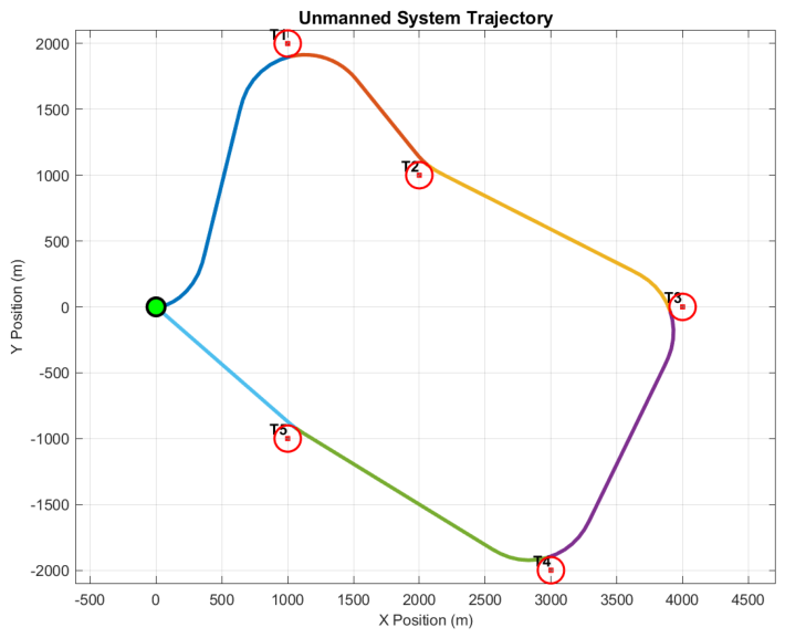
The optimal trajectory obtained under disturbance-free conditions is shown in Figure 1. It can be observed that, in the absence of stochastic disturbances, the UAV accurately reaches each site, i.e., the distance to the corresponding site at each arrival instant satisfies the effective delivery radius constraint.

The above result represents the baseline performance under ideal conditions. In practical mission environments, however, stochastic disturbances are inevitable. To analyze the impact of these parameters on mission success rates, three groups of disturbance parameters with distinct statistical characteristics are configured, as detailed in Table 4. Note that in all parameter sets the disturbances are assumed to be temporally uncorrelated (white noise); only the spatial correlation between the x and y components is varied through the off-diagonal terms of ${\Sigma }_{m,c}$. For each parameter set, $1\times {10}^5$ disturbance sample paths are generated according to the specified statistics, and the success rates for individual sites as well as for the overall mission are evaluated.

Table 4. Disturbance parameter settings.

Parameter	Mean	Support Set	Covariance	Characteristics
Parameter 1	$\left[3.0;4.0\right]$	$\left[1.8,4.2\right]\times \left[2.8,5.2\right]$	$\left[\begin{array}{cc}0.25& 0\\ 0& 0.25\end{array}\right]$	Oblique wind, small variance
Parameter 2	$\left[3.0;4.0\right]$	$\left[1.0,5.0\right]\times \left[2.0,6.0\right]$	$\left[\begin{array}{cc}0.6& 0\\ 0& 0.6\end{array}\right]$	Oblique wind, increased variance
Parameter 3	$\left[3.0;4.0\right]$	$\left[1.0,5.0\right]\times \left[2.5,5.5\right]$	$\left[\begin{array}{cc}0.6& 0.48\\ 0.48& 0.6\end{array}\right]$	Oblique wind, with correlation

Table 4. Disturbance parameter settings.

Parameter	Mean	Support Set	Covariance	Characteristics
Parameter 1	$\left[3.0;4.0\right]$	$\left[1.8,4.2\right]\times \left[2.8,5.2\right]$	$\left[\begin{array}{cc}0.25& 0\\ 0& 0.25\end{array}\right]$	Oblique wind, small variance
Parameter 2	$\left[3.0;4.0\right]$	$\left[1.0,5.0\right]\times \left[2.0,6.0\right]$	$\left[\begin{array}{cc}0.6& 0\\ 0& 0.6\end{array}\right]$	Oblique wind, increased variance
Parameter 3	$\left[3.0;4.0\right]$	$\left[1.0,5.0\right]\times \left[2.5,5.5\right]$	$\left[\begin{array}{cc}0.6& 0.48\\ 0.48& 0.6\end{array}\right]$	Oblique wind, with correlation

As evident from

Table 5. Task completion performance under stochastic disturbances without robust optimization.

Parameter	Performance per Site					Performance Evaluation Across Samples
Parameter 1	Site	Success rate	Mean distance	Std.	Maximum	Overall success rate	0.721%
	Site 1	49.388%	100.061	3.913	117.647	Mean max. distance	105.715
	Site 2	49.313%	100.097	4.297	119.112	Std. dev. of max. distance	3.394
	Site 3	48.929%	100.137	4.990	125.074	90th percentile of sample max. distance	109.908
	Site 4	48.932%	100.158	5.470	129.303	95th percentile of sample max. distance	111.924
	Site 5	49.215%	100.150	5.440	136.582	98th percentile of sample max. distance	114.891
Parameter 2	Site	Success rate	Mean distance	Std.	Maximum	Overall success rate 0.702%
	Site 1	48.874%	100.163	6.048	127.240	Mean max. distance	108.912
	Site 2	48.885%	100.235	6.632	130.809	Std. dev. of max. distance	5.295
	Site 3	48.679%	100.281	7.738	136.902	90th percentile of sample max. distance	115.415
	Site 4	48.333%	100.367	8.450	146.445	95th percentile of sample max. distance	118.714
	Site 5	48.256%	100.381	8.411	149.860	98th percentile of sample max. distance	123.453
Parameter 3	Site	Success rate	Mean distance	Std.	Maximum	Overall success rate	0.520%
	Site 1	49.211%	100.271	4.981	124.177	Mean max. distance	111.279
	Site 2	49.900%	100.035	9.416	143.267	Std. dev. of max. distance	7.737
	Site 3	49.290%	100.276	10.432	152.413	90th percentile of sample max. distance	121.320
	Site 4	48.313%	100.691	7.475	146.074	95th percentile of sample max. distance	126.452
	Site 5	49.831%	100.060	14.333	171.581	98th percentile of sample max. distance	133.203

, when stochastic disturbances are present, if the UAV continues to apply the control law derived from the disturbance-free planning, the probability that it remains within the effective delivery radius at the arrival instant drops substantially. For an individual sample, the likelihood of successfully servicing all five sites is virtually zero. This observation clearly indicates that deterministic planning which neglects stochastic disturbances is inadequate for ensuring mission success in realistic environments.

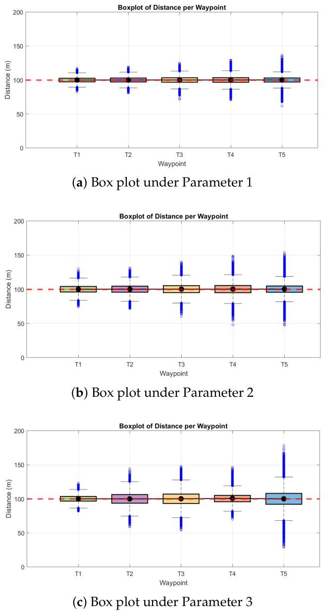
To visually corroborate the statistical findings in Table 5, Figure 2 depicts the corresponding distributions of arrival-to-site distances via box plots. In each subplot, the central mark indicates the median, the box bounds the interquartile range (IQR; i.e., the 25th to 75th percentiles), and the whiskers extend to the most extreme data points not considered outliers. Outliers (distances exceeding approximately $1.5\times \mathrm{IQR}$ from the box) are plotted individually.

As can be observed, under all three disturbance parameter configurations, the median distances cluster tightly around 100 m, which is the effective delivery radius ${\epsilon }_m$ set for the UAV. The relatively narrow IQRs indicate that deterministic planning does nominally guide the UAV to the vicinity of the sites. However, a significant number of outliers extend far beyond 100 m, with some exceeding 130 m (e.g., under Parameter 3). These outliers directly correspond to the failed delivery attempts, wherein the stochastic disturbance perturbs the UAV sufficiently to violate the waypoint constraint. The figure thus provides direct visual evidence that, without robustness considerations, the UAV’s arrival positions are highly sensitive to random disturbances.

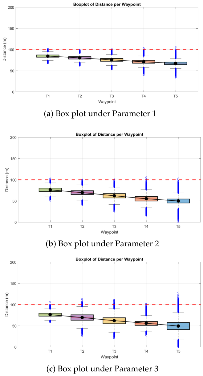
To address this issue, the proposed distributionally robust optimization model is employed. First, the safety margins corresponding to each waypoint are computed using the algorithm described previously. The robust optimal control model is then solved to obtain the optimal trajectory that accounts for the influence of disturbances. The success rates under the robust optimization scheme are reported in

Table 6. Task completion performance under stochastic disturbances with robust optimization.

Parameter	Performance per Site					Performance Evaluation Across Samples
Parameter 1	Site	Success rate	Mean distance	Std.	Maximum	Overall success rate	99.989%
	Site 1	99.994%	84.660	3.933	102.026	Mean max. distance	86.091
	Site 2	100.000%	80.550	4.305	98.999	Std. dev. of max. distance	3.022
	Site 3	100.000%	75.683	5.030	98.908	90th percentile of sample max. distance	90.139
	Site 4	99.998%	71.171	5.519	102.112	95th percentile of sample max. distance	91.497
	Site 5	99.997%	67.492	5.473	105.474	98th percentile of sample max. distance	93.073
Parameter 2	Site	Success rate	Mean distance	Std.	Maximum	Overall success rate	99.988%
	Site 1	99.995%	76.239	6.108	101.455	Mean max. distance	78.487
	Site 2	100.000%	69.963	6.668	99.364	Std. dev. of max. distance	4.699
	Site 3	99.998%	62.374	7.782	102.506	90th percentile of sample max. distance	84.776
	Site 4	99.997%	55.506	8.562	103.758	95th percentile of sample max. distance	86.906
	Site 5	99.998%	50.280	8.459	100.815	98th percentile of sample max. distance	89.383
Parameter 3	Site	Success rate	Mean distance	Std.	Maximum	Overall success rate	99.668%
	Site 1	99.998%	76.382	5.131	102.959	Mean max. distance	79.574
	Site 2	99.903%	69.609	9.634	110.142	Std. dev. of max. distance	5.023
	Site 3	99.923%	62.232	10.676	117.931	90th percentile of sample max. distance	88.039
	Site 4	99.994%	56.134	7.579	105.543	95th percentile of sample max. distance	88.729
	Site 5	99.832%	49.458	14.520	132.344	98th percentile of sample max. distance	92.363

, and the corresponding distance box plots are shown in Figure 3.

The simulation results demonstrate that the optimal trajectories generated by the proposed robust optimal control model effectively mitigate the adverse effects of stochastic disturbances. The service success rates for individual sites, as well as the overall mission success rate per trial, consistently exceed 90%. These outcomes corroborate the effectiveness of the proposed method in handling stochastic disturbances.

Although the robust optimal control model guarantees the required probabilistic reachability, this reliability comes at a price: the safety margins force the nominal trajectory to stay closer to the sites, which could potentially increase the total flight time. To quantify this trade-off, we compare the total mission times of the deterministic and robust trajectories for the five-site scenario under disturbance Parameter 3 (Table 4). The deterministic planning (safety margin zero) yields a total time of $239.87$ s, while the robust planning with $\delta =0.1$ requires $243.71$ s. The increase is merely $3.84$ s, i.e., a relative increase of about $1.6\%$.

The modest time penalty is due to the fact that the required safety margins are on the order of 10–50 for the mean distances. The additional maneuvering to satisfy the margin constraints is therefore negligible. These results demonstrate that the proposed framework can achieve extremely high mission success rates while preserving almost the same mission efficiency as the deterministic baseline. If a more stringent reliability (smaller $\delta$) is required, the safety margins would grow, leading to a more noticeable time increase; this inherent trade-off can be directly managed by the mission planner through the choice of $\delta$.

In terms of computational cost, a single robust trajectory planning (the second stage of the two-stage method) requires approximately $0.8$ s on a standard desktop computer (Intel Core i7-12700H, 32 GB RAM, MATLAB R2023a). The safety margins are precomputed offline via the semidefinite program and stored in a two-dimensional lookup table; the online retrieval and linear interpolation add negligible overhead. The computational overhead of the robust extension compared to deterministic planning is minimal, because the safety margins are retrieved from the precomputed lookup table rather than solved online.

5.1.2. Impact of Disturbance Parameter Settings on Delivery Effectiveness

To further investigate the influence of different disturbance characteristics on the delivery effectiveness of the UAV, this subsection designs multiple groups of disturbance parameters with distinct statistical properties, as detailed in

Table 7. Settings of different disturbance parameters.

Parameter	Mean	Support Set	Covariance	Characteristics
Parameter 1	$\left[0;0\right]$	$\left[-1.2,1.2\right]\times \left[-1.2,1.2\right]$	$\left[\begin{array}{cc}0.25& 0\\ 0& 0.25\end{array}\right]$	Light wind, zero mean
Parameter 2	$\left[3.0;0\right]$	$\left[1.8,4.2\right]\times \left[-1.2,1.2\right]$	$\left[\begin{array}{cc}0.25& 0\\ 0& 0.25\end{array}\right]$	Unidirectional wind introduced
Parameter 3	$\left[3.0;0\right]$	$\left[1.0,5.0\right]\times \left[-2.0,2.0\right]$	$\left[\begin{array}{cc}0.25& 0\\ 0& 0.25\end{array}\right]$	Enlarged support set
Parameter 4	$\left[3.0;0\right]$	$\left[1.0,5.0\right]\times \left[-2.0,2.0\right]$	$\left[\begin{array}{cc}0.6& 0\\ 0& 0.6\end{array}\right]$	Increased covariance
Parameter 5	$\left[3.0;4.0\right]$	$\left[1.0,5.0\right]\times \left[2.0,6.0\right]$	$\left[\begin{array}{cc}0.6& 0\\ 0& 0.6\end{array}\right]$	Increased covariance
Parameter 6	$\left[3.0;4.0\right]$	$\left[1.0,5.0\right]\times \left[2.0,6.0\right]$	$\left[\begin{array}{cc}0.6& 0.24\\ 0.24& 0.6\end{array}\right]$	Positive correlation introduced
Parameter 7	$\left[3.0;4.0\right]$	$\left[1.0,5.0\right]\times \left[2.5,5.5\right]$	$\left[\begin{array}{cc}0.6& 0.24\\ 0.24& 0.6\end{array}\right]$	Reduced support set
Parameter 8	$\left[3.0;4.0\right]$	$\left[1.0,5.0\right]\times \left[2.5,5.5\right]$	$\left[\begin{array}{cc}0.6& 0.48\\ 0.48& 0.6\end{array}\right]$	Enhanced correlation
Parameter 9	$\left[3.0;-4.0\right]$	$\left[1.0,5.0\right]\times \left[-5.5,-2.5\right]$	$\left[\begin{array}{cc}0.6& -0.48\\ -0.48& 0.6\end{array}\right]$	Negative correlation
Parameter 10	$\left[3.0;-4.0\right]$	$\left[1.0,5.0\right]\times \left[-5.5,-2.5\right]$	$\left[\begin{array}{cc}0.7& -0.48\\ -0.48& 0.5\end{array}\right]$	Unequal variances with equal sum
Parameter 11	$\left[3.0;-4.0\right]$	$\left[1.0,5.0\right]\times \left[-5.5,-2.5\right]$	$\left[\begin{array}{cc}0.8& -0.48\\ -0.48& 0.4\end{array}\right]$	Unequal variances with equal sum
Parameter 12	$\left[3.0;-4.0\right]$	$\left[1.0,5.0\right]\times \left[-5.5,-2.5\right]$	$\left[\begin{array}{cc}0.4& -0.48\\ -0.48& 0.8\end{array}\right]$	Unequal variances with equal sum

. Specifically: Parameter Sets 1 through 4 primarily simulate unidirectional wind disturbances. Set 2 alters the mean magnitude relative to Set 1; Set 3 expands the support set compared to Set 2; and Set 4 further increases the variance relative to Set 3. Parameter Sets 5 through 12 simulate diagonal wind disturbances with varying directions and correlations. Set 5 introduces a non-zero mean along the vertical axis based on Set 4, thereby forming a diagonal wind. Set 6 further introduces positive correlation between the disturbance components. Set 7 adjusts the support set size. Set 8 strengthens the correlation magnitude. Set 9 alters the wind direction and changes the correlation from positive to negative. Sets 10 through 12 maintain a constant sum of variances in both directions while varying the individual variance allocations.

Under each of the above disturbance parameter configurations, the trajectories generated by the proposed distributionally robust optimal control method ensure that the arrival positions of the UAV fall within the effective delivery radius with a probability no less than the prescribed level, preliminarily validating the robustness of the method in stochastic environments. To quantitatively characterize the impact of disturbance parameters on mission effectiveness, the overall statistical properties of the distances at arrival instants for all sites (

Table 8. Statistical characteristics of distances at arrival moments across all sites.

Statistic	Parameter 1	Parameter 2	Parameter 3	Parameter 4	Parameter 5	Parameter 6
Total observations	100,000	100,000	100,000	100,000	100,000	100,000
Global mean distance (m)	75.666	75.843	75.834	62.700	62.872	62.934
Std. dev. (m)	7.779	7.746	7.734	11.951	12.079	13.215
Minimum distance (m)	30.748	28.366	31.939	4.766	4.228	1.145
Maximum distance (m)	104.102	104.212	102.637	104.066	103.758	115.876
Median distance (m)	75.819	76.090	76.103	63.068	63.280	63.640
Violation count	22	17	17	12	12	96
Violation rate	0.004%	0.003%	0.003%	0.002%	0.002%	0.019%
Statistic	Parameter 7	Parameter 8	Parameter 9	Parameter 10	Parameter 11	Parameter 12
Total observations	100,000	100,000	100,000	100,000	100,000	100,000
Global mean distance (m)	62.528	62.763	62.790	62.833	62.891	62.802
Std. dev. (m)	13.198	13.820	11.458	11.261	11.127	11.955
Minimum distance (m)	0.412	0.487	11.408	14.795	21.351	5.590
Maximum distance (m)	112.632	132.344	125.102	118.819	123.785	121.898
Median distance (m)	63.528	63.218	63.893	64.032	64.240	63.810
Violation count	98	350	260	152	136	548
Violation rate	0.020%	0.070%	0.052%	0.030%	0.027%	0.110%

“violation” means a single site failing.

), the statistical properties of the maximum distance per trial (

Table 9. Statistical characteristics of the maximum distance at arrival moments across samples.

Statistic	Parameter 1	Parameter 2	Parameter 3	Parameter 4	Parameter 5	Parameter 6
Overall success rate	99.978%	99.983%	99.984%	99.988%	99.988%	99.908%
Mean max. distance	85.797	85.861	85.826	78.167	78.487	79.198
Std. dev.	3.199	3.148	3.137	4.883	4.699	4.805
90th percentile	90.102	90.084	90.074	84.740	84.776	85.538
95th percentile	91.577	91.511	91.476	87.000	86.906	87.804
98th percentile	93.288	93.186	93.158	89.531	89.383	90.542
Statistic	Parameter 7	Parameter 8	Parameter 9	Parameter 10	Parameter 11	Parameter 12
Overall success rate	99.903%	99.668%	99.742%	99.850%	99.873%	99.460%
Mean max. distance	79.134	79.574	77.356	77.071	76.845	78.039
Std. dev.	4.797	5.023	6.084	5.867	5.755	6.571
90th percentile	85.433	88.039	85.839	85.267	84.795	87.254
95th percentile	87.674	88.729	89.034	88.248	87.727	90.759
98th percentile	90.444	92.363	92.547	91.821	91.081	94.819

), and the detailed statistics for each individual site (

Table 10. Detailed statistical characteristics of distances at arrival moments for each site.

Parameter	Performance per Site						Distribution per Site
1	Site	Success rate	Mean	Std. dev.	Maximum	Safety margin	5%	25%	50%	75%	90%	95%	99%	Range
	Site 1	99.986%	84.074	4.273	104.102	15.926	77.048	81.195	84.056	86.958	89.544	91.127	94.009	16.961
	Site 2	99.998%	80.136	4.578	102.123	19.864	72.601	77.072	80.124	83.201	85.968	87.652	90.905	18.304
	Site 3	99.999%	75.251	5.262	101.456	24.749	66.655	71.804	75.253	78.712	81.860	83.883	87.867	21.212
	Site 4	99.999%	71.211	5.535	100.921	28.789	62.340	67.717	71.164	74.665	78.000	80.213	85.231	22.891
	Site 5	99.996%	67.656	5.492	104.004	32.344	59.217	64.598	67.590	70.629	73.770	76.313	83.572	24.355
2	Site	Success rate	Mean	Std. dev.	Maximum	Safety margin	5%	25%	50%	75%	90%	95%	99%	Range
	Site 1	99.992%	84.130	4.217	103.046	15.870	77.185	81.281	84.134	86.981	89.543	91.054	93.954	16.769
	Site 2	99.998%	80.321	4.520	100.275	19.679	72.926	77.281	80.297	83.343	86.129	87.788	90.935	18.009
	Site 3	99.999%	75.684	5.101	101.105	24.316	67.362	72.326	75.684	79.034	82.113	83.980	87.914	20.552
	Site 4	99.999%	71.447	5.471	100.397	28.553	62.684	68.005	71.415	74.839	78.169	80.386	85.312	22.628
	Site 5	99.995%	67.632	5.504	104.213	32.368	59.180	64.532	67.555	70.636	73.857	76.414	83.417	24.237
3	Site	Success rate	Mean	Std. dev.	Maximum	Safety margin	5%	25%	50%	75%	90%	95%	99%	Range
	Site 1	99.993%	84.126	4.201	102.060	15.874	77.238	81.274	84.126	86.954	89.530	91.059	93.883	16.645
	Site 2	99.999%	80.315	4.481	101.157	19.685	72.910	77.326	80.306	83.315	86.024	87.686	90.824	17.914
	Site 3	99.997%	75.674	5.089	100.876	24.326	67.364	72.313	75.681	79.033	82.098	84.003	87.743	20.379
	Site 4	99.997%	71.441	5.447	101.779	28.559	62.661	68.010	71.409	74.849	78.134	80.308	85.162	22.501
	Site 5	99.997%	67.615	5.480	102.637	32.385	59.128	64.534	67.565	70.642	73.794	76.275	83.350	24.222
4	Site	Success rate	Mean	Std. dev.	Maximum	Safety margin	5%	25%	50%	75%	90%	95%	99%	Range
	Site 1	99.991%	75.532	6.537	104.066	24.468	64.777	71.111	75.549	79.946	83.913	86.297	90.678	25.901
	Site 2	100.000%	69.568	6.984	99.646	30.432	58.076	64.867	69.565	74.258	78.505	81.071	85.901	27.825
	Site 3	99.999%	62.435	7.920	101.749	37.565	49.550	57.813	62.432	67.632	72.415	75.451	81.511	31.961
	Site 4	99.999%	55.872	8.481	100.936	44.128	42.307	50.500	55.795	61.140	66.220	69.660	77.778	35.471
	Site 5	99.999%	50.095	8.401	100.267	49.905	37.364	45.233	49.884	54.661	59.647	63.760	74.527	37.163
5	Site	Success rate	Mean	Std. dev.	Maximum	Safety margin	5%	25%	50%	75%	90%	95%	99%	Range
	Site 1	99.995%	76.239	6.108	101.455	23.761	66.188	72.124	76.261	80.374	84.045	86.277	90.393	24.205
	Site 2	100.000%	69.963	6.668	99.364	30.037	59.008	65.489	69.952	74.447	78.525	80.951	85.689	26.681
	Site 3	99.998%	62.374	7.782	102.506	37.626	49.634	57.278	62.363	67.475	72.184	75.095	81.121	31.487
	Site 4	99.997%	55.506	8.562	103.758	44.494	41.891	50.056	55.401	60.823	66.030	69.464	77.692	35.801
	Site 5	99.998%	50.280	8.459	100.815	49.720	37.537	45.420	50.051	54.748	59.801	64.116	75.351	37.814
6	Site	Success rate	Mean	Std. dev.	Maximum	Safety margin	5%	25%	50%	75%	90%	95%	99%	Range
	Site 1	99.991%	76.347	5.711	103.223	23.653	67.022	72.480	76.296	80.148	83.685	85.861	89.876	22.854
	Site 2	99.983%	69.799	8.417	107.996	30.201	55.973	64.187	69.792	75.421	80.523	83.622	89.535	33.562
	Site 3	99.984%	62.398	9.722	111.952	37.602	46.522	56.024	62.305	68.721	74.724	78.453	86.099	39.577
	Site 4	99.997%	55.887	8.848	100.660	44.113	41.775	50.253	55.642	61.261	66.946	70.874	78.861	37.086
	Site 5	99.949%	50.237	12.596	115.876	49.763	29.419	43.099	50.032	57.124	65.516	71.930	84.191	54.772
7	Site	Success rate	Mean	Std. dev.	Maximum	Safety margin	5%	25%	50%	75%	90%	95%	99%	Range
	Site 1	99.998%	76.341	5.714	102.234	23.659	67.021	72.434	76.280	80.186	83.766	85.794	89.874	22.853
	Site 2	99.976%	69.769	8.339	108.354	30.231	56.031	64.210	69.781	75.339	80.374	83.447	89.275	33.244
	Site 3	99.977%	62.367	9.563	108.644	37.633	46.814	56.073	62.305	68.572	74.436	78.175	85.917	39.103
	Site 4	100.000%	55.877	8.794	98.952	44.123	41.935	50.284	55.645	61.174	66.874	70.810	78.954	37.019
	Site 5	99.951%	49.897	12.388	112.632	50.103	29.578	42.884	49.614	56.632	64.881	71.265	83.540	53.962
8	Site	Success rate	Mean	Std. dev.	Maximum	Safety margin	5%	25%	50%	75%	90%	95%	99%	Range
	Site 1	99.998%	76.382	5.131	102.959	23.618	68.329	72.814	76.174	79.704	83.123	85.176	89.240	20.911
	Site 2	99.903%	69.609	9.634	110.142	30.391	53.725	63.154	69.628	76.040	81.938	85.468	92.123	38.398
	Site 3	99.923%	62.232	10.676	117.931	27.768	45.008	55.114	62.046	69.136	75.806	80.198	88.556	43.548
	Site 4	99.994%	56.134	7.579	105.543	43.866	45.181	51.096	55.373	60.312	65.834	69.830	78.467	33.286
	Site 5	99.832%	49.458	14.520	132.344	50.542	24.958	41.185	49.241	57.427	67.285	74.416	87.986	63.028
9	Site	Success rate	Mean	Std. dev.	Maximum	Safety margin	5%	25%	50%	75%	90%	95%	99%	Range
	Site 1	99.843%	74.515	8.269	109.888	25.485	61.176	68.809	74.371	80.072	85.237	88.373	94.212	33.036
	Site 2	100.000%	69.478	3.677	88.625	30.522	63.550	66.991	69.418	71.883	74.169	75.594	78.459	14.909
	Site 3	99.998%	62.653	6.326	110.478	37.347	53.208	58.328	62.142	66.419	70.821	73.798	80.084	26.876
	Site 4	99.899%	56.023	11.742	125.102	43.977	37.271	48.343	55.636	63.259	70.825	75.913	86.756	49.485
	Site 5	100.000%	51.283	6.023	98.470	48.717	42.872	47.679	50.560	54.013	58.789	62.370	70.311	27.439
10	Site	Success rate	Mean	Std. dev.	Maximum	Safety margin	5%	25%	50%	75%	90%	95%	99%	Range
	Site 1	99.914%	74.594	7.730	110.110	25.406	62.264	69.242	74.375	79.729	84.646	87.636	93.391	31.127
	Site 2	100.000%	69.492	3.445	87.761	30.508	63.926	67.183	69.441	71.761	73.914	75.192	77.788	13.862
	Site 3	99.998%	62.559	7.015	103.573	37.441	52.076	57.676	61.979	66.826	71.676	74.997	81.720	29.644
	Site 4	99.936%	56.201	11.067	118.819	43.799	38.757	48.819	55.765	62.938	70.271	75.220	85.668	46.911
	Site 5	100.000%	51.320	5.613	94.459	48.680	43.496	47.991	50.625	53.816	58.418	61.794	68.913	25.417
11	Site	Success rate	Mean	Std. dev.	Maximum	Safety margin	5%	25%	50%	75%	90%	95%	99%	Range
	Site 1	99.948%	74.641	7.224	108.761	25.359	63.171	69.619	74.380	79.405	84.077	86.997	92.408	29.237
	Site 2	100.000%	69.505	3.248	86.568	30.495	64.410	67.317	69.376	71.549	73.636	75.020	78.003	13.593
	Site 3	99.984%	62.529	7.785	117.320	37.471	50.991	57.037	61.876	67.311	72.768	76.305	83.687	32.696
	Site 4	99.933%	56.337	10.558	123.785	43.663	40.167	49.138	55.649	62.689	69.905	74.848	85.465	45.298
	Site 5	99.999%	51.443	5.323	104.989	48.557	44.313	48.253	50.655	53.700	58.166	61.392	68.815	24.502
12	Site	Success rate	Mean	Std. dev.	Maximum	Safety margin	5%	25%	50%	75%	90%	95%	99%	Range
	Site 1	99.639%	74.425	9.278	116.155	25.575	59.260	68.132	74.321	80.641	86.363	89.846	96.484	37.224
	Site 2	100.000%	69.474	4.118	97.272	30.526	63.319	66.639	69.146	71.939	74.825	76.779	80.807	17.488
	Site 3	100.000%	62.873	4.655	97.302	37.127	56.074	59.749	62.459	65.492	68.790	71.176	76.403	20.329
	Site 4	99.821%	55.800	13.542	121.898	44.200	33.677	47.057	55.572	64.251	72.885	78.699	90.139	56.462
	Site 5	99.992%	51.437	6.978	105.311	48.563	42.340	47.117	50.295	54.454	60.090	64.789	75.026	32.686

) are compiled. A systematic analysis of these statistical results yields the following key observations.

1. Influence of Site Order Under a Given Disturbance Parameter Set.

As shown in Table 10, for any given disturbance parameter set, the mean distance between the UAV and the site at the arrival instant exhibits a monotonic decreasing trend as the service sequence proceeds from Site 1 to Site 5. Taking Parameter Set 1 as an example, the average distances for Site 1 through 5 are 84.07 m, 80.14 m, 75.25 m, 71.21 m, and 67.66 m, respectively; under Parameter Set 4, the corresponding values are 69.57 m, 62.44 m, 55.87 m, 50.10 m. This phenomenon arises because the accumulation of mission execution time leads to progressively larger position uncertainty. To maintain the reliability of the waypoint constraints, the required safety margin must increase accordingly, forcing the nominal trajectory closer to the sites and ultimately resulting in a reduction in the mean arrival distance. The standard deviations of the distances at each site, however, are closely related to the directional characteristics of the disturbance and do not strictly vary monotonically with the site order (e.g., under Parameter Set 4, the standard deviations for Sites 3 to 5 are 7.92, 8.48, and 8.40, respectively), reflecting the directional heterogeneity in the accumulation of uncertainty.

2. Impact of Disturbance Parameter Variations on Arrival Distance Distribution.

(1) Influence of Variance Magnitude.

Comparing the results of Parameter Sets 1–3 with those of Set 4 in Table 10 reveals that as the disturbance variance increases, the mean arrival distances at all sites decrease notably. For Site 1, the mean distance drops from 84.07 m under Set 1 to 75.53 m under Set 4; for Site 5, it decreases from 67.66 m to 50.10 m. Concurrently, the standard deviations at each site increase significantly: the standard deviation for Site 1 rises from 4.27 m to 6.54 m, and for Site 5 from 5.49 m to 8.40 m. This indicates that enhanced uncertainty due to larger variance leads to a more dispersed distribution of arrival distances. The minor differences in variance among Sets 1–3 correspond to nearly identical mean distances and standard deviations, further corroborating the dominant role of variance.

(2) Introduction of Diagonal Wind (Two-Dimensional Disturbance).

A comparison between Parameter Sets 4 and 5 demonstrates that, under identical support set and covariance matrix conditions, the introduction of a diagonal wind with a non-zero mean has a negligible effect on the arrival distance distributions. For Site 1, the mean distance changes from 75.53 m to 76.24 m, and the standard deviation from 6.54 m to 6.11 m; for Site 5, the mean distance changes from 50.10 m to 50.28 m, and the standard deviation from 8.40 to 8.46. Thus, the direction of the disturbance mean exerts limited influence on the arrival distance distribution, whereas the second-order moment characteristics are the determining factor.

(3) Influence of Disturbance Correlation.

A comparison between Parameter Sets 5 and 6 reveals that the impact of correlation on the arrival distance distribution is broadening or narrowing, and exhibits complex variations depending on the site order.

Site 1: The mean distance remains essentially unchanged; the standard deviation decreases from 6.11 m to 5.71 m; the 5th percentile rises from 66.19 m to 67.02 m; and the 95th percentile drops from 86.28 m to 85.86 m, indicating a more concentrated distribution.

Site 2: The mean distance remains essentially unchanged; the standard deviation increases from 6.67 m to 8.42 m; the 5th percentile drops from 59.01 m to 55.97 m; and the 95th percentile rises from 80.95 m to 83.62 m, indicating a more dispersed distribution.

Site 5: The mean distance remains essentially unchanged; the standard deviation increases markedly from 8.46 m to 12.60 m; the 5th percentile drops from 37.54 m to 29.42 m; and the 95th percentile rises from 64.12 m to 71.93 m, indicating a substantially more dispersed distribution.

These results suggest that increased correlation alters the propagation of uncertainty along the task sequence, and its effect is closely coupled with both the accumulated time and the disturbance direction, exhibiting non-uniform behavior across different sites. Parameter Set 8, which further strengthens the positive correlation relative to Set 7, also shows inconsistent trends across sites: the standard deviation for Site 1 decreases from 5.71 m to 5.13 m (more concentrated), while that for Site 5 increases from 12.39 m to 14.52 m (more dispersed), further corroborating this characteristic.

To understand this non-monotonic, site-dependent behavior theoretically, it is instructive to examine the spectral decomposition of the disturbance covariance matrix. For Parameter Set 6, the covariance matrix is ${\Sigma }_{m,c}=\left[\begin{array}{cc}0.6& 0.24\\ 0.24& 0.6\end{array}\right]$, whose eigenvalues are ${\lambda }_{\max }=0.84$ and ${\lambda }_{\min }=0.36$, with corresponding eigenvectors ${\mathit{v}}_{\max }={\displaystyle \frac{1}{\sqrt{2}}}{[1,1]}^T$ (the direction of maximum uncertainty, oriented at 45°) and ${\mathit{v}}_{\min }={\displaystyle \frac{1}{\sqrt{2}}}{[1,-1]}^T$ (the direction of minimum uncertainty, oriented at −45°). The position deviation covariance inherits this eigenstructure, scaled by the accumulated time: $\mathrm{Cov}\left({\mathit{p}}^{\mathrm{dev}}\right)=T_{i,K}\Sigma$.

The segment travel direction determines how uncertainty projects onto the arrival distance. Specifically, the variance in the position deviation along the direction of travel between consecutive sites is given by ${\mathit{u}}^T\Sigma \mathit{u}$, where $\mathit{u}$ is the unit vector of the segment. For Segment $1\to 2$ (from Site 1 at $(1000,2000)$ to Site 2 at $(2000,1000)$), the travel direction is ${\mathit{u}}_{1\to 2}={\displaystyle \frac{1}{\sqrt{2}}}{[1,-1]}^T$, which coincides exactly with ${\mathit{v}}_{\min }$. Consequently, the uncertainty along this segment is governed by the smaller eigenvalue ${\lambda }_{\min }=0.36$, leading to a more concentrated distribution of the position deviation and hence a narrower arrival distance spread at Site 2 when correlation is introduced (compared to the isotropic case). In contrast, for Segment $4\to 5$ (from $(3000,-2000)$ to $(1000,-1000)$), ${\mathit{u}}_{4\to 5}={\displaystyle \frac{1}{\sqrt{5}}}{[-2,1]}^T$, which forms a large angle with ${\mathit{v}}_{\min }$ and has a substantial projection onto ${\mathit{v}}_{\max }$, thereby increasing the effective variance and leading to a more dispersed arrival distance distribution at Site 5.

More generally, the non-monotonic site dependence arises from the interplay between (i) the alignment or misalignment of each segment’s travel direction with the eigenvectors of the covariance matrix, which dictates the effective variance along that direction, and (ii) the linear accumulation of uncertainty over time ($T_{i,K}$), which progressively amplifies these directional effects for later sites. When correlation is introduced, the eigenvectors rotate away from the coordinate axes, and the anisotropy of the uncertainty ellipsoid causes the arrival distance distribution to be alternately broadened or narrowed depending on the specific geometry of each segment, producing the complex site-dependent patterns observed in Table 8 and Table 10.

(4) Influence of Support Set.

Comparisons between Parameter Sets 6 and 7, as well as between Sets 2 and 3, indicate that under fixed mean and covariance, altering the support set size has virtually no impact on the arrival distance distributions. For instance, under Sets 6 and 7, the mean distances for Site 1 are 76.35 m and 76.34 m, respectively, with a standard deviation of 5.71 m in both cases; for Site 5, the mean distances are 50.24 m and 49.90 m, with standard deviations of 12.60 m and 12.39 m. This observation confirms that once the moment information is specified, the boundaries of the support set exert negligible influence on the worst-case probability constraint, which is fully consistent with the theoretical derivation that relies solely on moment information for constraint reformulation.

(5) Influence of Variance Allocation (Constant Sum).

In Table 10, Parameter Sets 9 through 12 maintain a constant sum of variances in both directions while varying the individual allocation proportions. The data reveal that the allocation of variances does affect the distribution of arrival distances at each site, yet the effect is not uniform across different sites. For Site 1, the standard deviations under Sets 9, 11, and 12 are 8.27 m, 7.22 m, and 9.28 m, respectively, exhibiting a decreasing-then-increasing trend; in contrast, for Site 3, the corresponding standard deviations are 6.33 m, 7.79 m, and 4.66 m, showing an increasing-then-decreasing pattern. Meanwhile, the mean arrival distances for each site remain largely stable (Site 1: 74.52 m, 74.64 m, 74.43 m; Site 3: 62.23 m, 62.53 m, 62.87 m). These observations indicate that, under a fixed total level of uncertainty, the allocation of variances between the two axes influences the spread of arrival distances in a manner that is closely coupled with both the site order and the specific parameter combination, reflecting a certain degree of complexity.

3. Overall Success Rate Analysis.

The statistical properties of individual trials (Table 9) reveal that the overall mission success rates under all parameter configurations exceed 99.4%, with corresponding violation rates below 0.1%, demonstrating that the proposed method effectively controls the risk level during mission execution. The mean values of the maximum arrival distance across all sites within a single trial exhibit the following trends with respect to disturbance parameter variations: as the disturbance variance increases (e.g., from Parameter Sets 1–3 to Set 4), the mean maximum distance decreases notably, indicating that the nominal trajectory is forced closer to the sites to satisfy the probabilistic constraints. In contrast, the influence of enhanced correlation (e.g., comparing Set 5 with Set 6 or Set 7 with Set 8) on this mean value is more intricate, showing both increases and decreases depending on the specific parameter combination, which reflects the modulating effect of correlation on the propagation of uncertainty. This non-monotonicity is a direct consequence of the eigenvector-segment alignment mechanism discussed above: because the effective variance alternates between being enlarged or suppressed segment-by-segment based on the local travel geometry, the overall maximum distance across all sites reflects a mixture of these competing effects, with the dominant contribution often arising from the segment where the travel direction is most closely aligned with ${\mathit{v}}_{\max }$.

In summary, the statistical characteristics of the arrival distance between the UAV and the sites are primarily influenced by the disturbance variance and the correlation between disturbance components, whereas the roles of the disturbance mean and the support set boundaries are relatively minor. Notably, the impact of correlation on the arrival distance distribution exhibits non-uniform variations across different sites, highlighting the complexity of uncertainty accumulation and propagation along the task sequence. The proposed method, through rational allocation of safety margins among sites within the distributionally robust optimization framework, guarantees mission success across diverse disturbance environments, and the observed statistical regularities are in agreement with the theoretical expectations.

5.1.3. Comparison with Wasserstein-Based Distributionally Robust Optimization

To further benchmark the proposed moment-based distributionally robust optimal control, we implement a competing method using a Wasserstein ambiguity set following the framework of [3]. For a fair comparison, both approaches are employed to compute the minimum safety margin $\gamma$ that guarantees ${\sup }_{\mathbb{P}\in \mathcal{P}}\mathrm{Pr}(\parallel \mathit{\eta }\parallel >\gamma )\le \delta$ ($\delta =0.1$) for the same disturbance parameter set (Parameter 3 in Table 4) and for accumulated flight times T ranging from 10 s to 300 s.

The moment-based method (proposed) constructs $\mathcal{P}$ solely from the disturbance mean $\mathit{\mu }$, covariance upper bound ${\Sigma }_c$, and support set $\Lambda$, and solves the resulting semidefinite program as detailed in Section 3.2.5.

The Wasserstein-based baseline (cf. [3]) draws $L=30$ independent samples of the position deviation $\mathit{\eta }$, builds the empirical distribution ${\widehat{\mathbb{P}}}_L$, and defines the ambiguity set as a 1-Wasserstein ball ${\mathcal{P}}_W=\{\mathbb{P}:W_1(\mathbb{P},{\widehat{\mathbb{P}}}_L)\le \rho \}$. The radius $\rho$ is set according to the finite-sample guarantee $\rho ={(\log \left(q_1{\beta }^{-1}\right)/\left(q_{2}L\right))}^{1/2}$ with $\beta =0.1$, $q_1=1$, and $q_2=0.1$, resulting in $\rho \approx 0.88$. The corresponding distributionally robust chance constraint is conservatively approximated via CVaR and dualized into a tractable convex program [3], and ${\gamma }_W$ is obtained by bisection.

Table 11. Safety margins $\gamma$ computed by the moment-based DRO (proposed approach) and the Wasserstein-based DRO (baseline, cf. [3]) for different accumulated times.

Time (s)	Moment-DRO	Wasserstein-DRO	Time (s)	Moment-DRO	Wasserstein-DRO
10	10.95	16.22	160	43.77	33.16
20	15.48	20.54	170	45.12	41.53
30	18.97	18.93	180	46.35	34.05
40	21.90	23.81	190	47.61	35.69
50	24.48	25.61	200	48.90	41.80
60	26.83	27.25	210	50.09	36.02
70	28.97	28.78	220	51.36	35.22
80	30.93	30.31	230	52.32	48.67
90	32.85	31.72	240	53.67	43.91
100	34.59	33.08	250	54.47	43.56
110	36.31	33.98	260	55.58	38.60
120	37.93	34.97	270	56.92	40.79
130	39.35	35.98	280	57.72	41.98
140	40.94	37.03	290	58.80	49.17
150	42.43	37.11	300	60.00	49.11

reveals a sharp contrast between the two methods. The moment-based margin ${\gamma }_M$ increases monotonically from 10.95 m to 60.00 m, which is physically consistent: as the position-deviation covariance grows linearly with T (Equations (70)–(80)), a larger safety margin is naturally required.

In stark contrast, the Wasserstein-based margin ${\gamma }_W$ exhibits non-monotonic oscillations. For example, ${\gamma }_W$ drops from 20.54 m at $T=20$ s to 18.93 m at $T=30$ s, and from 37.11 m at $T=150$ s to 33.16 m at $T=160$ s, despite the longer exposure to disturbances. Such fluctuations contradict engineering intuition and would be unreliable for mission-critical planning.

This non-monotonicity is an inherent consequence of the data-driven nature of the Wasserstein ambiguity set. The Wasserstein ball is centered at the empirical distribution constructed from only $L=30$ samples, whose ability to represent tail risks varies randomly across different sample batches. When a particular sample set happens to be clustered near the mean, the worst-case distribution within the ball cannot account for large deviations, resulting in an artificially small ${\gamma }_W$; a batch containing more extreme points yields a larger ${\gamma }_W$. Moreover, the radius $\rho$ is determined solely by the sample size and confidence level, not by the magnitude of T, so it does not compensate for the missing tail information when the empirical distribution fails to capture the increased dispersion at larger T.

The moment-based approach, by contrast, is completely sample-free. Its ambiguity set is defined exclusively through the first- and second-order moments and the support set, all of which are deterministic functions of T. Hence ${\gamma }_M$ is not only monotonic but also deterministic and reproducible, providing a consistent safety margin that a mission planner can trust without worrying about the representativeness of a limited historical record.

This comparison substantiates a key advantage of the proposed framework for emergency response: when only summary statistics (mean, covariance, bounds) can be reliably estimated, the moment-based DRO offers a physically coherent, monotonically increasing safety margin, whereas a Wasserstein-based DRO, although potentially less conservative when abundant samples are available, may produce unreliable, non-monotonic results under scarce data.

5.2. Validation of the Bi-Level Task Assignment Optimization Model

5.2.1. Benefit of Tight Bi-Level Coupling: A Comparison with a Decoupled Baseline

To validate the superiority of the integrated “decision–control” model for UAV cooperative task assignment under kinematic constraints, this subsection presents a comparative analysis against the traditional static task assignment model based on Euclidean distance. In the traditional model, assignment decisions are made exclusively based on the straight-line distance between unmanned systems and targets. This approach typically assume that all systems travel at constant maximum speed, thereby neglecting actual kinematic constraints and the trajectory optimization processes.

This subsection considers a scenario in which two UAVs are tasked with servicing multiple relief sites. The specific locations of the relief sites are provided in

Table 12. Specific locations and demand values of the relief sites.

Relief Sites	x	y	Value	Relief Sites	x	y	Value
Relief site 1	−326.00	121.00	98.71	Relief site 7	−252.00	1431.00	93.76
Relief site 2	−471.00	667.00	84.56	Relief site 8	−468.00	824.00	98.78
Relief site 3	−287.00	590.00	94.01	Relief site 9	−252.00	931.00	89.67
Relief site 4	−6.00	500.00	74.26	Relief site 10	35.00	998.00	71.07
Relief site 5	317.00	613.00	82.66	Relief site 11	310.00	891.00	95.47
Relief site 6	442.00	267.00	97.47	Relief site 12	438.00	1239.00	98.01

. The kinematic parameters for the UAVs are set as follows: speed range $\left[10,50\right]\mathrm{m}/\mathrm{s}$, acceleration range $\left[-5,5\right]{\mathrm{m}/\mathrm{s}}^2$, and heading angular rate range $\left[-0.1,0.1\right]\mathrm{rad}/\mathrm{s}$. In the decoupled baseline, the upper-level assignment is first determined by solving a standard MTSP using Euclidean distances as surrogate costs. Subsequently, for each UAV, the assigned sequence is fed into the same deterministic minimum-time optimal control problem (Equation (30) with ${\xi }_m$ = 0) to compute the actual flight time and trajectory.

By comparing the total mission completion time and the total path cost obtained by the two methods in this scenario, the performance limitations of the traditional method, which arise from its disregard for kinematic constraints and trajectory optimization, are clearly revealed. This comparison serves to demonstrate the necessity and advancement of the integrated modeling and optimization approach proposed in this paper.

The traditional task assignment method makes decisions based solely on Euclidean distance. The resulting shortest straight-line paths are shown in Figure 4a. While this assignment appears geometrically efficient, the actual flight trajectories under realistic kinematic constraints (Figure 4b) require frequent heading and speed adjustments. This leads to a significant increase in mission completion time. Specifically, the calculated mission completion times for UAV 1 and UAV 2 are 94.03 s and 100.63 s, respectively.

The task assignment scheme and the corresponding motion trajectories obtained by the integrated model proposed in this paper are shown in Figure 5. Although the total straight-line path length of this scheme is longer than that of the traditional method (detailed comparisons are presented in

Table 13. Comparison of results between the traditional method and the integrated decision–control method.

	Comparison Item	UAV 1	UAV 2
Traditional Task Assignment Method	Assignment Scheme	$1,2,3,4,5,6$	$7,8,9,10,11,12$
	Mission Execution Time	94.03 s	100.63 s
	Total Euclidean Path Length	2633.65	2617.07
Integrated Decision–Control Method	Assignment Scheme	$1,2,9,10,11,6$	$7,8,3,4,5,12$
	Mission Execution Time	66.07 s	66.07 s
	Total Euclidean Path Length	2999.16	2986.10

), the actual mission completion times for both UAVs, while satisfying all kinematic constraints, are significantly reduced to merely 66.07 s. This contrast clearly demonstrates that for a dynamic system, minimal spatial distance does not guarantee optimal temporal efficiency, and that the impact of kinematic constraints on overall performance is crucial. By co-optimizing task assignment and trajectory generation, the integrated “decision–control” approach achieves superior performance in the time domain.

The key metrics of the task assignment schemes obtained by the two methods are compared in Table 13.

Analysis of the assignment schemes and trajectory morphology reveals distinct strategic differences. The traditional method adopts a symmetrical region-partitioning strategy (Figure 4a), assigning targets on the left and right sides to UAV 1 and UAV 2, respectively. While this scheme appears balanced and reasonable when kinematic constraints are ignored, the actual trajectories under constraints (Figure 4b) exhibit frequent, sharp turns for each UAV, which substantially increases the time cost.

In contrast, the integrated model employs a cross-region, interleaved assignment strategy (Figure 5). As indicated in Table 13, this strategy breaks the simple spatial partition, resulting in more spatially dispersed target sequences for each UAV and consequently generating smoother overall trajectories. Its core advantage lies in significantly reducing the cumulative turning demand imposed on any single UAV within a localized area. The essence of this strategy is the implicit consideration of kinematic feasibility at the decision-making stage, thereby achieving a more balanced redistribution of the maneuvering load across the entire multi-UAV.

From the perspective of the underlying optimization mechanism, the traditional decoupled approach fails to account for the dynamic characteristics of the unmanned systems during the task assignment phase. Consequently, the subsequent trajectory planning phase is constrained to passively adapt to the predetermined target sequence, offering limited scope for genuine optimization.

In contrast, the integrated model proposed in this paper employs a bi-level optimization architecture. Its critical mechanism is the direct incorporation of performance feedback from the low-level motion planner into the high-level task assignment decision. This enables the assignment decision to prospectively evaluate the achievable trajectory quality under different target sequences, as evidenced by the smoother trajectories shown in Figure 5. Therefore, the model actively selects target combinations that, while potentially longer in geometric distance, are more favorable for flight maneuverability and yield better overall completion time. This embodies the core design philosophy of “assignment as planning”, where the assignment decision inherently incorporates a pre-assessment of planning feasibility and expected performance.

The simulation results shown in Table 13 confirm that kinematic constraints are significant, the proposed integrated “decision–control” method effectively captures the coupling relationship between the decision and control layer. Through spatiotemporal joint optimization, it significantly enhances the overall mission execution efficiency of the unmanned systems.

5.2.2. Performance of the Integrated Framework Under Stochastic Disturbances

The effectiveness of the proposed robust optimal control method in handling stochastic disturbances has been validated through numerical simulations in the preceding sections. To further assess its applicability and reliability in multi-UAV emergency mission planning scenarios, this section integrates the robust optimal control model as a lower-level module into the integrated “decision–control” bi-level optimization framework (31) to solve the collaborative task assignment and trajectory planning problem for multiple UAVs.

In the simulation, the initial positions of two heterogeneous UAVs are set to $\left(0,0\right)$ and $\left(0,1500\right)$ (unit: m), respectively. Their initial velocities are $v_{1,1,0}=10\mathrm{m}/\mathrm{s}$ and $v_{2,1,0}=10\mathrm{m}/\mathrm{s}$, with initial heading angles ${\theta }_{1,1,0}=\pi$ and ${\theta }_{2,1,0}=\pi$. Both UAVs share identical motion performance parameters: velocity range of $\left[10,50\right]\mathrm{m}/\mathrm{s}$, acceleration range of $\left[-3,3\right]{\mathrm{m}/\mathrm{s}}^2$, and angular velocity range of $\left[-0.1,0.1\right]\mathrm{rad}/\mathrm{s}$. The positions and corresponding demand urgency values of the relief sites are detailed in Table 12. The mission requires that the total fulfilled demand value be no less than 80% of the sum of all site values. The service success rate of each UAV at each site is listed in

Table 14. Service success rates of each UAV at each site.

Site	UAV 1	UAV 2	Site	UAV 1	UAV 2
Site 1	0.78	0.82	Site 7	0.82	0.81
Site 2	0.76	0.91	Site 8	0.74	0.82
Site 3	0.69	0.86	Site 9	0.75	0.74
Site 4	0.91	0.76	Site 10	0.88	0.83
Site 5	0.84	0.84	Site 11	0.68	0.78
Site 6	0.76	0.67	Site 12	0.81	0.86

.

The optimal task assignment scheme, corresponding flight sequences, and estimated arrival times at each site, obtained using the proposed bi-level optimization algorithm, are summarized in

Table 15. Optimal paths and arrival times at each relief site.

UAV 1				UAV 2
Sequence	Arrival Time	Safety Margin	Fulfilled Value	Sequence	Arrival Time	Safety Margin	Fulfilled Value
1	13.23 s	12.59 m	76.99	7	10.48 s	11.24 m	75.95
2	25.32 s	17.41 m	64.27	8	22.92 s	16.57 m	81.00
9	31.72 s	19.52 m	67.25	3	31.28 s	19.34 m	80.85
10	40.65 s	22.14 m	62.54	4	40.43 s	22.04 m	56.44
5	52.54 s	25.13 m	69.43	11	51.35 s	24.84 m	74.47
6	61.93 s	27.31 m	74.08	12	60.05 s	26.89 m	84.29
Total fulfilled demand value				867.55

. As indicated in the table, the total demand value fulfilled through collaborative deliveries by the two UAVs is $867.55$, which exceeds the predefined minimum threshold of $862.74$. The total mission completion times for UAV 1 and UAV 2 are $75.63\mathrm{s}$ and $72.65\mathrm{s}$, respectively. This demonstrates that the task assignment scheme effectively balances the workload among platforms while minimizing the maximum completion time.

The flight trajectories of the two UAVs are illustrated in Figure 6. In conjunction with the safety margin data presented in Table 15, it can be observed that a certain distance margin (i.e., safety margin) is reserved between the terminal point of the nominal trajectory and each site location. This margin serves to account for the positional deviations induced by stochastic disturbances. Notably, as the mission sequence progresses and the cumulative flight time increases, the allocated safety margins exhibit an increasing trend (for instance, the safety margin for UAV 1 grows from $12.59\mathrm{m}$ for the first site to $27.31\mathrm{m}$ for the final site). This phenomenon reflects the proposed method’s proactive adaptation mechanism to the accumulation of uncertainty along the task sequence: by reserving larger safety margins for subsequent sites, it ensures that their reachability probability constraints remain satisfied despite growing uncertainty.

Figure 7 depicts the time histories of the state variables (velocity) and control inputs (acceleration and angular velocity) for both UAVs during mission execution. As can be seen from the figure, all motion parameters are strictly confined within the prescribed performance boundaries throughout the entire mission duration, and their variations are smooth and continuous, without any saturation or abrupt changes. These results conform to the kinematic constraints of the UAVs and verify the physical executability of the generated trajectories and control strategies.

Remark 6.

All experiments were conducted on a desktop computer with an Intel Core i7-14700KF processor (20 cores, 3.4 GHz) and 32 GB RAM running MATLAB R2023b. For the $M=2$ and $N=12$ bi-level scenario, the improved genetic algorithm (IGA) with a population size of 100 required approximately 30 s per generation and converged within 60–100 generations.

It should be stressed that the current bi-level framework is computationally intensive and therefore intended for offline mission planning with small to moderate numbers of UAVs. Scaling to larger swarms would require algorithmic improvements, such as parallel evaluation of the lower-level problems, surrogate-assisted fitness approximation, or distributed assignment coordination. We explicitly identify scalability to large-scale multi-UAV systems as an important direction for future research.

6. Conclusions

This paper addressed the cooperative task assignment problem for multi-UAV emergency response systems under stochastic disturbances characterized only by partial moment information. A distributionally robust integrated “decision–control” bi-level optimization framework was established. By exploiting moment-based ambiguity sets and duality theory, the distributionally robust chance constraints were equivalently reformulated into deterministic safety margin conditions, and a two-stage trajectory planning method was designed to decouple the circular dependence between safety margins and accumulated flight times.

Key findings and quantitative outcomes are summarized as follows:

• Reliability: Under deterministic planning, the overall mission success rate across five sites was merely about $0.7\%$. In contrast, the proposed distributionally robust method consistently achieved success rates above $99.9\%$ across all tested disturbance configurations (Table 6). Even in the most challenging correlated-disturbance scenarios, the overall success rate remained above $99.4\%$.
• Efficiency: The near-perfect reliability was obtained at a very modest time cost. For the five-site mission under disturbance Parameter 3, the deterministic plan required $239.87$ s, while the robust plan required $243.71$ s—a relative increase of only $1.6\%$.
• Safety margin behavior: The required safety margins increased monotonically with the accumulated flight time. For example, in the two-UAV scenario, the margin grew from $12.59$ m for the first site to $27.31$ m for the last site. Moreover, comparison with a Wasserstein-based DRO baseline demonstrated that the moment-based margins were monotonic and deterministic, whereas the Wasserstein-based margins exhibited non-monotonic oscillations, confirming the advantage of the moment-based approach under limited data.
• Workload balance: In the $M=2$ and $N=12$ bi-level scenario, the maximum mission completion time was minimized to $75.63$ s and $72.65$ s for the two UAVs, while fulfilling $80\%$ of the total demand value, demonstrating effective workload balancing.

Despite these promising results, several limitations of the current work should be acknowledged. First, the bi-level optimization framework is computationally intensive. As reported in Remark 6, the improved genetic algorithm requires approximately 30 s per generation and 60–100 generations to converge. This makes the current framework suitable mainly for offline planning with a small to moderate number of UAVs; scaling to larger swarms would demand significant algorithmic improvements. Second, the disturbance model assumes temporally uncorrelated noise, whereas real atmospheric turbulence often exhibits temporal correlations that may further influence uncertainty accumulation. Third, the deterministic reformulation of the chance constraints is a conservative sufficient condition, which might lead to slightly overestimated safety margins in some cases. Fourth, the current two-stage planning method is essentially offline, and only a conceptual feedback tracking strategy is suggested; online replanning capability triggered by significant disturbance deviations is not yet fully integrated.

Building on these findings and limitations, several future research directions are identified:

• Scalability to large-scale multi-UAV systems: Distributed assignment algorithms, parallel evaluation of lower-level optimal control problems, and surrogate-assisted fitness approximation are promising approaches to extend the bi-level framework to tens or hundreds of UAVs.
• More realistic disturbance modeling: Incorporating temporally correlated noise and non-stationary disturbance processes would bring the model closer to real emergency environments.
• Tighter chance constraint approximations: Exploring less conservative reformulations or direct sample-based distributionally robust optimization could reduce the conservatism of the safety margins without sacrificing reliability.
• Explicit risk–time trade-off: Treating the violation probability $\delta$ as an upper-level decision variable would enable mission planners to flexibly control the balance between mission reliability and completion time.
• Online adaptation and replanning: Developing an online update mechanism for the ambiguity set using newly collected disturbance data, combined with a model predictive control scheme, would further enhance the robustness and autonomy of the system in highly dynamic environments.

References

1. Ning, C.; Fan, J.; Sun, S. Review of Multi-UAV Collaborative Planning Research. Comput. Eng. Appl. 2025, 61, 42–58. [Google Scholar]
2. Deng, J.; Zhang, H.; Zhang, Y.; Hua, M. Research progress on key technologies of hierarchical cooperation of low-altitude logistics UAV. Chin. J. Eng. 2026, 48, 816–832. [Google Scholar]
3. Gao, Z.; Zheng, M.; Mei, Y.; Zheng, A.; Zhong, H. Distributionally Robust Chance-Constrained Task Assignment for Heterogeneous UAVs with Time Windows Under Uncertain Fuel Consumption. Drones 2025, 9, 633. [Google Scholar] [CrossRef] [Scilit]
4. Xu, S.; Ruan, H.; Zhang, W.; Wang, Y.; Zhu, L.; Ho, C.P. Distributionally Robust Chance Constrained Trajectory Optimization for Mobile Robots within Uncertain Safe Corridor. In Proceedings of the 2024 IEEE International Conference on Robotics and Automation (ICRA), Yokohama, Japan, 13–17 May 2024; pp. 88–94. [Google Scholar] [CrossRef] [Scilit]
5. Gao, F.; Yang, B.; Ning, C.; Guan, X. Virtual Leader-Follower Based Platooning Under Mixed Traffic: A Data-Driven Distributionally Robust MPC Method. IEEE Trans. Veh. Technol. 2025, 74, 13471–13479. [Google Scholar] [CrossRef] [Scilit]
6. Alqefari, S.; Menai, M.E.B. Multi-UAV Task Assignment in Dynamic Environments: Current Trends and Future Directions. Drones 2025, 9, 75. [Google Scholar] [CrossRef] [Scilit]
7. He, L.; Gong, X.; Zheng, J.; Wang, Y.; Cui, Y. A Flexible Combinatorial Auction Algorithm (FCAA) for Multi-Task Collaborative Scheduling of Heterogeneous UAVs. Drones 2025, 9, 870. [Google Scholar] [CrossRef] [Scilit]
8. Wang, Y.; Wang, C.; Ren, S. A Two-Level Clustered Consensus-Based Bundle Algorithm for Dynamic Heterogeneous Multi-UAV Multi-Task Allocation. Sensors 2025, 25, 6738. [Google Scholar] [CrossRef] [Scilit] [PubMed]
9. Guo, A.; Zhnag, Z.; Wu, A.; Li, Q.; Li, L.; Yang, R. A Hierarchical Framework and Marginal Return Optimization for Dynamic Task Allocation in Heterogeneous UAV Networks. Sensors 2025, 25, 6676. [Google Scholar] [CrossRef] [Scilit] [PubMed]
10. Wu, W.; Zhang, L.; Le, J.; Lu, Z. Integrated method for multi-UAV task assignment and trajectory planning with deadlock based on Three-dimensional dubins path. Sci. Rep. 2025, 15, 24152. [Google Scholar] [CrossRef] [Scilit] [PubMed]
11. Wang, N.; Liang, X.; Li, Z.; Hou, Y.; Yang, A. Joint planning method for cross-domain unmanned swarm target assignment and mission trajectory. J. Syst. Eng. Electron. 2025, 36, 736–753. [Google Scholar] [CrossRef] [Scilit]
12. Feng, Z.; Xue, W.; Zhang, R.; Li, H. Multi-stage robust optimization for a class of UAV trajectory planning problems with uncertain nonlinear dynamics. Chin. J. Aeronaut. 2025, 38, 113771. [Google Scholar] [CrossRef] [Scilit]
13. He, Q.; Liu, W.; Liu, T.; Tian, Q. Robust coordinated path planning for unmanned aerial vehicles and unmanned surface vehicles in maritime monitoring with travel time uncertainty. Transp. Res. Part B Methodol. 2025, 199, 103284. [Google Scholar] [CrossRef] [Scilit]
14. Chai, R.; Tsourdos, A.; Savvaris, A.; Wang, S.; Xia, Y.; Chai, S. Fast Generation of Chance-Constrained Flight Trajectory for Unmanned Vehicles. IEEE Trans. Aerosp. Electron. Syst. 2021, 57, 1028–1045. [Google Scholar] [CrossRef] [Scilit]
15. Wu, X.; Mei, Y.; Wang, W.; Liu, J. Chance-Constrained Trajectory Optimization for UAVs With Randomly Moving Obstacles. IEEE Trans. Aerosp. Electron. Syst. 2025, 61, 19007–19020. [Google Scholar] [CrossRef] [Scilit]
16. Du, B.; Chen, J. Unmanned-Aerial-Vehicle Online Trajectory Planning Using Confidence Bounds of Chance-Constrained Geofences. J. Guid. Control. Dyn. 2025, 48, 115–126. [Google Scholar] [CrossRef] [Scilit]
17. Cui, C.; Jia, Z.; You, J.; Dong, C.; Wu, Q.; Han, Z. Robust and Secure Computation Offloading and Trajectory Optimization for Multi-UAV MEC Against Aerial Eavesdropper. IEEE Trans. Veh. Technol. 2026, 75, 4987–5000. [Google Scholar] [CrossRef] [Scilit]
18. Dain, Y.; Ki-Wook, J.; Eui-Taek, J.; Chang-Hun, L. Uncertainty-Aware adaptive sampling in MPPI for robust UAV path-Following. Aerosp. Sci. Technol. 2026, 168, 111126. [Google Scholar] [CrossRef] [Scilit]
19. Delage, E.; Ye, Y. Distributionally Robust Optimization Under Moment Uncertainty with Application to Data-Driven Problems. Oper. Res. 2010, 58, 595–612. [Google Scholar] [CrossRef] [Scilit]
20. Wiesemann, W.; Kuhn, D.; Sim, M. Distributionally Robust Convex Optimization. Oper. Res. 2014, 62, 1358–1376. [Google Scholar] [CrossRef] [Scilit]
21. Hettich, R.; Kortanek, K.O. Semi-infinite programming: Theory, methods, and applications. SIAM Rev. 1993, 35, 380–429. [Google Scholar] [CrossRef] [Scilit]
22. Still, G. Discretization in semi-infinite programming: The rate of convergence. Math. Program. 2001, 91, 53–69. [Google Scholar] [CrossRef] [Scilit]
23. Ben-Tal, A.; Ghaoui, L.E.; Nemirovski, A. Robust Optimization; Princeton University Press: Princeton, NJ, USA, 2009. [Google Scholar]
24. Zheng, A.; Liang, X.; Zhang, Z.; Xiao, Y.; Zhang, J. Research on Integrated Decision-Control Cooperative Target Assignment for Cross-Domain Unmanned Systems Based on a Bi-Level Optimization Framework. Drones 2026, 10, 193. [Google Scholar] [CrossRef] [Scilit]
Figure 1. Optimal trajectory under disturbance-free conditions.
Mathematics 14 03044 g001
Figure 2. Distribution of arrival-to-site distances under deterministic planning (without robust optimization) for the three disturbance parameter sets in Table 4.
Mathematics 14 03044 g002
Figure 3. Box plots of distances between arrival positions and relief sites under stochastic disturbances with robust optimization.
Mathematics 14 03044 g003
Figure 4. Comparison of task assignment schemes without considering kinematic constraints of unmanned systems. (a) Euclidean shortest paths (without kinematic constraints). (b) Actual trajectories after independent minimum-time planning under kinematic constraints.
Mathematics 14 03044 g004
Figure 5. Task assignment scheme and motion trajectories obtained by the integrated model.
Mathematics 14 03044 g005
Figure 6. Optimal trajectories for two UAVs.
Mathematics 14 03044 g006
Figure 7. The state variables and control inputs of the UAVs.
Mathematics 14 03044 g007