Constraint-Activated Projection-Free Control for Power-Limited Droop-Controlled Grid-Forming Networks

Abstract

Active-power ceilings create a control challenge in droop-controlled grid-forming converter networks because the electrical response is faster than the measurements and outer control. Projected and projection-free power limiting use filtered active power in the outer power–frequency channel and therefore cannot act directly on the first electrical power peak. This paper proposes constraint-activated projection-free control, which coordinates a shaped projection-free multiplier with a bounded resistance term in the capacitor-voltage reference driven by instantaneous terminal power. A general full-order dynamic model describes the converters, controllers, and network without tying the formulation to a particular benchmark. Local well-posedness is established, and the proposed controller is shown to preserve the constrained projection-free equilibrium and active-branch Jacobian, allowing the same full-order stability assessment. Across ten tested scenarios with unchanged controller parameters, the proposed controller reduces peak power exceedance by 38.7–55.4% and accumulated excess energy by 34.1–62.2%. The corresponding DC-buffer requirement decreases without activating the independent current limiter, which isolates the source-side power constraint from AC overcurrent. A network-level study demonstrates sequential transitions between one and two constrained sources while the remaining converter supplies the feasible power imbalance. Full-order stability verification, component studies, and parameter sweeps establish the role and useful range of each controller path.

1. Introduction

Grid-forming converters (GFMs) establish voltage and frequency in power-electronics-rich systems whose electrical, measurement, and control dynamics occupy overlapping time scales [1,2,3]. Droop, oscillator, and matching-type controls explain synchronization and sharing at the network level [4,5,6,7,8]. Their physical sources, however, still have finite instantaneous power and energy. A time-varying active-power ceiling can represent the available DC-side capability of renewable generation or storage [9], and transient excess power or energy can initiate source protection or deplete DC-bus headroom [8,10]. Related mathematical operating-region analysis shows how converter and filter equations generate topology-specific active–reactive-power feasibility boundaries and how small reference changes near a boundary can excite large control oscillations [11]. Active-power limiting is therefore part of the converter dynamics rather than a static post-processing operation.

Current limitation and active-power limitation address different constraints. Projected grid-forming control, virtual impedance, and current-reference saturation protect semiconductor and filter-current capability during faults [12,13]. A recent current-controlled virtual synchronous generator (VSG) instead limits current-vector magnitude while retaining voltage feedback to regulate its angle and blocks the voltage controller to prevent integrator saturation and limiter lock-up [14]. These mechanisms protect the AC converter under overcurrent. By contrast, the source-side overload controller in [15,16] modifies the power–frequency path when active power approaches a prescribed bound. A converter may therefore have AC-current headroom while a derated or intermittently available source is already power limited. The present work concerns this latter condition and retains a separate inner current-reference limiter.

Projected power limiting (PL) has recently been formulated as projected network dynamics whose equilibria solve a constrained flow problem and whose converter frequencies synchronize under stated feasibility assumptions [17]. Projection-free power limiting (PF) relocates non-negativity from the multiplier state to a positive-part output and connects the reduced network model to augmented projection-free primal–dual dynamics, enabling semi-global exponential convergence bounds and gain-tuning rules [18,19]. These results provide the mathematical basis for PL and PF, but their stability statements concern reduced active-power network dynamics rather than the inner-loop, inductor-capacitor-inductor (LCL), measurement, and dynamic-network states that produce the first terminal-power transient.

That distinction is consequential. Transmission-line dynamics can invalidate a quasi-stationary stability conclusion [20]; nested converter time scales require explicit coordination [3]; and network-aware device certificates can differ materially from static-network or decoupled conditions [2,21]. Detailed state-space and frequency-domain studies have likewise identified multiple converter-grid subsynchronous-oscillation mechanisms whose diagnosis depends on controller and network model detail [22]. These works establish why detailed network and converter states matter, but they do not resolve the first-peak limitation of outer power–frequency actuation or construct an active-power limiter with a separate instantaneous electrical path.

In the detailed droop-controlled GFM implementation considered here, PL and PF inherit filtered active power from the outer droop loop, whose time constant can be selected to reproduce a desired inertial behavior [23]. Their outer-loop action can shorten an overload after the filtered measurement responds, but it does not directly oppose the first electrical power peak. CA-PF directly addresses this structural timing gap by coordinating the projection-free limiter with a bounded, constraint-activated voltage-reference action driven by instantaneous terminal power. The resulting controller targets both parts of the overload response. The fast path suppresses the initial peak, while the shaped slow path reduces the subsequent excess-power exposure. This source-power and protection-coordination objective remains distinct from battery state-of-charge, thermal, and AC-overcurrent control.

Nonlinear droop curves reshape the power–frequency relation [24], while adaptive virtual resistance has been used for postfault damping and fault-current limitation [25,26]. Frequency-feedforward damping and energy-recovery control have also been coordinated through loop-bandwidth separation in a current-controlled VSG [27]. These approaches improve droop shaping, damping, fault response, or energy recovery, but they do not provide a source-power limiter that coordinates an instantaneous electrical path with a projection-free steady constraint while preserving a specified PF active-branch Jacobian. The proposed constraint-activated projection-free controller (CA-PF) is built around precisely that requirement. A shaped PF path reduces persistent violation area, and a bounded resistance path triggered by instantaneous upper-limit violation changes the capacitor-voltage reference during the first electrical transient. Both additions are second order at the binding equilibrium, so they alter finite-amplitude behavior while preserving the PF-constrained equilibrium and first-order active-branch model.

The design objective is to reduce finite overload excursions without changing the operating point or local stability properties already established for PF. Two observations organize the analysis. First, a controller driven only by continuous filtered power and multiplier states cannot supply an instantaneous correction at disturbance onset. Second, correction maps whose values and slopes vanish at the constraint boundary can reshape larger transients while leaving the local linearization unchanged. These observations are stated formally before the numerical validation.

The main contributions are summarized as follows.

• A benchmark-independent full-order formulation that separates the first electrical power peak from the slower action of filtered outer power–frequency control;
• A two-path controller activated only when the power limit is violated. Its slow path reduces sustained overload, while its fast voltage-reference path suppresses the initial power peak;
• A stability-screened design that preserves the constrained operating point and local small-signal behavior of a projection-free baseline, while improving its response to larger disturbances;
• Simulation-intensive validation through matched baselines, a source-buffer protection audit, component studies, parameter sweeps, multi-scenario tests, and a CA-PF-only three-GFM study with sequential activation of two source ceilings.

The novelty lies in coordinating two physically distinct actuation paths. The shaped outer-loop PF action reduces sustained power exposure, while the bounded voltage-reference action reduces the first electrical peak. Their constraint-boundary construction preserves the PF equilibrium and active-branch linearization, so the stability-constrained tuning framework remains applicable.

CA-PF advances the PF framework through a coordinated two-time-scale design. The established positive-part multiplier, constrained target, and gain scaling provide the slow-path foundation. On that foundation, the proposed controller introduces the finite-violation shaping map ${\psi }_{\gamma ,ϵ}$ and a bounded instantaneous-power voltage-reference action $R_c$, coordinated through two distinct actuation locations. This construction supplies a capability absent from the baseline PF formulation by reducing both the initial electrical peak and the subsequent overload exposure while exactly preserving the PF-constrained equilibrium and active-branch linearization. The second-order boundary construction, its full-order analysis, and the stability-screened nonlinear validation constitute the central contribution.

2. Foundations of Active-Power-Limited Droop-Controlled GFM Networks

2.1. Constraint Signals and Time Scales

For a scalar z, let ${\left[z\right]}_{+}=\max \{z,0\}$. Converter i is assigned the feasible active-power interval

$${\mathcal{P}}_i=[P_{\min ,i},P_{\max ,i}].$$

(1)

The instantaneous terminal power and its outer-loop measurement are

$$P_{e,i}=\mathrm{Re}\left\{v_{c,i}{i}_{2,i}^{*}\right\},T_{P,i}{\dot{P}}_{m,i}=P_{e,i}-P_{m,i}.$$

(2)

Thus, $P_{e,i}$ is generated by the electrical converter–network interconnection, whereas $P_{m,i}$ is a controller state. In the validation implementation, the filtered measurement structure adopted from REGFM_A1 supplies $P_{m,i}$ to both PL and PF [16]. The upper and lower residuals are

$$e_i^{+}=P_{m,i}-P_{\max ,i},e_i^{-}=P_{\min ,i}-P_{m,i},$$

(3)

and the instantaneous upper residual is $e_{e,i}=P_{e,i}-P_{\max ,i}$. In each convention, feasibility is $e\le 0$ and positive violation is ${\left[e\right]}_{+}$. This sign choice makes the upper and lower limiter equations identical; only their signs in the frequency command differ.

The upper active-power limit and the inner current limit are not interchangeable. The former may represent the instantaneous DC-source capability [9], whereas $\parallel i_{1,i}^{★}\parallel \le I_{\max ,i}$ protects the AC converter and filter. To translate an active-power violation into a source-side consequence without introducing device-specific battery or fuel-cell dynamics, define the initial DC-buffer energy and its normalized constant as

$${\mathcal{E}}_{\mathrm{dc},0,i}={\displaystyle \frac{1}{2}}{C}_{\mathrm{dc},i}{v}_{\mathrm{dc},0,i}^2,H_{\mathrm{dc},i}={\displaystyle \frac{{\mathcal{E}}_{\mathrm{dc},0,i}}{S_{b,i}}}.$$

(4)

For the pre-trip audit, the source supplies no more than $P_{\max ,i}$, the averaged bridge is lossless, and no recharge credit is taken during the violation. The capacitor energy balance then gives

$$H_{\mathrm{dc},i}{\displaystyle \frac{d}{dt}}{\left({\displaystyle \frac{v_{\mathrm{dc},i}}{v_{\mathrm{dc},0,i}}}\right)}^2=-{\left[P_{e,i}-P_{\max ,i}\right]}_{+}.$$

(5)

This one-way mapping does not feed back into the AC trajectory before protection pickup.

Proposition 1 (Exact pre-trip buffer criterion). 

Let $J_i\left(t\right)={\int }_{t_0}^t{\left[P_{e,i}\left(\tau \right)-P_{\max ,i}\right]}_{+}d\tau$, let $v_{\mathrm{dc},i}\left(t_0\right)=v_{\mathrm{dc},0,i}$, and suppose (5) holds on $[t_0,t_1]$. Then

$${\left({\displaystyle \frac{v_{\mathrm{dc},i}\left(t\right)}{v_{\mathrm{dc},0,i}}}\right)}^2=1-{\displaystyle \frac{J_i\left(t\right)}{H_{\mathrm{dc},i}}}.$$

(6)

Consequently, for $0<v_{\mathrm{fl}}<1$, the condition $v_{\mathrm{dc},i}\left(t\right)\ge v_{\mathrm{fl}}{v}_{\mathrm{dc},0,i}$ holds for every $t\in [t_0,t_1]$ if and only if

$$H_{\mathrm{dc},i}\ge H_{\mathrm{dc},i}^{\min }\left(v_{\mathrm{fl}}\right):={\displaystyle \frac{{\max }_{t\in [t_0,t_1]}{J}_i\left(t\right)}{1-v_{\mathrm{fl}}^2}}.$$

(7)

Proof. 

Integrating (5) from $t_0$ to t gives (6). Since the integrand defining $J_i$ is non-negative, $J_i\left(t\right)$ is non-decreasing. The smallest audited voltage therefore occurs at the largest accumulated violation, and rearranging (6) gives (7).    □

Accordingly, the accumulated area above the declared power ceiling represents the pre-trip energy deficit assigned to the DC buffer. Proposition 1 maps this exposure directly to the minimum normalized buffer requirement associated with a prescribed voltage floor.

Thus, a small fraction of converter rating can still be consequential when the available source power or usable DC-buffer headroom, rather than AC nameplate current, is the binding quantity. Equations (5) and (7) are exposure metrics, not a post-protection DC-source simulation.

2.2. Projected and Projection-Free State Maps

For either side $\nu \in \{+,-\}$, PL uses the projected nonlinear-PI equations of [17], as in [15,16].

$$\begin{array}{cc}\hfill {\varphi }_{\mathrm{PL},i}^{\nu }& ={\left[k_{P,i}^{\nu }{e}_i^{\nu }\right]}_{+}+{\lambda }_i^{\nu },\hfill \end{array}$$

(8a)

$$\begin{array}{cc}\hfill {\dot{\lambda }}_i^{\nu }& ={\Pi }_{T_{{\mathbb{R}}_{\ge 0}}\left({\lambda }_i^{\nu }\right)}\left(k_{I,i}^{\nu }{e}_i^{\nu }\right),{\lambda }_i^{\nu }\ge 0,\hfill \end{array}$$

(8b)

where ${\Pi }_T$ projects the vector field onto the tangent cone of the non-negative multiplier set [28]. PF instead uses [18]

$$\begin{array}{cc}\hfill {\varphi }_{\mathrm{PF},i}^{\nu }& ={\left[k_{P,i}^{\nu }{e}_i^{\nu }+{\lambda }_i^{s,\nu }\right]}_{+},\hfill \end{array}$$

(9a)

$$\begin{array}{cc}\hfill {\dot{\lambda }}_i^{s,\nu }& ={\displaystyle \frac{1}{{\rho }_i^{\nu }}}\left({\varphi }_{\mathrm{PF},i}^{\nu }-{\lambda }_i^{s,\nu }\right),{\rho }_i^{\nu }={\displaystyle \frac{k_{P,i}^{\nu }}{k_{I,i}^{\nu }}}.\hfill \end{array}$$

(9b)

The PF state ${\lambda }_i^{s,\nu }\in \mathbb{R}$ is unconstrained; non-negativity is imposed only on the output. PL and PF share the constrained equilibrium conditions developed in their source models, but the positive-part map occupies a different location relative to the multiplier. That difference determines the local branch derivatives used later.

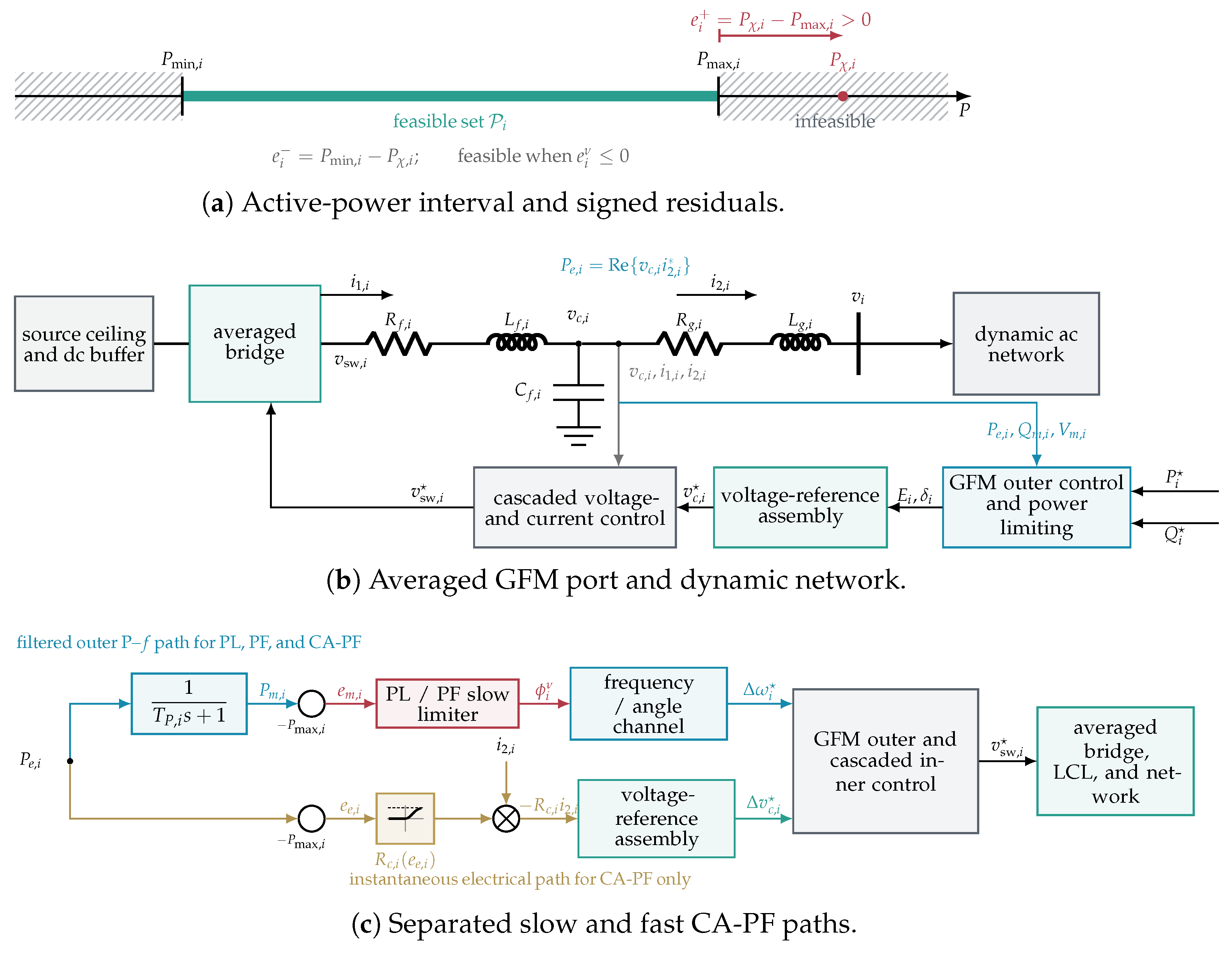
Figure 1 consolidates the constraint set, the averaged converter–network interface, and the two limiter actuation locations used throughout the formulation.

2.3. Active Branches and Local-Model Preservation

For architecture $c\in \{\mathrm{PL},\mathrm{PF},\mathrm{CA}\text{-}\mathrm{PF}\}$, define the equilibrium active set

$${\mathcal{A}}_c^{\nu }=\{i\mid {\overline{\varphi }}_{c,i}^{\nu }>0\}.$$

(10)

At a binding constraint with a positive multiplier, ${\overline{e}}_i^{\nu }=0$ and ${\overline{\lambda }}_i^{\nu }={\overline{\lambda }}_i^{s,\nu }>0$. The PF positive-part argument is then strictly positive, whereas the PL proportional term lies at its kink. Consequently, a fixed PF active branch has an ordinary Jacobian, while PL requires a generalized slope at the kink; Section 4.2 makes this relation explicit.

Let $F_{\mathrm{PF}}$ denote the full-order PF vector field on a declared active branch and let $\Delta F$ be a proposed augmentation. The sufficient local construction used here is

$$\Delta F\left(\overline{x}\right)=0,D\Delta F\left(\overline{x}\right)=0.$$

(11)

It separates three design requirements. The augmentation must preserve the constrained equilibrium, preserve the PF active-branch linearization used by the stability screen, and still produce a nonzero finite-amplitude response on the electrical time scale. Conditions (11) do not themselves guarantee nonlinear performance; they make the local stability claim auditable while the nonlinear case studies determine the useful finite-amplitude range.

3. Full-Order GFM-Network Model

3.1. General GFM-Network Interconnection

Consider a connected AC network with n GFM converters. Converter i has dynamic state $x_i\in {\mathbb{R}}^{n_i}$, terminal voltage $v_i\in {\mathbb{R}}^2$, injected current $i_i\in {\mathbb{R}}^2$, and parameters ${\theta }_i$. The network contributes dynamic branch, shunt, load, and optional algebraic states $x_N$. A broad class of averaged models can be written as

$$\begin{array}{cccc}\hfill E_i{\dot{x}}_i& =f_i(x_i,v_i,u_i;{\theta }_i),\hspace{1em}\hspace{1em}\hspace{1em}\hspace{1em}\hspace{1em}\hfill & \hfill i_i& =h_i(x_i,v_i;{\theta }_i),\hfill \end{array}$$

(12a)

$$\begin{array}{cccc}\hfill E_N{\dot{x}}_N& =f_N(x_N,i_1,\dots ,i_n,d;{\theta }_N),\hspace{1em}\hspace{1em}\hspace{1em}\hfill & \hfill v& =h_N(x_N,i,d;{\theta }_N),\hfill \end{array}$$

(12b)

where d collects load and reference disturbances. Singular $E_i$ or $E_N$ accommodates an index-one DAE; nonsingular matrices give an ODE. With stacked state $x=\mathrm{col}(x_N,x_1,\dots ,x_n)$ and $E=\mathrm{blkdiag}(E_N,E_1,\dots ,E_n)$, controller architecture $c\in \{\mathrm{PL},\mathrm{PF},\mathrm{CA}\text{-}\mathrm{PF}\}$ gives

$$E\dot{x}=F_c(x,d;\mu ,\theta ).$$

(13)

The scalar $\mu \ge 1$ is the convergence-rate multiplier defined in Section 4.5. The symbol s is reserved for the Laplace variable in transfer-function expressions. No bus count, topology, converter count, or benchmark has entered (13).

Assumption 1 (Local model regularity). 

On each declared topology and active region, the smooth converter and network maps are continuously differentiable. If E is singular, local coordinates $x=(y,z)$ put (13) into the semi-explicit index-one form

$$\dot{y}=f_c(y,z,d),0=g_c(y,z,d),$$

(14)

with $D_z{g}_c$ nonsingular in a neighborhood of the consistent operating point. Exogenous schedules are piecewise continuous, and every denominator introduced by a controller filter or activation map is strictly positive.

Assumption 1 is automatic for the dynamic RLC validation model because all bus capacitances and branch and load inductances are positive, making E nonsingular. Its network vector field is therefore an explicit ODE. It is nevertheless nonlinear and piecewise smooth because active and reactive powers are bilinear in voltage and current, the common frame speed is state-dependent, and positive-part, projection, and saturation maps enter the feedback. The descriptor notation retains applicability to index-one network realizations with algebraic buses without incorrectly classifying the validation model itself as a DAE.

3.2. Outer Command and Measurement

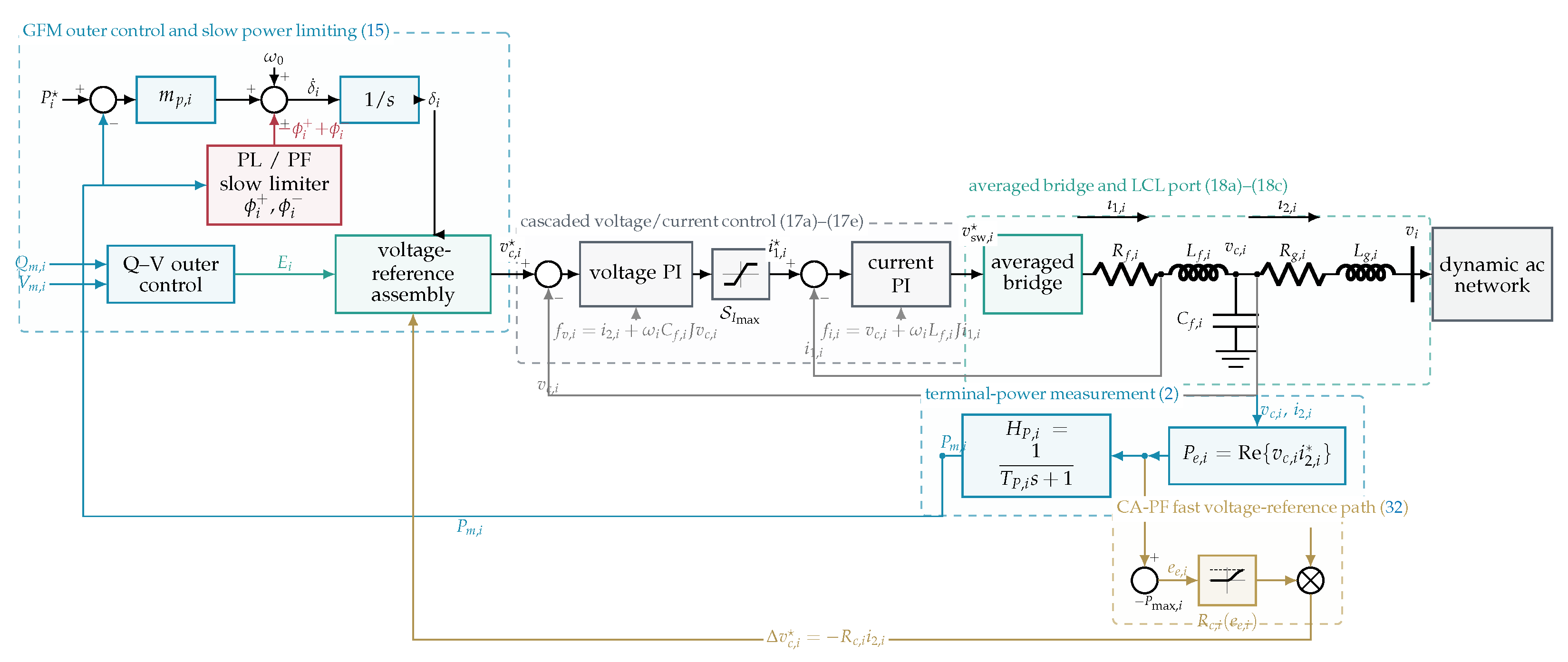
Figure 2 summarizes the converter signal flow, including the filtered slow limiter and the instantaneous CA-PF voltage-reference path. With $P_{e,i}$ and $P_{m,i}$ defined by (2), the power-limited frequency command is

$${\omega }_i^{★}={\omega }_0+m_{p,i}(P_i^{★}-P_{m,i})-{\varphi }_i^{+}+{\varphi }_i^{-},$$

(15)

with angle state ${\dot{\delta }}_i={\omega }_i^{★}-{\omega }_{\mathrm{ref}}$. The upper correction ${\varphi }_i^{+}$ slows a converter above $P_{\max ,i}$; the lower correction ${\varphi }_i^{-}$ speeds it below $P_{\min ,i}$. Voltage/reactive outer loops, current-reference limiting, inner voltage/current PI control, the averaged bridge, and the LCL dynamics are contained in $f_i$ rather than omitted from (12a).

This separation matters because the limiter acts through the angle/frequency channel, while its filtered power signal is produced by the inner controls, plant, and measurement state. Thus, a limiter gain can move an eigenpair containing angle, electrical, measurement, and network-current states even when the reduced active-power equilibrium is unchanged.

3.3. Equation-Level Converter Realization

A detailed converter state can be partitioned as $x_i=\mathrm{col}(x_i^{\mathrm{out}},x_i^{\lim },x_i^v,x_i^i,x_i^{\mathrm{LCL}},x_i^{\mathrm{damp}})$. These groups contain the outer control and measurements, power-limiter states, voltage- and current-controller integrators, electrical-filter states, and damping-filter states. The partition is descriptive; models with additional DC-side or measurement states remain covered by (12a). In the validation realization, the Q–V outer control, filtered $P/Q/V$ measurements, and current-limiter logic follow the REGFM_A1 structure [16]; only the active-power overload loop is replaced by PL, PF, or CA-PF.

Let $J=\left[\begin{array}{cc}0& -1\\ 1& 0\end{array}\right]$ and let ${\mathcal{S}}_{I_{\max }}$ denote circular, phase-preserving current-reference saturation,

$${\mathcal{S}}_{I_{\max }}\left(z\right)=\left\{\begin{array}{cc}0,\hfill & z=0,\hfill \\ z\min \left\{1,I_{\max }/{\parallel z\parallel }_2\right\},\hfill & z\ne 0.\hfill \end{array}\right.$$

(16)

The cascaded voltage/current realization follows [29].

$$\begin{array}{cc}\hfill e_{v,i}& =v_{c,i}^{★}-v_{c,i},\hfill \end{array}$$

(17a)

$$\begin{array}{cc}\hfill \hspace{1em}\hspace{1em}\hspace{1em}\hspace{1em}\hspace{1em}\hspace{1em}\hspace{1em} z_{v,i}& =K_{Pv,i}{e}_{v,i}+{\xi }_{v,i}+i_{2,i}+{\omega }_i{C}_{f,i}J{v}_{c,i},\hfill \end{array}$$

(17b)

$$\begin{array}{cc}\hfill \hspace{1em}\hspace{1em}\hspace{1em}\hspace{1em}\hspace{1em}\hspace{1em}\hspace{1em}\hspace{1em}\hspace{1em}\hspace{1em} i_{1,i}^{★}& ={\mathcal{S}}_{I_{\max ,i}}\left(z_{v,i}\right),{\dot{\xi }}_{v,i}=K_{Iv,i}{e}_{v,i}+{\displaystyle \frac{i_{1,i}^{★}-z_{v,i}}{T_{\mathrm{aw},i}}},\hfill \end{array}$$

(17c)

$$\begin{array}{cc}\hfill \hspace{1em}\hspace{1em}\hspace{1em}\hspace{1em}\hspace{1em}\hspace{1em} e_{i,i}& =i_{1,i}^{★}-i_{1,i},{\dot{\xi }}_{i,i}=K_{Ii,i}{e}_{i,i},\hfill \end{array}$$

(17d)

$$\begin{array}{cc}\hfill \hspace{1em}\hspace{1em}\hspace{1em}\hspace{1em}\hspace{1em}\hspace{1em}\hspace{1em}\hspace{1em}{v}_{\mathrm{sw},i}^{★}& =K_{Pi,i}{e}_{i,i}+{\xi }_{i,i}+v_{c,i}+{\omega }_i{L}_{f,i}J{i}_{1,i},\hfill \end{array}$$

(17e)

where $T_{\mathrm{aw},i}=5{\tau }_i$. The current-reference limiter remains inactive in the reported cases, so the anti-windup term does not affect the comparisons. One corresponding averaged LCL plant is

$$\begin{array}{cc}\hfill \hspace{1em}\hspace{1em}\hspace{1em}\hspace{1em}{L}_{f,i}{\dot{i}}_{1,i}& =v_{\mathrm{sw},i}-v_{c,i}-R_{f,i}{i}_{1,i}-{\omega }_i{L}_{f,i}J{i}_{1,i},\hfill \end{array}$$

(18a)

$$\begin{array}{cc}\hfill C_{f,i}{\dot{v}}_{c,i}& =i_{1,i}-i_{2,i}-{\omega }_i{C}_{f,i}J{v}_{c,i},\hfill \end{array}$$

(18b)

$$\begin{array}{cc}\hfill \hspace{1em}\hspace{1em}\hspace{1em}{L}_{g,i}{\dot{i}}_{2,i}& =v_{c,i}-v_i-R_{g,i}{i}_{2,i}-{\omega }_i{L}_{g,i}J{i}_{2,i}.\hfill \end{array}$$

(18c)

Sign changes induced by a different $dq$ convention do not alter the formulation. What matters here is that $P_{e,i}$ is generated by (17a)–(17e) and (18a)–(18c), $P_{m,i}$ adds a measurement state, and the PL/PF output changes ${\omega }_i^{★}$ upstream rather than the voltage reference.

The fixed common virtual-resistance and transient-damping channels follow the high-pass disturbance-rejection structure of [30], with washout currents

$${\tilde{i}}_{R,i}=\frac{{\tau }_{R,i}s}{{\tau }_{R,i}s+1}{i}_{2,i},{\tilde{i}}_{D,i}=\frac{{\tau }_{D,i}s}{{\tau }_{D,i}s+1}{i}_{2,i},$$

(19)

entering the voltage command as

$$\begin{array}{cc}\hfill \hspace{1em}{v}_{c,i}^{★d}& =E_i+K_{D,i}{\tilde{i}}_{D,i}^q-K_{R,i}{\tilde{i}}_{R,i}^d,\hfill \end{array}$$

(20a)

$$\begin{array}{cc}\hfill v_{c,i}^{★q}& =-K_{D,i}{\tilde{i}}_{D,i}^d-K_{R,i}{\tilde{i}}_{R,i}^q.\hfill \end{array}$$

(20b)

Both washout outputs vanish at equilibrium, but their states and gains alter the full-order spectrum; they therefore remain in $x_i^{\mathrm{damp}}$ during the stability screen. These channels are part of the common converter implementation, are identical for PL, PF, and CA-PF, and are not included in the proposed fast path.

4. Power-Limiting Architectures

4.1. Why the First Peak Survives Outer-Loop Retuning

Proposition 2 (No instantaneous outer-loop correction). 

Suppose an electrical disturbance begins at $t_0$ while the upper limiter is inactive, and suppose the disturbance does not reset the filter or multiplier states. Then, the PL and PF frequency-channel corrections have zero jump at $t_0$, independently of their finite gains.

Proof. 

The dynamic states are continuous, so (2) and either multiplier realization give

$$\delta \left(t_0^{+}\right)=\delta \left(t_0^{-}\right),\lambda \left(t_0^{+}\right)=\lambda \left(t_0^{-}\right),$$

(21)

and $P_m\left(t_0^{+}\right)=P_m\left(t_0^{-}\right)$. Hence,

$${\varphi }_{\mathrm{PL}}\left(t_0^{+}\right)-{\varphi }_{\mathrm{PL}}\left(t_0^{-}\right)={\varphi }_{\mathrm{PF}}\left(t_0^{+}\right)-{\varphi }_{\mathrm{PF}}\left(t_0^{-}\right)=0,$$

(22)

because $P_m\left(t_0^{+}\right)=P_m\left(t_0^{-}\right)$ and the limiter was inactive immediately before the event.    □

Thus, outer-loop retuning cannot produce an instantaneous correction in the studied realization. The proposed second path is driven by $P_e$ and acts directly at the voltage-reference location. Increasing $k_P$ or $k_I$ can accelerate the correction after $P_m$ departs from its pre-disturbance value. However, continuity of $P_m$ and the multiplier state prevents either gain from modifying the correction at disturbance onset.

4.2. Local PL/PF Slope Relation

Proposition 3 (Active-branch endpoint relation). 

Consider a binding constraint with equilibrium ${\overline{e}}_i^{\nu }=0$ and strictly positive multiplier ${\overline{\lambda }}_i^{\nu }={\overline{\lambda }}_i^{s,\nu }>0$. The PF branch is differentiable with

$$D{\varphi }_{\mathrm{PF},i}^{\nu }=k_{P,i}^{\nu }D{e}_i^{\nu }+D{\lambda }_i^{s,\nu },D{\dot{\lambda }}_i^{s,\nu }=k_{I,i}^{\nu }D{e}_i^{\nu },$$

(23)

while the PL Clarke generalized derivative [31] is

$$D{\varphi }_{\mathrm{PL},i}^{\nu }={\sigma }_i^{\nu }{k}_{P,i}^{\nu }D{e}_i^{\nu }+D{\lambda }_i^{\nu },D{\dot{\lambda }}_i^{\nu }=k_{I,i}^{\nu }D{e}_i^{\nu },$$

(24)

with ${\sigma }_i^{\nu }\in [0,1]$. Consequently, the physical PF active-branch Jacobian equals the ${\sigma }_i^{\nu }=1$ endpoint of the PL generalized-Jacobian family; inactive PF multiplier states contribute decoupled poles $-1/{\rho }_i^{\nu }$.

Proof. 

For PF, the argument of (9a) equals the strictly positive equilibrium multiplier, so the positive-part derivative is one; substitution in (9b) gives $D\dot{\lambda }=(1/\rho )k_{P}De=k_{I}De$. For PL, $\overline{\lambda }>0$ makes the tangent-cone dynamics locally unconstrained, but $k_P\overline{e}=0$ sits exactly at the positive-part kink, whose Clarke derivative is $\sigma \in [0,1]$. An inactive PF state has $\varphi =0$ locally, hence ${\dot{\lambda }}^s=-{\lambda }^s/\rho$ without an output path.    □

Proposition 3 clarifies the local relationship between the two baseline controllers. The PF active branch equals the unit-slope endpoint of the PL generalized-Jacobian family, while PL also retains the remaining generalized slopes. Consequently, any gain selection must be verified for the architecture to which it is applied.

Nearly coincident PL and PF overload traces at matched gains, as observed in the case studies, do not imply identical nonsmooth dynamics. PL retains the full generalized-slope interval at the projection boundary, so its local stability screen remains architecture-specific.

4.3. Constraint-Activated Projection-Free Control

The proposed controller augments the upper PF branch; the lower branch retains (9a) and (9b). In the notation of Section 2.1, define

$$e_{\chi ,i}:=e_i^{+}=P_{\chi ,i}-P_{\max ,i},e_{e,i}=P_{e,i}-P_{\max ,i}.$$

(25)

Here, $P_{\chi ,i}=P_{m,i}$ in the filtered detailed realization; the separate symbol only identifies the signal entering the slow limiter. The slow-path shaping map,

$${\psi }_{{\gamma }_i,{ϵ}_i}\left(e\right)=e+{\gamma }_i{\displaystyle \frac{{\left[e\right]}_{+}^2}{{ϵ}_i+{\left[e\right]}_{+}}},{\gamma }_i\ge 0,{ϵ}_i>0,$$

(26)

strengthens the multiplier for finite positive violation while keeping $\psi \left(0\right)=0$, ${\psi }^{\prime }\left(0\right)=1$. The shaped projection-free multiplier is

$$\begin{array}{cc}\hfill {\varphi }_{\mathrm{CA}\text{-}\mathrm{PF},i}^{+}& ={\left[k_{P,i}^{+}{\psi }_{{\gamma }_i,{ϵ}_i}\left(e_{\chi ,i}\right)+{\lambda }_i^{s,+}\right]}_{+},\hfill \end{array}$$

(27a)

$$\begin{array}{cc}\hfill {\dot{\lambda }}_i^{s,+}& ={\rho }_i^{-1}({\varphi }_{\mathrm{CA}\text{-}\mathrm{PF},i}^{+}-{\lambda }_i^{s,+}).\hfill \end{array}$$

(27b)

The fast path uses the bounded activation

$$R_{c,i}\left(e_{e,i}\right)={\overline{R}}_{c,i}{\displaystyle \frac{{\left[e_{e,i}\right]}_{+}^2}{{ϵ}_{R,i}^2+{\left[e_{e,i}\right]}_{+}^2}},0\le R_{c,i}\le {\overline{R}}_{c,i},$$

(28)

Lemma 1 (Regularity and order at the constraint boundary). 

For $\gamma \ge 0$, $ϵ>0$, ${\overline{R}}_c\ge 0$, and ${ϵ}_R>0$, the functions ${\psi }_{\gamma ,ϵ}$ and $R_c$ are continuously differentiable and locally Lipschitz on $\mathbb{R}$. Their derivatives are

$$\begin{array}{cc}\hfill {\psi }_{\gamma ,ϵ}^{\prime }\left(e\right)& =\left\{\begin{array}{cc}1,\hfill & e\le 0,\hfill \\ 1+\gamma {\displaystyle \frac{e(2ϵ+e)}{{(ϵ+e)}^2}},\hfill & e>0,\hfill \end{array}\right.\hfill \end{array}$$

(29a)

$$\begin{array}{cc}\hfill R_c^{\prime }\left(e\right)& =\left\{\begin{array}{cc}0,\hfill & e\le 0,\hfill \\ {\displaystyle \frac{2{\overline{R}}_c{ϵ}_R^{2}e}{{({ϵ}_R^2+e^2)}^2}},\hfill & e>0.\hfill \end{array}\right.\hfill \end{array}$$

(29b)

Moreover,

$$0\le R_c\left(e\right)\le {\overline{R}}_c,0\le {\psi }_{\gamma ,ϵ}\left(e\right)-e\le \gamma {\left[e\right]}_{+},$$

(30)

and, as $e\to 0$,

$${\psi }_{\gamma ,ϵ}\left(e\right)-e=O\left({\left[e\right]}_{+}^2\right),R_c\left(e\right)=O\left({\left[e\right]}_{+}^2\right).$$

(31)

Proof. 

For $e\le 0$, the positive part vanishes, so $\psi \left(e\right)=e$ and $R_c\left(e\right)=0$. For $e>0$, ordinary differentiation gives (29a) and (29b). Their right limits at zero are 1 and 0, respectively, which equal the left derivatives. The bounds follow from $0\le e^2/(ϵ+e)\le e$ and $0\le e^2/({ϵ}_R^2+e^2)\le 1$ for $e>0$. Finally, division by the strictly positive denominators gives the second-order estimates in (31).    □

Proposition 4 (Local well-posedness of the PF and CA-PF dynamics). 

Under Assumption 1, every consistent PF or CA-PF initial condition admits a unique local solution on each interval with fixed topology and continuous exogenous input. If E is nonsingular, this solution is generated directly by a locally Lipschitz ODE. If E is singular, the index-one algebraic variables can be eliminated locally, yielding an equivalent locally Lipschitz ODE in the differential variables.

Proof. 

The positive-part and saturation maps are Lipschitz, while Lemma 1 makes the added CA-PF maps continuously differentiable. Composition with the smooth plant and controller maps therefore produces a locally Lipschitz vector field when E is nonsingular, so the standard local existence and uniqueness result applies [32]. In the index-one case, nonsingularity of $D_z{g}_c$ in (14) gives a local function $z=\zeta (y,d)$ by the implicit-function theorem. Substitution produces $\dot{y}=f_c(y,\zeta (y,d),d)$, to which the same ODE argument applies [33]. Piecewise-continuous schedules are handled by concatenating the unique solutions at their declared event times.    □

Proposition 4 guarantees the existence and uniqueness of the local controller-network trajectory for each consistent initial condition on a fixed topology and continuous-input interval. Subsequent limiter or topology transitions require the corresponding branch assumptions to be re-established.

The fast path modifies the capacitor-voltage reference according to

$$v_{c,i}^{★,\mathrm{CA}\text{-}\mathrm{PF}}=v_{c,i}^{★,\mathrm{PF}}-R_{c,i}{i}_{2,i}.$$

(32)

Substituting (20a) and (20b) gives the following two-axis form.

$$\begin{array}{cc}\hfill \hspace{1em} v_{c,i}^{★d,\mathrm{CA}\text{-}\mathrm{PF}}& =E_i+K_{D,i}{\tilde{i}}_{D,i}^q-K_{R,i}{\tilde{i}}_{R,i}^d-R_{c,i}{i}_{2,i}^d,\hfill \end{array}$$

(33a)

$$\begin{array}{cc}\hfill v_{c,i}^{★q,\mathrm{CA}\text{-}\mathrm{PF}}& =-K_{D,i}{\tilde{i}}_{D,i}^d-K_{R,i}{\tilde{i}}_{R,i}^q-R_{c,i}{i}_{2,i}^q,\hfill \end{array}$$

(33b)

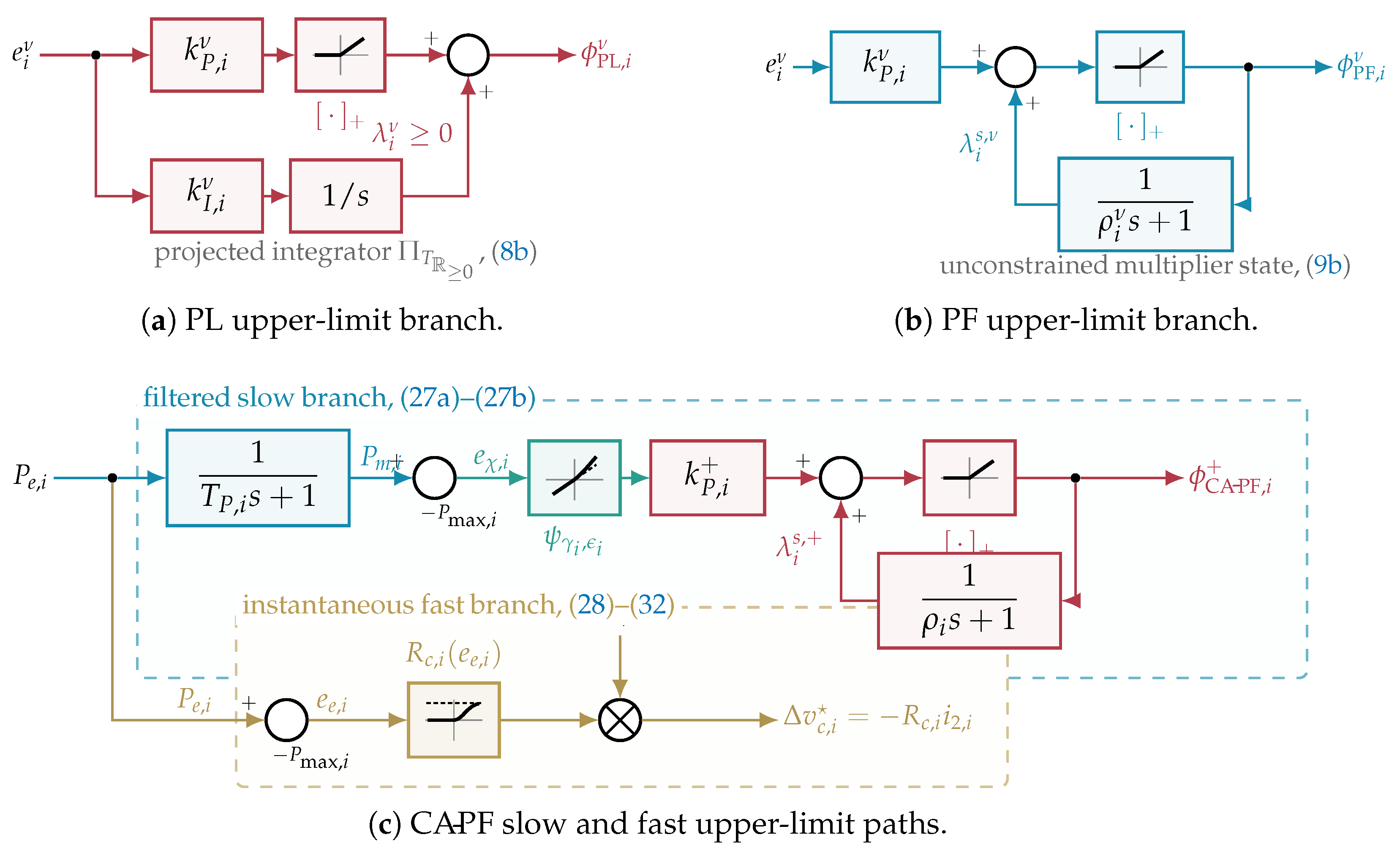
i.e., a same-axis resistive drop on both d and q, not a d-axis-only correction. Because $R_{c,i}\le {\overline{R}}_{c,i}$, $\parallel R_{c,i}{i}_{2,i}\parallel \le {\overline{R}}_{c,i}\parallel i_{2,i}\parallel$; $I_{\max ,i}$ limits $i_{1,i}^{★}$, not $i_{2,i}$. In the central case, ${\max }_t\parallel i_{2,2}\parallel \approx 0.61$ p.u. and the commanded voltage-reference depression $\parallel R_{c,2}{i}_{2,2}\parallel$ peaks at approximately 0.012 p.u. (1.2% of nominal voltage). Together with (15), these relations complete the proposed controller. Thus, CA-PF combines a shaped PF slow path with a bounded fast resistance path. Figure 3 compares this structure with the PL and PF upper-limit branches. The word “resistance” in (28) describes the implemented voltage drop; it is not the fixed washout-based background channel in (20a) and (20b). Existing adaptive-resistance methods target current or postfault oscillations [25,26]; here, $R_c$ is triggered directly by source active-power exceedance and coordinated with the PF multiplier.

Equation (28) uses terminal power measured before the slower outer $P_m$ filter, with synchronized voltage and current acquisition and practical anti-alias conditioning. Let the implemented signal be ${\widehat{P}}_e=P_e+n$ with $\left|n\right|\le {\eta }_P$. Whenever the true residual is nonpositive, ${\left[{\widehat{P}}_e-P_{\max }\right]}_{+}\le {\eta }_P$, and therefore

$$0\le R_c({\widehat{P}}_e-P_{\max })\le {\overline{R}}_c{\displaystyle \frac{{\eta }_P^2}{{ϵ}_R^2+{\eta }_P^2}}.$$

(34)

If the pre-event power margin exceeds ${\eta }_P$, false activation is excluded. Otherwise, (34) quantifies the worst boundary activation and shows why ${ϵ}_R$ should exceed the measurement-noise scale. Practical implementation should use synchronized voltage and current samples with anti-alias filtering whose delay is short relative to the electrical peak. Any additional measurement-filter or computation-delay state must be included in the full-order screen and finite-disturbance tests.

4.4. Preservation of the Equilibrium and Local Model

Proposition 5 (Preservation of the equilibrium and active-branch Jacobian). 

Consider a strictly active upper-limit PF equilibrium with ${\overline{P}}_e={\overline{P}}_m=P_{\max }$ and ${\overline{\lambda }}^{s,+}>0$. For any finite $\gamma \ge 0$, $ϵ>0$, ${\overline{R}}_c\ge 0$, ${ϵ}_R>0$, CA-PF has the same equilibrium and active-branch Jacobian as PF.

Proof. 

At the binding equilibrium, ${\overline{P}}_e={\overline{P}}_m=P_{\max }$, so the activation residual is $e=0$ and

$$\psi \left(0\right)=0,{\psi }^{\prime }\left(0\right)=1,R_c\left(0\right)=0,R_c^{\prime }\left(0\right)=0,$$

(35)

Consequently, (27a) and (27b) reduce to the PF equilibrium and differential in (23), and (32) contributes neither an equilibrium offset nor a first-order perturbation. Every remaining converter and network equation is unchanged.    □

At a binding equilibrium, Proposition 5 establishes identical steady voltage and frequency corrections and identical first-order responses for PF and CA-PF. The proposed paths become active only for finite positive violations, which isolates their effect to the finite-amplitude overload trajectory.

Corollary 1 (Preservation of local eigenvalues). 

Under Proposition 5, PF and CA-PF have the same linearized model on the strict active branch. Their finite eigenvalues, including algebraic multiplicities, therefore coincide. Consequently, the real part of the rightmost finite eigenvalue and the resulting local small-signal stability conclusion are identical.

Proof. 

The matrix E is unchanged, and Proposition 5 gives $A_{\mathrm{CA}\text{-}\mathrm{PF}}=A_{\mathrm{PF}}$. Therefore, both linearized models yield the same generalized eigenvalue equation and hence the same finite eigenvalues.    □

Proposition 5 and Corollary 1 are deliberately local. They preserve the screened PF small-signal model while allowing different finite-amplitude trajectories, but they prove neither a region of attraction nor immunity to current limiting.

For a large-signal disturbance, the local result is used as a non-degradation condition rather than as a global certificate. It verifies that the proposed paths do not introduce a new first-order mode at the constrained equilibrium. The response away from that equilibrium is then evaluated with the nonlinear full-order model, including finite load steps, changing active sets, parameter corners, and current-limit monitoring. This division is intentional. The propositions establish the local property that can be proved from the boundary construction, whereas the simulations supply finite-amplitude evidence within the declared test set.

4.5. Convergence-Rate Gain Scaling

The scaling studied in [18] reads, in the implemented variables,

$$k_{I,i}\left(\mu \right)=\mu k_{I,i0},k_{P,i}\left(\mu \right)=\sqrt{\mu }{k}_{P,i0},{\rho }_i\left(\mu \right)={\rho }_{i0}/\sqrt{\mu },$$

(36)

for $\mu \ge 1$. It preserves the constrained fixed point (the gains multiply zero equilibrium errors) but changes transient time scales and the full-order Jacobian. The logical separation enforced in this paper is

$$\underset{\mathrm{reduced}\text{-}\mathrm{model}\mathrm{result}}{\underbrace{{\beta }_{\mathrm{red}}\left(\mu \right)\mathrm{improves}}}\nRightarrow \underset{\mathrm{detailed}\mathrm{closed}\text{-}\mathrm{loop}\mathrm{stability}}{\underbrace{{\alpha }_{\mathrm{full}}\left(\mu \right)<0}}.$$

(37)

This paper tests and enforces the right-hand condition; it does not re-derive the left-hand theorem.

Increasing $\mu$ raises $k_I$, raises $k_P$ by its square root, and shortens $\rho$. It can accelerate the intended slow limiter while also changing its interaction with measurement, electrical, and network states. It may increase the initial frequency excursion and sensitivity to imperfect power measurements, and it need not improve every active set monotonically. Hence, $\mu$ is stopped inside the verified full-order range and selected from a damping–excursion tradeoff rather than maximized.

5. Full-Order Stability-Constrained Design

5.1. Fixed-Branch Linearization and Screens

For scenario $q\in \mathcal{Q}$, let ${\overline{x}}_c\left(q\right)$ solve $F_c({\overline{x}}_c,0;\mu ,{\theta }_q)=0$ with declared active set $\mathcal{A}\left(q\right)$. On a smooth PF/CA-PF branch, or for a selected PL slope $\sigma$, linearization gives the generalized eigenvalue problem

$$\det \left(\lambda E_q-A_c(\mu ,q,\sigma )\right)=0,A_c={\left.\partial F_c/\partial x\right|}_{{\overline{x}}_c},$$

(38)

whose rightmost finite eigenvalue has real part

$${\alpha }_c(\mu ,q,\sigma )=\max \{\mathrm{Re}\left(\lambda \right)\mid \det (\lambda E_q-A_c)=0,\left|\lambda \right|<\infty \}.$$

(39)

For PL at a binding proportional kink, the generalized-slope screen is

$${\overline{\alpha }}_{\mathrm{PL}}(\mu ,q)=\underset{\sigma \in {[0,1]}^{\left|\mathcal{A}\right(q\left)\right|}}{\sup }{\alpha }_{\mathrm{PL}}(\mu ,q,\sigma ),$$

(40)

while ${\overline{\alpha }}_{\mathrm{PF}}$ uses the smooth active branch. Proposition 5 gives, at every strict binding equilibrium satisfying its assumptions,

$$A_{\mathrm{CA}\text{-}\mathrm{PF}}(\mu ,q)=A_{\mathrm{PF}}(\mu ,q),{\alpha }_{\mathrm{CA}\text{-}\mathrm{PF}}(\mu ,q)={\alpha }_{\mathrm{PF}}(\mu ,q).$$

(41)

A negative value of (40) is a local eigenvalue-based stability screen, not a common nonsmooth Lyapunov proof; pointwise quadratic or decentralized parametric certificates [21,32] would be stronger than the branchwise tests used here.

5.2. Architecture-Specific Stability Screen

For each scenario, define the largest fixed-branch stable-range limit

$${\mu }_{\mathrm{stab},c}\left(q\right)=\sup \left\{\overline{\mu }\ge 1|{\overline{\alpha }}_c(\mu ,q)<0\forall \mu \in [1,\overline{\mu }]\right\}.$$

(42)

Numerical continuation and refinement return a verified stable lower endpoint

$$1\le {\underline{\mu }}_c\left(q\right)\le {\mu }_{\mathrm{stab},c}\left(q\right),{\overline{\alpha }}_c(\mu ,q)<0\forall \mu \in [1,{\underline{\mu }}_c\left(q\right)].$$

Given requested multiplier ${\mu }_{\mathrm{req}}$ and design factor $0<\eta <1$, the implemented value is

$$\begin{array}{|c|}\hline {\mu }_{\mathrm{use},c}=\min \left\{{\mu }_{\mathrm{req}},\eta \underset{q\in \mathcal{Q}}{\inf }{\underline{\mu }}_c\left(q\right)\right\}.\\ \hline\end{array}$$

(43)

The scenario set may contain operating points, active sets, topologies, and parameter corners; it must be stated, since (43) has no meaning without it, and $\eta$ provides separation from a verified stable endpoint, not a probabilistic guarantee. For each scenario, the relevant equilibrium branch and verified stable range are identified before (43) is applied. The retained value is then checked by nonlinear disturbances. Within the declared fixed branches, the screen selects a slow-path multiplier for which the real part of the rightmost finite eigenvalue remains negative; by (41), CA-PF inherits the PF fixed-branch screen without claiming identical finite-amplitude trajectories.

5.3. Practical Parameter-Selection Algorithm

The parameter dependencies are organized in Algorithm 1. The sequence separates baseline stabilization, slow-path shaping, fast-path activation, and full-order acceptance.

Algorithm 1 Stability-Constrained CA-PF Parameter Selection

Stage 1:  Baseline design. The underlying GFM, inner loops, and baseline PF limiter are established first. The gains $k_P$, $k_I$, and $\rho =k_P/k_I$ follow the target reduced-model response and are retained only after the full-order fixed-branch screen. Stage 2:  Full-order scaling. Candidate values of μ follow (36) and remain below the architecture-specific ceiling in (43). The retained value is the smallest candidate that provides the required decay improvement within the prescribed frequency-excursion limit. Stage 3:  Slow-path shaping. The parameter ϵ defines the positive-violation scale at which the added slow action becomes appreciable. The parameter γ controls the finite-violation strength as the shaping slope increases from 1 at the boundary toward $1+\gamma$. A one-dimensional γ sweep quantifies the excess-energy and frequency-response tradeoff. Stage 4:  Fast-path activation. The knee ${ϵ}_R$ is placed above the characterized power-measurement noise and resolution, with $R_c\left({ϵ}_R\right)={\overline{R}}_c/2$. The ceiling ${\overline{R}}_c$ is constrained jointly by the overload target and the allowable voltage-reference depression. A conservative voltage budget is $${\overline{R}}_c\le {\displaystyle \frac{\Delta v_{\max }^{★}}{I_{2,\max }}},$$ (44) where $\Delta v_{\max }^{★}$ is the allowed command depression and $I_{2,\max }$ is a declared terminal-current bound. Stage 5:  Full-order acceptance. The selected tuple $(k_P,k_I,\rho ,\mu ,\gamma ,ϵ,{\overline{R}}_c,{ϵ}_R)$ is accepted only after verification across the declared operating points, active sets, parameter corners, measurement quality, current-limit margin, capacitor voltage, and reactive-power sharing. Among feasible candidates, the smallest ${\overline{R}}_c$ and γ satisfying the peak and exposure targets are retained.

6. Materials and Numerical Methods

6.1. Kron-Reduced Dynamic IEEE 9-Bus Model

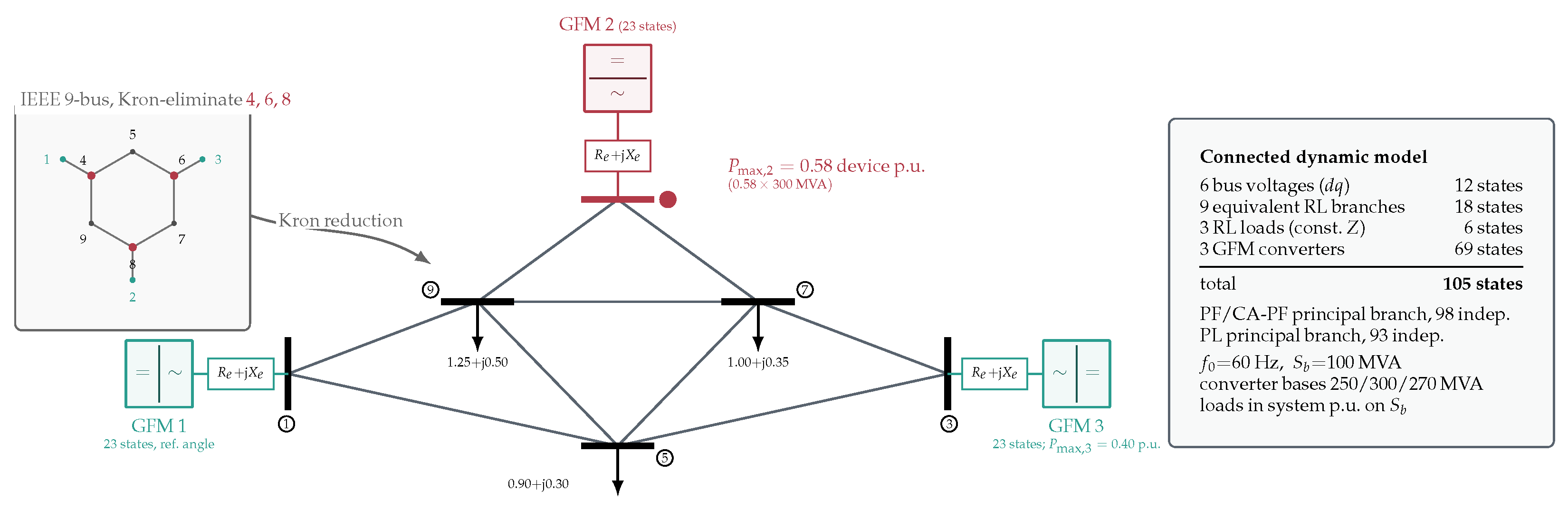
The general formulation is evaluated on a dynamic IEEE 9-bus environment used only as a validation network. The operating point follows the standard case9 solution [34]. Kron elimination of the passive zero-injection junction buses 4, 6, and 8 leaves the six-bus equivalent of Figure 4. It contains six dynamic bus voltages (12 states), nine equivalent RL branches (18), and three RL loads (6), which give 36 network states. Three 23-state converters replace the synchronous units at buses 1–3 and connect through their $R_e+\mathrm{j}{X}_e$ coupling branches, producing a 105-state nonlinear, piecewise-smooth ODE at $f_0=60$ Hz. Unit 1 defines the common moving $dq$ reference frame; its absolute angle is anchored only for equilibrium and eigenvalue calculations to remove the rotational coordinate.

The common converter model retains the REGFM_A1 P–f droop, Q–V outer control, filtered $P/Q/V$ measurements, and current-reference limiter [16]. The inner control follows (17a)–(17e) and (18a)–(18c). PL, PF, or CA-PF replaces only the active-power overload loop. After removing the reference angle and the six inactive reactive-limit multipliers, the PF and CA-PF principal branches retain $105-1-6=98$ independent states; PL additionally removes its five inactive projected multipliers, retaining 93. Inactive PF multipliers are kept because they are ordinary decaying states with poles $-1/\rho$; the endpoint comparisons of Section 8 therefore match physical dominant eigenpairs rather than requiring equal matrix dimensions.

The inner current gains follow $K_{Pi}=(L_f/{\omega }_0)/{\tau }_i$ and $K_{Ii}=R_f/{\tau }_i$;

Table 1. Case-study parameters (device p.u. unless noted).

Quantity	Value
Droop $m_p$, $m_q$; filters $T_P,T_Q,T_V$	0.01, 0.05; 10 ms
LCL $L_f,R_f,C_f$; coupling $R_e+\mathrm{j}{X}_e$	0.1, 0.01, 0.05; $\mathrm{j}$0.15
Outer Q–V PI $(K_{Pv}^{\mathrm{out}},K_{Iv}^{\mathrm{out}})$; $E_{\min },E_{\max }$	$(0,5.86)$; $(0,1.15)$
Reactive limiter $(Q_{\min },Q_{\max })$; $(k_{Pq},k_{Iq})$	$(-0.44,0.44)$; $(3,20)$
Inner voltage PI $(K_{Pv},K_{Iv})$; current feedforward ${\beta }_i$	$(1.6,600)$; 1
Inner current PI $(K_{Pi},K_{Ii})$; current loop ${\tau }_i$	$(1.061,40)$; 0.25 ms
Current limit $I_{\max }$ (circular)	2
System base; GFM bases [MVA]	100; $(250,300,270)$
Base limiter $(k_{P0},k_{I0},{\rho }_0)$	$(0.01,0.1,0.1)$
CA-PF $(\gamma ,ϵ,{\overline{R}}_c,{ϵ}_R)$	$(4,0.01,0.05,0.01)$
Common virtual resistance/transient damping $(K_R,K_D)$; $({\tau }_R,{\tau }_D)$	$(0.03,0.03)$; 4 ms
Baseline/selected CA-PF multiplier $\mu$	1/10
Stability-screen ceiling; smallest verified stable endpoint	86.4; 96.0
Central load event	$\times 1.2$, 1.5–3 s
GFM 2 source ceiling	0.58 (174 MW)
Multi-stage load event	$\times 1.2/\times 1.3$, reversed at 3.5/4.5 s
GFM 3 stage-2 source ceiling	0.4 (108 MW)
Source audit $H_{\mathrm{dc}}$; voltage floor	20 ms; 0.95 p.u.
Slow-path horizon; modal pulse	3 s; $+0.2\%$, 0.4–0.45 s

reports the resulting values to four significant digits.

The common channels (20a) and (20b) use $K_R=K_D=0.03$ and ${\tau }_R={\tau }_D=4$ ms for every controller. They are held fixed in the matched comparisons and are not counted as part of CA-PF. To check that the overload conclusion is not tied to one gain pair, the central PF and CA-PF tests were repeated for every combination $K_R,K_D\in \{0.02,0.03,0.04\}$. CA-PF retained a 53.9–55.6% peak reduction and approximately 53.4% violation-area reduction, without current-limiter activation.

Two additional converter-parameter corners vary $L_f$, $R_f$, and $C_f$ together by $-10\%$ and $+10\%$ while leaving all controller gains unchanged. A separate measurement-quality test adds a bounded, zero-mean power-measurement perturbation of 0.002 device p.u., equal to 0.6 MW on GFM 2, using 120 and 300 Hz components. The same perturbation enters the filtered-power measurement and the CA-PF fast signal. This averaged-model test represents bounded high-frequency measurement contamination, not semiconductor switching or an EMT validation.

6.2. Matched Overload Tests

All controllers start from the same nominal equilibrium. At $t=1.5$ s, every constant-impedance load is multiplied by the scenario stress factor; at $t=3$ s, loads are restored, and simulation continues to 3.5 s. GFM 2 is rated on a 300 MVA converter base and initially supplies 163 MW. Its upper limit is interpreted as the available source power, $P_{\max ,2}=0.58$ device p.u., or 174 MW, rather than the converter nameplate. The independent circular AC-current-reference limit remains 2 p.u. No CA-PF parameter changes between scenarios. All matched PL, PF, and CA-PF comparisons in Figure 5 use the baseline multiplier $\mu =1$; the selected value $\mu =10$ is evaluated only in the separate slow-path verification. The two primary violation metrics on the monitored unit are

$$\begin{array}{cc}\hfill V^{\mathrm{pk}}& ={\max }_t{\left[P_{e,2}\left(t\right)-P_{\max ,2}\right]}_{+},\hfill \\ \hfill J& ={\int }_{t_1}^{t_2}{\left[P_{e,2}\left(t\right)-P_{\max ,2}\right]}_{+}dt,\hfill \end{array}$$

(45)

alongside time above a 0.001 p.u. exceedance, peak $R_c$, and current-reference-limiter activation. On the 300 MVA base, $V^{\mathrm{pk}}$ in p.u. converts to megawatts by multiplication by 300, and J converts to megajoules by the same factor. The source-buffer audit applies (5) to each verified power trace at $H_{\mathrm{dc}}=20$ ms and at the 0.95 p.u. voltage floor. All controller comparisons retain the same filtered active-power measurement architecture.

6.3. Stable Slow-Path Verification

Slow-path scaling is verified separately from overload performance. Across the declared fixed active sets, the smallest numerically verified stable endpoint is ${\underline{\mu }}_{\mathrm{CA}\text{-}\mathrm{PF}}$$=96.0$. Applying (43) with $\eta =0.9$ gives a stable-screen ceiling of 86.4. The reported value $\mu =10$ is selected within that ceiling because it gives the most negative principal rightmost-eigenvalue real part in the sampled stable sweep. A $0.2\%$, 50 ms pulse and small modal perturbations compare it with the stable baseline $\mu =1$. For the nonlinear check, let $z\left(t\right)$ denote the corresponding modal coordinate. Its envelope is fitted as

$$\left|z\left(t\right)\right|\approx C\exp \left({\alpha }_{\mathrm{fit}}t\right),$$

where ${\alpha }_{\mathrm{fit}}$ is the time-domain fitted decay rate, not a second eigenvalue. Every accepted case is required to have a negative rightmost-eigenvalue real part and a negative time-domain fitted decay rate. Every nonlinear CA-PF result uses $\gamma =4$ and ${\overline{R}}_c=0.05$ p.u.

7. Results

7.1. Matched Response and Controller Mechanism

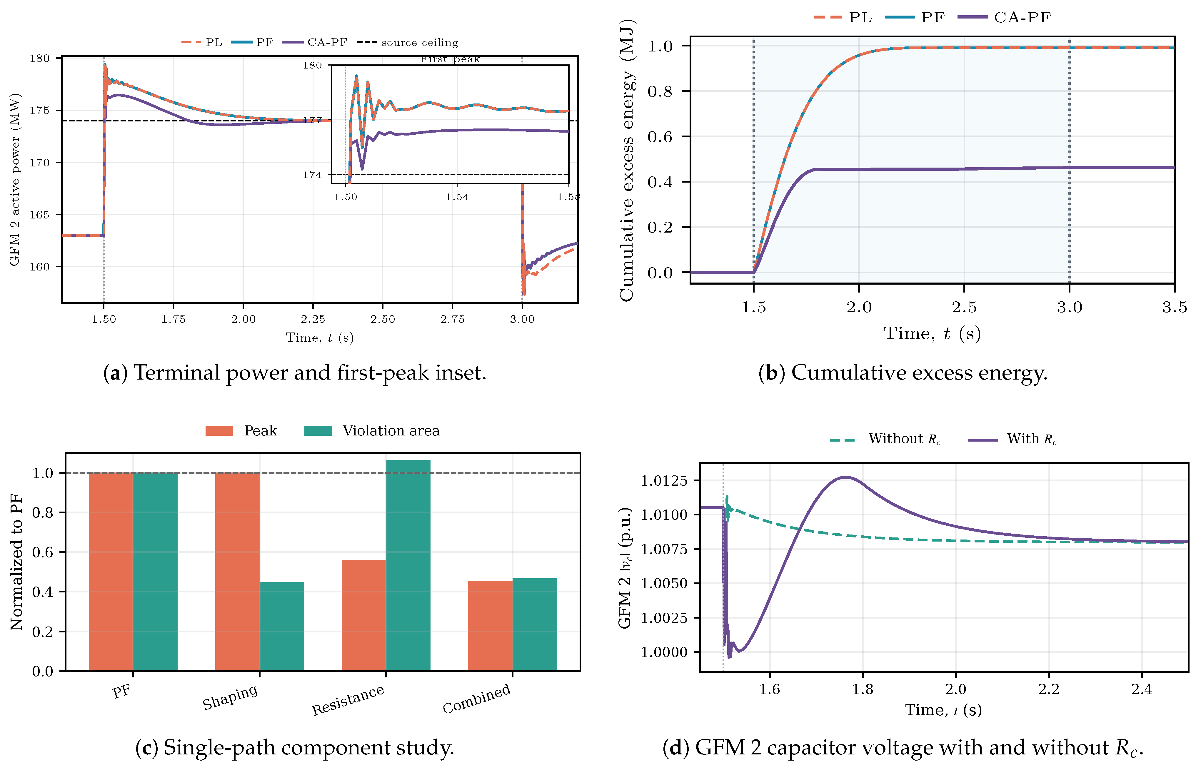
Figure 5a shows the central overload under the common filtered active-power measurement architecture. The main axes include load application and restoration, while the inset resolves the first peak. Base-gain PL and PF are visually coincident. Both exceed the 174-MW source ceiling by approximately 5.41 MW and accumulate approximately 0.991 MJ of excess energy. CA-PF reduces the peak exceedance to 2.45 MW and the excess energy to 0.462 MJ.

Because J is an accumulated exposure, Figure 5b shows how the two peak reductions translate into energy. The coincident PL/PF curves reach 0.991 MJ, whereas CA-PF levels off at 0.462 MJ. The single-path component study in Figure 5c shows that shaping cuts J by 55.2% without changing $V^{\mathrm{pk}}$, whereas resistance cuts the peak by 44.2% but raises J by 6.5%. Only the combined controller reduces both metrics by more than 50%.

Figure 5d isolates the voltage-side mechanism by comparing shaped CA-PF with and without $R_c$. The shaped slow path is identical in both traces. During the first transient, the commanded reference depression peaks at approximately 0.012 p.u., while the observed GFM 2 capacitor-voltage magnitude differs by at most 0.011 p.u. The latter is the closed-loop plant response, not the command norm. The voltage then returns to the no-resistance trajectory as the electrical transient decays. Thus, the added path produces a short voltage depression that suppresses the electrical power peak rather than a persistent voltage offset.

The same isolated comparison gives a maximum transient reactive-power difference of 0.0138 device p.u., or 4.13 MVAr on the 300 MVA base, and the two reactive-power trajectories return to the same final value. Thus, $R_c$ does perturb voltage magnitude and reactive-power sharing during activation, but the tested effect is bounded and temporary. Applications with tighter voltage or reactive-sharing requirements should reduce ${\overline{R}}_c$ through (44) and reassess the peak-reduction tradeoff. The central active-power and source-buffer metrics are summarized in

Table 2. Central active-power-limiting and source-buffer metrics.

Metric	PL	PF	CA-PF
Peak excess [MW]	5.41	5.41	2.45
Excess energy [MJ]	0.991	0.991	0.462
Time above 0.3 MW [s]	0.52	0.52	0.27
Min. $v_{\mathrm{dc}}$, $H_{\mathrm{dc}}=20$ ms [p.u.]	0.914	0.914	0.961
$H_{\mathrm{dc}}^{\min }$, 0.95 p.u. floor [ms]	33.9	33.9	15.8

.

7.2. Source-Side Consequence and Matched Comparison

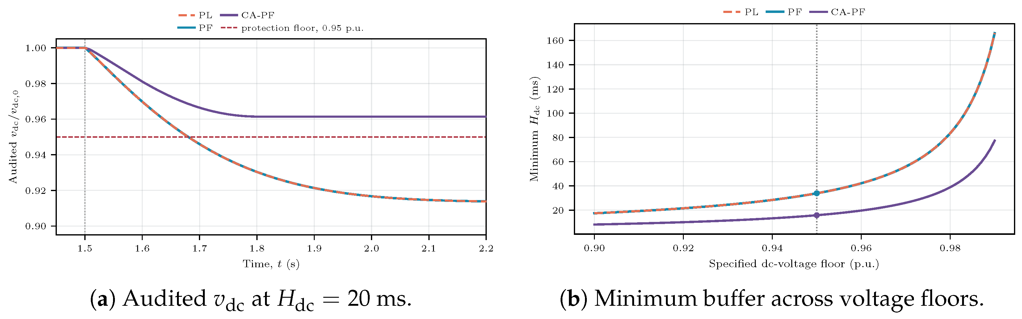
The source audit in Figure 6a makes the practical consequence explicit. With $H_{\mathrm{dc}}=20$ ms, PL and PF cross the 0.95 p.u. floor about 180 ms after the load step and reach approximately 0.914 p.u.; CA-PF remains at 0.961 p.u. At the same floor, Figure 6b gives minimum buffer constants of 33.9 ms for PL/PF and 15.8 ms for CA-PF. The current-reference limiter remains inactive in every realization.

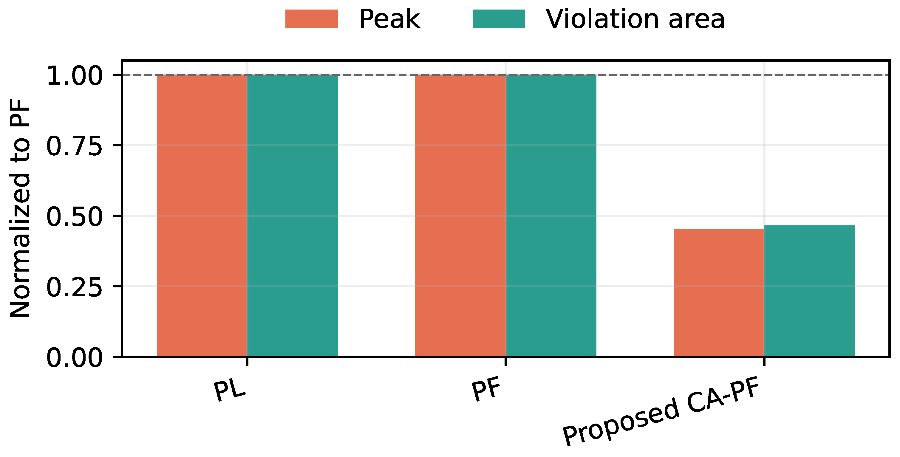
Figure 7 places the matched baseline PL and PF results beside the proposed CA-PF result, with both metrics normalized to PF. The coincident PL/PF bars confirm their matched behavior, whereas CA-PF reduces both the first peak and the violation area.

7.3. Resistance-Ceiling Selection

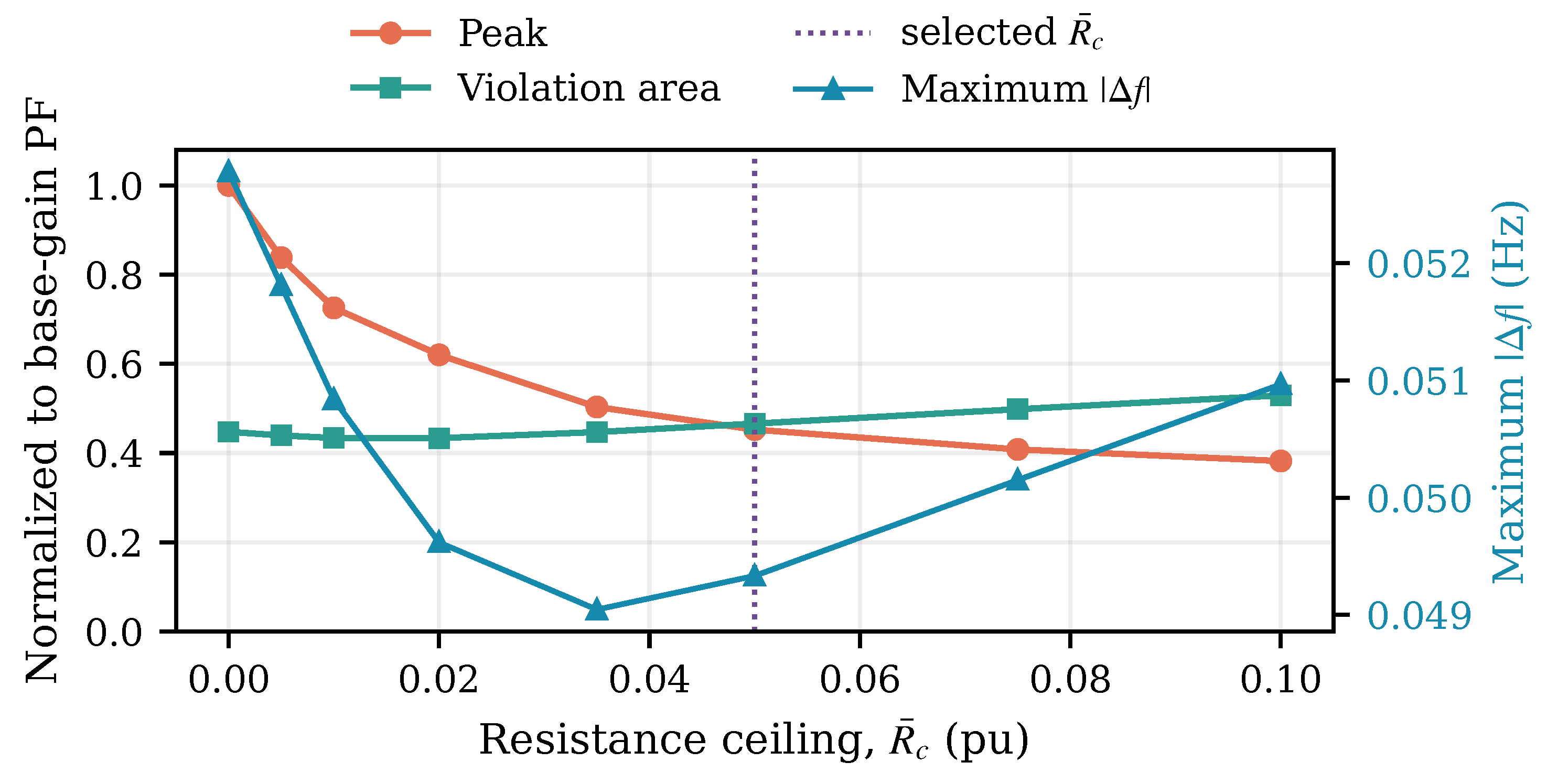
Proposition 5 already establishes that ${\overline{R}}_c$ cannot change the strict active-branch Jacobian because $R_c\left(0\right)=R_c^{\prime }\left(0\right)=0$. The resistance ceiling must therefore be selected from finite-amplitude performance rather than a root locus. Figure 8 shows that the peak falls monotonically, while violation area and frequency deviation form a design knee. The selected ${\overline{R}}_c=0.05$ p.u. is the first tested ceiling at which both peak and area lie below one half of base PF. This balanced threshold is not a claim of per-metric optimality. The current-reference limiter stays inactive throughout.

8. Robustness and CA-PF Slow-Path Stability

8.1. Ten-Scenario Robustness

Table 3. PL, PF, and proposed CA-PF across ten full-order scenarios.

	Peak Exceedance [MW]			CA-PF Reduction vs. PF [%]
Scenario	PL	PF	CA-PF	Peak	Excess Energy
Central	5.41	5.41	2.45	54.7	53.4
Moderate load	1.48	1.48	0.79	46.4	34.1
Severe load	9.23	9.23	4.53	51.0	59.2
Tight limit	11.41	11.41	6.99	38.7	62.2
Slow measurement	5.41	5.41	2.71	49.9	51.1
Weak network	5.98	5.98	2.67	55.4	50.9
Droop heterogeneity	5.41	5.41	2.52	53.4	47.5
LCL parameters $-10\%$	5.42	5.42	2.45	54.9	53.4
LCL parameters $+10\%$	5.40	5.40	2.45	54.7	53.5
Bounded measurement noise	5.41	5.41	2.82	47.8	52.0

reports every tested droop-controlled GFM scenario with unchanged CA-PF parameters on the same 300 MVA GFM 2 base. It now exposes both matched baselines rather than showing PF alone. PL and PF agree to the displayed peak precision in all cases, and their excess energies differ by less than 1%. Peak reduction relative to PF ranges from 38.7% to 55.4%, and excess-energy reduction ranges from 34.1% to 62.2%. The $\pm 10\%$ LCL corners retain approximately 54.7% peak reduction and 53.4% energy reduction. Under bounded measurement noise, the corresponding reductions are 47.8% and 52.0%, with no false pre-event activation because the operating margin exceeds the imposed noise bound. For a common voltage floor, (7) gives the same percentage reduction in required $H_{\mathrm{dc}}$. Every reduction remains positive, terminal-power exceedance returns to zero after load restoration, and the current-reference limiter remains inactive. These are deterministic sensitivity tests over the declared set, not a probabilistic robustness guarantee.

8.2. Sequential Multi-Source Constraint Activation

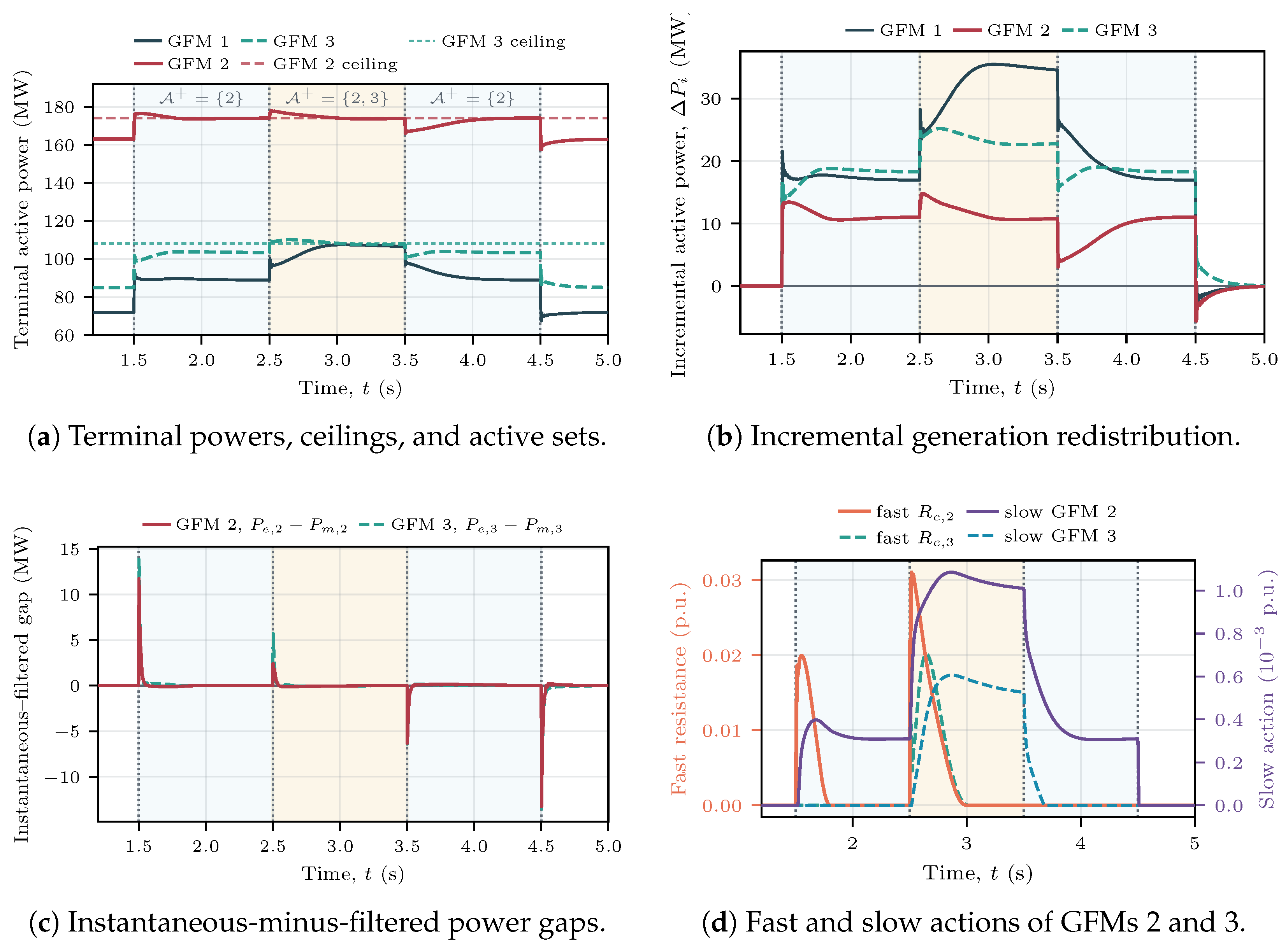
The preceding matched comparison establishes the benefit on one constrained unit. The CA-PF-only network trajectory is extended here to test sequential activation of two source ceilings without introducing a voltage or frequency disturbance. Starting from terminal powers of approximately 72, 163, and 85 MW, the balanced load multiplier changes from 1 to 1.2 at 1.5 s and to 1.3 at 2.5 s. These changes are reversed at 3.5 and 4.5 s. The declared ceilings are 174 MW for GFM 2 and 108 MW for GFM 3, giving initial headrooms of 11 and 23 MW.

Figure 9a shows the terminal powers, both ceilings, and the resulting steady active-set sequence. In the 2.2–2.4 s interval, the mean powers are approximately 89, 174, and 103.3 MW, and only GFM 2 is active. In the 3.2–3.4 s interval, they become approximately 107, 173.7, and 107.7 MW, and the active set is $\{2,3\}$. Figure 9b shows the corresponding increments. Once both limits are active, GFM 1 carries approximately 35 MW of incremental generation, while GFMs 2 and 3 supply 10.7 and 22.7 MW. Reversing the load sequence returns the active set first to $\left\{2\right\}$ and then to the empty set. The largest final terminal-power error is 0.06 MW.

Figure 9c replaces nearly coincident raw measurements with the more legible instantaneous-minus-filtered power gaps. Their maximum magnitudes are approximately 13.3 and 13.9 MW for GFMs 2 and 3. Figure 9d shows that each load transition produces a short resistance action followed by the slower shaped multiplier response. The peak resistances are approximately 0.031 and 0.02 p.u. for GFMs 2 and 3, respectively.

The maximum current reference is approximately 0.61 p.u., the current limiter remains inactive, the minimum converter capacitor-voltage magnitude is approximately 0.99 p.u., and the largest frequency deviation is 0.09 Hz. The trajectory therefore isolates decentralized source-power redistribution across changing active sets while retaining the intended fast/slow CA-PF coordination.

8.3. Stable CA-PF Slow-Path Verification

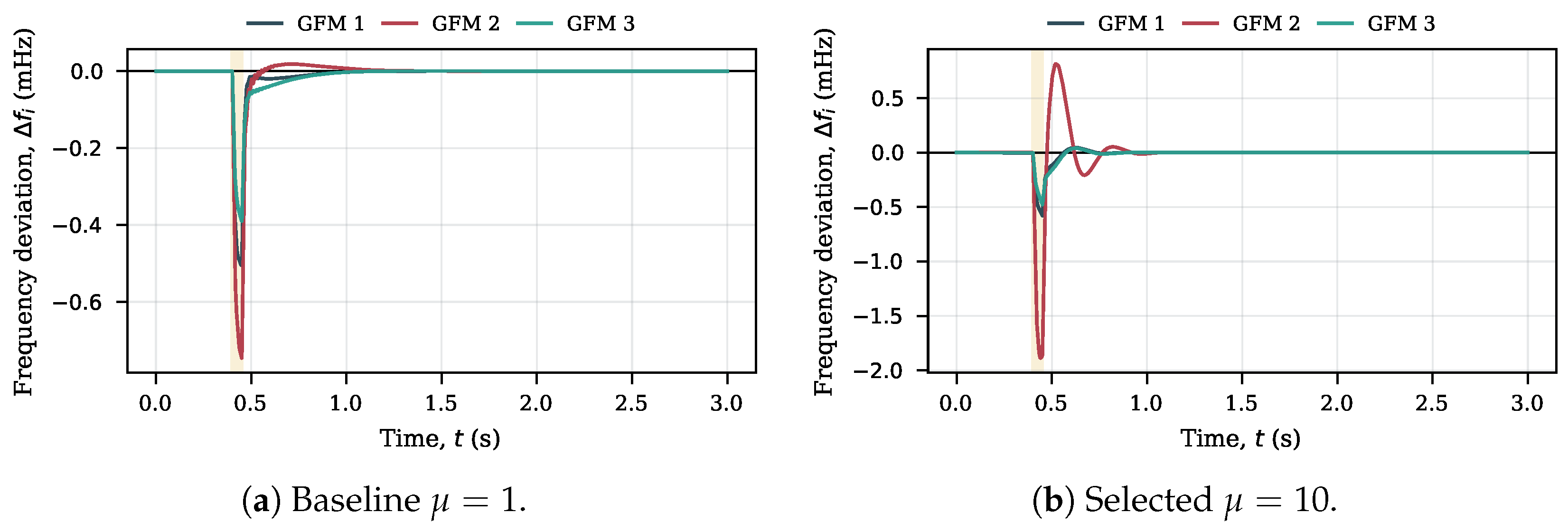
The full-order screen is used here only to select stable operating settings. In the principal active branch, the real part of the rightmost finite eigenvalue is $-5.95$ s⁻¹ at the baseline $\mu =1$ and $-9.23$ s⁻¹ at the selected $\mu =10$. The corresponding time-domain fitted decay rates are also $-5.95$ and $-9.23$ s⁻¹. Figure 10 applies the same small load pulse to both settings. Every terminal-frequency deviation returns to zero, and the current-reference limiter remains inactive. The selected setting has the faster principal decay but a larger initial frequency excursion, 1.89 mHz rather than 0.75 mHz, so the gain choice remains a damping–excursion tradeoff rather than a rule to maximize $\mu$.

Table 4. Stable CA-PF time-domain fitted decay rates across active sets.

Active Constraint	GFM 1 Upper	GFM 2 Upper	GFM 3 Upper	GFM 1+2 Upper	GFM 3 Lower
${\alpha }_{\mathrm{fit}}(\mu =1)$ [s−1]	$-6.23$	$-5.95$	$-6.57$	$-7.36$	$-7.06$
${\alpha }_{\mathrm{fit}}(\mu =10)$ [s−1]	$-9.83$	$-9.23$	$-10.3$	$-6.85$	$-11.05$

extends the check to five active sets. Every time-domain fitted decay rate is negative at both settings. The selected value increases the decay rate in four cases and remains strongly negative in the joint GFM 1/2 case. The 86.4 screen ceiling is therefore retained as an admissibility limit, not used as a performance target. Every reported trajectory decays.

9. Discussion

Every operating condition reported in the case studies is stable under both eigenvalue analysis and nonlinear simulation. The baseline and selected CA-PF settings give negative rightmost-eigenvalue real parts and negative time-domain fitted decay rates across all five tested active sets. This evidence verifies the selected parameter range without attributing a new adverse local dynamic mechanism to PF or CA-PF. Proposition 5 further shows that the proposed finite-amplitude paths introduce no new first-order local mode on the strict active branch. The fixed common channels parameterized by $K_R$ and $K_D$ remain separate from $R_c$, which is zero in normal operation, driven by $P_e-P_{\max }$, bounded, and transient.

Robustness has two distinct meanings in this comparison. Locally, CA-PF has exactly the same strict active-branch linearization as PF, while PL requires its own generalized-slope screen. For finite disturbances, Table 3 shows that CA-PF retains positive peak and energy reductions relative to both nearly coincident PL and PF baselines across operating-point, plant, network, controller, and measurement variations. The bounded fast action and the quadratic noise bound in (34) explain why this sensitivity is gradual. They do not establish robustness outside the tested parameter set.

The inactive current limiter has a separate interpretation in the overload study. Its largest current request is approximately 0.6 p.u. against a 2 p.u. limit, so the central event is not an AC overcurrent event. It is deliberately a source-limited operating condition in which the available active power, 174 MW, is below the converter’s transient current capability. The three-GFM trajectory extends this interpretation. GFM 2 first reaches its declared source ceiling, then GFMs 2 and 3 become constrained together, and GFM 1 supplies the remaining feasible imbalance. Reversing the load sequence releases the constraints in the opposite order without current-limiter engagement. The source audit then gives the per-unit violation a physical test. PF crosses a declared DC-voltage floor, while CA-PF avoids it over the nonempty range $15.8<H_{\mathrm{dc}}<33.9$ ms. Changing units alone would not establish this outcome.

The audit also limits the claim. It assumes a lossless averaged bridge, no recharge credit, and no feedback before protection pickup. It does not establish battery state-of-charge, thermal damage, fuel-cell stress, or the post-trip response. A technology-specific application must replace (5) with its DC source, regulator, and protection logic. The supported controller and stability claims remain local to the declared fixed branches and mechanism-specific to the tested full-order AC model class. Appendix A shows the second-order structure behind the local-model preservation result, and Appendix B states precisely what the eigenvalue-based screen does and does not imply. Global certificates, simultaneous active-power/current-limit transitions, PWM switching, post-protection DC/AC interaction, unbalanced faults, and EMT or hardware validation remain outside the present scope.

The formulation is benchmark independent, but transfer to another GFM law is conditional rather than automatic. It requires a locally available terminal-power signal, a source-limiting port in the synchronization or power-regulation channel, and a voltage-reference port that accepts the bounded term $-R_c{i}_2$. A virtual synchronous machine (VSM) can place the slow correction in its virtual mechanical-power or swing channel. Dispatchable virtual oscillator control (dVOC) can admit an analogous voltage-vector correction, but its state map, steady-state conditions, and local model differ from those studied here. For either architecture, the boundary identities $\Delta F\left(\overline{x}\right)=0$ and $D\Delta F\left(\overline{x}\right)=0$ and the full-order screen must therefore be re-established. The present numerical evidence is limited to the detailed droop-controlled realization.

CA-PF is decentralized. Each converter uses its own terminal voltage, current, filtered power, and source ceiling, so there is no inter-converter communication delay in the feedback law. Sensor, anti-alias-filter, computation, and actuation delays remain relevant local delays and must be represented in $F_c$ when they are not negligible. A delayed supervisory update of $P_{\max }$ is a separate scheduling issue and is not covered by the present tests.

Three-phase faults and deep voltage sags primarily engage fault-ride-through and current-limiting logic, while converter disconnection changes both topology and power-balance feasibility. These events cannot be interpreted as stronger versions of the load-step test. After a disconnection, a necessary steady-state feasibility condition is

$$\sum _{i\in {\mathcal{C}}_{\mathrm{on}}}{P}_{\max ,i}\ge P_{\mathrm{load}}+P_{\mathrm{loss}},$$

(46)

where ${\mathcal{C}}_{\mathrm{on}}$ is the connected converter set. If this condition fails, no active-power limiter can create a feasible equilibrium. If it holds, the post-event topology, current-limiter mode, and reachable CA-PF active sets require a new hybrid stability screen. Consequently, this paper does not claim fault, sag, or disconnection robustness. Their credible evaluation requires coordinated current limiting, fault-ride-through controls, topology-dependent feasibility checks, and EMT or hardware validation.

10. Conclusions

This paper identified a concrete limitation of PL and PF in a detailed droop-controlled GFM implementation. Their filtered outer power–frequency path does not supply a voltage-reference action for the first electrical power peak. It addressed this limitation with CA-PF, which coordinates a bounded, instantaneous-power-triggered resistance path with a shaped PF multiplier. Both paths vanish to first order at the binding constraint, so the corresponding PF equilibrium and active-branch Jacobian are preserved.

The full-order comparison changes the conclusion available from PL/PF alone. On the 300 MVA monitored converter, CA-PF reduces the peak exceedance from 5.41 to 2.45 MW, a 54.7% reduction, and reduces excess energy by 53.4%. At a 0.95 p.u. DC-voltage floor, the audited buffer requirement falls from 33.9 ms for PF to 15.8 ms for CA-PF. The independent current limiter remains inactive, confirming that this result concerns source power rather than AC overcurrent. The component study explains the mechanism. Shaping alone cannot change the filtered first peak, whereas resistance alone does not reduce sustained exposure. Both metrics improve across seven droop-controlled GFM scenarios.

Full-order screening confirms that the baseline and selected CA-PF gains retain negative rightmost-eigenvalue real parts across the declared active branches, and the corresponding nonlinear perturbations decay. The CA-PF-only network study confirms the active-set sequence from one constrained source to two constrained sources and back, while the remaining converter supplies the feasible imbalance. It also makes the instantaneous/filtered power separation and the resulting fast/slow actions visible in one trajectory. The source-buffer result is a pre-trip exposure audit, not a universal DC-source claim.

The present scope is limited to local fixed-branch analysis and balanced averaged-model validation on the studied three-converter network. Future work will address finite-amplitude certification, broader multi-converter validation, and EMT or hardware implementation.

References

1. Milano, F.; Dörfler, F.; Hug, G.; Hill, D.J.; Verbič, G. Foundations and Challenges of Low-Inertia Systems (Invited Paper). In Proceedings of the 2018 Power Systems Computation Conference (PSCC); IEEE: New York, NY, USA, 2018; pp. 1–25. [Google Scholar] [CrossRef] [Scilit]
2. Marković, U.; Stanojev, O.; Aristidou, P.; Vrettos, E.; Callaway, D.S.; Hug, G. Understanding Small-Signal Stability of Low-Inertia Systems. IEEE Trans. Power Syst. 2021, 36, 3997–4017. [Google Scholar] [CrossRef] [Scilit]
3. Subotić, I.; Groß, D.; Colombino, M.; Dörfler, F. A Lyapunov Framework for Nested Dynamical Systems on Multiple Time Scales With Application to Converter-Based Power Systems. IEEE Trans. Autom. Control 2021, 66, 5909–5924. [Google Scholar] [CrossRef] [Scilit]
4. Lasseter, R.H. Microgrids. In Proceedings of the 2002 IEEE Power Engineering Society Winter Meeting; IEEE: New York, NY, USA, 2002; Volume 1, pp. 305–308. [Google Scholar] [CrossRef] [Scilit]
5. Simpson-Porco, J.W.; Dörfler, F.; Bullo, F. Synchronization and Power Sharing for Droop-Controlled Inverters in Islanded Microgrids. Automatica 2013, 49, 2603–2611. [Google Scholar] [CrossRef] [Scilit]
6. Johnson, B.B.; Dhople, S.V.; Hamadeh, A.O.; Krein, P.T. Synchronization of Nonlinear Oscillators in an LTI Electrical Power Network. IEEE Trans. Circuits Syst. I 2014, 61, 834–844. [Google Scholar] [CrossRef] [Scilit]
7. Arghir, C.; Jouini, T.; Dörfler, F. Grid-Forming Control for Power Converters Based on Matching of Synchronous Machines. Automatica 2018, 95, 273–282. [Google Scholar] [CrossRef] [Scilit]
8. Tayyebi, A.; Groß, D.; Anta, A.; Kupzog, F.; Dörfler, F. Frequency Stability of Synchronous Machines and Grid-Forming Power Converters. IEEE J. Emerg. Sel. Top. Power Electron. 2020, 8, 1004–1018. [Google Scholar] [CrossRef] [Scilit]
9. Xu, Y.; Qu, Z.; Qi, J. State-Constrained Grid-Forming Inverter Control for Robust Operation of AC Microgrids. In Proceedings of the 2020 European Control Conference (ECC); IEEE: New York, NY, USA, 2020; pp. 471–474. [Google Scholar] [CrossRef] [Scilit]
10. Hart, P.J.; Gong, M.; Liu, H.; Chen, Z.; Zhang, Y.; Wang, Y. Provably-Stable Overload Ride-Through Control for Grid-Forming Inverters Using System-Wide Lyapunov Function Analysis. IEEE Trans. Energy Convers. 2022, 37, 2761–2776. [Google Scholar] [CrossRef] [Scilit]
11. Baier, C.R.; Melin, P.E.; Torres, M.A.; Ramirez, R.O.; Muñoz, C.; Quinteros, A. Developing and Evaluating the Operating Region of a Grid-Connected Current Source Inverter from Its Mathematical Model. Mathematics 2024, 12, 1775. [Google Scholar] [CrossRef] [Scilit]
12. Groß, D.; Dörfler, F. Projected Grid-Forming Control for Current-Limiting of Power Converters. In Proceedings of the 2019 57th Annual Allerton Conference on Communication, Control, and Computing (Allerton); IEEE: New York, NY, USA, 2019; pp. 326–333. [Google Scholar] [CrossRef] [Scilit]
13. Baeckeland, N.; Chatterjee, D.; Lu, M.; Johnson, B.B.; Seo, G.S. Overcurrent Limiting in Grid-Forming Inverters: A Comprehensive Review and Discussion. IEEE Trans. Power Electron. 2024, 39, 14493–14517. [Google Scholar] [CrossRef] [Scilit]
14. Askarov, A.; Radko, P.; Bay, Y.; Gusarov, I.; Kabirov, V.; Ilyushin, P.; Suvorov, A. Overcurrent Limiting Strategy for Grid-Forming Inverters Based on Current-Controlled VSG. Mathematics 2025, 13, 3207. [Google Scholar] [CrossRef] [Scilit]
15. Du, W.; Lasseter, R.H.; Khalsa, A.S. Survivability of Autonomous Microgrid During Overload Events. IEEE Trans. Smart Grid 2019, 10, 3515–3524. [Google Scholar] [CrossRef] [Scilit]
16. Du, W. Model Specification of Droop-Controlled, Grid-Forming Inverters (REGFM_A1); Technical Report PNNL-35110; Pacific Northwest National Laboratory: Richland, WA, USA, 2023. [CrossRef] [Scilit]
17. Iraniparast, A.; Groß, D. Networked Dynamics with Application to Frequency Stability of Grid-Forming Power-Limiting Droop Control. IEEE Trans. Control Netw. Syst. 2025, 12, 2856–2867. [Google Scholar] [CrossRef] [Scilit]
18. Iraniparast, A.; Groß, D. Stability and Convergence of Multi-Converter Systems Using Projection-Free Power-Limiting Droop Control. arXiv 2026, arXiv:2602.16036. [Google Scholar]
19. Tang, Y.; Qu, G.; Li, N. Semi-Global Exponential Stability of Augmented Primal–Dual Gradient Dynamics for Constrained Convex Optimization. Syst. Control Lett. 2020, 144, 104754. [Google Scholar] [CrossRef] [Scilit]
20. Groß, D.; Colombino, M.; Brouillon, J.S.; Dörfler, F. The Effect of Transmission-Line Dynamics on Grid-Forming Dispatchable Virtual Oscillator Control. IEEE Trans. Control Netw. Syst. 2019, 6, 1148–1160. [Google Scholar] [CrossRef] [Scilit]
21. Häberle, V.; He, X.; Huang, L.; Dörfler, F.; Low, S.H. Decentralized Parametric Stability Certificates for Grid-Forming Converter Control. arXiv 2025, arXiv:2503.05403. [Google Scholar]
22. Askarov, A.; Bay, Y.; Ufa, R.; Radko, P.; Ilyushin, P.; Suvorov, A. Signatures and Mechanism Analysis of Converter-Grid Subsynchronous Oscillations. Mathematics 2024, 12, 3884. [Google Scholar] [CrossRef] [Scilit]
23. Rosso, R.; Wang, X.; Liserre, M.; Lu, X.; Engelken, S. Grid-Forming Converters: Control Approaches, Grid-Synchronization, and Future Trends: A Review. IEEE Open J. Ind. Appl. 2021, 2, 93–109. [Google Scholar] [CrossRef] [Scilit]
24. Kenyon, R.W.; Sajadi, A.; Hodge, B.M. Autonomous Grid-Forming Inverter Exponential Droop Control for Improved Frequency Stability. Int. J. Electr. Power Energy Syst. 2025, 172, 111160. [Google Scholar] [CrossRef] [Scilit]
25. Me, S.P.; Zabihi, S.; Blaabjerg, F.; Bahrani, B. Adaptive Virtual Resistance for Postfault Oscillation Damping in Grid-Forming Inverters. IEEE Trans. Power Electron. 2022, 37, 3813–3824. [Google Scholar] [CrossRef] [Scilit]
26. Zhou, X.; Zhang, L.; Peng, H.; Hong, L.; Xu, Q.; Zhang, Z.; Shao, J.; Ma, J.; Hu, Y. An Improved Grid-Forming Control Method With Adaptive Virtual Impedance Combining Current Limitation and Transient Stability Improvement. Int. J. Electr. Power Energy Syst. 2026, 175, 111659. [Google Scholar] [CrossRef] [Scilit]
27. Askarov, A.; Rudnik, V.; Ruban, N.; Radko, P.; Ilyushin, P.; Suvorov, A. Enhanced Virtual Synchronous Generator with Angular Frequency Deviation Feedforward and Energy Recovery Control for Energy Storage System. Mathematics 2024, 12, 2691. [Google Scholar] [CrossRef] [Scilit]
28. Dupuis, P.; Nagurney, A. Dynamical Systems and Variational Inequalities. Ann. Oper. Res. 1993, 44, 7–42. [Google Scholar] [CrossRef] [Scilit]
29. Yazdani, A.; Iravani, R. Voltage-Sourced Converters in Power Systems: Modeling, Control, and Applications; Wiley: Hoboken, NJ, USA, 2010. [Google Scholar]
30. Gajare, P.M.; Benzaquen, J.; Divan, D. Grid-Forming Controller With Enhanced Disturbance Rejection. IEEE J. Emerg. Sel. Top. Power Electron. 2025, 13, 5201–5217. [Google Scholar] [CrossRef] [Scilit]
31. Clarke, F.H. Optimization and Nonsmooth Analysis; Society for Industrial and Applied Mathematics: Philadelphia, PA, USA, 1990. [Google Scholar] [CrossRef] [Scilit]
32. Khalil, H.K. Nonlinear Systems, 3rd ed.; Prentice-Hall: Upper Saddle River, NJ, USA, 2002. [Google Scholar]
33. Kunkel, P.; Mehrmann, V. Differential-Algebraic Equations: Analysis and Numerical Solution; European Mathematical Society: Zürich, Switzerland, 2006. [Google Scholar] [CrossRef] [Scilit] [PubMed]
34. Zimmerman, R.D.; Murillo-Sánchez, C.E.; Thomas, R.J. MATPOWER: Steady-State Operations, Planning, and Analysis Tools for Power Systems Research and Education. IEEE Trans. Power Syst. 2011, 26, 12–19. [Google Scholar] [CrossRef] [Scilit]
Figure 1. Study foundations showing constraint geometry, the averaged grid-forming converter (GFM) network port, and the separated constraint-activated projection-free (CA-PF) paths.
Mathematics 14 03037 g001
Figure 2. Converter signal flow with the filtered slow limiter and instantaneous CA-PF voltage-reference path.
Mathematics 14 03037 g002
Figure 3. Signal-level comparison of the PL , PF , and proposed CA - PF upper-limit branches.
Mathematics 14 03037 g003
Figure 4. Kron-reduced dynamic validation network and declared source ceilings.
Mathematics 14 03037 g004
Figure 5. Central overload, accumulated exposure, component study, and transient voltage effect.
Mathematics 14 03037 g005
Figure 6. One-way source-buffer audit of the verified active-power trajectories.
Mathematics 14 03037 g006
Figure 7. Matched PL, PF, and proposed CA-PF comparison of peak and violation area.
Mathematics 14 03037 g007
Figure 8. Finite-amplitude sweep used to select the resistance ceiling.
Mathematics 14 03037 g008
Figure 9. Sequential activation and release of two CA-PF source ceilings.
Mathematics 14 03037 g009
Figure 10. Stable CA-PF responses under an identical small load pulse.
Mathematics 14 03037 g010