A Blaschke-Type Covering Formula in Dimensions Higher than Two via Lattice Voronoi Cells

Abstract

Let $K\subset {\mathbb{R}}^n$ be a bounded convex body. We prove a lattice-averaging formula that gives upper bounds for the number of unit balls required to cover K. If the Voronoi cell P of a lattice is contained in the Euclidean unit ball, then some translate and rotation of the lattice produces a covering whose size is at most a linear combination of the intrinsic volumes of K; the coefficients are determined by the intrinsic volumes of P. The proof averages the number of Voronoi cells meeting K over one fundamental cell and over $SO\left(n\right)$. For the regular hexagonal lattice in ${\mathbb{R}}^2$, the formula reproduces the classical planar Blaschke bound. For the cubic lattice, it gives a closed-form estimate in every dimension $n\ge 2$. In ${\mathbb{R}}^3$, explicit computations for the cubic, face-centered cubic, and body-centered cubic Voronoi cells show that the body-centered cubic lattice has the smallest coefficientwise bound among these three lattices. In ${\mathbb{R}}^4$, the intrinsic volumes of the $A_4^{\ast }$ permutohedron are computed from its graphical-zonotope representation, leading to a sharper bound than for the cubic lattice.

1. Introduction

1.1. Problem Setting and Previous Work

Coverage questions arise whenever a finite collection of range-limited devices must serve an entire region. Recent examples occur in rather different settings: ultra-wideband anchor placement, where configurations are optimized under complete-coverage constraints [1]; cooperative multi-UAV search, where coverage rate is balanced against energy consumption [2]; and satellite-constellation design, where coverage and revisit requirements are balanced against the number of spacecraft [3]. These models also involve dynamics, obstacles, communication constraints, and other features that are deliberately absent from the present setting. At the geometric level, however, they share a basic question: how many congruent range sets are sufficient to cover a prescribed region? Exact covering numbers are difficult to determine even for simple bodies, so explicit upper bounds provide both a resource guarantee and a way to compare structured placements.

A convex body is a compact convex set with nonempty interior. For a convex body $K\subset {\mathbb{R}}^n$, define

$$N\left(K\right):=\min \left\{m:K\subseteq {\displaystyle \bigcup _{i=1}^m}(x_i+B^n)\mathrm{for}\mathrm{some}{x}_1,\dots ,x_m\in {\mathbb{R}}^n\right\},$$

(1)

where $B^n$ is the Euclidean unit ball centered at the origin. Thus, $N\left(K\right)$ is the least number of unit balls needed to cover K. This is a special case of covering a convex body by translates of another convex body; see Rogers [4], Rogers and Zong [5], Gruber [6], Zong [7], and the survey by Naszódi [8]. More generally, if $N(K,L)$ is the least number of translates of a convex body L that cover K, and $\theta \left(L\right)$ is the translative covering density of L, the Rogers–Zong estimate states that

$$N(K,L)\le \theta \left(L\right){\displaystyle \frac{V_n(K-L)}{V_n\left(L\right)}},K-L:=K+(-L).$$

A related line of work concerns lattice coverings of the whole space. Standard references include Conway and Sloane [9]; computational methods are developed by Schürmann and Vallentin [10], and recent general bounds are due to Ordentlich, Regev, and Weiss [11].

A full-rank lattice is a discrete subgroup $\Lambda \subset {\mathbb{R}}^n$ generated by a basis of ${\mathbb{R}}^n$. For $x\in \Lambda$, its Voronoi cell is

$${\mathrm{Vor}}_{\Lambda }\left(x\right):=\{y\in {\mathbb{R}}^n: \parallel y-x\parallel \le \parallel y-z\parallel \mathrm{for}\mathrm{every}z\in \Lambda \}.$$

(2)

The point x is the center of the cell. All cells are translates of the centrally symmetric polytope $P:={\mathrm{Vor}}_{\Lambda }\left(0\right)$, and the family $P+\lambda$, $\lambda \in \Lambda$, tiles ${\mathbb{R}}^n$. For background on Voronoi cells and tessellations, see [12,13]. Their polyhedral representations and extension complexity are studied in [14]; related intrinsic-volume questions for parallelohedra and zonotopes appear in [15,16].

In the plane, one form of the Blaschke covering formula states that if $K\subset {\mathbb{R}}^2$ has area $A\left(K\right)$ and perimeter $L\left(K\right)$, then

$$N\left(K\right)\le {\displaystyle \frac{2}{3\sqrt{3}}}A\left(K\right)+{\displaystyle \frac{2}{\pi \sqrt{3}}}L\left(K\right)+1,$$

(3)

see Fejes Tóth [17] and the related discussion in Gul, Cohen, and Haber [18]. A standard proof uses the regular hexagonal Voronoi tiling: one averages the number of hexagons intersecting a random placement of K, and then replaces each intersected hexagon by its circumscribed unit disc. A spherical analogue on $S^2$ was established in [19].

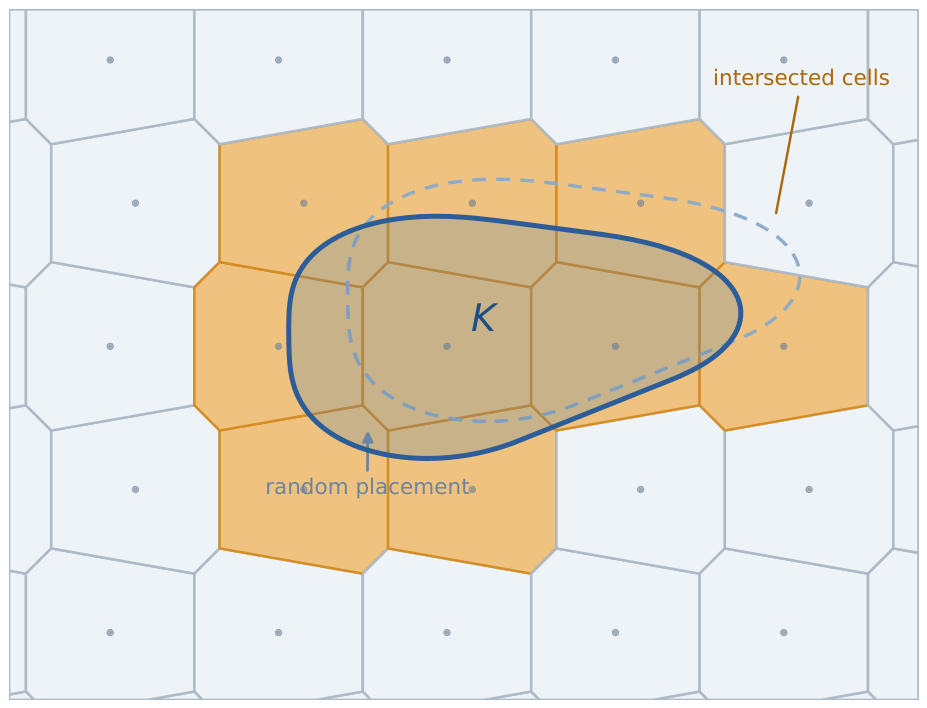
The purpose of this paper is to develop a Euclidean counterpart in higher dimensions. The role of the regular hexagon is played by a lattice Voronoi cell P, normalized so that its covering radius is one, equivalently $P\subseteq B^n$. The role of planar mixed-area identities is played by intrinsic volumes and the rotational kinematic formula. Figure 1 illustrates the geometric mechanism.

1.2. Gap, Assumptions, and Contributions

General covering-number estimates, such as those in [5,8], allow arbitrary translates and are usually stated in terms of volume or covering density. Lattice-covering density, on the other hand, concerns a covering of the whole space. These viewpoints leave a natural intermediate question for a finite body: if the centers are constrained to one lattice, how do the different intrinsic volumes of K enter the covering count? The formula proved below answers this question coefficient by coefficient; the coefficients are themselves intrinsic-volume data of the lattice Voronoi cell.

Throughout the paper, the admissible centers form a single rigid motion $t+\gamma \Lambda$ of a full-rank lattice $\Lambda$. Its Voronoi cell is scaled so that $P\subseteq B^n$, equivalently so that the covering radius is at most one. This restriction produces an explicit structured covering, but it is important to keep its scope in view: no claim is made that the resulting covering is optimal among all possible placements of unit balls.

The resulting contributions are as follows.

• We prove a lattice-averaging identity over one fundamental domain and the rotation group, without a large-window limit or boundary-error term.
• We show that the general formula recovers the planar Blaschke estimate (3) from the regular hexagonal lattice.
• For the cubic lattice, we obtain a closed-form bound in every dimension $n\ge 2$.
• In ${\mathbb{R}}^3$, we compute all required geometric quantities explicitly for the cubic, face-centered cubic (fcc), and body-centered cubic (bcc) Voronoi cells. The bcc lattice gives the smallest coefficientwise bound among these three.
• In ${\mathbb{R}}^4$, we represent the $A_4^{\ast }$ Voronoi cell as a graphical zonotope, compute its intrinsic volumes by enumerating forests of the complete graph $K_5$, and obtain a sharper bound than for the cubic lattice.

The paper is organized as follows. Section 2 establishes notation and records the standard integral-geometric tools. Section 3 presents the averaging argument and recovers the planar formula. Section 4 treats the cubic lattice in arbitrary dimension. Section 5 gives the three-dimensional calculations and comparison. Section 6 treats the $A_4^{\ast }$ lattice. Section 7 discusses the relation with previous covering estimates, summarizes the conclusions, and lists open problems.

2. Preliminaries

2.1. Convex-Geometric Notation and Intrinsic Volumes

Let ${\mathcal{K}}^n$ denote the family of nonempty compact convex sets in ${\mathbb{R}}^n$. The Minkowski sum of sets $K,M\subseteq {\mathbb{R}}^n$ is

$$K+M:=\{x+y:x\in K,y\in M\}.$$

We write ${\kappa }_m:=V_m\left(B^m\right)={\pi }^{m/2}/\Gamma (1+m/2)$ for the volume of the m-dimensional unit ball. The support function of $K\in {\mathcal{K}}^n$ is

$$h_K\left(u\right):=\underset{x\in K}{\max }\langle x,u\rangle ,u\in S^{n-1}.$$

Its width in direction u is $h_K\left(u\right)+h_K(-u)$, and its mean width is

$$W\left(K\right):={\displaystyle \frac{1}{n{\kappa }_n}}{\int }_{S^{n-1}}\left(h_K\left(u\right)+h_K(-u)\right)du.$$

(4)

The following standard results are recalled from Schneider [20]; see also Gardner [21].

Theorem 1 

(Steiner formula). For $K\in {\mathcal{K}}^n$ and $r\ge 0$,

$$V_n(K+r{B}^n)={\displaystyle \sum _{j=0}^n}{\kappa }_{n-j}{V}_j\left(K\right)r^{n-j}.$$

(5)

The coefficients $V_j\left(K\right)$ are the intrinsic volumes of K.

Our normalization is

$$V_n\left(K\right)=V\left(K\right),2V_{n-1}\left(K\right)=A\left(K\right),V_0\left(K\right)=1,$$

(6)

and

$$V_1\left(K\right)={\displaystyle \frac{n{\kappa }_n}{2{\kappa }_{n-1}}}W\left(K\right).$$

(7)

Thus, $V\left(K\right)$ is n-dimensional volume, $A\left(K\right)$ is $(n-1)$-dimensional surface area, and $W\left(K\right)$ is mean width as defined in (4).

For a polytope Q and a proper k-face F, let $L\left(F\right):=\mathrm{lin}(F-F)$ be the linear subspace parallel to F, and let $N(Q,F)\subseteq L{\left(F\right)}^{\perp }$ be the outer normal cone at F. The outer angle $\gamma (Q,F)$ is the spherical measure of $N(Q,F)\cap S^{n-k-1}$, divided by the total spherical measure of the unit sphere in $L{\left(F\right)}^{\perp }$; for the top-dimensional face we set $\gamma (Q,Q)=1$. Then

$$V_k\left(Q\right)=\sum _{F\in {\mathcal{F}}_k\left(Q\right)}\gamma (Q,F)V_k\left(F\right),$$

(8)

where ${\mathcal{F}}_k\left(Q\right)$ is the family of k-faces and $V_k\left(F\right)$ denotes their k-dimensional volume.

In dimension three, a useful specialization is the edge formula

$$W\left(Q\right)={\displaystyle \frac{1}{4\pi }}\sum _{e\in {\mathcal{F}}_1\left(Q\right)}\mathsf{\ell }\left(e\right)\alpha \left(e\right),$$

(9)

where $\mathsf{\ell }\left(e\right)$ is the length of e and $\alpha \left(e\right)$ is the exterior dihedral angle, equivalently the angle between the two outward unit normals of the adjacent facets.

2.2. Lattices and Voronoi Cells

Let $\Lambda \subset {\mathbb{R}}^n$ be a full-rank lattice and let $P={\mathrm{Vor}}_{\Lambda }\left(0\right)$ be the Voronoi cell defined in (2). The cell P is centrally symmetric: if $x\in P$, then for every $\lambda \in \Lambda$,

$$\parallel -x\parallel =\parallel x\parallel \le \parallel x+\lambda \parallel =\parallel -x-\lambda \parallel ,$$

so $-x\in P$. The sets $P+\lambda$, $\lambda \in \Lambda$, tile ${\mathbb{R}}^n$ up to common boundaries. Consequently, the covolume of $\Lambda$ equals $V_n\left(P\right)$.

The covering radius of $\Lambda$ is

$$\mu (\Lambda ):=\underset{x\in P}{\max }\parallel x\parallel .$$

After scaling, the condition $\mu (\Lambda )=1$ is equivalent to $P\subseteq B^n$ with at least one vertex on $S^{n-1}$. In this normalization, every cell $P+\lambda$ is contained in the unit ball $B^n+\lambda$ centered at its lattice point.

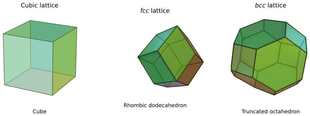
For background on Voronoi tessellations, see [12,13]; for translative tilings, see Grünbaum and Shephard [22]. In ${\mathbb{R}}^3$, the cubic lattice has a cube as Voronoi cell, the fcc lattice has a rhombic dodecahedron, and the bcc lattice has a truncated octahedron [9].

2.3. Rotational Averaging

Let $SO\left(n\right)$ be the special orthogonal group, equipped with its normalized Haar probability measure $d\gamma$. The following rotational formula is standard in integral geometry; see Schneider and Weil [23].

Theorem 2 

(Rotational kinematic formula). For $K,M\in {\mathcal{K}}^n$,

$${\int }_{SO\left(n\right)}{V}_n(K+\gamma M)d\gamma ={\displaystyle \sum _{j=0}^n}{c}_{n,j}{V}_j\left(K\right)V_{n-j}\left(M\right),$$

(10)

where

$$c_{n,j}:={\displaystyle \frac{j!{\kappa }_j(n-j)!{\kappa }_{n-j}}{n!{\kappa }_n}}.$$

(11)

Formula (10) writes the rotational average of the Minkowski-sum volume as a bilinear combination of intrinsic volumes. The endpoint coefficients satisfy $c_{n,0}=c_{n,n}=1$.

Lemma 1 

(Intersection criterion). For arbitrary sets $A,B\subset {\mathbb{R}}^n$ and vectors $a,b\in {\mathbb{R}}^n$,

$$(A+a)\cap (B+b)\ne ⌀⟺b-a\in A+(-B).$$

(12)

Proof. 

The intersection is nonempty precisely when there exist $x\in A$ and $y\in B$ with $x+a=y+b$, which is equivalent to $b-a=x-y\in A+(-B)$. □

3. A Blaschke-Type Lattice-Averaging Principle

The proof follows six steps.

• Choose a lattice $\Lambda$ whose Voronoi cell P satisfies $P\subseteq B^n$.
• Rotate the entire lattice by $\gamma \in SO\left(n\right)$.
• Translate it by a vector t chosen in one fundamental cell $\gamma P$.
• Count the transformed Voronoi cells intersecting K.
• Average that count first over t and then over $\gamma$.
• Choose a placement no worse than the average and replace every intersected cell by its containing unit ball.

Proposition 1 

(General lattice bound). Let $K\in {\mathcal{K}}^n$, and let $P={\mathrm{Vor}}_{\Lambda }\left(0\right)$ be the Voronoi cell of a full-rank lattice $\Lambda \subset {\mathbb{R}}^n$. If $P\subseteq B^n$, then there exist $\gamma \in SO\left(n\right)$ and $t\in {\mathbb{R}}^n$ such that K is covered by at most

$${\mathcal{B}}_P\left(K\right):={\displaystyle \sum _{j=0}^n}{c}_{n,j}{\displaystyle \frac{V_{n-j}\left(P\right)}{V_n\left(P\right)}}{V}_j\left(K\right)$$

(13)

unit balls centered at points of the transformed lattice $t+\gamma \Lambda$.

Proof. 

Fix a rotation $\gamma \in SO\left(n\right)$. For $t\in \gamma P$, define

$$N(t,\gamma ):=\#\left\{\lambda \in \Lambda :K\cap \left(t+\gamma \lambda +\gamma P\right)\ne ⌀\right\}.$$

(14)

Because K and P are compact, only finitely many lattice points contribute to this count. By Lemma 1,

$$K\cap \left(t+\gamma \lambda +\gamma P\right)\ne ⌀⟺t+\gamma \lambda \in K+(-\gamma P).$$

Since $P=-P$, this is equivalent to $t+\gamma \lambda \in K+\gamma P$. Hence

$$N(t,\gamma )=\sum _{\lambda \in \Lambda }{\mathbf{1}}_{K+\gamma P}(t+\gamma \lambda ),$$

where ${\mathbf{1}}_S$ is the indicator function of S.

Average over the fundamental cell $\gamma P$. The translates $\gamma P+\gamma \lambda$, $\lambda \in \Lambda$, tile ${\mathbb{R}}^n$, so Tonelli’s theorem and the change of variables $x=t+\gamma \lambda$ give

$$\begin{array}{cc}\hfill {\displaystyle \frac{1}{V_n\left(P\right)}}{\int }_{\gamma P}N(t,\gamma )dt& ={\displaystyle \frac{1}{V_n\left(P\right)}}\sum _{\lambda \in \Lambda }{\int }_{\gamma P}{\mathbf{1}}_{K+\gamma P}(t+\gamma \lambda )dt\hfill \\ \hfill & ={\displaystyle \frac{1}{V_n\left(P\right)}}{\int }_{{\mathbb{R}}^n}{\mathbf{1}}_{K+\gamma P}\left(x\right)dx\hfill \\ \hfill & ={\displaystyle \frac{V_n(K+\gamma P)}{V_n\left(P\right)}}.\hfill \end{array}$$

(15)

Now choose $\gamma$ according to normalized Haar measure on $SO\left(n\right)$ and, independently, choose s uniformly in P; set $t:=\gamma s$. Conditional on $\gamma$, the vector t is uniform in the fundamental cell $\gamma P$. Averaging (15) over $\gamma$ therefore gives

$$\mathbb{E}N(\gamma s,\gamma )={\displaystyle \frac{1}{V_n\left(P\right)}}{\int }_{SO\left(n\right)}{V}_n(K+\gamma P)d\gamma .$$

(16)

Applying Theorem 2 to (16) gives the right-hand side of (13). Since this quantity is the average of $N(\gamma s,\gamma )$, there is a pair $(s,\gamma )$, and hence $(t,\gamma )$ with $t=\gamma s$, for which $N(t,\gamma )\le {\mathcal{B}}_P\left(K\right)$.

For this placement, every point of K lies in a transformed Voronoi cell counted by $N(t,\gamma )$. Because $P\subseteq B^n$, each such cell $t+\gamma \lambda +\gamma P$ is contained in the unit ball $t+\gamma \lambda +B^n$. The unit balls centered at the corresponding lattice points therefore cover K. □

Remark 1. 

The covering constructed in the proof uses an integer number $N(t,\gamma )$ of balls, with $N(t,\gamma )\le {\mathcal{B}}_P\left(K\right)$. Hence it uses at most $\lfloor {\mathcal{B}}_P\left(K\right)\rfloor$ balls, and in particular

$$N\left(K\right)\le ⌊{\mathcal{B}}_P\left(K\right)⌋.$$

We keep the real-valued expression ${\mathcal{B}}_P\left(K\right)$ because the comparisons below concern its coefficients.

Corollary 1 

(Recovery of the planar Blaschke formula). For the regular hexagonal lattice in ${\mathbb{R}}^2$, normalized so that the Voronoi hexagon has circumradius one, Proposition 1 gives (3).

Proof. 

Let H be the regular hexagon of side length one. Then

$$V_2\left(H\right)={\displaystyle \frac{3\sqrt{3}}{2}},V_1\left(H\right)={\displaystyle \frac{\mathrm{per}\left(H\right)}{2}}=3,V_0\left(H\right)=1.$$

For $n=2$, $c_{\mathrm{2,0}}=c_{\mathrm{2,2}}=1$ and $c_{\mathrm{2,1}}=2/\pi$. Moreover, $V_2\left(K\right)=A\left(K\right)$ and $V_1\left(K\right)=L\left(K\right)/2$. Substitution in (13) gives

$$\begin{array}{cc}\hfill {\mathcal{B}}_H\left(K\right)& =1+{\displaystyle \frac{2}{\pi }}{\displaystyle \frac{3}{3\sqrt{3}/2}}{\displaystyle \frac{L\left(K\right)}{2}}+{\displaystyle \frac{1}{3\sqrt{3}/2}}A\left(K\right)\hfill \\ \hfill & =1+{\displaystyle \frac{2}{\pi \sqrt{3}}}L\left(K\right)+{\displaystyle \frac{2}{3\sqrt{3}}}A\left(K\right),\hfill \end{array}$$

which is (3). □

Remark 2 

(Relation with volumetric covering estimates). For a fixed lattice, (13) is the average number of cells meeting K. Since $P\subseteq B^n$, monotonicity of volume gives

$${\mathcal{B}}_P\left(K\right)={\displaystyle \frac{1}{V_n\left(P\right)}}{\int }_{SO\left(n\right)}{V}_n(K+\gamma P)d\gamma \le {\displaystyle \frac{V_n(K+B^n)}{V_n\left(P\right)}}.$$

(17)

Thus the use of the actual Voronoi cell improves, or leaves unchanged, the estimate obtained by replacing it with the unit ball before averaging.

The coefficient of $V_n\left(K\right)$ is $1/V_n\left(P\right)$. If $\theta (\Lambda ,B^n)={\kappa }_n/V_n\left(P\right)$ is the density of the corresponding lattice covering, this coefficient equals $\theta (\Lambda ,B^n)/{\kappa }_n$. The remaining coefficients depend on the lower intrinsic volumes of P, which are not recorded by covering density. For comparison, the Rogers–Zong estimate with $L=B^n$ has the form $N(K,B^n)\le \theta \left(B^n\right)V_n(K+B^n)/{\kappa }_n$ and allows unrestricted centers. The right-hand side of (17) is its analogue for the prescribed lattice. The two estimates therefore concern different classes of coverings.

4. The Cubic Lattice in ${\mathbb{R}}^{\mathit{n}}$

The Voronoi cell of the cubic lattice is an n-dimensional cube centered at the origin. When this cube is inscribed in the unit sphere, its side length is

$$a={\displaystyle \frac{2}{\sqrt{n}}}.$$

Its intrinsic volumes follow from face counting.

Lemma 2. 

Let $C\subset {\mathbb{R}}^n$ be an n-dimensional cube of side length a. Then, for $0\le k\le n$,

$$V_k\left(C\right)=\left({\displaystyle \genfrac{}{}{0pt}{}{n}{k}}\right)a^k.$$

(18)

In particular, if C is inscribed in the unit sphere, then

$$V_k\left(C\right)=\left({\displaystyle \genfrac{}{}{0pt}{}{n}{k}}\right){\left({\displaystyle \frac{2}{\sqrt{n}}}\right)}^k.$$

(19)

Proof. 

Every k-face of C is a k-cube of volume $a^k$, and there are $2^{n-k}\left({\displaystyle \genfrac{}{}{0pt}{}{n}{k}}\right)$ such faces. The outer angle at each k-face is $2^{k-n}$. Formula (8) therefore gives

$$V_k\left(C\right)=2^{n-k}\left({\displaystyle \genfrac{}{}{0pt}{}{n}{k}}\right)2^{k-n}{a}^k=\left({\displaystyle \genfrac{}{}{0pt}{}{n}{k}}\right)a^k.$$

Substituting $a=2/\sqrt{n}$ proves (19). □

Theorem 3. 

Let $K\in {\mathcal{K}}^n$. Then K can be covered by at most

$$N_C\left(K\right):={\displaystyle \sum _{j=0}^n}{\displaystyle \frac{{\kappa }_j{\kappa }_{n-j}}{{\kappa }_n}}{\left({\displaystyle \frac{\sqrt{n}}{2}}\right)}^j{V}_j\left(K\right)$$

(20)

unit balls centered at the points of a suitable translate and rotation of the n-dimensional cubic lattice.

Proof. 

For the inscribed cube C,

$${\displaystyle \frac{V_{n-j}\left(C\right)}{V_n\left(C\right)}}=\left({\displaystyle \genfrac{}{}{0pt}{}{n}{j}}\right){\left({\displaystyle \frac{\sqrt{n}}{2}}\right)}^j.$$

Substitution in Proposition 1, followed by cancellation of $\left({\displaystyle \genfrac{}{}{0pt}{}{n}{j}}\right)$ with the factorial factor in $c_{n,j}$, gives (20). □

In ${\mathbb{R}}^3$, (20) becomes

$$N_C\left(K\right)={\displaystyle \frac{3\sqrt{3}}{8}}V\left(K\right)+{\displaystyle \frac{9}{16}}A\left(K\right)+{\displaystyle \frac{3\sqrt{3}}{2}}W\left(K\right)+1.$$

(21)

In ${\mathbb{R}}^4$, it gives

$$N_{C,4}\left(K\right)=1+{\displaystyle \frac{16}{3\pi }}{V}_1\left(K\right)+2V_2\left(K\right)+{\displaystyle \frac{16}{3\pi }}{V}_3\left(K\right)+V_4\left(K\right).$$

(22)

5. Three-Dimensional Lattice Bounds

For $n=3$, one has $c_{3,0}=c_{3,3}=1$ and $c_{3,1}=c_{3,2}=1/2$. Moreover, (6) and (7) become

$$V_3\left(Q\right)=V\left(Q\right),V_2\left(Q\right)={\displaystyle \frac{A\left(Q\right)}{2}},V_1\left(Q\right)=2W\left(Q\right),V_0\left(Q\right)=1.$$

Consequently, Proposition 1 specializes as follows.

Corollary 2 

(Three-dimensional cell formula). Let $P\subseteq B^3$ be a lattice Voronoi cell. Then a suitable translate and rotation of the lattice covers $K\in {\mathcal{K}}^3$ with at most

$$1+{\displaystyle \frac{1}{V\left(P\right)}}V\left(K\right)+{\displaystyle \frac{W\left(P\right)}{2V\left(P\right)}}A\left(K\right)+{\displaystyle \frac{A\left(P\right)}{2V\left(P\right)}}W\left(K\right)$$

(23)

unit balls.

Proof. 

Substituting the four three-dimensional identities above into

$${\displaystyle \frac{1}{V\left(P\right)}}{\displaystyle \sum _{j=0}^3}{c}_{3,j}{V}_j\left(K\right)V_{3-j}\left(P\right)$$

gives, term by term,

$$\begin{array}{cc}\hfill & {\displaystyle \frac{V_0\left(K\right)V_3\left(P\right)}{V\left(P\right)}}=1,\hfill \\ \hfill & {\displaystyle \frac{1}{2V\left(P\right)}}{V}_1\left(K\right)V_2\left(P\right)={\displaystyle \frac{1}{2V\left(P\right)}}\left(2W\left(K\right)\right){\displaystyle \frac{A\left(P\right)}{2}}={\displaystyle \frac{A\left(P\right)}{2V\left(P\right)}}W\left(K\right),\hfill \\ \hfill & {\displaystyle \frac{1}{2V\left(P\right)}}{V}_2\left(K\right)V_1\left(P\right)={\displaystyle \frac{1}{2V\left(P\right)}}{\displaystyle \frac{A\left(K\right)}{2}}\left(2W\left(P\right)\right)={\displaystyle \frac{W\left(P\right)}{2V\left(P\right)}}A\left(K\right),\hfill \\ \hfill & {\displaystyle \frac{V_3\left(K\right)V_0\left(P\right)}{V\left(P\right)}}={\displaystyle \frac{V\left(K\right)}{V\left(P\right)}}.\hfill \end{array}$$

Their sum is (23). □

The three Voronoi cells used in the comparison below are shown in Figure 2.

5.1. The Body-Centered Cubic Lattice

Let T be the convex hull of all coordinate permutations of

$${\displaystyle \frac{1}{\sqrt{5}}}(0,{\epsilon }_1,2{\epsilon }_2),{\epsilon }_1,{\epsilon }_2\in \{-1,1\}.$$

This is the truncated-octahedral Voronoi cell of the bcc lattice, normalized to have circumradius one. Its edge length is

$$a_T=\sqrt{{\displaystyle \frac{2}{5}}}.$$

(24)

It has six square faces and eight regular hexagonal faces. Hence

$$A\left(T\right)=6a_T^2+8{\displaystyle \frac{3\sqrt{3}}{2}}{a}_T^2={\displaystyle \frac{12}{5}}(1+2\sqrt{3}).$$

(25)

Its volume is obtained by decomposing T into pyramids with apex at the origin. A square facet lies in a plane such as $x=2/\sqrt{5}$, so its distance from the origin is $2/\sqrt{5}$. A hexagonal facet lies in a plane such as $x+y+z=3/\sqrt{5}$, so its distance is $\sqrt{3/5}$. Therefore,

$$\begin{array}{cc}\hfill V\left(T\right)& ={\displaystyle \frac{1}{3}}\left[6\left({\displaystyle \frac{2}{5}}\right)\left({\displaystyle \frac{2}{\sqrt{5}}}\right)+8\left({\displaystyle \frac{3\sqrt{3}}{5}}\right)\sqrt{{\displaystyle \frac{3}{5}}}\right]\hfill \\ \hfill & ={\displaystyle \frac{32}{5\sqrt{5}}}.\hfill \end{array}$$

(26)

There are 24 square–hexagon edges and 12 hexagon–hexagon edges. The outward unit normal of a square can be taken as $(1,0,0)$, while adjacent hexagonal outward normals are of the form $(1,\pm 1,\pm 1)/\sqrt{3}$. Thus the two exterior dihedral angles are

$${\alpha }_{sh}=\arccos {\displaystyle \frac{1}{\sqrt{3}}},{\alpha }_{hh}=\arccos {\displaystyle \frac{1}{3}}.$$

Since ${\alpha }_{hh}=\pi -2{\alpha }_{sh}$, Formula (9) gives

$$\begin{array}{cc}\hfill W\left(T\right)& ={\displaystyle \frac{a_T}{4\pi }}\left(24{\alpha }_{sh}+12{\alpha }_{hh}\right)={\displaystyle \frac{a_T}{4\pi }}\left(12\pi \right)\hfill \\ \hfill & =3\sqrt{{\displaystyle \frac{2}{5}}}.\hfill \end{array}$$

(27)

Theorem 4 

(bcc bound). For every $K\in {\mathcal{K}}^3$, a suitable translate and rotation of the bcc lattice gives a covering by at most

$$N_b\left(K\right):={\displaystyle \frac{5\sqrt{5}}{32}}V\left(K\right)+{\displaystyle \frac{15\sqrt{2}}{64}}A\left(K\right)+{\displaystyle \frac{3\sqrt{5}}{16}}(1+2\sqrt{3})W\left(K\right)+1$$

(28)

unit balls.

Proof. 

Insert (25)–(27) into (23). The three coefficients are

$${\displaystyle \frac{1}{V\left(T\right)}}={\displaystyle \frac{5\sqrt{5}}{32}},{\displaystyle \frac{W\left(T\right)}{2V\left(T\right)}}={\displaystyle \frac{15\sqrt{2}}{64}},{\displaystyle \frac{A\left(T\right)}{2V\left(T\right)}}={\displaystyle \frac{3\sqrt{5}}{16}}(1+2\sqrt{3}),$$

which gives (28). □

5.2. The Cubic Lattice

For the cube $C={[-1/\sqrt{3},1/\sqrt{3}]}^3$,

$$V\left(C\right)={\displaystyle \frac{8}{3\sqrt{3}}},A\left(C\right)=8.$$

By Lemma 2, $V_1\left(C\right)=3(2/\sqrt{3})=2\sqrt{3}$; since $V_1\left(C\right)=2W\left(C\right)$ in dimension three, $W\left(C\right)=\sqrt{3}$. Substitution in (23) reproduces (21).

5.3. The Face-Centered Cubic Lattice

Let D be the rhombic dodecahedron with vertices

$$(\pm 1,0,0),(0,\pm 1,0),(0,0,\pm 1),\mathrm{and}\left(\pm {\displaystyle \frac{1}{2}},\pm {\displaystyle \frac{1}{2}},\pm {\displaystyle \frac{1}{2}}\right).$$

(29)

It is the circumradius-one Voronoi cell of the fcc lattice. Its 12 congruent rhombic faces have perpendicular diagonals of lengths $\sqrt{2}$ and 1, hence each face has area $1/\sqrt{2}$ and

$$A\left(D\right)=12{\displaystyle \frac{1}{\sqrt{2}}}=6\sqrt{2}.$$

(30)

Each face lies in a plane of the form $\pm x\pm y=1$, $\pm x\pm z=1$, or $\pm y\pm z=1$, at distance $1/\sqrt{2}$ from the origin. Decomposition into pyramids therefore gives

$$V\left(D\right)={\displaystyle \frac{1}{3}}A\left(D\right){\displaystyle \frac{1}{\sqrt{2}}}=2.$$

(31)

Every edge has length $a_D=\sqrt{3}/2$. Adjacent face normals, for example $(1,1,0)/\sqrt{2}$ and $(1,0,1)/\sqrt{2}$, have scalar product $1/2$, so every exterior dihedral angle equals $\pi /3$. Since D has 24 edges, (9) yields

$$W\left(D\right)={\displaystyle \frac{1}{4\pi }}24{\displaystyle \frac{\sqrt{3}}{2}}{\displaystyle \frac{\pi }{3}}=\sqrt{3}.$$

(32)

Theorem 5 

(fcc bound). For every $K\in {\mathcal{K}}^3$, a suitable translate and rotation of the fcc lattice gives a covering by at most

$$N_f\left(K\right):={\displaystyle \frac{1}{2}}V\left(K\right)+{\displaystyle \frac{\sqrt{3}}{4}}A\left(K\right)+{\displaystyle \frac{3}{\sqrt{2}}}W\left(K\right)+1$$

(33)

unit balls.

Proof. 

Substitute (30)–(32) into (23). □

5.4. Coefficientwise Comparison

Table 1. Coefficients of $V\left(K\right)$, $A\left(K\right)$, and $W\left(K\right)$ in the three-dimensional bounds.

Lattice	Coefficient of $\mathit{V}\left(\mathit{K}\right)$	Coefficient of $\mathit{A}\left(\mathit{K}\right)$	Coefficient of $\mathit{W}\left(\mathit{K}\right)$
bcc	${\displaystyle \frac{5\sqrt{5}}{32}}\approx 0.3494$	${\displaystyle \frac{15\sqrt{2}}{64}}\approx 0.3315$	${\displaystyle \frac{3\sqrt{5}}{16}}(1+2\sqrt{3})\approx 1.8716$
cubic	${\displaystyle \frac{3\sqrt{3}}{8}}\approx 0.6495$	${\displaystyle \frac{9}{16}}=0.5625$	${\displaystyle \frac{3\sqrt{3}}{2}}\approx 2.5981$
fcc	${\displaystyle \frac{1}{2}}=0.5000$	${\displaystyle \frac{\sqrt{3}}{4}}\approx 0.4330$	${\displaystyle \frac{3}{\sqrt{2}}}\approx 2.1213$

lists the three coefficients. The decimal values are included only to display the strict inequalities; the bounds are defined by the radical expressions above.

Proposition 2. 

For every $K\in {\mathcal{K}}^3$,

$$N_b\left(K\right)\le N_C\left(K\right)\mathit{and}{N}_b\left(K\right)\le N_f\left(K\right).$$

(34)

Thus, among the cubic, fcc, and bcc lattices treated here, the bcc lattice gives the smallest coefficientwise Blaschke-type bound.

Proof. 

Table 1 shows that each bcc coefficient is strictly smaller than the corresponding cubic and fcc coefficient. Since $V\left(K\right)$, $A\left(K\right)$, and $W\left(K\right)$ are nonnegative, (34) follows. □

Remark 3. 

The conclusion is consistent with the classical optimality of the bcc lattice for lattice covering by equal balls in ${\mathbb{R}}^3$ [9,24], but the two statements have different scope. Covering density compares the leading volume coefficient over lattice coverings of the whole space, whereas Proposition 2 compares the complete finite-body coefficient vectors only for the three lattices treated here. It therefore provides additional coefficientwise information for this comparison, but it does not establish global optimality of the bcc lattice for the Blaschke-type functional.

6. A Four-Dimensional Comparison

We compare the cubic bound (22) with the bound obtained from $A_4^{\ast }$.

6.1. The $A_4^{\ast }$ Voronoi Cell as a Graphical Zonotope

Let

$$H:=\left\{x\in {\mathbb{R}}^5:{\displaystyle \sum _{i=1}^5}{x}_i=0\right\},$$

identified isometrically with ${\mathbb{R}}^4$. Write

$$A_4:={\mathbb{Z}}^5\cap H,A_4^{\ast }:=\{x\in H:\langle x,z\rangle \in \mathbb{Z}\mathrm{for}\mathrm{every}z\in A_4\}$$

for the root lattice and its dual. After scaling $A_4^{\ast }$ so that its covering radius is one, its Voronoi cell is the permutohedron

$$P:=\mathrm{conv}\left\{\pi \left({\displaystyle \frac{1}{\sqrt{10}}}(-2,-1,0,1,2)\right):\pi \in S_5\right\}\subset H,$$

(35)

where $S_5$ is the symmetric group acting by coordinate permutations. This description of the $A_d^{\ast }$ Voronoi cell is standard; see, for example, [9,14]. Every vertex in (35) has norm one. Since the unit ball is convex, $P\subseteq B^4$ in this normalization.

Let $e_1,\dots ,e_5$ be the standard basis of ${\mathbb{R}}^5$. The centered permutohedron has the graphical-zonotope representation

$$P=\sum _{1\le i<j\le 5}\left[-{\displaystyle \frac{e_i-e_j}{2\sqrt{10}}},{\displaystyle \frac{e_i-e_j}{2\sqrt{10}}}\right].$$

(36)

Here a graphical zonotope is the Minkowski sum of line segments parallel to the edge vectors $e_i-e_j$ of a graph, in this case the complete graph $K_5$. To verify (36), expose the zonotope by a vector $u\in H$ with pairwise distinct coordinates. For every edge $ij$, the exposed endpoint selects the sign of $e_i-e_j$ according to the order of $u_i$ and $u_j$. If the coordinates of u have ranks $0,1,2,3,4$, the resulting coordinate contributions are a permutation of $(-2,-1,0,1,2)/\sqrt{10}$. Thus the exposed vertices are precisely the 120 points in (35).

For a zonotope generated by vectors $g_1,\dots ,g_m$, its kth intrinsic volume equals the sum of the k-dimensional parallelotope volumes generated by all linearly independent k-subsets; see Joós and Lángi [16]. In (36), the full vectors of the generating segments are

$$g_{ij}:={\displaystyle \frac{e_i-e_j}{\sqrt{10}}},1\le i<j\le 5.$$

A set of these generators is linearly independent exactly when the corresponding edges of $K_5$ form a forest. Indeed, an oriented cycle gives a signed sum of its edge vectors equal to zero, while the columns of an oriented incidence matrix of a forest are independent. Consequently,

$$V_k\left(P\right)=\sum _{\begin{array}{c}F\subseteq E\left(K_5\right),\left|F\right|=k\\ F\mathrm{a}\mathrm{forest}\end{array}}{\mathrm{vol}}_k\left(\sum _{ij\in F}[0,g_{ij}]\right).$$

Let F be a forest with k edges and component sizes $s_1,\dots ,s_{5-k}$. If $B_F$ is an oriented incidence matrix of F, then the Gram matrix of the unscaled edge vectors is $B_F^{\mathsf{T}}{B}_F$. For a tree on s vertices, $B_F^{\mathsf{T}}{B}_F$ has the same nonzero eigenvalues as its graph Laplacian; the matrix-tree theorem implies that their product is s. Grouping columns by connected component makes the Gram matrix block diagonal. Therefore,

$$\det \left(B_F^{\mathsf{T}}{B}_F\right)={\displaystyle \prod _{r=1}^{5-k}}{s}_r.$$

(37)

After the factor $1/\sqrt{10}$ in every generator, the corresponding k-parallelotope has volume

$${10}^{-k/2}\sqrt{\prod _{r=1}^{5-k}{s}_r}.$$

(38)

The forest types and their contributions are listed in

Table 2. Forest enumeration for the intrinsic volumes of the $A_4^{\ast }$ permutohedron.

k	Component Sizes	Number of Forests	Contribution per Forest
1	$(2,1,1,1)$	10	$\sqrt{2}$/$\sqrt{10}$
2	$(3,1,1)$	30	$\sqrt{3}$/10
2	$(2,2,1)$	15	2/10
3	$(4,1)$	80	2/$\left(10\sqrt{10}\right)$
3	$(3,2)$	30	$\sqrt{6}$/$\left(10\sqrt{10}\right)$
4	$\left(5\right)$	125	$\sqrt{5}$/100

.

The entries in the third column of Table 2 are obtained as follows. There are $\left({\displaystyle \genfrac{}{}{0pt}{}{5}{2}}\right)=10$ one-edge forests. For type $(3,1,1)$, choose the three nonisolated vertices and one of their three trees, giving $\left({\displaystyle \genfrac{}{}{0pt}{}{5}{3}}\right)·3=30$. For type $(2,2,1)$, choose the isolated vertex and partition the remaining four vertices into two unordered pairs, giving $5·3=15$. For type $(4,1)$, choose the isolated vertex and a tree on the remaining four vertices, giving $5·4^2=80$. For type $(3,2)$, choose the three-vertex component and one of its three trees, giving $\left({\displaystyle \genfrac{}{}{0pt}{}{5}{3}}\right)·3=30$. Finally, Cayley’s formula gives $5^{5-2}=125$ spanning trees. Summing the contributions yields

$$\begin{array}{cc}\hfill V_1\left(P\right)& =2\sqrt{5},\hfill \end{array}$$

(39)

$$\begin{array}{cc}\hfill V_2\left(P\right)& =3(1+\sqrt{3}),\hfill \end{array}$$

(40)

$$\begin{array}{cc}\hfill V_3\left(P\right)& ={\displaystyle \frac{8\sqrt{10}+3\sqrt{15}}{5}},\hfill \end{array}$$

(41)

$$\begin{array}{cc}\hfill V_4\left(P\right)& ={\displaystyle \frac{5\sqrt{5}}{4}}.\hfill \end{array}$$

(42)

6.2. The Covering Bound

Theorem 6 

($A_4^{\ast }$ bound). For every $K\in {\mathcal{K}}^4$, a suitable translate and rotation of the lattice $A_4^{\ast }$ gives a covering by at most

$$\begin{array}{cc}\hfill N_{A_4^{\ast }}\left(K\right):=& 1+{\displaystyle \frac{16(8\sqrt{2}+3\sqrt{3})}{75\pi }}{V}_1\left(K\right)+{\displaystyle \frac{4(1+\sqrt{3})}{5\sqrt{5}}}{V}_2\left(K\right)\hfill \\ \hfill & +{\displaystyle \frac{32}{15\pi }}{V}_3\left(K\right)+{\displaystyle \frac{4}{5\sqrt{5}}}{V}_4\left(K\right)\hfill \end{array}$$

(43)

unit balls.

Proof. 

For $n=4$, the coefficients in (11) are

$$c_{4,0}=c_{4,4}=1,c_{4,1}=c_{4,3}={\displaystyle \frac{4}{3\pi }},c_{4,2}={\displaystyle \frac{1}{3}}.$$

Proposition 1 therefore gives

$$\begin{array}{cc}\hfill {\mathcal{B}}_P\left(K\right)=& 1+{\displaystyle \frac{4}{3\pi }}{\displaystyle \frac{V_3\left(P\right)}{V_4\left(P\right)}}{V}_1\left(K\right)+{\displaystyle \frac{1}{3}}{\displaystyle \frac{V_2\left(P\right)}{V_4\left(P\right)}}{V}_2\left(K\right)\hfill \\ \hfill & +{\displaystyle \frac{4}{3\pi }}{\displaystyle \frac{V_1\left(P\right)}{V_4\left(P\right)}}{V}_3\left(K\right)+{\displaystyle \frac{1}{V_4\left(P\right)}}{V}_4\left(K\right).\hfill \end{array}$$

Substitution of (39)–(42) and simplification yield (43). □

Numerically, the exact coefficients in (43) are approximately

$$1+1.1211204V_1\left(K\right)+0.9774482V_2\left(K\right)+0.6790611V_3\left(K\right)+0.3577709V_4\left(K\right).$$

(44)

The bound is defined by the radical expressions in (43); the decimal values are given only for comparison.

Proposition 3. 

For every $K\in {\mathcal{K}}^4$,

$$N_{A_4^{\ast }}\left(K\right)\le N_{C,4}\left(K\right),$$

where $N_{C,4}$ is the cubic-lattice bound in (22).

Proof. 

It is enough to compare the coefficients. For $V_1\left(K\right)$,

$${\displaystyle \frac{16(8\sqrt{2}+3\sqrt{3})}{75\pi }}<{\displaystyle \frac{16}{3\pi }}$$

because $\sqrt{2}<3/2$ and $\sqrt{3}<2$ imply $8\sqrt{2}+3\sqrt{3}<18<25$. Moreover,

$${\displaystyle \frac{4(1+\sqrt{3})}{5\sqrt{5}}}<2,{\displaystyle \frac{32}{15\pi }}<{\displaystyle \frac{16}{3\pi }},{\displaystyle \frac{4}{5\sqrt{5}}}<1.$$

For the first inequality, $1+\sqrt{3}<3$ and $\sqrt{5}>2$ give a left-hand side smaller than $6/5$; the other two are immediate. Thus every nonconstant coefficient in (43) is strictly smaller than its counterpart in (22). Since all intrinsic volumes are nonnegative, the claim follows coefficientwise. □

7. Discussion, Conclusions, and Open Problems

Proposition 1 rests on two ingredients. Averaging over one fundamental cell converts the number of Voronoi cells meeting K into $V_n(K+\gamma P)/V_n\left(P\right)$. Averaging over rotations and applying the rotational kinematic formula then gives the intrinsic-volume expression (13). Once the intrinsic volumes of P are known, the covering coefficients follow directly.

The comparison with earlier covering estimates requires some care. Results on covering by arbitrary translates, such as [5,8], allow a more flexible set of centers. Results on lattice-covering density, including [11], concern coverings of all of ${\mathbb{R}}^n$. Here the centers belong to one translated and rotated lattice, and only a fixed compact set is covered. Inequality (17) relates the present bound to the usual Minkowski-sum estimate for that lattice, while Corollary 1 shows that the same mechanism contains the classical planar Blaschke construction as a special case.

The low-dimensional examples also show why covering density does not tell the whole story for a finite body. The volume of the Voronoi cell controls the leading coefficient, but the remaining coefficients retain boundary-sensitive information through the lower intrinsic volumes of the cell. In ${\mathbb{R}}^3$, this full coefficient vector favors the bcc lattice over the cubic and fcc lattices considered here. In ${\mathbb{R}}^4$, the exact intrinsic volumes of the $A_4^{\ast }$ permutohedron likewise give a coefficientwise improvement over the cubic lattice. These comparisons suggest that the geometry of a Voronoi cell can matter beyond its volume alone.

Directions for Future Work

The Formula (13) leaves several concrete problems open.

• Optimal lattices for finite bodies. For fixed dimension and covering radius, one may compare the nonconstant coefficient vector in (13), or equivalently (up to the fixed positive factors $c_{n,j}$) the ratios

  $$\left({\displaystyle \frac{V_{n-1}\left(P\right)}{V_n\left(P\right)}},\dots ,{\displaystyle \frac{V_0\left(P\right)}{V_n\left(P\right)}}\right).$$
  A lattice that is best for covering density need not minimize every coordinate. This suggests both a Pareto problem for Voronoi cells and, for a prescribed body K, the shape-dependent problem of minimizing ${\mathcal{B}}_P\left(K\right)$ itself.
• Periodic coverings beyond lattices. The fundamental-domain argument should have an analogue for periodic point sets with several centers in one period cell. Such a generalization would test whether additional periodic freedom can improve the finite-body coefficients.
• Anisotropic range bodies. Replacing the Euclidean ball by an ellipsoid or another convex range body leads to a natural non-isotropic problem. The main issue is then to identify the appropriate normalization and averaging procedure, and to determine which parts of the intrinsic-volume formula persist.
• Higher-dimensional examples. The $A_4^{\ast }$ calculation suggests studying further root and highly symmetric lattices. Their Voronoi cells often have enough combinatorial structure for exact or computer-assisted intrinsic-volume calculations, which could reveal new coefficientwise comparisons in dimensions five and higher.

A particularly immediate test case already appears in dimension three: is the bcc Voronoi cell Pareto-optimal among all lattice Voronoi cells of covering radius one, or can another lattice improve at least one coefficient without worsening the others? This is a finite-body refinement of the classical density question.

The lattice-averaging identity therefore extends the planar construction to higher dimensions and reduces a class of structured finite covering problems to geometric data of Voronoi cells.

References

1. Cao, B.; Zhang, L.; Han, M.; Li, M.; Xu, B.; Zeng, Q.; Bao, G.; Yao, Z. UWB sensors optimization deployment for narrow and long space environments. IEEE Access 2025, 13, 32497–32510. [Google Scholar] [CrossRef] [Scilit]
2. Zeng, H.; Tong, L.; Xia, X. Multi-UAV cooperative coverage search for various regions based on differential evolution algorithm. Biomimetics 2024, 9, 384. [Google Scholar] [CrossRef] [Scilit] [PubMed]
3. Mencarelli, L.; Floquet, J.; Georges, F. Matheuristics approaches for the satellite constellation design problem. Optim. Eng. 2024, 25, 1051–1067. [Google Scholar] [CrossRef] [Scilit]
4. Rogers, C.A. Packing and Covering; Cambridge University Press: Cambridge, UK, 1964. [Google Scholar]
5. Rogers, C.A.; Zong, C. Covering convex bodies by translates of convex bodies. Mathematika 1997, 44, 215–218. [Google Scholar] [CrossRef] [Scilit]
6. Gruber, P.M. Convex and Discrete Geometry; Springer: Berlin/Heidelberg, Germany, 2007. [Google Scholar]
7. Zong, C. Sphere Packings; Springer: New York, NY, USA, 1999. [Google Scholar]
8. Naszódi, M. Flavors of translative coverings. In New Trends in Intuitive Geometry; Ambrus, G., Bárány, I., Böröczky, K.J., Fejes Tóth, G., Pach, J., Eds.; Bolyai Society Mathematical Studies; Springer: Berlin/Heidelberg, Germany, 2018; Volume 27, pp. 335–358. [Google Scholar] [CrossRef] [Scilit]
9. Conway, J.H.; Sloane, N.J.A. Sphere Packings, Lattices and Groups, 3rd ed.; Springer: New York, NY, USA, 1999. [Google Scholar]
10. Schürmann, A.; Vallentin, F. Computational approaches to lattice packing and covering problems. Discrete Comput. Geom. 2006, 35, 73–116. [Google Scholar] [CrossRef] [Scilit]
11. Ordentlich, O.; Regev, O.; Weiss, B. New bounds on the density of lattice coverings. J. Am. Math. Soc. 2022, 35, 295–308. [Google Scholar] [CrossRef] [Scilit]
12. Aurenhammer, F. Voronoi diagrams—A survey of a fundamental geometric data structure. ACM Comput. Surv. 1991, 23, 345–405. [Google Scholar] [CrossRef] [Scilit]
13. Okabe, A.; Boots, B.; Sugihara, K.; Chiu, S.N. Spatial Tessellations: Concepts and Applications of Voronoi Diagrams, 2nd ed.; Wiley: Chichester, UK, 2000. [Google Scholar]
14. Schymura, M.; Seidel, I.; Weltge, S. Lifts for Voronoi cells of lattices. Discret. Comput. Geom. 2023, 70, 845–865. [Google Scholar] [CrossRef] [Scilit]
15. Lángi, Z. An isoperimetric problem for three-dimensional parallelohedra. Pac. J. Math. 2022, 316, 169–181. [Google Scholar] [CrossRef] [Scilit]
16. Joós, A.; Lángi, Z. Isoperimetric problems for zonotopes. Mathematika 2023, 69, 508–534. [Google Scholar] [CrossRef] [Scilit]
17. Fejes Tóth, L. Lagerungen in der Ebene, auf der Kugel und im Raum, 2nd ed.; Springer: Berlin/Heidelberg, Germany, 1972. [Google Scholar]
18. Gul, S.; Cohen, R.; Haber, S. Efficient covering of convex domains by congruent discs. arXiv 2021, arXiv:2108.00707. [Google Scholar]
19. Atia, E.; Cohen, R.; Gul, S. On the number of spherical circles needed to cover a spherical convex domain. Mathematics 2025, 13, 2348. [Google Scholar] [CrossRef] [Scilit]
20. Schneider, R. Convex Bodies: The Brunn–Minkowski Theory, 2nd expanded ed.; Cambridge University Press: Cambridge, UK, 2014. [Google Scholar]
21. Gardner, R.J. Geometric Tomography, 2nd ed.; Cambridge University Press: Cambridge, UK, 2006. [Google Scholar]
22. Grünbaum, B.; Shephard, G.C. Tilings and Patterns; W. H. Freeman: New York, NY, USA, 1987. [Google Scholar]
23. Schneider, R.; Weil, W. Stochastic and Integral Geometry; Springer: Berlin/Heidelberg, Germany, 2008. [Google Scholar]
24. Bambah, R.P. On lattice coverings by spheres. Proc. Natl. Inst. Sci. India 1954, 20, 25–52. [Google Scholar]
Figure 1. Schematic illustration of the random-placement method. The solid blue curve represents the displayed placement of the convex body K, while the dashed blue curve illustrates another possible placement under a different translation and rotation. The highlighted cells are Voronoi cells intersected in the displayed configuration; each such cell is contained in a unit ball centered at the corresponding lattice point.
Mathematics 14 03029 g001
Figure 2. Voronoi cells used in the three-dimensional comparison: the cube for the cubic lattice, the rhombic dodecahedron for the face-centered cubic lattice, and the truncated octahedron for the body-centered cubic lattice.
Mathematics 14 03029 g002