A Maximal Consistent Block-Based Variable Precision Rough Set Method for Dimensional Reduction of Continuous Single-Label and Multi-Label Data

Abstract

To address dimensional reduction for continuous single-label and multi-label data, this paper proposes an improved variable precision rough set method based on maximal consistent blocks. We formulate dimensional reduction as an attribute reduction problem in continuous decision information systems, construct a distance-based tolerance relation, and design a maximal consistent block generation algorithm based on pivoted Bron–Kerbosch maximal clique mining for direct continuous data modeling. We establish a generalized variable precision rough set model, define $\beta$-approximation sets and distribution reduction objectives for single- and multi-label scenarios, analyze the stage-wise complexity of the procedure, separating polynomial stages from output-sensitive enumeration stages, and develop a discernibility matrix-based reduction algorithm. Experiments on fourteen public benchmark datasets against seven baselines under Equal-d (fixed feature number) and Nested-d (training-partition tuning) protocols show that the proposed method attains the lowest average rank under Equal-d, where the Friedman test indicates overall differences among methods and Holm-adjusted Wilcoxon comparisons confirm significant advantages over MCLS and the neighborhood rough-set dependency baseline; under Nested-d, the comparison with MCLS remains significant after Holm adjustment. Parameter sensitivity analysis, distance metric comparison, ablation study, and a resource audit further confirm the robustness and feasibility of the method.

1. Introduction

In the era of data-driven intelligent systems, fields such as text classification, image annotation, and bioinformatics often deal with complex situations involving “multi-label” associations, in which a single sample is connected to multiple semantic labels. These tasks are referred to as multi-label learning [1]. Compared to single-label learning, multi-label learning more accurately reflects the intrinsic properties of the data. However, the high-dimensional feature space and intricate dependencies among labels often lead to the “curse of dimensionality,” resulting in inefficient model training and diminished generalization performance. Therefore, there is an urgent need for effective dimensionality reduction [2] methods.

Dimensional reduction encompasses two main categories of methods: feature selection and feature extraction. Feature selection is widely used in scenarios requiring explainability, such as medical diagnosis and treatment evaluation, because it preserves the original physical semantics of features [3,4,5]. However, when applied to continuous multi-label data, most of these methods require a discretization preprocessing step that inevitably causes information loss, and they inadequately capture the collaborative dependencies among multiple labels. Feature extraction methods [6,7,8] can effectively reduce dimensionality, but their high computational complexity restricts their practicality for high-dimensional continuous data.

To mitigate information loss caused by discretization in the processing of continuous multi-label data, several methods have been developed. González-López et al. [9] proposed a mutual information-based distributed continuous feature selection method. Yin et al. [10] developed a feature selection approach applicable to continuous multi-label data by constructing a robust multi-neighborhood fuzzy $\beta$-covering granular space. Ma et al. [11] introduced a discriminative feature selection method based on adaptive graph diffusion, which enhances feature discriminability by exploiting high-order structural information in continuous data. However, these methods do not sufficiently account for the correlations among multiple labels and thus fall short in meeting the requirements of multi-label collaborative classification.

From a theoretical perspective, the problem of dimensional reduction for multi-label continuous data can be naturally framed within the context of a decision information system and reformulated as an attribute reduction problem in rough set theory—that is, identifying the minimal subset of conditional attributes (features) that preserves the decision (label) information. Traditional rough set theory [12], which is based on equivalence relations, is only applicable to discrete symbolic data. To this end, scholars have extended equivalence relations by introducing neighborhood relations, dominance relations, similarity relations, and others [13,14,15]. It should be noted that these extended models, such as neighborhood rough sets and fuzzy rough set models, are already capable of processing continuous numerical attributes directly, and this line of research has continued to advance in recent years. Xia et al. [16] unified the Pawlak rough set and the neighborhood rough set through granular-ball computing, enabling equivalence-class-based knowledge representation on continuous data; Wang and Zhao [17] introduced a weighted k-nearest neighborhood mechanism to enhance the noise robustness of neighborhood models; Sewwandi et al. [18] performed granule-specific feature selection, which selects local feature subsets for the granules identified by neighborhood rough sets; and Zhang et al. [19] incorporated overlap functions into variable precision fuzzy rough sets, realizing fault tolerance at the fuzzy-membership level for attribute reduction. Despite their diverse mechanisms, these models share a common granulation paradigm: knowledge granules are constructed relative to individual objects, adaptive ball centers, or fuzzy similarity relations. In contrast, the tolerance maximal consistent block adopted in this study requires pairwise consistency among all its member objects together with maximality, which corresponds exactly to a maximal clique in the tolerance graph; it is therefore not centered at any specific object and does not rely on a center–radius representation. The distinction between this study and these models also lies in the reduction objective. Specifically, the reduction objectives of neighborhood rough sets, fuzzy rough sets, and classical variable precision rough sets are typically formulated at the object level, aiming to preserve the positive region or a (fuzzy) dependency degree of the decision; such union-level criteria do not constrain the class distribution carried by each individual granule, and two attribute subsets with identical positive regions may induce granules with very different decision distributions. In contrast, the objective of this study is distribution-level: it requires the generalized decision distribution of every non-redundant knowledge granule to be preserved, with the parameter $\beta$ tolerating a controlled proportion of misclassified objects within each granule, which is particularly important for continuous data susceptible to noise. Moreover, formulated via the label inclusion degree, this distribution-level objective extends naturally to multi-label scenarios by preserving the support proportion of each granule for every label, thereby retaining label-correlation information, whereas dependency-degree-based objectives have no direct multi-label counterpart.

The “maximal consistent block,” defined as a set of objects satisfying both consistency and maximality, constitutes a non-redundant knowledge granule [20], which provides a suitable granular carrier for the above distribution-level objective. Subsequent studies have extended its application: Zhang et al. [21] integrated it with multi-granularity frameworks; Li et al. [22] applied it to telecommunications fraud detection; and Sun et al. [23] employed it for scale selection in incomplete multi-scale data. Sun et al. [24] proposed a variable precision rough set model based on maximal consistent blocks for incomplete information systems. In the study of maximal consistent block computation, reference [21] proposed an extended method based on the tolerance relation matrix; reference [25] derived maximal consistent blocks by constructing similarity classes and covering structures; and reference [26] introduced a novel construction method that incorporates computational complexity considerations and parallelization improvements. However, all three methods are designed for incomplete discrete data with missing values and rely on the logic of “missing value compatibility,” making them unsuitable for continuous data. In the context of continuous data, the binary relation of “feature set inclusion” adopted in [24], together with its reduction objective built upon the “equality or missingness” logic, cannot quantify object differences in continuous spaces, and thus the variable precision model and the reduction objective of [24] are not directly applicable to attribute reduction for continuous data. Nevertheless, the fault tolerance of the variable precision rough set model, achieved by balancing data uncertainty and reduction accuracy through the parameter $\beta$, is particularly important for continuous data susceptible to noise interference, as it prevents overfitting caused by rigid equivalence relations. Therefore, it is necessary to improve the method proposed in [24] to enable its application to attribute reduction in continuous data settings.

In light of this, we explore the intrinsic connection between label learning and decision information systems, transforming the problem of single/multi-label dimensional reduction for continuous data into an attribute reduction problem within single/multi-label continuous decision information systems. The main contributions of this work are summarized as follows: (1) To address the limitation that classical rough-set models rely on discretization and that the approximation and reduction objectives of the existing maximal consistent block-based variable precision model [24] are built upon the discrete “equality or missingness” logic, a maximal consistent block calculation framework based on distance tolerance relations is constructed. A complete algorithm flow covering data preprocessing, tolerance matrix construction, and maximal clique mining is designed to realize direct modeling of continuous data. Combined with the fault-tolerant idea of variable precision rough sets, a generalized model with distribution-level reduction objectives suitable for continuous data is established, which improves the adaptability to noisy samples in dimensional reduction tasks. (2) A unified distribution-based reduction objective is constructed for both single-label and multi-label dimensional reduction tasks. For each scenario, $\beta$-upper and -lower approximation sets as well as distribution consistent sets are formally defined. Following the discernibility matrix principle and Boolean function simplification, a targeted reduction solving algorithm that can remove redundant features while effectively preserving classification information and inherent label correlations is designed. (3) Empirical validation is conducted on fourteen public benchmark datasets spanning low-dimensional single-label data, dense multi-label data, sparse high-dimensional data, and continuous real-world tasks. The comparison includes seven feature-selection baselines, including a neighborhood rough-set dependency method. Equal-d and Nested-d evaluations use training-partition parameter selection, and the analysis covers primary performance, cross-dataset statistics, computational resources, distance metric comparison, parameter-selection patterns, and component ablation.

The remainder of this paper is organized as follows. Section 2 introduces basic theoretical preliminaries, including the formal definition of decision information systems, distance-based tolerance relations, and the generalized variable precision rough set model. Section 3 details the maximal consistent block construction algorithm and its stage-wise complexity analysis, and elaborates the dimensional reduction methods for single-label and multi-label continuous data, respectively. Section 4 presents the experimental setup and comprehensive result analysis. Finally, Section 5 concludes the whole work and discusses promising research directions for future improvement.

2. Preliminaries

This section systematically outlines the formal representation of decision information systems, including multi-label scenarios; introduces the concepts of tolerance relation and maximal consistent block adapted for handling continuous data; and details the construction of a generalized variable precision rough set model. This groundwork establishes the theoretical foundation for subsequent attribute reduction algorithms.

2.1. Decision Information System

Definition 1 

([27]). Let $DS=(U,A\cup D,V,f)$ be a decision information system, where U is the universe of objects, $A\cup D$ is the full set of attributes, $A\cap D=⌀$, A is the set of continuous conditional attributes, and D is the set of decision attributes. In the single-label scenario, $\left|D\right|=1$, denoted by $D=\left\{d_j\right\}$, which represents the class label of objects. Based on the equivalence relation $R_D$ induced by the decision attributes, the universe U can be partitioned into mutually disjoint decision equivalence classes, denoted as $U/R_D=\{D_1,D_2,\dots ,D_r\}$.

The representation is then extended to a multi-label decision table to accommodate the complex associations between objects and multiple labels.

Definition 2 

([27]). Let $DS=(U,A\cup L,V,f)$ be a multi-label continuous decision information system, where $L=\{l_1,l_2,\dots ,l_q\}$ is a nonempty finite set of semantic labels. Each label $l\in L$ corresponds to an independent binary classification task (“has the label” or “does not have the label”), and thus the label value domain is fixed as $V_L=\{0,1\}$. For a conditional attribute $a\in A$, $f(x,a)\in V_a$ denotes the value of object x on the continuous attribute a; for a label $l\in L$, $f(x,l)=1$ indicates that object x has label l, while $f(x,l)=0$ indicates that object x does not have label l.

2.2. Tolerance Relation and Maximal Consistent Block

This section first introduces the tolerance relation based on the 2-norm [28], and then derives the related definitions of the maximal consistent block.

Definition 3. 

For a continuous information system $S=(U,A,V,f)$ and any attribute subset $B\subseteq A$, the distance-based tolerance relation $T_B\subseteq U\times U$ is defined as follows:

$$T_B=\{(x,y)\in U\times U\mid d_B(x,y)\le \gamma \}$$

(1)

where $\gamma >0$ denotes the distance threshold, and $d_B(x,y)$ represents the distance between x and y with respect to the attribute subset B:

$$d_B(x,y)={\left(\sum _{a\in B}{|f(x,a)-f(y,a)|}^2\right)}^{1/2}$$

(2)

$T_B$ is a tolerance relation on U, and $T_B\left(x\right)=\{y\in U\mid (x,y)\in T_B\}$ denotes the tolerance class of x with respect to the attribute B.

Definition 4. 

Let $S=(U,A,V,f)$ be a continuous information system, $B\subseteq A$, and $X\subseteq U$. We say X is consistent with respect to B if $(x,y)\in T_B$ for any $x,y\in X$. Furthermore, if there does not exist a subset $Y\subseteq U$ such that $X\subset Y$, and Y is consistent with respect to B, then X is called a maximal consistent block of B. We denote the set of all maximal consistent blocks determined by B as $\mathcal{C}\left(B\right)$, and the set of all maximal consistent blocks of B that contain some object $x\in U$ is denoted as ${\mathcal{C}}_x\left(B\right)$.

2.3. Generalized Variable Precision Rough Set Model for Continuous Data

This section, based on the ideas presented in reference [24], extends the rough set model based on maximal consistent blocks in continuous information systems [20] to the variable precision rough set model. Before presenting the formal definitions, we fix the notation used throughout this paper: the universe of objects is always denoted by the uppercase letter U, and individual objects by lowercase letters $x,y,z$; approximation operators are written uniformly in lowercase “$appr$”, where an underline denotes a lower approximation and an overline denotes an upper approximation; the superscript $\beta \in (0.5,1]$ is the precision parameter, and the additional superscripts P and O distinguish the pessimistic and optimistic variants, respectively.

First, we establish the relationship between the maximal consistent blocks in a subsystem and those in the original system.

Property 1. 

In a continuous information system $S=(U,A,V,f)$, where $B\subseteq A$, for any $X\in \mathcal{C}\left(A\right)$, there exists $Y\in \mathcal{C}\left(B\right)$ such that $X\subseteq Y$ holds. Moreover, for any $Y\in \mathcal{C}\left(B\right)$, there exists $Y=\bigcup \{X\mid X\in {\mathcal{C}}_x\left(A\right),x\in Y\}$.

Definition 5. 

In a continuous information system $S=(U,A,V,f)$, for any $B\subseteq A$, any $X\subseteq U$, and any $\beta \in (0.5,1]$, the β-lower approximation of X with respect to B is defined as

$${\underline{appr}}_B^{\beta ,P}\left(X\right)=\{x\in U\mid \forall Y\in C_x\left(B\right),D(X/Y)\ge \beta \}$$

(3)

and the β-upper approximation of X with respect to B is defined as

$${\overline{appr}}_B^{\beta }\left(X\right)=\{x\in U\mid \exists Y\in {\mathcal{C}}_x\left(B\right),D(X/Y)>1-\beta \}.$$

(4)

Here, D is an inclusion degree measure on $P\left(U\right)$ and $\left|Y\right|$ represents the cardinality of the set Y, i.e.,

$$D(X/Y)=\left\{\begin{array}{cc}{\displaystyle \frac{|X\cap Y|}{\left|Y\right|}}\hfill & ,\left|Y\right|\ne 0,\hfill \\ 1\hfill & ,\left|Y\right|=0.\hfill \end{array}\right.$$

(5)

This model is referred to as the pessimistic variable precision rough set model based on maximal consistent blocks.

Definition 6. 

In a continuous information system $S=(U,A,V,f)$, for any $B\subseteq A$, any $X\subseteq U$, and any $\beta \in (0.5,1]$, the β-lower approximation of X with respect to B is defined as

$${\underline{appr}}_B^{\beta ,O}\left(X\right)=\{x\in U\mid \exists Y\in C_x\left(B\right),D(X/Y)\ge \beta \}$$

(6)

and the β-upper approximation of X with respect to B is defined as

$${\overline{appr}}_B^{\beta }\left(X\right)=\{x\in U\mid \exists Y\in {\mathcal{C}}_x\left(B\right),D(X/Y)>1-\beta \}.$$

(7)

This model is referred to as the optimistic variable precision rough set model based on maximal consistent blocks.

Remark 1 

(Distinction between the pessimistic and optimistic variants).

The two models differ only in the quantifier governing the lower approximation, and share an identical upper approximation:

1. 

The pessimistic lower approximation adopts the universal quantifier ∀: an object x is accepted only if every maximal consistent block containing x is included in X with a degree of at least β. The optimistic lower approximation adopts the existential quantifier ∃: x is accepted as long as at least one block containing x satisfies the condition. Consequently,

$${\underline{appr}}_B^{\beta ,P}\left(X\right)\subseteq {\underline{appr}}_B^{\beta ,O}\left(X\right)\subseteq {\overline{appr}}_B^{\beta }\left(X\right).$$

(8)

2. 

Intuitively, the pessimistic variant is conservative: it is robust to noisy or heterogeneous blocks, at the cost of a smaller positive region; the optimistic variant is liberal: it tolerates conflicting evidence from other blocks of the same object and yields a larger positive region.

3. 

The upper approximation uses the existential quantifier in both models because it characterizes possible membership of objects in X, which is consistent with the semantics of the upper approximation in classical variable precision rough set theory.

4. 

Both variants are monotone with respect to β: for $0.5<{\beta }_1\le {\beta }_2\le 1$, ${\underline{appr}}_B^{{\beta }_2,*}\left(X\right)\subseteq {\underline{appr}}_B^{{\beta }_1,*}\left(X\right)$ ($*\in \{P,O\}$), while ${\overline{appr}}_B^{{\beta }_1}\left(X\right)\subseteq {\overline{appr}}_B^{{\beta }_2}\left(X\right)$.

When $\beta =1$, the optimistic lower approximation and the upper approximation degenerate into the lower and upper approximations of the classical maximal consistent block-based rough set model, respectively:

$${\overline{appr}}_B^1\left(X\right)=\bigcup \left\{Y\in C\left(B\right)\mid Y\cap X\ne \varnothing \right\},$$

(9)

$${\underline{appr}}_B^{1,O}\left(X\right)=\bigcup \left\{Y\in C\left(B\right)\mid Y\subseteq X\right\}.$$

(10)

3. Attribute Reduction Algorithms on a Generalized Variable Precision Rough Set Model Based on Maximal Consistent Blocks

This section discusses the differences in attribute reduction algorithms for single-label and multi-label continuous data. Based on the generalized variable precision rough set framework presented in Section 2.3, it first outlines the detailed steps for calculating all maximal consistent blocks based on the tolerance relation, together with a stage-wise complexity analysis that separates the polynomial stages from the output-sensitive enumeration stages of the complete procedure. Then, it defines several concepts of attribute reduction algorithms and the upper and lower distribution reduction methods on this model and verifies them with examples.

3.1. Computation Method for Maximal Consistent Blocks Based on Tolerance Relation

In Section 2.2, we defined the distance-based tolerance relation $T_B$ and the maximal consistent block $\mathcal{C}\left(B\right)$. These definitions form the foundation for constructing the subsequent generalized variable precision rough set model. The steps and algorithms for computing maximal consistent blocks are not covered in reference [24]. This section designs and elaborates on a complete algorithm (Algorithm 1) for computing maximal consistent blocks to transform the theory into computable steps and ensure that all maximal consistent blocks can be effectively and systematically extracted from continuous data. Furthermore, a stage-wise complexity analysis of the complete reduction procedure is provided.

Algorithm 1 Algorithm for Constructing Maximal Consistent Blocks.

Input:  Continuous information system $S=(U,A,V,f)$, and distance threshold $\gamma$. Output:  The set of all maximal consistent blocks $\mathcal{C}\left(A\right)$.   1: {// Step 1: Data preprocessing}   2: Remove objects with missing values from U;   3: Let $U=\{x_1,x_2,\dots ,x_n\}$;   4: Construct feature matrix $M\in {\mathbb{R}}^{n\times |A|}$, where $M[i,j]=f(x_{i+1},A_j)$;   5: {// Step 2: Tolerance relation matrix}   6: Initialize $R\in {\{0,1\}}^{n\times n}$ with all zeros;   7: for  $p=1$ to n do   8:     for $q=p$ to n do   9:         Compute Euclidean distance: $d(x_p,x_q)=\sqrt{{\sum }_{a\in A}{\left(f(x_p,a)-f(x_q,a)\right)}^2}$; 10:         if $d(x_p,x_q)\le \gamma$ then 11:            $R[p-1,q-1]\leftarrow 1$; $R[q-1,p-1]\leftarrow 1$; 12:        end if 13:     end for 14: end for 15: {// Step 3: Construct tolerance graph} 16: Construct undirected graph $G=(V,E)$ where $V\leftarrow U$ and $E\leftarrow \{(x_p,x_q)\mid R[p-1,q-1]=1\}$; 17: {// Step 4: Maximal consistent block mining} 18: $\mathcal{C}\left(A\right)\leftarrow \varnothing$; 19: Apply the pivoted Bron–Kerbosch algorithm to G; 20: Add every returned maximal clique to $\mathcal{C}\left(A\right)$; 21: {// Step 5: Post-processing} 22: Remove duplicate blocks from $\mathcal{C}\left(A\right)$ and sort by object indices; 23: return $\mathcal{C}\left(A\right)$;

Let n denote the number of training objects, s the number of conditional attributes, q the number of decision labels, m the number of maximal consistent blocks, T the total object-block memberships, c the number of retained discernibility clauses, and R the number of retained hitting-set states.

Table 1. Stage-wise complexity of the complete maximal consistent block reduction procedure.

Stage	Time Complexity	Working Space	Quantity of Interest
Standardization	$\mathrm{O}\left(ns\right)$	$\mathrm{O}\left(ns\right)$	Standardization time
Pairwise distances and tolerance matrix	$\mathrm{O}\left(n^{2}s\right)$	$\mathrm{O}\left(n^2\right)$	Tolerance-construction time and graph density
Tolerance graph	$\mathrm{O}\left(n^2\right)$	$\mathrm{O}\left(n^2\right)$	Number of vertices and edges
Maximal consistent blocks	Output-sensitive; $\mathrm{O}\left(3^{n/3}\right)$ in the worst case	$\mathrm{O}(n^2+T)$	Number and size of maximal blocks; enumeration time
Block statistics and $beta$-approximations	$\mathrm{O}\left(T\right(s+q\left)\right)$	$\mathrm{O}\left(m\right(s+q)+nq)$	Block-statistics and approximation time
Discernibility clauses	$\mathrm{O}\left(m^{2}s\right)$	$\mathrm{O}\left(cs\right)$	Examined block pairs and retained clauses
Clause simplification	$\mathrm{O}\left(c^{2}s\right)$ in the conservative bound	$\mathrm{O}\left(cs\right)$	Simplification time and final clause count
Inclusion-minimal hitting sets	Output-sensitive; $\mathrm{O}\left(cRs\right)$, $R\le 2^s$	$\mathrm{O}(R+cs)$	Solver time and reduct-search status
Relevance and redundancy ranking	$\mathrm{O}\left(n{s}^2\right)$ after relevance estimation	$\mathrm{O}\left(s^2\right)$	Ranking time

separates the polynomial stages from the two output-sensitive enumeration stages. The latter stages prevent a polynomial worst-case guarantee for the complete procedure.

3.2. Attribute Reduction Method for Single-Label Continuous Data

For a single-label continuous decision information system, this section presents a specific reduction algorithm and demonstrates its application through an example of scheme evaluation.

3.2.1. $\beta$-Approximate Set for Single-Labeled Scenarios

Based on the framework outlined in Section 2.3, the “target set X” is concretized as the “decision class $D_k$” in a single-label decision information system, yielding the $\beta$-approximation set definition for single-label scenarios.

Definition 7. 

In a single-label decision information system $DS=(U,A\cup D,V,f)$, for any $B\subseteq A$ and for each decision class $D_k\in U/R_D$, we define

$${\underline{appr}}_B^{\beta ,P}\left(D_k\right)=\{x\in U\mid \forall Y\in {\mathcal{C}}_x\left(B\right),D(D_k/Y)\ge \beta \},$$

(11)

$${\underline{appr}}_B^{\beta ,O}\left(D_k\right)=\{x\in U\mid \exists Y\in {\mathcal{C}}_x\left(B\right),D(D_k/Y)\ge \beta \},$$

(12)

$${\overline{appr}}_B^{\beta }\left(D_k\right)=\{x\in U\mid \exists Y\in {\mathcal{C}}_x\left(B\right),D(D_k/Y)>1-\beta \}.$$

(13)

as the single-label pessimistic β-lower approximation, optimistic β-lower approximation, and β-upper approximation of X with respect to B, respectively.

3.2.2. Definitions Related to Single-Label Attribute Reduction

Definition 8. 

Let $DS=(U,A\cup D,V,f)$ be a single-label decision information system. For any $B\subseteq A$, if $\mathcal{C}\left(B\right)=\mathcal{C}\left(A\right)$, then B is called a block consistent set. Furthermore, if for any $B^{\prime }\subset B$, $\mathcal{C}\left(B^{\prime }\right)\ne \mathcal{C}\left(A\right)$, then B is called a block reduct.

Definition 9. 

Let $DS=(U,A\cup D,V,f)$ be a single-label decision information system, where $B\subseteq A$ and $U/R_D=\{D_1,D_2,\dots ,D_r\}$. For $\beta \in (0.5,1]$, we denote the following:

$$O{L}_B^{\beta }=\left({\underline{appr}}_B^{\beta ,O}\left(D_1\right),{\underline{appr}}_B^{\beta ,O}\left(D_2\right),\dots ,{\underline{appr}}_B^{\beta ,O}\left(D_r\right)\right),$$

(14)

$$P{L}_B^{\beta }=\left({\underline{appr}}_B^{\beta ,P}\left(D_1\right),{\underline{appr}}_B^{\beta ,P}\left(D_2\right),\dots ,{\underline{appr}}_B^{\beta ,P}\left(D_r\right)\right),$$

(15)

$$H_B^{\beta }=\left({\overline{appr}}_B^{\beta }\left(D_1\right),{\overline{appr}}_B^{\beta }\left(D_2\right),\dots ,{\overline{appr}}_B^{\beta }\left(D_r\right)\right).$$

(16)

If $H_B^{\beta }=H_A^{\beta }$, then B is called a β-upper distribution consistent set of $DS$. Furthermore, if for any $B^{\prime }\subset B$, $H_{B^{\prime }}^{\beta }\ne H_A^{\beta }$, then B is called a β-upper distribution reduct of $DS$. (The definitions of the pessimistic β-lower distribution consistent set/reduct and optimistic β-lower distribution consistent set/reduct are analogous).

Theorem 1. 

In a continuous decision information system $DS=(U,A\cup D,V,f)$, every block consistent set is a β-upper (lower) distribution consistent set.

Proof of Theorem 1. 

Let B be a block consistent set, i.e., $\mathcal{C}\left(B\right)=\mathcal{C}\left(A\right)$. For any decision class $D_k\in U/R_D$: Since $\mathcal{C}\left(B\right)=\mathcal{C}\left(A\right)$, the $\beta$-upper approximations satisfy ${\overline{appr}}_B^{\beta }\left(D_k\right)={\overline{appr}}_A^{\beta }\left(D_k\right)$. Thus, the condition for a $\beta$-upper distribution consistent set is satisfied. Similarly, the distribution vectors of the pessimistic $\beta$-lower approximations and optimistic $\beta$-lower approximations remain consistent, so B is also a pessimistic $\beta$-lower distribution consistent set and an optimistic $\beta$-lower distribution consistent set.    □

Definition 10. 

Let $DS=(U,A\cup D,V,f)$ be a single-label decision information system, $\beta \in (0.5,1]$, $U/R_D=\{D_1,D_2,\dots ,D_r\}$, and $\mathcal{C}\left(A\right)=\{X_1,X_2,\dots ,X_m\}$. We denote the following:

$$\begin{array}{c}{M}_A^{\beta }\left(X_i\right)=\left\{D_k\mid X_i\subseteq {\overline{appr}}_A^{\beta }\left(D_k\right)\right\},\\ P{G}_A^{\beta }\left(X_i\right)=\left\{D_k\mid X_i\subseteq {\underline{appr}}_A^{\beta ,P}\left(D_k\right)\right\},\\ O{G}_A^{\beta }\left(X_i\right)=\left\{D_k\mid X_i\subseteq {\underline{appr}}_A^{\beta ,O}\left(D_k\right)\right\}.\end{array}$$

(17)

$$\begin{array}{cc}\hfill D_1^{\beta }(X_i,X_j)& =\left\{\begin{array}{cc}\{a\in A|d_a(X_i,X_j)>{\gamma }_a\}\hfill & ,M_A^{\beta }\left(X_i\right)\ne M_A^{\beta }\left(X_j\right),\hfill \\ A\hfill & ,otherwise.\hfill \end{array}\right.\hfill \\ \hfill D_2^{\beta }(X_i,X_j)& =\left\{\begin{array}{cc}\{a\in A|d_a(X_i,X_j)>{\gamma }_a\}\hfill & ,O{G}_A^{\beta }\left(X_i\right)\ne O{G}_A^{\beta }\left(X_j\right),\hfill \\ A\hfill & ,otherwise.\hfill \end{array}\right.\hfill \\ \hfill D_3^{\beta }(X_i,X_j)& =\left\{\begin{array}{cc}\{a\in A|d_a(X_i,X_j)>{\gamma }_a\}\hfill & ,P{G}_A^{\beta }\left(X_i\right)\ne P{G}_A^{\beta }\left(X_j\right),\hfill \\ A\hfill & ,otherwise.\hfill \end{array}\right.\hfill \end{array}$$

(18)

Here, the mean value of the attribute values within a maximal consistent block is used to represent the attribute features of the block. We calculate the inter-block distance as $d_a(X_i,X_j)=\left|sta{t}_a\left(X_i\right)-sta{t}_a\left(X_j\right)\right|$, $sta{t}_a\left(X_i\right)={\displaystyle \frac{1}{|X_i|}}{\sum }_{x\in X_i}f(x,a);{\gamma }_a={\displaystyle \frac{\gamma }{\sqrt{\left|A\right|}}}$ (assuming equal contribution of attributes).

We refer to $D_t^{\beta }(X_i,X_j)$ as the $\beta$-upper (lower) distribution discernibility attribute set for the maximal consistent blocks $X_i,X_j\in \mathcal{C}\left(A\right)$ over the attribute set A, where $t=1,2,3$. We denote by ${\mathit{D}}_t^{\beta }=\left(D_t^{\beta }(X_i,X_j),i,j\le m\right)$ the $\beta$-upper (lower) distribution discernibility matrix of $DS$.

Theorem 2. 

In a continuous decision information system $DS=(U,A\cup D,V,f)$, where $B\subseteq A$, the following applies:

1. 

B is a β-upper distribution consistent set if and only if for any $X_i,X_j\in \mathcal{C}\left(A\right)$, whenever $M_A^{\beta }\left(X_i\right)\ne M_A^{\beta }\left(X_j\right)$, it holds that $B\cap D_1^{\beta }(X_i,X_j)\ne \varnothing$.

2. 

B is an optimistic β-lower distribution consistent set if and only if for any $X_i,X_j\in \mathcal{C}\left(A\right)$, whenever $O{G}_A^{\beta }\left(X_i\right)\ne O{G}_A^{\beta }\left(X_j\right)$, it holds that $B\cap D_2^{\beta }(X_i,X_j)\ne \varnothing$.

3. 

B is a pessimistic β-lower distribution consistent set if and only if for any $X_i,X_j\in \mathcal{C}\left(A\right)$, whenever $P{G}_A^{\beta }\left(X_i\right)\ne P{G}_A^{\beta }\left(X_j\right)$, it holds that $B\cap D_3^{\beta }(X_i,X_j)\ne \varnothing$.

Proof of Theorem 2. 

We take (1) as an example:

• (⇒) Let B be a $\beta$-upper distribution consistent set, i.e., $H_B^{\beta }=H_A^{\beta }$. If $M_A^{\beta }\left(X_i\right)\ne M_A^{\beta }\left(X_j\right)$, then $\{D_k\mid X_i\subseteq {\overline{appr}}_A^{\beta }\left(D_k\right)\}\ne \{D_l\mid X_j\subseteq {\overline{appr}}_A^{\beta }\left(D_l\right)\}$. Since $H_B^{\beta }=H_A^{\beta }$, we have ${\overline{appr}}_B^{\beta }\left(D_k\right)={\overline{appr}}_A^{\beta }\left(D_k\right)$ for all $D_k\in U/R_D$. It follows that $\{D_k\mid X_i\subseteq {\overline{appr}}_B^{\beta }\left(D_k\right)\}\ne \{D_l\mid X_j\subseteq {\overline{appr}}_B^{\beta }\left(D_l\right)\}$. By Property 1, $X_i$ and $X_j$ are also blocks determined by the attribute set B, but not necessarily maximal consistent blocks under B. Thus, there exist maximal consistent blocks $Y_i,Y_j\in \mathcal{C}\left(B\right)$ such that $X_i\subseteq Y_i$ and $X_j\subseteq Y_j$, and $M_B^{\beta }\left(Y_i\right)\ne M_B^{\beta }\left(Y_j\right)$. Hence, there exists an attribute $a\in B$ such that $d_a(Y_i,Y_j)>{\gamma }_a$, which implies $d_a(X_i,X_j)>{\gamma }_a$. Therefore, $B\cap D_1^{\beta }(X_i,X_j)\ne \varnothing$.
• (⇐) Conversely, assume that for all $X_i,X_j\in \mathcal{C}\left(A\right)$, if $M_A^{\beta }\left(X_i\right)\ne M_A^{\beta }\left(X_j\right)$, then $B\cap D_1^{\beta }(X_i,X_j)\ne \varnothing$. Suppose, for contradiction, that $B\cap D_1^{\beta }(X_i,X_j)=\varnothing$. Then, for all $a\in B$, $d_a(X_i,X_j)\le {\gamma }_a$. By Property 1, there exist $Y_i,Y_j\in \mathcal{C}\left(B\right)$ such that $X_i\subseteq Y_i$, $X_j\subseteq Y_j$, and $d_a(Y_i,Y_j)\le {\gamma }_a$. Thus, there must exist an attribute $a\in A\setminus B$ such that $d_a(X_i,X_j)>{\gamma }_a$. This implies that there exists $D_k\in U/R_D$ such that ${\overline{appr}}_B^{\beta }\left(D_k\right)\ne {\overline{appr}}_A^{\beta }\left(D_k\right)$, contradicting the assumption that B is a $\beta$-upper distribution consistent set.

The proofs for (2) and (3) follow analogously.    □

In a continuous decision information system $DS=(U,A\cup D,V,f)$, let ${\mathit{D}}_t^{\beta }=\left(D_t^{\beta }(X_i,X_j),i,j\le m\right)$ denote the $\beta$-upper (lower) distribution discernibility matrix of $DS$, where $A=\{a_1,a_2,\dots ,a_s\}$. We define the following:

$$M_t^{\beta }=\bigwedge \left\{\bigvee \{a_l\mid a_l\in D^{\beta }(X_i,X_j),l\le s\} | i,j\le m\right\},t=1,2,3.$$

(19)

$M_t^{\beta }$ is called the $\beta$-upper (lower) distribution discernibility formula. The minimal disjunctive normal form of the discernibility formula $M_t^{\beta }$ can be expressed as $M_t^{\beta }={\bigvee }_{m=1}^p{\bigwedge }_{i=1}^q{a}_i$, where $q\le s$. Let $B_m=\{a_i\mid i=1,\dots ,q\}$; then, similar to the proof of Theorem 3.5 in [29], it can be shown that $\{B_m\mid m=1,\dots ,p\}$ is the collection of all $\beta$-upper (lower) distribution reducts.

Let ${\mu }_B\left(Y\right)=\left(D(D_1/Y),D(D_2/Y),\dots ,D(D_r/Y)\right)$ denote the generalized decision distribution function of the maximal consistent block Y with respect to the attribute set B in a continuous information system.

3.2.3. Single-Label $\beta$-Upper Distribution Reduction Algorithm

Based on the discernibility matrix and Boolean function simplification, we take the $\beta$-upper distribution as an example to present the single-label $\beta$-upper distribution reduction algorithm (Algorithm 2) as follows:

Algorithm 2 Single-labe $\beta$-upper Distribution Reduction Algorithm.

Input:  Decision information system $DS=(U,A\cup D,V,f)$, distance threshold $\gamma$, and tolerance parameter $\beta \in (0.5,1]$. Output:  All $\beta$-upper distribution reducts of $DS$.   1: {// Step 1: Compute maximal consistent blocks}   2: Compute $\mathcal{C}\left(A\right)$ using Algorithm 1 with attribute set A;   3: Let $\mathcal{C}\left(A\right)=\{X_1,X_2,\dots ,X_m\}$ and $U/R_D=\{D_1,\dots ,D_r\}$;   4: {// Step 2: Upper approximations and block label sets}   5: for $k=1$ to r do   6:    Compute ${\overline{appr}}_A^{\beta }\left(D_k\right)$;   7: end for   8: for $i=1$ to m do   9:    $M_A^{\beta }\left(X_i\right)\leftarrow \{D_k\mid X_i\subseteq {\overline{appr}}_A^{\beta }\left(D_k\right)\}$; 10:    Compute $sta{t}_a\left(X_i\right)={\displaystyle \frac{1}{|X_i|}}{\sum }_{x\in X_i}f(x,a)$ for all $a\in A$; 11: end for 12: {// Step 3: Build $\beta$-upper distribution discernibility matrix} 13: for $i=1$ to m do 14:    for $j=1$ to m do 15:       if $M_A^{\beta }\left(X_i\right)\ne M_A^{\beta }\left(X_j\right)$ then 16:           $D_1^{\beta }(X_i,X_j)\leftarrow \{a\in A\mid |sta{t}_a\left(X_i\right)-sta{t}_a\left(X_j\right)|>{\gamma }_a\}$; 17:       else 18:           $D_1^{\beta }(X_i,X_j)\leftarrow A$; 19:       end if 20:    end for 21: end for 22: {// Step 4: Discernibility formula and reducts} 23: Construct $M_1^{\beta }=\bigwedge \{\bigvee \{a\mid a\in D_1^{\beta }(X_i,X_j)\}\mid i,j\le m\}$; 24: Simplify $M_1^{\beta }$ to its minimal disjunctive normal form; 25: return all attribute sets in the minimal form;

3.2.4. Example Calculation

Next, we use the scenario of “UAV platform performance evaluation” to verify the feasibility of the algorithm. This scenario simulates a decision-making process for selecting the optimal model from multiple UAV platforms for a specific mission (e.g., regional reconnaissance, material delivery).

Example 1. 

Table 2. Evaluation form of projects.

U	${\mathit{a}}_1$	${\mathit{a}}_2$	${\mathit{a}}_3$	${\mathit{a}}_4$	${\mathit{a}}_5$	D
$x_1$	1.1	1.3	2.2	1.5	2.1	$d_1$
$x_2$	3.0	2.9	2.1	2.8	2.5	$d_3$
$x_3$	2.3	1.8	0.7	1.5	2.2	$d_1$
$x_4$	2.1	1.0	0.6	1.4	1.9	$d_1$
$x_5$	2.7	2.0	2.2	2.9	3.0	$d_3$
$x_6$	3.0	3.0	2.1	2.5	2.6	$d_3$
$x_7$	1.0	2.1	2.9	2.0	2.1	$d_2$
$x_8$	1.2	0.9	2.1	2.2	2.1	$d_2$
$x_9$	1.0	2.4	2.2	1.1	0.9	$d_1$
$x_{10}$	2.9	3.0	1.5	3.0	2.5	$d_2$
$x_{11}$	0.7	0.8	1.3	1.4	2.0	$d_1$
$x_{12}$	3.0	2.9	1.1	2.1	3.0	$d_2$
$x_{13}$	2.2	2.1	2.0	0.6	2.1	$d_2$
$x_{14}$	2.0	2.1	2.1	0.9	1.1	$d_2$
$x_{15}$	1.1	1.1	3.0	0.6	1.2	$d_1$
$x_{16}$	3.0	2.2	2.9	2.9	2.0	$d_3$
$x_{17}$	2.0	1.2	3.0	2.2	2.1	$d_2$
$x_{18}$	2.2	2.5	1.1	1.2	0.8	$d_1$
$x_{19}$	2.1	2.0	1.2	1.4	1.7	$d_1$
$x_{20}$	2.8	3.0	2.5	2.1	2.1	$d_3$

shows a UAV platform performance evaluation table $(U,A\cup D,V,f)$, where $U=\{x_1,x_2,\dots ,x_{20}\}$ is the set of UAV platforms to be evaluated, and $A=\{a_1,a_2,\dots ,a_5\}$ is the set of performance indicators. The meanings of $a_1$ to $a_5$ are endurance time, control radius, maximum load, wind resistance rating, and communication rate. $V\in [0,3]$ represents the normalized score for each indicator, where a higher score indicates better performance. We set $\gamma =2.5$.

In this example, the comprehensive rating rules are as follows:

• A platform with 5 evaluation scores $\ge 2$ is rated as “Excellent” ($d_3$).
• A platform with 3–4 evaluation scores $\ge 2$ is rated as “Good” ($d_2$).
• A platform with 2 or fewer evaluation scores $\ge 2$ is rated as “Average” ($d_1$).

Taking $\beta =0.7$ as an example, we calculate its upper distribution reduct.

The set of maximal consistent blocks determined by the conditional attribute set A is as follows:

$$\begin{array}{cc}\hfill C\left(A\right)=\{Y_1& =\{x_1,x_3,x_4,x_8,x_{11},x_{13},x_{14},x_{19}\},\hfill \\ \hfill Y_2& =\{x_1,x_3,x_4,x_{13},x_{14},x_{18},x_{19}\},\hfill \\ \hfill Y_3& =\{x_1,x_3,x_5,x_8,x_{17},x_{19}\},\dots ,\hfill \\ \hfill Y_{17}& =\{x_3,x_6,x_{13},x_{17},x_{19},x_{20}\},\hfill \\ \hfill Y_{18}& =\{x_5,x_7,x_8,x_{16},x_{17},x_{19}\},\hfill \\ \hfill Y_{19}& =\{x_6,x_7,x_{13},x_{17},x_{19},x_{20}\}\}\hfill \end{array}$$

(20)

The partition of U induced by the decision attribute D is as follows:

$$\begin{array}{cc}\hfill U/R_D& =\{d_1=\{x_1,x_3,x_4,x_9,x_{11},x_{15},x_{18},x_{19}\},\hfill \\ \hfill & d_2=\{x_7,x_8,x_{10},x_{12},x_{13},x_{14},x_{17}\},\hfill \\ \hfill & d_3=\{x_2,x_5,x_6,x_{16},x_{20}\}\}\hfill \end{array}$$

(21)

The generalized decision distribution functions of the maximal consistent blocks are as follows:

$$\begin{array}{cc}\hfill {\mu }_A\left(Y_1\right)& =(0.6250,0.3750,0.0000),{\mu }_A\left(Y_2\right)=(0.7143,0.2857,0.0000),\hfill \\ \hfill {\mu }_A\left(Y_3\right)& =(0.5000,0.3333,0.1667),\dots ,{\mu }_A\left(Y_{17}\right)=(0.3333,0.3333,0.3333),\hfill \\ \hfill {\mu }_A\left(Y_{18}\right)& =(0.1667,0.5000,0.3333),{\mu }_A\left(Y_{19}\right)=(0.1667,0.5000,0.3333)\hfill \end{array}$$

(22)

The $0.7$-upper approximations of the decision equivalence classes are as follows:

$$\begin{array}{cc}\hfill {\overline{appr}}_A^{0.7}\left(d_1\right)& =\{x_1,x_3,x_4,x_5,x_6,x_7,x_8,x_9,x_{11},x_{12},x_{13},x_{14},x_{15},x_{17},x_{18},x_{19},x_{20}\},\hfill \\ \hfill {\overline{appr}}_A^{0.7}\left(d_2\right)& =\{x_1,x_3,x_4,x_5,x_6,x_7,x_8,x_9,x_{11},x_{12},x_{13},x_{14},x_{15},x_{16},x_{17},x_{19},x_{20}\},\hfill \\ \hfill {\overline{appr}}_A^{0.7}\left(d_3\right)& =\{x_1,x_2,x_3,x_5,x_6,x_7,x_8,x_{10},x_{12},x_{13},x_{16},x_{17},x_{19},x_{20}\}\hfill \end{array}$$

(23)

Thus, we have the following:

$$\begin{array}{cc}\hfill M_A^{0.7}\left(Y_1\right)& =\{d_1,d_2\},M_A^{0.7}\left(Y_2\right)=\left\{d_1\right\},\hfill \\ \hfill M_A^{0.7}\left(Y_3\right)& =\{d_1,d_2,d_3\},\dots ,M_A^{0.7}\left(Y_{17}\right)=\{d_1,d_2,d_3\},\hfill \\ \hfill M_A^{0.7}\left(Y_{18}\right)& =\{d_2,d_3\},M_A^{0.7}\left(Y_{19}\right)=\{d_1,d_2,d_3\}\hfill \end{array}$$

(24)

The discernibility attribute sets are as follows:

$$\begin{array}{cc}\hfill D_1^{\beta }(Y_1,Y_{15})& =\left\{a_2\right\},\hfill \\ \hfill & ⋮\hfill \\ \hfill D_1^{\beta }(Y_2,Y_{15})& =\left\{a_4\right\},\hfill \\ \hfill D_1^{\beta }(Y_5,Y_{15})& =\left\{a_1\right\},\hfill \\ \hfill & ⋮\hfill \\ \hfill D_1^{\beta }(Y_{10},Y_{15})& =\left\{a_1\right\},\hfill \\ \hfill D_1^{\beta }(Y_{10},Y_{16})& =\left\{a_1\right\}\hfill \end{array}$$

(25)

Using the formula $M_t^{\beta }=\bigwedge \left\{\bigvee \{a_l\mid a_l\in D^{\beta }(X_i,X_j),l\le s\} | i,j\le m\right\},$ we perform Boolean function simplification to obtain the $0.7$-upper distribution discernibility formula for this decision information system:

$$M^{0.7}=a_1\wedge a_2\wedge a_4$$

(26)

Thus, $\{a_1,a_2,a_4\}$ is the β-upper distribution reduct of the UAV platform performance evaluation table.

Compared with the traditional discernibility matrix based on objects, the proposed method based on maximal consistent blocks compresses the size of the discernibility matrix, further simplifying the calculation process and saving storage space.

3.3. Attribute Reduction Method for Multi-Label Continuous Data

For multi-label continuous decision information systems, this section presents a specific reduction algorithm.

3.3.1. $\beta$-Approximate Set for Multi-Labeled Scenarios

Traditional rough set methods were developed primarily for single-label scenarios and are not applicable to continuous data settings with multiple labels per object. In this subsection, based on the general framework introduced in Section 2.3, we concretize the “target set X” as the set of objects that “satisfy the semantics of label l” in the multi-label decision table, i.e., $\{x\in U\mid f(x,l)=1\}$. This leads to the definition of the $\beta$-approximation set in the context of multi-label scenarios.

Definition 11. 

In a multi-label decision information system $DS=(U,A\cup L,V,f)$, let $B\subseteq A$ and $L=\{l_1,l_2,\dots ,l_q\}$ be the set of labels. We define

$${\underline{appr}}_B^{\beta ,P}\left(l\right)=\{x\in U\mid \forall Y\in {\mathcal{C}}_x\left(B\right),D_l\left(Y\right)\ge \beta \},$$

(27)

$${\underline{appr}}_B^{\beta ,O}\left(l\right)=\{x\in U\mid \exists Y\in {\mathcal{C}}_x\left(B\right),D_l\left(Y\right)\ge \beta \},$$

(28)

$${\overline{appr}}_B^{\beta }\left(l\right)=\{x\in U\mid \exists Y\in {\mathcal{C}}_x\left(B\right),D_l\left(Y\right)>1-\beta \}.$$

(29)

as the multi-label pessimistic β-lower approximation, optimistic β-lower approximation, and β-upper approximation of X with respect to B, respectively. Here, $D_l\left(Y\right)$ is the label inclusion degree, which measures the support proportion of the set Y for label l. It is defined as

$$D_l\left(Y\right)=\left\{\begin{array}{cc}{\displaystyle \frac{\left|\{x\in Y\mid f(x,l)=1\}\right|}{\left|Y\right|}}\hfill & ,\left|Y\right|\ne 0,\hfill \\ 1\hfill & ,\left|Y\right|=0.\hfill \end{array}\right.$$

(30)

3.3.2. Definitions Related to Multi-Label Attribute Reduction

Definition 12. 

Let $DS=(U,A\cup L,V,f)$ be a multi-label decision information system. For any $B\subseteq A$, if $\mathcal{C}\left(B\right)=\mathcal{C}\left(A\right)$, then B is called a block consistent set. Furthermore, if for any $B^{\prime }\subset B$, $\mathcal{C}\left(B^{\prime }\right)\ne \mathcal{C}\left(A\right)$, then B is called a block reduct.

Definition 13. 

Let $DS=(U,A\cup L,V,f)$ be a multi-label decision information system, where $B\subseteq A$ and $L=\{l_1,l_2,\dots ,l_q\}$. For $\beta \in (0.5,1]$, we denote the following:

$$O{L}_B^{\beta }=\left({\underline{appr}}_B^{\beta ,O}\left(l_1\right),{\underline{appr}}_B^{\beta ,O}\left(l_2\right),\dots ,{\underline{appr}}_B^{\beta ,O}\left(l_q\right)\right),$$

(31)

$$P{L}_B^{\beta }=\left({\underline{appr}}_B^{\beta ,P}\left(l_1\right),{\underline{appr}}_B^{\beta ,P}\left(l_2\right),\dots ,{\underline{appr}}_B^{\beta ,P}\left(l_q\right)\right),$$

(32)

$$H_B^{\beta }=\left({\overline{appr}}_B^{\beta }\left(l_1\right),{\overline{appr}}_B^{\beta }\left(l_2\right),\dots ,{\overline{appr}}_B^{\beta }\left(l_q\right)\right).$$

(33)

If $H_B^{\beta }=H_A^{\beta }$, then B is called a β-upper distribution consistent set of $DS$. Furthermore, if for any $B^{\prime }\subset B$, $H_{B^{\prime }}^{\beta }\ne H_A^{\beta }$, then B is called a β-upper distribution reduct of $DS$. (The definitions of the pessimistic β-lower distribution consistent set/reduct and optimistic β-lower distribution consistent set/reduct are analogous).

Theorem 3. 

In a continuous decision information system $DS=(U,A\cup L,V,f)$, every block consistent set is a β-upper (lower) distribution consistent set.

Proof of Theorem 3. 

Similar to the proof of Theorem 1.    □

Definition 14. 

Let $DS=(U,A\cup L,V,f)$ be a multi-label decision information system, $\beta \in (0.5,1]$, and $\mathcal{C}\left(A\right)=\{X_1,X_2,\dots ,X_m\}$. We denote the following:

$$\begin{array}{c}{M}_A^{\beta }\left(X_i\right)=\left\{l\in L\mid X_i\subseteq {\overline{appr}}_A^{\beta }\left(l\right)\right\},\\ P{G}_A^{\beta }\left(X_i\right)=\left\{l\in L\mid X_i\subseteq {\underline{appr}}_A^{\beta ,P}\left(l\right)\right\},\\ O{G}_A^{\beta }\left(X_i\right)=\left\{l\in L\mid X_i\subseteq {\underline{appr}}_A^{\beta ,O}\left(l\right)\right\}.\end{array}$$

(34)

$$\begin{array}{cc}\hfill D_1^{\beta }(X_i,X_j)& =\left\{\begin{array}{cc}\{a\in A|d_a(X_i,X_j)>{\gamma }_a\}\hfill & ,M_A^{\beta }\left(X_i\right)\ne M_A^{\beta }\left(X_j\right),\hfill \\ A\hfill & ,otherwise.\hfill \end{array}\right.\hfill \\ \hfill D_2^{\beta }(X_i,X_j)& =\left\{\begin{array}{cc}\{a\in A|d_a(X_i,X_j)>{\gamma }_a\}\hfill & ,O{G}_A^{\beta }\left(X_i\right)\ne O{G}_A^{\beta }\left(X_j\right),\hfill \\ A\hfill & ,otherwise.\hfill \end{array}\right.\hfill \\ \hfill D_3^{\beta }(X_i,X_j)& =\left\{\begin{array}{cc}\{a\in A|d_a(X_i,X_j)>{\gamma }_a\}\hfill & ,P{G}_A^{\beta }\left(X_i\right)\ne P{G}_A^{\beta }\left(X_j\right),\hfill \\ A\hfill & ,otherwise.\hfill \end{array}\right.\hfill \end{array}$$

(35)

Here, the definitions of $d_a(X_i,X_j)$, $sta{t}_a\left(X_i\right)$, and ${\gamma }_a$ are the same as in the single-label case. We refer to $D_t^{\beta }(X_i,X_j)$ as the β-upper (lower) distribution discernibility attribute set for the maximal consistent blocks $X_i,X_j\in \mathcal{C}\left(A\right)$ over the attribute set A, where $t=1,2,3$. We denote by ${\mathit{D}}_t^{\beta }=\left(D_t^{\beta }(X_i,X_j),i,j\le m\right)$ the β-upper (lower) distribution discernibility matrix of $DS$.

Theorem 4. 

In a continuous decision information system $DS=(U,A\cup L,V,f)$, where $B\subseteq A$, the following applies:

1. 

B is a β-upper distribution consistent set if and only if for any $X_i,X_j\in \mathcal{C}\left(A\right)$, whenever $M_A^{\beta }\left(X_i\right)\ne M_A^{\beta }\left(X_j\right)$, it holds that $B\cap D_1^{\beta }(X_i,X_j)\ne \varnothing$.

2. 

B is an optimistic β-lower distribution consistent set if and only if for any $X_i,X_j\in \mathcal{C}\left(A\right)$, whenever $O{G}_A^{\beta }\left(X_i\right)\ne O{G}_A^{\beta }\left(X_j\right)$, it holds that $B\cap D_2^{\beta }(X_i,X_j)\ne \varnothing$.

3. 

B is a pessimistic β-lower distribution consistent set if and only if for any $X_i,X_j\in \mathcal{C}\left(A\right)$, whenever $P{G}_A^{\beta }\left(X_i\right)\ne P{G}_A^{\beta }\left(X_j\right)$, it holds that $B\cap D_3^{\beta }(X_i,X_j)\ne \varnothing$.

Proof of Theorem 4. 

Similar to the proof of Theorem 2.    □

In a multi-label continuous decision information system $DS=(U,A\cup L,V,f)$, let ${\mathit{D}}_t^{\beta }=\left(D_t^{\beta }(X_i,X_j),i,j\le m\right)$ denote the $\beta$-upper (lower) distribution discernibility matrix of $DS$, where $A=\{a_1,a_2,\dots ,a_s\}$. The definition of $M_t^{\beta }$ is consistent with that in the single-label case.

3.3.3. Multi-Label $\beta$-Upper Distribution Reduction Algorithm

Based on the discernibility matrix and Boolean function simplification, we take the $\beta$-upper distribution as an example to present the multi-label $\beta$-upper distribution reduction algorithm (Algorithm 3). The steps are symmetrical to those of the single-label algorithm, with only the “$\beta$-class-level approximate calculation” phase replaced by the label-level scenario to accommodate multi-label classification objectives. The steps are as follows:

Remark 2. 

The generalized variable precision rough set model and the reduction algorithms presented in this section follow the conceptual skeleton of β-approximations and distribution reduction established in [24], while several essential adaptations are introduced to accommodate continuous data.

First, the tolerance relation is induced by a metric distance threshold instead of the “equality or missingness” logic, so that consistency among objects is measured directly in the continuous feature space; accordingly, Property 1 is re-established under the metric tolerance relation, and the computation of maximal consistent blocks is transformed into maximal clique mining on the distance-induced tolerance graph (Algorithm 1).

Second, the discernibility between maximal consistent blocks is redefined in a metric form: each block is characterized by the mean values of its member objects on each attribute, and two blocks are regarded as discernible on an attribute only when the difference in their means exceeds the corresponding threshold. This redesign is indispensable for continuous data—since continuous attribute values rarely coincide, the Boolean discernibility logic of [24] would mark almost every attribute as discernible for every pair of blocks, and the resulting discernibility matrix would degenerate and yield only the trivial reduct A.

Third, the framework is extended from single-decision systems to multi-label decision information systems through the label inclusion degree, so that the support proportion of each granule for every label is explicitly preserved during reduction (Definitions 11–14 and Theorem 4), a scenario that the framework of [24] does not cover.

Algorithm 3 Multi-label $\beta$-upper Distribution Reduction Algorithm.

Input:  Multi-label continuous system $DS=(U,A\cup L,V,f)$, distance threshold $\gamma$, parameter $\beta \in (0.5,1]$. Output:  All $\beta$-upper distribution reducts of $DS$.   1: {// Step 1: Compute maximal consistent blocks}   2: Compute $\mathcal{C}\left(A\right)$ using Algorithm 1 with attribute set A;   3: Let $\mathcal{C}\left(A\right)=\{X_1,X_2,\dots ,X_m\}$ and $L=\{l_1,\dots ,l_q\}$;   4: {// Step 2: Label-level upper approximations}   5: for $j=1$ to q do   6:    Compute ${\overline{appr}}_A^{\beta }\left(l_j\right)$;   7: end for   8: for $i=1$ to m do   9:    $M_A^{\beta }\left(X_i\right)\leftarrow \{l_j\mid X_i\subseteq {\overline{appr}}_A^{\beta }\left(l_j\right)\}$; 10:    Compute $sta{t}_a\left(X_i\right)={\displaystyle \frac{1}{|X_i|}}{\sum }_{x\in X_i}f(x,a)$ for all $a\in A$; 11: end for 12: {// Step 3: Build discernibility matrix} 13: for $i=1$ to m do 14:     for $j=1$ to m do 15:        if $M_A^{\beta }\left(X_i\right)\ne M_A^{\beta }\left(X_j\right)$ then 16:           $D_1^{\beta }(X_i,X_j)\leftarrow \{a\in A\mid |sta{t}_a\left(X_i\right)-sta{t}_a\left(X_j\right)|>{\gamma }_a\}$; 17:        else 18:           $D_1^{\beta }(X_i,X_j)\leftarrow A$; 19:       end if 20:    end for 21: end for 22: {// Step 4: Discernibility formula and reducts} 23: Construct $M_1^{\beta }=\bigwedge \{\bigvee \{a\mid a\in D_1^{\beta }(X_i,X_j)\}\mid i,j\le m\}$; 24: Simplify $M_1^{\beta }$ to its minimal disjunctive normal form; 25: return all attribute sets in the minimal form;

4. Experiments and Analysis

This section evaluates the proposed method on fourteen continuous single-label and multi-label datasets. The experiments cover the data and protocol settings, method comparisons under Equal-d and Nested-d, cross-dataset statistical tests, running time and scalability, distance-metric settings and parameter selection analysis, a comparison of candidate distance metrics, and component ablation.

4.1. Experimental Setup

4.1.1. Datasets

The evaluation corpus comprises five single-label and nine multi-label benchmark datasets. Dry Bean [30], Glass Identification [31], Iris [32], Leaf [33], and Wine [34] are obtained from the UCI Machine Learning Repository; Bibtex [35], Corel5k [36], Delicious [37], Emotions [38], Enron [39], Mediamill [40], Scene [41], TMC2007 [42], and Yeast [43] are obtained from the MULAN benchmark collection. Dataset provenance is documented through the original publication associated with each benchmark. Glass Identification, for which the repository provides no introductory publication, is cited as an electronic dataset resource. Mediamill-10k contains 10,000 instances.

Table 3. Dataset characteristics.

Dataset	Task	Public Objects	Features	Classes/Labels	Primary Score
Dry Bean	Single-label	13,611	16	7	Macro-F1
Glass	Single-label	214	9	6	Macro-F1
Iris	Single-label	150	4	3	Macro-F1
Leaf	Single-label	340	14	30	Macro-F1
Wine	Single-label	178	13	3	Macro-F1
Bibtex	Multi-label	7395	1836	159	Micro-F1
Corel5k	Multi-label	5000	499	374	Micro-F1
Delicious	Multi-label	16,105	500	983	Micro-F1
Emotions	Multi-label	593	72	6	Micro-F1
Enron	Multi-label	1702	1001	53	Micro-F1
Mediamill-10k	Multi-label	10,000	120	101	Micro-F1
Scene	Multi-label	2407	294	6	Micro-F1
TMC2007-500	Multi-label	28,596	500	22	Micro-F1
Yeast	Multi-label	2417	103	14	Micro-F1

summarizes the dataset characteristics and primary score. Macro-F1 is used for single-label datasets and Micro-F1 for multi-label datasets. Each dataset uses five outer splits, and parameter and feature count selection is performed by three-fold cross-validation within the corresponding outer training partition.

4.1.2. Comparison Methods and Evaluation Metrics

The proposed method in this paper is denoted as Ours, and it is compared with seven baseline methods. These methods encompass mainstream technical approaches such as information theory, multi-criteria decision-making, and manifold learning:

• The Fast Information-theoretic Mutual-information Feature ranking (FIMF) [44]: An information-theoretic method that optimizes feature scoring by limiting label combination cardinality and reusing entropy calculations for efficient large-scale feature selection.
• The VIKOR-based Multi-target Feature Selection (VMFS) [45]: A multi-criteria decision-making approach that constructs a decision matrix using cosine similarity and ranks features via the VIKOR method.
• The Multi-label Feature Selection using Multi-Criteria Decision Making (MFS-MCDM) [46]: A method that employs ridge regression to build feature-label decision matrices and combines entropy weighting with TOPSIS for feature ranking.
• The manifold-based constraint Laplacian score (MCLS) [47]: A manifold learning-based algorithm that transforms logical labels into numerical ones and constructs scale-invariant similarity matrices to integrate local structural features.
• The manifold regularization based multi-label feature selection (MDFS) [48]: A manifold regularization approach that constructs low-dimensional embeddings to capture label correlations and uses $l_{2,1}$-norm regularization for sparse feature selection.
• The Shared latent Structure feature Selection (SSFS) [49]: A graph regularization method based on latent structure sharing that simultaneously models feature spaces and label structures for high-dimensional data.
• The neighborhood rough-set dependency ranking (NRS-Dep) [28,50]: NRS-Dep denotes the neighborhood rough-set dependency ranking used in this comparison. After min–max scaling within the training partition, each feature is scored by the relative size of its neighborhood positive region. For multi-label data, the positive region uses a label-wise lower-approximation construction. The neighborhood radius is selected from $\{0.10,0.20,0.30\}$ within each outer training partition, and dependency ties are resolved by neighborhood discernibility.

All methods are implemented under a unified data splitting, classifier, and evaluation pipeline.

The experiments adopt 5-fold cross-validation, with the k-nearest neighbors as the classifier where $k=5$. For the single-label datasets, Accuracy and Macro-F1 are reported; for the multi-label datasets, Accuracy, Macro-F1, Micro-F1 and Hamming loss are reported.

The mathematical definitions of all evaluation metrics on the r-th test fold are given as follows. Let $I_r$ denote the set of test samples in the r-th fold, with a total number of $n_r$ samples. For single-label tasks, $y_i$ and ${\widehat{y}}_i$ represent the true label and predicted label of sample i, respectively. For multi-label tasks, ${\mathit{y}}_i=(y_{i1},\dots ,y_{iL})$ and ${\widehat{\mathit{y}}}_i=({\widehat{y}}_{i1},\dots ,{\widehat{y}}_{iL})$ denote the true label vector and predicted label vector of sample i, respectively, where L is the total number of labels. $\mathbb{I}(·)$ is the indicator function, which takes value 1 when the condition inside holds, and 0 otherwise.

The evaluation metrics for single-label tasks are as follows:

• Accuracy: Accuracy represents the proportion of samples with completely correct category prediction:

  $${\mathrm{Accuracy}}^{\left(r\right)}={\displaystyle \frac{1}{n_r}}\sum _{i\in I_r}\mathbb{I}(y_i={\widehat{y}}_i).$$

  (36)
• Macro-F1: Let $\mathcal{C}$ be the set of all categories. For each category $c\in \mathcal{C}$, the true positive ($T{P}_c$), false positive ($F{P}_c$) and false negative ($F{N}_c$) are defined as

  $$T{P}_c=\sum _{i\in I_r}\mathbb{I}(y_i=c,{\widehat{y}}_i=c),$$

  (37)

  $$F{P}_c=\sum _{i\in I_r}\mathbb{I}(y_i\ne c,{\widehat{y}}_i=c),$$

  (38)

  $$F{N}_c=\sum _{i\in I_r}\mathbb{I}(y_i=c,{\widehat{y}}_i\ne c).$$

  (39)
  The F1 score of category c is calculated as

  $$F{1}_c=\left\{\begin{array}{cc}{\displaystyle \frac{2T{P}_c}{2T{P}_c+F{P}_c+F{N}_c}},\hfill & 2T{P}_c+F{P}_c+F{N}_c>0,\hfill \\ 0,\hfill & 2T{P}_c+F{P}_c+F{N}_c=0.\hfill \end{array}\right.$$

  (40)
  Macro-F1 is the unweighted average of F1 scores across all categories:

  $${\mathrm{Macro}\text{-}\mathrm{F}1}^{\left(r\right)}={\displaystyle \frac{1}{\left|\mathcal{C}\right|}}\sum _{c\in \mathcal{C}}F{1}_c.$$

  (41)

The evaluation metrics for multi-label tasks are as follows:

• Accuracy (Subset Accuracy): For multi-label tasks, Accuracy adopts subset accuracy, which means a sample is counted as correct only when all its labels are predicted correctly:

  $${\mathrm{Accuracy}}^{\left(r\right)}={\displaystyle \frac{1}{n_r}}\sum _{i\in I_r}\mathbb{I}({\mathit{y}}_i={\widehat{\mathit{y}}}_i)={\displaystyle \frac{1}{n_r}}\sum _{i\in I_r}\mathbb{I}\left(\forall \ell \in \{1,\dots ,L\},y_{i\ell }={\widehat{y}}_{i\ell }\right).$$

  (42)
• Macro-F1: For each label $\ell \in \{1,\dots ,L\}$, the true positive ($T{P}_{\ell }$), false positive ($F{P}_{\ell }$) and false negative ($F{N}_{\ell }$) are defined as

  $$T{P}_{\ell }=\sum _{i\in I_r}\mathbb{I}(y_{i\ell }=1,{\widehat{y}}_{i\ell }=1),$$

  (43)

  $$F{P}_{\ell }=\sum _{i\in I_r}\mathbb{I}(y_{i\ell }=0,{\widehat{y}}_{i\ell }=1),$$

  (44)

  $$F{N}_{\ell }=\sum _{i\in I_r}\mathbb{I}(y_{i\ell }=1,{\widehat{y}}_{i\ell }=0).$$

  (45)
  The F1 score of label ℓ is

  $$F{1}_{\ell }=\left\{\begin{array}{cc}{\displaystyle \frac{2T{P}_{\ell }}{2T{P}_{\ell }+F{P}_{\ell }+F{N}_{\ell }}},\hfill & 2T{P}_{\ell }+F{P}_{\ell }+F{N}_{\ell }>0,\hfill \\ 0,\hfill & 2T{P}_{\ell }+F{P}_{\ell }+F{N}_{\ell }=0.\hfill \end{array}\right.$$

  (46)
  Macro-F1 is the unweighted average of F1 scores across all labels:

  $${\mathrm{Macro}\text{-}\mathrm{F}1}^{\left(r\right)}={\displaystyle \frac{1}{L}}{\displaystyle \sum _{\ell =1}^L}F{1}_{\ell }.$$

  (47)
• Micro-F1: Micro-F1 first accumulates $TP$, $FP$ and $FN$ over all labels, then calculates the overall F1 score:

  $${\mathrm{Micro}\text{-}\mathrm{F}1}^{\left(r\right)}={\displaystyle \frac{2{\sum }_{\ell =1}^{L}T{P}_{\ell }}{2{\sum }_{\ell =1}^{L}T{P}_{\ell }+{\sum }_{\ell =1}^{L}F{P}_{\ell }+{\sum }_{\ell =1}^{L}F{N}_{\ell }}}.$$

  (48)
  If the denominator is 0, the corresponding Micro-F1 value is set to 0.
• Hamming Loss: Hamming loss represents the average prediction error rate per sample and per label:

  $${\mathrm{HL}}^{\left(r\right)}={\displaystyle \frac{1}{n_{r}L}}\sum _{i\in I_r}{\displaystyle \sum _{\ell =1}^L}\mathbb{I}(y_{i\ell }\ne {\widehat{y}}_{i\ell }).$$

  (49)
  For Hamming loss, a lower value indicates better performance; for all other metrics above, a higher value indicates better performance.

To avoid confusion of evaluation metrics across different tasks, the main result ranking and statistical tests adopt primary evaluation metrics: Macro-F1 for single-label tasks and Micro-F1 for multi-label tasks. The complete experimental results of all evaluation metrics are presented in Appendix A.

4.1.3. Parameter and Feature Number Protocol

The density-adaptive ranking profile is used throughout the evaluation. For each outer training partition, $\beta$ is selected from $\{0.60,0.70,0.85\}$ and ${\gamma }_{\mathrm{quantile}}$ from $\{0.20,0.40\}$ by three-fold inner cross-validation. Under Equal-d, the feature count is fixed at $min(\mathrm{kref},20)$. Under Nested-d, the candidate set is $\{5,10,20,min(\mathrm{kref},20\left)\right\}$ after duplicate removal. The selected configuration maximizes the inner lower confidence bound, defined as the mean primary score minus its standard error. Model selection is completed before evaluation of the corresponding outer test partition. Here, ${\gamma }_{\mathrm{quantile}}$ is the gamma-quantile level used to derive the tolerance threshold $\gamma$ from the empirical distribution of pairwise Euclidean distances in the current outer training partition.

Table 4. Parameter selections within the outer training partitions; each mode is calculated across five outer folds.

Dataset	Protocol	$\mathit{\beta }$ Mode	${\mathit{\gamma }}_{\mathit{q}}$ (${\mathit{\gamma }}_{\mathbf{quantile}}$) Mode	k Mode	Observed k Values
Bibtex	Equal-d	$\beta =0.6$ (5/5)	${\gamma }_q=0.2$ (3/5)	$\mathrm{k}=20$ (5/5)	20
	Nested-d	$\beta =0.6$ (4/5)	${\gamma }_q=0.2$ (3/5)	$\mathrm{k}=10/20$ (2/5)	5; 10; 20
Corel5k	Equal-d	$\beta =0.6/0.7$ (2/5)	${\gamma }_q=0.2$ (3/5)	$\mathrm{k}=20$ (5/5)	20
	Nested-d	$\beta =0.7/0.85$ (2/5)	${\gamma }_q=0.2$ (4/5)	$\mathrm{k}=20$ (3/5)	10; 20
Delicious	Equal-d	$\beta =0.6$ (5/5)	${\gamma }_q=0.2$ (3/5)	$\mathrm{k}=20$ (5/5)	20
	Nested-d	$\beta =0.6$ (4/5)	${\gamma }_q=0.2$ (4/5)	$\mathrm{k}=10$ (4/5)	10; 20
Dry Bean	Equal-d	$\beta =0.85$ (3/5)	${\gamma }_q=0.2$ (3/5)	$\mathrm{k}=8$ (5/5)	8
	Nested-d	$\beta =0.6$ (5/5)	${\gamma }_q=0.2$ (4/5)	$\mathrm{k}=5$ (3/5)	5; 16
Emotions	Equal-d	$\beta =0.85$ (3/5)	${\gamma }_q=0.2$ (3/5)	$\mathrm{k}=4$ (5/5)	4
	Nested-d	$\beta =0.6$ (4/5)	${\gamma }_q=0.2$ (4/5)	$\mathrm{k}=20$ (2/5)	4; 5; 10; 20
Enron	Equal-d	$\beta =0.7$ (3/5)	${\gamma }_q=0.2$ (3/5)	$\mathrm{k}=20$ (5/5)	20
	Nested-d	$\beta =0.6/0.85$ (2/5)	${\gamma }_q=0.2$ (3/5)	$\mathrm{k}=5$ (3/5)	5; 10; 20
Glass	Equal-d	$\beta =0.7$ (3/5)	${\gamma }_q=0.2$ (3/5)	$\mathrm{k}=5$ (5/5)	5
	Nested-d	$\beta =0.6$ (3/5)	${\gamma }_q=0.2$ (4/5)	$\mathrm{k}=5$ (3/5)	5; 9
Iris	Equal-d	$\beta =0.6$ (5/5)	${\gamma }_q=0.2$ (5/5)	$\mathrm{k}=3$ (5/5)	3
	Nested-d	$\beta =0.6$ (5/5)	${\gamma }_q=0.2$ (5/5)	$\mathrm{k}=3$ (5/5)	3
Leaf	Equal-d	$\beta =0.6/0.85$ (2/5)	${\gamma }_q=0.2$ (4/5)	$\mathrm{k}=8$ (5/5)	8
	Nested-d	$\beta =0.6$ (3/5)	${\gamma }_q=0.2$ (3/5)	$\mathrm{k}=8/10$ (2/5)	8; 10; 14
Mediamill-10k	Equal-d	$\beta =0.6/0.85$ (2/5)	${\gamma }_q=0.2$ (3/5)	$\mathrm{k}=20$ (5/5)	20
	Nested-d	$\beta =0.7$ (3/5)	${\gamma }_q=0.2$ (4/5)	$\mathrm{k}=20$ (3/5)	10; 20
Scene	Equal-d	$\beta =0.85$ (3/5)	${\gamma }_q=0.2$ (3/5)	$\mathrm{k}=20$ (5/5)	20
	Nested-d	$\beta =0.7/0.85$ (2/5)	${\gamma }_q=0.4$ (3/5)	$\mathrm{k}=20$ (3/5)	10; 20
TMC2007-500	Equal-d	$\beta =0.6/0.85$ (2/5)	${\gamma }_q=0.2$ (3/5)	$\mathrm{k}=20$ (5/5)	20
	Nested-d	$\beta =0.6$ (3/5)	${\gamma }_q=0.4$ (3/5)	$\mathrm{k}=20$ (3/5)	10; 20
Wine	Equal-d	$\beta =0.6$ (3/5)	${\gamma }_q=0.4$ (3/5)	$\mathrm{k}=7$ (5/5)	7
	Nested-d	$\beta =0.6$ (4/5)	${\gamma }_q=0.2$ (4/5)	$\mathrm{k}=10$ (4/5)	10; 13
Yeast	Equal-d	$\beta =0.6$ (3/5)	${\gamma }_q=0.2$ (4/5)	$\mathrm{k}=20$ (5/5)	20
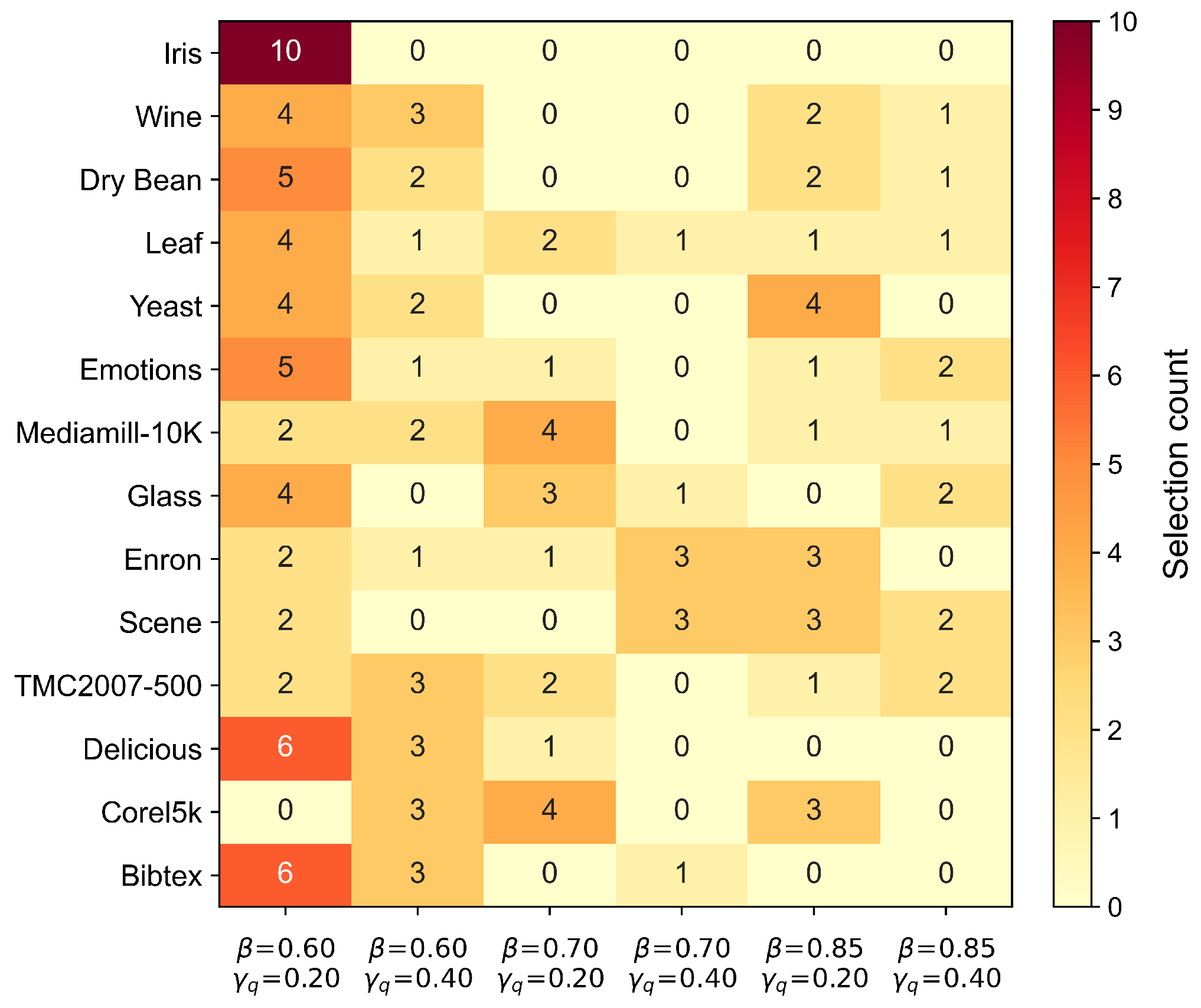
	Nested-d	$\beta =0.6$ (3/5)	${\gamma }_q=0.2$ (4/5)	$\mathrm{k}=20$ (4/5)	5; 20

summarizes the modal parameter choices across the five outer training partitions for each dataset under both protocols, along with the full range of observed k values. Figure 1 aggregates the selected $\beta$–${\gamma }_{\mathrm{quantile}}$ combinations across Equal-d and Nested-d and displays their frequencies for each dataset.

4.2. Main Experimental Results

Table 5. Equal-d results on the five single-label datasets (Macro-F1). Bold underlining = best; italic underlining = second best.

Dataset	Ours	FIMF	VMFS	MFS-MCDM	MCLS	MDFS	SSFS	NRS-Dep
Dry Bean	0.8801	0.8683	0.8745	0.8865	0.8760	0.8490	0.8683	0.8567
Glass	0.4484	0.3721	0.4357	0.3976	0.3971	0.4455	0.3829	0.4348
Iris	0.9831	0.8612	0.9831	0.9831	0.9475	0.9661	0.9323	0.9831
Leaf	0.5644	0.5205	0.5316	0.5406	0.5376	0.4198	0.5174	0.5435
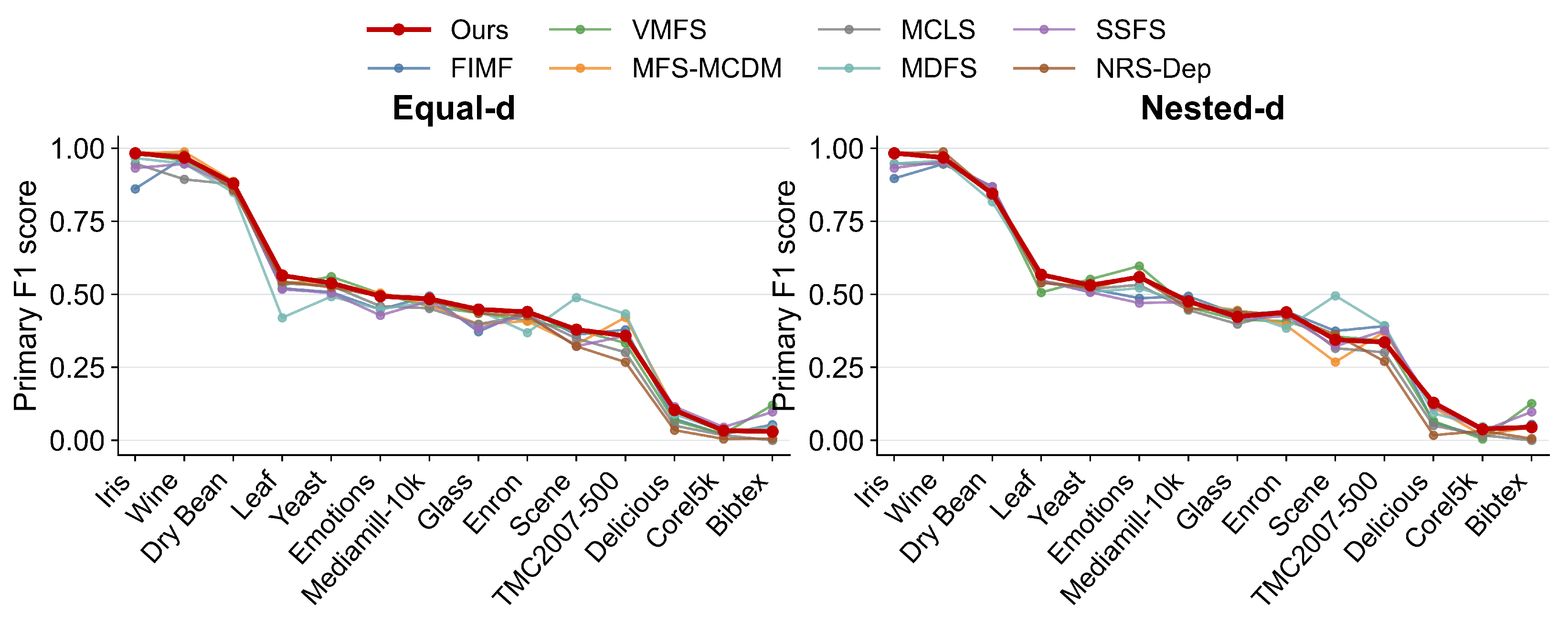
Wine	0.9683	0.9683	0.9571	0.9881	0.8937	0.9474	0.9461	0.9779

and

Table 6. Nested-d results on the five single-label datasets (Macro-F1). Bold underlining = best; italic underlining = second best.

Dataset	Ours	FIMF	VMFS	MFS-MCDM	MCLS	MDFS	SSFS	NRS-Dep
Dry Bean	0.8447	0.8687	0.8468	0.8561	0.8668	0.8174	0.8687	0.8461
Glass	0.4234	0.4314	0.4126	0.4455	0.3980	0.4428	0.4156	0.4420
Iris	0.9831	0.8967	0.9831	0.9831	0.9475	0.9475	0.9323	0.9831
Leaf	0.5672	0.5409	0.5061	0.5706	0.5462	0.5462	0.5473	0.5393
Wine	0.9683	0.9460	0.9683	0.9683	0.9460	0.9571	0.9548	0.9881

report Macro-F1 on the five single-label datasets under Equal-d and Nested-d, respectively;

Table 7. Equal-d results on the nine multi-label datasets (Micro-F1). Bold underlining = best; italic underlining = second best.

Dataset	Ours	FIMF	VMFS	MFS-MCDM	MCLS	MDFS	SSFS	NRS-Dep
Bibtex	0.0299	0.0538	0.1208	0.0350	0.0000	0.0438	0.0971	0.0059
Corel5k	0.0332	0.0202	0.0219	0.0268	0.0172	0.0312	0.0452	0.0049
Delicious	0.1035	0.0733	0.0665	0.1058	0.0505	0.0898	0.1153	0.0346
Emotions	0.4934	0.4481	0.5022	0.5050	0.4595	0.4490	0.4280	0.4934
Enron	0.4396	0.4444	0.4095	0.4077	0.4292	0.3690	0.4290	0.4264
Mediamill-10k	0.4845	0.4943	0.4586	0.4639	0.4519	0.4741	0.4766	0.4784
Scene	0.3791	0.3619	0.3780	0.3281	0.3486	0.4885	0.3222	0.3216
TMC2007-500	0.3579	0.3786	0.3331	0.4211	0.3013	0.4327	0.3575	0.2678
Yeast	0.5383	0.5071	0.5602	0.5364	0.5290	0.4923	0.5042	0.5239

and

Table 8. Nested-d results on the nine multi-label datasets (Micro-F1). Bold underlining = best; italic underlining = second best.

Dataset	Ours	FIMF	VMFS	MFS-MCDM	MCLS	MDFS	SSFS	NRS-Dep
Bibtex	0.0454	0.0552	0.1261	0.0454	0.0000	0.0438	0.0971	0.0059
Corel5k	0.0384	0.0124	0.0045	0.0173	0.0172	0.0473	0.0320	0.0319
Delicious	0.1291	0.0610	0.0658	0.1121	0.0505	0.0927	0.1189	0.0174
Emotions	0.5588	0.4867	0.5965	0.5652	0.5323	0.5210	0.4701	0.5583
Enron	0.4386	0.4415	0.4079	0.3934	0.4408	0.3841	0.4251	0.4282
Mediamill-10k	0.4758	0.4934	0.4559	0.4677	0.4462	0.4681	0.4737	0.4516
Scene	0.3442	0.3744	0.3553	0.2681	0.3152	0.4952	0.3222	0.3622
TMC2007-500	0.3360	0.3910	0.3416	0.3713	0.3013	0.3930	0.3758	0.2704
Yeast	0.5309	0.5187	0.5515	0.5170	0.5179	0.5074	0.5067	0.5239

report Micro-F1 on the nine multi-label datasets. Bold underlining marks the largest score in each dataset row, and italic underlining marks the second-largest score. All scores are means over five outer-test partitions, with parameters and feature counts selected only within the corresponding outer training partition. Figure 2 displays the primary F1 scores across the fourteen evaluation datasets.

4.3. Statistical Significance Test

Table 9. Average ranks under the Equal-d and Nested-d protocols. Values in the table that are bold and underlined indicate the best results; values in italics and underlined indicate the second-best results.

Method	Equal-d Average Rank	Nested-d Average Rank
Ours	2.643	3.429
FIMF	4.786	4.286
VMFS	4.036	4.464
MFS-MCDM	3.464	4.000
MCLS	5.786	5.964
MDFS	4.929	4.500
SSFS	5.179	4.536
NRS-Dep	5.179	4.821

,

Table 10. Friedman test results.

Protocol	Friedman ${\mathit{\chi }}^2$	df	p
Equal-d	17.861	7	0.01261
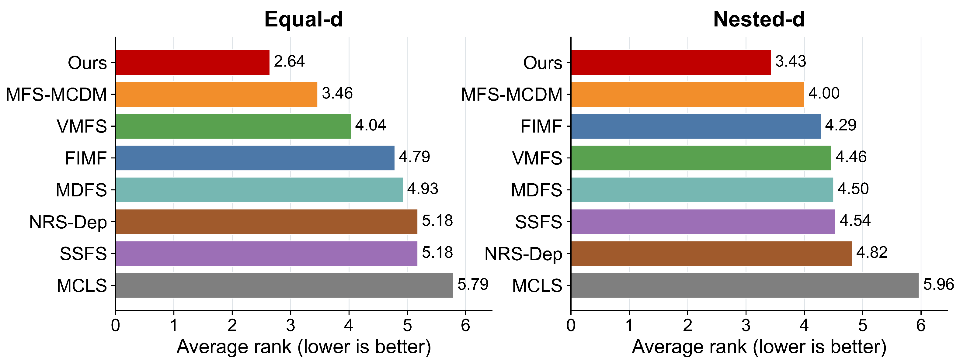
Nested-d	8.761	7	0.2703

and

Table 11. Planned two-sided Wilcoxon signed-rank comparisons with Holm adjustment; $\Delta =\mathrm{Ours}-\mathrm{comparator}$.

Protocol	Comparator	Mean $\Delta$	W/T/L	Raw p	Holm p	Holm $<0.05$
Equal-d	FIMF	0.0237	9/1/4	0.04445	0.2222	No
Equal-d	VMFS	0.0051	10/1/3	0.1025	0.314	No
Equal-d	MFS-MCDM	0.0056	7/1/6	0.4896	0.4896	No
Equal-d	MCLS	0.0332	14/0/0	0.0001221	0.0008545	Yes
Equal-d	MDFS	0.0147	11/0/3	0.1726	0.3452	No
Equal-d	SSFS	0.0201	11/0/3	0.07849	0.314	No
Equal-d	NRS-Dep	0.0251	11/1/2	0.003863	0.02318	Yes
Nested-d	FIMF	0.0118	7/0/7	0.4263	1	No
Nested-d	VMFS	0.0044	6/2/6	0.753	1	No
Nested-d	MFS-MCDM	0.0073	6/3/5	0.5069	1	No
Nested-d	MCLS	0.0256	12/0/2	0.001709	0.01196	Yes
Nested-d	MDFS	0.0015	10/0/4	0.2958	1	No
Nested-d	SSFS	0.0103	11/0/3	0.2412	1	No
Nested-d	NRS-Dep	0.0168	9/1/4	0.1164	0.6982	No

summarize the cross-dataset rank and statistical analyses. Lower average ranks indicate better performance. Figure 3 visually compares the average rank of all methods under both evaluation protocols. Under Equal-d, Ours achieves the lowest average rank ($2.643$), and the Friedman test indicates an overall difference among methods (${\chi }^2=17.861$, p = 0.01261). Holm-adjusted Wilcoxon comparisons are significant for Ours–MCLS (p = 0.000854; $14/0/0$ win/tie/loss) and Ours–NRS-Dep (p = 0.0232; $11/1/2$). Under Nested-d, Ours has an average rank of $3.429$, and the Ours–MCLS comparison is significant after Holm adjustment (p = 0.0120; $12/0/2$).

4.4. Running Time and Scalability

Table 12. Observed resource audit for the full ranking profile; entries are minima–maxima over five outer training partitions.

Dataset	MCBs	Clique Time (s)	Fit Time (s)	Peak Memory (MiB)
Bibtex	55–75	0.00–0.08	0.51–1.18	316–323
Corel5k	52–80	0.00–0.01	0.07–0.18	225–226
Delicious	46–62	0.00–0.01	0.15–0.32	467–469
Dry Bean	112–191	0.00–0.01	0.09–0.40	193–196
Emotions	228–808	0.00–0.02	0.62–3.33	219–238
Enron	50–71	0.00–0.01	0.51–1.05	240–292
Glass	79–174	0.01	0.14–0.18	186–188
Iris	33–40	0.00	0.03	184–185
Leaf	834–2411	0.00–0.14	2.66–22.12	232–383
Mediamill-10k	179–242	0.00–0.01	0.63–7.52	296–322
Scene	254–462	0.00–0.02	1.21–3.76	253–289
TMC2007-500	50–89	0.00–0.01	0.13–0.24	277–280
Wine	91–183	0.00–0.01	0.06–0.20	183–190
Yeast	423–3000	0.01–0.03	3.59–5.39	248–421

summarizes the observed computational range over five outer training partitions.

Across the fourteen datasets, the observed number of maximal consistent blocks ranged from 33–40 on Iris to 834–2411 on Leaf; Yeast spanned 423–3000. Leaf and Yeast showed the widest fold-to-fold ranges and also required longer fitting times than most datasets.

Clique enumeration remained short, with a maximum observed time of 0.14 s, whereas total fitting time ranged from 0.03 s on Iris to 22.12 s on Leaf. The gap between clique time and total fitting time indicates that the subsequent construction of block statistics, discernibility clauses, and inclusion-minimal hitting sets accounts for a substantial part of the computational cost. Peak memory ranged from 183 to 469 MiB, and the largest memory values did not occur on the datasets with the largest numbers of maximal consistent blocks, indicating that memory use depends on the complete fitting pipeline rather than block enumeration alone.

4.5. Metric Settings and Parameter Sensitivity Analysis

All numerical features are standardized using statistics computed from the corresponding training partition, and Euclidean distance is used to construct the tolerance relation for every dataset and outer split. The same metric is retained throughout inner selection and outer evaluation, so $\beta$, ${\gamma }_{\mathrm{quantile}}$, and the feature count are evaluated under a common geometry.

For each outer training partition, the tolerance threshold $\gamma$ is set to the empirical ${\gamma }_{\mathrm{quantile}}$-quantile of its pairwise Euclidean distances. The quantile rule adapts the distance scale to the current training data while preserving the same prespecified construction across datasets. A lower ${\gamma }_{\mathrm{quantile}}$ produces a more local tolerance relation because it selects a smaller quantile of the training-partition distance distribution.

Statistics and labels from the outer test partition are excluded from standardization, threshold construction, parameter selection, and feature count selection. Fixing the distance metric and restricting all data-dependent quantities to the training partition isolates the effects of $\beta$, ${\gamma }_{\mathrm{quantile}}$, and k and keeps the comparison between Equal-d and Nested-d consistent.

Under this configuration, we further examine how the three key parameters are actually selected by the inner-validation procedure across datasets and protocols.

$\beta$ and $\gamma$ are critical parameters that affect the approximation relations of the model, the structure of the maximal consistent blocks, and the final reduction results.

The selected values in Table 4 and Figure 1 are obtained independently within each outer training partition. Across the twenty-eight dataset–protocol settings, ${\gamma }_{\mathrm{quantile}}=0.20$ is the modal choice in twenty-five settings, while the selected $\beta$ values span the complete candidate set. Under Nested-d, the selected feature count varies across outer partitions on thirteen datasets and remains $k=3$ on every Iris partition. The observed frequencies characterize dataset-specific and partition-specific selection under the prespecified inner-validation rule. Because ${\gamma }_{\mathrm{quantile}}=0.20$ is the lower candidate quantile, its predominance corresponds to a more local tolerance relation than ${\gamma }_{\mathrm{quantile}}=0.40$ within the same training partition. These frequencies report inner-validation choices and contain no information from the corresponding outer test partitions.

4.6. Distance Metric Comparison

To verify the rationality of the selected distance metric, this section compares three distance metrics, namely, Euclidean, Manhattan, and cosine, under the same reduction framework.

All three distance metrics are evaluated using $\beta =0.70$ and the quantile parameter ${\gamma }_{\mathrm{quantile}}=0.20$, the same Equal-d feature number, identical five-fold partitions, and the same evaluation population. The distance definition is the sole varying factor; the outer test folds are excluded from configuration decisions.

Table 13. Comparison of different distance metrics.

Dataset	Euclidean	Manhattan	Cosine
Iris	0.9831	0.9831	0.9475
Wine	0.9888	0.9562	0.9563
Glass	0.4164	0.4162	0.4036
Leaf	0.5818	0.5669	0.5535
Dry Bean	0.8904	0.8756	0.8482
Emotions	0.5361	0.5437	0.5542
Scene	0.4346	0.4822	0.4673
Yeast	0.5519	0.4994	0.4973
Enron	0.4473	0.3415	0.4023
Bibtex	0.0299	0.0407	0.0393
Corel5k	0.0283	0.0273	0.0275
Delicious	0.1028	0.1120	0.0996
TMC2007-500	0.3725	0.3426	0.3520
Mediamill-10k	0.4914	0.4840	0.4749

Note: Values are means over five outer test folds. Higher values indicate better performance. Bold underlined and italic underlined values denote the best and second-best results, respectively.

reports Macro-F1 for the single-label datasets and Micro-F1 for the multi-label datasets.

The results demonstrate that no single distance metric achieves optimal performance on all datasets. Euclidean distance obtained the lowest average rank of 1.5357 and achieved the highest or tied-highest mean score on 10 of the 14 datasets. Manhattan and cosine distances obtained average ranks of 2.0357 and 2.4286, with the highest or tied-highest scores on four datasets and one dataset, respectively. Euclidean distance outperformed Manhattan on nine datasets, tied on one, and underperformed on four. It outperformed cosine on 11 datasets and underperformed on three. The lowest average rank and the broadest coverage of best-performing datasets show that Euclidean distance provides the most stable aggregate performance across the evaluated single-label and multi-label datasets. Euclidean distance is therefore adopted as the default setting in the main experiments. This comparison indicates that the distance metric affects the tolerance relation and the structure of the maximal consistent blocks, and the distance form can be further adjusted according to data types in practical applications.

4.7. Ablation Study

The ablation study examines the structural and relevance terms in the ranking profile used by the proposed method. The Full profile combines maximal-block structural evidence, label relevance, the soft-reduct membership contribution, and redundancy control. The structure-removed profile suppresses the maximal-block structural terms and the soft-reduct membership contribution while retaining label relevance and redundancy control. The relevance-removed profile sets the label-relevance contribution to zero while retaining the structural terms, the soft-reduct membership contribution, and redundancy control. The three profiles use identical outer folds, candidate budgets, classifiers, and evaluation metrics. Parameters and feature counts are selected within the corresponding outer training partition for each profile. Macro-F1 is used for the five single-label datasets, and Micro-F1 is used for the nine multi-label datasets.

Table 14. Component ablation on the evaluation datasets. Within each protocol triplet, bold underlining = best; italic underlining = second best.

Dataset	Eq Full	Eq −Struct.	Eq −Rel.	Nest Full	Nest −Struct.	Nest −Rel.
Bibtex	0.0299	0.0407	0.0756	0.0454	0.0507	0.0468
Corel5k	0.0332	0.0275	0.0152	0.0384	0.0235	0.0122
Delicious	0.1035	0.1111	0.0997	0.1291	0.1290	0.1023
Dry Bean	0.8801	0.8588	0.7991	0.8447	0.8757	0.8517
Emotions	0.4934	0.4852	0.4825	0.5588	0.6002	0.5764
Enron	0.4396	0.2787	0.4146	0.4386	0.3247	0.4146
Glass	0.4484	0.4754	0.4079	0.4234	0.4660	0.4195
Iris	0.9831	0.9831	0.8764	0.9831	0.9831	0.9120
Leaf	0.5644	0.5164	0.5177	0.5672	0.5739	0.5677
Mediamill-10k	0.4845	0.4763	0.5041	0.4758	0.4652	0.4958
Scene	0.3791	0.4826	0.4090	0.3442	0.4436	0.4090
TMC2007-500	0.3579	0.3881	0.3714	0.3360	0.4099	0.3371
Wine	0.9683	0.9460	0.9342	0.9683	0.9468	0.9667
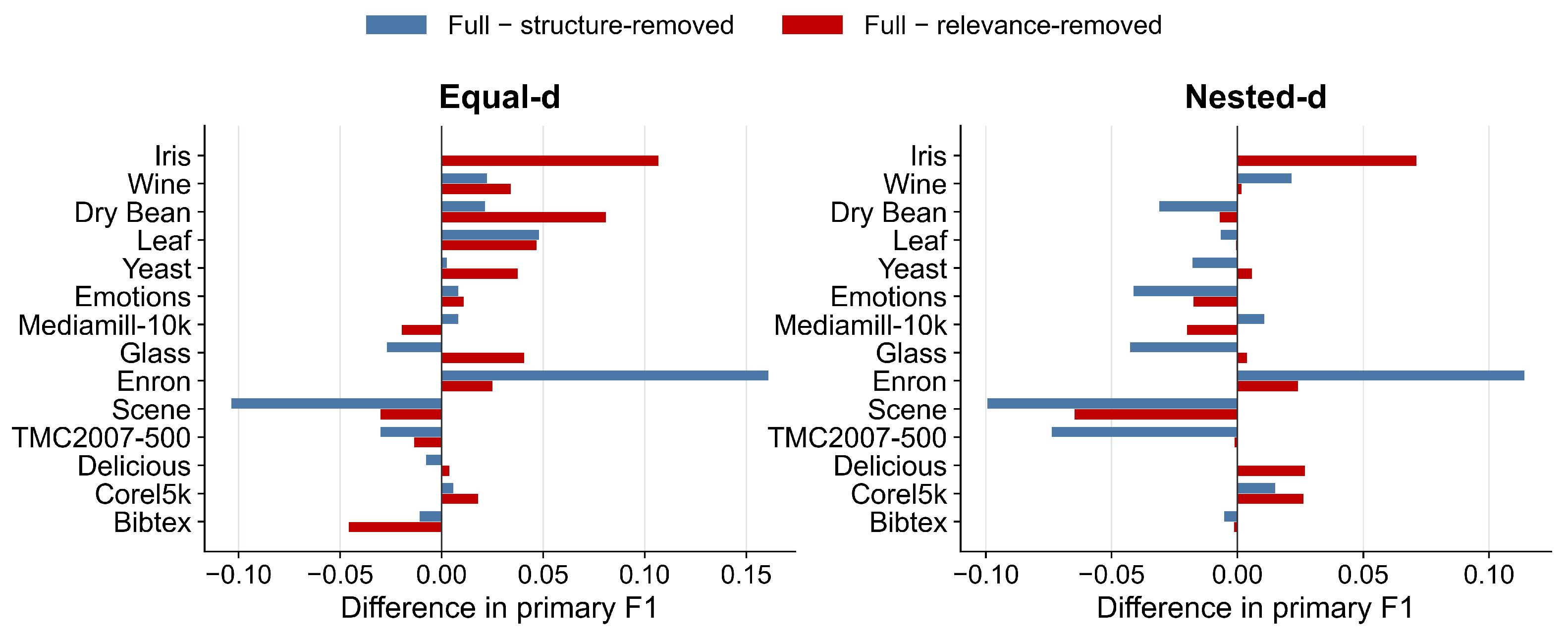
Yeast	0.5383	0.5357	0.5009	0.5309	0.5487	0.5252

reports the primary F1 scores under Equal-d and Nested-d,

Table 15. Paired component contrasts; $\Delta =\mathrm{Full}-\mathrm{ablated}\mathrm{profile}$.

Protocol	Contrast	Mean $\Delta$	W/T/L	Two-Sided p
Equal-d	Full vs. structure-removed	0.0070	8/1/5	0.6602
Equal-d	Full vs. relevance-removed	0.0211	10/0/4	0.104
Nested-d	Full vs. structure-removed	$-0.0112$	5/1/8	0.2856
Nested-d	Full vs. relevance-removed	0.0033	7/0/7	0.583

summarizes the paired dataset-level contrasts, and Figure 4 displays the score differences between the Full profile and each ablated profile.

The component effects vary across datasets. Under Equal-d, the full profile records $8/1/5$ wins/ties/losses against the structure-removed profile and $10/0/4$ against the relevance-removed profile. Under Nested-d, the corresponding counts are $5/1/8$ and $7/0/7$. The positive mean differences for both Equal-d contrasts and for the Nested-d relevance contrast indicate an average benefit from the corresponding complete profile terms within those comparisons. The Nested-d structure contrast varies in the opposite direction on more datasets. These results characterize dataset-dependent contributions of structural evidence and label relevance without implying a universal component effect.

Across the fourteen datasets, Ours obtains the lowest average rank under Equal-d. The Equal-d Friedman test detects an overall method difference, and Holm-adjusted comparisons are significant against MCLS and NRS-Dep. Under Nested-d, the Holm-adjusted comparison with MCLS is significant. The parameter selections in Table 4 are confined to the outer training partitions, and the resource audit reports the observed computational range of maximal-block and inclusion-minimal hitting-set enumeration.

5. Conclusions

Dimensional reduction for continuous single-label and multi-label data is a critical yet challenging task in pattern recognition and machine learning. Targeting the shortcomings of existing rough set-based reduction methods in continuous data processing, this paper proposes a novel dimensional reduction method based on maximal consistent blocks and variable precision rough sets. The proposed method constructs maximal consistent blocks directly from continuous data via distance tolerance relations, avoiding information loss caused by discretization preprocessing. By introducing the variable precision approximation mechanism, the model achieves favorable fault tolerance for noisy samples. Furthermore, unified distribution-based reduction objectives and corresponding discernibility matrix solving algorithms are established for both single-label and multi-label scenarios. Across the fourteen evaluated datasets, Ours attained the lowest average rank under Equal-d, where the Friedman test indicated an overall difference among methods and the Holm-adjusted comparisons with MCLS and NRS-Dep were significant. Under Nested-d, the planned comparison with MCLS remained significant after Holm adjustment. Maximal-block enumeration and inclusion-minimal hitting-set search constitute the output-sensitive stages of the procedure; the resource audit in Section 4.4 reports their observed computational range.

For future work, we will carry out research from four aspects. First, we will extend the current framework to handle continuous multi-label data with missing labels to improve adaptability to real-world incomplete scenarios. Second, we will explore lightweight optimization strategies for the proposed algorithm to further improve computational efficiency for large-scale continuous dimensional reduction tasks. Specifically, since maximal consistent block enumeration is exponential in the worst case, we plan to control its practical cost from three directions: (i) regulating the density of the tolerance graph through the quantile-based distance threshold $\gamma$ so that degenerate dense graphs—which are the main source of the exponential blow-up—are avoided in practice; (ii) adopting pivot-optimized Bron–Kerbosch enumeration with degeneracy ordering, together with pruning and parallelization, so that the enumeration cost remains output-sensitive, i.e., proportional to the number of blocks actually generated rather than to the worst-case bound; and (iii) developing approximate or sampling-based block generation schemes that trade a bounded loss of blocks for substantial speed-ups on massive data. Third, we will extend the model to dynamic incremental continuous multi-label data and develop an incremental dimensional reduction algorithm that avoids full recalculation when samples or features are updated and improves the applicability of the method in dynamic data stream scenarios. In this setting, maximal consistent blocks will be maintained incrementally—only the blocks affected by the updated objects are recomputed and merged—which directly alleviates the enumeration overhead discussed above and provides a natural implementation path for the lightweight strategies in the second aspect. Fourth, we will explore the application of the proposed framework to data preprocessing and feature screening in intelligent systems, such as heterogeneous vehicle platooning and multi-agent collaborative control [51], where high-dimensional continuous monitoring data must be compressed online under strict time and resource budgets. Combining the granularity reduction ability of the proposed rough set method with predefined-time performance constraints and adaptive event-triggered scheduling mechanisms in such systems may further improve the efficiency of downstream decision and control modules, which is worthy of in-depth exploration and verification in follow-up studies.

References

1. Zhou, Z.H.; Zhang, M.L. Multi-label learning. In Encyclopedia of Machine Learning and Data Mining; Springer: New York, NY, USA, 2017; pp. 875–881. [Google Scholar]
2. Liu, Z.; Tang, C.; Abhadiomhen, S.E.; Shen, X.J.; Li, Y. Robust Label and Feature Space Co-Learning for Multi-Label Classification. IEEE Trans. Knowl. Data Eng. 2023, 35, 11846–11859. [Google Scholar] [CrossRef] [Scilit]
3. Ruan, J.; Wang, M.; Liu, D.; Chen, M.; Gao, X. Multi-Label Feature Selection with Feature–Label Subgraph Association and Graph Representation Learning. Entropy 2024, 26, 992. [Google Scholar] [CrossRef] [Scilit] [PubMed]
4. Zhang, J.; Wu, H.; Jiang, M.; Liu, J.; Li, S.; Tang, Y.; Long, J. Group-preserving label-specific feature selection for multi-label learning. Expert Syst. Appl. 2023, 213, 118861. [Google Scholar] [CrossRef] [Scilit]
5. He, Z.; Lin, Y.; Lin, Z.; Wang, C. Multi-label feature selection via similarity constraints with non-negative matrix factorization. Knowl.-Based Syst. 2024, 297, 111948. [Google Scholar] [CrossRef] [Scilit]
6. Li, H.; Fang, M.; Wang, P. Dual dimensionality reduction on instance-level and feature-level for multi-label data. Neural Comput. Appl. 2023, 35, 24773–24782. [Google Scholar] [CrossRef] [Scilit]
7. Hao, P.; Liu, K.; Gao, W. Uncertainty-Aware Global-View Reconstruction for Multi-View Multi-Label Feature Selection. In Proceedings of the AAAI Conference on Artificial Intelligence; AAAI: Palo Alto, CA, USA, 2025; Volume 39, pp. 17068–17076. [Google Scholar]
8. Wan, M.; Cai, M.; Yang, G. Robust exponential graph regularization non-negative matrix factorization technology for feature extraction. Mathematics 2023, 11, 1716. [Google Scholar] [CrossRef] [Scilit]
9. González-López, J.; Ventura, S.; Cano, A. Distributed selection of continuous features in multilabel classification using mutual information. IEEE Trans. Neural Netw. Learn. Syst. 2019, 31, 2280–2293. [Google Scholar] [CrossRef] [Scilit] [PubMed]
10. Yin, T.; Chen, H.; Wan, J.; Zhang, P.; Horng, S.J.; Li, T. Exploiting feature multi-correlations for multilabel feature selection in robust multi-neighborhood fuzzy β covering space. Inf. Fusion 2024, 104, 102150. [Google Scholar] [CrossRef] [Scilit]
11. Ma, J.; Xu, F.; Rong, X. Discriminative multi-label feature selection with adaptive graph diffusion. Pattern Recognit. 2024, 148, 110154. [Google Scholar] [CrossRef] [Scilit]
12. Pawlak, Z. Rough Sets: Theoretical Aspects of Reasoning About Data, 1st ed.; Kluwer Academic Publishers: London, UK, 1991; pp. 1–55. [Google Scholar]
13. Qian, D.; Liu, K.; Wang, J.; Zhang, S.; Yang, X. Attribute reduction based on directional semi-neighborhood rough set. Int. J. Mach. Learn. Cybern. 2025, 16, 2523–2535. [Google Scholar] [CrossRef] [Scilit]
14. Greco, S.; Matarazzo, B.; Slowinski, R. Rough sets theory for multicriteria decision analysis. Eur. J. Oper. Res. 2001, 129, 1–47. [Google Scholar] [CrossRef] [Scilit]
15. Dai, J.; Gao, S.; Zheng, G. Generalized rough set models determined by multiple neighborhoods generated from a similarity relation. Soft Comput. 2018, 22, 2081–2094. [Google Scholar] [CrossRef] [Scilit]
16. Xia, S.; Wang, C.; Wang, G.; Gao, X.; Ding, W.; Yu, J.; Zhai, Y.; Chen, Z. GBRS: A unified granular-ball learning model of pawlak rough set and neighborhood rough set. IEEE Trans. Neural Netw. Learn. Syst. 2023, 36, 1719–1733. [Google Scholar] [CrossRef] [Scilit] [PubMed]
17. Wang, N.; Zhao, E. A new method for feature selection based on weighted k-nearest neighborhood rough set. Expert Syst. Appl. 2024, 238, 122324. [Google Scholar] [CrossRef] [Scilit]
18. Sewwandi, M.A.N.D.; Li, Y.; Zhang, J. Granule-specific feature selection for continuous data classification using neighborhood rough sets. Expert Syst. Appl. 2024, 238, 121765. [Google Scholar] [CrossRef] [Scilit]
19. Zhang, X.; Ou, Q.; Wang, J. Variable precision fuzzy rough sets based on overlap functions with application to tumor classification. Inf. Sci. 2024, 666, 120451. [Google Scholar] [CrossRef] [Scilit]
20. Leung, Y.; Li, D. Maximal consistent block technique for rule acquisition in incomplete information systems. Inf. Sci. 2003, 153, 85–106. [Google Scholar] [CrossRef] [Scilit]
21. Zhang, Z.; Yang, X. Tolerance-based multigranulation rough sets in incomplete systems. Front. Comput. Sci. 2014, 8, 753–762. [Google Scholar] [CrossRef] [Scilit]
22. Li, R.; Chen, H.; Liu, S.; Wang, K.; Wang, B.; Hu, X. TFD-IIS-CRMCB: Telecom fraud detection for incomplete information systems based on correlated relation and maximal consistent block. Entropy 2023, 25, 112. [Google Scholar] [CrossRef] [Scilit] [PubMed]
23. Sun, Y.; Wu, W.Z.; Wang, X. Maximal consistent block based optimal scale selection for incomplete multi-scale information systems. Int. J. Mach. Learn. Cybern. 2023, 14, 1797–1809. [Google Scholar] [CrossRef] [Scilit]
24. Yan, S.; Jusheng, M.; Tao, F.; Leijun, L.; Meishe, L. Maximum consistent block based variable precision rough set model and attribute reduction. J. Front. Comput. Sci. Technol. 2020, 14, 892. [Google Scholar]
25. Leung, Y.; Wu, W.Z.; Zhang, W.X. Knowledge acquisition in incomplete information systems: A rough set approach. Eur. J. Oper. Res. 2006, 168, 164–180. [Google Scholar] [CrossRef] [Scilit]
26. Mroczek, T.; Zheng, R. A new approach to constructing maximal consistent blocks for mining incomplete data. Procedia Comput. Sci. 2022, 207, 1047–1056. [Google Scholar] [CrossRef] [Scilit]
27. Zhang, W.; Qiu, G. Uncertain Decision Making Based on Rough Sets, 1st ed.; Tsinghua University Press: Beijing, China, 2005; pp. 92–93. [Google Scholar]
28. Hu, Q.; Yu, D.; Liu, J.; Wu, C. Neighborhood rough set based heterogeneous feature subset selection. Inf. Sci. 2008, 178, 3577–3594. [Google Scholar] [CrossRef] [Scilit]
29. Mi, J.; Wu, W.Z.; Zhang, W.X. Knowledge reducts based on variable precision rough set theory. Syst. Eng.-Theory Pract. 2004, 24, 116–120. [Google Scholar]
30. Koklu, M.; Ozkan, I.A. Multiclass classification of dry beans using computer vision and machine learning techniques. Comput. Electron. Agric. 2020, 174, 105507. [Google Scholar] [CrossRef] [Scilit]
31. German, B. Glass Identification. 1987. Available online: https://archive.ics.uci.edu/dataset/42/glass+identification (accessed on 20 June 2026).
32. Fisher, R.A. The use of multiple measurements in taxonomic problems. Ann. Eugen. 1936, 7, 179–188. [Google Scholar] [CrossRef] [Scilit]
33. Silva, P.F.B. Development of a System for Automatic Plant Species Recognition. Master’s Thesis, Universidade do Porto (Portugal), Porto, Portugal, 2013. [Google Scholar]
34. Aeberhard, S.; Coomans, D.; De Vel, O. Comparative analysis of statistical pattern recognition methods in high dimensional settings. Pattern Recognit. 1994, 27, 1065–1077. [Google Scholar] [CrossRef] [Scilit]
35. Katakis, I.; Tsoumakas, G.; Vlahavas, I. Multilabel text classification for automated tag suggestion. ECML PKDD Discov. Chall. 2008, 75, 2008. [Google Scholar]
36. Duygulu, P.; Barnard, K.; de Freitas, J.F.; Forsyth, D.A. Object recognition as machine translation: Learning a lexicon for a fixed image vocabulary. In Proceedings of the European Conference on Computer Vision; Springer: Berlin/Heidelberg, Germany, 2002; pp. 97–112. [Google Scholar]
37. Tsoumakas, G.; Katakis, I.; Vlahavas, I. Effective and efficient multilabel classification in domains with large number of labels. In Proceedings of the ECML/PKDD 2008 Workshop on Mining Multidimensional Data (MMD’08); Springer: Berlin/Heidelberg, Germany, 2008; Volume 21, pp. 53–59. [Google Scholar]
38. Trohidis, K.; Tsoumakas, G.; Kalliris, G.; Vlahavas, I. Multi-label classification of music by emotion. EURASIP J. Audio Speech Music Process. 2011, 2011, 4. [Google Scholar] [CrossRef] [Scilit]
39. Klimt, B.; Yang, Y. The enron corpus: A new dataset for email classification research. In Proceedings of the European Conference on Machine Learning; Springer: Berlin/Heidelberg, Germany, 2004; pp. 217–226. [Google Scholar]
40. Snoek, C.G.; Worring, M.; Van Gemert, J.C.; Geusebroek, J.M.; Smeulders, A.W. The challenge problem for automated detection of 101 semantic concepts in multimedia. In Proceedings of the 14th ACM International Conference on Multimedia; ACM: San Jose, CA, USA, 2006; pp. 421–430. [Google Scholar]
41. Boutell, M.R.; Luo, J.; Shen, X.; Brown, C.M. Learning multi-label scene classification. Pattern Recognit. 2004, 37, 1757–1771. [Google Scholar] [CrossRef] [Scilit]
42. Srivastava, A.N.; Zane-Ulman, B. Discovering recurring anomalies in text reports regarding complex space systems. In Proceedings of the 2005 IEEE Aerospace Conference; IEEE: New York, NY, USA, 2005; pp. 3853–3862. [Google Scholar]
43. Elisseeff, A.; Weston, J. A kernel method for multi-labelled classification. Adv. Neural Inf. Process. Syst. 2001, 14, 681–687. [Google Scholar] [CrossRef] [Scilit]
44. Lee, J.; Kim, D.W. Fast multi-label feature selection based on information-theoretic feature ranking. Pattern Recognit. 2015, 48, 2761–2771. [Google Scholar] [CrossRef] [Scilit]
45. Hashemi, A.; Dowlatshahi, M.B.; Nezamabadi-pour, H. VMFS: A VIKOR-based multi-target feature selection. Expert Syst. Appl. 2021, 182, 115224. [Google Scholar] [CrossRef] [Scilit]
46. Hashemi, A.; Dowlatshahi, M.B.; Nezamabadi-pour, H. MFS-MCDM: Multi-label feature selection using multi-criteria decision making. Knowl.-Based Syst. 2020, 206, 106365. [Google Scholar] [CrossRef] [Scilit]
47. Huang, R.; Jiang, W.; Sun, G. Manifold-based constraint Laplacian score for multi-label feature selection. Pattern Recognit. Lett. 2018, 112, 346–352. [Google Scholar] [CrossRef] [Scilit]
48. Zhang, J.; Luo, Z.; Li, C.; Zhou, C.; Li, S. Manifold regularized discriminative feature selection for multi-label learning. Pattern Recognit. 2019, 95, 136–150. [Google Scholar] [CrossRef] [Scilit]
49. Gao, W.; Li, Y.; Hu, L. Multilabel Feature Selection With Constrained Latent Structure Shared Term. IEEE Trans. Neural Netw. Learn. Syst. 2023, 34, 1253–1262. [Google Scholar] [CrossRef] [Scilit] [PubMed]
50. Liu, J.; Lin, Y.; Li, Y.; Weng, W.; Wu, S. Online multi-label streaming feature selection based on neighborhood rough set. Pattern Recognit. 2018, 84, 273–287. [Google Scholar] [CrossRef] [Scilit]
51. Zhao, Y.; Liu, Y.; Zhang, H.; Zhao, N.; Shi, Y. Funnel-based predefined-time output feedback fuzzy adaptive event-triggered platoon control for heterogeneous vehicles. IEEE Internet Things J. 2026, early access. [Google Scholar] [CrossRef] [Scilit]
Figure 1. Frequency of β and γ quantile selections within the outer training partitions.
Mathematics 14 03000 g001
Figure 2. Primary F1 scores across the fourteen evaluation datasets. Macro-F1 is shown for the five single-label datasets and Micro-F1 for the nine multi-label datasets.
Mathematics 14 03000 g002
Figure 3. Average ranks across the fourteen evaluation datasets under the Equal-d and Nested-d protocols.
Mathematics 14 03000 g003
Figure 4. Component-ablation score differences across the evaluated datasets.
Mathematics 14 03000 g004