Fixed-Time Quasi-Consensus and Quasi-Containment Control for Multi-Agent Systems Under Non-Periodic Unknown DoS Attacks

Abstract

This study investigates the fixed-time quasi-consensus and quasi-containment control for multi-agent systems (MASs) under non-periodic unknown denial-of-service (DoS) attacks. Most available strategies fail to construct fixed-time observers and feasible corresponding parameter tuning rules to guarantee the precise fixed-time convergence of observer states to the convex hull trajectory spanned with multiple leaders under arbitrary non-periodic DoS interference. Moreover, most existing relevant fixed-time cooperative control methods for MASs commonly impose restrictive assumptions on system input matrices, requiring the matrix to be square and invertible, which severely limits their practical applicability. To overcome these limitations, the observers and corresponding parameter selection conditions are designed in this study, which can ensure that the observer states converge to the target trajectory formed by the leaders within a fixed time under non-periodic unknown DoS attacks. Then, based on the linear transformation of the state space and the theory of sliding mode control, a novel observer-based controller is proposed to solve the fixed-time quasi-consensus and quasi-containment control problems. The proposed approach remains effective even when, under mild conditions, the input matrix is non-square or non-invertible—a challenge that many existing methods cannot address. Finally, numerical simulations demonstrate that the proposed control strategy enables MASs with non-square input matrices suffering from unknown non-periodic DoS attacks to achieve fixed-time quasi-consensus and quasi-containment under mild conditions.

1. Introduction

With the rapid development of scientific and technological means, the cooperative control of multi-agent systems (MASs) has become a popular research topic, which can be largely attributed to its broad utilization scenarios ranging from vehicle formation and intelligent robots to spacecraft systems [1,2,3]. In the literature, the consensus and containment control issues (an extension of consensus) are the most fundamental and important topics on the cooperative control of MASs. At present, numerous scholars have conducted research on these two types of issues and provided effective methods. In [4], the consensus problem of single-integrator MASs was investigated. The Laplacian matrix was adopted to derive a sufficient consensus condition, which laid a foundation for the research on consensus and containment control. After that, these problems for more complex and realistic MASs have been extensively investigated. In [5], the consensus issue of second-order MASs with external disturbance was studied. Reference [6] conducted research on containment control applicable to general linear MASs, alongside developing a corresponding distributed control strategy. For the scenario where individual agents in MASs have heterogeneous dynamics, refs. [7,8,9] investigated heterogeneous MASs and provided the control protocols based on dynamic compensators. Moreover, the consensus of nonlinear MASs was considered in [10,11].

Most early relevant studies, as presented in [4,5,6,7,8,9,10,11], only investigated control schemes for MASs under ideal communication environments, wherein the systems—and particularly their communication networks—are assumed to be free from attacks. However, actual MASs usually rely on open communication networks for information exchange, which poses severe cybersecurity threats to them. Among all types of cyber attacks, denial-of-service (DoS) attacks can effectively disrupt inter-agent data exchange by jamming communication channels, thereby degrading collaborative performance or even causing system instability. Therefore, designing control strategies that ensure effective control of MASs under DoS attacks is of paramount importance. In [12], the consensus issue of MASs under fixed periodic DoS attacks was investigated. Combined with event/self-triggered mechanism, the control method solving the secure consensus issue of MASs under DoS attacks was designed in [13]. In [14], the dynamic event-triggered control scheme was investigated for heterogeneous MASs under DoS attacks. Reference [15] carried out research on consensus control targeting linear MASs subject to stochastic DoS attacks, whereas a similar question is discussed for nonlinear MASs within [16]. Moreover, the observer-based event-triggered control schemes for nonlinear system and heterogeneous MASs under DoS attacks were investigated in [17] and [18], respectively. In [19], the event-based control approach for MASs considering non-periodic DoS attacks was designed. In [20], the hidden Markov process was used to characterize the behavior of DoS attacks and a scheme combining consensus control and fault detection was designed. Furthermore, the generalized dynamic observers for discrete Markovian cyber-physical systems was designed in [21].

A shared characteristic of most aforementioned results is that MASs can only achieve asymptotic convergence to the desired targets under the designed control protocols. Nevertheless, to enhance the convergence speed and efficiency of MASs under resource-constrained or poor network conditions, achieving convergence in finite time better satisfies practical engineering demands. Therefore, designing control strategies that allow MASs to attain control goals in finite time is of higher research value. In [22], a control scheme that enables uncertain MASs to achieve consensus within a finite time was provided, and a similar issue based on the event-triggered mechanism was considered in [23]. Despite these strategies realizing finite-time consensus, their settling time is relevant to the initial states of systems. In other words, if the initial conditions are unknown, the settling time cannot be predicted. To address this issue, research on designing control schemes that ensure fixed-time convergence under arbitrary initial conditions has become particularly important. The research in [24] explored fixed-time coordination problems for uncertain MASs under both continuous and intermittent control frameworks. The fixed-time control strategies for linear and nonlinear MASs were investigated in [25] and [26], respectively. In [27,28,29], the design of event-based control strategies that enable MASs to realize fixed-time consensus was considered. Aiming at MASs suffering from DoS attacks, the control strategies resolving consensus and containment control issues were explored in [30,31] and [32], respectively. In addition, benefiting from the inherent capability of sliding mode control (SMC) to drive system states to the predefined sliding surface within a finite time, considerable efforts have been devoted to designing SMC-based protocols to realize fixed-time control. For example, in [33], the fixed-time observer based on SMC was designed for photovoltaic systems, and the robust control scheme based on SMC was considered in [34]. However, owing to inherent flaws of SMC, such as severe chattering, reliance on continuous full-state and neighbor information, vulnerability to DoS attacks-induced random communication delays, and packet losses and tedious parameter tuning for coupled MASs, SMC is rarely directly deployed in DoS-attacked MASs.

Although abundant achievements have been acquired regarding the fixed-time consensus and containment control of MASs, several limitations in this study cannot be ignored:

• Since the disruption of inter-agent communication by DoS attacks poses a fundamental challenge to MAS control, most existing countermeasures rely on idealized assumptions about the attacks. For example, the precise time-domain profile of DoS attacks is presumed to be fully accessible in [35], whereas known attack moments and fixed periodic attack patterns are required in [12,32]. Nevertheless, non-periodic, random, and completely unknown attack patterns are exhibited by practical DoS interference in real engineering scenarios. Failures of the above-mentioned control frameworks can be easily triggered under such unstructured unknown attacks, since the corresponding theoretical derivations and convergence guarantees are established upon over-simplified attack models.
• To achieve fixed-time convergence, most existing studies impose stringent requirements on the system input, specifically on the input matrix within the system model. For example, nonlinear MASs models were studied in [26,27,31,36], yet an identity input matrix was mandated in these studies. Moreover, while refs. [28,37] removed this identity matrix restriction, but another constraint was introduced—the input matrix must be square and invertible. This constraint is essentially equivalent to the identity matrix assumption, as one can be transformed into the other via a state transformation. Consequently, these restrictions exclude many underactuated systems, where the number of input channels is lower than the state dimension (i.e., the input matrix is non-square), thereby limiting the generality of the theoretical results.

Ultimately, this study aimed to address these limitations.

This study investigates the fixed-time quasi-consensus and quasi-containment control issues for MASs under non-periodic unknown DoS attacks. The main contributions are listed as follows:

• Fixed-time observers are developed to handle consensus and containment control issues, respectively. Distinct from the prior resilient general and observer-based control schemes reported in [12,17,18,21,32,33,34,35], where either only consider periodic and known DoS attack models or merely guarantee effective control without fixed-time convergence guarantees, the presented observers can precisely recover leader states for consensus tasks and composite leader-generated target trajectories for containment control within a fixed settling time. Such favorable performance can be guaranteed even under non-periodic, unknown DoS attacks that break the connectivity of communication topologies, which enables stable supply of reliable leader state signals to the subsequent control protocol.
• Based on a linear transformation of the state space and the theory of sliding mode control, a novel controller is provided. Compared with the control schemes presented in [26,27,28,31,36,37], where either identity input matrices or square invertible input matrices are mandated as indispensable prerequisites, the developed controller achieves fixed-time quasi-consensus and quasi-containment control of MASs while greatly loosening the structural restrictions on the input matrix. Favorable fixed-time control performance can be guaranteed even when the input matrix is non-square and non-invertible under mild admissible conditions. Such a breakthrough substantially expands the applicable scope of the control framework to a class of underactuated systems, and remarkably improves the generality and practical value of the derived theoretical conclusions.

The organization of the remainder of this study is outlined below: The preliminaries and problem formulation are given in Section 2 and Section 3, respectively. In Section 4 and Section 5, the design protocols of the observer and the controller are provided, respectively. Numerical examples are demonstrated in Section 6. In Section 7, the conclusion is given.

2. Preliminaries

2.1. Notations

${\mathbf{R}}^{n\times m}$ and ${\mathbf{R}}^m$ stand for the sets of $n\times m$-dimensional real matrices and m-dimensional Euclidean space, respectively. For any matrix X, $\mathbf{rank}(X)$ represents the rank of X. $\parallel ·\parallel$ represents the Euclidean norm of vectors or matrices’ 2-norm. For any $x={[x_1,x_2,\dots ,x_n]}^T\in {\mathbf{R}}^n$ and $r>0$, ${\lceil x\rfloor }^r=[|x_1{|}^r\mathrm{sign}(x_1),|x_2{|}^r\mathrm{sign}(x_2),\dots ,|x_n{{|}^r\mathrm{sign}(x_n)]}^T$, where $\mathrm{sign}(·)$ represents the signal function. A matrix $Q\in {\mathbf{R}}^{n\times n}$ is considered symmetric positive definite, denoted by $Q>0$, if $Q^T=Q$ and all its eigenvalues are positive. ${\lambda }_{\min }(Q)$ represents the minimum eigenvalue of Q. ${\mathbf{0}}_{m\times n}$ stands for a $m\times n$-dimensional zero matrix, and $I_n$ is the $n\times n$-dimensional identity matrix. For any $y>0$, $\lceil y\rceil =\inf \{y^{\ast }|y^{\ast }\in \mathbf{Z},y^{\ast }\ge y\}$ ($\mathbf{Z}$ represents the set of integers).

2.2. Topology Graph

Consider MASs with $N+M$ agents, including N followers (the first N agents) and M leaders (the remaining M agents), the index sets for followers and leaders are denoted as $\mathcal{F}=\{1,2,\dots ,N\}$ and $\mathcal{L}=\{N+1,N+2,\dots ,N+M\}$, respectively. The information interaction relationships among all agents are characterized by the topology matrix $\mathcal{A}=\{a_{ij}\}\in {\mathbf{R}}^{(N+M)\times (N+M)}$, where the matrix element $a_{ij}$ is positive if agent i can obtain direct information from agent j, and zero otherwise. For a sequence of agent indices $s_w$$(w=1,2,\dots ,m,s_w\in \{1,2,\dots ,N+M\})$, if the matrix elements $a_{s_1{s}_2},a_{s_2{s}_3},\dots ,a_{s_{m-1}{s}_m}0$ are all positive, the set of these elements forms a directed information path enabling agent $s_1$ to obtain message from agent $s_m$. Define $H=h_{ij}\in {\mathbf{R}}^{(N+M)\times (N+M)}$ as a Laplacian matrix, where $h_{ij}$ represents the $(i,j)$-th element of H such that $h_{ij}={\sum }_{k=1}^{N+M}{a}_{ik}$ if $i=j$ and $h_{ij}=-a_{ij}$ otherwise. In this study, leaders cannot receive information from any agent and $a_{ii}\equiv 0$ holds for all $i=1,2,\dots ,N+M$. Hence, H can be given as follows:

$$\begin{array}{c}\hfill H=\left(\begin{array}{cc}{H}_1& H_2\\ \mathbf{0}& \mathbf{0}\end{array}\right),\end{array}$$

where $H_1\in {\mathbf{R}}^{N\times N}$ and $H_2\in {\mathbf{R}}^{N\times M}$. This study imposes the following assumption on the Laplacian matrix H.

Assumption 1

([38]). Every follower is reachable from at least one leader through a directed path, whereas leaders cannot receive information via any path originating from other agents. The communication graph restricted to followers is undirected, satisfying $a_{ij}=a_{ji}$ for any $i,j\in \mathcal{F}$.

Hence, the following conclusion is true.

Lemma 1

([38]). When Assumption 1 holds, $H_1>0$. Moreover, all entries of $-H_1^{-1}{H}_2$ are non-negative, and each row sum of $-H_1^{-1}{H}_2$ equals 1.

2.3. DoS Attacks

This study considers MASs under unknown connectivity-destructive DoS attacks. Specifically, the time-varying Laplacian matrix $H(t)$ is unavailable a priori. The network topology connectivity corresponding to $H(t)$ will be destroyed during the time intervals belonging to $T_{\mathrm{under}}$, while $H(t)$ degenerates to the fixed matrix H for $t\in T_{\mathrm{without}}$. Here, $H(t)$ denotes the real-time Laplacian matrix of the MASs at time t, $T_{\mathrm{under}}$ is the time set where the MASs suffer from DoS attacks, and $T_{\mathrm{without}}$ represents the attack-free time set. The next assumption of DoS attacks is held in this study.

Assumption 2.

There exist constants $T>0$, $0<\rho <1$, and $0<\tau <\rho T$ such that the following statements hold for every time window $[rT,(r+1)T)$, $r=0,1,2,\dots$:

1. 

The window $[rT,(r+1)T)$ can be partitioned into finitely many left-closed and right-open subintervals, where each subinterval corresponds to a single communication status: either fully attacked or fully attack-free without status switching inside any subinterval;

2. 

The total length of all attack-free subintervals within $[rT,(r+1)T)$ is no less than $\rho T$;

3. 

Every individual attack-free subinterval contained in $[rT,(r+1)T)$ has a duration no less than τ.

Remark 1.

According to Assumption 2, the DoS attacks considered in this study are aperiodic. Specifically, although a fixed interval T is assumed, the actual attack timings within each interval of length T are entirely random. Only the minimum proportion ρ of attack-free time and the minimum duration τ of each attack-free period are specified, which are necessary for system analysis. Therefore, compared with the existing literature such as [12,32,35], the DoS attack model examined in this study is more general.

2.4. Basic Lemmas

The following Lemmas are used in this study.

Lemma 2

([39]). If $w_i\ge 0$ for $i\in \{1,2,\dots ,s\}$, next two results hold.

$$\begin{array}{c}\hfill {\displaystyle \sum _{i=1}^s}{w}_i^g\ge ({\displaystyle \sum _{i=1}^s}{w}_i{)}^g,0<g<1,\\ \hfill {\displaystyle \sum _{i=1}^s}{w}_i^g\ge s^{1-g}({\displaystyle \sum _{i=1}^s}{w}_i{)}^g,g>1.\end{array}$$

Lemma 3

([24]). Consider real-valued function $V(t)$ with $V(0)\ge 0$ and

$$\begin{array}{c}\hfill \dot{V}(t)=-a_1{V}^{b_1}(t)-a_2{V}^{b_2}(t),\end{array}$$

where $a_1,a_2>0$, $0<b_1<1$ and $b_2>1$. In this case, $V(t)=0$ for any $t\ge T_{\max }$, where $T_{\max }={\displaystyle \frac{1}{a_1(1-b_1)}}+{\displaystyle \frac{1}{a_2(b_2-1)}}$.

3. Problem Formulation

Consider the MASs given as follows:

$$\begin{array}{c}\hfill {\dot{x}}_i(t)=\left\{\begin{array}{cc}A{x}_i(t)+B{u}_i(t),\hfill & i\in \mathcal{F},\hfill \\ A{x}_i(t),\hfill & i\in \mathcal{L}.\hfill \end{array}\right.\end{array}$$

(1)

where $x_i(t)\in {\mathbf{R}}^n$ represents the state of agent i, $u_i(t)\in {\mathbf{R}}^m$ represents the input of follower i, $m\le n$. $A\in {\mathbf{R}}^{n\times n}$ and $B\in {\mathbf{R}}^{n\times m}$ are the system and input matrices, respectively. The next assumption about A and B holds in this study.

Assumption 3.  (i) $\mathit{rank}(B)=m$; (ii) $2m\ge n$; (iii) there exist nonsingular matrices ${\Gamma }_1\in {\mathit{R}}^{n\times n}$ and ${\Gamma }_2\in {\mathit{R}}^{m\times m}$ such that

$$\begin{array}{cc}\hfill {\Gamma }_1^{-1}A{\Gamma }_1=& \left[\begin{array}{cc}{\alpha }_1& {\alpha }_2\\ {\mathbf{0}}_{(n-m)\times m}& I_{n-m}\\ {\beta }_1& {\beta }_2\end{array}\right],\hfill \end{array}$$

(2)

$$\begin{array}{cc}\hfill {\Gamma }_1^{-1}B{\Gamma }_2=& \left[\begin{array}{cc}{I}_{2m-n}& {\mathbf{0}}_{(2m-n)\times (n-m)}\\ {\mathbf{0}}_{(n-m)\times (2m-n)}& {\mathbf{0}}_{(n-m)\times (n-m)}\\ {\mathbf{0}}_{(n-m)\times (2m-n)}& I_{n-m}\end{array}\right],\hfill \end{array}$$

(3)

where

$$\begin{array}{cc}\hfill {\alpha }_1& =\left[\begin{array}{ccc}{\alpha }_{1,1}& \dots & {\alpha }_{1,m}\\ ⋮& \ddots & ⋮\\ {\alpha }_{2m-n,1}& \dots & {\alpha }_{2m-n,m}\end{array}\right],\hfill \\ \hfill {\alpha }_2& =\left[\begin{array}{ccc}{\alpha }_{1,m+1}& \dots & {\alpha }_{1,n}\\ ⋮& \ddots & ⋮\\ {\alpha }_{2m-n,m+1}& \dots & {\alpha }_{2m-n,n}\end{array}\right],\hfill \\ \hfill {\beta }_1& =\left[\begin{array}{ccc}{\beta }_{m+1,1}& \dots & {\beta }_{m+1,m}\\ ⋮& \ddots & ⋮\\ {\beta }_{n,1}& \dots & {\beta }_{n,m}\end{array}\right],\hfill \\ \hfill {\beta }_2& =\left[\begin{array}{ccc}{\beta }_{m+1,m+1}& \dots & {\beta }_{m+1,n}\\ ⋮& \ddots & ⋮\\ {\beta }_{n,m+1}& \dots & {\beta }_{n,n}\end{array}\right].\hfill \end{array}$$

Remark 2.

Set $Q_c=[b_{(1)},b_{(2)},\dots ,b_{(2m-n)},b_{(2m-n+1)},A{b}_{(2m-n+1)},b_{(2m-n+2)},A{b}_{(2m-n+2)}$, $\dots ,b_{(m)},A{b}_{(m)}]$, where $\{b_{(1)},b_{(2)},\dots ,b_{(m)}\}$ denotes a permutation of all column vectors of B, rather than the original ordered columns of B. If Assumption 3 is held and $Q_c$ is full-rank, the matrices ${\Gamma }_1$ and ${\Gamma }_2$ can be constructed as follows. First, build a preliminary state transformation matrix ${\widehat{\Gamma }}_1=[e_1,e_2,\dots ,e_{2m-n},e_{2m-n+1,1},e_{2m-n+1,2},\dots ,e_{m,1},e_{m,2}]$, where $e_i=b_{(i)}$, $e_{j,1}=A{b}_{(j)}+{\alpha }_{j,1}{b}_{(j)}$, $e_{j,2}=b_{(j)}$ for $i=1,2,\dots ,2m-n$, $j=2m-n+1,2m-n+2,\dots ,m$. ${\alpha }_{j,1}$ is the solution of $-A^2{b}_{(j)}=A{\alpha }_{j,1}{b}_{(j)}+{\alpha }_{j,0}{b}_{(j)}$. According to the classical Wonham controllable canonical form theory [40], the transformation ${\widehat{\Gamma }}_1$ can convert $(A,B)$ into the standard multi-input controllable canonical form, such that ${\widehat{\Gamma }}_1^{-1}A{\widehat{\Gamma }}_1$ and ${\widehat{\Gamma }}_1^{-1}B$ exhibit the standard structural features for systems with controllability indices 1 and 2. Based on this standard canonical form, simple invertible row and column permutations, as well as input scaling operations, are further performed to yield the customized block structure in (2) and (3). The resulting ${\Gamma }_1$ and ${\Gamma }_2$ are nonsingular and satisfy all the requirements in Assumption 3.

Based on the above analysis, a method for effectively calculating ${\Gamma }_1$ and ${\Gamma }_2$ has been obtained, which can be used to determine whether the condition $\mathrm{rank}\left[B,AB\right]=n$ holds. If this condition is satisfied, the matrix $Q_c$ is full rank and the standard construction method of the Wonham controllable canonical form can be used to calculate ${\Gamma }_1$ and ${\Gamma }_2$.

Consider the situation that $M=1$, the definition of fixed-time quasi-consensus of MASs is given as follows.

Definition 1

([32]). The fixed-time quasi-consensus problem of MASs (1) is solved if there exist positive constants $T_{\max }$ and δ such that ${\sum }_{i=1}^N\parallel x_i(t)-x_0(t)\parallel \le \delta$ for any $t\ge T_{\max }$ and $x_i(0),x_0(0)\in {\mathit{R}}^n$, where $x_0(t)$ represents the state of single leader.

Consider the situation that $M\ge 2$, the basic definitions and lemma about fixed-time quasi-containment control of MASs are given as follows.

Definition 2

([41]). Consider a set $\mathcal{C}$ defined on the real vector space $V\subseteq {\mathit{R}}^n$. The set $\mathcal{C}$ is called a convex set if for arbitrary $x,y\in \mathcal{C}$ and any $z\in [0,1]$, the convex combination $zx+(1-z)y\in \mathcal{C}$ still belongs to $\mathcal{C}$. For a point set $X=\{x_1,x_2,\dots ,x_m\}$ in V, its convex hull is defined as the smallest convex that incorporates all elements of X. In this study, $\mathit{Co}\{X\}$ is adopted to represent the convex hull of the set X. Equivalently, the mathematical expression of $\mathit{Co}\{X\}$ is given as follows:

$$\begin{array}{c}\hfill \mathit{Co}\{X\}=\left\{{\displaystyle \sum _{i=1}^m}{\alpha }_i{x}_i|x_i\in X,{\alpha }_i\ge 0,{\displaystyle \sum _{i=1}^m}{\alpha }_i=1\right\}.\end{array}$$

Based on Lemma 1 and Definition 2, the next conclusion can be given.

Lemma 4

([42]). Define $\psi (t)=x_{\mathcal{F}}(t)+(H_1^{-1}{H}_2\otimes I_n)x_{\mathcal{L}}(t)$, where $x_{\mathcal{F}}(t)={[x_1^T(t),x_2^T(t),\dots ,x_N^T(t)]}^T$ and $x_{\mathcal{L}}(t)={[x_{N+1}^T(t),x_{N+2}^T(t),\dots ,x_{N+M}^T(t)]}^T$. It follows that $x_i(t)\in \mathit{Co}\{X(t)\}$ for any $i\in \mathcal{F}$ if Assumption 1 is satisfied and $\parallel \psi (t)\parallel =0$, where $X(t)=\{x_{N+1}(t),x_{N+2}(t),\dots ,x_{N+M}(t)\}$.

Based on Lemma 4, the definition of fixed-time quasi-containment control is given as follows.

Definition 3

([43]). The fixed-time quasi-containment control problem of MASs (1) is solved if there exist positive constants $T_{\max }$ and δ such that $\parallel \psi (t)\parallel \le \delta$ for any $t\ge T_{\max }$ and $x_i(0)\in {\mathit{R}}^n$.

The main objective of this study is to design proper control schemes making MASs (1) solve fixed-time quasi-consensus problem (when $M=1$) and fixed-time quasi-containment control problem (when $M\ge 2$).

4. Design of Observer

4.1. Observer for Quasi-Consensus Problem

4.1.1. Without DoS Attacks

For MASs (1) without DoS attacks and with $M=1$, the observer for each follower is given as follows:

$$\begin{array}{cc}\hfill {\dot{\widehat{x}}}_i(t)& =A{\widehat{x}}_i(t)-{\widehat{\kappa }}_1{\lceil {\widehat{\epsilon }}_i(t)\rfloor }^{{\widehat{r}}_1}-{\widehat{\kappa }}_2{\lceil {\widehat{\epsilon }}_i(t)\rfloor }^{{\widehat{r}}_2}-{\widehat{\kappa }}_3{\widehat{\epsilon }}_i(t),i\in \mathcal{F},\hfill \end{array}$$

(4)

where ${\widehat{\epsilon }}_i(t)={\sum }_{j=1}^N{a}_{ij}({\widehat{x}}_i(t)-{\widehat{x}}_j(t))+b_i({\widehat{x}}_i(t)-x_0(t))$, $b_i=a_{iN+1}$. $0<{\widehat{r}}_1<1$ and ${\widehat{r}}_2>1$. ${\widehat{\kappa }}_1$, ${\widehat{\kappa }}_2$ and ${\widehat{\kappa }}_3$ need to be calculated.

Then, the following conclusion can be obtained.

Proposition 1.

Assume that Assumption 1 is held, if ${\widehat{\kappa }}_1$, ${\widehat{\kappa }}_2$, and ${\widehat{\kappa }}_3$ satisfy the following conditions:

$$\begin{array}{cc}\hfill & {\widehat{\kappa }}_1>0,\hfill \end{array}$$

(5)

$$\begin{array}{cc}\hfill & {\widehat{\kappa }}_2>0,\hfill \end{array}$$

(6)

$$\begin{array}{cc}\hfill & {\widehat{\kappa }}_3>{\displaystyle \frac{\parallel A\parallel }{{\lambda }_{\min }(H_1)}},\hfill \end{array}$$

(7)

then $\parallel {\widehat{x}}_i(t)-x_0(t)\parallel =0$ for any $t\ge T_{\max }^1$, where

$$\begin{array}{cc}\hfill T_{\max }^1& ={\displaystyle \frac{1}{{\widehat{p}}_1(1-{\widehat{r}}_1)}}+{\displaystyle \frac{1}{{\widehat{p}}_2({\widehat{r}}_2-1)}},\hfill \\ \hfill {\widehat{p}}_1& ={\widehat{\kappa }}_1{({\lambda }_{\min }(H_1))}^{{\displaystyle \frac{{\widehat{r}}_1+1}{2}}},\hfill \\ \hfill {\widehat{p}}_2& ={\widehat{\kappa }}_2{({\lambda }_{\min }(H_1))}^{{\displaystyle \frac{{\widehat{r}}_2+1}{2}}}{(Nn)}^{-{\displaystyle \frac{{\widehat{r}}_2-1}{2}}}.\hfill \end{array}$$

Proof of Proposition 1.

Set ${\widehat{e}}_i(t)={\widehat{x}}_i(t)-x_0(t)$ and $\widehat{e}(t)={[{\widehat{e}}_1^T(t),{\widehat{e}}_2^T(t),\dots ,{\widehat{e}}_N^T(t)]}^T$; then, we have $\parallel {\widehat{x}}_i(t)-x_0(t)\parallel =0$ if $\parallel \widehat{e}(t)\parallel =0$ and

$$\begin{array}{cc}\hfill \dot{\widehat{e}}(t)& =(I_N\otimes A)\widehat{e}(t)-{\widehat{\kappa }}_1{\lceil \widehat{\epsilon }(t)\rfloor }^{{\widehat{r}}_1}-{\widehat{\kappa }}_2{\lceil \widehat{\epsilon }(t)\rfloor }^{{\widehat{r}}_2}-{\widehat{\kappa }}_3\widehat{\epsilon }(t),\hfill \end{array}$$

(8)

where $\widehat{\epsilon }(t)={[{\widehat{\epsilon }}_1^T(t),{\widehat{\epsilon }}_2^T(t),\dots ,{\widehat{\epsilon }}_N^T(t)]}^T$.

Set $\widehat{V}(t)={\widehat{e}}^T(t)(H_1\otimes I_n)\widehat{e}(t)$ as the Lyapunov function; then, we have

$$\begin{array}{cc}\hfill \dot{\widehat{V}}(t)& ={\widehat{e}}^T(t)(H_1\otimes (A+A^T))\widehat{e}(t)-2{\widehat{\kappa }}_1{\widehat{\epsilon }}^T(t){\lceil \widehat{\epsilon }(t)\rfloor }^{{\widehat{r}}_1}-2{\widehat{\kappa }}_2{\widehat{\epsilon }}^T(t){\lceil \widehat{\epsilon }(t)\rfloor }^{{\widehat{r}}_2}-2{\widehat{\kappa }}_3{\widehat{\epsilon }}^T(t)\widehat{\epsilon }(t).\hfill \end{array}$$

(9)

It can be obtained that ${\widehat{e}}^T(t)(H_1\otimes (A+A^T))\widehat{e}(t)\le 2\parallel A\parallel \widehat{V}(t)$. Meanwhile, based on Lemma 1, ${\widehat{\kappa }}_3{\widehat{\epsilon }}^T(t)\widehat{\epsilon }(t)\ge {\lambda }_{\min }(H)\widehat{V}(t)$. Moreover, since $0<{\widehat{r}}_1<1$ and ${\widehat{r}}_2>1$, we have $0<{\displaystyle \frac{1+{\widehat{r}}_1}{2}}<1$ and ${\displaystyle \frac{1+{\widehat{r}}_2}{2}}>1$. Define ${\widehat{\epsilon }}_{ij}(t)$ as the j-th element of ${\widehat{\epsilon }}_i(t)$ for $i\in \{1,2,\dots ,N\}$ and $j\in \{1,2,\dots ,n\}$, based on Lemma 2,

$$\begin{array}{cc}\hfill {\widehat{\epsilon }}^T(t){\lceil \widehat{\epsilon }(t)\rfloor }^{{\widehat{r}}_1}& ={\displaystyle \sum _{i=1}^N}{\displaystyle \sum _{j=1}^n}(|{\widehat{\epsilon }}_{ij}(t){{|}^2)}^{{\displaystyle \frac{1+{\widehat{r}}_1}{2}}}\hfill \\ \hfill & \ge ({\displaystyle \sum _{i=1}^N}{\displaystyle \sum _{j=1}^n}|{\widehat{\epsilon }}_{ij}(t){{|}^2)}^{{\displaystyle \frac{1+{\widehat{r}}_1}{2}}}\hfill \\ \hfill & =(\parallel \widehat{\epsilon }(t){\parallel )}^{{\displaystyle \frac{1+{\widehat{r}}_1}{2}}}\hfill \\ \hfill & \ge {({\lambda }_{\min }(H))}^{{\displaystyle \frac{1+{\widehat{r}}_1}{2}}}{\widehat{V}}^{{\displaystyle \frac{1+{\widehat{r}}_1}{2}}}(t),\hfill \\ \hfill {\widehat{\epsilon }}^T(t){\lceil \widehat{\epsilon }(t)\rfloor }^{{\widehat{r}}_2}& ={\displaystyle \sum _{i=1}^N}{\displaystyle \sum _{j=1}^n}(|{\widehat{\epsilon }}_{ij}(t){{|}^2)}^{{\displaystyle \frac{1+{\widehat{r}}_2}{2}}}\hfill \\ \hfill & \ge {(Nn)}^{-{\displaystyle \frac{{\widehat{r}}_2-1}{2}}}({\displaystyle \sum _{i=1}^N}{\displaystyle \sum _{j=1}^n}|{\widehat{\epsilon }}_{ij}(t){{|}^2)}^{{\displaystyle \frac{1+{\widehat{r}}_2}{2}}}\hfill \\ \hfill & ={(Nn)}^{-{\displaystyle \frac{{\widehat{r}}_2-1}{2}}}(\parallel \widehat{\epsilon }(t){\parallel )}^{{\displaystyle \frac{1+{\widehat{r}}_2}{2}}}\hfill \\ \hfill & \ge {({\lambda }_{\min }(H))}^{{\displaystyle \frac{1+{\widehat{r}}_2}{2}}}{(Nn)}^{-{\displaystyle \frac{{\widehat{r}}_2-1}{2}}}{\widehat{V}}^{{\displaystyle \frac{1+{\widehat{r}}_2}{2}}}(t).\hfill \end{array}$$

Hence, it can be obtained that

$$\begin{array}{cc}\hfill \dot{\widehat{V}}(t)& \le -2({\widehat{\kappa }}_3{\lambda }_{\min }(H_1)-\parallel A\parallel )\widehat{V}(t)-2{\widehat{\kappa }}_1{({\lambda }_{\min }(H_1))}^{{\displaystyle \frac{{\widehat{r}}_1+1}{2}}}{\widehat{V}}^{{\displaystyle \frac{{\widehat{r}}_1+1}{2}}}(t)-2{\widehat{\kappa }}_2{({\lambda }_{\min }(H_1))}^{{\displaystyle \frac{{\widehat{r}}_2+1}{2}}}{(Nn)}^{-{\displaystyle \frac{{\widehat{r}}_2-1}{2}}}{\widehat{V}}^{{\displaystyle \frac{{\widehat{r}}_2+1}{2}}}(t)\hfill \\ \hfill & \le -2{\widehat{p}}_1{\widehat{V}}^{{\displaystyle \frac{{\widehat{r}}_1+1}{2}}}(t)-2{\widehat{p}}_2{\widehat{V}}^{{\displaystyle \frac{{\widehat{r}}_2+1}{2}}}(t).\hfill \end{array}$$

Therefore, based on Lemma 3, we have $\parallel \widehat{e}(t)\parallel =0$ for any $t\ge T_{\max }^1$. The proof is completed. □

4.1.2. Under DoS Attacks

For MASs (1) under DoS attacks satisfying Assumption 2, with $M=1$, the observer for each follower is given as follows:

$$\begin{array}{cc}\hfill {\dot{\widehat{x}}}_i(t)& =\left\{\begin{array}{cc}A{\widehat{x}}_i(t)-{\widehat{\kappa }}_1{\lceil {\widehat{\epsilon }}_i(t)\rfloor }^{{\widehat{r}}_1}-{\widehat{\kappa }}_2{\lceil {\widehat{\epsilon }}_i(t)\rfloor }^{{\widehat{r}}_2}-{\widehat{\kappa }}_3{\widehat{\epsilon }}_i(t),\hfill & t\in T_{\mathrm{without}},\hfill \\ A{\widehat{x}}_i(t),\hfill & t\in T_{\mathrm{under}},\hfill \end{array}\right.,i\in \mathcal{F},\hfill \end{array}$$

(10)

where all the symbols have the same meaning as given in (4). ${\widehat{\kappa }}_1$, ${\widehat{\kappa }}_2$, and ${\widehat{\kappa }}_3$ need to be calculated.

Then, the following conclusion can be obtained.

Proposition 2.

Assume that Assumptions 1 and 2 are held, if ${\widehat{\kappa }}_1$, ${\widehat{\kappa }}_2$ and ${\widehat{\kappa }}_3$ satisfy the following conditions:

$$\begin{array}{cc}\hfill & {\widehat{\kappa }}_1>0,\hfill \end{array}$$

(11)

$$\begin{array}{cc}\hfill & {\widehat{\kappa }}_2>0,\hfill \end{array}$$

(12)

$$\begin{array}{cc}\hfill & {\mu }_1>0,\hfill \end{array}$$

(13)

then $\parallel {\widehat{x}}_i(t)-x_0(t)\parallel =0$ for any $t\ge T_{\max }^1$, where

$$\begin{array}{cc}\hfill T_{\max }^1& =(\lceil {\displaystyle \frac{\ln (1+\frac{V_0(1-e^{-{\mu }_1})}{{\mu }_2})}{{\mu }_1}}\rceil +1)T,\hfill \\ \hfill {\mu }_1& =(1-{\widehat{r}}_1)({\widehat{p}}_3\rho -\parallel A\parallel (1-\rho ))T,\hfill \\ \hfill {\mu }_2& ={\displaystyle \frac{{\widehat{p}}_1}{{\widehat{p}}_3}}(1-e^{-{\widehat{p}}_3(1-{\widehat{r}}_1)\tau }),\hfill \\ \hfill V_0& ={\displaystyle \frac{e^{(1-\rho )(1-{\widehat{r}}_1)T\parallel A\parallel }}{{({\widehat{p}}_2({\widehat{r}}_2-1)\tau )}^{\frac{1-{\widehat{r}}_1}{{\widehat{r}}_2-1}}}},\hfill \\ \hfill {\widehat{p}}_1& ={\widehat{\kappa }}_1{({\lambda }_{\min }(H_1))}^{{\displaystyle \frac{{\widehat{r}}_1+1}{2}}},\hfill \\ \hfill {\widehat{p}}_2& ={\widehat{\kappa }}_2{({\lambda }_{\min }(H_1))}^{{\displaystyle \frac{{\widehat{r}}_2+1}{2}}}{(Nn)}^{-{\displaystyle \frac{{\widehat{r}}_2-1}{2}}},\hfill \\ \hfill {\widehat{p}}_3& ={\widehat{\kappa }}_3{\lambda }_{\min }(H_1)-\parallel A\parallel .\hfill \end{array}$$

Proof of Proposition 2.

Set ${\widehat{e}}_i(t)={\widehat{x}}_i(t)-x_0(t)$ and $\widehat{e}(t)={[{\widehat{e}}_1^T(t),{\widehat{e}}_2^T(t),\dots ,{\widehat{e}}_N^T(t)]}^T$; then, we have $\parallel {\widehat{x}}_i(t)-x_0(t)\parallel =0$ if $\parallel \widehat{e}(t)\parallel =0$ and

$$\begin{array}{cc}\hfill \dot{\widehat{e}}(t)& =\left\{\begin{array}{cc}(I_N\otimes A)\widehat{e}(t)-{\widehat{\kappa }}_1{\lceil \widehat{\epsilon }(t)\rfloor }^{{\widehat{r}}_1}-{\widehat{\kappa }}_2{\lceil \widehat{\epsilon }(t)\rfloor }^{{\widehat{r}}_2}-{\widehat{\kappa }}_3\widehat{\epsilon }(t),\hfill & t\in T_{\mathrm{without}},\hfill \\ (I_N\otimes A)\widehat{e}(t),\hfill & t\in T_{\mathrm{under}}.\hfill \end{array}\right.\hfill \end{array}$$

(14)

Set $\widehat{V}(t)={\widehat{e}}^T(t)(H_1\otimes I_n)\widehat{e}(t)$ as the Lyapunov function, based on Lemmas 1 and 2, and the similar derivation of $\dot{\widehat{V}}(t)$ in Proposition 1, such that we have

$$\begin{array}{cc}\hfill \dot{\widehat{V}}(t)& \le -2({\widehat{\kappa }}_3{\lambda }_{\min }(H_1)-\parallel A\parallel )\widehat{V}(t)-2{\widehat{\kappa }}_1{({\lambda }_{\min }(H_1))}^{{\displaystyle \frac{{\widehat{r}}_1+1}{2}}}{\widehat{V}}^{{\displaystyle \frac{{\widehat{r}}_1+1}{2}}}(t)-2{\widehat{\kappa }}_2{({\lambda }_{\min }(H_1))}^{{\displaystyle \frac{{\widehat{r}}_2+1}{2}}}{(Nn)}^{-{\displaystyle \frac{{\widehat{r}}_2-1}{2}}}{\widehat{V}}^{{\displaystyle \frac{{\widehat{r}}_2+1}{2}}}(t)\hfill \\ \hfill & \le -2{\widehat{p}}_1{\widehat{V}}^{{\displaystyle \frac{{\widehat{r}}_1+1}{2}}}(t)-2{\widehat{p}}_2{\widehat{V}}^{{\displaystyle \frac{{\widehat{r}}_2+1}{2}}}(t)-2{\widehat{p}}_3\widehat{V}(t),t\in T_{\mathrm{without}},\hfill \end{array}$$

(15)

$$\begin{array}{cc}\hfill \dot{\widehat{V}}(t)& ={\widehat{e}}^T(t)(H_1\otimes (A+A^T))\widehat{e}(t)\hfill \\ \hfill & \le 2\parallel A\parallel \widehat{V}(t),t\in T_{\mathrm{under}}.\hfill \end{array}$$

(16)

Set ${\widehat{V}}^{\ast }(t)={\widehat{V}}^{{\displaystyle \frac{1-{\widehat{r}}_1}{2}}}(t)$, such that we have

$$\begin{array}{cc}\hfill {\widehat{V}}^{\ast }(t)& \le \left\{\begin{array}{cc}\min \{{\widehat{V}}_1^{\ast }(t),{\widehat{V}}_2^{\ast }(t)\},\hfill & [t_0,t)\in T_{\mathrm{without}},\hfill \\ e^{\parallel A\parallel (1-{\widehat{r}}_1)(t-t_0)}{\widehat{V}}^{\ast }(t_0),\hfill & [t_0,t)\in T_{\mathrm{under}},\hfill \end{array}\right.\hfill \end{array}$$

(17)

where ${\widehat{V}}_1^{\ast }(t)=\max \{0,e^{-{\widehat{p}}_3(1-{\widehat{r}}_1)(t-t_0)}{\widehat{V}}^{\ast }(t_0)-{\displaystyle \frac{{\widehat{p}}_1}{{\widehat{p}}_3}}(1-e^{-{\widehat{p}}_3(1-{\widehat{r}}_1)(t-t_0)})\}$, ${\widehat{V}}_2^{\ast }(t)$= ${\displaystyle \frac{1}{{({\widehat{p}}_2({\widehat{r}}_2-1)(t-t_0))}^{\frac{1-{\widehat{r}}_1}{{\widehat{r}}_2-1}}}}$.

Consider the case where the time intervals are partitioned as follows:

$$\begin{array}{cc}\hfill & \left[rT+{\displaystyle \sum _{s=1}^{2k-2}}{w}_s,rT+{\displaystyle \sum _{s=1}^{2k-1}}{w}_s\right)\in T_{\mathrm{without}},\hfill \\ \hfill & \left[rT+{\displaystyle \sum _{s=1}^{2k-1}}{w}_s,rT+{\displaystyle \sum _{s=1}^{2k}}{w}_s\right)\in T_{\mathrm{under}},\hfill \end{array}$$

for $k=1,2,\dots ,\sigma$, where ${\sum }_{s=1}^0{w}_s=0$, $w_s\ge 0$ for $s=1,2,\dots ,2\sigma$, and ${\sum }_{s=1}^{2\sigma }{w}_s=T$. Since Assumption 2 is satisfied, ${\sum }_{s=1}^k{w}_{2s-1}\ge \rho T$ and $w_{2s-1}\ge \tau$. Based on (17), we have

$$\begin{array}{cc}\hfill {\widehat{V}}^{\ast }((r+1)T)& \le e^{\parallel A\parallel (1-{\widehat{r}}_1)w_{2\sigma }}{\widehat{V}}^{\ast }((r+1)T-w_{2\sigma }),\hfill \\ \hfill {\widehat{V}}^{\ast }((r+1)T-w_{2\sigma })& \le \max \{0,e^{-{\widehat{p}}_3(1-{\widehat{r}}_1)w_{2\sigma -1}}{\widehat{V}}^{\ast }((r+1)T-w_{2\sigma }-w_{2\sigma -1})-{\displaystyle \frac{{\widehat{p}}_1}{{\widehat{p}}_3}}(1-e^{-{\widehat{p}}_3(1-{\widehat{r}}_1)w_{2\sigma -1}})\},\hfill \\ \hfill & \dots ,\hfill \\ \hfill {\widehat{V}}^{\ast }(rT+w_1+w_2)& \le e^{\parallel A\parallel (1-{\widehat{r}}_1)w_2}{\widehat{V}}^{\ast }(rT+w_1),\hfill \\ \hfill {\widehat{V}}^{\ast }(rT+w_1)& \le \max \{0,e^{-{\widehat{p}}_3(1-{\widehat{r}}_1)w_1}{\widehat{V}}^{\ast }(rT)-{\displaystyle \frac{{\widehat{p}}_1}{{\widehat{p}}_3}}(1-e^{-{\widehat{p}}_3(1-{\widehat{r}}_1)w_1})\}.\hfill \end{array}$$

Hence, it can be obtained that ${\widehat{V}}^{\ast }((r+1)T)\le \max \{0,e^{-{\mu }_1}{\widehat{V}}^{\ast }(rT)-{\mu }_2\}$. Through similar derivation process, it can be concluded that as long as Assumption 2 holds, this result always remains valid under other circumstances.

Therefore, for ${\widehat{V}}^{\ast }(t)\ge 0$, we have

$$\begin{array}{cc}\hfill {\widehat{V}}^{\ast }((r+1)T)\le & \max \{0,e^{-{\mu }_1}{\widehat{V}}^{\ast }(rT)-{\mu }_2\}\hfill \\ \hfill \le & \max \{0,e^{-r{\mu }_1}{\widehat{V}}^{\ast }(T)-{\displaystyle \sum _{i=0}^{r-1}}{e}^{-i{\mu }_1}{\mu }_2\}\hfill \\ \hfill =& \max \{0,e^{-r{\mu }_1}{\widehat{V}}^{\ast }(T)-{\displaystyle \frac{{\mu }_2(1-e^{-r{\mu }_1})}{1-e^{-{\mu }_1}}}\}.\hfill \end{array}$$

(18)

Meanwhile, based on Assumption 2, we have ${\widehat{V}}^{\ast }(T)\le {\displaystyle \frac{e^{(1-\rho )(1-{\widehat{r}}_1)T\parallel A\parallel }}{{({\widehat{p}}_2({\widehat{r}}_2-1)\tau )}^{\frac{1-{\widehat{r}}_1}{{\widehat{r}}_2-1}}}}=V_0$.

Therefore, we have ${\widehat{V}}^{\ast }(t)=0$ for any $t\ge T_{\max }^1$. The proof is completed. □

Remark 3.

From the results of Proposition 2, when the observer parameters ${\widehat{\kappa }}_1,{\widehat{\kappa }}_2,{\widehat{\kappa }}_3$ are fixed, the parameters τ, ρ, and T in Assumption 2 play a decisive role in determining whether the observer can track the leader’s state within a fixed time, as well as the convergence time required for tracking. Specifically, with T fixed, larger values of τ and ρ enable the observer to realize faster tracking of the leader’s information. On one hand, Proposition 2 indicates that condition (13) must hold to guarantee fixed-time tracking of the leader’s state, which can only be satisfied when ρ is sufficiently large. On the other hand, from the estimation of the maximum settling time $T_{\max }^1$ derived in Proposition 2, it can be observed that for a fixed T, larger τ and ρ lead to a shorter tracking time for the observer to capture the leader’s state. This conclusion is consistent with practical physical interpretations. In other words, larger τ and ρ correspond to a longer continuous normal working duration and a higher proportion of available operation time for the observer, which further facilitates the observer to achieve fixed-time tracking of the leader’s state within a shorter period.

4.2. Observer for Quasi-Containment Control Problem

4.2.1. Without DoS Attacks

For MASs (1) without DoS attacks and with $M\ge 2$, the observer for each follower is given as follows:

$$\begin{array}{cc}\hfill {\dot{\widehat{x}}}_i(t)& =A{\widehat{x}}_i(t)-{\widehat{\kappa }}_1{\lceil {\widehat{\epsilon }}_i(t)\rfloor }^{{\widehat{r}}_1}-{\widehat{\kappa }}_2{\lceil {\widehat{\epsilon }}_i(t)\rfloor }^{{\widehat{r}}_2}-{\widehat{\kappa }}_3{\widehat{\epsilon }}_i(t),i\in \mathcal{F},\hfill \end{array}$$

(19)

where ${\widehat{\epsilon }}_i(t)={\sum }_{j=1}^{N+M}{a}_{ij}({\widehat{x}}_i(t)-{\widehat{x}}_j(t))$. $0<{\widehat{r}}_1<1$ and ${\widehat{r}}_2>1$. ${\widehat{\kappa }}_1$, ${\widehat{\kappa }}_2$ and ${\widehat{\kappa }}_3$ need to be calculated.

Then, the following conclusion can be obtained.

Proposition 3.

Assume that Assumption 1 is held, if ${\widehat{\kappa }}_1$, ${\widehat{\kappa }}_2$ and ${\widehat{\kappa }}_3$ satisfy the following conditions:

$$\begin{array}{cc}\hfill & {\widehat{\kappa }}_1>0,\hfill \end{array}$$

(20)

$$\begin{array}{cc}\hfill & {\widehat{\kappa }}_2>0,\hfill \end{array}$$

(21)

$$\begin{array}{cc}\hfill & {\widehat{\kappa }}_3>{\displaystyle \frac{\parallel A\parallel }{{\lambda }_{\min }(H_1)}},\hfill \end{array}$$

(22)

then $\parallel \widehat{\psi }(t)\parallel =0$ for any $t\ge T_{\max }^1$, where

$$\begin{array}{cc}\hfill T_{\max }^1& ={\displaystyle \frac{1}{{\widehat{p}}_1(1-{\widehat{r}}_1)}}+{\displaystyle \frac{1}{{\widehat{p}}_2({\widehat{r}}_2-1)}},\hfill \\ \hfill {\widehat{p}}_1& ={\widehat{\kappa }}_1{({\lambda }_{\min }(H_1))}^{{\displaystyle \frac{{\widehat{r}}_1+1}{2}}},\hfill \\ \hfill {\widehat{p}}_2& ={\widehat{\kappa }}_2{({\lambda }_{\min }(H_1))}^{{\displaystyle \frac{{\widehat{r}}_2+1}{2}}}{(Nn)}^{-{\displaystyle \frac{{\widehat{r}}_2-1}{2}}},\hfill \\ \hfill \widehat{\psi }(t)& ={\widehat{x}}_{\mathcal{F}}(t)+(H_1^{-1}{H}_2\otimes I_n)x_{\mathcal{L}}(t).\hfill \end{array}$$

Proof of Proposition 3.

Based on the definition of $\widehat{\psi }(t)$, we have

$$\begin{array}{cc}\hfill \dot{\widehat{\psi }}(t)& =(I_N\otimes A)\widehat{\psi }(t)-{\widehat{\kappa }}_1{\lceil \widehat{\epsilon }(t)\rfloor }^{{\widehat{r}}_1}-{\widehat{\kappa }}_2{\lceil \widehat{\epsilon }(t)\rfloor }^{{\widehat{r}}_2}-{\widehat{\kappa }}_3\widehat{\epsilon }(t),\hfill \end{array}$$

(23)

where

$$\begin{array}{cc}\hfill \widehat{\epsilon }(t)& ={[{\widehat{\epsilon }}_1^T(t),{\widehat{\epsilon }}_2^T(t),\dots ,{\widehat{\epsilon }}_N^T(t)]}^T.\hfill \end{array}$$

Set $\widehat{V}(t)={\widehat{\psi }}^T(t)(H_1\otimes I_n)\widehat{\psi }(t)$ as the Lyapunov function. Based on Lemmas 1 and 2, and the similar derivation of $\dot{\widehat{V}}(t)$ in Proposition 1, we have

$$\begin{array}{cc}\hfill \dot{\widehat{V}}(t)& ={\widehat{\psi }}^T(t)(H_1\otimes (A+A^T))\widehat{\psi }(t)-2{\widehat{\kappa }}_1{\widehat{\epsilon }}^T(t){\lceil \widehat{\epsilon }(t)\rfloor }^{{\widehat{r}}_1}-2{\widehat{\kappa }}_2{\widehat{\epsilon }}^T(t){\lceil \widehat{\epsilon }(t)\rfloor }^{{\widehat{r}}_2}-2{\widehat{\kappa }}_3{\widehat{\epsilon }}^T(t)\widehat{\epsilon }(t)\hfill \\ \hfill & \le -2({\widehat{\kappa }}_3{\lambda }_{\min }(H_1)-\parallel A\parallel )\widehat{V}(t)-2{\widehat{\kappa }}_1{({\lambda }_{\min }(H_1))}^{{\displaystyle \frac{{\widehat{r}}_1+1}{2}}}{\widehat{V}}^{{\displaystyle \frac{{\widehat{r}}_1+1}{2}}}(t)-2{\widehat{\kappa }}_2{({\lambda }_{\min }(H_1))}^{{\displaystyle \frac{{\widehat{r}}_2+1}{2}}}{(Nn)}^{-{\displaystyle \frac{{\widehat{r}}_2-1}{2}}}{\widehat{V}}^{{\displaystyle \frac{{\widehat{r}}_2+1}{2}}}(t)\hfill \\ \hfill & \le -2{\widehat{p}}_1{\widehat{V}}^{{\displaystyle \frac{{\widehat{r}}_1+1}{2}}}(t)-2{\widehat{p}}_2{\widehat{V}}^{{\displaystyle \frac{{\widehat{r}}_2+1}{2}}}(t).\hfill \end{array}$$

(24)

Therefore, based on Lemma 3, we have $\widehat{V}(t)=0$ and $\parallel \widehat{\psi }(t)\parallel =0$ for any $t\ge T_{\max }^1$. The proof is completed. □

4.2.2. Under DoS Attacks

For MASs (1) under DoS attacks satisfying Assumption 2, with $M\ge 2$, the observer for each follower is given as follows:

$$\begin{array}{cc}\hfill {\dot{\widehat{x}}}_i(t)& =\left\{\begin{array}{cc}A{\widehat{x}}_i(t)-{\widehat{\kappa }}_1{\lceil {\widehat{\epsilon }}_i(t)\rfloor }^{{\widehat{r}}_1}-{\widehat{\kappa }}_2{\lceil {\widehat{\epsilon }}_i(t)\rfloor }^{{\widehat{r}}_2}-{\widehat{\kappa }}_3{\widehat{\epsilon }}_i(t),\hfill & t\in T_{\mathrm{without}},\hfill \\ A{\widehat{x}}_i(t),\hfill & t\in T_{\mathrm{under}},\hfill \end{array}\right.,i\in \mathcal{F},\hfill \end{array}$$

(25)

where all the symbols have the same meaning as given in (19). ${\widehat{\kappa }}_1$, ${\widehat{\kappa }}_2$, and ${\widehat{\kappa }}_3$ need to be calculated.

Then, the following conclusion can be obtained.

Proposition 4.

Assume that Assumptions 1 and 2 are held, if ${\widehat{\kappa }}_1$, ${\widehat{\kappa }}_2$, and ${\widehat{\kappa }}_3$ satisfy the following conditions:

$$\begin{array}{cc}\hfill & {\widehat{\kappa }}_1>0,\hfill \end{array}$$

(26)

$$\begin{array}{cc}\hfill & {\widehat{\kappa }}_2>0,\hfill \end{array}$$

(27)

$$\begin{array}{cc}\hfill & {\mu }_1>0,\hfill \end{array}$$

(28)

then $\parallel \widehat{\psi }(t)\parallel =0$ for any $t\ge T_{\max }^1$, where

$$\begin{array}{cc}\hfill T_{\max }^1& =(\lceil {\displaystyle \frac{\ln (1+\frac{V_0(1-e^{-{\mu }_1})}{{\mu }_2})}{{\mu }_1}}\rceil +1)T,\hfill \\ \hfill {\mu }_1& =(1-{\widehat{r}}_1)({\widehat{p}}_3\rho -\parallel A\parallel (1-\rho ))T,\hfill \\ \hfill {\mu }_2& ={\displaystyle \frac{{\widehat{p}}_1}{{\widehat{p}}_3}}(1-e^{-{\widehat{p}}_3(1-{\widehat{r}}_1)\tau }),\hfill \\ \hfill V_0& ={\displaystyle \frac{e^{(1-\rho )(1-{\widehat{r}}_1)T\parallel A\parallel }}{{({\widehat{p}}_2({\widehat{r}}_2-1)\tau )}^{\frac{1-{\widehat{r}}_1}{{\widehat{r}}_2-1}}}},\hfill \\ \hfill {\widehat{p}}_1& ={\widehat{\kappa }}_1{({\lambda }_{\min }(H_1))}^{{\displaystyle \frac{{\widehat{r}}_1+1}{2}}},\hfill \\ \hfill {\widehat{p}}_2& ={\widehat{\kappa }}_2{({\lambda }_{\min }(H_1))}^{{\displaystyle \frac{{\widehat{r}}_2+1}{2}}}{(Nn)}^{-{\displaystyle \frac{{\widehat{r}}_2-1}{2}}},\hfill \\ \hfill {\widehat{p}}_3& ={\widehat{\kappa }}_3{\lambda }_{\min }(H_1)-\parallel A\parallel .\hfill \end{array}$$

The proof of Proposition 4 follows essentially the same procedure as that of Proposition 2 provided earlier and is, therefore, omitted here.

5. Design of Controller

Set $e_i(t)=x_i(t)-{\widehat{x}}_i(t)$ for $i\in \mathcal{F}$. Based on Propositions 1–4, we consider the following four conditions:

Condition 1: MASs (1) are not subject to DoS attacks, with $M=1$, using (4) as the observer, and conditions (5)–(7) hold;

Condition 2: MASs (1) are subject to DoS attacks satisfying Assumption 2, with $M=1$, using (10) as the observer, and conditions (11)–(13) hold;

Condition 3: MASs (1) are not subject to DoS attacks, with $M\ge 2$, using (19) as the observer, and conditions (20)–(22) hold;

Condition 4: MASs (1) are subject to DoS attacks satisfying Assumption 2, with $M\ge 2$, using (25) as the observer, and conditions (26)–(28) hold.

If one of these conditions is satisfied, we have

$$\begin{array}{cc}\hfill {\dot{e}}_i(t)& =A{e}_i(t)+B{u}_i(t),t\ge T_{\max }^1,\hfill \end{array}$$

(29)

where $T_{\max }^1$ is defined as in Proposition $\chi$ when Condition $\chi$ holds, for $\chi =1,2,3,4$, respectively.

Since Assumption 3 is held, set $z_i(t)={\Gamma }_1^{-1}{e}_i(t)$ for $i\in \mathcal{F}$, such that we have

$$\begin{array}{cc}\hfill {\dot{z}}_{i,o}(t)& ={\displaystyle \sum _{j=1}^n}{\alpha }_{o,j}{z}_{i,j}(t)+{\widehat{u}}_{i,o}(t),o=1,2,\dots ,2m-n,\hfill \end{array}$$

(30)

$$\begin{array}{cc}\hfill {\dot{z}}_{i,p}(t)& =z_{i,p+n-m}(t),\hfill \end{array}$$

(31)

$$\begin{array}{cc}\hfill {\dot{z}}_{i,p+n-m}(t)& ={\displaystyle \sum _{j=1}^n}{\beta }_{p+n-m,j}{z}_{i,j}(t)+{\widehat{u}}_{i,p}(t),p=2m-n+1,2m-n+2,\dots ,m,\hfill \end{array}$$

(32)

for $t\ge T_{\max }^1$, where $z_i(t)={[z_{i,1}(t),z_{i,2}(t),\dots ,z_{i,n}(t)]}^T$, ${\Gamma }_2^{-1}{u}_i(t)={[{\widehat{u}}_{i,1}(t),{\widehat{u}}_{i,2}(t),\dots ,{\widehat{u}}_{i,m}(t)]}^T$.

Then, the controller is designed as follows:

$$\begin{array}{cc}\hfill u_i(t)& ={\Gamma }_2{[{\widehat{u}}_{i,1}(t),{\widehat{u}}_{i,2}(t),\dots ,{\widehat{u}}_{i,m}(t)]}^T,\hfill \end{array}$$

(33)

where

$$\begin{array}{cc}\hfill {\widehat{u}}_{i,o}(t)=& -{\displaystyle \sum _{j=1}^n}{\alpha }_{o,j}{z}_{i,j}(t)-{\kappa }_1{\lceil z_{i,o}(t)\rfloor }^{r_1}-{\kappa }_2{\lceil z_{i,o}(t)\rfloor }^{r_2},o=1,2,\dots ,2m-n,\hfill \end{array}$$

(34)

$$\begin{array}{cc}\hfill {\widehat{u}}_{i,p}(t)=& -{\displaystyle \sum _{j=1}^n}{\beta }_{p+n-m,j}{z}_{i,j}(t)-({\kappa }_1{\displaystyle \frac{\mathsf{\partial }{\varphi }_{i,p}(z_{i,p}(t))}{\mathsf{\partial }{z}_{i,p}(t)}}+{\kappa }_2{r}_2|z_{i,p}(t){|}^{r_2-1})z_{i,p+n-m}(t)\hfill \\ \hfill & -{\eta }_1{\lceil s_{i,p}(t)\rfloor }^{q_1}-{\eta }_2{\lceil s_{i,p}(t)\rfloor }^{q_2},p=2m-n+1,2m-n+2,\dots ,m,\hfill \end{array}$$

(35)

$$\begin{array}{cc}\hfill s_{i,p}(t)=& z_{i,p+n-m}(t)+{\kappa }_1{\varphi }_{i,p}(z_{i,p}(t))+{\kappa }_2{\lceil z_{i,p}(t)\rfloor }^{r_2},\hfill \end{array}$$

(36)

$$\begin{array}{cc}\hfill {\varphi }_{i,p}(z_{i,p}(t))=& \left\{\begin{array}{cc}{\lceil z_{i,p}(t)\rfloor }^{r_1},\hfill & |z_{i,p}(t)|>{ϵ}_{i,p},\hfill \\ c_{i,p}{z}_{i,p}(t),\hfill & |z_{i,p}(t)|\le {ϵ}_{i,p},\hfill \end{array}\right.\hfill \end{array}$$

(37)

$$\begin{array}{cc}\hfill c_{i,p}=& {ϵ}_{i,p}^{r_1-1},\hfill \end{array}$$

(38)

${ϵ}_{i,p}>0$, $0<r_1,q_1<1$, $r_2,q_2>1$. ${\kappa }_1,{\kappa }_2$, ${\eta }_1$, and ${\eta }_2$ need to be calculated.

Remark 4.

It can be seen that controller (33) is constructed based on a linear transformation of the state space (i.e., $e_i(t)\to z_i(t)$) and the design of the sliding surface (i.e., $s_{i,p}(t)$). The controller built this way enables the input matrix of the MASs (1) to solve the fixed-time quasi-consensus and quasi-containment control problems under the condition of satisfying Assumption 3. Compared with controllers that require the input matrix to be an invertible square matrix, such as those in references [27,28,36,37], this approach has wider applicability.

Based on Propositions 1–4 and controller (33), the following results can be obtained.

Theorem 1.

Assume that Assumptions 1–3 are held, if ${\kappa }_1,{\kappa }_2$, ${\eta }_1$, and ${\eta }_2$ are all positive, and  Condition 1  (or  Condition 2) is satisfied, the fixed-time quasi-consensus of MASs (1) can be achieved, which means that

$$\begin{array}{c}\hfill {\displaystyle \sum _{i=1}^N}\parallel x_i(t)-x_0(t)\parallel \le \delta ,t\ge T_{\max },\end{array}$$

(39)

where

$$\begin{array}{cc}\hfill \delta & =\parallel {\Gamma }_1\parallel {\displaystyle \sum _{i=1}^N}{\displaystyle \sum _{p=2m-n+1}^m}({ϵ}_{i,p}+{\kappa }_1{ϵ}_{i,p}^{r_1}+{\kappa }_2{ϵ}_{i,p}^{r_2}),\hfill \\ \hfill T_{\max }& =T_{\max }^1+T_{\max }^2+T_{\max }^3,\hfill \\ \hfill T_{\max }^2& ={\displaystyle \frac{1}{{\kappa }_1(1-r_1)}}+{\displaystyle \frac{1}{{\kappa }_2(r_2-1)}},\hfill \\ \hfill T_{\max }^3& ={\displaystyle \frac{1}{{\eta }_1(1-q_1)}}+{\displaystyle \frac{1}{{\eta }_2(q_2-1)}},\hfill \end{array}$$

$T_{\max }^1$ has the same meaning as given in Proposition χ if  Condition $\chi$  is satisfied for $\chi =1,2$.

Proof of Theorem 1.

Based on Propositions 1 and 2, we have

$$\begin{array}{cc}\hfill {\dot{z}}_{i,o}(t)=& -{\kappa }_1{\lceil z_{i,o}(t)\rfloor }^{r_1}-{\kappa }_2{\lceil z_{i,o}(t)\rfloor }^{r_2},o=1,2,\dots ,2m-n,\hfill \end{array}$$

(40)

$$\begin{array}{cc}\hfill {\dot{s}}_{i,p}(t)=& {\displaystyle \sum _{j=1}^n}{\beta }_{p+n-m,j}{z}_{i,j}(t)+{\widehat{u}}_{i,p}(t)+({\kappa }_1{\displaystyle \frac{\mathsf{\partial }{\varphi }_{i,p}(z_{i,p}(t))}{\mathsf{\partial }{z}_{i,p}(t)}}+{\kappa }_2{r}_2|z_{i,p}(t){|}^{r_2-1})z_{i,p+n-m}(t)\hfill \\ \hfill =& {\displaystyle \sum _{j=1}^n}{\beta }_{p+n-m,j}{z}_{i,j}(t)\hfill \\ \hfill & -{\displaystyle \sum _{j=1}^n}{\beta }_{p+n-m,j}{z}_{i,j}(t)-({\kappa }_1{\displaystyle \frac{\mathsf{\partial }{\varphi }_{i,p}(z_{i,p}(t))}{\mathsf{\partial }{z}_{i,p}(t)}}+{\kappa }_2{r}_2|z_{i,p}(t){|}^{r_2-1})z_{i,p+n-m}(t)\hfill \\ \hfill & -{\eta }_1{\lceil s_{i,p}(t)\rfloor }^{q_1}-{\eta }_2{\lceil s_{i,p}(t)\rfloor }^{q_2}\hfill \\ \hfill & +({\kappa }_1{\displaystyle \frac{\mathsf{\partial }{\varphi }_{i,p}(z_{i,p}(t))}{\mathsf{\partial }{z}_{i,p}(t)}}+{\kappa }_2{r}_2|z_{i,p}(t){|}^{r_2-1})z_{i,p+n-m}(t)\hfill \\ \hfill =& -{\eta }_1{\lceil s_{i,p}(t)\rfloor }^{q_1}-{\eta }_2{\lceil s_{i,p}(t)\rfloor }^{q_2},p=2m-n+1,2m-n+2,\dots ,m,\hfill \end{array}$$

(41)

for $t\ge T_{\max }^1$.

Take $V_{i,o}(t)=z_{i,o}^2(t)$ and ${\widehat{V}}_{i,p}(t)=s_{i,p}^2(t)$, for $t\ge T_{\max }^1$, such that we have

$$\begin{array}{cc}\hfill {\dot{V}}_{i,o}(t)=& -2{\kappa }_1|z_{i,o}{(t)|}^{r_1+1}-2{\kappa }_2{|z_{i,o}(t)|}^{r_2+1}\hfill \\ \hfill =& -2{\kappa }_1{V}_{i,o}^{{\displaystyle \frac{r_1+1}{2}}}(t)-2{\kappa }_2{V}_{i,o}^{{\displaystyle \frac{r_2+1}{2}}}(t),\hfill \end{array}$$

(42)

$$\begin{array}{cc}\hfill {\dot{\widehat{V}}}_{i,p}(t)=& -2{\eta }_1|s_{i,p}{(t)|}^{q_1+1}-2{\eta }_2{|s_{i,p}(t)|}^{q_2+1}\hfill \\ \hfill =& -2{\eta }_1{\widehat{V}}_{i,p}^{{\displaystyle \frac{q_1+1}{2}}}(t)-2{\eta }_2{\widehat{V}}_{i,p}^{{\displaystyle \frac{q_2+1}{2}}}(t).\hfill \end{array}$$

(43)

Based on Lemma 3, we have

$$\begin{array}{cc}\hfill |z_{i,o}(t)|& =0,t\ge T_{\max }^1+T_{\max }^2,\hfill \end{array}$$

(44)

$$\begin{array}{cc}\hfill |s_{i,p}(t)|& =0,t\ge T_{\max }^1+T_{\max }^3.\hfill \end{array}$$

(45)

Since $|s_{i,p}(t)|=0$ for $t\ge T_{\max }^1+T_{\max }^3$, we have

$$\begin{array}{cc}\hfill z_{i,p+n-m}(t)=& -{\kappa }_1{\varphi }_{i,p}(z_{i,p}(t))-{\kappa }_2{\lceil z_{i,p}(t)\rfloor }^{r_2},\hfill \end{array}$$

(46)

$$\begin{array}{cc}\hfill {\dot{z}}_{i,p}(t)=& -{\kappa }_1{\varphi }_{i,p}(z_{i,p}(t))-{\kappa }_2{\lceil z_{i,p}(t)\rfloor }^{r_2},p=2m-n+1,2m-n+2,\dots ,m.\hfill \end{array}$$

(47)

Set $V_{i,p}(t)=z_{i,p}^2(t)$, such that we have

$$\begin{array}{cc}\hfill {\dot{V}}_{i,p}(t)=& -2{\kappa }_1{V}_{i,p}^{{\displaystyle \frac{r_1+1}{2}}}(t)-2{\kappa }_2{V}_{i,p}^{{\displaystyle \frac{r_2+1}{2}}}(t),t\ge T_{\max }^1+T_{\max }^3,|z_{i,p}(t)|>{ϵ}_{i,p}.\hfill \end{array}$$

(48)

Therefore, we have

$$\begin{array}{cc}\hfill |z_{i,p}(t)|& \le {ϵ}_{i,p},\hfill \end{array}$$

(49)

$$\begin{array}{cc}\hfill |z_{i,p+n-m}(t)|& \le {\kappa }_1{ϵ}_{i,p}^{r_1}+{\kappa }_2{ϵ}_{i,p}^{r_2},p=2m-n+1,2m-n+2,\dots ,m,\hfill \end{array}$$

(50)

for $t\ge T_{\max }$.

Hence, for $t\ge T_{\max }$, we have

$$\begin{array}{cc}\hfill {\displaystyle \sum _{i=1}^N}\parallel x_i(t)-x_0(t)\parallel =& {\displaystyle \sum _{i=1}^N}\parallel e_i(t)+{\widehat{e}}_i(t)\parallel \hfill \\ \hfill \le & {\displaystyle \sum _{i=1}^N}(\parallel e_i(t)\parallel +\parallel {\widehat{e}}_i(t)\parallel )\hfill \\ \hfill =& {\displaystyle \sum _{i=1}^N}\parallel e_i(t)\parallel \hfill \\ \hfill \le & \parallel {\Gamma }_1\parallel {\displaystyle \sum _{i=1}^N}\parallel z_i(t)\parallel \hfill \\ \hfill \le & \parallel {\Gamma }_1\parallel {\displaystyle \sum _{i=1}^N}({\displaystyle \sum _{o=1}^{2m-n}}|z_{i,o}(t)|+{\displaystyle \sum _{p=2m-n+1}^m}(|z_{i,p}(t)|+|z_{i,p+n-m}(t)|))\hfill \\ \hfill \le & \delta .\hfill \end{array}$$

(51)

The proof is completed. □

Remark 5.

It can be observed that, with all other conditions unchanged, if we set ${\varphi }_{i,p}(t)={\lceil z_{i,p}(t)\rceil }^{r_1}$ and enforce $|s_{i,p}(t)|=0$ for all $t\ge T_{\max }^1+T_{\max }^3$, MASs (1) can achieve fixed-time consensus. Nevertheless, the derivation of Theorem 1 indicates that this scheme is infeasible in practice. Specifically, to guarantee $|s_{i,p}(t)|=0$ for any $t\ge T_{\max }^1+T_{\max }^3$, the distributed controller ${\widehat{u}}_{i,p}(t)$ must contain the time derivative of ${\varphi }_{i,p}(t)$, which requires the partial derivative ${\displaystyle \frac{\mathsf{\partial }{\varphi }_{i,p}(z_{i,p}(t))}{\mathsf{\partial }{z}_{i,p}(t)}}$ to exist and be uniformly bounded. Since $0<r_1<1$, the absolute value of the derivative of ${\lceil z_{i,p}(t)\rceil }^{r_1}$ tends to infinity at $z_{i,p}(t)=0$, leading to a singularity that violates the practical design constraints of the controller. To address this issue, we adopt the piecewise function defined in Equation (37) to replace ${\lceil z_{i,p}(t)\rceil }^{r_1}$. On one hand, this substitution ensures the existence and uniform boundedness of ${\displaystyle \frac{\mathsf{\partial }{\varphi }_{i,p}(z_{i,p}(t))}{\mathsf{\partial }{z}_{i,p}(t)}}$ near the zero point. On the other hand, the tracking error can be maintained within an acceptable bound by adjusting the magnitude of the design parameter ${ϵ}_{i,p}$.

Remark 6.

Compared with most existing fixed-time control strategies, the theoretical derivation of the proposed control protocol exhibits relatively high mathematical complexity. This complexity arises from the simultaneous consideration of three harsh practical constraints: fixed-time convergence requirements, non-periodic unknown DoS attacks, and non-square and non-invertible input matrix. To guarantee the desired fixed-time control performance under such unfavorable coupled conditions, elaborate mathematical analysis and complicated controller design are indispensable. The extra mathematical operations are not redundant, but a necessary cost to achieve satisfactory control performance under the above restrictive scenarios that cannot be fully handled using conventional methods.

Theorem 2.

Assume that Assumptions 1–3 are held, if ${\kappa }_1,{\kappa }_2$, ${\eta }_1$ and ${\eta }_2$ are all positive, and  Condition 3  (or  Condition 4) is satisfied; the fixed-time quasi-containment control of MASs (1) can be achieved, which means that

$$\begin{array}{c}\hfill \parallel \psi (t)\parallel \le \delta ,t\ge T_{\max },\end{array}$$

(52)

where

$$\begin{array}{cc}\hfill \delta & =\parallel {\Gamma }_1\parallel {\displaystyle \sum _{i=1}^N}{\displaystyle \sum _{p=2m-n+1}^m}({ϵ}_{i,p}+{\kappa }_1{ϵ}_{i,p}^{r_1}+{\kappa }_2{ϵ}_{i,p}^{r_2}),\hfill \\ \hfill T_{\max }& =T_{\max }^1+T_{\max }^2+T_{\max }^3,\hfill \\ \hfill T_{\max }^2& ={\displaystyle \frac{1}{{\kappa }_1(1-r_1)}}+{\displaystyle \frac{1}{{\kappa }_2(r_2-1)}},\hfill \\ \hfill T_{\max }^3& ={\displaystyle \frac{1}{{\eta }_1(1-q_1)}}+{\displaystyle \frac{1}{{\eta }_2(q_2-1)}},\hfill \end{array}$$

$T_{\max }^1$ has the same meaning as given in Proposition χ if  Condition $\chi$  is satisfied for $\chi =3,4$.

The proof of Theorem 2 essentially follows the same procedure as that of Theorem 1 and is, therefore, omitted here.

Remark 7.

This paper investigates fixed-time quasi-consensus and quasi-containment control for MASs under non-periodic unknown DoS attacks, where novel distributed control protocols are developed from a control-theoretic perspective. While theoretical analysis is essential, research towards practical engineering implementation is also indispensable. For example, in [44], a pair of memristors with opposite polarity is employed to realize local adaptive coupling at the circuit level, achieving consensus and synchronization under ideal communication conditions. A prominent advantage of that work is that the developed strategy can be physically realized via analog circuits, which grants it certain practical engineering value. Nevertheless, practical adversarial communication interruptions such as DoS attacks are not considered in that work. Accordingly, one promising future research direction based on the theoretical results of this paper is to extend the proposed framework to such practical engineering scenarios.

6. Numerical Example

Consider the system and input matrices of MASs (1) as follows:

$$A=\left[\begin{array}{ccc}-0.1& 0.8& 2.2\\ 2& 1& 2\\ 0.2& 0.4& 1.6\end{array}\right],B=\left[\begin{array}{cc}-0.2& 0.4\\ 0.2& 0.6\\ 0.6& -0.2\end{array}\right].$$

Set

$${\Gamma }_1=\left[\begin{array}{ccc}1& 2& 0\\ 2& 0& 1\\ 0& 1& 1\end{array}\right],{\Gamma }_2=\left[\begin{array}{cc}1& 2\\ 3& 1\end{array}\right].$$

Then, we have

$${\Gamma }_1^{-1}A{\Gamma }_1=\left[\begin{array}{ccc}1.5& 2& 1\\ 0& 0& 1\\ 1& 2& 1\end{array}\right],{\Gamma }_1^{-1}B{\Gamma }_2=\left[\begin{array}{cc}1& 0\\ 0& 0\\ 0& 1\end{array}\right],$$

which satisfies Assumption 3.

6.1. Fixed-Time Quasi-Consensus Control

Consider MASs (1) with one leader and four followers. $H_1$ and $H_2$ are given as follows:

$$H_1=\left[\begin{array}{cccc}2& 0& 0& -1\\ 0& 3& -1& -1\\ 0& -1& 1& 0\\ -1& -1& 0& 2\end{array}\right],H_2=\left[\begin{array}{c}-1\\ -1\\ 0\\ 0\end{array}\right].$$

6.1.1. Without DoS Attacks

Consider MASs (1) without DoS attacks. Based on Proposition 1 and Theorem 1, choose (4) and (33) as the observer and controller, respectively, with the parameters given as follows:

$$\begin{array}{cc}\hfill & {\widehat{\kappa }}_1=1,{\widehat{\kappa }}_2=1,{\widehat{\kappa }}_3=11,\hfill \\ \hfill & {\widehat{r}}_1=r_1=q_1=0.5,{\widehat{r}}_2=r_2=q_2=1.5,\hfill \\ \hfill & {\kappa }_1={\kappa }_2={\eta }_1={\eta }_2=1,{ϵ}_{i,p}=0.0001.\hfill \end{array}$$

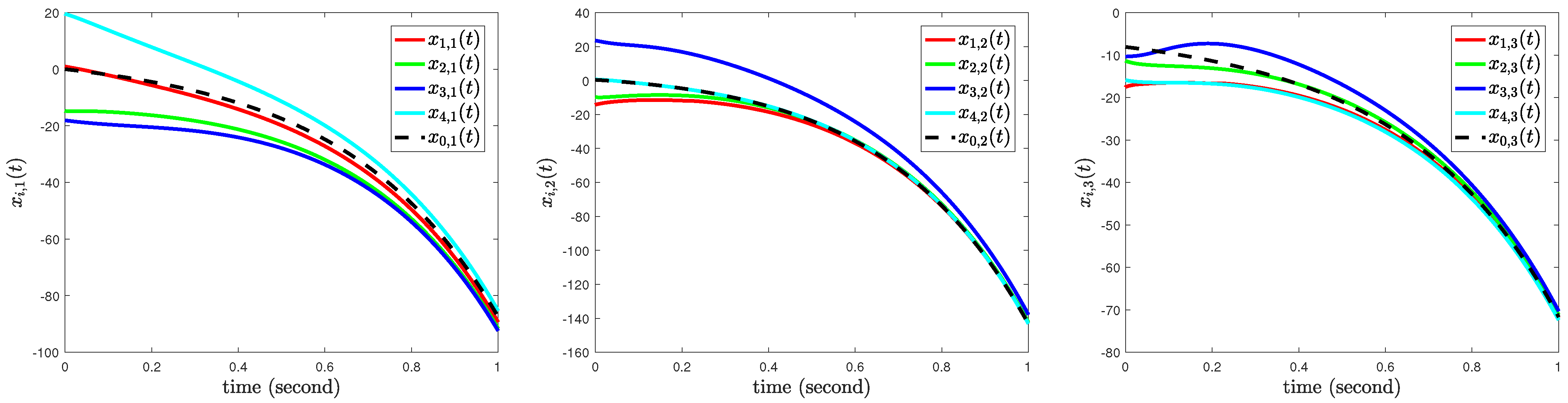
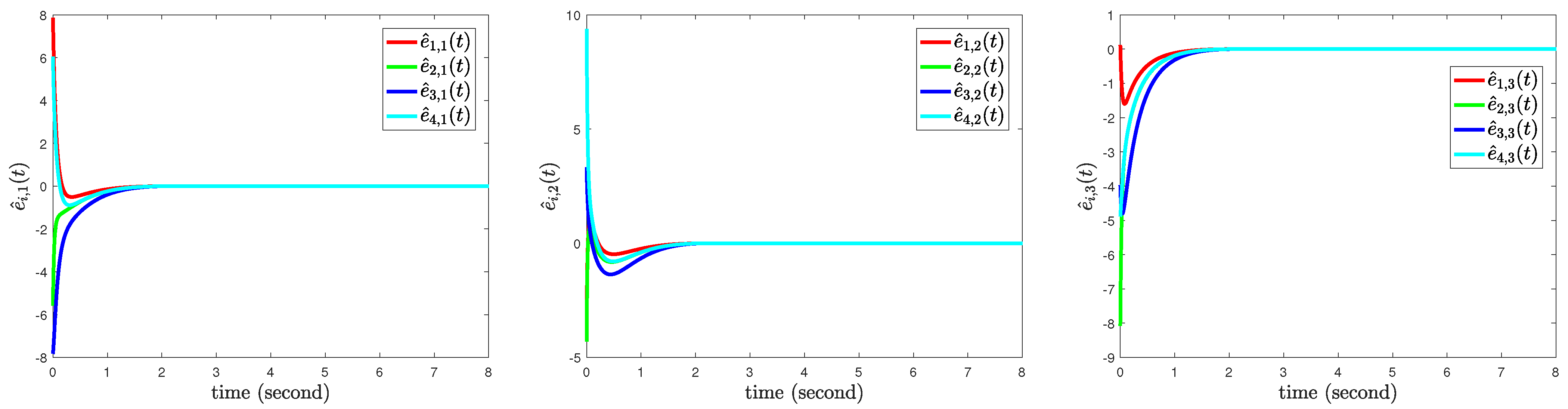
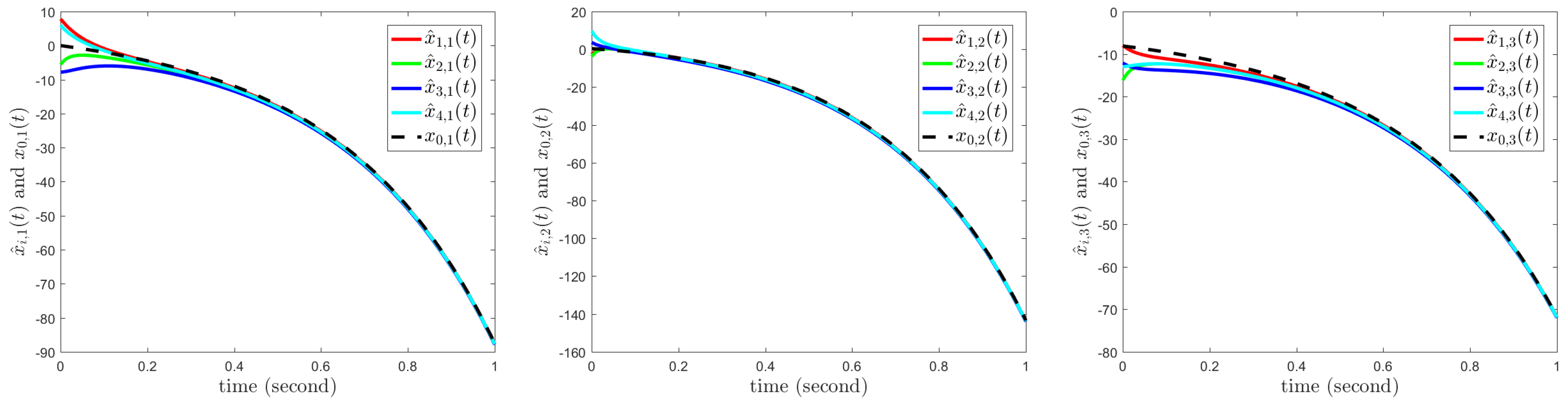
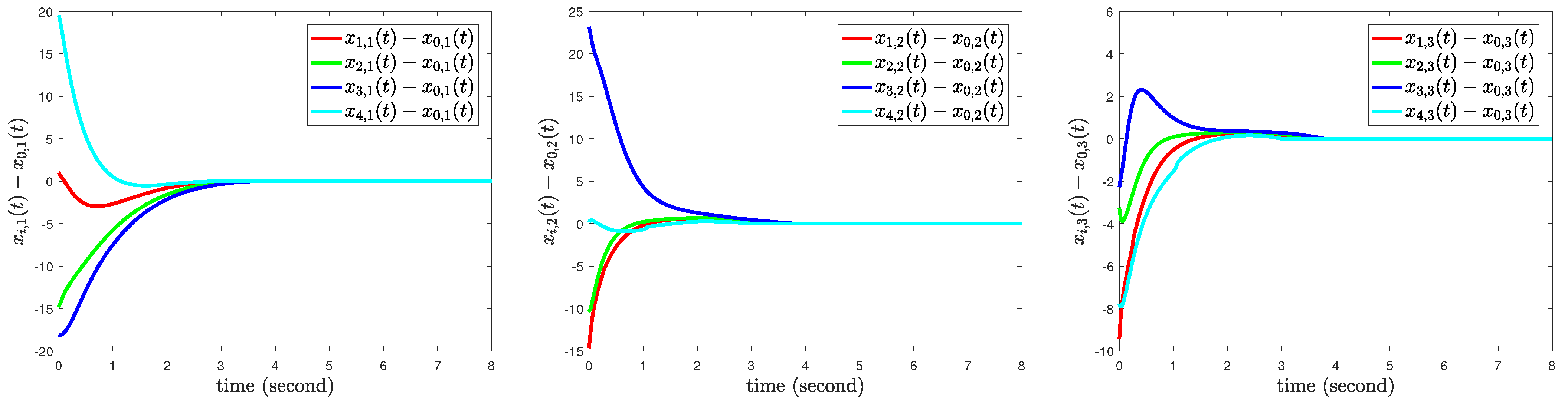
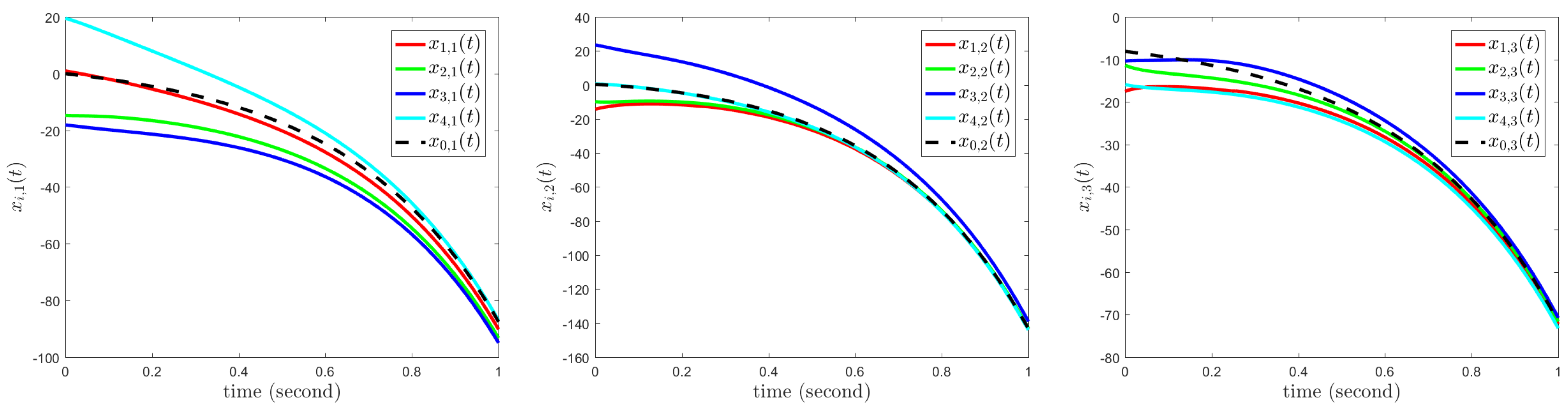
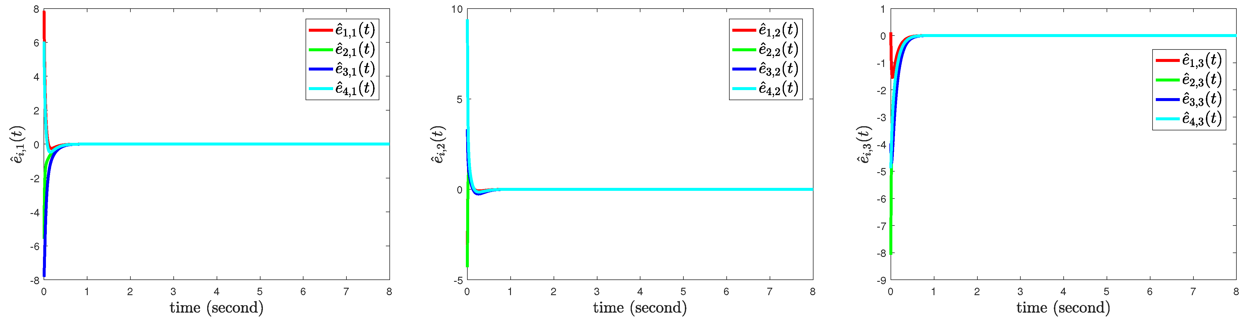
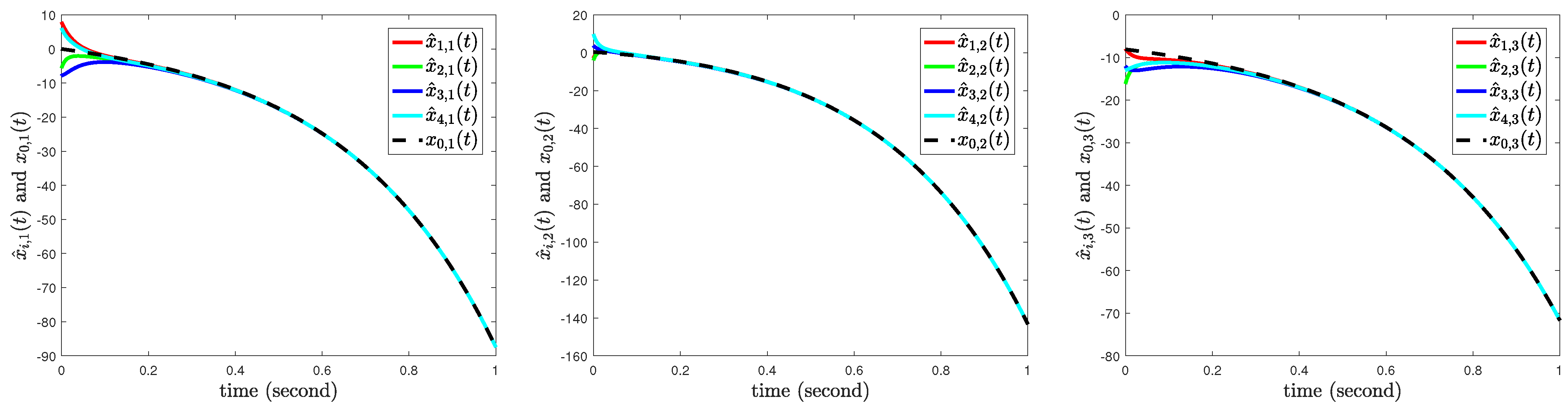
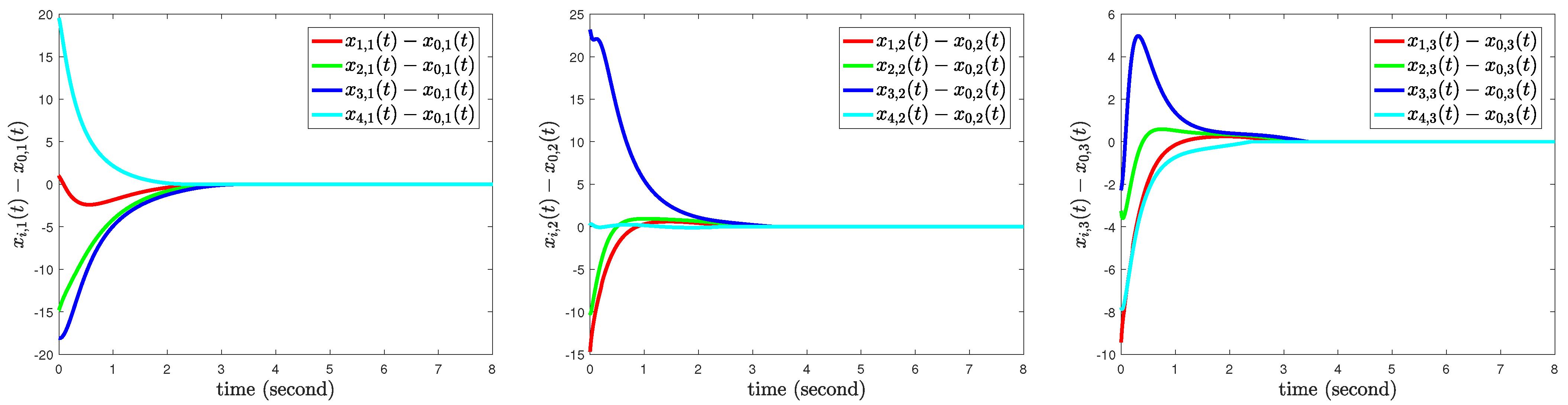
Figure 1 and Figure 2 present the observer’s leader-tracking results: Figure 1 plots the observer–leader state errors over time, and Figure 2 shows their state trajectories. Figure 3 and Figure 4 depict followers’ leader-tracking performance: Figure 3 illustrates follower–leader state errors versus time, and Figure 4 displays all state trajectories of followers and the leader. As can be observed from the results in Figure 1, Figure 2, Figure 3 and Figure 4 (${\varkappa }_i(t)={[{\varkappa }_{i,1}(t),{\varkappa }_{i,2}(t),{\varkappa }_{i,3}(t)]}^T$ for $\varkappa =x,\widehat{x},\widehat{e}$ and $i=0,1,2,3,4$), MASs (1) can achieve fixed-time quasi-consensus with observer (4) and controller (33).

6.1.2. Under DoS Attacks

Consider MASs (1) under DoS attacks as follows:

$$\begin{array}{c}\hfill T_{\mathrm{without}}={\displaystyle \bigcup _{r=0}^{\infty }}[rT,(r+\rho )T),T_{\mathrm{under}}={\displaystyle \bigcup _{r=0}^{\infty }}[(r+\rho )T,(r+1)T),T=2\mathrm{s},\rho =0.6.\end{array}$$

Based on Proposition 2 and Theorem 1, choose (10) and (33) as the observer and controller, respectively, with the parameters given as follows:

$$\begin{array}{cc}\hfill & {\widehat{\kappa }}_1=1,{\widehat{\kappa }}_2=1,{\widehat{\kappa }}_3=24,\hfill \\ \hfill & {\widehat{r}}_1=r_1=q_1=0.5,{\widehat{r}}_2=r_2=q_2=1.5,\hfill \\ \hfill & {\kappa }_1={\kappa }_2={\eta }_1={\eta }_2=1,{ϵ}_{i,p}=0.0001.\hfill \end{array}$$

Figure 5 plots the observer-leader state errors over time, and Figure 6 shows their state trajectories. Figure 7 illustrates follower–leader state errors versus time, and Figure 8 displays all state trajectories of followers and the leader. As can be observed from the results in Figure 5, Figure 6, Figure 7 and Figure 8 (${\varkappa }_i(t)={[{\varkappa }_{i,1}(t),{\varkappa }_{i,2}(t),{\varkappa }_{i,3}(t)]}^T$ for $\varkappa =x,\widehat{x},\widehat{e}$ and $i=0,1,2,3,4$), MASs (1) can achieve fixed-time quasi-consensus with observer (10) and controller (33).

The differences in observer parameter selection and corresponding tracking performance (Figure 1 vs. Figure 5, Figure 2 vs. Figure 6) are completely consistent with the theoretical conclusions of Propositions 1 and 2. Specifically, the conditions for guaranteeing fixed-time tracking of the leader’s state differ between attack-free and DoS-attacked scenarios. Condition (7) holds for MASs (1) free of DoS attacks, whereas condition (13) is required for MASs (1) under DoS attacks. Comparison of these two conditions indicates that condition (13) requires a larger value of ${\widehat{\kappa }}_3$. Accordingly, ${\widehat{\kappa }}_3=24$ is set for the DoS-attack scenario, which is significantly larger than the value of ${\widehat{\kappa }}_3=11$ adopted for the attack-free scenario, ensuring effective observer tracking under DoS attacks. Furthermore, this study considers non-periodic unknown DoS attacks. Hence, the parameter selection strategy of observer is adopted to guarantee observer validity even under worst-case attack conditions, which introduces inherent conservatism into the parameter design for DoS-attacked cases. Simulation comparisons (Figure 1 vs. Figure 5, Figure 2 vs. Figure 6) clearly verify that observers with such conservative parameters achieve faster convergence of the leader’s state. Reducing the conservatism of the existing parameter selection scheme will be a direction for future research.

6.2. Fixed-Time Quasi-Containment Control

Consider MASs (1) with two leaders and four followers. $H_1$ and $H_2$ are given as follows:

$$H_1=\left[\begin{array}{cccc}2& 0& 0& -1\\ 0& 3& -1& -1\\ 0& -1& 1& 0\\ -1& -1& 0& 2\end{array}\right],H_2=\left[\begin{array}{cc}-1& 0\\ 0& -1\\ 0& 0\\ 0& 0\end{array}\right].$$

6.2.1. Without DoS Attacks

Consider MASs (1) without DoS attacks. Based on Proposition 3 and Theorem 2, choose (19) and (33) as the observer and controller, respectively, with the parameters given as follows:

$$\begin{array}{cc}\hfill & {\widehat{\kappa }}_1=1,{\widehat{\kappa }}_2=1,{\widehat{\kappa }}_3=11,\hfill \\ \hfill & {\widehat{r}}_1=r_1=q_1=0.5,{\widehat{r}}_2=r_2=q_2=1.5,\hfill \\ \hfill & {\kappa }_1={\kappa }_2={\eta }_1={\eta }_2=1,{ϵ}_{i,p}=0.0001.\hfill \end{array}$$

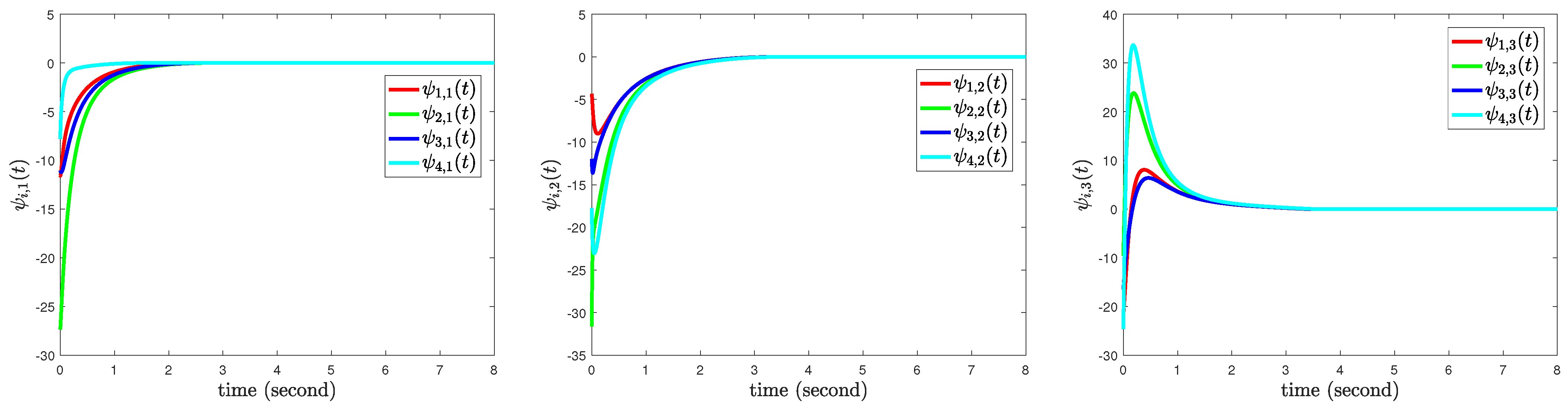
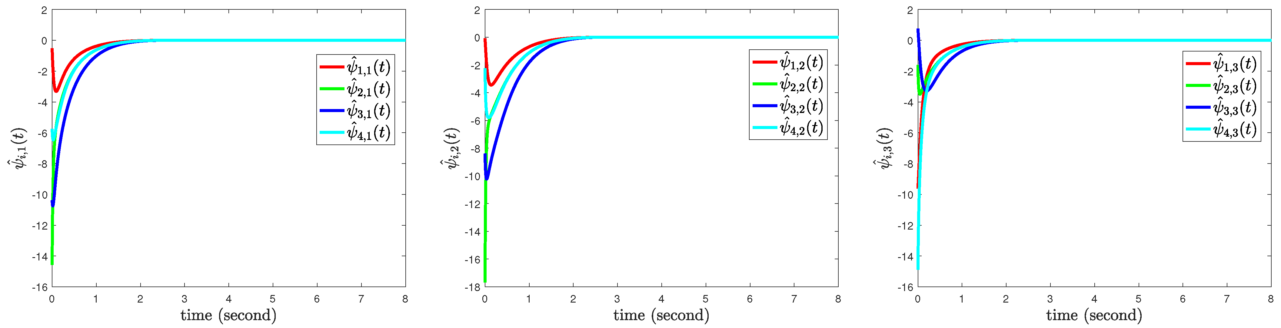
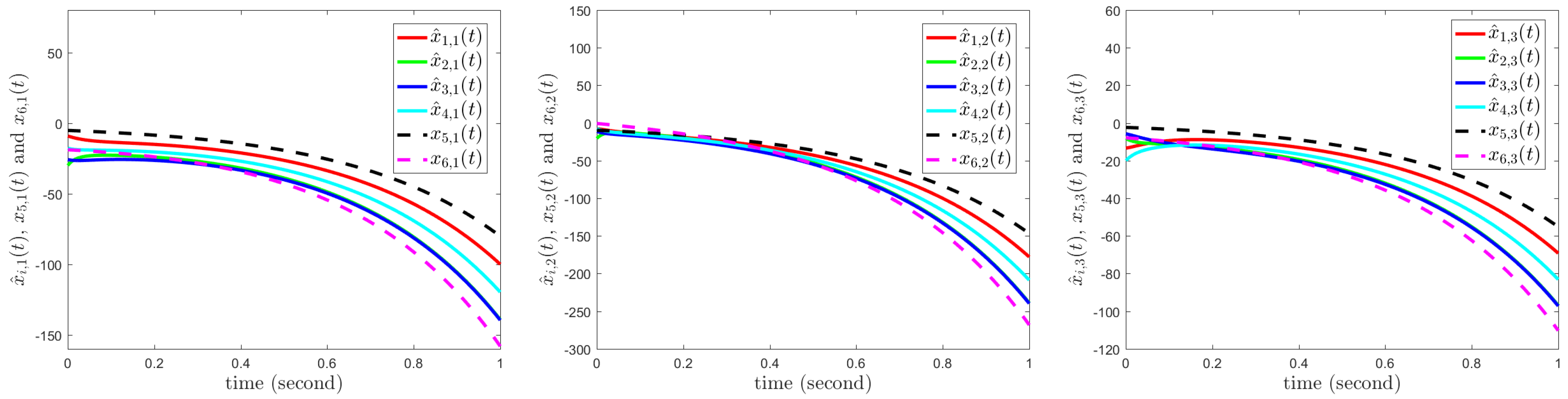
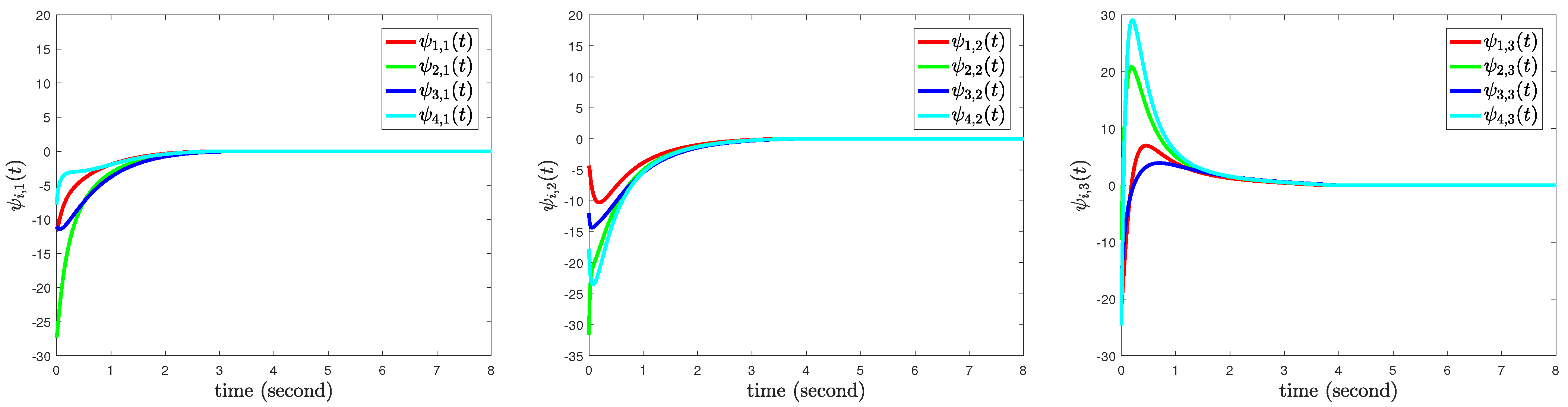
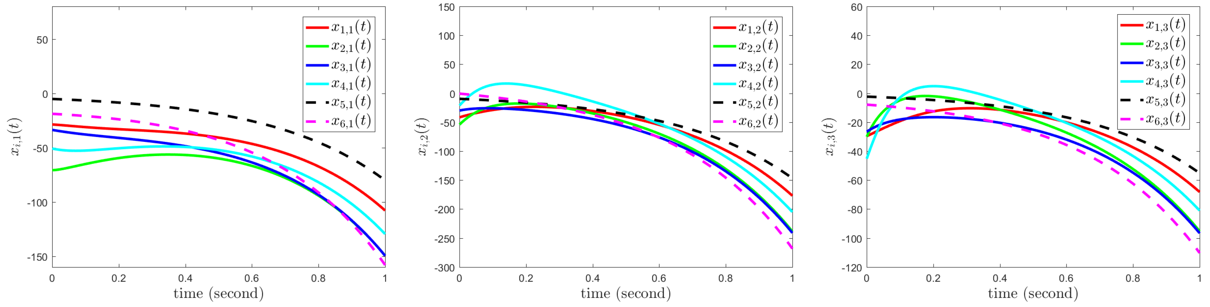
Figure 9 and Figure 10 present the observer’s leader-tracking results. Figure 11 and Figure 12 depict followers’ leader-tracking performance. As can be observed from the results in Figure 9, Figure 10, Figure 11 and Figure 12 (${\varkappa }_i(t)={[{\varkappa }_{i,1}(t),{\varkappa }_{i,2}(t),{\varkappa }_{i,3}(t)]}^T$ for $\varkappa =x,\widehat{x},\psi ,\widehat{\psi }$ and $i=1,2,3,4,5,6$), MASs (1) can achieve fixed-time quasi-containment control with observer (19) and controller (33).

6.2.2. Under DoS Attacks

Consider MASs (1) under DoS attacks as follows:

$$\begin{array}{c}\hfill T_{\mathrm{without}}={\displaystyle \bigcup _{r=0}^{\infty }}[rT,(r+\rho )T),T_{\mathrm{under}}={\displaystyle \bigcup _{r=0}^{\infty }}[(r+\rho )T,(r+1)T),T=2\mathrm{s},\rho =0.6.\end{array}$$

Based on Proposition 4 and Theorem 2, choose (25) and (33) as the observer and controller, respectively, with the parameters given as follows:

$$\begin{array}{cc}\hfill & {\widehat{\kappa }}_1=1,{\widehat{\kappa }}_2=1,{\widehat{\kappa }}_3=24,\hfill \\ \hfill & {\widehat{r}}_1=r_1=q_1=0.5,{\widehat{r}}_2=r_2=q_2=1.5,\hfill \\ \hfill & {\kappa }_1={\kappa }_2={\eta }_1={\eta }_2=1,{ϵ}_{i,p}=0.0001.\hfill \end{array}$$

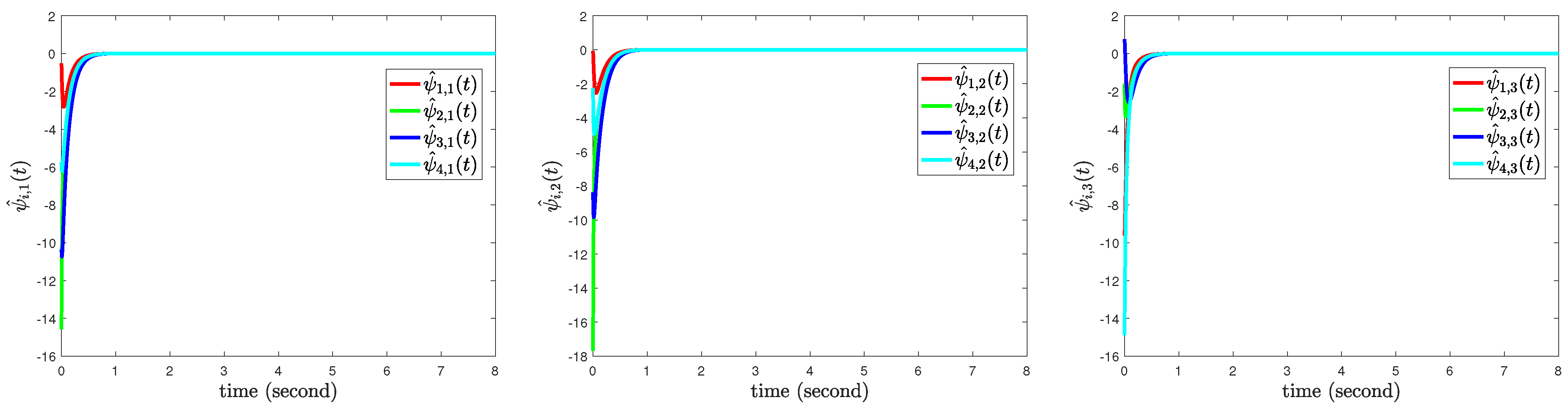
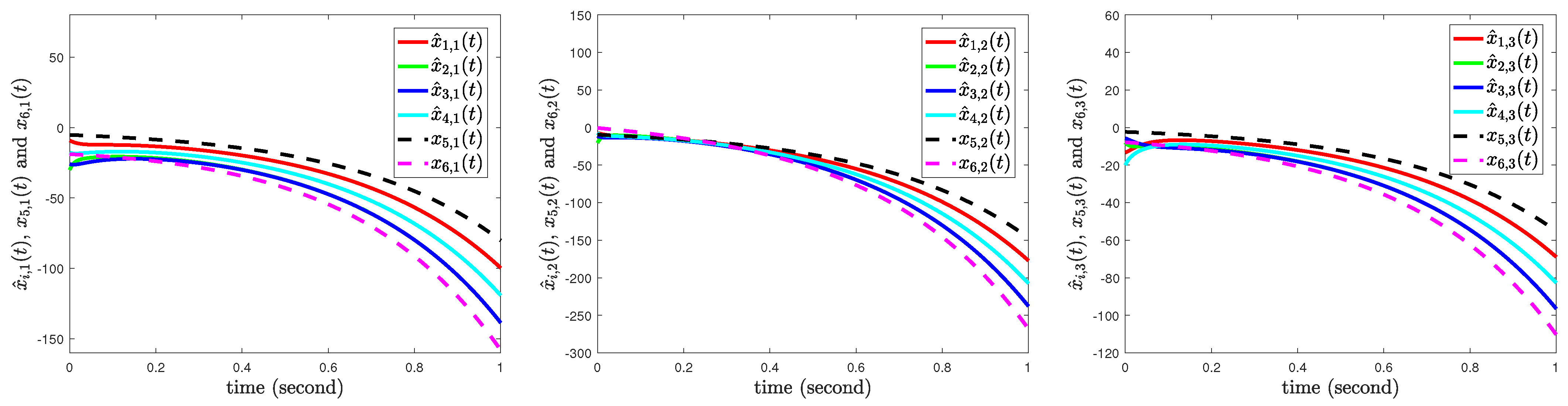
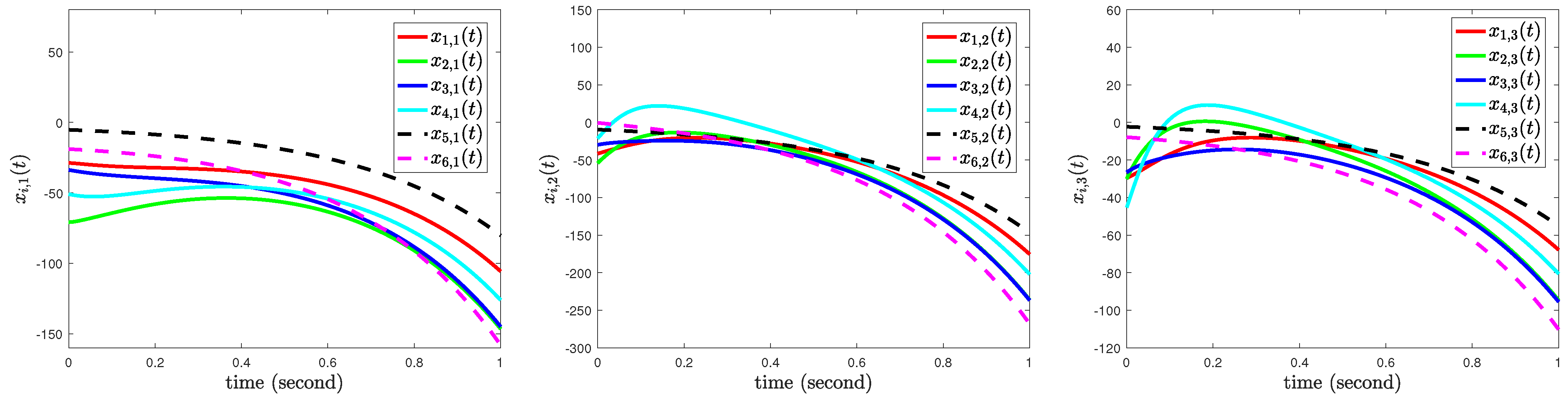
Figure 13 and Figure 14 present the observer’s leader-tracking results. Figure 15 and Figure 16 depict followers’ leader-tracking performance. As can be observed from the results in Figure 13, Figure 14, Figure 15 and Figure 16 (${\varkappa }_i(t)={[{\varkappa }_{i,1}(t),{\varkappa }_{i,2}(t),{\varkappa }_{i,3}(t)]}^T$ for $\varkappa =x,\widehat{x},\psi ,\widehat{\psi }$ and $i=1,2,3,4,5,6$), MASs (1) can achieve fixed-time quasi-containment control with observer (25) and controller (33).

Remark 8.

In this study, all simulation parameters are strictly selected according to the established theoretical assumptions, propositions, and theorems. Specifically, the system A and input B matrices are chosen to satisfy Assumption 3, which guarantees the feasibility and effectiveness of the designed controller as required by Theorems 1 and 2; the topology matrices $H_1$ and $H_2$ are constructed following Assumption 1 to ensure the connectivity of the communication network in the attack-free case; the DoS attack parameters $T=2\mathit{seconds}$ and $\rho =0.6$ (corresponding to $\tau =0.6$) are configured to strictly satisfy the constraint conditions in Assumption 2; setting ${ϵ}_{i,p}=0.0001$ ensures a sufficiently small error; and all observer and controller gains are obtained from the feasible conditions derived from Propositions 1–4 and Theorems 1 and 2.

7. Conclusions

In this study, the problems of fixed-time quasi-consensus and quasi-containment control for MASs are studied. First, considering both scenarios where the MASs (1) are subject to and free of DoS attacks, the corresponding observers are designed to enable accurate tracking of leader information within a fixed time. Second, the controller is designed via the linear transformation of state space and the construction of sliding surfaces. Even when the input matrix is not an invertible square matrix, the MASs can still realize fixed-time quasi-consensus and quasi-containment control. Finally, the numerical examples are provided to verify the obtained results. Compared with the existing literature, the proposed method possesses unique applicability advantages in handling coupled harsh constraints. Most existing fixed-time cooperative control schemes can only cope with ideal input matrices or attack-free environments and cannot simultaneously address unknown non-periodic DoS attacks and non-invertible non-square input matrices. Against this background, this study provides two main contributions. First, a fixed-time observer is designed to track leader state information under unknown non-periodic DoS attacks. Second, a novel controller is developed to realize fixed-time quasi-consensus and quasi-containment control for MASs with non-invertible, non-square input matrices under mild conditions. Nevertheless, this method also has evident limitations: the strict accurate fixed-time consensus and containment control cannot be realized, and the adopted continuous control strategy brings heavy communication burden. Future work will focus on control schemes for switched stochastic MASs based on event-triggered communication.

References

1. Olfati-Saber, R.; Murray, R.M. Distibuted cooperative control of multiple vehicle formations using structural potential functions. In Proceedings of the 15th IFAC World Congress, Barcelona, Spain, 21–26 July 2002. [Google Scholar]
2. Vidal, R.; Shakernia, O.; Sastry, S. Formation control of nonholonomic mobile robots omnidirectional visual servoing and motion segmentation. IEEE Int. Conf. Robot. Autom. 2003, 1, 584–589. [Google Scholar] [CrossRef] [Scilit]
3. Lawton, J.R.; Bread, R.W. Synchronized multiple spacecraft rotations. Automatica 2002, 38, 1359–1364. [Google Scholar] [CrossRef] [Scilit]
4. Olfati-Saber, R.; Murray, R.M. Consensus problems in networks of agents with switching topology and time-delays. IEEE Trans. Autom. Control 2004, 49, 1520–1533. [Google Scholar] [CrossRef] [Scilit]
5. Yang, H.; Zhang, Z.; Zhang, S. Consensus of second-order multi-agent systems with exogenous disturbances. Int. J. Robust Nonlinear Control 2011, 21, 945–956. [Google Scholar] [CrossRef] [Scilit]
6. Li, Z.; Duan, Z.; Ren, W.; Feng, G. Containment control of linear multi-agent systems with multiple leaders of bounded inputs using distributed continuous controllers. Int. J. Robust Nonlinear Control 2015, 25, 2101–2121. [Google Scholar] [CrossRef] [Scilit]
7. Zhang, H.; Han, J.; Wang, Y.; Jiang, H. H consensus for linear heterogeneous discrete-time multiagent systems with output feedback control. IEEE Trans. Cybern. 2019, 49, 3713–3721. [Google Scholar] [CrossRef] [Scilit] [PubMed]
8. Yaghmaie, F.A.; Lewis, F.L.; Su, R. Output regulation of linear heterogeneous multi-agent systems via output and state feedback. Automatica 2016, 67, 157–164. [Google Scholar] [CrossRef] [Scilit]
9. Wang, Z.; He, H. Asynchronous quasi-consensus of heterogeneous multiagent systems with nonuniform input delays. IEEE Trans. Syst. Man Cybern. Syst. 2020, 50, 2815–2827. [Google Scholar]
10. Guo, G.; Tan, H.; Feng, Y.; Wang, Y. Event-triggered super-twisting fixed-time consensus control for networked nonlinear multi-agent systems with disturbance. IEEE Trans. Autom. Sci. Eng. 2025, 22, 11920–11932. [Google Scholar] [CrossRef] [Scilit]
11. Liu, L.; Sun, H.; Ma, L.; Zhang, J.; Bo, Y. Quasi-consensus control for a class of time-varying stochastic nonlinear time-delay multiagent systems subject to deception attacks. IEEE Trans. Syst. Man Cybern. Syst. 2021, 51, 6863–6873. [Google Scholar] [CrossRef] [Scilit]
12. Xu, Y.; Fang, M.; Shi, P.; Wu, Z. Event-based secure consensus of mutiagent systems against DoS attacks. IEEE Trans. Cybern. 2020, 50, 3468–3476. [Google Scholar] [CrossRef] [Scilit] [PubMed]
13. Yang, Y.; Li, Y.; Yue, D.; Tian, Y.C.; Ding, X. Distributed secure consensus control with event-triggering for multiagent systems under DoS attacks. IEEE Trans. Cybern. 2021, 51, 2916–2928. [Google Scholar] [CrossRef] [Scilit] [PubMed]
14. Zhu, G.; Tian, B.; Zhang, X.; Su, C.Y. Dynamic event-triggered performance control for heterogeneous multi-agent systems under DoS attacks and its application. Inf. Sci. 2026, 754, 123740. [Google Scholar] [CrossRef] [Scilit]
15. Zhang, T.Y.; Ye, D. Distributed event-triggered control for multi-agent systems under intermittently random denial-of-service attacks. Inf. Sci. 2021, 542, 380–390. [Google Scholar] [CrossRef] [Scilit]
16. Shang, Y.; Liu, C.L.; Cao, K.C. Event-triggered consensus control of second-order nonlinear multi-agent systems under denial-of-service attacks. Trans. Inst. Meas. Control 2021, 43, 2272–2281. [Google Scholar] [CrossRef] [Scilit]
17. Lu, D.; Zhang, H.; Zhang, Q.; Bo, C. Observer-based event-triggered secure control for networked nonlinear systems under denial-of-service attacks. Actuators 2026, 15, 369. [Google Scholar] [CrossRef] [Scilit]
18. Liu, L.; Yan, B.; Ni, J.; Shi, P. Neural-network-based event-triggered consensus tracking for nonlinear heterogeneous multi-agent systems against denial-of-service attacks. Int. J. Robust Nonlinear Control 2026, in press. [Google Scholar] [CrossRef] [Scilit]
19. Zhang, Y.; Wu, Z.; Shi, P.; Huang, T.; Chakrabarti, P. Quantization-based event-triggered consensus of multiagent systems against aperiodic DoS attacks. IEEE Trans. Syst. Man Cybern. Syst. 2023, 53, 3774–3783. [Google Scholar] [CrossRef] [Scilit]
20. Deng, C.; Wen, C. MAS-based distributed resilient control for a class of cyber-physical systems with communication delays under DoS attacks. IEEE Trans. Cybern. 2021, 51, 2347–2358. [Google Scholar] [CrossRef] [Scilit] [PubMed]
21. Guadarrama-Estrada, A.R.; Osorio-Gordillo, G.L.; Sename, O.; Vargas-Méndez, R.A.; Astorga-Zaragoza, C.M.; Reyes-Reyes, J.; Serrano-Cruz, D.A.; Pineda-Uribe, A. Resilient state and attack estimation in discrete Markovian cyber-physical systems via generalized dynamic observers. Electronics 2026, 15, 2824. [Google Scholar] [CrossRef] [Scilit]
22. Sakthivel, R.; Sakthivel, R.; Kaviarasan, B.; Lee, H.; Lim, Y. Finite-time leaderless consensus of uncertain multi-agent systems against time-varying actuator faults. Neurocomputing 2019, 325, 159–171. [Google Scholar] [CrossRef] [Scilit]
23. Li, Y.; Li, Y.X.; Tong, S. Event-based finite-time control for nonlinear multiagent systems with asymptotic tracking. IEEE Trans. Autom. Control 2023, 68, 3790–3797. [Google Scholar] [CrossRef] [Scilit]
24. Han, J.; Jiang, H.; Zhao, Y. Fixed-time consensus problem for uncertain multi-agent systems with continuous and intermittent control. J. Frankl. Inst. 2024, 361, 107179. [Google Scholar] [CrossRef] [Scilit]
25. Baradarannia, M.; Hashemzadeh, F.; Kumbasar, T. Fixed-time surrounding control of multi-agent systems under denial-of-service attacks. J. Frankl. Inst. 2025, 362, 108095. [Google Scholar] [CrossRef] [Scilit]
26. Xu, L.; Xi, H.; Zhao, J. Practically fixed-time H deployment of large-scale heterogeneous multi-agent systems with multiple dimensions via a PDE-based approach. Expert Syst. Appl. 2026, 317, 131760. [Google Scholar] [CrossRef] [Scilit]
27. Liu, M.; Guo, Y.; Ran, G.; Park, J.H. Fixed-time consensus tracking control for nonlinear multi-agent systems: A dynamic edge/self-triggered approach. IEEE Trans. Circuits Syst. II Express Briefs 2026, 73, 73–77. [Google Scholar] [CrossRef] [Scilit]
28. Wang, L.; Yan, H.; Hu, X.; Li, Z.; Wang, M. Fixed-time bipartite containment control for heterogeneous multiagent systems under DoS attacks: An event-triggered mechanism. IEEE Trans. Syst. Man Cybern. Syst. 2025, 55, 2782–2794. [Google Scholar] [CrossRef] [Scilit]
29. Cai, Y.; Zhang, H.; Wang, Y.; Zhang, J.; He, Q. Fixed-time time-varying formation tracking for nonlinear multiagent systems under event-triggered mechanism. Inf. Sci. 2021, 564, 45–70. [Google Scholar] [CrossRef] [Scilit]
30. Zhou, S.; Deng, C.; Fan, S.; Wang, B. Fixed-time resilient distributed NE seeking control for nonlinear MASs against DoS attacks. IEEE Trans. Cybern. 2025, 55, 3368–3378. [Google Scholar] [CrossRef] [Scilit] [PubMed]
31. Zhao, L.; Lu, J.; Ruan, Q.; Huang, T. Energy metrics and tradeoff of nonlinear multi-agent consensus subject to DoS attacks. Inf. Sci. 2025, 718, 122362. [Google Scholar] [CrossRef] [Scilit]
32. Han, J.; Jiang, H.; Zhao, Y.; Shi, J. Fixed-time event-triggered and periodic event-triggered containment control for heterogeneous multi-agent systems under DoS attacks. Syst. Control Lett. 2025, 204, 106208. [Google Scholar] [CrossRef] [Scilit]
33. Veisi, A.; Delavari, H. Deep reinforcement learning-based robust nonlinear controller for photovoltaic systems. Neural Comput. Appl. 2024, 36, 19989–20009. [Google Scholar] [CrossRef] [Scilit]
34. Veisi, A.; Delavari, H. Intelligent model-free data-driven robust control based on fractional reinforcement learning. Int. J. Robust Nonlinear Control 2026, 36, 1982–2000. [Google Scholar] [CrossRef] [Scilit]
35. Xing, M.; Lu, J.; Liu, Y.; Chen, X. Event-based bipartite consensus of multi-agent systems subject to DoS attacks. IEEE Trans. Netw. Sci. Eng. 2023, 10, 68–80. [Google Scholar] [CrossRef] [Scilit]
36. Hui, M.; Liu, X.; Cao, J. Improved fixed-time event-triggered average consensus of multi-agent systems under DoS attacks. IEEE Trans. Circuits Syst. II Express Briefs 2024, 71, 3815–3819. [Google Scholar] [CrossRef] [Scilit]
37. Hou, L.; Lan, X.; Ren, Y.; Zhang, P. Fixed-time consensus protocols of multiagent systems based speed coordinated control for multiple permanent magnet synchronous motors under vector control system. IEEE Trans. Power Electron. 2025, 40, 17844–17857. [Google Scholar] [CrossRef] [Scilit]
38. Liu, Y.; Zhang, H.; Sun, J.; Wang, Y. Event-triggered adaptive finite-time containment control for fractional-order nonlinear multiagent systems. IEEE Trans. Cybern. 2024, 54, 1250–1260. [Google Scholar] [CrossRef] [Scilit] [PubMed]
39. Ning, B.; Jin, J.; Zheng, J.; Man, Z. Finite-time and fixed-time leader-following consensus for multi-agent systems with discontinuous inherent dynamics. Int. J. Control 2017, 91, 1259–1270. [Google Scholar] [CrossRef] [Scilit]
40. Wonham, W.M.; Morse, A.S. Decoupling and pole assignment in linear multivariable systems: A geometric approach. SIAM J. Control 1970, 8, 1–18. [Google Scholar] [CrossRef] [Scilit]
41. Qin, J.; Ma, Q.; Yu, X.; Kang, Y. Output containment control for heterogeneous linear multiagent systems with fixed and switching topologies. IEEE Trans. Cybern. 2019, 49, 4117–4128. [Google Scholar] [CrossRef] [Scilit] [PubMed]
42. Cao, Y.; Ren, W.; Egerstedt, M. Distributed containment control with multiple stationary or dynamic leaders in fixed and switching directed networks. Automatica 2012, 48, 1586–1597. [Google Scholar] [CrossRef] [Scilit]
43. Yang, Y.; Wang, Z.; Jin, W. Security containment control for nonlinear MASs under DOS attacks: An improved adaptive method. Neurocomputing 2024, 610, 128601. [Google Scholar] [CrossRef] [Scilit]
44. Gambuzza, L.V.; Buscarino, A.; Fortuna, L.; Frasca, M. Memristor-based adaptive coupling for consensus and synchronization. IEEE Trans. Circuits-Syst.-I Regul. Pap. 2015, 62, 1175–1184. [Google Scholar] [CrossRef] [Scilit]
Figure 1. The trajectory of e ^ i ( t ) with observer (4) and controller (33).
Mathematics 14 02989 g001
Figure 2. The trajectories of x ^ i ( t ) and x 0 ( t ) with observer (4) and controller (33).
Mathematics 14 02989 g002
Figure 3. The trajectory of x i ( t ) x 0 ( t ) with observer (4) and controller (33).
Mathematics 14 02989 g003
Figure 4. The trajectories of x i ( t ) and x 0 ( t ) with observer (4) and controller (33).
Mathematics 14 02989 g004
Figure 5. The trajectory of e ^ i ( t ) with observer (10) and controller (33).
Mathematics 14 02989 g005
Figure 6. The trajectories of x ^ i ( t ) and x 0 ( t ) with observer (10) and controller (33).
Mathematics 14 02989 g006
Figure 7. The trajectory of x i ( t ) x 0 ( t ) with observer (10) and controller (33).
Mathematics 14 02989 g007
Figure 8. The trajectories of x i ( t ) and x 0 ( t ) with observer (10) and controller (33).
Mathematics 14 02989 g008
Figure 9. The trajectory of ψ ^ i ( t ) with observer (19) and controller (33).
Mathematics 14 02989 g009
Figure 10. The trajectories of x ^ i ( t ) , x 5 ( t ) and x 6 ( t ) with observer (19) and controller (33).
Mathematics 14 02989 g010
Figure 11. The trajectory of ψ ( t ) with observer (19) and controller (33).
Mathematics 14 02989 g011
Figure 12. The trajectory of x i ( t ) with observer (19) and controller (33).
Mathematics 14 02989 g012
Figure 13. The trajectory of ψ ^ i ( t ) with observer (25) and controller (33).
Mathematics 14 02989 g013
Figure 14. The trajectories of x ^ i ( t ) , x 5 ( t ) and x 6 ( t ) with observer (25) and controller (33).
Mathematics 14 02989 g014
Figure 15. The trajectory of ψ ( t ) with observer (25) and controller (33).
Mathematics 14 02989 g015
Figure 16. The trajectory of x i ( t ) with observer (25) and controller (33).
Mathematics 14 02989 g016
Disclaimer/Publisher’s Note: The statements, opinions and data contained in all publications are solely those of the individual author(s) and contributor(s) and not of MDPI and/or the editor(s). MDPI and/or the editor(s) disclaim responsibility for any injury to people or property resulting from any ideas, methods, instructions or products referred to in the content.