ILP Formulation and Exact Solution of Multicast Routing with Fairness

Abstract

Fairness is critical in delay-sensitive group applications—multiplayer online games, live collaborative editing, and distributed interactive simulations—where every participant should receive each message within a bounded delay and with minimal timing differences between recipients. We study fairness-aware multicast routing under two parameters: the maximum end-to-end delay ($\Delta$) and the inter-destination delay variation ($\delta$). Although several heuristics address this NP-hard problem and exact integer linear programs (ILPs) exist for the minimum-cost multi-constrained case, exact methods that directly optimize inter-destination delay variation under bounded delay remain underexplored. We present flow-based ILP formulations that treat $\Delta$ and $\delta$ as either objectives or constraints. Their feasible solutions are partial spanning hierarchies, a class that contains partial spanning trees as a special case; consequently a hierarchy optimum is, by construction, at least as good as the best tree-constrained solution. On proven-optimal instances, hierarchy optima reduce inter-destination delay variation considerably relative to the best tree-constrained solution. A sensitivity analysis, a real-topology study on the Abilene backbone, and an exact-ILP scalability study quantify and corroborate these gains.

1. Introduction

In many modern applications, such as multiplayer online games, live collaborative editing sessions, and distributed interactive simulations, maintaining fairness in message delivery is crucial for user experience. When some participants receive messages later than others, the perceived unfairness can undermine the effectiveness of the application. This paper addresses the challenge of route selection that controls delay dispersion among recipients while ensuring that an absolute delay ceiling is not exceeded. Formal definitions of the two delay-related fairness metrics—maximum end-to-end delay ($\Delta$) and inter-destination delay variation ($\delta$)—are given in Section 2.1.

The same two-parameter requirement, a bounded worst-case delay $\Delta$ and a bounded inter-recipient skew $\delta$, appears in many contexts beyond these examples. This broad applicability highlights the value of an exact approach. In synchronous distributed and federated machine learning, an aggregation round closes only after the slowest worker finishes reporting. Therefore, bounding the spread of per-worker update-arrival times under a round deadline directly addresses delay variation; mitigating such stragglers is a central concern in large-scale synchronous stochastic gradient descent [1,2]. In financial market data dissemination, exchanges must deliver price feeds to competing participants with nearly equal latency to prevent any recipient from gaining an information advantage.

Recent cloud-exchange designs explicitly address this as fair multicast with bounded inter-receiver latency variance [3,4]. In multi-agent robotics, a control command that reaches swarm agents with large skew degrades formation stability, so a bounded $\Delta$ with small $\delta$ becomes a safety requirement [5]. Related fairness-of-arrival concerns arise in blockchain block propagation, where low-variation dissemination limits the advantage of topologically well-positioned nodes [6], and in synchronized live-event delivery, where earlier receipt confers an unfair edge. In each case, the routing structure that serves the group fixes the achievable $(\Delta ,\delta )$ trade-off, and a certified optimum—rather than a heuristic—carries direct operational stakes. Route selection is an effective mechanism for achieving fairness within a user group. Multicast routing has been proposed for this type of communication (cf. [7]). The combination of cost minimization and fairness criteria results in a multi-constrained Steiner problem. From a computational perspective, this corresponds to a class of NP-hard combinatorial optimization problems, closely related to constrained Steiner trees and network design formulations. Several useful heuristics have been proposed, and exact integer linear programs have been developed for the minimum-cost multi-constrained version of the problem [8,9]. However, the optimization of inter-destination delay variation has not been thoroughly analyzed. Routing is not the only mechanism for handling fairness; scheduling and rate control are complementary approaches. This paper focuses on the route-selection dimension.

Exact formulations are valuable because they provide theoretical insights into problem complexity and benchmarks for evaluating heuristic or metaheuristic methods. Additionally, they enable systematic exploration of trade-offs among cost, delay, and inter-destination delay variation. This paper addresses this gap by presenting exact formulations of fairness-aware multicast routing using integer linear programming. These formulations minimize both end-to-end delay and inter-destination delay variation while satisfying cost and feasibility constraints.

To address fairness in group communication, a summary of optimal route computations based on integer linear programming (ILP) is provided. Some of these formulations correspond to multi-objective optimization, while others are multi-constrained. Consistent with established results for minimum-cost multi-constrained multicast [8,9], optimal routes are often sub-networks known as partial spanning hierarchies rather than multicast trees. The key innovation here is that applying this relaxation to the delay-variation objective broadens the feasible region and produces solutions with provably lower variation (cf. Section 3). A concise case study demonstrates these hierarchies as effective multicast routing structures.

The remainder of the paper is organized as follows. Section 2 introduces the basic problem, provides formal definitions, and reviews relevant related work. Section 3 highlights the benefits of general sub-network-based solutions compared to classical multicast trees. Section 4 presents several fairness-aware routing formulations using linear programming techniques. Section 5 presents the experimental evaluation on minimizing inter-destination delay variation under various delay bounds. Finally, Section 6 concludes the paper and outlines possible directions for future research.

This work positions the delay bound $\Delta$ and the variation bound $\delta$ as operational fairness constraints grounded in the equitable-optimization literature: $\Delta$ corresponds to the lexicographic maximin (Rawlsian) criterion [10,11] and $\delta$ to the bounded-inequality/no-envy-within-threshold principle [12,13] (see the axiomatic foundations in Section 2). Against that backdrop, the main contributions are the following.

• Structural characterization of the feasible region (Proposition 1). The feasible region of partial spanning hierarchies contains that of partial spanning trees under any fairness bounds $(\Delta ,\delta )$, so the induced inequality ${\delta }_H^{*}\le {\delta }_T^{*}$ holds by construction. Part (ii) exhibits a bottleneck-instance family on which the containment is strict, and part (iii)—together with the accompanying Remark 1—states a sufficient condition under which the gap is quantifiable.
• Exact ILP formulations. A family of flow-based integer linear programming models, applicable to multi-objective and multi-constrained settings, yields provably optimal fairness-aware multicast routes. A single constraint skeleton hosts all four objectives (cost, per-destination delay, maximum delay, and maximum pairwise variation) and toggles between the hierarchy and tree feasible regions through one single-predecessor constraint, so that tree-versus-hierarchy comparisons are controlled experiments within one model rather than comparisons across unrelated formulations. Unlike previous work, these formulations serve as ground-truth benchmarks rather than heuristic approximations.
• Computational study. A cross-topology comparison (Section 5.1), a six-parameter sensitivity analysis (Section 5.2), a 120-instance distribution of the exact tree–hierarchy gap (Section 5.3), a real-topology evaluation on the Abilene backbone (Section 5.4), and an exact-ILP scalability sweep to $n=20$ (Section 5.5) together quantify the gain the enlargement of the feasible region delivers empirically.
• Heuristic benchmarking. A comparative case study on synthetic network instances benchmarks the ILP optima against CHAINS (a k-shortest-path assembly heuristic [14]), the strongest heuristic in the delay and delay-variation bounded multicast tree (DVBMT) lineage. The ILP-optimal hierarchies match or improve on CHAINS at every tested bound, and the hierarchy advantage over the best tree solution grows as $\Delta$ is relaxed.

2. Problem Formulation and Related Work

This study addresses a specific class of routing problems: fairness-aware multicast routing among users. The scenario involves a designated server distributing messages to multiple users through a multicast route. Fairness is assessed using two primary performance metrics: the end-to-end delay from the server to each user and the variation in these delays across the user set. These metrics are formally defined in Definition 2.

2.1. Notation and Definitions

The analysis is based on a graph model. The network topology is represented as a directed graph. The routing structure for group communication may differ from a classical multicast tree. In particular, optimal routes for fairness are not always trees but may take the form of more general sub-networks, referred to as hierarchies. These hierarchies enable different walks to share common prefixes and reuse arcs, providing greater flexibility in meeting fairness constraints on delay and delay variation. To facilitate the definition of possible exact solutions, the concept of graph hierarchy [15] is introduced. The following presents the directed version of the definition.

Definition 1

(Directed hierarchy). Let $G=(V,A)$ be an arbitrary digraph and $T=(P,F)$ a directed tree. Let $h:P\to V$ be a homomorphic function, which associates a node $v\in V$ to each node $p\in P$. The application $(T,h,G)$ defines a hierarchy in G.

Recall that the homomorphism preserves node adjacency. The result is a structure that behaves like a tree over the graph G but may include shared arcs or repeated nodes. This more general tree structure, called a “non-elementary tree”, enables solutions that standard multicast trees cannot provide. It will be shown that the exact solution to the fair multicast routing problem corresponds to a hierarchy.

Table 1. Summary of Notation.

$G=(V,A)$	Directed graph representing the network topology
$s\in V$	Source node initiating the communication
$M\subset V\setminus \left\{s\right\}$	Set of multicast destination nodes
$T=(V_T,A_T)$	Directed tree
$H=(T,h,G)$	Directed hierarchy (a generalization of a tree using a homomorphism h, cf. Definition 1)
$(u,v)\in A$	Arc from node u to node v
$source\left(a\right)$	Source node of arc a
$target\left(a\right)$	Target node of arc a
$C\left(a\right)$	Cost associated with arc a
$D\left(a\right)$	Transmission delay associated with arc a
$P_{(u,v)}$	Path from node u to node v
$Out\left(u\right)$	Set of arcs outgoing from node u
$In\left(u\right)$	Set of arcs incoming to node u
$\Delta$	Maximum tolerated end-to-end delay
$\delta$	Maximum tolerated inter-destination delay variation
ILP decision variables
$F(m,a)$	Binary—equals 1 if the flow to destination $m\in M$ uses arc $a\in A$ on its path from the source, and 0 otherwise
$x\left(a\right)$	Continuous in $[0, 1]$—equals ${max}_{m\in M}F(m,a)$; pinned by Equations (22) and (23); integrality never required
$\sigma (m,n,a)$	Continuous in $[0, 1]$—equals 1 iff flows to m and n use arc a along a common shared prefix; equals the product $F(m,a)·F(n,a)$ at source arcs (Equation (24)) and is pinned elsewhere by Equations (25)–(27); integrality never required
$d_m$	Continuous—end-to-end delay to destination m

summarizes the main notation used throughout the problem formulation and ILP modeling sections. The notation is grouped into topological elements, routing components, and fairness parameters for clarity.

2.2. Previous Work

Axiomatic Foundations of Fairness

The definition of a fair allocation has been rigorously studied in economics and operations research, well before it entered networking. Moulin and Thomson [12] provide an axiomatic analysis of resource-allocation problems and identify properties such as consistency, monotonicity, and no-envy as foundational principles for equitable resource division. Lan, Kao, Chiang, and Sabharwal [16] characterize a parametric family of admissible fairness measures in network resource allocation and show that $\alpha$-fairness, Jain’s index [17], and entropy-based fairness are all special cases.

The two delay parameters adopted in this paper, $\Delta$ and $\delta$, are operational fairness constraints rather than fairness measures in the Lan et al. sense. The delay bound $\Delta$ enforces an upper limit on the worst-case outcome across all participants, the operational counterpart of the lexicographic maximin (Rawlsian) criterion [10,11]: no feasible solution may leave any destination beyond the threshold.

The variation bound $\delta$ requires $|d_m-d_n|\le \delta$ for all destination pairs, bounding the ${\mathsf{\ell }}_{\infty }$ norm of pairwise delay differences. This aligns with the no-envy axiom of Moulin and Thomson [12] interpreted as a bounded-inequality/no-envy-within-threshold relaxation [13]: no destination may suffer a timing disadvantage exceeding $\delta$ relative to any other.

In the taxonomy of equitable optimization [13], $\delta$ is precisely a bounded maximum absolute difference of outcomes—the simplest spread (inequality) measure—while $\Delta$ is the first leximin (worst-case floor) criterion imposed as a hard constraint. Both mappings are therefore standard rather than ad hoc.

Fair solutions typically trade efficiency for equity: the gap between the sum-minimizing and the fairest solution is the price of fairness [18]. Minimizing an inequality measure in isolation is not by itself sufficient, because a perfectly equal but uniformly poor allocation also minimizes spread [13]: every destination is treated identically badly. Pairing the minimization of $\delta$ with a hard worst-case cap $\Delta$ rules out such degenerate equality and is therefore the methodologically sound construction rather than an arbitrary one. Distributional indices such as Jain’s index and the Gini coefficient could also quantify delay fairness, but they yield non-linear objectives that are intractable in an ILP framework; the ${\mathsf{\ell }}_{\infty }$ formulation adopted here is both axiomatically justified and ILP-tractable.

In the early 1960s, performance and resource allocation were analyzed in economic and business systems (cf. a first example in [19]). In computer systems, task distribution techniques and queue management were thoroughly discussed (cf. [20,21]). Efficient resource allocation algorithms for competing activities were developed. One example is the lexicographic minimax method [10]. This method is proposed for a wide variety of resource allocation problems that aim to allocate limited resources equitably among users and activities [11]. The authors define a resource allocation as equitable if no performance function value can be improved without violating a constraint or degrading an equal or worse-off (i.e., larger) performance function value associated with a different activity. While these early models established the theoretical foundation for fairness in resource-constrained environments, they focused primarily on centralized or static systems, rather than on dynamic communication networks with routing degrees of freedom.

Network routing with explicit fairness conditions is considered in [22]. For resource allocation of a set of connections, max–min fairness has been proposed. A resource allocation is max–min fair if no connection can receive more resources without decreasing the allocation to a connection with fewer or equal resources. The authors propose a path-selection routing algorithm with a bandwidth allocation as fair as possible (in the max–min sense).

The paper in [13] states that fairness is an abstract sociopolitical concept implying impartiality, justice, and equity. To ensure fairness, all entities must receive the system’s services equally well. Fair treatment of concurrent communications does not always mean each is assigned an equal amount of services [13]. An example is lexicographic maximin optimization (leading to max–min fairness). Fair solutions may degrade system efficiency relative to an optimized, efficient solution that maximizes the sum of all performance functions, the total outcome. This degradation is also called the price of fairness. In communication networks, this trade-off is particularly significant when optimizing routing paths for delay-sensitive applications. Ensuring equal treatment with respect to delay and delay variation is often more relevant than equal bandwidth distribution.

Recent research has expanded fairness to include combinatorial optimization. Hojny, Spieksma, and Wessel [23] analyze individual and group fairness for classical graph-theoretic problems, including matchings and independent sets. They show that computing fair solutions reduces to computing the fractional covering number and the partitioning number of an associated hypergraph, and prove that, for independence-system problems, these two fairness measures coincide. While their setting (probability distributions over optimal solutions) differs from the deterministic routing context of the present paper, the work confirms that fairness can be rigorously formalized within combinatorial graph-based optimization, a perspective directly relevant to the structural results of Section 3. Network routing with explicit fairness conditions has also been analyzed more recently through game-theoretic guarantees in [24].

This section examines a specific aspect of fairness communication: fairness within a given multicast group. Most of the existing routing literature, particularly in multicast, emphasizes cost minimization or quality-of-service (QoS) constraints such as delay bounds, while comparatively less attention is given to fairness as a primary objective. This work evaluates fairness in terms of end-to-end delay and inter-destination delay variation, as defined in Section 2.1. Although some prior works incorporate fairness heuristically or as an auxiliary metric, few provide exact formulations that can serve as performance benchmarks. This gap motivates the development of linear-programming-based fairness-aware multicast routing.

Exact integer-programming methods for this setting descend from flow-based Steiner-tree formulations: per-destination flow variables, flow conservation, and coupling constraints that charge for an arc once regardless of how many destination flows traverse it. The most closely related exact methods are those of Khallef, Durand, and Molnár [8] and Molnár [9], which solve multi-constrained multicast routing and, as we do, find that the optimum is typically a partial spanning hierarchy rather than a tree. The degree-constrained study in [25] quantifies the gap between trees and hierarchies by solving both ILPs, using the same comparison approach as in Section 4. While these works minimize cost under QoS constraints, our formulations minimize inter-destination delay variation under a strict delay cap. Although the structural relaxation is similar, our work introduces a new fairness objective, the axiomatic $\Delta /\delta$ framing, and the dominance bound of Proposition 1. Other exact methods address related but distinct problems.

Ferreira et al. [7] give ILP formulations (SON-D, SON-DDV) for the related service-overlay placement problem rather than for the routing structure itself, and solve the routing component only heuristically. Rahmattalabi et al. [26] impose a Rawlsian-maximin group-fairness criterion on robust graph covering, formulating a two-stage robust MILP solved by Benders decomposition and symmetry-breaking constraints. None of these targets deterministic delay equalization on a multicast routing structure. The present work fills this gap with exact formulations whose feasible region is the family of partial spanning hierarchies; the decomposable, symmetric structure of the per-destination-pair sharing constraints, noted in Section 4, makes the Rahmattalabi decomposition toolkit the natural template for future scaling.

2.3. Models and Problem Formulations

The foundational definition of the problem is presented in [27]. Group communication is modeled as multicast, necessitating the construction of a multicast route that fulfills the quality of service requirements for interactive real-time applications. In particular, multicast communication must ensure bounded delay along the paths from the source to each destination, as well as bounded variation in these delays. Delay is treated as an additive metric along the paths.

Let $G=(V,A)$ denote a directed graph representing the network topology. The source node is $s\in V$, and the set of destination nodes is $M\subseteq V\setminus \left\{s\right\}$. Each arc is associated with a delay function $D:A\to {\mathbb{R}}^{+}$.

Definition 2

(Delay and delay-variation bounded multicast tree—DVBMT problem). Given an end-to-end delay tolerance Δ and a delay-variation tolerance δ, the problem consists in finding a multicast tree $T=(V_T,A_T)$ spanning s and all nodes in M such that

$$\sum _{a\in P_{(s,v)}}D\left(a\right)\le \Delta \forall v\in M$$

(1)

and

$$\left|\sum _{a\in P_{(s,v)}}D\left(a\right)-\sum _{a\in P_{(s,u)}}D\left(a\right)\right|\le \delta \forall v,u\in M$$

(2)

Alternatively, the problem may be equivalently formulated as follows:

$$\underset{v\in M}{max}\sum _{a\in P_{(s,v)}}D\left(a\right)\le \Delta$$

(3)

and

$$\underset{v,u\in M}{max}\left|\sum _{a\in P_{(s,v)}}D\left(a\right)-\sum _{a\in P_{(s,u)}}D\left(a\right)\right|\le \delta$$

(4)

The DVBMT problem is NP-complete, even when restricted to instances with only two destinations ($\left|M\right|=2$); the proof in [27] is by transformation from the NP-complete Partition problem (Garey & Johnson, SP12 in [28]). Analysis indicates that the two constraints are often in conflict. The delay constraint can be satisfied by employing a shortest path tree (SPT), provided that the end-to-end delays from the source to each destination do not exceed $\Delta$. However, utilizing an SPT may lead to substantial delay variation among destinations, which can potentially violate the delay-variation constraint. Selecting longer paths for specific nodes, when feasible, can reduce delay variation and facilitate the satisfaction of both constraints. To identify a feasible tree that meets both constraints, the authors propose a heuristic known as the Delay-Variation Multicast Algorithm (DVMA [27]).

A modified problem formulation is presented in [29], which introduces a cost function $C:A\to R^{+}$ associated with the arcs, in addition to the delay function. This leads to a constrained optimization problem, where the objective is to minimize the total cost:

$$min\sum _{v\in M}\sum _{a\in P_{(s,v)}}C\left(a\right)$$

(5)

subject to the delay and delay-variation constraints. Notably, this formulation relaxes the tree constraint, so the resulting set of quality of service (QoS) paths may not necessarily constitute a tree.

Solutions may also be derived from a multi-objective formulation that jointly minimizes both the maximal delay and the maximal delay variation. This approach yields Pareto-optimal solutions, where improvement in one metric typically results in degradation of the other. Additionally, cost minimization can be incorporated as a third objective, resulting in a multi-dimensional trade-off space.

Delay variation can also be reduced outside the routing decision itself. Another approach to minimizing delay variation involves buffering messages at various network nodes, as discussed in [13]. Buffering may be implemented at the source, intermediate, or destination nodes; however, it requires additional information about induced delays and may result in repeated transmissions. In the following analysis, the focus is on route computation without additional buffers.

The following cases are addressed:

• Identify a solution with bounded delay and delay variation.
• Identify a minimum-cost solution with bounded delay and delay variation.
• Identify solutions with bounded delay and delay variation for multi-objective optimization.

In each case, the solution may take the form of either a tree or an arbitrary network.

2.4. Heuristics

A variety of heuristic methods have been developed to compute fair solutions for multicast routing. This subsection reviews the most influential heuristic approaches documented in the literature. The DVMA was introduced in [27] to address the Delay and Delay-Variation Bounded Multicast Tree (DVBMT) problem by constructing a multicast tree. DVMA grows the tree destination-by-destination using k-shortest-path enumeration, with worst-case complexity $\mathcal{O}\left(kl\right|M\left|\right|V{|}^4)$, which confines it to small groups and moderate nodal degree. Additionally, an improved heuristic employing a core-based tree structure with lower computational complexity is described in [30].

Minimizing cost while adhering to delay and inter-delay-variation constraints leads to the NP-hard constrained Steiner tree (DVBST) problem. A distributed heuristic for constructing a tree-based solution to the DVBST problem is presented in [31]. The Delay and Delay-Variation Bounded Multicasting Network (DVBMN) problem requires identifying a sub-network, which may not be a tree, that meets specified constraints on maximum source-to-destination delay and maximum inter-destination delay variance. To address this, a pseudo-polynomial dynamic programming algorithm, Dynamic Program for Delay Variation Bounds (DPDVB), is proposed in [29].

DPDVB runs in pseudo-polynomial time $\mathcal{O}(\Delta |E\left|\right|M\left|\delta \right)$, faster than enumeration in practice but sensitive to the magnitude of the delay bound $\Delta$. Additionally, a polynomial-time heuristic for the DVBMN problem is introduced in [14]. As in [29], this method satisfies the delay-variation constraints and demonstrates improved execution efficiency. The CHAINS heuristic employs an efficient k-shortest-paths algorithm and is particularly suitable for scenarios involving dynamic changes in group membership.

To address the limitations of buffering techniques, the heuristic selects longer paths for specific destinations to achieve near-simultaneous message reception at all endpoints. An enhanced heuristic, FCHAINS, which offers improved computational efficiency, is introduced in [32]. Meta-heuristic approaches have also been developed to address the fairness routing problem. For example, an ant-based algorithm described in [33] computes quasi-optimal multicast routes that satisfy delay and delay-variation constraints for real-time communications.

In [34], the overlay multicast routing problem is reformulated as the task of finding a degree-constrained subtree that minimizes delay in an undirected graph. This problem is addressed using a genetic-algorithm-based heuristic. Furthermore, a simulated annealing-based metaheuristic, SADDVMA, is proposed in [35] to minimize network cost while satisfying end-to-end delay and delay-variation constraints, thereby addressing the DVBST problem. This method supports dynamic reorganization of the multicast tree to accommodate changes in group membership. Additionally, a tabu search algorithm described in [36] constructs multicast routing trees that minimize network costs while meeting delay and delay-variation constraints.

The concept of a Fair Shortest Path Tree (FSPT) is introduced in [7] to address the DVBMT problem for Distributed Interactive Applications (DIA). This approach aims to enhance routing fairness by selecting routes that facilitate balanced group interactions. The inter-destination delay dispersion metric is proposed to quantify fairness, and node stress is introduced as a performance metric for real-time applications. Ferreira et al. additionally supply ILP formulations (SON-D, SON-DDV) for the associated service-overlay placement problem, although their routing heuristics (D-H, DDV-H) remain polynomial, with complexities $\mathcal{O}\left(\right|V{|}^3\left|R\right|)$ and $\mathcal{O}\left(\right|V{|}^4\left|R{|}^2\right)$ respectively. The Octopus system of [37] proposes a generalized fair packet delivery service that minimizes variations in packet arrival times.

Two limitations run through this body of work and jointly motivate the present study. First, the tree restriction is assumed rather than justified: every heuristic above returns a tree, yet Banik et al. [14] already observe that an overlay solution “may generate a non-tree solution,” leaving open the structural question of whether trees are the appropriate feasible set for delay equalization at all—the question taken up in Section 3. Second, the literature evaluates heuristics against one another with no optimality certificate, so the distance between any of these methods and the true optimum has remained unquantified. Exact formulations, developed in Section 4, address both limitations directly by enlarging the feasible set to partial spanning hierarchies and by providing ground-truth optima against which heuristic gaps can be measured.

3. Structure of Fair Multicast Routes: Hierarchies Versus Trees

This section provides the structural foundation for the ILP formulations presented in Section 4. We show that feasible solutions to the fairness-aware multicast routing problem are generally partial spanning hierarchies rather than partial spanning trees, and we formally prove that the hierarchy feasible region contains the tree feasible region. The structural properties established in this section are not merely incidental remarks; each property implies a corresponding enlargement of the ILP feasible region.

Previous studies indicate that the route defined by these constraints does not necessarily form a tree. Nevertheless, the route consistently proceeds from the source node to the destination nodes. A message originating at the source traverses a walk to its destination. In general, nodes and arcs, which represent physical links in the topology graph, may be included in multiple distinct walks. Additionally, a node may be visited multiple times within a single walk. In simple cases, these walks correspond to paths. If the set of paths contains no cycles, the resulting route forms a tree. More generally, the route may be represented as a hierarchy $H=(T,h,G)$. If the hierarchy is constructed on a spider, meaning the tree T in H is a spider, the communication scenario corresponds to multi-unicast, in which an independent walk reaches each destination. 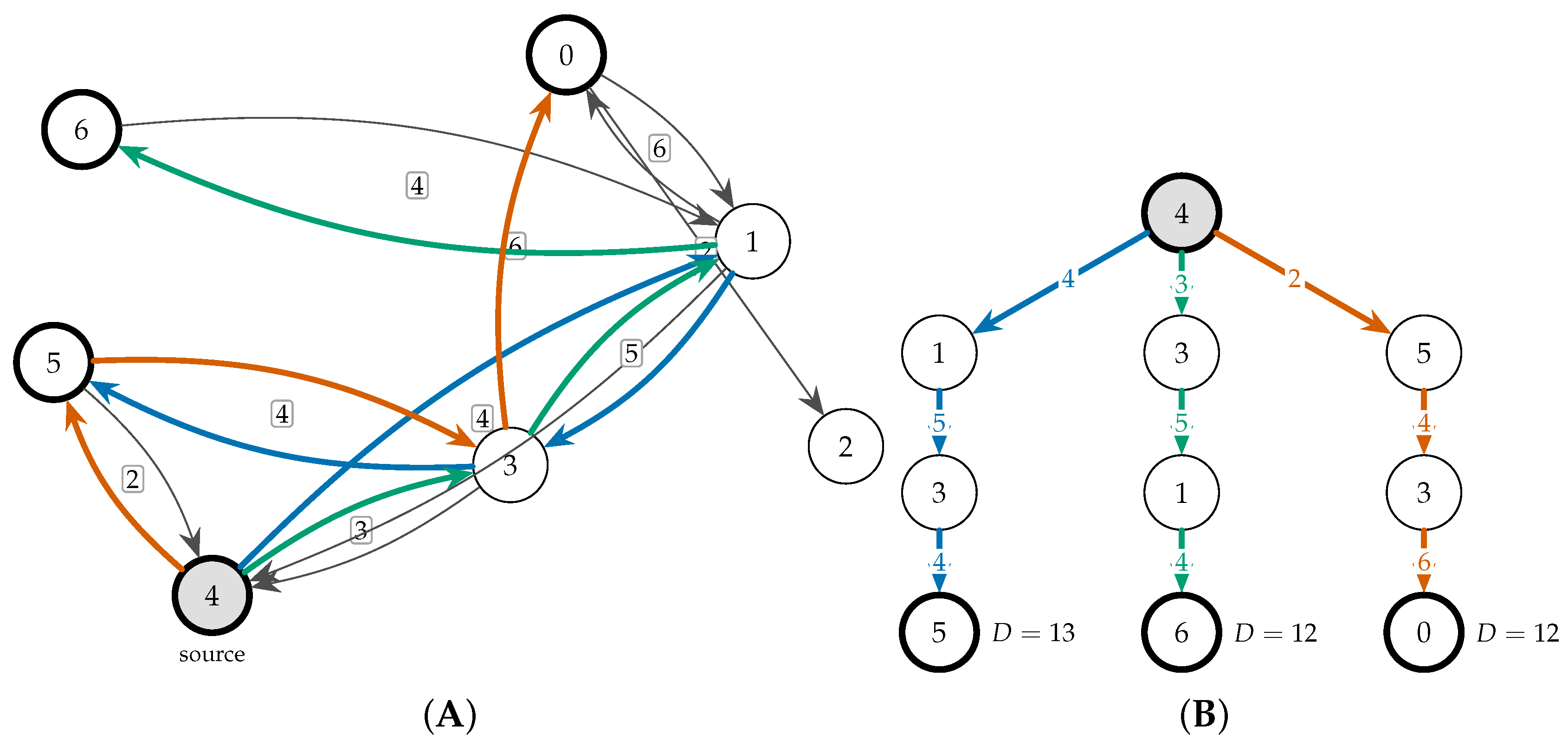Figure 1 presents both a spider-based hierarchy and a more general tree-based hierarchy. Node labels correspond to those in the topology graph.

In certain instances, the set of paths comprising a spider structure can be reconfigured into a tree. These transformations can result in trees that exhibit reduced communication costs. The following properties introduce simplifications that facilitate the development of efficient solutions.

For a routing structure X delivering delays ${\left\{d_m\right\}}_{m\in M}$ to the destinations, define the inter-destination delay variation as $\mathrm{var}\left(X\right)={max}_{m,n\in M}|d_m-d_n|$.

Proposition 1

(Dominance of hierarchies over trees, with strict separation on a bottleneck-instance family). Let $G=(V,A)$ be a directed network with non-negative arc delays, $s\in V$ the source, $M\subset V\setminus \left\{s\right\}$ the destination set, ${\mathcal{F}}_T(\Delta ,\delta )$ the set of feasible partial spanning trees, and ${\mathcal{F}}_H(\Delta ,\delta )$ the set of feasible partial spanning hierarchies, both subject to the delay bound Δ and the variation bound δ. Write ${\delta }_T^{*}={min}_{T\in {\mathcal{F}}_T}\mathrm{var}\left(T\right)$ and ${\delta }_H^{*}={min}_{H\in {\mathcal{F}}_H}\mathrm{var}\left(H\right)$ for the optimal inter-destination delay variations achievable under each structure (with the convention ${\delta }^{*}=+\infty$ when the feasible set is empty). Then:

(i) 

${\mathcal{F}}_T(\Delta ,\delta )\subseteq {\mathcal{F}}_H(\Delta ,\delta )$ for all $\Delta ,\delta \ge 0$; consequently ${\delta }_H^{*}\le {\delta }_T^{*}$ whenever a feasible tree exists.

(ii) 

There exist instances and bounds $(\Delta ,\delta )$ for which ${\mathcal{F}}_T(\Delta ,\delta )=\varnothing$ while ${\mathcal{F}}_H(\Delta ,\delta )\ne \varnothing$; that is, the inclusion in (i) can be strict.

(iii) 

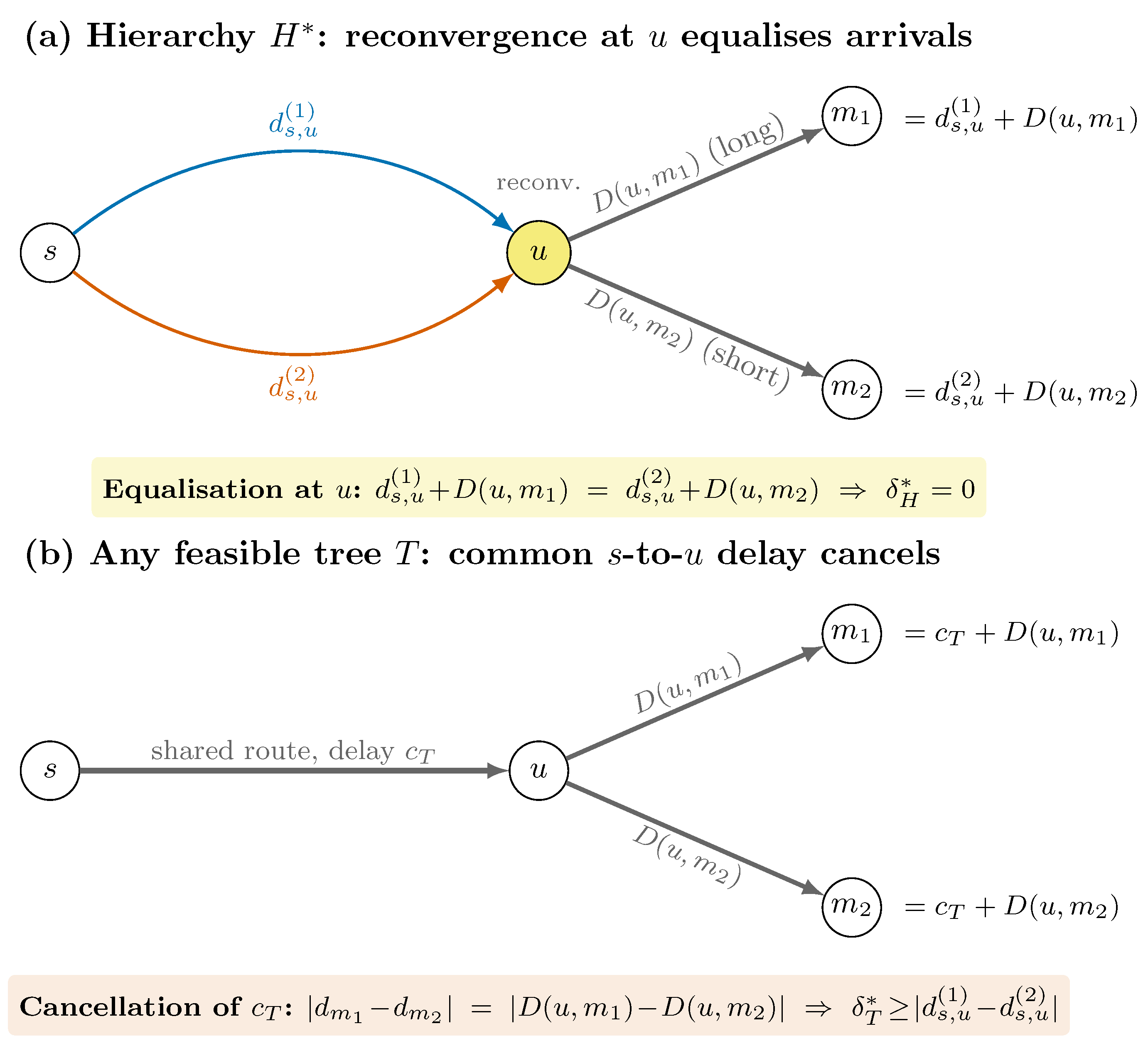
Let $H^{*}$ be a hierarchy-optimal solution and let u be a node (illustrated in Figure 1) at which two destination flows $m_1,m_2\in M$ reach u along sub-paths with distinct delays $d_{s,u}^{\left(1\right)}\ne d_{s,u}^{\left(2\right)}$ before sharing a common downstream continuation (a reconvergence node of $H^{*}$). If every feasible tree must route $m_1$ and $m_2$ through a single common sub-path to their last common ancestor at or before u, and the paths from u to the two destinations remain identical in both the tree and $H^{*}$ (so that only the route from s to u may differ), and $H^{*}$ equalizes the two arrival times at the reconvergence, i.e.,

$$d_{s,u}^{\left(1\right)}+D(u,m_1)=d_{s,u}^{\left(2\right)}+D(u,m_2)$$

(i.e., the hierarchy’s differing s-to-u delays offset the downstream imbalance), then

$${\delta }_T^{*}\ge \left|d_{s,u}^{\left(1\right)}-d_{s,u}^{\left(2\right)}\right|,\mathit{hence}{\delta }_T^{*}-{\delta }_H^{*}\ge \epsilon ,\epsilon =\left|d_{s,u}^{\left(1\right)}-d_{s,u}^{\left(2\right)}\right|-\delta .$$

(6)

In particular, whenever $\left|d_{s,u}^{\left(1\right)}-d_{s,u}^{\left(2\right)}\right|>\delta$ we have $\epsilon >0$, so the hierarchy optimum is strictly better than any feasible tree.

Proof. 

(i) Any multicast tree $T=(V_T,A_T)$ is a hierarchy under the identity homomorphism $h\left(p\right)=p$ for all $p\in V_T$; the delay of each source-to-destination path is unchanged, so T satisfies the same delay and variation bounds as a hierarchy. Hence, ${\mathcal{F}}_T\subseteq {\mathcal{F}}_H$, and minimizing the same objective over a superset cannot increase the optimum, giving ${\delta }_H^{*}\le {\delta }_T^{*}$.

(ii) (Constructive instance.) Let G contain a bottleneck arc $(u,v)$ through which every source-to-destination path must pass, and two arc-disjoint sub-paths $P_{s,u}^{\left(1\right)}$ and $P_{s,u}^{\left(2\right)}$ from s to u with delays $d_1<d_2$ and $d_2-d_1>\delta$. Choose $\Delta \ge d_2+D(u,v)+{max}_{m\in M}D(v,m)$ so that the delay bound is not binding. Consider two destinations $m_1,m_2$ whose only routing freedom is the choice of sub-path to u.

No feasible tree. In a tree, every node has a unique predecessor, so $m_1$ and $m_2$ share a single path from s to their last common ancestor ℓ. Because $(u,v)$ is a common bottleneck for both destinations, ℓ lies on the s–u portion of the tree, i.e., at or before u. Thus, both destinations inherit the same delay from s to ℓ, and the only delays available from s to u are $d_1$ and $d_2$, which are identical for both. Let $D(u,m_1)$ and $D(u,m_2)$ be the (fixed) downstream delays from u to the two destinations, and construct the instance so that $D(u,m_1)-D(u,m_2)=d_2-d_1>\delta$ (the destination reached by the faster s-to-u sub-path carries the longer downstream segment). Since the tree assigns both destinations the same s-to-u delay, that common term cancels in the inter-destination variation, which therefore equals the downstream imbalance $|D(u,m_1)-D(u,m_2)|>\delta$ regardless of whether both flows use $d_1$ or both use $d_2$. Hence no tree meets the variation bound: ${\mathcal{F}}_T(\Delta ,\delta )=\varnothing$.

A feasible hierarchy exists. The hierarchy routes $m_1$ via $P_{s,u}^{\left(1\right)}$ and $m_2$ via $P_{s,u}^{\left(2\right)}$, two independent walks that reconverge at u. Their delays to u differ by $d_2-d_1$, which by construction equals the downstream imbalance; consequently, the realized end-to-end delays $d_1+D(u,m_1)$ and $d_2+D(u,m_2)$ coincide, and the inter-destination variation is $0\le \delta$. Hence ${\mathcal{F}}_H(\Delta ,\delta )\ne \varnothing$.

Worked instance. Take $d_1=2$ and $d_2=6$ (so $d_2-d_1=4$), downstream delays $D(u,m_1)=5$ and $D(u,m_2)=1$ (downstream imbalance $|5-1|=4$), variation bound $\delta =1$, and delay bound $\Delta =8$. Every tree forces a common s-to-u delay, yielding destination delays $(2+5,2+1)=(7,3)$ or $(6+5,6+1)=(11,7)$—inter-destination variation $4>\delta$ in both cases (and $11>\Delta$ in the second)—so ${\mathcal{F}}_T=\varnothing$. The hierarchy routes $m_1$ over $P_{s,u}^{\left(1\right)}$ and $m_2$ over $P_{s,u}^{\left(2\right)}$, giving delays $2+5=7$ and $6+1=7$: variation $0\le \delta$ with both delays within $\Delta$, so ${\mathcal{F}}_H\ne \varnothing$. This witnesses the strict inclusion of part (ii).

The bottleneck-and-hub geometry underlying this construction is not a pathological worst case. It recurs in operational backbones with degree-heterogeneous routing hubs (as characterized in Topology Zoo [38]) and is instantiated by the Seattle→Chicago (or Denver) transit, through which every eastward destination in the Abilene backbone must pass (Section 5.4). The tree optimum is pinned at ${\delta }_T^{*}=6.393$ ms across every $\Delta$. The construction of part (ii) is therefore an exact description of a common real-network mechanism, not a theoretical worst case, and part (iii) quantifies the gap that this mechanism induces.

(iii) The derivation proceeds in four explicit steps that make the role of the equalization hypothesis operative (cf. Figure 2).

Step 1 (tree structure forces a common upstream delay). By hypothesis, in any feasible tree T the destinations $m_1,m_2$ traverse a single common sub-path from s to their last common ancestor, which lies at or before u, and only the route from s to u may differ from $H^{*}$. Hence both destinations receive the same s-to-u delay in T; call it $c_T$ (whatever route T selects).

Step 2 (tree delays and cancellation). Because the downstream segments from u are fixed and identical in T and $H^{*}$, the realized tree delays are $d_{m_1}\left(T\right)=c_T+D(u,m_1)$ and $d_{m_2}\left(T\right)=c_T+D(u,m_2)$, so

$$\left|d_{m_1}\left(T\right)-d_{m_2}\left(T\right)\right|=\left|D(u,m_1)-D(u,m_2)\right|,$$

in which the common upstream term $c_T$ cancels. This is the precise reason the tree cannot compensate through the downstream segments: those segments are fixed by hypothesis, and $c_T$, the only quantity the tree controls, enters both delays identically and therefore has no effect on their difference.

Step 3 (identifying the downstream imbalance via the equalization hypothesis). By the equalization hypothesis on $H^{*}$, $d_{s,u}^{\left(1\right)}+D(u,m_1)=d_{s,u}^{\left(2\right)}+D(u,m_2)$; rearranging gives

$$\left|D(u,m_1)-D(u,m_2)\right|=\left|d_{s,u}^{\left(1\right)}-d_{s,u}^{\left(2\right)}\right|.$$

Substituting this into Step 2 yields $\left|d_{m_1}\left(T\right)-d_{m_2}\left(T\right)\right|=\left|d_{s,u}^{\left(1\right)}-d_{s,u}^{\left(2\right)}\right|$ for every feasible tree.

Step 4 (conclusion). Since the tree variation is at least the pairwise difference just derived, $\mathrm{var}\left(T\right)\ge \left|d_{s,u}^{\left(1\right)}-d_{s,u}^{\left(2\right)}\right|$, and therefore ${\delta }_T^{*}\ge \left|d_{s,u}^{\left(1\right)}-d_{s,u}^{\left(2\right)}\right|$, which is Inequality (6). Because $H^{*}$ is feasible, ${\delta }_H^{*}\le \delta$; subtracting the two bounds yields ${\delta }_T^{*}-{\delta }_H^{*}\ge \left|d_{s,u}^{\left(1\right)}-d_{s,u}^{\left(2\right)}\right|-\delta =\epsilon$, strictly positive whenever $\left|d_{s,u}^{\left(1\right)}-d_{s,u}^{\left(2\right)}\right|>\delta$. □

Corollary 1.

(a) Omitting the single-predecessor constraint (17) from any ILP in Section 4 enlarges the feasible region, and strictly so whenever the instance satisfies the hypothesis of part (ii) (${\mathcal{F}}_T(\Delta ,\delta )=\varnothing$, ${\mathcal{F}}_H(\Delta ,\delta )\ne \varnothing$). (b) Under the hypothesis of part (iii), the ILP-hierarchy optimum attains variation ${\delta }_H^{*}\le \delta$, whereas every multicast tree—and therefore every tree-restricted heuristic—attains variation at least ${\delta }_T^{*}\ge {\delta }_H^{*}+\epsilon$. Hence no tree-restricted method can come within ε of the hierarchy optimum, irrespective of the heuristic’s sophistication.

Remark 1

(Scope of Proposition 1(iii)). The hypothesis of part (iii)—that every feasible tree must route $m_1$ and $m_2$ through a single common sub-path to their last common ancestor at or before the reconvergence node u—is a sufficient condition for a strict gap between hierarchies and trees, not a necessary one. When this structural obstruction is absent (e.g., when the topology offers multiple paths of equal delay that allow a tree to replicate the hierarchy’s equalization), hierarchies and trees may achieve equal variation for specific bounds. Part (ii) establishes that strict inclusion of the feasible regions exists for some instances; part (iii) quantifies the gap when the sufficient condition is met. Neither part claims that hierarchies always strictly beat trees. The empirical incidence of the two regimes is characterized in Section 5.3: on 120 proven-optimal random instances, the strict gap holds in $95–98\%$ of cases, and the residual near-zero tail is exactly the conditional-tie regime delimited above.

Two complementary structural features drive a substantive (non-cosmetic) gap. (a) Bottleneck reconvergence: Whenever an instance shows the bottleneck structure of part (ii)—a shared bottleneck arc reachable via delay-heterogeneous alternative sub-paths, along with an unequal downstream imbalance from that bottleneck to the destinations — a tree must accept the raw downstream imbalance as its variation floor. A hierarchy can offset it exactly (Proposition 1(ii)–(iii)). Bottleneck-and-hub patterns like this are characteristic of real backbone topologies with degree-heterogeneous routing hubs [38], not pathological constructions. The Abilene backbone in Section 5.4, where the tree optimum is pinned at ${\delta }_T^{*}=6.393$ ms across every $\Delta$ while the hierarchy reduces variation by 78–$99\%$, is an operational example.

(b) Large SPT spread: On 120 random Erdős–Rényi instances (Section 5.3), the median proven-optimal reduction $({\delta }_T^{*}-{\delta }_H^{*})/{\delta }_T^{*}$ is 86–$92\%$ and strictly positive on 95–$98\%$ of instances. The near-zero tail is exactly Remark 1’s conditional-tie regime. The density sweep shows the tree variation floor rising as sparsity increases, consistent with the gap narrowing at higher density. Together, these give an operational answer: the improvement is cosmetic on dense graphs with abundant near-equal alternative paths and substantial in the sparse, delay-heterogeneous regime that dominates real backbones.

Observation 1.

Let $W_1$ and $W_2$ be two walks from the source s and terminating at destinations x and y, respectively. Let a and b be nodes common to both walks. Denote by $w_1(a,b)$ and $w_2(a,b)$ the sub-walks between a and b on $W_1$ and $W_2$, respectively. Assume that $D\left(w_1(a,b)\right)=D\left(w_2(a,b)\right)$, meaning the delays between nodes a and b on $W_1$ and $W_2$ are equal. Under these conditions, either sub-walk may replace the other without altering the endpoint delays or the delay variation.

Proof. 

This property is demonstrated for walk $W_1$; the argument for other walks is analogous. Let $D\left(W_1\right)$ denote the delay on walk $W_1$, and let $\widetilde{D\left(W_1\right)}$ represent the delay on $W_1$ excluding the sub-walk $w_1(a,b)$. Thus, $D\left(W_1\right)=\widetilde{D\left(W_1\right)}+D\left(w_1(a,b)\right)=\widetilde{D\left(W_1\right)}+D\left(w_2(a,b)\right)$. Therefore, replacing $w_1(a,b)$ with $w_2(a,b)$ does not affect the delay at the endpoint or the delay variation. □

These simplifications remain valid when substituting one sub-walk for another results in only a minor change to the end-to-end delay, provided that the constraints defined by $\Delta$ and $\delta$ are not violated. This property can be generalized as follows. Let $W_m$ and $W_M$ represent the walks with minimal and maximal delays, respectively. If $D\left(W_m\right)\le \widetilde{D\left(W_1\right)}+D\left(w_2(a,b)\right)\le D\left(W_M\right)$, then replacing $w_1(a,b)$ with $w_2(a,b)$ is permissible without violating the specified constraints. 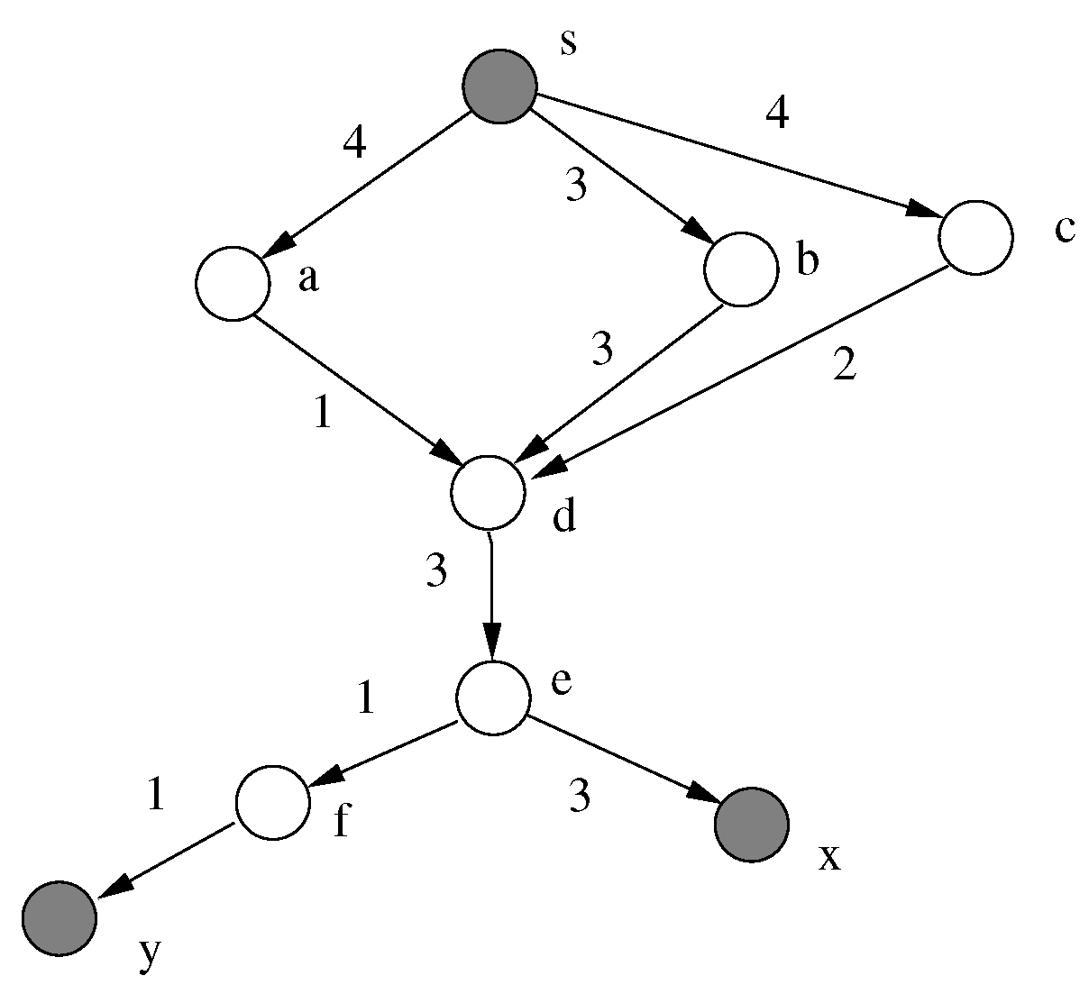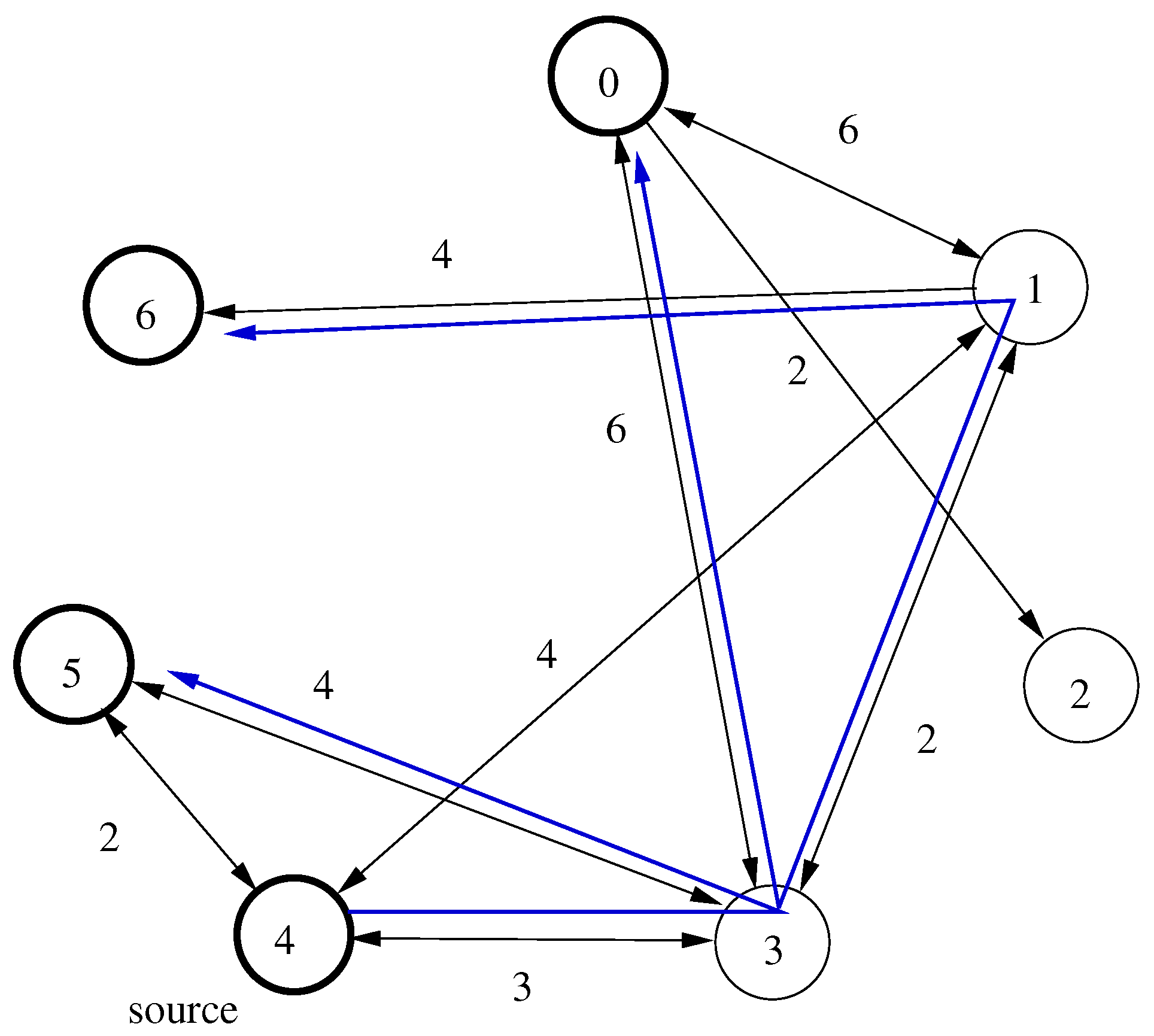Figure 3 presents a simple network. In this network, $D(s,b,d)=D(s,c,d)$. Either sub-walk $(s,b,d)$ or $(s,c,d)$ can be substituted for the other.

Sharing arcs among different walks can substantially reduce communication costs. Multicast trees illustrate the cost reductions achievable through arc sharing. When an arc is shared by two walks leading to distinct destinations, the message from the source traverses this arc only once, benefiting both destinations. The following property establishes a sufficient condition for arc sharing in group communication scenarios.

Observation 2.

Let $W_1$ and $W_2$ be two walks with a common prefix between s and a. Let x and y be their respective endpoints. The common prefix can be shared, yielding a new hierarchy without changing endpoint delays or delay variation.

Proof. 

Before sharing, the tree T in the hierarchy $H=(T,G,h)$ connecting s to the endpoints x and y is a spider. Let $T^{\prime }$ be the directed tree containing the common prefix $(s,a)$ of both paths and the remaining paths from a to x and y respectively. The hierarchy contains the two original walks in G, and the delays remain unchanged. Concretely, sharing the prefix leaves each source-to-endpoint delay equal to $D(s,a)$ plus the unchanged suffix delay $D(a,x)$ or $D(a,y)$; since neither term is altered, both endpoint delays—and hence the variation—are invariant. □

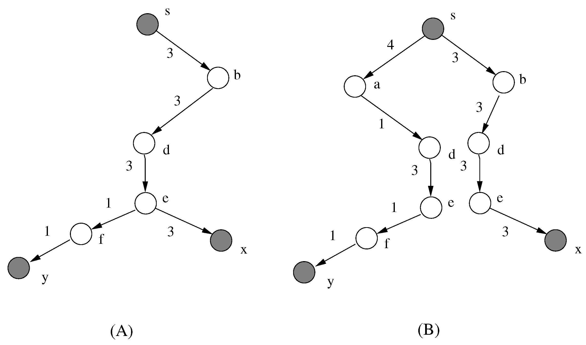
Consider the solution consisting of walks $(s,b,d,e,x)$ to destination x and $(s,b,d,e,f,y)$ to y in Figure 3. The prefix $(s,b,d,e)$ can be shared; see Figure 4A for the resulting tree $T^{\prime }$ after sharing. In general, an arbitrary common sub-walk that is not a prefix cannot necessarily be shared. For example, in the solution consisting of walks $(s,a,d,e,x)$ and $(s,b,d,e,f,y)$, the arc $(d,e)$ is common but cannot be shared. Figure 4B illustrates the correct non-sharing solution.

4. Exact ILP Formulations for Fairness-Aware Routing

Section 2.3 identifies three principal modeling approaches for fair routing:

• Finding a feasible solution;
• Using a multi-objective optimization;
• Using a multi-constrained optimization.

This section explicitly formulates different versions of the optimal fairness routing problem using linear optimization techniques. These formulations address trade-offs between performance objectives and network feasibility constraints. A digraph $G=(V,A)$ representing the network topology is used to facilitate computation. Flows are determined from a single source s to destination nodes defined by the set M. The resulting solution is a valued, directed subgraph of the original network topology. The mathematical formulation employs three types of decision variables to describe arc occurrences, flows, and shared usage between flows. These variables are formally defined in Table 1.

For a network with $\left|V\right|$ nodes, $\left|A\right|$ arcs, and $\left|M\right|$ destinations, the ILP has $O\left(\right|A|·|M{|}^2+\left|A\right|)$ variables and $O\left(\right|V|·|M|+|A\left|\right)$ constraints. The dominant constraint family is the per-destination flow conservation (Equations (20) and (21)), which scales as $O\left(\right|V|·|M\left|\right)$. The arc-sharing constraints (Equations (24)–(27)) introduce $O\left(\right|A|·|M{|}^2)$ continuous sharing variables. Only the $\left|M\right|·\left|A\right|$ flow variables $F(m,a)$ are declared integer; $x\left(a\right)$ and $\sigma (m,n,a)$ are continuous and pinned to integer values by the linearization constraints, so the branch-and-bound tree branches only on F. Let $d_m\triangleq {\sum }_{a\in A}F(m,a)·D\left(a\right)$ denote the end-to-end delay to destination $m\in M$. The proposed linear optimization formulations incorporate the following objective functions to address fairness and performance in multicast routing.

• Objective Functions

(OF1) Minimum overall network cost:

$$min\sum _{a\in A}x\left(a\right)·C\left(a\right)$$

(7)

where $C\left(a\right)$ is the cost of arc $a\in A$, minimizing the total cost incurred by arc occurrences across the multicast hierarchy.

(OF2) Minimum end-to-end delays:

$$min\sum _{m\in M}{d}_m.$$

(8)

The interpretation of OF2 differs sharply between its single-objective and multi-objective uses, and we make the distinction explicit here to prevent the decomposition claim below from being read as a general property of every scenario in

Table 2. Representative linear programming-based optimization scenarios.

Optimization Type	Problem Description	Objective Function(s)	Constraints
Multi-objective optimization	Minimization of costs, delays, and variation	Equations (7), (8) and (12)	Equations (15)–(23)
Multi-objective optimization	Minimization of delays and variation	Equations (8) and (12)	Equations (15)–(27)
Multi-constrained optimization	Minimization of costs	Equations (7)	Equations (13), (14), (16)–(27)
Multi-constrained optimization	Minimization of delays	Equations (8) or (11)	Equations (13), (14), (16)–(27)
Multi-constrained optimization	Multi-constrained Steiner tree construction	Equations (7)	Equations (13), (14), (16)–(23)

.

Single-objective use. When OF2 is the sole objective, the per-destination delays ${\left(d_m\right)}_{m\in M}$ are mutually independent: each $d_m$ depends only on the route serving destination m and is unaffected by the routes to the other destinations. The problem therefore decomposes into $\left|M\right|$ independent shortest-path computations, and every monotone aggregation of the delay vector (sum, maximum, leximin) is optimized by the same routes, so no scalarization choice arises. In an undirected graph, this optimum is the delay-shortest-path tree (SPT); in a directed graph, it is a set of directed shortest paths that form a spider-based spanning hierarchy in which the destination delays are independently minimal. In this regime, the ILP machinery is not required.

Multi-objective use. The decomposition holds only in isolation. As soon as OF2 is combined with the cost objective (7) or with the variation objective (10)–(12) in a row of Table 2, the shared arc-usage variable $x\left(a\right)$ and the pairwise sharing variable $\sigma (m,n,a)$ couple the destinations, a genuine trade-off appears, and the delays can no longer be optimized independently. In every multi-objective row of Table 2, OF2 denotes the aggregate form (8) as one component of a Pareto or scalarized problem, not an independently attainable optimum. No other objective in the paper, in particular OF4 (12)—enjoys such a decomposition, so the reader should not extend the “independent shortest paths” reading to those rows.

(OF3) Minimum maximum end-to-end delay:

$$min\underset{m\in M}{max}{d}_m$$

(9)

This ensures responsiveness by targeting the path with the greatest delay.

(OF4) Minimum inter-destination delay variation:

$$min\underset{m,n\in M}{max}|d_m-d_n|$$

(10)

This reduces the maximum pairwise delay difference across destinations $m,n\in M$, promoting synchronized message reception.

Epigraph linearization of the min–max objectives. Objectives (9) and (10) are not linear as written; both are recast in mixed-integer linear form by the standard epigraph technique. For OF3, introduce a continuous variable $z_{max}$ and replace (9) by

$$min{z}_{max}\mathrm{s}.\mathrm{t}.z_{max}\ge d_m,\forall m\in M.$$

(11)

For OF4, introduce a continuous variable $z_{\mathrm{var}}$ and replace (10) by

$$min{z}_{\mathrm{var}}\mathrm{s}.\mathrm{t}.z_{\mathrm{var}}\ge d_m-d_n,z_{\mathrm{var}}\ge d_n-d_m,\forall m,n\in M.$$

(12)

At optimality $z_{max}={max}_m{d}_m$ and $z_{\mathrm{var}}={max}_{m,n}|d_m-d_n|$, so both reformulations are exact. Together with the McCormick/big-M linearization of the sharing products below, every scenario in Table 2 is a genuine integer linear program.

The following constraints ensure compliance with delay limits, fairness conditions, and structural feasibility of the multicast solution.

• End-to-end delay constraint.

$$d_m\le \Delta ,\forall m\in M\left(\mathrm{equivalently}:\underset{m\in M}{max}{d}_m\le \Delta \right)$$

(13)

• Delay-variation constraint.

$$|d_m-d_n|\le \delta ,\forall m,n\in M\left(\mathrm{equivalently}:\underset{m,n\in M}{max}|d_m-d_n|\le \delta \right)$$

(14)

• Structural constraints on arcs.

• No incoming arcs to the source:

  $$x\left(a\right)=0,\forall a\in \mathrm{In}\left(s\right)$$

  (15)
• Each destination node must have a predecessor:

  $$\sum _{a\in \mathrm{In}\left(m\right)}x\left(a\right)\ge 1,\forall m\in M$$

  (16)
• Tree structure (single predecessor per node):

$$\sum _{a\in \mathrm{In}\left(v\right)}x\left(a\right)\le 1,\forall v\in V$$

(17)

For a partial spanning tree (e.g., constrained Steiner tree), each node is restricted to a single predecessor in the solution.

• Flow Conservation and Connectivity.
• No flow returns to the source:

  $$\sum _{m\in M}\sum _{a\in \mathrm{In}\left(s\right)}F(m,a)=0$$

  (18)
• Unit flow dispatched from source to each destination:

  $$\sum _{a\in \mathrm{Out}\left(s\right)}F(m,a)=1,\forall m\in M$$

  (19)
• Flow conservation at each destination:

  $$\sum _{a\in \mathrm{Out}\left(m\right)}F(m,a)=\sum _{a\in \mathrm{In}\left(m\right)}F(m,a)-1,\forall m\in M$$

  (20)
• Flow conservation at intermediate nodes:

  $$\sum _{a\in \mathrm{Out}\left(v\right)}F(m,a)=\sum _{a\in \mathrm{In}\left(v\right)}F(m,a),\forall v\in V\setminus \left\{s\right\}\setminus \left\{m\right\},\forall m\in M$$

  (21)

• Arc-Usage linearization.

• Arc usage (lower bound):

  $$x\left(a\right)\ge F(m,a),\forall m\in M,\forall a\in A$$

  (22)
• Arc usage (upper bound):

  $$x\left(a\right)\le \sum _{m\in M}F(m,a),\forall a\in A$$

  (23)

Equations (22) and (23) together linearize $x\left(a\right)={max}_{m\in M}F(m,a)$ for binary F: the lower bound forces $x\left(a\right)\ge 1$ whenever some flow uses a, and the upper bound forces $x\left(a\right)=0$ whenever no flow does. The linearization is objective-agnostic; in particular, it does not rely on x appearing in a cost term, so it remains tight under objectives that omit ${\sum }_{a}x\left(a\right)·C\left(a\right)$, including OF3 (11) and OF4 (12). Because F is binary, $x\left(a\right)$ is automatically in $\{0,1\}$, so integrality need not be declared.

• Validity of the delivery structure.

Together, Equations (15)–(23) enforce all requirements of a valid multicast delivery structure.

• Flow conservation.

A unit of flow is dispatched from the source for each destination m (19) and absorbed at that destination (20). Balance is preserved at every intermediate node (21), and no flow returns to the source (18).

• Destination reachability.

Because the per-destination flow of unit magnitude cannot vanish under conservation, every destination is connected to the source by at least one directed walk of active arcs (22). Thus, the projection $G_H=(V,\{a:x\left(a\right)=1\})$ contains an s-to-m walk for every $m\in M$.

• Path consistency.

Each destination flow is an integer s-to-m unit flow on the arc set ((19)–(21)). By the flow-decomposition theorem, this is realizable as a single directed walk from s to m. This walk is an elementary path if acyclic; otherwise, its homomorphic image is the tree used in Definition 1.

• Reconvergent routes are always feasible, not infeasible.

Reconvergence in a hierarchy, where two destination flows share a downstream continuation after distinct upstream sub-paths, is precisely the mechanism analyzed in Proposition 1(iii). It is admitted by construction whenever the single-predecessor constraint (17) is omitted, and forbidden when (17) is imposed. The formulation therefore does not need to detect and exclude infeasible reconvergent routes. Every reconvergent structure that respects flow conservation is a valid hierarchy in the sense of Definition 1. Adding (17) recovers the strict tree regime as a special case.

• Arc-Sharing Constraints.

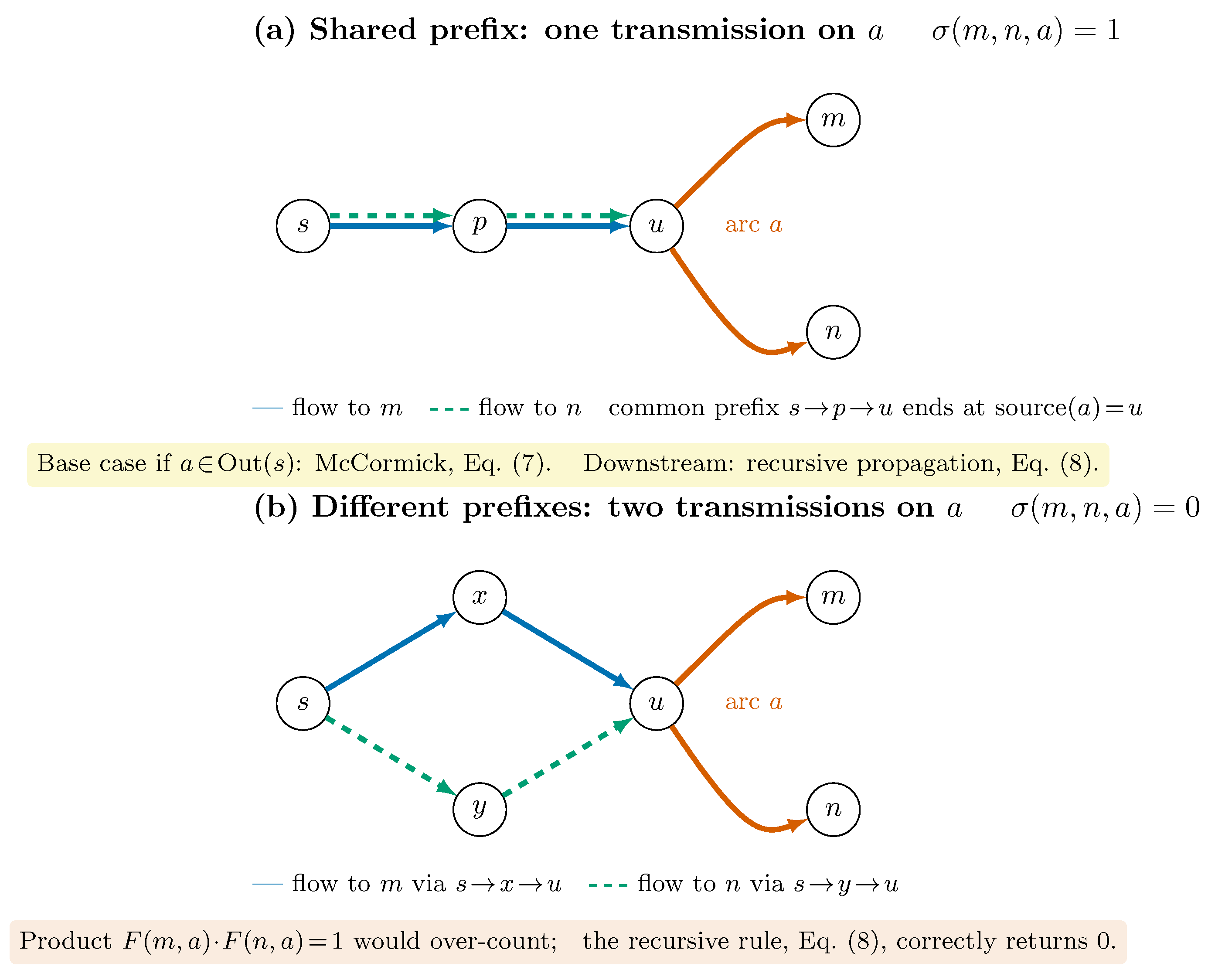
The sharing variable $\sigma (m,n,a)\in [0,1]$ is defined by two cases, because the semantics of “a single transmission serves both destinations” requires the two flows to arrive at $\mathrm{source}\left(a\right)$ along a common shared prefix. Two flows may traverse the same downstream arc after arriving along different (unshared) prefixes; in that case the message is transmitted twice on the arc, and the arc is not shared. The product $F(m,a)·F(n,a)$ would incorrectly label such coincidental joint usage as sharing, so it is used only where the two coincide (Figure 5).

• Base case—source outgoing arcs $a\in \mathrm{Out}\left(s\right)$.

Every flow originates at s, so joint usage and prefix-sharing coincide: here $\sigma (m,n,a)=F(m,a)·F(n,a)$ exactly, linearized by the three McCormick inequalities (24).

• Recursive case—all other arcs $a\notin \mathrm{Out}\left(s\right)$.

$\sigma (m,n,a)=1$ iff both flows traverse a and share a common prefix ending at $\mathrm{source}\left(a\right)$. Sharing is propagated along such prefixes by the recursive lower bound (26) and pinned to zero on non-shared prefixes by the downstream upper bound (27). Applying the lower-bound inequality $\sigma \ge F(m,a)+F(n,a)-1$ of (24) to these arcs would over-constrain the model by labeling coincidental joint usage as sharing.

• Direct sharing at source outgoing arcs (base case).

For $a\in \mathrm{Out}\left(s\right)$, joint usage and prefix-sharing coincide, so $\sigma (m,n,a)=F(m,a)·F(n,a)$. For binary F this is linearized by the standard three McCormick inequalities:

$$\begin{array}{cc}\hfill \sigma (m,n,a)& \le F(m,a),\hfill \\ \hfill \sigma (m,n,a)& \le F(n,a),\hfill \\ \hfill \sigma (m,n,a)& \ge F(m,a)+F(n,a)-1,a\in \mathrm{Out}\left(s\right).\hfill \end{array}$$

(24)

• Global validity upper bound.

An arc that a flow does not use cannot be shared by it, so on every arc:

$$\sigma (m,n,a)\le F(m,a),\sigma (m,n,a)\le F(n,a),\forall a\in A,\forall m,n\in M.$$

(25)

• Sharing propagated via incoming arcs (recursive lower bound).

$$\sigma (m,n,a)\ge \sigma (m,n,b)+F(m,a)+F(n,a)-2,\forall a\in A\setminus \mathrm{Out}\left(s\right),\forall b\in \mathrm{In}\left(\mathrm{source}\right(a\left)\right).$$

(26)

• Sharing propagated via incoming arcs (downstream upper bound).

On non-source arcs, sharing can propagate onto a only if some incoming arc into $\mathrm{source}\left(a\right)$ already carries a shared prefix:

$$\sigma (m,n,a)\le \sum _{b\in \mathrm{In}\left(\mathrm{source}\right(a\left)\right)}\sigma (m,n,b),\forall a\in A\setminus \mathrm{Out}\left(s\right),\forall m,n\in M.$$

(27)

Equations (24)–(27) together pin $\sigma (m,n,a)$ to the two-case semantics of Figure 5 on every arc. Specifically: on $a\in \mathrm{Out}\left(s\right)$, the McCormick system (24) sets $\sigma (m,n,a)=F(m,a)·F(n,a)$. On $a\notin \mathrm{Out}\left(s\right)$, three cases arise. (i) If either flow does not use a, the global upper bound (25) forces $\sigma (m,n,a)=0$. (ii) If both flows use a but no incoming arc into $\mathrm{source}\left(a\right)$ carries a shared prefix, the downstream upper bound (27) forces $\sigma (m,n,a)=0$; this is the “coincidental joint usage” case of Figure 5 (bottom). (iii) If both flows use a and some incoming arc carries a shared prefix, the recursive lower bound (26) forces $\sigma (m,n,a)\ge 1$, and the global upper bound caps it at 1. Because F is binary, $\sigma$ is automatically in $\{0,1\}$ on every arc, so integrality need not be declared.

The combination of these objective functions and constraints enables the formulation of various optimization scenarios addressing distinct fairness and efficiency requirements. Table 2 presents representative cases.

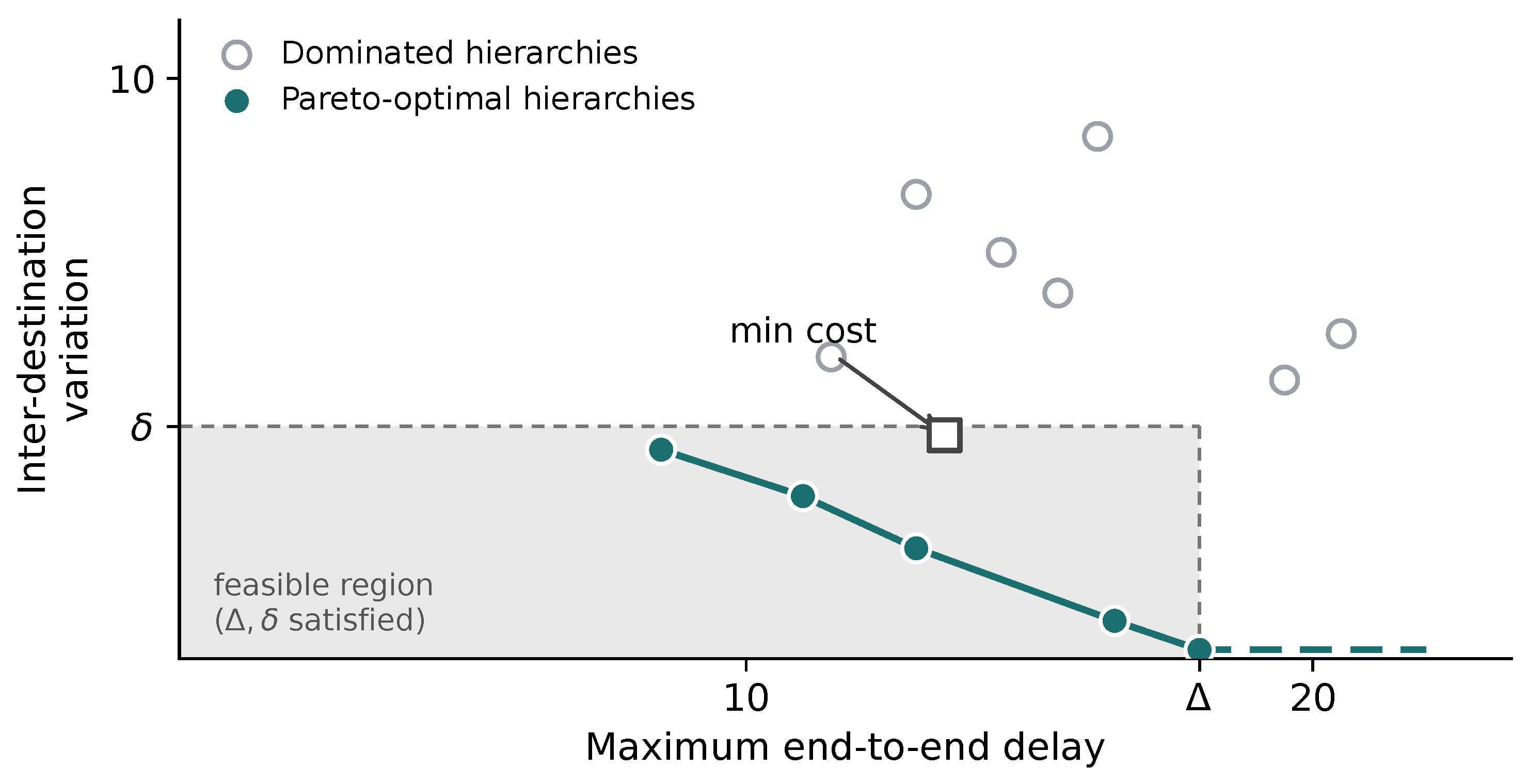
Figure 6 presents example solutions for a multicast group within a network. Each circle denotes a hierarchy, or multicast subgraph, connecting the source to all destination nodes. Each hierarchy is characterized by its maximum delay and inter-destination delay variation. The figure shows the Pareto front for the delay and variation objectives. The rectangle defined by $\Delta$ and $\delta$ represents the feasible region that satisfies the corresponding constraints. Although each hierarchy carries an associated cost, only the cost-optimal hierarchy is explicitly marked in the plot; the full $(\delta ,\Delta ,\mathrm{cost})$ triples for every point are available in the paper’s public repository. It is important to note that the cost-optimal solution does not always belong to the Pareto set of delay–delay-variation trade-offs.

• Discussion of multi-objective optimizations.

The combination of objective functions (7), (8), and (10) constitutes a genuine multi-objective integer program. Its Pareto-optimal set—the surface of trade-offs among conflicting objectives—can be computed exactly using the augmented $\epsilon$-constraint method (AUGMECON2) [39]. To maintain consistency in aggregation, the aggregation function must be strictly increasing with respect to each individual objective. Typical aggregation functions include the sum, average, minimum, or maximum of the objective values. The max–min fairness strategy, which maximizes the minimum satisfaction across all criteria, $max\{min{f}_i\left(x\right):x\in Q\},i=1,\dots ,m$, improves the worst-performing metric but may reduce the performance of others. This approach aligns with the Rawlsian maximin axiom discussed in Section 2.2. However, if one objective performs significantly worse than the others, prioritizing it can lead to an imbalanced or suboptimal trade-off.

• Discussion of Multi-Constrained Optimizations.

A solution to the original DVBMT problem may be obtained using a constrained Steiner tree formulation. If Constraint (17) is omitted, a Steiner hierarchy, which constitutes a non-tree solution, can be constructed to satisfy fairness constraints. Constrained formulations may involve minimizing delay variation subject to a fixed maximum delay, or minimizing the maximum delay subject to a fixed allowable variation. Additional Quality-of-Service (QoS) constraints, such as bandwidth limits, packet-loss thresholds, or reliability requirements, may also be incorporated to achieve more comprehensive fairness-aware group communication. These considerations, however, are beyond the scope of the present analysis.

5. Experimental Evaluation

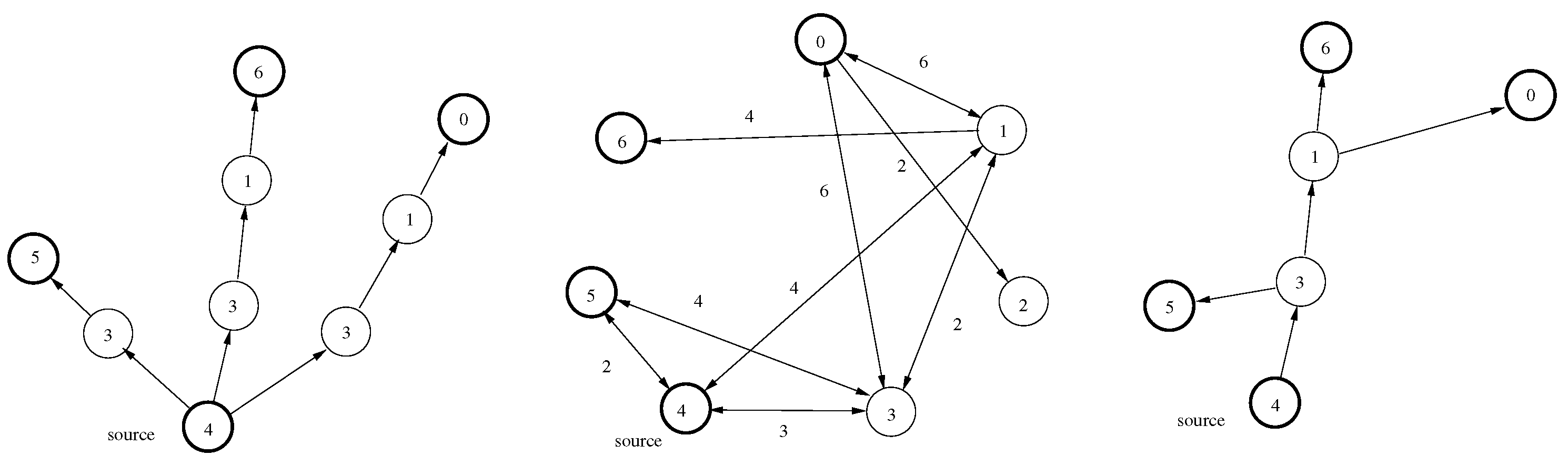
This case study examines the minimization of delay variation under bounded delay constraints. When significant delay differences exist between paths, as in shortest-path routing, delay variation can be reduced by intentionally selecting slightly longer paths for certain destinations, provided all delays remain within the specified bounds. Figure 7 presents a test network with seven nodes and 16 arcs. Arcs are represented as directed edges, with arc labels indicating transmission delays. From source node 4, destinations $\{0,5,6\}$ must receive messages within the delay bound $\Delta =13$. The hierarchical approach selects non-shortest walks that reconverge at intermediate nodes, resulting in near-equalized arrivals with variation ${\delta }^{*}=1$ (destination delays $13,12,12$).

• Instances.

Two Erdős–Rényi instances are used throughout this section; both are defined here and referenced by name thereafter. Instance I is a 12-node, 48-arc network (arc probability $p=0.35$, random seed 42; source node 10, destinations $\{0,1,3,4,6,9,11\}$, so $\left|M\right|=7$). Instance II is a larger 15-node, 64-arc network ($p=0.32$, seed 200, $\left|M\right|=8$), generated independently. Both draw arc delays and costs from continuous uniform distributions over $[2,5]$ and $[1,10]$, respectively, and all integer programs in this section are solved to proven optimality with the HiGHS solver [40].

We first analyze Instance I, which is distinct from the seven-node illustrative example above; the same delay bound $\Delta =13$ therefore yields a different optimum, ${\delta }^{*}=0.112$ here (

Table 3. Spanning hierarchies minimizing delay variation under increasing delay bounds (Instance I; HiGHS proven-optimal). Jain’s fairness index of the optimal delay vector is reported alongside the variation; $J=1$ denotes perfect equality.

Delay Bound	Variation	Jain	Average Delay	Min Delay	Max Delay	Cost	Arcs Used
7	3.778	0.9462	5.437	3.137	6.915	43	8
9	2.633	0.9819	6.298	4.998	7.631	57	9
11	2.633	0.9819	6.298	4.998	7.631	57	9
13	0.112	1.0000	12.922	12.862	12.973	140	22
15	0.059	1.0000	14.702	14.680	14.739	103	20

) versus ${\delta }^{*}=1$ for the seven-node network (Figure 7). The resulting hierarchies span the multicast group and minimize inter-destination delay variation. Table 3 presents a summary of the results.

Alongside the variation ${\delta }^{*}$, each table in this section reports Jain’s fairness index [17] of the optimal delay vector,

$$J\left(d\right)={\displaystyle \frac{{\left({\sum }_{m\in M}{d}_m\right)}^2}{\left|M\right|{\sum }_{m\in M}{d}_m^2}},{\displaystyle \frac{1}{\left|M\right|}}\le J\left(d\right)\le 1,$$

(28)

with $J\left(d\right)=1$ iff all delays are equal (perfect equalization). We emphasize that J is not an optimization objective of any ILP in this paper: it is non-linear in ${\left(d_m\right)}_{m\in M}$ and therefore ILP-intractable (cf. Section 2.4). It is computed a posteriori on the solver’s optimal delay vector, and serves as an independent fairness measure to cross-validate the ${\delta }^{*}$ ranking through a member of the Lan et al. [16] axiomatic family. This caveat also applies to Jain values reported in Table 5 and Table 8.

A comparison against published heuristics is deferred to the consolidated study of Table 5, which benchmarks the ILP optima against CHAINS [14], the strongest heuristic in this lineage. Several notable trends emerge as the delay bound increases:

• When the delay bound is less than the minimum feasible delay for any destination, constructing a valid solution is not possible.
• When the delay bound is stringent but feasible paths exist, solutions frequently exhibit significant delay variation.
• As the delay bound increases, additional alternative paths become available, which enables the construction of walks with reduced delay variation.

Imposing structural constraints on arc usage transforms the computed solution into a directed multicast tree. Specifically, revisiting previously traversed nodes is prohibited, and each node in the topology may be visited at most once. In the context of hierarchy construction, this constraint enforces an injective mapping from the nodes of the solution tree T to the nodes of the topology graph G. Since loops and multiple arc usages are disallowed, the resulting tree structure differs from that of unconstrained hierarchies. These constraints reduce the potential to construct hierarchies with minimal delay variance.

Figure 8 illustrates this effect. The multicast tree depicted achieves minimal delay variation under a delay bound of 9. In this solution, the delays experienced by destinations 5, 6, and 0 are 7, 8, and 9, respectively, resulting in a delay variation of 2. The tree spans five arcs. Although constructing a tree with only four arcs is possible, it would result in a higher delay variation.

A subsequent series of calculations produced spanning trees with minimal delay variation for the same multicast group and network topology, using the same range of delay bounds. The only distinction from the initial experiment is the addition of a structural constraint that enforces each node has at most one incoming arc (cf. Constraint 17).

Table 4. Spanning trees minimizing inter-destination delay variation under increasing delay bounds (Instance I; HiGHS proven-optimal, with Jain’s index of the optimal delay vector).

Delay Bound	Variation	Jain	Average Delay	Min Delay	Max Delay	Cost	Arcs Used
7	3.778	0.9462	5.437	3.137	6.915	43	8
9	3.601	0.9715	6.436	4.998	8.599	58	10
11	3.577	0.9756	8.160	6.883	10.459	54	10
13	3.577	0.9756	8.160	6.883	10.459	54	10
15	2.418	0.9942	13.095	12.236	14.655	54	11

presents the corresponding results.

A comparison of the hierarchy-based and tree-based solutions reveals the following:

• Spanning trees are structurally more rigid than hierarchies, which results in larger delay variations for the same delay bounds.
• However, spanning trees often exhibit smaller maximum delays than hierarchies.
• Because of fewer path options, tree-based solutions tend to have lower costs than their hierarchy-based counterparts.

5.1. Cross-Topology Quantification of the Hierarchy Gap

Since every tree is a hierarchy (Proposition 1(i)), the inequality ${\delta }_H^{*}\le {\delta }_T^{*}$ holds by construction and is not in question. The purpose of this subsection is therefore not to test dominance but to quantify the size of the gap, and to show that it remains non-trivial on a second, independently generated topology rather than being an artifact of one instance. When no feasible tree exists, ${\delta }_T^{*}=+\infty$ and the gap is unbounded. 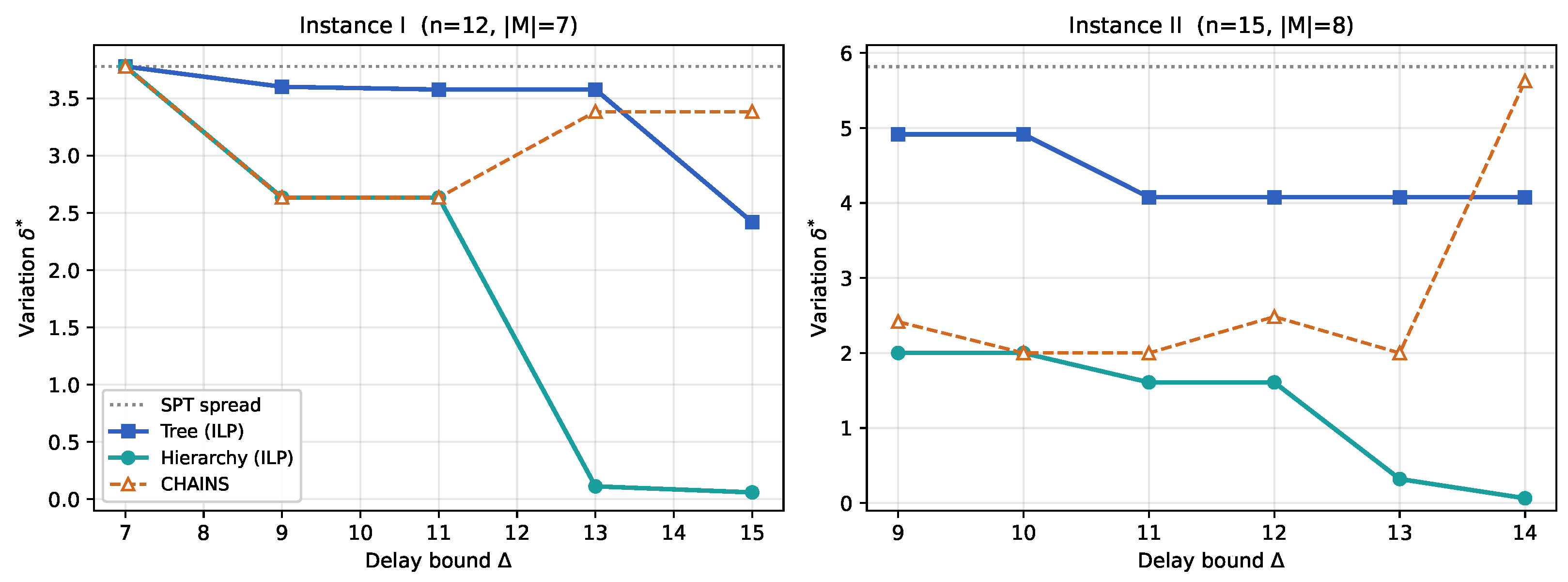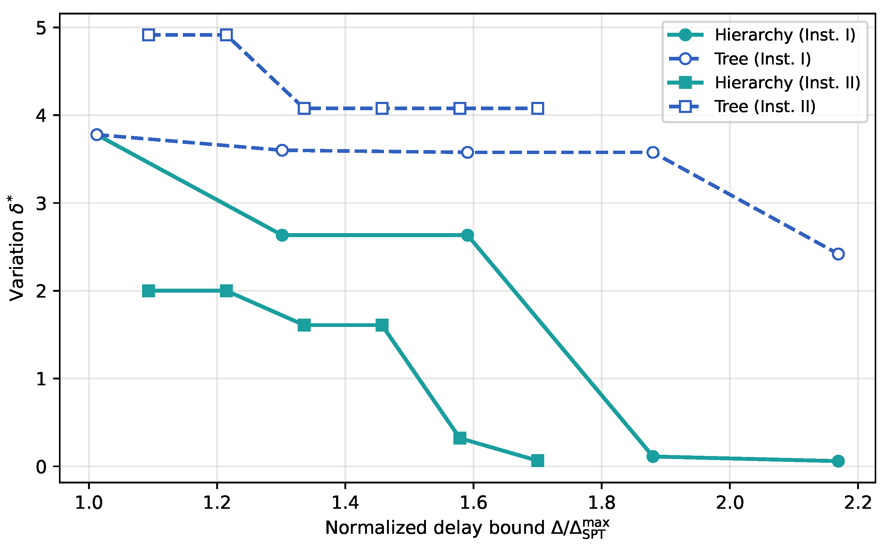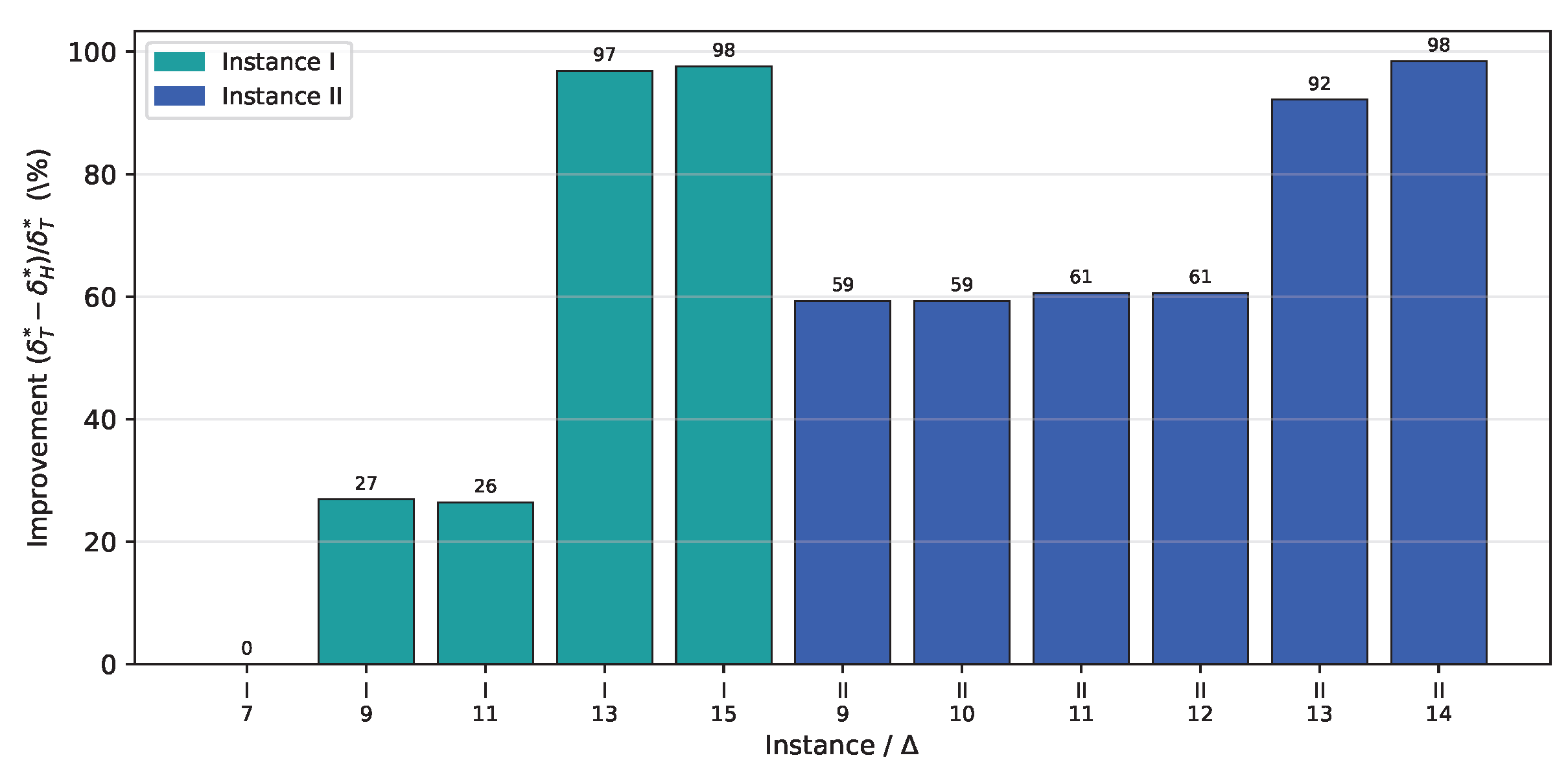Table 5 and Figure 9, Figure 10 and Figure 11 report results for both instances side by side.

Table 5. Hierarchy-based (ILP) versus tree-constrained (ILP) and CHAINS on Instances I and II (defined above), all values HiGHS proven-optimal. ${\delta }_H^{*}$ and ${\delta }_T^{*}$ denote the optimal hierarchy and tree variations; $J_H$ and $J_T$ are the corresponding Jain fairness indices. Dominance (${\delta }_H^{*}\le {\delta }_T^{*}$) holds in every row, consistent with Proposition 1.

Inst.	$\mathbf{\Delta }$	${\mathit{\delta }}_{\mathit{H}}^{*}$	Arcs Used	${\mathit{\delta }}_{\mathit{T}}^{*}$	Arcs Used	CHAINS $\mathit{\delta }$	$({\mathit{\delta }}_{\mathit{T}}^{*}-{\mathit{\delta }}_{\mathit{H}}^{*})/{\mathit{\delta }}_{\mathit{T}}^{*}$	${\mathit{J}}_{\mathit{H}}$	${\mathit{J}}_{\mathit{T}}$
I	7	3.7780	8	3.7780	8	3.7780	—	0.9462	0.9462
	9	2.6329	9	3.6007	10	2.6329	$27\%$	0.9819	0.9715
	11	2.6329	9	3.5767	10	2.6329	$26\%$	0.9819	0.9756
	13	0.1115	22	3.5767	10	3.3838	$97\%$	1.0000	0.9756
	15	0.0588	20	2.4183	11	3.3838	$98\%$	1.0000	0.9942
II	9	2.0005	16	4.9154	10	2.4168	$59\%$	0.9936	0.9380
	10	2.0005	16	4.9154	10	2.0005	$59\%$	0.9936	0.9380
	11	1.6091	19	4.0771	12	2.0005	$61\%$	0.9968	0.9782
	12	1.6091	19	4.0771	12	2.4846	$61\%$	0.9968	0.9782
	13	0.3206	24	4.0771	12	2.0005	$92\%$	0.9999	0.9782
	14	0.0641	27	4.0771	12	5.6250	$98\%$	1.0000	0.9782

Table 5. Hierarchy-based (ILP) versus tree-constrained (ILP) and CHAINS on Instances I and II (defined above), all values HiGHS proven-optimal. ${\delta }_H^{*}$ and ${\delta }_T^{*}$ denote the optimal hierarchy and tree variations; $J_H$ and $J_T$ are the corresponding Jain fairness indices. Dominance (${\delta }_H^{*}\le {\delta }_T^{*}$) holds in every row, consistent with Proposition 1.

Inst.	$\mathbf{\Delta }$	${\mathit{\delta }}_{\mathit{H}}^{*}$	Arcs Used	${\mathit{\delta }}_{\mathit{T}}^{*}$	Arcs Used	CHAINS $\mathit{\delta }$	$({\mathit{\delta }}_{\mathit{T}}^{*}-{\mathit{\delta }}_{\mathit{H}}^{*})/{\mathit{\delta }}_{\mathit{T}}^{*}$	${\mathit{J}}_{\mathit{H}}$	${\mathit{J}}_{\mathit{T}}$
I	7	3.7780	8	3.7780	8	3.7780	—	0.9462	0.9462
	9	2.6329	9	3.6007	10	2.6329	$27\%$	0.9819	0.9715
	11	2.6329	9	3.5767	10	2.6329	$26\%$	0.9819	0.9756
	13	0.1115	22	3.5767	10	3.3838	$97\%$	1.0000	0.9756
	15	0.0588	20	2.4183	11	3.3838	$98\%$	1.0000	0.9942
II	9	2.0005	16	4.9154	10	2.4168	$59\%$	0.9936	0.9380
	10	2.0005	16	4.9154	10	2.0005	$59\%$	0.9936	0.9380
	11	1.6091	19	4.0771	12	2.0005	$61\%$	0.9968	0.9782
	12	1.6091	19	4.0771	12	2.4846	$61\%$	0.9968	0.9782
	13	0.3206	24	4.0771	12	2.0005	$92\%$	0.9999	0.9782
	14	0.0641	27	4.0771	12	5.6250	$98\%$	1.0000	0.9782

Instances I and II are defined at the start of Section 5; Table 3 and Table 4 report Instance I. All reported values are computed with the HiGHS exact solver and are proven optimal; a lexicographic tie-break (minimize variation, then total delay) yields a unique delay vector, ensuring that the reported fairness indices are reproducible. The dominance inequality ${\delta }_H^{*}\le {\delta }_T^{*}$ holds in every row, as guaranteed by Proposition 1(i).

• Hierarchy versus tree (Figure 9).

Figure 9 plots the optimal delay variation ${\delta }^{*}$ as a function of $\Delta$ for both instances. All plotted values are proven-optimal. In Instance I the hierarchy achieves the same variation as the tree at the tightest feasible bound ($\Delta =7$, where the only feasible solution is the shortest-path tree), then pulls ahead: reductions of $27\%$ at $\Delta =9$, $26\%$ at $\Delta =11$, and $97\%$ at $\Delta =13$, reaching $98\%$ at $\Delta =15$ as the hierarchy attains near-perfect equalization (${\delta }_H^{*}=0.059$, $J_H=1.000$). In Instance II, where the SPT spread is larger ($5.82$ versus $3.78$), the tree is already considerably worse than the hierarchy at the first feasible bound: a $59\%$ reduction at $\Delta =9$ grows to $61\%$ at $\Delta =11$–12 and to $98\%$ at $\Delta =14$.

• Normalized comparison (Figure 10).

To facilitate comparison across instances with different delay scales, the delay bound is normalized by the maximum SPT delay ${\Delta }_{\mathrm{SPT}}^{max}$. Figure 10 plots the proven-optimal rows of both instances on a common axis. Three features are consistent: at $\Delta /{\Delta }_{\mathrm{SPT}}^{max}=1$ both instances coincide at the SPT spread; the hierarchy variation drops steeply as $\Delta$ increases while the tree variation declines slowly; and the hierarchy curves remain on or below the tree curves throughout, and strictly below once $\Delta$ exceeds the tightest feasible bound. This behavior is precisely what Proposition 1(iii) predicts: as $\Delta$ loosens, the hierarchy gains access to longer detour walks that further equalize destination delays, while the tree single-predecessor constraint prevents equivalent compensation.

• Improvement summary (Figure 11).

Figure 11 summarizes the percentage improvement $({\delta }_T^{*}-{\delta }_H^{*})/{\delta }_T^{*}$ for every (proven-optimal) row across both instances. Improvements range from $26\%$ at the tightest non-trivial bounds to $98\%$ where the hierarchy attains near-perfect equalization. Because all values are proven-optimal, each percentage is a certified gap rather than a bound. No row in either instance violates dominance, confirming Proposition 1(i) empirically across both topologies.

• Heuristic comparison.

CHAINS, the most robust heuristic in the DVBMT lineage, achieves the same variation as the ILP hierarchy in Instance I at $\Delta =9$ and $\Delta =11$, but diverges significantly for $\Delta \ge 13$. In Instance II, CHAINS matches the hierarchy only at $\Delta =10$ and reverts to near-SPT performance for $\Delta \ge 13$, even returning a variation ($5.625$) above the tree optimum ($4.077$) at the loosest bound. DVMA and FCHAINS coincide with the SPT solution across all tested bounds in both instances; they are reported for completeness, since both heuristics were designed for the regime in which an explicit variation constraint is active, not the free-variation setting used here. This pattern reflects the absence of any optimality guarantee: as a greedy, shortest-path-anchored method, CHAINS locates the delay-equalizing reconvergence only intermittently and need not be monotone in $\Delta$, which motivates the exact treatment pursued here. Because every reported ILP value is proven-optimal, the improvement over CHAINS is a certified gap rather than a lower bound, and the exact formulation certifies the equalizing hierarchy whenever one exists.

• Summary.

Two independently generated instances, different sizes ($n\in \{12,15\}$), different group sizes ($\left|M\right|\in \{7,8\}$), and different SPT spreads all yield the same qualitative finding: ILP-optimal hierarchies consistently and substantially outperform both tree-constrained ILP solutions and the published heuristics, including CHAINS, the strongest of them. The absolute improvement is largest at intermediate delay bounds, where feasible alternatives exist, but the SPT spread remains large; the relative improvement grows as $\Delta$ is relaxed. Hierarchy dominance is present throughout, and is largest in the regime of large SPT spread, where fairness is most critical. Crucially, the dominance also holds under an independent fairness measure: in every row of Table 3, Table 4 and Table 5 the hierarchy’s Jain index meets or exceeds the tree’s, rising toward 1 as $\Delta$ is relaxed. Jain’s index is not optimized by the ILP (it is non-linear, cf. Section 2.4); it is reported post hoc as a member of the Lan et al. [16] family, so its agreement with the ${\delta }^{*}$ ranking confirms that the hierarchy advantage is a property of the solutions, not an artifact of the particular operational objective the ILP minimizes.

5.2. Sensitivity Analysis of Heuristic Performance

The preceding case study evaluates two fixed instances. To assess the generalizability of the observed heuristic behavior across the problem parameter space, a controlled sensitivity analysis is conducted over six independent dimensions: the delay bound $\Delta$, network size n, graph density p, multicast group size $\left|M\right|$, arc delay heterogeneity, and the CHAINS candidate-path parameter k. Each experiment varies one parameter while holding all others at a baseline configuration ($n=12$, $\left|M\right|=7$, $p=0.35$, delays in $[2,5]$, costs in $[1,10]$, $\Delta =1.5\times {max}_{m\in M}{d}_{\mathrm{SPT}}(s,m)$, $k=5$). For every parameter value, 40 independent Erdős–Rényi instances are generated; instances in which the SPT delay span is below $1.5$ time units are discarded and replaced. All reported values are means over the 40 qualifying instances. DVMA and FCHAINS are omitted from the figures below because, under unconstrained variation (${\delta }_{\mathrm{var}}=\infty$), both produce routing trees identical to SPT in every sampled instance, confirming that they only diverge from SPT when an explicit variation bound is active.

We select CHAINS [14] as the sole polynomial-time benchmark for three reasons documented in the DVBMT literature.

(i)

Solution quality: CHAINS was introduced explicitly to escape the SPT baseline via a k-shortest-path exploration. In the free-variation setting used here, it matches the hierarchy ILP optimum whenever a tree can attain it (Table 5: Instance I at $\Delta =9,11$; Instance II at $\Delta =10$), whereas DVMA and FCHAINS coincide with SPT across every tested bound in both instances. They are therefore reported for completeness in the case-study tables but omitted from the sensitivity figures.

(ii)

Complexity comparability: Alternatives that couple metaheuristic search with a variation-constrained objective—SADDVMA (simulated annealing, [35]), the tabu-search construction in [36], and the ant-based method in [33]—target the constrained-Steiner variant (cost objective, $\delta$ as constraint) rather than the free-variation minimization studied here. Their published results are not directly comparable to our $\delta$-minimization setting.

(iii)

Absence of an optimality certificate: The essential contrast the paper wishes to draw is between the strongest published DVBMT heuristic and the certified ILP optimum. Adding further heuristics that lack an optimality certificate would broaden, but not sharpen, this contrast.

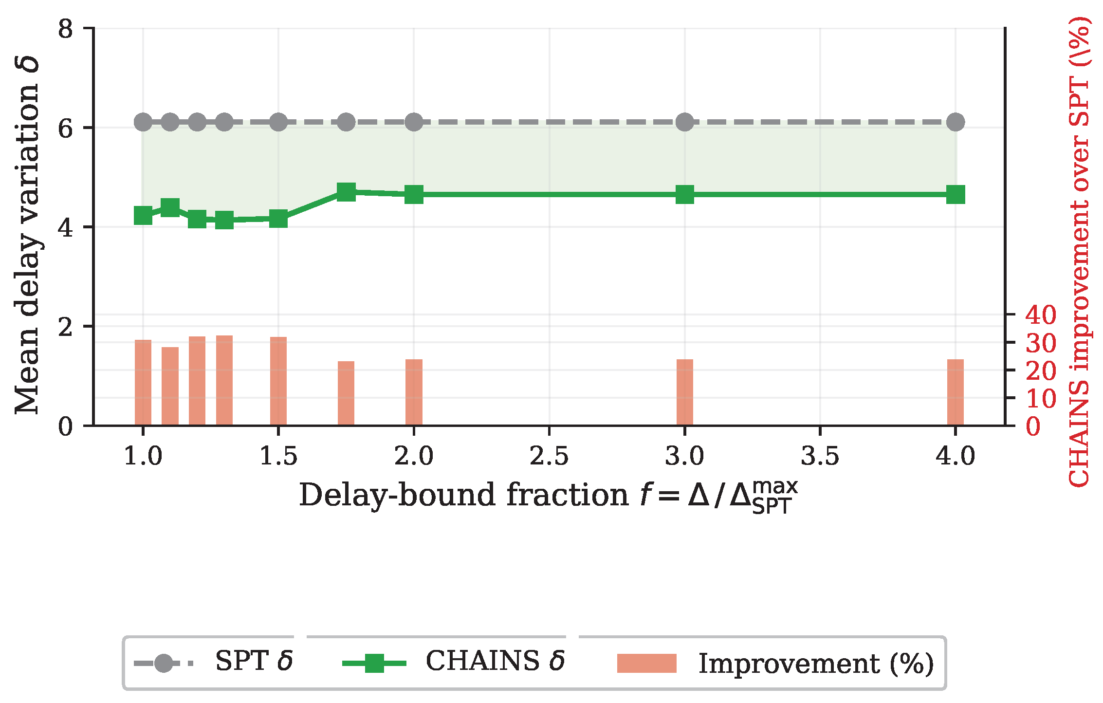
5.2.1. Sensitivity to Delay Bound (SA-1)

The delay bound is expressed as a fraction $f=\Delta /{\Delta }_{\mathrm{SPT}}^{max}$ and swept from $f=1.0$ to $f=4.0$. Figure 12 shows the mean delay variation for SPT and CHAINS (left axis, lines) together with the percentage improvement of CHAINS over SPT (right axis, bars). CHAINS achieves its maximum improvement of $32.3\%$ at $f=1.3$, where the bound is tight enough to force path diversification, but loose enough for k-path alternatives to exist. Improvement stabilizes at approximately $24\%$ for $f\ge 2.0$, indicating diminishing returns from additional delay budget. Because CHAINS is itself a heuristic, the true ILP-hierarchy optimum would yield even greater improvement in the tight-$\Delta$ regime ($f\in [1.0,1.5]$), where Proposition 1 provides the most additional flexibility.

5.2.2. Sensitivity to Network Size (SA-2)

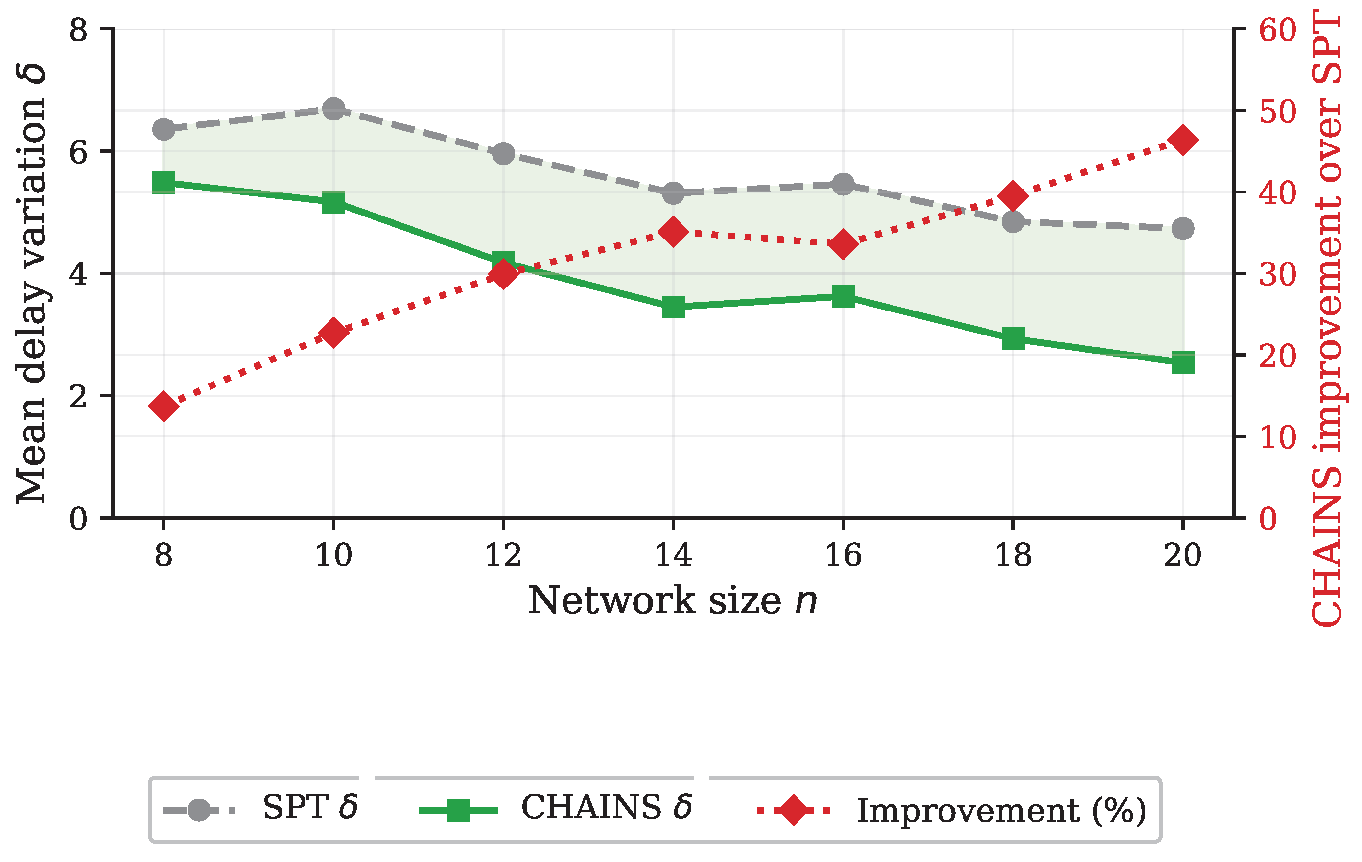
Network size is swept from $n=8$ to $n=20$. Figure 13 plots mean variation (left axis) and CHAINS improvement rate (right axis). Both SPT and CHAINS variation decrease monotonically with n because larger networks offer exponentially more candidate paths. Crucially, the improvement rate rises from $24.6\%$ at $n=8$ to $34.6\%$ at $n=20$ (peaking near $38\%$ at $n=18$), with a mean variation gap on the order of $1.6$–$1.9$ time units. The CHAINS-over-SPT improvement rate therefore rises with n. Whether the exact tree–hierarchy gap behaves the same way is a separate question that this heuristic sweep does not answer; it is measured directly in Section 5.3, where the relative gap is found to be large but not increasing in n over the tested range.

5.2.3. Sensitivity to Graph Density and Group Size (SA-3, SA-4)

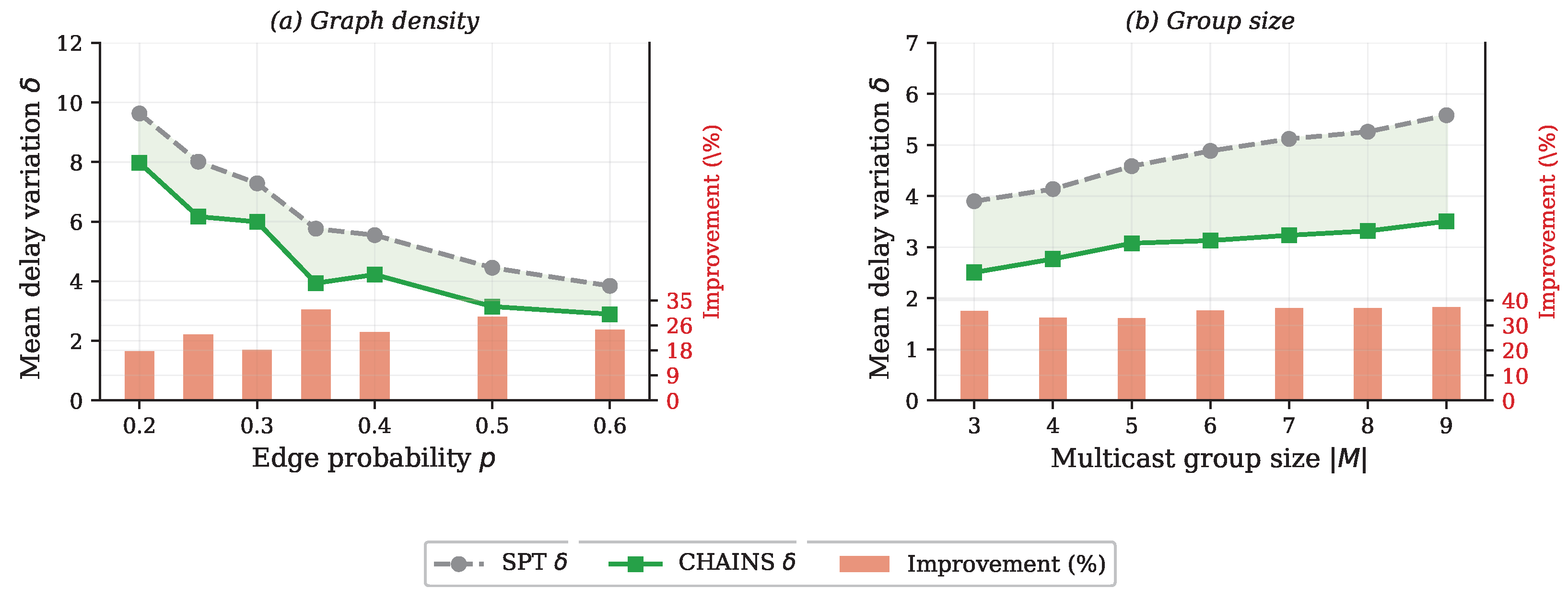
Figure 14 presents two structural parameters side by side. Panel (a) sweeps graph density from $p=0.20$ (sparse) to $p=0.60$ (dense). Graph density is among the most influential parameters on absolute variation levels: SPT variation drops from $9.67$ at $p=0.20$ to $3.81$ at $p=0.60$, a $61\%$ reduction driven by topological richness. The steep decline between $p=0.20$ and $p=0.35$ indicates that a minimum connectivity threshold is required for meaningful fairness optimization. Real-world backbone networks typically have densities in the $0.10$–$0.30$ range [38], placing them in the regime where hierarchy-based formulations are most beneficial.

Panel (b) sweeps the multicast group size from $\left|M\right|=3$ to $\left|M\right|=9$ on a fixed $n=14$ topology. SPT variation increases from $3.54$ to $5.87$ ($+66\%$) because more destinations increase the number of pairwise delay differences to control for. CHAINS maintains a stable improvement ratio of 28–$36\%$ across all group sizes, and the cost overhead over SPT rises proportionally with $\left|M\right|$, quantifying the price of fairness as a near-linear function of group size.

5.2.4. Sensitivity to Arc Delay Heterogeneity (SA-5)

Arc delay heterogeneity is the most influential parameter, producing the widest range of variation across its sweep. Mean SPT variation scales roughly linearly with the delay range width: from $4.29$ at $[2,3]$ (width 1) to $13.85$ at $[1,15]$ (width 14), a $3.2\times$ increase. CHAINS improvement remains stable between $25\%$ and $35\%$ across all ranges, demonstrating robustness to the shape of the delay distribution. Networks with heterogeneous link technologies (e.g., mixed wired and wireless segments) represent the primary application domain in which fairness-aware routing yields the greatest absolute benefit.

5.2.5. CHAINS k-Path Parameter (SA-6)

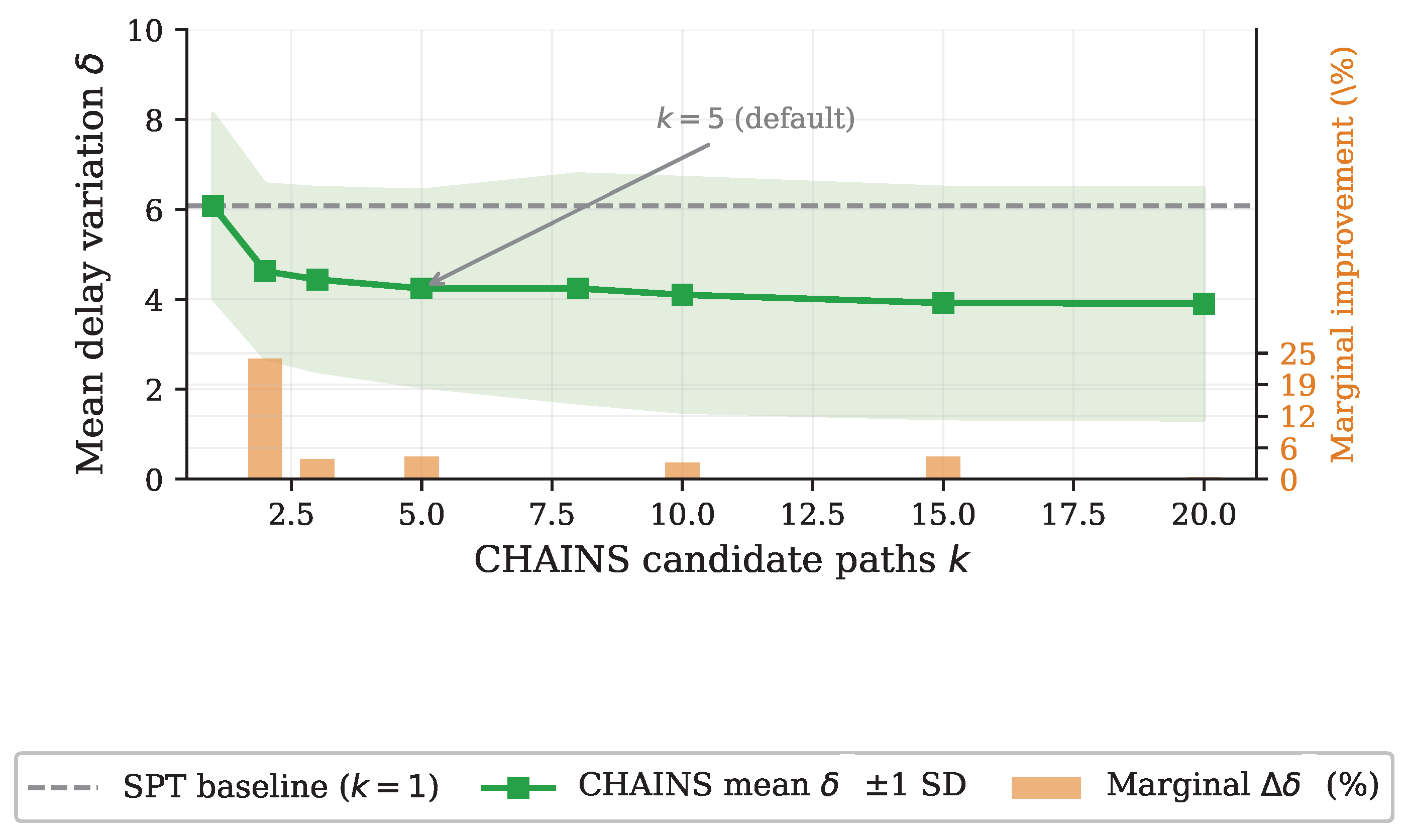
Figure 15 shows mean variation with $\pm 1$ standard deviation (left axis, shaded band) and marginal improvement per unit increase in k (right axis, bars). The single largest marginal improvement occurs at $k=2$ ($17.0\%$ reduction versus $k=1$). From $k=2$ to $k=7$ the mean improvement rises gradually to a peak of $25.3\%$ at $k=7$; beyond $k=7$ no further benefit is observed, and mean variation is essentially flat (indeed marginally higher for very large k). Since increasing k past 5 yields well under one additional time unit of improvement while runtime grows substantially, the default $k=5$ remains a sound trade-off between solution quality and computational effort.

5.2.6. Parameter Ranking and Consolidated Findings

Table 6. Parameter sensitivity ranking by influence on ${\delta }^{*}$ (SPT-variation range across each sweep; 40 instances/point, seed base 1000).

Rank	Parameter	Level	${\mathit{\delta }}^{*}$ Range	Key Observation
1	Delay range	High	4.29–13.85	${\delta }^{*}$ scales near-linearly with range width ($4.29\to 13.85$, $3.2\times$)
2	Graph density p	High	3.81–9.67	SPT ${\delta }^{*}$ drops $61\%$ ($9.67\to 3.81$), steepest for $p=0.20\to 0.35$
3	Network size n	Medium	4.54–7.02	CHAINS improvement rises $24.6\%$ ($n=8$) → $34.6\%$ ($n=20$)
4	Group size $\left|M\right|$	Medium	3.54–5.87	SPT ${\delta }^{*}$ up $66\%$ ($\left|M\right|=3\to 9$); cost overhead near-linear in $\left|M\right|$
5	CHAINS k	Low	4.56–6.11	Marginal gain plateaus beyond $k=$ 5–7
6	$\Delta$ bound	Low	4.14–4.65	SPT is $\Delta$-invariant; CHAINS shifts by $\le 0.5$ units across the sweep

ranks the six parameters by their influence on absolute variation levels. Three findings directly support the manuscript’s theoretical contributions:

(i) 

The two highest-impact parameters, arc delay range width and graph density, are the structural features identified after Remark 1 as driving a substantive tree-hierarchy gap. Variation scales near-linearly with delay heterogeneity (SA-5) and falls by $61\%$ as density rises (SA-3). This confirms that the sparse, delay-heterogeneous regime is where fairness is hardest for tree-restricted methods.

(ii) 

The CHAINS-over-SPT improvement (24–$37\%$) is robust across all six sweeps but plateaus in the k-path budget beyond $k=5$–7 (SA-6). Additional tree-restricted search effort cannot pass the structural floor ${\delta }_T^{*}$ established by Proposition 1 and its Corollary 1.

(iii) 

SPT variation is invariant in the delay bound $\Delta$ (SA-1), showing that the variation floor is governed by topology and delay heterogeneity rather than the delay budget—the same pinning mechanism that Proposition 1(iii) isolates and the Abilene study exhibits.

In summary, the qualitative ordering among heuristics is preserved across all six dimensions, and the CHAINS improvement over SPT (24–$37\%$) is robust across delay heterogeneity and group size. The parameters with the highest practical impact—arc delay heterogeneity and graph density—identify the application regime where the exact ILP hierarchy methods provide the most value: sparse networks with heterogeneous link delays, precisely the conditions typical of real-world backbone topologies [38].

5.3. Distribution of the Exact Tree–Hierarchy Gap

The sensitivity study above varies only the heuristics (SPT, CHAINS); it does not solve the exact tree and hierarchy ILPs, and therefore characterizes heuristic behavior rather than the quantity of primary interest, the proven-optimal relative gap $({\delta }_T^{*}-{\delta }_H^{*})/{\delta }_T^{*}$. To report that gap as a distribution rather than on the three fixed topologies of Section 5.1, Section 5.2, Section 5.3 and Section 5.4, we solve both the hierarchy and the tree min-variation ILPs to proven optimality with HiGHS on 40 independent Erdős–Rényi instances at each of three sizes ($n\in \{10,12,14\}$, $\left|M\right|=5$, $p=0.35$, arc delays in $[2,5]$, $\Delta =1.5\times {max}_{m\in M}{d}_{\mathrm{SPT}}(s,m)$). Since $\Delta \ge {max}_m{d}_{\mathrm{SPT}}(s,m)$, the shortest-path tree is always delay-feasible, so ${\delta }_T^{*}$ is finite on every instance, and the ratio is well defined.

Table 7. Distribution of the proven-optimal relative gap $({\delta }_T^{*}-{\delta }_H^{*})/{\delta }_T^{*}$ over 40 random Erdős–Rényi instances per size ($\left|M\right|=5$, $p=0.35$, $\Delta =1.5\times$ max SPT delay; HiGHS proven-optimal). “>0” is the fraction of instances with a strictly positive gap; $\overline{{\delta }_H^{*}}$ and $\overline{{\delta }_T^{*}}$ are the mean optimal hierarchy and tree variations.

n	Median	IQR	Mean	>0	$\overline{{\mathit{\delta }}_{\mathit{H}}^{*}}$	$\overline{{\mathit{\delta }}_{\mathit{T}}^{*}}$
10	$92.0\%$	$[75.8,96.4]\%$	$83.4\%$	$97.5\%$	$0.52$	$3.71$
12	$88.0\%$	$[80.8,94.4]\%$	$78.1\%$	$95.0\%$	$0.43$	$2.11$
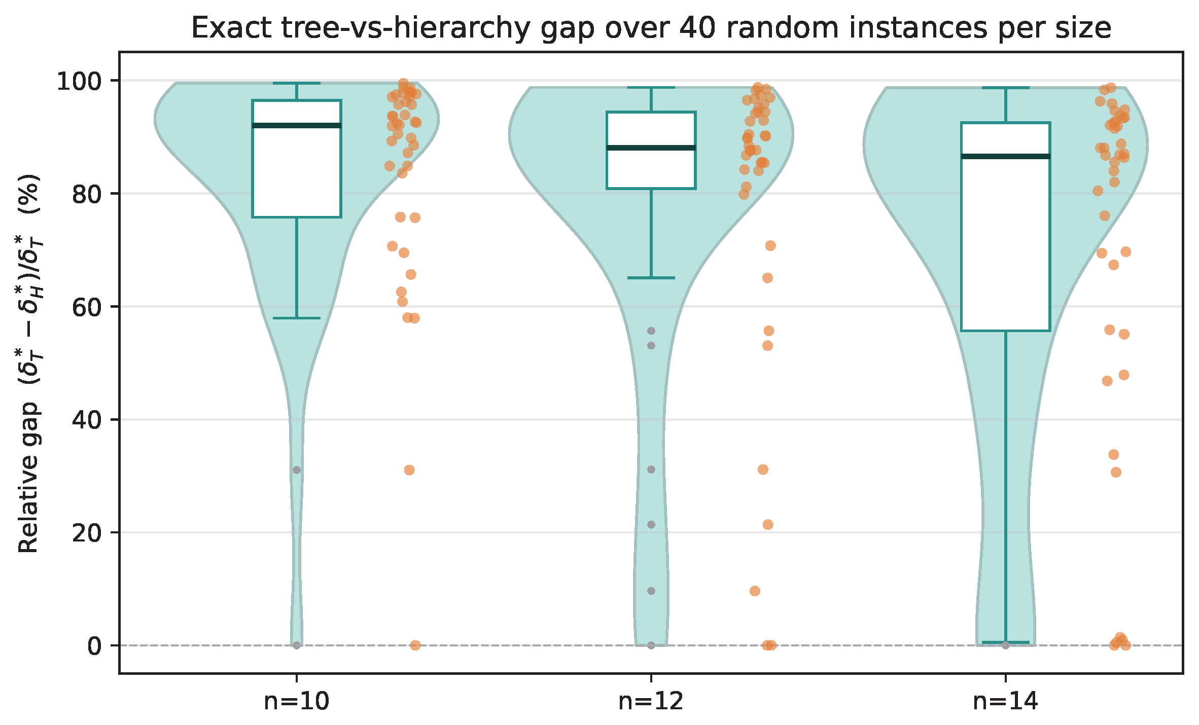
14	$86.5\%$	$[55.7,92.5]\%$	$70.5\%$	$95.0\%$	$0.36$	$1.14$

and Figure 16 summarize the 120 instances.

Two conclusions follow, both resting on proven-optimal values rather than heuristic estimates. First, the hierarchy gap is not an artifact of the three hand-picked topologies: across 120 random instances the tree-to-hierarchy reduction has a median of 86–$92\%$ and is strictly positive on 95–$98\%$ of instances. The few near-zero cases are exactly the conditional ties anticipated by the scope Remark following Proposition 1—instances on which a tree happens to reproduce the hierarchy’s equalization—so their presence confirms, rather than weakens, the conditional reading of part (iii). Second, over the tested range the relative gap does not grow with n; it declines slightly (mean $83.4\%$ at $n=10$ to $70.5\%$ at $n=14$). This is because denser instances at larger n offer more near-equal shortest-path alternatives and a smaller absolute tree spread ($\overline{{\delta }_T^{*}}$ falls from $3.71$ to $1.14$). Operationally, this highlights the benefit of the exact method. The advantage is largest on sparse, high-spread topologies, the regime where shortest-path delays diverge most and fairness is hardest to achieve. It is smaller on dense graphs, where near-equal alternative paths allow even a tree to approach equalization. The density sweep of Figure 14 makes this trend explicit, with the gap narrowing monotonically as the edge probability p rises.

5.4. Real-Topology Evaluation on the Abilene Backbone

To quantify the magnitude of the hierarchy gain on a standard real topology, rather than on synthetic Erdős–Rényi instances, we evaluate the exact formulations on the Abilene (Internet2) backbone, a standard real topology with 11 nodes and 14 bidirectional links (28 directed arcs). One-way arc delays are set to fiber propagation derived from inter-city great-circle distance ($5\mathsf{\mu }\mathrm{s}/\mathrm{km}$), and arc costs are taken proportional to distance. 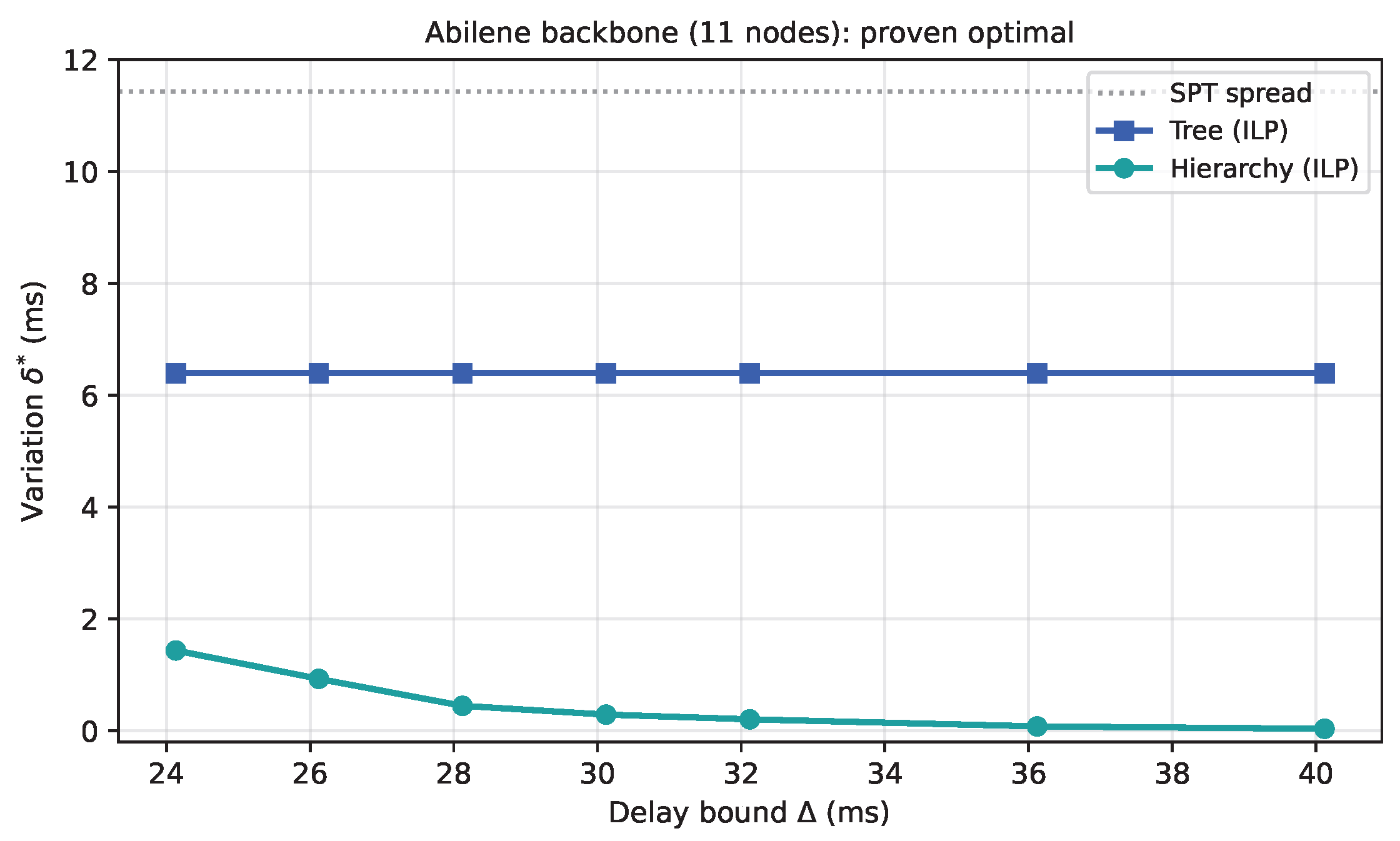The source is Seattle and the multicast group is $M=$ {Houston, Atlanta, New York, Washington, Chicago, Kansas City}, giving a maximum SPT delay of $24.12$ ms and an SPT spread of $11.43$ ms. Both the hierarchy and the tree variant are solved to proven optimality with HiGHS over a sweep of $\Delta$ (Table 8, Figure 17).

Table 8. Abilene backbone (11 nodes), proven-optimal hierarchy vs. tree. ${\delta }^{*}$ and Jain index of the optimal delay vector at each delay bound $\Delta$ (ms). The tree optimum is pinned well above zero (and below the raw SPT spread of $11.43$ ms); the hierarchy drives variation toward zero.

$\mathbf{\Delta }$ (ms)	${\mathit{\delta }}_{\mathit{H}}^{*}$	${\mathit{J}}_{\mathit{H}}$	${\mathit{\delta }}_{\mathit{T}}^{*}$	${\mathit{J}}_{\mathit{T}}$	Reduction
24.13	1.434	0.9995	6.393	0.9850	78%
26.12	0.927	0.9998	6.393	0.9850	86%
28.12	0.444	1.0000	6.393	0.9850	93%
30.12	0.288	1.0000	6.393	0.9850	96%
32.12	0.203	1.0000	6.393	0.9850	97%
36.12	0.077	1.0000	6.393	0.9850	99%
40.12	0.034	1.0000	6.393	0.9850	99%

Table 8. Abilene backbone (11 nodes), proven-optimal hierarchy vs. tree. ${\delta }^{*}$ and Jain index of the optimal delay vector at each delay bound $\Delta$ (ms). The tree optimum is pinned well above zero (and below the raw SPT spread of $11.43$ ms); the hierarchy drives variation toward zero.

$\mathbf{\Delta }$ (ms)	${\mathit{\delta }}_{\mathit{H}}^{*}$	${\mathit{J}}_{\mathit{H}}$	${\mathit{\delta }}_{\mathit{T}}^{*}$	${\mathit{J}}_{\mathit{T}}$	Reduction
24.13	1.434	0.9995	6.393	0.9850	78%
26.12	0.927	0.9998	6.393	0.9850	86%
28.12	0.444	1.0000	6.393	0.9850	93%
30.12	0.288	1.0000	6.393	0.9850	96%
32.12	0.203	1.0000	6.393	0.9850	97%
36.12	0.077	1.0000	6.393	0.9850	99%
40.12	0.034	1.0000	6.393	0.9850	99%

The result is sharper than on the synthetic instances. The tree optimum is pinned at ${\delta }_T^{*}=6.393$ ms (Jain $0.985$) for every value of $\Delta$: the single-predecessor restriction prevents the tree from lengthening any path to equalize delays, so relaxing $\Delta$ buys it nothing. The hierarchy, by contrast, exploits the additional delay budget to reduce ${\delta }_H^{*}$ from $1.434$ ms down to $0.034$ ms (Jain $\to 1$), a $78\%$ reduction already at the tightest feasible bound and $99\%$ once $\Delta$ is relaxed. Unlike the synthetic case study, where tree and hierarchy coincide at the tightest bound, on Abilene the hierarchy strictly dominates the tree at every tested bound on this topology, confirming that the structural advantage established in Proposition 1 is realized on operational backbone topologies.

Robustness of the Abilene reading: Four choices determine the Abilene numbers reported above: the link-delay assignment, the source, the destination set, and the $\Delta$ range. We comment on each.

(i) 

The $5\mathsf{\mu }\mathrm{s}/\mathrm{km}$ propagation-delay proxy is the standard inter-city-distance conversion used in the Topology Zoo [38] and matches the fiber propagation constant (∼5 µs/km); scaling all arc delays by a common factor rescales ${\delta }^{*}$, $\Delta$, and the pinning value ${\delta }_T^{*}=6.393$ ms proportionally, so relative reductions (the 78–$99\%$ column of Table 8) are unaffected. Adding queuing components on top of propagation would loosen ${\delta }_H^{*}$ but keep the tree pinning intact, because the single-predecessor obstruction is topological rather than metric.

(ii) 

Seattle is deliberately chosen as a coast-to-coast diameter endpoint that maximizes the SPT spread ($11.43$ ms). Repeating the experiment with Sunnyvale or Denver as the source shrinks the SPT spread and, hence, the absolute ${\delta }_T^{*}$, but the tree’s structural pinning behavior persists as long as the destination set spans both coasts.

(iii) 

The destination set covers six of the ten non-source Abilene POPs and spans the north-east/south diameter; removing individual destinations reduces the number of active Proposition 1(ii) bottlenecks and can lower ${\delta }_T^{*}$, but the qualitative ${\delta }_H^{*}\ll {\delta }_T^{*}$ ordering is stable across such perturbations because it is guaranteed by Proposition 1(i).

(iv) 

$\Delta$ is swept from the tightest feasible bound ($24.13$ ms, the maximum SPT delay) upward, so no result depends on a preferential single-$\Delta$ choice. Consequently, the reported hierarchy gain on Abilene is a robust operational finding rather than an artifact of the specific link-delay assignment or a particular source–destination fit.

5.5. Exact ILP Scalability

The sensitivity study of Section 5.2 varies network size only for the heuristics. To characterize the exact method itself, we solve the hierarchy min-variation ILP to proven optimality on random instances of growing size ($\left|M\right|=5$, $\Delta =1.5\times$ max SPT delay, HiGHS with a per-solve time cap).

Table 9. Exact hierarchy ILP scalability. Binary-variable count is $\left|A\right|\left(\right|M|+1)$ (the pairwise sharing family dominates). Three random seeds per size up to $n=14$ and two for $n\ge 16$, where per-instance certification runtime makes further replicates costly; the $n\ge 16$ timing statistics are therefore indicative rather than a characterized distribution, whereas the optimality of every reported instance is proven regardless of the seed count. Every instance up to $n=20$ is solved to proven optimality.

n	$\left|\mathit{A}\right|$	Binaries	Proven	Mean (s)	Max (s)
8	19	114	3/3	0.1	0.1
10	31	186	3/3	0.1	0.2
12	41	246	3/3	13.6	28.1
14	56	336	3/3	0.6	1.7
16	70	420	2/2	37.5	73.0
18	91	546	2/2	43.4	77.4
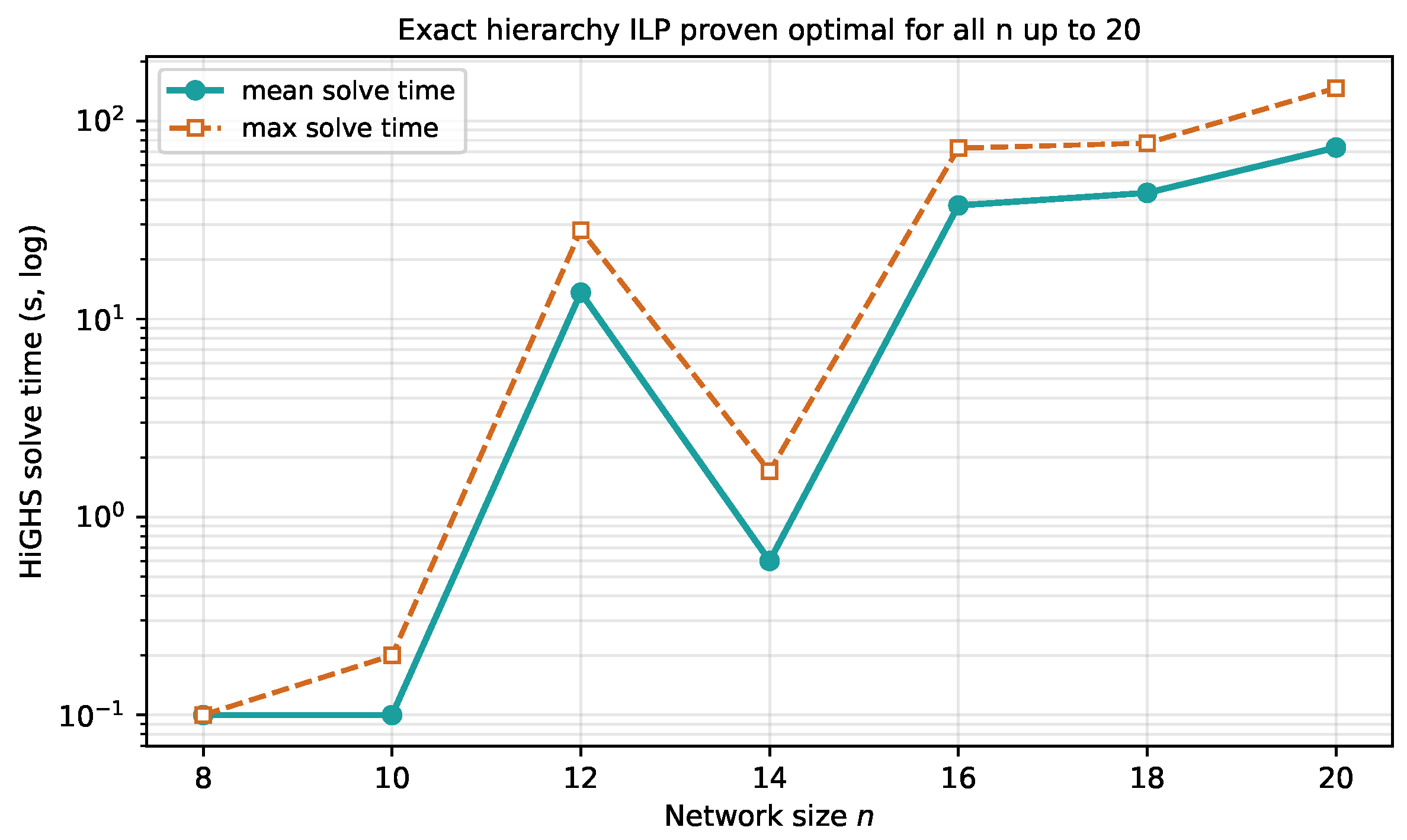
20	107	642	2/2	73.5	146.8

and Figure 18 report the problem size and solve time as a function of n. This establishes the regime over which the exact method delivers proven-optimal fairness solutions. Two pieces of evidence combine to define that regime.

(i) 

Proven optimality at operational sizes: Every instance up to $n=20$, spanning the 8–20 range used across the heuristic sensitivity study, is closed with an optimality certificate; the real-topology Abilene study of Section 5.4 solves an 11-node, 28-arc backbone with $\left|M\right|=6$ to proven optimality across seven values of $\Delta$.

(ii) 

Coverage across random instances: The gap-distribution study of Section 5.3 certifies optimality on 120 additional random instances at $\left|M\right|=5$, complementing the fixed-topology case studies. Beyond the tested envelope—dense meshes, larger groups ($\left|M\right|>5$), or carrier-grade backbones ($n>20$)—the pairwise-sharing block dominates and the exact solve becomes costly; the natural target is the Benders/branch-and-price direction listed in future work, exploiting the per-destination-pair structure of $\sigma (m,n,a)$ (Equations (24)–(27)).

Two observations follow. First, proven optimality is attainable across the whole $n=8$–20 range studied for the heuristics, so the exact method is a viable ground truth on instances of the size used in our case studies (with two to three seeds per size, the $n\ge 16$ timings are indicative rather than a characterized distribution; the scalability claim is that proven optimality is attainable across $n=8$–20, not that the runtime distribution at $n\ge 16$ is fully characterized), not merely on the two case-study topologies. Second, solve time is non-monotonic in n (e.g., $n=12$ is harder than $n=14$): the binding factor is the optimal variation itself—instances whose optimum approaches zero require the solver to certify a near-perfectly equalized delay vector, which is combinatorially the hardest regime—rather than raw size. The binary count grows as $\left|A\right|\left(\right|M|+1)$, dominated by the per-destination sharing variables, which identifies the pairwise-sharing block as the natural target for the Benders or branch-and-price decomposition noted below.

6. Conclusions

This paper studies fairness-aware multicast routing under the two operational parameters that structure the equitable-optimization literature: the maximum end-to-end delay $\Delta$ (a Rawlsian worst-case cap) and the inter-destination delay variation $\delta$ (a bounded-inequality no-envy-within-threshold criterion). The core contribution is structural: the feasible region of the underlying optimization problem is the family of partial spanning hierarchies, and partial spanning trees are strictly the special case obtained by imposing a single-predecessor constraint on every node. Proposition 1 makes this precise. Part (i) gives the containment ${\mathcal{F}}_T\subseteq {\mathcal{F}}_H$ and the induced inequality ${\delta }_H^{*}\le {\delta }_T^{*}$, both by construction. Part (ii) exhibits a bottleneck-and-hub instance family on which the containment is strict. Part (iii), together with Remark 1, provides a sufficient condition—a reconvergence node at which the hierarchy’s differing upstream delays offset the fixed downstream imbalance—under which the gap is quantified as ${\delta }_T^{*}-{\delta }_H^{*}\ge \epsilon >0$. The Corollary 1 that follows converts the same statement into a certified performance ceiling for every tree-restricted heuristic.

On the algorithmic side, we present a family of flow-based ILP formulations (Section 4) that share one constraint skeleton across four objectives (cost, per-destination delay, maximum delay, and maximum pairwise variation) and toggle between the hierarchy and tree feasible regions through the single-predecessor constraint (17). This makes the tree-versus-hierarchy comparison a controlled experiment within one model rather than a comparison across unrelated formulations, and it makes every reported gap between the two a certified quantity rather than a heuristic estimate.

The experimental study (Section 5) reports what the enlargement of the feasible region buys empirically. On two independent Erdős–Rényi instances (Section 5.1), the hierarchy optimum matches the tree at the tightest feasible bound and pulls ahead thereafter, reaching a 97–$98\%$ reduction as $\Delta$ is relaxed. A six-parameter sensitivity study (Section 5.2) identifies arc delay heterogeneity and graph density—exactly the structural features Remark 1 anticipates—as the two highest-impact drivers of the variation floor. A 120-instance gap-distribution study (Section 5.3) reports a median proven-optimal reduction of 86–$92\%$ and a strictly positive gap on 95–$98\%$ of instances, with the residual near-zero tail matching the conditional-tie regime Remark 1 delimits. On the Abilene backbone (Section 5.4), the tree optimum is pinned at ${\delta }_T^{*}=6.393$ ms across every value of $\Delta$—the pinning mechanism of Proposition 1(iii) exhibited on a real topology—while the hierarchy reduces the variation by $78\%$ at the tightest feasible bound and by $99\%$ once $\Delta$ is relaxed. Every reported optimum is certified by the HiGHS solver, and the scalability sweep of Section 5.5 closes with optimality certificates up to $n=20$.

Together, the structural and empirical results place the paper’s central claim inside a clear scope. The dominance ${\delta }_H^{*}\le {\delta }_T^{*}$ holds by construction. Whether the gap is cosmetic or substantial is an empirical question, and the answer identifies the sparse, delay-heterogeneous regime characteristic of real backbones as the operating point at which the exact hierarchy formulation is most valuable and tree-restricted heuristics are structurally furthest from the certified optimum.

6.1. Limitations

Five limitations bound the scope of these results. First, while the inequality ${\delta }_H^{*}\le {\delta }_T^{*}$ is guaranteed by Proposition 1(i) for every instance, the gap magnitude is reported only for $\left|M\right|=5$ and $n\le 14$. It is characterized as a distribution over 120 random instances (Section 5.3). Its behavior for larger groups and networks, where exact solutions become costly, remains to be mapped. Second, the strict-separation guarantee of parts (ii)–(iii) depends on the bottleneck reconvergence structure. Without that obstruction, trees may match hierarchies for specific bounds, as the near-zero tail of Figure 16 shows empirically. Third, the pairwise sharing block introduces $O\left(\right|A\left|\right|M{|}^2)$ variables. Along with the difficulty of certifying near-zero variation, this limits the exact solution to roughly $n\le 20$ in our experiments (the $n\ge 16$ timing statistics are indicative rather than a characterized distribution, per the reduced seed count of Table 9). Larger instances require the decomposition methods outlined below.

Fourth, the operational cost of hierarchies. The mathematical dominance ${\delta }_H^{*}\le {\delta }_T^{*}$ does not imply that a hierarchy is always the preferred operational choice. Hierarchies replace the single-predecessor tree property with a more general reconvergence structure in which some nodes carry per-destination forwarding state across multiple upstream branches. Thus, the per-node forwarding table size grows with $\left|M\right|$ rather than with the tree degree. The resulting delivery structure is more complex to deploy within protocols standardized for tree-shaped multicast (Protocol Independent Multicast–Sparse Mode (PIM-SM) and Multicast Listener Discovery (MLD)). In deployment contexts where implementation simplicity, per-node forwarding overhead, or compatibility with tree-only multicast protocols dominate the delay-fairness objective, or where the SPT spread is already small so the hierarchy gain would be marginal (cf. Remark 1 and Section 5.3), a tree solution can be preferable despite a strictly larger ${\delta }_T^{*}$. The paper’s contribution in such contexts is that the multi-constrained Steiner tree row in Table 2 still supplies a certified optimum, so the delay-fairness cost of the tree restriction is quantified rather than assumed.

Fifth, the delay-variation–cost trade-off. With $\Delta$ as a hard constraint and $\delta$ (equivalently $z_{\mathrm{var}}$) as the objective, tightening $\delta$ typically pushes routes onto longer alternative walks with higher OF1 cost. On Instance I, driving ${\delta }^{*}$ from $2.63$ (at $\Delta =11$) to $0.11$ (at $\Delta =13$) raises the ILP hierarchy cost from 57 to 140 and the arc count from 9 to 22 (Table 3), a $2.5\times$ cost of fairness. This is the classical price-of-fairness trade-off [13,18] in our formulation. That is why we recommend the first multi-objective row in Table 2, which combines OF1 with the variation objective (OF4). This can be either a Pareto front computed by the augmented $\epsilon$-constraint method [39] or a weighted scalarization where the operator picks the point on the $\delta$–cost frontier reflecting operational priorities. Excessive detours, meaning large cost increases for small $\delta$ gains, are exactly the frontier points a decision-maker would discard. The exact formulation makes them identifiable rather than hiding them inside a heuristic.

6.2. Future Work

Future research directions extend the present study along four axes. First, larger real-world topologies and decomposition: Section 5.4 establishes proven-optimal results on the Abilene backbone, and Section 5.5 certifies optimality up to $n=20$. Scaling to larger Topology Zoo/SNDlib instances such as AT&T North America (25 nodes) and GÉANT (22 nodes) will require the decomposition methods noted below, since the pairwise-sharing block grows as ${\left|A\right|\left|M\right|}^2$. Second, buffering and controlled latency: Extending the ILP to incorporate queuing-latency decision variables would enable modeling of controlled buffering at intermediate nodes. This allows analysis of the interaction between buffering policies and optimal routing (as discussed in [13]). Third, valid inequalities and Benders decomposition: Deriving valid inequalities or Benders cuts that exploit the hierarchical feasible region structure (Proposition 1) is expected to reduce the integrality gap and improve ILP scalability for larger instances. Fourth, analytical optimality-gap bounds: Establishing analytical lower bounds on the optimality gap of tree-restricted heuristics would convert current computational observations into certifiable performance guarantees.