Bayesian Modeling and Forecasting of Double Seasonal Vector Autoregressive Processes

Abstract

A wide range of real-world multivariate time series encountered in practice exhibit two simultaneous and interacting seasonal cycles, for example hourly electricity demand, intraday financial prices, and sub-daily traffic volumes. Existing Bayesian frameworks for vector autoregressive (VAR) processes accommodate at most a single seasonal periodicity, leaving no established methodology for the double seasonal case commonly observed in high-frequency multivariate data. This paper bridges that gap by introducing the double seasonal VAR (DSVAR) models, which extend the univariate double seasonal literature to a coherent multivariate setting. These models are defined through a multiplicative triple autoregressive operator that naturally accommodates the second seasonal cycle. Under a Gaussian error assumption, we derive a comprehensive and analytically convenient Bayesian framework for both modeling and forecasting of DSVAR processes. We consider two prior families: a conjugate matrix normal-Wishart prior which yields exact closed-form inference, and a Jeffreys’ non-informative prior. Under each prior, we derive the marginal posterior distribution of the coefficient matrix as a matrix-t distribution and the marginal posterior of the precision matrix as a Wishart distribution. Moreover, we derive the predictive distribution of future observations as a multivariate-t with an exact analytic form, together with its highest predictive density regions. The methodology is validated through a Monte Carlo simulation experiment and applied to hourly electricity loads in Czech Republic and Germany, two physically interconnected markets with pronounced intraday and intraweek seasonal cycles. Benchmark comparisons against standard VAR, single-seasonal VAR, and univariate seasonal AR models confirm the substantial forecasting gains delivered by the proposed DSVAR framework at both short and long horizons.

1. Introduction

Many real-world systems in economics, engineering, and environmental science generate high-frequency observations, producing time series in which seasonal regularities operate at several time scales simultaneously [1]. Hourly electricity demand is a canonical example: consumption at a given hour is shaped by daily behavioral cycles repeating every twenty-four hours and by weekly patterns distinguishing weekdays from weekends repeating every one hundred sixty-eight hours. While neither cycle alone provides a complete description of the data generation process, they jointly capture the dominant double seasonal structure [2,3,4,5]. Analogous double seasonal structures appear in intraday financial price series, call center arrival rates, urban traffic flows, and meteorological measurements recorded at hourly or quarter-hourly intervals [6,7].

The univariate treatment of double seasonality has a well developed tradition. Taylor [2] introduced the double seasonal exponential smoothing model and its ARMA counterpart, demonstrating substantial gains in short-term electricity load forecasting over single seasonal benchmarks. Extensions to triple seasonality and density forecasting followed in Taylor [8], Taylor [9]. The Bayesian literature contains several noteworthy contributions on univariate double seasonal time series models. Amin and Ismail [10] and Amin [11], Amin [12] introduced Bayesian estimation techniques for double seasonal autoregressive (DSAR) and double seasonal ARMA formulations. Building on this foundation, Amin [1], Amin [5] further applied the Gibbs sampler to derive Bayesian predictive distributions and conducted full Bayesian analysis of DSAR models.

In the multivariate setting, the literature has proceeded more slowly. The VAR framework of Sims [13] remains the dominant tool for the joint modeling of several related series, offering a theory-free characterization of dynamic interdependencies that has proved invaluable in macroeconomics, finance, and energy economics [14]. In its standard formulation, however, the VAR contains no explicit mechanism for seasonal structure. Seasonal variation is either ignored, removed by prior differencing or demeaning, or absorbed through deterministic dummy variables, none of which captures the stochastic seasonal dynamics that are often the primary source of predictable variation in high-frequency data.

Bayesian analysis of VAR models was pioneered by Litterman [15] and Doan et al. [16] through the celebrated Minnesota prior, which shrinks the VAR coefficients towards a random-walk benchmark and dramatically reduces the curse of dimensionality that afflicts classical maximum likelihood estimation of large systems. Kadiyala and Karlsson [17] placed the Minnesota prior within a rigorous normal-Wishart conjugate framework, enabling exact analytical posterior and predictive distributions for the first time. Bańbura et al. [18] demonstrated that appropriately scaled versions of the Minnesota prior allow consistent and accurate estimation of VARs with hundreds of variables, opening the door to large-scale empirical work. In addition, Giannone et al. [19] treated the prior hyperparameters themselves as unknown and derived their optimal posterior values from the data via an empirical Bayes procedure, providing a fully data-driven approach to prior elicitation. Shaarawy and Ali [20] derived a closed-form joint posterior mass function for the autoregressive orders of a VAR process with a single seasonal period, building on the non-seasonal Bayesian VAR identification of Shaarawy and Ali [21] and the univariate seasonal framework of Shaarawy and Ali [22]. Complete Bayesian modeling and forecasting machinery for non-seasonal VARMA processes was developed by Shaarawy [23], who established the matrix-t posterior and multivariate-t predictive distributions under an approximate conditional likelihood. In addition, Shaarawy et al. [24] introduced an approximate Bayesian procedure for identifying the orders of seasonal vector moving average processes. Building on this framework, Albassam et al. [25] extended the methodology to the estimation of multivariate ARMA processes, demonstrating its numerical efficiency through extensive simulations. Most recently, Shaarawy et al. [26] generalized the approach to the full multivariate seasonal ARMA case, proposing a four-step procedure that jointly identifies all model orders with the posterior probability mass function.

All of these contributions focus on non-seasonal or at most singly-seasonal dynamics, meaning that the seasonal structure is restricted to a single periodicity and handled through fixed seasonal dummies or a single seasonal lag block rather than through a principled multiplicative autoregressive operator. Despite previous advances, no existing framework delivers an analytically tractable Bayesian treatment of a multivariate process carrying two simultaneous seasonal periods, leaving a gap that the present paper fills. This paper makes the following contributions.

(i)

We formally define the DSVAR model via a multiplicative triple-operator factorization, derive its complete expansion into seven structured regressor groups, and establish its matrix regression form.

(ii)

Under a Gaussian error assumption, we derive the exact marginal posterior distribution of the coefficient matrix as a matrix-t distribution and of the precision matrix as a Wishart distribution under a conjugate normal-Wishart prior, with parallel results under the Jeffreys vague prior.

(iii)

We establish the one-step-ahead predictive distribution as an analytically tractable multivariate-t distribution, together with exact highest predictive density regions for future observations. Given that the model contains only autoregressive terms, the regressor vector at the forecast origin is precisely known, meaning that no approximation step is needed.

(iv)

We examine the accuracy of the proposed Bayesian estimation and forecasting approach for DSVAR models through a controlled Monte Carlo experiment. An empirical application to hourly electricity loads in Czech Republic and Germany shows that the DSVAR models provide highly accurate forecasts.

The subsequent sections of the paper are arranged as follows: Section 2 introduces the DSVAR model, its expansion, and its matrix regression form; Section 3 derives the posterior distributions of the DSVAR model, while Section 4 develops the predictive analysis; Section 5 reports the simulation study; Section 6 presents a real application in electricity markets; finally, Section 7 concludes the work.

2. Double Seasonal Vector Autoregressive (DSVAR) Model

Let ${\left\{\mathit{y}\left(t\right)\right\}}_{t=1}^n$ be a sequence of k-dimensional observable random vectors, $k\ge 2$. The backshift operator B satisfies $B^r\mathit{y}\left(t\right)=\mathit{y}(t-r)$ for any positive integer r. Two seasonal periods $s_1$ and $s_2$, with $1<s_1<s_2$, respectively, are fixed and known. Let p, $P_1$, $P_2$ be non-negative integers denoting the regular autoregressive order and the two seasonal autoregressive orders, respectively.

Define three matrix lag-polynomial operators:

$$\begin{array}{cc}\hfill {\mathit{\varphi }}_p\left(B\right)& ={\mathit{I}}_k-{\mathit{\varphi }}_{1}B-{\mathit{\varphi }}_2{B}^2-\dots -{\mathit{\varphi }}_p{B}^p,\hfill \end{array}$$

(1)

$$\begin{array}{cc}\hfill {\mathbf{\Psi }}_{P_1}\left(B^{s_1}\right)& ={\mathit{I}}_k-{\mathbf{\Psi }}_1{B}^{s_1}-{\mathbf{\Psi }}_2{B}^{2s_1}-\dots -{\mathbf{\Psi }}_{P_1}{B}^{P_1{s}_1},\hfill \end{array}$$

(2)

$$\begin{array}{cc}\hfill {\mathbf{\Gamma }}_{P_2}\left(B^{s_2}\right)& ={\mathit{I}}_k-{\mathbf{\Gamma }}_1{B}^{s_2}-{\mathbf{\Gamma }}_2{B}^{2s_2}-\dots -{\mathbf{\Gamma }}_{P_2}{B}^{P_2{s}_2},\hfill \end{array}$$

(3)

where ${\mathit{\varphi }}_i$, ${\mathbf{\Psi }}_j$, ${\mathbf{\Gamma }}_{\mathsf{\ell }}\in {\mathbb{R}}^{k\times k}$ are unknown coefficient matrices and ${\mathit{I}}_k$ is the k-dimensional identity.

Definition 1 

(DSVAR Model). The double seasonal vector autoregressive process of regular order p, first seasonal order $P_1$ at period $s_1$, and second seasonal order $P_2$ at period $s_2$, denoted ${\mathrm{DSVAR}}_k{(p,P_1,P_2)}_{s_1,s_2}$, is governed by the following multiplicative equation:

$${\mathit{\varphi }}_p\left(B\right){\mathbf{\Psi }}_{P_1}\left(B^{s_1}\right){\mathbf{\Gamma }}_{P_2}\left(B^{s_2}\right)\mathit{y}\left(t\right)=\mathit{\epsilon }\left(t\right)$$

(4)

where $\left\{\mathit{\epsilon }\right(t\left)\right\}$ is a sequence of independent k-dimensional white noise vectors satisfying $\mathit{\epsilon }\left(t\right)\sim {\mathcal{N}}_k(\mathbf{0},{\mathit{T}}^{-1})$ and $\mathit{T}$ is an unknown positive definite $k\times k$ precision matrix.

Equation (4) generalizes the single-seasonal operator of Shaarawy and Ali [20], i.e., ${\mathit{\varphi }}_p\left(B\right){\mathbf{\Phi }}_P\left(B^s\right)\mathit{y}\left(t\right)=\mathit{\epsilon }\left(t\right)$, by appending a third factor ${\mathbf{\Gamma }}_{P_2}\left(B^{s_2}\right)$. Analogously, the scalar case $k=1$ recovers the double seasonal autoregressive (DSAR) model underlying the DSARMA models [2,12]. The process is covariance-stationary when all roots of the determinantal equations $|{\mathit{\varphi }}_p\left(z\right)|=0$, $|{\mathbf{\Psi }}_{P_1}\left(z^{s_1}\right)|=0$, and $|{\mathbf{\Gamma }}_{P_2}\left(z^{s_2}\right)|=0$ lie strictly outside the complex unit disk.

Remark 1 

(Special cases). Setting $P_1=P_2=0$ reduces (4) to the standard ${\mathrm{VAR}}_k\left(p\right)$ model [13,14]. Setting $P_2=0$ yields the ${\mathrm{SVAR}}_k{(p,P_1)}_{s_1}$ model [20]. Setting $k=1$ yields the ${\mathrm{DSAR}}_{(}p,P_1,P_2{)}_{s_1,s_2}$ model [1,5].

Expanding the triple product in two steps yields the explicit autoregressive form:

$$\begin{array}{cc}\hfill \mathit{y}\left(t\right)& ={\displaystyle \sum _{i=1}^p}{\mathit{\varphi }}_i\mathit{y}(t-i)+{\displaystyle \sum _{j=1}^{P_1}}{\mathbf{\Psi }}_j\mathit{y}(t-j{s}_1)-{\displaystyle \sum _{i=1}^p}{\displaystyle \sum _{j=1}^{P_1}}{\mathit{\varphi }}_i{\mathbf{\Psi }}_j\mathit{y}(t-i-j{s}_1)\hfill \\ \hfill & +{\displaystyle \sum _{\mathsf{\ell }=1}^{P_2}}{\mathbf{\Gamma }}_{\mathsf{\ell }}\mathit{y}(t-\mathsf{\ell }{s}_2)-{\displaystyle \sum _{i=1}^p}{\displaystyle \sum _{\mathsf{\ell }=1}^{P_2}}{\mathit{\varphi }}_i{\mathbf{\Gamma }}_{\mathsf{\ell }}\mathit{y}(t-i-\mathsf{\ell }{s}_2)\hfill \\ \hfill & -{\displaystyle \sum _{j=1}^{P_1}}{\displaystyle \sum _{\mathsf{\ell }=1}^{P_2}}{\mathbf{\Psi }}_j{\mathbf{\Gamma }}_{\mathsf{\ell }}\mathit{y}(t-j{s}_1-\mathsf{\ell }{s}_2)+{\displaystyle \sum _{i=1}^p}{\displaystyle \sum _{j=1}^{P_1}}{\displaystyle \sum _{\mathsf{\ell }=1}^{P_2}}{\mathit{\varphi }}_i{\mathbf{\Psi }}_j{\mathbf{\Gamma }}_{\mathsf{\ell }}\mathit{y}(t-i-j{s}_1-\mathsf{\ell }{s}_2)+\mathit{\epsilon }\left(t\right).\hfill \end{array}$$

(5)

The expansion reveals seven structurally distinct groups of lagged predictors.

Table 1. The seven regressor groups in the ${\mathrm{DSVAR}}_k{(p,P_1,P_2)}_{s_1,s_2}$ expansion (5).

Grp	Type	Lag Set	Sign	Lags
1	Regular AR	$\{i:1\le i\le p\}$	+	p
2	First seasonal	$\{j{s}_1:1\le j\le P_1\}$	+	$P_1$
3	Regular $\times$ first seasonal	$\{i+j{s}_1:1\le i\le p,1\le j\le P_1\}$	−	$p{P}_1$
4	Second seasonal	$\{\mathsf{\ell }{s}_2:1\le \mathsf{\ell }\le P_2\}$	+	$P_2$
5	Regular $\times$ second seasonal	$\{i+\mathsf{\ell }{s}_2\}$	−	$p{P}_2$
6	First $\times$ second seasonal	$\{j{s}_1+\mathsf{\ell }{s}_2\}$	−	$P_1{P}_2$
7	Triple cross	$\{i+j{s}_1+\mathsf{\ell }{s}_2\}$	+	$p{P}_1{P}_2$
	Total regressor groups per variable:			h

identifies each group, its generating lags, sign, and the dimension of its associated coefficient block. The total number of lag groups per variable is the following compact expression:

$$h=p+P_1+p{P}_1+P_2+p{P}_2+P_1{P}_2+p{P}_1{P}_2=(1+p)(1+P_1)(1+P_2)-1.$$

(6)

The DSVAR model (5) can be written in multivariate linear regression form:

$$\mathit{Y}=\mathit{X}\mathit{B}+\mathit{U}$$

(7)

where the observation matrix $\mathit{Y}\in {\mathbb{R}}^{n*\times k}$ stacks the vectors $\mathit{y}\left(t_0\right),\dots ,\mathit{y}\left(n\right)$ row-wise and the regressor matrix $\mathit{X}\in {\mathbb{R}}^{n*\times kh}$ is formed row-by-row from the $1\times kh$ regressor vector:

$$\begin{array}{ccc}\hfill {\mathit{x}}^{\top }(t-1)& =& \left[{\mathit{y}}^{\top }(t-1),\dots ,{\mathit{y}}^{\top }(t-p),{\mathit{y}}^{\top }(t-s_1),\dots ,{\mathit{y}}^{\top }(t-P_1{s}_1),\right.\hfill \\ & & -{\mathit{y}}^{\top }(t-s_1-1),\dots ,-{\mathit{y}}^{\top }(t-P_1{s}_1-p),\dots ,\hfill \\ & & \left.+{\mathit{y}}^{\top }(t-s_1-s_2-1),\dots ,+{\mathit{y}}^{\top }(t-P_1{s}_1-P_2{s}_2-p)\right].\hfill \end{array}$$

(8)

The noise matrix $\mathit{U}\in {\mathbb{R}}^{n*\times k}$ has rows $\mathit{\epsilon }{\left(t\right)}^{\top }\stackrel{\mathrm{i}.\mathrm{i}.\mathrm{d}.}{\sim }{\mathcal{N}}_k(\mathbf{0},{\mathit{T}}^{-1})$. The coefficient matrix $\mathit{B}\in {\mathbb{R}}^{kh\times k}$ is partitioned into seven blocks:

$$\mathit{B}={\left[{\mathit{\beta }}_1^{\top },{\mathit{\beta }}_2^{\top },{\mathit{\beta }}_3^{\top },{\mathit{\beta }}_4^{\top },{\mathit{\beta }}_5^{\top },{\mathit{\beta }}_6^{\top },{\mathit{\beta }}_7^{\top }\right]}^{\top }$$

(9)

where ${\mathit{\beta }}_1={[{\mathit{\varphi }}_1^{\top },\dots ,{\mathit{\varphi }}_p^{\top }]}^{\top }$, ${\mathit{\beta }}_2={[{\mathbf{\Psi }}_1^{\top },\dots ,{\mathbf{\Psi }}_{P_1}^{\top }]}^{\top }$, ${\mathit{\beta }}_4={[{\mathbf{\Gamma }}_1^{\top },\dots ,{\mathbf{\Gamma }}_{P_2}^{\top }]}^{\top }$, and ${\mathit{\beta }}_3,{\mathit{\beta }}_5,{\mathit{\beta }}_6,{\mathit{\beta }}_7$ are the cross-product coefficient blocks.

Remark 2 

(Multiplicative Structure and Linear Estimation). The multiplicative operator (4) implies that the cross-product blocks encode nonlinear constraints on the primary parameters; for example, ${\mathit{\beta }}_3$ corresponds to $-{\mathit{\varphi }}_i{\mathbf{\Psi }}_j$, ${\mathit{\beta }}_5$ to $-{\mathit{\varphi }}_i{\mathbf{\Gamma }}_{\mathsf{\ell }}$, and so on. Imposing these constraints would yield a nonlinear-in-parameters model for which no closed-form Bayesian posterior exists. Instead, following the established approach in the multiplicative seasonal ARIMA and seasonal VAR literature [20,27], the cross-product blocks ${\mathit{\beta }}_3,{\mathit{\beta }}_5,{\mathit{\beta }}_6,{\mathit{\beta }}_7$ are treated as unconstrained free parameters within $\mathit{B}$. This deliberate linearization converts (5) into the exact linear Gaussian regression (7), which is the prerequisite for the conjugate normal-Wishart analysis in Section 3. The estimated cross-product blocks capture the combined effect of the corresponding interaction lags. Their values are not individually interpretable as simple products of the primary AR and seasonal AR matrices; instead, they correctly account for the predictive information in those lags and ensure that the full double-seasonal dynamics are represented parsimoniously. This is achieved with $h=(1+p)(1+P_1)(1+P_2)-1$ lag groups rather than with the $p+P_1+P_2$ groups required by a non-multiplicative model. Point forecasts and the predictive distribution of Section 4 remain fully valid and exact under this parameterization.

3. Posterior Analysis of DSVAR Model

Bayesian inference requires specifying a prior distribution on the unknown parameters $(\mathit{B},\mathit{T})$. We consider two complementary choices: a conjugate informative prior and a non-informative default.

The conjugate prior for the multivariate regression model (7) is the matrix normal-Wishart distribution [17,28,29]. Its joint density is

$$\pi (\mathit{B},\mathit{T})={\pi }_1(\mathit{B}\mid \mathit{T}){\pi }_2\left(\mathit{T}\right),$$

(10)

where the conditional prior on $\mathit{B}$ given $\mathit{T}$ is matrix normal,

$${\pi }_1(\mathit{B}\mid \mathit{T})\propto {|\mathit{T}|}^{kh/2}{|\mathit{W}|}^{k/2}exp\left(-\frac{1}{2}tr\left[{(\mathit{B}-\mathit{D})}^{\top }\mathit{W}(\mathit{B}-\mathit{D})\mathit{T}\right]\right),$$

(11)

and the marginal prior on $\mathit{T}$ is Wishart,

$${\pi }_2\left(\mathit{T}\right)\propto {|\mathit{T}|}^{[a-(k+1\left)\right]/2}exp\left(-\frac{1}{2}tr\left[\mathbf{\Psi }\mathit{T}\right]\right).$$

(12)

The hyperparameters are as follows: $\mathit{D}\in {\mathbb{R}}^{kh\times k}$ (prior mean for $\mathit{B}$); $\mathit{W}$, a $kh\times kh$ positive definite prior precision matrix; $a>0$ (degrees of freedom for $\mathit{T}$); and $\mathbf{\Psi }$, a $k\times k$ positive definite scale matrix. The joint prior density is

$$\pi (\mathit{B},\mathit{T})\propto {|\mathit{W}|}^{k/2}{|\mathit{T}|}^{[kh+a-(k+1\left)\right]/2}exp\left(-\frac{1}{2}tr\left[\left({(\mathit{B}-\mathit{D})}^{\top }\mathit{W}(\mathit{B}-\mathit{D})+\mathbf{\Psi }\right)\mathit{T}\right]\right).$$

(13)

For the three fundamental blocks ${\mathit{\beta }}_1,{\mathit{\beta }}_2,{\mathit{\beta }}_4$ (regular and seasonal AR coefficients), a natural choice is $\mathit{D}=\mathbf{0}$ (centred prior) with a moderately informative $\mathit{W}={\lambda }_0{\mathit{I}}_{kh}$, ${\lambda }_0>0$. Prior information about the seasonal coefficient magnitudes can be incorporated through the block structure of $\mathit{W}$.

The choice of the matrix normal-Wishart prior is motivated by four complementary considerations. First, conjugacy: the normal-Wishart family is the natural conjugate prior for the multivariate normal likelihood with unknown mean and precision, meaning that the posterior belongs to the same parametric family and the updating rules (18)–(20) reduce to simple matrix algebra. Second, analytical tractability: conjugacy yields exact closed-form marginal posteriors for both $\mathit{B}$ and $\mathit{T}$ (Theorem 1) and an exact predictive distribution (Theorem 2), with no requirement for Markov chain Monte Carlo or other approximation schemes. Third, prior elicitation: the four hyperparameters $(\mathit{D},\mathit{W},a,\mathbf{\Psi })$ have direct interpretations—$\mathit{D}$ as a prior guess for the coefficient matrix, $\mathit{W}$ as the precision (strength) of that belief, a as prior degrees of freedom for $\mathit{T}$, and $\mathbf{\Psi }$ as a prior scale for ${\mathit{T}}^{-1}$—making the prior easy to calibrate from substantive knowledge or to render weakly informative by setting $\mathit{W}\to \mathbf{0}$. Fourth, regularization: for high-dimensional $\mathit{B}$ (large $kh$), a suitably large but finite $\mathit{W}$ provides the mild ridge-type shrinkage that prevents near-collinearity among seasonal regressors from inflating estimation variance, consistent with the findings of Kadiyala and Karlsson [17] and Bańbura et al. [18].

When the data are expected to be highly informative relative to prior knowledge or when a benchmark analysis is desired, the Jeffreys vague prior provides a principled non-informative default [23,28,30]:

$${\pi }_0(\mathit{B},\mathit{T})\propto {|\mathit{T}|}^{-(k+1)/2},\mathit{B}\in {\mathbb{R}}^{kh\times k},\mathit{T}>0.$$

(14)

This is recovered from (13) by taking $\mathit{W}\to {\mathbf{0}}_{kh}$, $\mathit{D}\to \mathbf{0}$, $a\to 0$, $\mathbf{\Psi }\to {\mathbf{0}}_k$.

The conditional log-likelihood of $(\mathit{B},\mathit{T})$ given ${\mathit{S}}_n$ is

$$\mathsf{\ell }(\mathit{B},\mathit{T}\mid {\mathit{S}}_n)=\frac{n*}{2}log|\mathit{T}|-\frac{1}{2}tr\left[{(\mathit{Y}-\mathit{X}\mathit{B})}^{\top }(\mathit{Y}-\mathit{X}\mathit{B})\mathit{T}\right]+\mathrm{const}.$$

(15)

Thus, the OLS estimator and residual sum-of-squares matrix are given as

$$\begin{array}{cc}\hfill \widehat{\mathit{B}}& ={\left({\mathit{X}}^{\top }\mathit{X}\right)}^{-1}{\mathit{X}}^{\top }\mathit{Y},\hfill \end{array}$$

(16)

$$\begin{array}{cc}\hfill {\mathit{S}}_e& ={\mathit{Y}}^{\top }\mathit{Y}-{\mathit{Y}}^{\top }\mathit{X}{\left({\mathit{X}}^{\top }\mathit{X}\right)}^{-1}{\mathit{X}}^{\top }\mathit{Y}.\hfill \end{array}$$

(17)

We now derive the exact marginal posterior distributions of $\mathit{B}$ and $\mathit{T}$ under each prior. Central to the analysis is the matrix-t distribution, for which we recall the following definition.

Definition 2 

(Matrix-t Distribution). A random matrix $\mathit{Z}\in {\mathbb{R}}^{m\times k}$ follows the matrix-t distribution ${\mathcal{MT}}_{m\times k}(\mathit{\mu },{\mathit{V}}^{-1},\mathbf{\Sigma },\nu )$ if its density satisfies

$$p\left(\mathit{Z}\right)\propto {\left|\mathbf{\Sigma }+{(\mathit{Z}-\mathit{\mu })}^{\top }\mathit{V}(\mathit{Z}-\mathit{\mu })\right|}^{-(\nu +m)/2},$$

where $\mathit{V}$ ($m\times m$) and Σ ($k\times k$) are positive definite and $\nu >0$. The mean is $\mathit{\mu }$ (for $\nu >1$) and the matrix variance is ${(\nu -2)}^{-1}({\mathbf{\Sigma }}^{\top }\otimes {\mathit{V}}^{-1})$ (for $\nu >2$) [28].

Define the three posterior summary matrices:

$$\begin{array}{cc}\hfill \mathit{A}& =\mathit{W}+{\mathit{X}}^{\top }\mathit{X},\hfill \end{array}$$

(18)

$$\begin{array}{cc}\hfill \mathit{M}& =\mathit{W}\mathit{D}+{\mathit{X}}^{\top }\mathit{Y},\hfill \end{array}$$

(19)

$$\begin{array}{cc}\hfill \mathbf{\Omega }& ={\mathit{D}}^{\top }\mathit{W}\mathit{D}+\mathbf{\Psi }+{\mathit{Y}}^{\top }\mathit{Y}-{\mathit{M}}^{\top }{\mathit{A}}^{-1}\mathit{M}.\hfill \end{array}$$

(20)

These four matrices summarize all of the information required for posterior and predictive inference. $\mathit{A}\in {\mathbb{R}}^{kh\times kh}$ is the posterior precision of $\mathit{B}$. It combines the prior precision $\mathit{W}$ with the information matrix ${\mathit{X}}^{\top }\mathit{X}$ accumulated from the $n*$ observations, so that either more data or a stronger prior sharpen the posterior. $\mathit{M}\in {\mathbb{R}}^{kh\times k}$ is the posterior cross-product matrix. It blends the prior term $\mathit{W}\mathit{D}$ with the data cross-product ${\mathit{X}}^{\top }\mathit{Y}$, serving as the sufficient statistic for $\mathit{B}$. $\tilde{\mathit{B}}={\mathit{A}}^{-1}\mathit{M}$ is the posterior mean of $\mathit{B}$. This ridge-type shrinkage estimator interpolates between the prior mean $\mathit{D}$ (when $\mathit{W}$ dominates ${\mathit{X}}^{\top }\mathit{X}$) and the OLS estimator $\widehat{\mathit{B}}$ (as $\mathit{W}\to \mathbf{0}$). $\mathbf{\Omega }\in {\mathbb{R}}^{k\times k}$ is the posterior scale matrix of $\mathit{T}$. It equals the prior scale $\mathbf{\Psi }$ plus the residual sum of squares under the posterior mean $\tilde{\mathit{B}}$, generalizing the role of ${\mathit{S}}_e$ in classical estimation.

Theorem 1 

(Posterior Distributions under Normal-Wishart Prior). Consider the ${\mathrm{DSVAR}}_k{(p,P_1,P_2)}_{s_1,s_2}$ model (7) with likelihood (15) and normal-Wishart prior (13). Let $\mathit{A}$, $\mathit{M}$, Ω be as in (18)–(20) and set $\nu =n*+a-k+1$.

(i) 

The marginal posterior distribution of $\mathit{B}$ is

$$\mathit{B}\mid {\mathit{S}}_n\sim {\mathcal{MT}}_{kh\times k}\left(\tilde{\mathit{B}},{\mathit{A}}^{-1},\mathbf{\Omega },\nu \right),$$

(21)

where $\tilde{\mathit{B}}={\mathit{A}}^{-1}\mathit{M}$. The posterior mean and variance are

$$\begin{array}{cc}\hfill \mathbb{E}[\mathit{B}\mid {\mathit{S}}_n]& =\tilde{\mathit{B}},(\nu >1)\hfill \end{array}$$

(22)

$$\begin{array}{cc}\hfill Var[vec\left(\mathit{B}\right)\mid {\mathit{S}}_n]& =\frac{1}{\nu -2}\left({\mathbf{\Omega }}^{\top }\otimes {\mathit{A}}^{-1}\right),(\nu >2).\hfill \end{array}$$

(23)

(ii) 

The marginal posterior distribution of $\mathit{T}$ is

$$\mathit{T}\mid {\mathit{S}}_n\sim {\mathcal{W}}_k\left(n*+a,\mathbf{\Omega }\right)$$

(24)

with posterior mean

$$\mathbb{E}[\mathit{T}\mid {\mathit{S}}_n]=(n*+a){\mathbf{\Omega }}^{-1},$$

(25)

giving the covariance estimate $\widehat{\mathbf{\Sigma }}=\mathbf{\Omega }/(n*+a)$.

The results are valid for $n*+a>k-1$.

Proof. 

Combining (15) and (13), we obtain the joint posterior

$$\pi (\mathit{B},\mathit{T}\mid {\mathit{S}}_n)\propto {|\mathit{T}|}^{(n*+kh+a-k-1)/2}exp\left(-\frac{1}{2}tr\left[\mathit{Q}\left(\mathit{B}\right)\mathit{T}\right]\right),$$

(26)

where $\mathit{Q}\left(\mathit{B}\right)={(\mathit{Y}-\mathit{X}\mathit{B})}^{\top }(\mathit{Y}-\mathit{X}\mathit{B})+{(\mathit{B}-\mathit{D})}^{\top }\mathit{W}(\mathit{B}-\mathit{D})+\mathbf{\Psi }$. Expanding $\mathit{Q}\left(\mathit{B}\right)$ and grouping by powers of $\mathit{B}$ gives

$$\mathit{Q}\left(\mathit{B}\right)={\mathit{B}}^{\top }\mathit{A}\mathit{B}-2{\mathit{B}}^{\top }\mathit{M}+{\mathit{Y}}^{\top }\mathit{Y}+{\mathit{D}}^{\top }\mathit{W}\mathit{D}+\mathbf{\Psi }.$$

(27)

Since $\mathit{A}$ is positive definite, completing the square gives

$$\mathit{Q}\left(\mathit{B}\right)={(\mathit{B}-\tilde{\mathit{B}})}^{\top }\mathit{A}(\mathit{B}-\tilde{\mathit{B}})+\mathbf{\Omega },$$

(28)

where $\tilde{\mathit{B}}={\mathit{A}}^{-1}\mathit{M}$ and $\mathbf{\Omega }$ is as in (20). Substituting (28) into (26) and integrating over $\mathit{B}$ using the matrix normal normalising constant (which contributes ${|\mathit{T}|}^{-kh/2}{|\mathit{A}|}^{-k/2}$ as a multiplicative factor independent of $\mathit{T}$),

$$\pi (\mathit{T}\mid {\mathit{S}}_n)\propto {|\mathit{T}|}^{(n*+a-k-1)/2}exp\left(-\frac{1}{2}tr\left[\mathbf{\Omega }\mathit{T}\right]\right),$$

(29)

which is the ${\mathrm{Wishart}}_k(n*+ a,\mathbf{\Omega })$ kernel, establishing part (ii). The part (ii) moments follow from the standard Wishart mean: $\mathbb{E}\left[\mathit{T}\right]={\nu }_T{\mathbf{\Psi }}_T^{-1}$ with ${\nu }_T=n* + a$ and rate matrix $\mathbf{\Omega }$. Integrating (26) over $\mathit{T}$, for fixed $\mathit{B}$, the integrand is a Wishart kernel with rate matrix $\mathbf{\Omega }+{(\mathit{B}-\tilde{\mathit{B}})}^{\top }\mathit{A}(\mathit{B}-\tilde{\mathit{B}})$ and degrees of freedom $n* +kh+ a$. Evaluating the Wishart integral,

$$\pi (\mathit{B}\mid {\mathit{S}}_n)\propto {\left|\mathbf{\Omega }+{(\mathit{B}-\tilde{\mathit{B}})}^{\top }\mathit{A}(\mathit{B}-\tilde{\mathit{B}})\right|}^{-(\nu +kh)/2},$$

(30)

where $\nu =n* +a-k+1$, which is the kernel of ${\mathcal{MT}}_{kh\times k}(\tilde{\mathit{B}},{\mathit{A}}^{-1},\mathbf{\Omega },\nu )$, establishing part (i). The moments follow from Definition 2. □

Corollary 1 

(Posterior under Jeffreys’ Prior). Under the Jeffreys prior (14), the posterior distributions are obtained by substituting $\mathit{W}\to {\mathbf{0}}_{kh}$, $\mathit{D}\to \mathbf{0}$, $a\to 0$, $\mathbf{\Psi }\to {\mathbf{0}}_k$ into Theorem 1:

$$\begin{array}{c}\hfill \mathit{A}*={\mathit{X}}^{\top }\mathit{X},\mathit{M}*={\mathit{X}}^{\top }\mathit{Y},\tilde{\mathit{B}}*={\widehat{\mathit{B}}}_{\mathrm{OLS}},\\ \hfill \mathbf{\Omega }*={\mathit{S}}_e,\nu *=n* -k(h+1)+1.\end{array}$$

(31)

The marginal posteriors are

$$\mathit{B}\mid {\mathit{S}}_n\sim {\mathcal{MT}}_{kh\times k}\left({\widehat{\mathit{B}}}_{\mathrm{OLS}},{\left({\mathit{X}}^{\top }\mathit{X}\right)}^{-1},{\mathit{S}}_e,\nu *\right),$$

(32)

$$\mathit{T}\mid {\mathit{S}}_n\sim {\mathcal{W}}_k\left(n*,{\mathit{S}}_e\right),$$

(33)

valid for $n*>k(h+1)$. The covariance estimate is $\widehat{\mathbf{\Sigma }}*={\mathit{S}}_e/n*$.

Remark 3 

(Highest Posterior Density Regions). An exact $(1-\alpha )$ HPD region for any $k\times k$ sub-block ${\mathit{B}}_r$ of $\mathit{B}$ can be constructed via the $F_{k^2,2\nu }$ distribution for $k=2$ or the approximate ${\chi }_{k^2}^2$ for $k\ge 3$, following Box and Tiao [28] (Chapter 8).

4. Predictive Analysis of DSVAR Model

The predictive distribution is derived by marginalizing the conditional distribution of the future observation $\mathit{y}(n+1)$ over the joint posterior of $(\mathit{B},\mathit{T})$ established in Theorem 1. The key technical step is the construction of an augmented system that appends the forecast target to the observed system, allowing the same completing-the-square and Wishart integration arguments to be applied. Because the DSVAR is a pure autoregressive model (no moving-average terms), the regressor vector at the forecast origin is a deterministic function of the observed history. This makes the resulting predictive density exact, requiring no linearization or conditioning approximation. For pure autoregressive models, the regressor vector at the forecast origin is fully determined by the observed data. At time $n+1$, the $kh\times 1$ regressor vector $\mathit{x}\left(n\right)={\mathit{x}}_{p,P_1,P_2}\left(n\right)$ is formed according to (8) with $t=n+1$. Given $(\mathit{B},\mathit{T})$:

$$\mathit{y}(n+1)\mid \mathit{B},\mathit{T},{\mathit{S}}_n\sim {\mathcal{N}}_k\left({\mathit{B}}^{\top }\mathit{x}\left(n\right),{\mathit{T}}^{-1}\right).$$

(34)

Marginalizing over the joint posterior of $(\mathit{B},\mathit{T})$ yields the unconditional predictive distribution.

Theorem 2 

(Predictive Distribution under Normal-Wishart Prior). Under the conditions of Theorem 1, define

$$\begin{array}{cc}\hfill F& ={\left(1+\mathit{x}{\left(n\right)}^{\top }{\mathit{A}}^{-1}\mathit{x}\left(n\right)\right)}^{-1}\in (0,1),\hfill \end{array}$$

(35)

$$\begin{array}{cc}\hfill \mathit{e}& =F{\mathit{M}}^{\top }{\mathit{A}}^{-1}\mathit{x}\left(n\right)\in {\mathbb{R}}^k.\hfill \end{array}$$

(36)

The one-step-ahead predictive density of $\mathit{y}(n+1)$ is a k-variate t-distribution

$$\mathit{y}(n+1)\mid {\mathit{S}}_n\sim t_k\left({\mathit{\mu }}_{n+1},{\mathbf{\Sigma }}_{n+1},\nu \right)$$

(37)

with

$${\mathit{\mu }}_{n+1}={\tilde{\mathit{B}}}^{\top }\mathit{x}\left(n\right)={\mathit{M}}^{\top }{\mathit{A}}^{-1}\mathit{x}\left(n\right),$$

(38)

$${\mathbf{\Sigma }}_{n+1}={\displaystyle \frac{\mathbf{\Omega }}{\nu F}}={\displaystyle \frac{1+\mathit{x}{\left(n\right)}^{\top }{\mathit{A}}^{-1}\mathit{x}\left(n\right)}{\nu }}\mathbf{\Omega },$$

(39)

and degrees of freedom $\nu =n* +a-k+1$. The explicit predictive density is

$$p(\mathit{y}(n+1)\mid {\mathit{S}}_n)\propto {\left[\nu +{(\mathit{y}(n+1)-{\mathit{\mu }}_{n+1})}^{\top }{\mathbf{\Sigma }}_{n+1}^{-1}(\mathit{y}(n+1)-{\mathit{\mu }}_{n+1})\right]}^{-(\nu +k)/2},$$

(40)

while the predictive mean and variance are

$$\begin{array}{cc}\hfill \mathbb{E}[\mathit{y}(n+1)\mid {\mathit{S}}_n]& ={\mathit{\mu }}_{n+1},(\nu >1),\hfill \end{array}$$

(41)

$$\begin{array}{cc}\hfill Var[\mathit{y}(n+1)\mid {\mathit{S}}_n]& ={\displaystyle \frac{\nu }{\nu -2}}{\mathbf{\Sigma }}_{n+1},(\nu >2).\hfill \end{array}$$

(42)

A $(1-\alpha )$ highest predictive density region is

$$R_{\alpha }=\left\{\mathit{y}:{(\mathit{y}-{\mathit{\mu }}_{n+1})}^{\top }{\mathbf{\Sigma }}_{n+1}^{-1}(\mathit{y}-{\mathit{\mu }}_{n+1})\le \frac{\nu k}{\nu -k+1}{F}_{\alpha ;k,\nu -k+1}\right\},$$

(43)

where $F_{\alpha ;k,\nu -k+1}$ is the upper α critical value of the F distribution with k and $\nu -k+1$ degrees of freedom [28].

Proof. 

Define the augmented quantities ${\mathit{A}}^{+}=\mathit{A}+\mathit{x}\left(n\right)\mathit{x}{\left(n\right)}^{\top }$ and ${\mathit{M}}^{+}=\mathit{M}+\mathit{x}\left(n\right)\mathit{y}{(n+1)}^{\top }$. The integrand in

$$p(\mathit{y}(n+1)\mid {\mathit{S}}_n)=\int \int p(\mathit{y}(n+1)\mid \mathit{B},\mathit{T})\pi (\mathit{B},\mathit{T}\mid {\mathit{S}}_n)d\mathit{B}d\mathit{T}$$

takes the form of a DSVAR likelihood over the augmented system. Integrating over $(\mathit{B},\mathit{T})$ in analogy with the proof of Theorem 1 yields

$$p(\mathit{y}(n+1)\mid {\mathit{S}}_n)\propto {\displaystyle \frac{{|\mathit{A}|}^{k/2}{|\mathbf{\Omega }|}^{(n*+a)/2}}{|{\mathit{A}}^{+}{|}^{k/2}{|{\mathbf{\Omega }}^{+}|}^{(n*+a+1)/2}}},$$

(44)

where ${\mathbf{\Omega }}^{+}$ is the posterior scale for the augmented system. By the matrix determinant lemma, $|{\mathit{A}}^{+}|=|\mathit{A}|(1+\mathit{x}{\left(n\right)}^{\top }{\mathit{A}}^{-1}\mathit{x}\left(n\right))=|\mathit{A}|/F$. Applying the Schur complement identity to ${\mathbf{\Omega }}^{+}$,

$${\mathbf{\Omega }}^{+}=\mathbf{\Omega }+F^{-1}\left[\mathit{y}(n+1)-{\mathit{\mu }}_{n+1}\right]{\left[\mathit{y}(n+1)-{\mathit{\mu }}_{n+1}\right]}^{\top }.$$

(45)

A second application of the matrix determinant lemma gives

$$|{\mathbf{\Omega }}^{+}|=|\mathbf{\Omega }|\left[1+F^{-1}{(\mathit{y}(n+1)-{\mathit{\mu }}_{n+1})}^{\top }{\mathbf{\Omega }}^{-1}(\mathit{y}(n+1)-{\mathit{\mu }}_{n+1})\right].$$

(46)

Substituting into (44):

$$p(\mathit{y}(n+1)\mid {\mathit{S}}_n)\propto F^{k/2}{\left[1+F{(\mathit{y}(n+1)-{\mathit{\mu }}_{n+1})}^{\top }{\mathbf{\Omega }}^{-1}(\mathit{y}(n+1)-{\mathit{\mu }}_{n+1})\right]}^{-(\nu +k)/2},$$

(47)

which, after recognizing $F/\nu$ as part of the scale constant, equals the $t_k({\mathit{\mu }}_{n+1},{\mathbf{\Sigma }}_{n+1},\nu )$ kernel with ${\mathbf{\Sigma }}_{n+1}=\mathbf{\Omega }/\left(\nu F\right)$. □

Corollary 2 

(Predictive Distribution under Jeffreys’ Prior). Under the Jeffreys’ prior (14), the predictive distribution is

$$\mathit{y}(n+1)\mid {\mathit{S}}_n\sim t_k\left({\mathit{\mu }}_{n+1}^{*},{\mathbf{\Sigma }}_{n+1}^{*},\nu *\right)$$

(48)

with

$$\begin{array}{cc}\hfill {\mathit{\mu }}_{n+1}^{*}& ={\widehat{\mathit{B}}}_{\mathrm{OLS}}^{\top }\mathit{x}\left(n\right),\hfill \end{array}$$

(49)

$$\begin{array}{cc}\hfill {\mathbf{\Sigma }}_{n+1}^{*}& ={\displaystyle \frac{1+\mathit{x}{\left(n\right)}^{\top }{\left({\mathit{X}}^{\top }\mathit{X}\right)}^{-1}\mathit{x}\left(n\right)}{\nu *}}{\mathit{S}}_e,\hfill \end{array}$$

(50)

$$\begin{array}{cc}\hfill \nu *& =n*-k(h+1)+1,\hfill \end{array}$$

(51)

valid for $n*>k(h+1)$.

Proof. 

Substitute $\mathit{A}*={\mathit{X}}^{\top }\mathit{X}$, $\mathit{M}*={\mathit{X}}^{\top }\mathit{Y}$, $\mathbf{\Omega }*={\mathit{S}}_e$, and $\nu$ (Corollary 1) into Theorem 2. □

For forecasting r steps ahead ($r\ge 2$), Theorem 2 is applied iteratively. At step r, the regressor vector ${\mathit{x}}^{\left(r\right)}\left(n\right)$ is constructed by substituting the posterior predictive means $\widehat{\mathit{y}}(n+j)={\tilde{\mathit{B}}}^{\top }{\mathit{x}}^{\left(j\right)}\left(n\right)$ for all unobserved future values $\mathit{y}(n+j)$, $j<r$ [23,31]. The r-step point forecast is:

$$\widehat{\mathit{y}}(n+r)={\tilde{\mathit{B}}}^{\top }{\mathit{x}}^{\left(r\right)}\left(n\right).$$

(52)

For $r>1$, the predictive distribution no longer has a closed form but may be approximated by a multivariate t using a first-order Taylor linearization of ${\mathit{x}}^{\left(r\right)}\left(n\right)$ around the predictive means, following the approach of Broemeling and Shaarawy [31].

It is worth clarifying precisely where the methodological contribution of this paper lies. Once the $kh\times k$ coefficient matrix $\mathit{B}$ and regressor matrix $\mathit{X}$ in (7) are defined, the posterior and predictive derivations in Theorems 1 and 2 follow the classical Bayesian matrix normal-Wishart regression theory of Box and Tiao [28] and Kadiyala and Karlsson [17]. As mentioned earlier, the coefficient matrix $\mathit{B}$ is deliberately treated as unconstrained, with the cross-product blocks ${\mathit{\beta }}_3,{\mathit{\beta }}_5,{\mathit{\beta }}_6,{\mathit{\beta }}_7$ estimated as free parameters rather than as the nonlinear products implied by the multiplicative operator (4). This linearization is what preserves conjugacy and yields the exact closed-form matrix-t and Wishart posteriors; imposing the underlying nonlinear constraints would destroy this tractability. Given this, the contribution of the paper is mainly the construction of the DSVAR model itself. This is achieved through a multiplicative triple-operator factorization that expands into seven structurally interpretable regressor groups (Table 1) with a closed-form regressor count $h=(1+p)(1+P_1)(1+P_2)-1$, a structure that does not yet exist in the literature. In addition, for the first time for this DSVAR model class, a complete and internally consistent Bayesian estimation and forecasting pipeline is assembled under both an informative normal-Wishart prior and Jeffreys’ non-informative prior. Moreover, the exactness of the resulting one-step-ahead predictive distribution is due to its being genuinely multivariate-t with no linearization step. This is because the pure AR structure guarantees that the regressor vector at the forecast origin is fully observed, in contrast to the non-seasonal VARMA framework, which requires an approximate conditional likelihood owing to its moving-average component.

5. Simulation Study

5.1. Experimental Design

We assess the accuracy of the proposed Bayesian estimation and prediction framework for the DSVAR model through a controlled Monte Carlo experiment. Data are generated from the DSVAR model under four distinct parameter configurations (Models I–IV), with the corresponding true coefficient and precision matrices reported in

Table 2. Simulation study setting.

Model	${\mathit{\varphi }}_1$	${\mathit{\varphi }}_2$	${\mathbf{\Psi }}_1$	${\mathbf{\Gamma }}_1$	T
I	$\left[\begin{array}{cc}0.4& -0.3\\ 0.3& 0.4\end{array}\right]$	—	$\left[\begin{array}{cc}0.5& -0.4\\ -0.4& 0.3\end{array}\right]$	$\left[\begin{array}{cc}0.4& -0.3\\ -0.2& -0.3\end{array}\right]$	$\left[\begin{array}{cc}1.0& 0.25\\ 0.25& 1.0\end{array}\right]$
II	$\left[\begin{array}{cc}0.3& -0.5\\ 0.3& 0.4\end{array}\right]$	—	$\left[\begin{array}{cc}0.5& -0.3\\ -0.3& 0.4\end{array}\right]$	$\left[\begin{array}{cc}0.5& -0.4\\ -0.2& -0.3\end{array}\right]$	$\left[\begin{array}{cc}1.0& 0.15\\ 0.15& 1.0\end{array}\right]$
III	$\left[\begin{array}{cc}0.3& -0.4\\ 0.3& 0.3\end{array}\right]$	$\left[\begin{array}{cc}0.4& -0.5\\ 0.3& 0.4\end{array}\right]$	$\left[\begin{array}{cc}0.4& -0.3\\ -0.3& 0.4\end{array}\right]$	$\left[\begin{array}{cc}0.5& -0.3\\ -0.2& -0.3\end{array}\right]$	$\left[\begin{array}{cc}1.0& -0.2\\ -0.2& 1.0\end{array}\right]$
IV	$\left[\begin{array}{ccc}0.3& -0.5& 0.3\\ 0.3& 0.4& -0.3\\ -0.3& 0.3& 0.4\end{array}\right]$	—	$\left[\begin{array}{ccc}0.5& -0.3& 0.4\\ 0.3& -0.4& 0.3\\ 0.4& -0.3& -0.3\end{array}\right]$	$\left[\begin{array}{ccc}0.5& -0.4& 0.3\\ 0.3& 0.3& -0.4\\ -0.3& 0.3& 0.3\end{array}\right]$	$\left[\begin{array}{ccc}1.0& -0.2& -0.3\\ -0.2& 1.0& -0.1\\ -0.3& -0.1& 1.0\end{array}\right]$

.

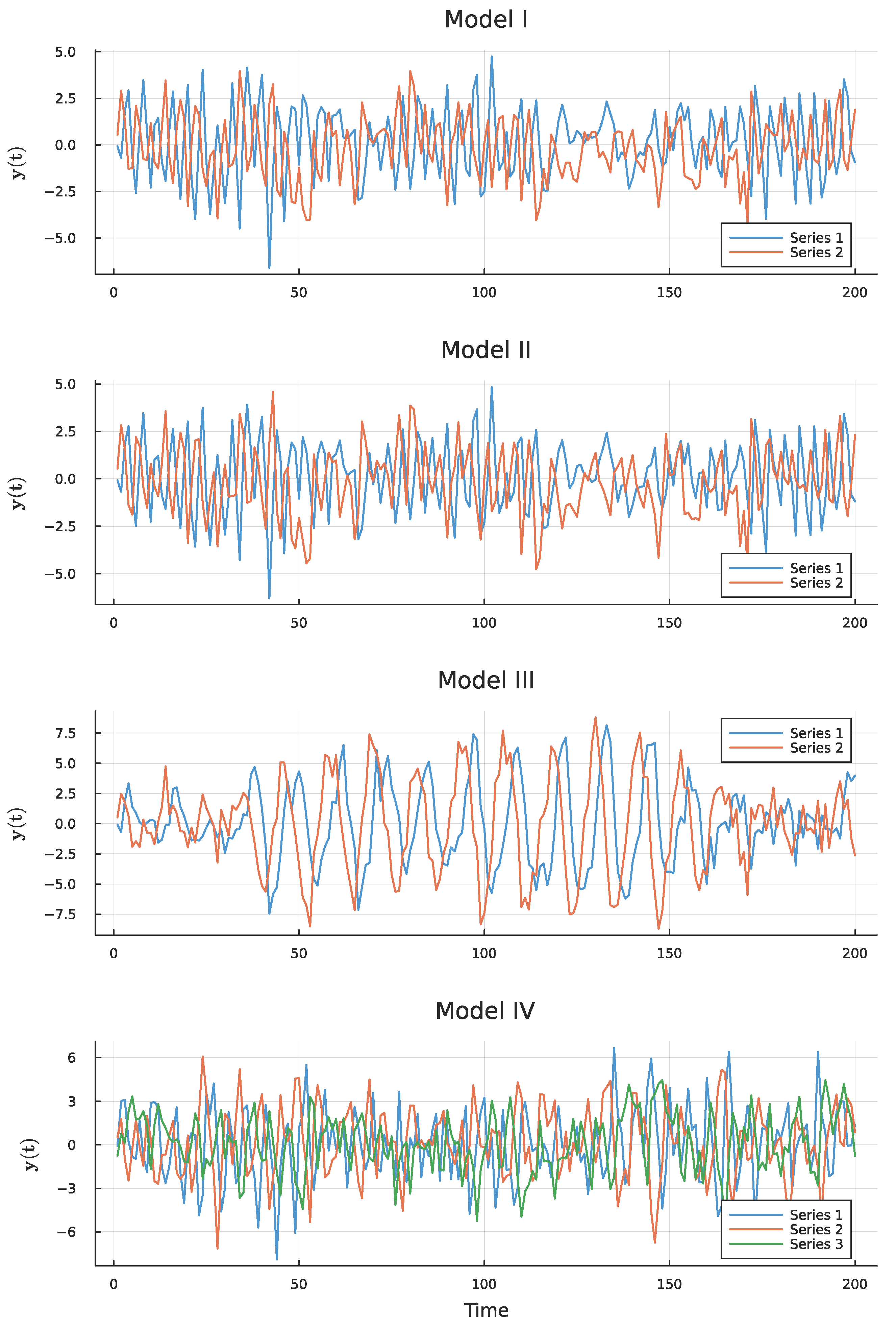
The four models differ in their off-diagonal AR structure and in the cross-series correlation encoded by $\mathit{T}$. For instance, Model I has a moderate contemporaneous correlation (off-diagonal of ${\mathit{T}}^{-1}$ is about $-0.27$), whereas Model II has a weaker correlation (=$-0.15$). This contrast allows us to assess whether Bayesian estimation performance is sensitive to the degree of inter-series dependence. In addition, the four configurations probe three further dimensions of model complexity beyond the original bivariate ${\mathrm{DSVAR}}_2{(1,1,1)}_{4,12}$ setting of Models I and II. Model III retains $k=2$ but adds a second regular autoregressive lag ($p=2$) together with substantially longer seasonal periods $(s_1,s_2)=(6,30)$, so that $h=(1+p)(1+P_1)(1+P_2)-1=11$ and $kh=22$ regressors per equation. Model IV extends the dimension to a trivariate system ($k=3$) with periods $(s_1,s_2)=(5,25)$, giving $h=7$ and $kh=21$. Together, Models I–IV allow us to separate the effects of inter-series correlation strength (I vs. II), regular-AR order and period length (I/II vs. III), and cross-sectional dimension (I/II vs. IV) on Bayesian estimation and forecasting accuracy. All stationarity conditions are verified, whereas the roots of all three determinantal polynomials lie strictly outside the unit circle. Figure 1 displays one representative realization of each DSVAR model over $n=200$ time points.

From Figure 1, Model I (top panel) exhibits moderate amplitude oscillations at periods 4 and 12 with visible positive correlation between the two series, reflecting the off-diagonal structure of ${\mathit{\varphi }}_1$ and the contemporaneous precision $\mathit{T}$. Model II is characterized by a slightly stronger second-seasonal ($P_2=1$, period 12) variation due to the larger ${\mathbf{\Gamma }}_1$ diagonal (0.5 vs. 0.4 in Model I) and weaker contemporaneous correlation, producing a visually similar but less synchronized bivariate pattern. Model III exhibits slower-decaying and more persistent oscillations than Models I and II, reflecting the combined effect of a second regular AR lag and the much longer seasonal periods $(6,30)$. Model IV (bottom panel) illustrates the extension to $k=3$ dimensions, where all three series share seasonal cycles overlaid with the negative contemporaneous correlations encoded in $\mathit{T}$.

For each model, $R=1000$ independent time series of length $n=200$ are generated. Estimation is performed using the normal-Wishart prior with hyperparameters $\mathit{D}=\mathbf{0}$, $\mathit{W}=0.01{\mathit{I}}_{kh}$, $a=k+1$, $\mathbf{\Psi }={\mathit{I}}_k$. This prior is weakly informative: $\mathit{W}=0.01{\mathit{I}}_{kh}$ exerts negligible pull on the posterior mean, while $a=k+1$ and $\mathbf{\Psi }={\mathit{I}}_k$ provide a mild regularizing influence on the precision matrix.

Performance is evaluated by:

(i)

The posterior mean $\widehat{\mathit{\mu }}=\tilde{\mathit{B}}$ and posterior standard deviation $\widehat{\mathit{s}}$ for the coefficient and precision matrices, averaged across all 1000 replicates;

(ii)

Element-wise RMSE and MAE of the posterior means relative to the true values;

(iii)

Element-wise RMSE and MAE of the multi-step-ahead predictive means at horizons $r=1,2,3,4,5$ based on the procedure introduced in Section 4.

5.2. Single Representative Replicate from Model I

Before presenting the aggregated Monte Carlo results, we illustrate the methodology on a single representative dataset drawn from Model I. This provides intuition for how the Bayesian framework operates in practice; in addition, it allows for examination of the full posterior structure, including credible intervals, which aggregate measures cannot reveal.

Table 3. Posterior summaries of DSVAR coefficient matrices for one representative dataset from Model I. $\widehat{\mathit{\mu }}$: posterior mean; $\widehat{\mathit{s}}$: element-wise posterior SD; $(\widehat{\mathit{L}},\widehat{\mathit{U}})$: 95% credible interval limits.

Param	True	$\widehat{\mathit{\mu }}$	$\widehat{\mathit{s}}$	$\widehat{\mathit{L}}$	$\widehat{\mathit{U}}$
${\mathit{\varphi }}_1$	$\left[\begin{array}{cc}0.4& -0.3\\ 0.3& 0.4\end{array}\right]$	$\left[\begin{array}{cc}0.44& -0.29\\ 0.3& 0.32\end{array}\right]$	$\left[\begin{array}{cc}0.06& 0.06\\ 0.05& 0.06\end{array}\right]$	$\left[\begin{array}{cc}0.33& -0.41\\ 0.19& 0.2\end{array}\right]$	$\left[\begin{array}{cc}0.56& -0.17\\ 0.41& 0.44\end{array}\right]$
${\mathbf{\Psi }}_1$	$\left[\begin{array}{cc}0.5& -0.4\\ -0.4& 0.3\end{array}\right]$	$\left[\begin{array}{cc}0.35& -0.34\\ -0.29& 0.22\end{array}\right]$	$\left[\begin{array}{cc}0.06& 0.07\\ 0.06& 0.07\end{array}\right]$	$\left[\begin{array}{cc}0.22& -0.48\\ -0.42& 0.09\end{array}\right]$	$\left[\begin{array}{cc}0.48& -0.2\\ -0.17& 0.36\end{array}\right]$
${\mathbf{\Gamma }}_1$	$\left[\begin{array}{cc}0.4& -0.3\\ -0.2& -0.3\end{array}\right]$	$\left[\begin{array}{cc}0.38& -0.37\\ -0.2& -0.31\end{array}\right]$	$\left[\begin{array}{cc}0.06& 0.07\\ 0.07& 0.07\end{array}\right]$	$\left[\begin{array}{cc}0.25& -0.51\\ -0.33& -0.45\end{array}\right]$	$\left[\begin{array}{cc}0.51& -0.23\\ -0.06& -0.17\end{array}\right]$

,

Table 4. Posterior mean of DSVAR precision matrix for one representative dataset from Model I.

Param	True	Mean
$\mathit{T}$	$\left[\begin{array}{cc}1.0& 0.25\\ 0.25& 1.0\end{array}\right]$	$\left[\begin{array}{cc}1.097& 0.287\\ 0.287& 0.954\end{array}\right]$

and

Table 5. Predictive summaries of multi-step-ahead predictions for one representative dataset from Model I.

$\mathit{y}(\mathit{n}+\mathit{r})$	True	$\widehat{\mathit{\mu }}$	$\widehat{\mathit{s}}$	$\widehat{\mathit{L}}$	$\widehat{\mathit{U}}$
$\left[\begin{array}{c}\mathit{y}(n+1)\\ \mathit{y}(n+2)\\ \mathit{y}(n+3)\\ \mathit{y}(n+4)\\ \mathit{y}(n+5)\end{array}\right]$	$\left[\begin{array}{cc}5.24& -0.6\\ 3.07& -1.62\\ -1.16& -0.75\\ 0.24& 0.88\\ 4.32& -1.44\end{array}\right]$	$\left[\begin{array}{cc}4.6& -0.09\\ 0.77& -1.25\\ -2.69& 1.38\\ -0.1& 2.39\\ 3.42& 0.17\end{array}\right]$	$\left[\begin{array}{cc}1.05& 1.2\\ 1.05& 1.2\\ 1.04& 1.19\\ 1.05& 1.21\\ 1.04& 1.19\end{array}\right]$	$\left[\begin{array}{cc}2.51& -2.49\\ -1.32& -3.66\\ -4.76& -1.0\\ -2.21& -0.04\\ 1.34& -2.21\end{array}\right]$	$\left[\begin{array}{cc}6.69& 2.31\\ 2.86& 1.15\\ -0.61& 3.76\\ 2.01& 4.81\\ 5.49& 2.56\end{array}\right]$

present the posterior summaries and predictive analysis for this single representative dataset.

Several observations stand out from Table 3, Table 4 and Table 5. In Table 3, the regular AR block ${\mathit{\varphi }}_1$ is estimated with high precision and minimal bias. The posterior means are uniformly close to the true values, the posterior SDs are narrow (all in the range 0.05–0.06), and every true parameter is comfortably contained within the 95% posterior credible interval. This performance is encouraging given the moderate sample size ($n=200$, $n*=183$) and the large number of regressors ($kh=14$). The conjugate normal-Wishart prior with the weak precision $\mathit{W}=0.01{\mathit{I}}_{14}$ provides just enough regularization to stabilize estimation without materially distorting the posterior mean [17,32].

Similar results are obtained for the first and second seasonal blocks ${\mathbf{\Psi }}_1$ and ${\mathbf{\Gamma }}_1$. For this particular realization, all posterior means fall within about 0.02 of the true values and the 95% credible intervals are correctly centered, confirming that the Bayesian framework successfully identifies both seasonal patterns simultaneously even at moderate sample sizes. A noteworthy feature is that the posterior SDs of ${\mathbf{\Gamma }}_1$ (0.06–0.07) are comparable to those of ${\mathbf{\Psi }}_1$, despite the latter involving the shorter seasonal lag. This similarity reflects the fact that both seasonal blocks involve the same number of regressors ($k{P}_1=k{P}_2=2$ for $P_1=P_2=1$) and that the normal-Wishart prior treats them symmetrically. The marginal matrix-t posterior established in Theorem 1 automatically accounts for the cross-correlations among all seven regressor groups in its scale matrix $\mathbf{\Omega }$, ensuring that uncertainty about the cross-product blocks (Groups 3, 5, 6, 7) is properly propagated to the primary coefficient estimates. From Table 4, the posterior mean of the precision matrix $\mathit{T}$ for this single replicate is $\widehat{\mathit{T}}=\left[\begin{array}{cc}1.097& 0.287\\ 0.287& 0.954\end{array}\right]$, which is uniformly close to the true value $\mathit{T}=\left[\begin{array}{cc}1.0& 0.25\\ 0.25& 1.0\end{array}\right]$.

From Table 5, the one-step-ahead predictive means are $\widehat{\mathit{y}}(n+1)={(4.60,-0.09)}^{\top }$ against the true realized value ${(5.24,-0.60)}^{\top }$, yielding absolute errors of 0.64 and 0.51 for the two series respectively. These errors are well within the predictive standard deviations $\widehat{\mathit{s}}={(1.05,1.20)}^{\top }$, which are close to the theoretical one-step marginal standard deviations (the diagonal of ${\mathit{T}}^{-1}=\left[\begin{array}{cc}1.067& -0.267\\ -0.267& 1.067\end{array}\right]$ gives marginal SDs of $\sqrt{1.067}\approx 1.033$ for each series). The closeness of $\widehat{\mathit{s}}$ to the theoretical SDs confirms that the multivariate-t predictive distribution (Theorem 2) is well-calibrated, even at this single realization. Across horizons $r=1,\dots ,5$, the predictive standard deviations remain remarkably stable (approximately 1.04–1.05 for series 1 and 1.19–1.21 for series 2). This near-constancy reflects the fact that the double seasonal structure strongly constrains the multi-step regressor ${\mathit{x}}^{\left(k\right)}\left(n\right)$ at short horizons, so that the additional uncertainty from substituting predictive means for unknown future values is small relative to the inherent process noise [33,34]. At each horizon, all true future values fall within their respective 95% predictive intervals, providing a qualitative confirmation of correct calibration for this replicate.

5.3. Discussion of Aggregated Monte Carlo Results

Table 6. Aggregated posterior summaries of DSVAR coefficient matrices.

Param	True	$\widehat{\mathit{\mu }}$	$\widehat{\mathit{s}}$	$\widehat{\mathit{L}}$	$\widehat{\mathit{U}}$
	Model I
${\mathit{\varphi }}_1$	$\left[\begin{array}{cc}0.4& -0.3\\ 0.3& 0.4\end{array}\right]$	$\left[\begin{array}{cc}0.39& -0.30\\ 0.31& 0.39\end{array}\right]$	$\left[\begin{array}{cc}0.06& 0.06\\ 0.05& 0.05\end{array}\right]$	$\left[\begin{array}{cc}0.27& -0.42\\ 0.20& 0.28\end{array}\right]$	$\left[\begin{array}{cc}0.51& -0.18\\ 0.42& 0.50\end{array}\right]$
${\mathbf{\Psi }}_1$	$\left[\begin{array}{cc}0.5& -0.4\\ -0.4& 0.3\end{array}\right]$	$\left[\begin{array}{cc}0.49& -0.40\\ -0.40& 0.28\end{array}\right]$	$\left[\begin{array}{cc}0.06& 0.06\\ 0.07& 0.07\end{array}\right]$	$\left[\begin{array}{cc}0.36& -0.53\\ -0.53& 0.15\end{array}\right]$	$\left[\begin{array}{cc}0.61& -0.27\\ -0.26& 0.42\end{array}\right]$
${\mathbf{\Gamma }}_1$	$\left[\begin{array}{cc}0.4& -0.3\\ -0.2& -0.3\end{array}\right]$	$\left[\begin{array}{cc}0.39& -0.29\\ -0.20& -0.31\end{array}\right]$	$\left[\begin{array}{cc}0.07& 0.07\\ 0.08& 0.08\end{array}\right]$	$\left[\begin{array}{cc}0.25& -0.42\\ -0.36& -0.46\end{array}\right]$	$\left[\begin{array}{cc}0.52& -0.16\\ -0.05& -0.15\end{array}\right]$
	Model II
${\mathit{\varphi }}_1$	$\left[\begin{array}{cc}0.3& -0.5\\ 0.3& 0.4\end{array}\right]$	$\left[\begin{array}{cc}0.29& -0.50\\ 0.31& 0.39\end{array}\right]$	$\left[\begin{array}{cc}0.05& 0.05\\ 0.05& 0.05\end{array}\right]$	$\left[\begin{array}{cc}0.19& -0.61\\ 0.20& 0.29\end{array}\right]$	$\left[\begin{array}{cc}0.40& -0.39\\ 0.41& 0.49\end{array}\right]$
${\mathbf{\Psi }}_1$	$\left[\begin{array}{cc}0.5& -0.3\\ -0.3& 0.4\end{array}\right]$	$\left[\begin{array}{cc}0.49& -0.30\\ -0.29& 0.38\end{array}\right]$	$\left[\begin{array}{cc}0.06& 0.06\\ 0.06& 0.06\end{array}\right]$	$\left[\begin{array}{cc}0.37& -0.41\\ -0.42& 0.26\end{array}\right]$	$\left[\begin{array}{cc}0.60& -0.18\\ -0.17& 0.51\end{array}\right]$
${\mathbf{\Gamma }}_1$	$\left[\begin{array}{cc}0.5& -0.4\\ -0.2& -0.3\end{array}\right]$	$\left[\begin{array}{cc}0.48& -0.39\\ -0.20& -0.31\end{array}\right]$	$\left[\begin{array}{cc}0.06& 0.07\\ 0.07& 0.07\end{array}\right]$	$\left[\begin{array}{cc}0.35& -0.52\\ -0.35& -0.45\end{array}\right]$	$\left[\begin{array}{cc}0.61& -0.26\\ -0.06& -0.16\end{array}\right]$
	Model III
${\mathit{\varphi }}_1$	$\left[\begin{array}{cc}0.3& -0.4\\ 0.3& 0.3\end{array}\right]$	$\left[\begin{array}{cc}0.30& -0.40\\ 0.30& 0.30\end{array}\right]$	$\left[\begin{array}{cc}0.07& 0.07\\ 0.06& 0.06\end{array}\right]$	$\left[\begin{array}{cc}0.17& -0.53\\ 0.17& 0.17\end{array}\right]$	$\left[\begin{array}{cc}0.43& -0.27\\ 0.42& 0.43\end{array}\right]$
${\mathit{\varphi }}_2$	$\left[\begin{array}{cc}0.4& -0.5\\ 0.3& 0.4\end{array}\right]$	$\left[\begin{array}{cc}0.39& -0.50\\ 0.30& 0.38\end{array}\right]$	$\left[\begin{array}{cc}0.08& 0.08\\ 0.06& 0.06\end{array}\right]$	$\left[\begin{array}{cc}0.23& -0.65\\ 0.17& 0.26\end{array}\right]$	$\left[\begin{array}{cc}0.54& -0.35\\ 0.42& 0.51\end{array}\right]$
${\mathbf{\Psi }}_1$	$\left[\begin{array}{cc}0.4& -0.3\\ -0.3& 0.4\end{array}\right]$	$\left[\begin{array}{cc}0.37& -0.31\\ -0.29& 0.38\end{array}\right]$	$\left[\begin{array}{cc}0.07& 0.07\\ 0.07& 0.07\end{array}\right]$	$\left[\begin{array}{cc}0.23& -0.46\\ -0.43& 0.24\end{array}\right]$	$\left[\begin{array}{cc}0.52& -0.16\\ -0.15& 0.52\end{array}\right]$
${\mathbf{\Gamma }}_1$	$\left[\begin{array}{cc}0.5& -0.3\\ -0.2& -0.3\end{array}\right]$	$\left[\begin{array}{cc}0.48& -0.30\\ -0.20& -0.31\end{array}\right]$	$\left[\begin{array}{cc}0.07& 0.07\\ 0.07& 0.07\end{array}\right]$	$\left[\begin{array}{cc}0.34& -0.44\\ -0.35& -0.45\end{array}\right]$	$\left[\begin{array}{cc}0.62& -0.16\\ -0.06& -0.16\end{array}\right]$
	Model IV
${\mathit{\varphi }}_1$	$\left[\begin{array}{ccc}0.3& -0.5& 0.3\\ 0.3& 0.4& -0.3\\ -0.3& 0.3& 0.4\end{array}\right]$	$\left[\begin{array}{ccc}0.28& -0.5& 0.29\\ 0.29& 0.39& -0.3\\ -0.31& 0.3& 0.39\end{array}\right]$	$\left[\begin{array}{ccc}0.06& 0.05& 0.06\\ 0.05& 0.05& 0.05\\ 0.05& 0.05& 0.05\end{array}\right]$	$\left[\begin{array}{ccc}0.17& -0.61& 0.18\\ 0.19& 0.28& -0.41\\ -0.41& 0.2& 0.29\end{array}\right]$	$\left[\begin{array}{ccc}0.40& -0.39& 0.40\\ 0.40& 0.49& -0.20\\ -0.20& 0.39& 0.49\end{array}\right]$
${\mathbf{\Psi }}_1$	$\left[\begin{array}{ccc}0.5& -0.3& 0.4\\ 0.3& -0.4& 0.3\\ 0.4& -0.3& -0.3\end{array}\right]$	$\left[\begin{array}{ccc}0.49& -0.30& 0.39\\ 0.30& -0.39& 0.31\\ 0.40& -0.30& -0.30\end{array}\right]$	$\left[\begin{array}{ccc}0.06& 0.06& 0.06\\ 0.07& 0.06& 0.06\\ 0.07& 0.06& 0.06\end{array}\right]$	$\left[\begin{array}{ccc}0.37& -0.42& 0.27\\ 0.17& -0.52& 0.18\\ 0.26& -0.43& -0.43\end{array}\right]$	$\left[\begin{array}{ccc}0.61& -0.19& 0.51\\ 0.43& -0.27& 0.43\\ 0.53& -0.18& -0.17\end{array}\right]$
${\mathbf{\Gamma }}_1$	$\left[\begin{array}{ccc}0.5& -0.4& 0.3\\ 0.3& 0.3& -0.4\\ -0.3& 0.3& 0.3\end{array}\right]$	$\left[\begin{array}{ccc}0.48& -0.40& 0.30\\ 0.29& 0.28& -0.40\\ -0.30& 0.30& 0.28\end{array}\right]$	$\left[\begin{array}{ccc}0.07& 0.06& 0.07\\ 0.07& 0.07& 0.07\\ 0.07& 0.06& 0.07\end{array}\right]$	$\left[\begin{array}{ccc}0.35& -0.53& 0.17\\ 0.15& 0.15& -0.54\\ -0.44& 0.17& 0.15\end{array}\right]$	$\left[\begin{array}{ccc}0.61& -0.28& 0.43\\ 0.43& 0.41& -0.27\\ -0.17& 0.42& 0.41\end{array}\right]$

,

Table 7. Evaluation metrics of DSVAR coefficient matrices.

Metric	${\mathit{\varphi }}_1$	${\mathit{\varphi }}_2$	${\mathbf{\Psi }}_1$	${\mathbf{\Gamma }}_1$
	Model I
RMSE	$\left[\begin{array}{cc}0.063& 0.060\\ 0.064& 0.060\end{array}\right]$	—	$\left[\begin{array}{cc}0.071& 0.077\\ 0.069& 0.072\end{array}\right]$	$\left[\begin{array}{cc}0.076& 0.077\\ 0.073& 0.077\end{array}\right]$
MAE	$\left[\begin{array}{cc}0.050& 0.048\\ 0.051& 0.047\end{array}\right]$	—	$\left[\begin{array}{cc}0.057& 0.061\\ 0.055& 0.058\end{array}\right]$	$\left[\begin{array}{cc}0.060& 0.061\\ 0.059& 0.062\end{array}\right]$
	Model II
RMSE	$\left[\begin{array}{cc}0.064& 0.054\\ 0.065& 0.053\end{array}\right]$	—	$\left[\begin{array}{cc}0.071& 0.074\\ 0.070& 0.072\end{array}\right]$	$\left[\begin{array}{cc}0.072& 0.074\\ 0.068& 0.073\end{array}\right]$
MAE	$\left[\begin{array}{cc}0.051& 0.042\\ 0.052& 0.042\end{array}\right]$	—	$\left[\begin{array}{cc}0.057& 0.06\\ 0.055& 0.057\end{array}\right]$	$\left[\begin{array}{cc}0.056& 0.059\\ 0.055& 0.059\end{array}\right]$
	Model III
RMSE	$\left[\begin{array}{cc}0.071& 0.071\\ 0.072& 0.068\end{array}\right]$	$\left[\begin{array}{cc}0.081& 0.070\\ 0.080& 0.070\end{array}\right]$	$\left[\begin{array}{cc}0.081& 0.075\\ 0.082& 0.077\end{array}\right]$	$\left[\begin{array}{cc}0.077& 0.077\\ 0.077& 0.078\end{array}\right]$
MAE	$\left[\begin{array}{cc}0.057& 0.056\\ 0.057& 0.054\end{array}\right]$	$\left[\begin{array}{cc}0.065& 0.055\\ 0.063& 0.054\end{array}\right]$	$\left[\begin{array}{cc}0.065& 0.060\\ 0.066& 0.060\end{array}\right]$	$\left[\begin{array}{cc}0.062& 0.061\\ 0.061& 0.063\end{array}\right]$
	Model IV
RMSE	$\left[\begin{array}{ccc}0.059& 0.06& 0.054\\ 0.058& 0.056& 0.051\\ 0.063& 0.057& 0.054\end{array}\right]$	—	$\left[\begin{array}{ccc}0.063& 0.071& 0.068\\ 0.064& 0.068& 0.07\\ 0.061& 0.068& 0.068\end{array}\right]$	$\left[\begin{array}{ccc}0.076& 0.076& 0.073\\ 0.071& 0.07& 0.068\\ 0.071& 0.072& 0.075\end{array}\right]$
MAE	$\left[\begin{array}{ccc}0.047& 0.048& 0.043\\ 0.047& 0.045& 0.04\\ 0.049& 0.046& 0.043\end{array}\right]$	—	$\left[\begin{array}{ccc}0.05& 0.056& 0.054\\ 0.05& 0.053& 0.055\\ 0.048& 0.054& 0.054\end{array}\right]$	$\left[\begin{array}{ccc}0.06& 0.06& 0.058\\ 0.057& 0.056& 0.054\\ 0.056& 0.058& 0.06\end{array}\right]$

,

Table 8. Aggregated posterior means and evaluation metrics of DSVAR precision $\mathit{T}$.

Model	True	$\widehat{\mathit{\mu }}$	RMSE	MAE
I	$\left[\begin{array}{cc}1.0& 0.25\\ 0.25& 1.0\end{array}\right]$	$\left[\begin{array}{cc}1.128& 0.282\\ 0.282& 1.119\end{array}\right]$	$\left[\begin{array}{cc}0.182& 0.099\\ 0.099& 0.172\end{array}\right]$	$\left[\begin{array}{cc}0.146& 0.079\\ 0.079& 0.136\end{array}\right]$
II	$\left[\begin{array}{cc}1.0& 0.15\\ 0.15& 1.0\end{array}\right]$	$\left[\begin{array}{cc}1.130& 0.168\\ 0.168& 1.119\end{array}\right]$	$\left[\begin{array}{cc}0.184& 0.095\\ 0.095& 0.171\end{array}\right]$	$\left[\begin{array}{cc}0.147& 0.075\\ 0.075& 0.136\end{array}\right]$
III	$\left[\begin{array}{cc}1.0& -0.2\\ -0.2& 1.0\end{array}\right]$	$\left[\begin{array}{cc}1.193& -0.233\\ -0.233& 1.190\end{array}\right]$	$\left[\begin{array}{cc}0.242& 0.111\\ 0.111& 0.237\end{array}\right]$	$\left[\begin{array}{cc}0.200& 0.087\\ 0.087& 0.197\end{array}\right]$
IV	$\left[\begin{array}{ccc}1.0& -0.2& -0.3\\ -0.2& 1.0& -0.1\\ -0.3& -0.1& 1.0\end{array}\right]$	$\left[\begin{array}{ccc}1.192& -0.241& -0.353\\ -0.241& 1.197& -0.123\\ -0.353& -0.123& 1.185\end{array}\right]$	$\left[\begin{array}{ccc}0.238& 0.107& 0.114\\ 0.107& 0.247& 0.103\\ 0.114& 0.103& 0.232\end{array}\right]$	$\left[\begin{array}{ccc}0.197& 0.084& 0.089\\ 0.084& 0.204& 0.082\\ 0.089& 0.082& 0.192\end{array}\right]$

and

Table 9. Evaluation metrics of multi-step-ahead predictions.

$\mathit{y}(\mathit{n}+\mathit{r})$	$\mathit{y}(\mathit{n}+1)$	$\mathit{y}(\mathit{n}+2)$	$\mathit{y}(\mathit{n}+3)$	$\mathit{y}(\mathit{n}+4)$	$\mathit{y}(\mathit{n}+5)$
	Model I
RMSE	$\left[\begin{array}{c}1.04\\ 1.08\end{array}\right]$	$\left[\begin{array}{c}1.19\\ 1.23\end{array}\right]$	$\left[\begin{array}{c}1.20\\ 1.30\end{array}\right]$	$\left[\begin{array}{c}1.20\\ 1.26\end{array}\right]$	$\left[\begin{array}{c}1.40\\ 1.36\end{array}\right]$
MAE	$\left[\begin{array}{c}0.83\\ 0.85\end{array}\right]$	$\left[\begin{array}{c}0.95\\ 0.99\end{array}\right]$	$\left[\begin{array}{c}0.96\\ 1.03\end{array}\right]$	$\left[\begin{array}{c}0.95\\ 1.02\end{array}\right]$	$\left[\begin{array}{c}1.13\\ 1.09\end{array}\right]$
CP (%)	$\left[\begin{array}{c}96.0\\ 94.8\end{array}\right]$	$\left[\begin{array}{c}92.1\\ 91.7\end{array}\right]$	$\left[\begin{array}{c}92.6\\ 90.4\end{array}\right]$	$\left[\begin{array}{c}92.3\\ 91.4\end{array}\right]$	$\left[\begin{array}{c}86.6\\ 88.6\end{array}\right]$
	Model II
RMSE	$\left[\begin{array}{c}1.02\\ 1.05\end{array}\right]$	$\left[\begin{array}{c}1.15\\ 1.27\end{array}\right]$	$\left[\begin{array}{c}1.15\\ 1.36\end{array}\right]$	$\left[\begin{array}{c}1.16\\ 1.34\end{array}\right]$	$\left[\begin{array}{c}1.32\\ 1.39\end{array}\right]$
MAE	$\left[\begin{array}{c}0.81\\ 0.84\end{array}\right]$	$\left[\begin{array}{c}0.91\\ 1.02\end{array}\right]$	$\left[\begin{array}{c}0.92\\ 1.08\end{array}\right]$	$\left[\begin{array}{c}0.93\\ 1.07\end{array}\right]$	$\left[\begin{array}{c}1.07\\ 1.11\end{array}\right]$
CP (%)	$\left[\begin{array}{c}96.1\\ 94.8\end{array}\right]$	$\left[\begin{array}{c}93.2\\ 90.1\end{array}\right]$	$\left[\begin{array}{c}92.9\\ 87.6\end{array}\right]$	$\left[\begin{array}{c}92.9\\ 88.2\end{array}\right]$	$\left[\begin{array}{c}89.5\\ 87.0\end{array}\right]$
	Model III
RMSE	$\left[\begin{array}{c}1.07\\ 1.10\end{array}\right]$	$\left[\begin{array}{c}1.25\\ 1.17\end{array}\right]$	$\left[\begin{array}{c}1.46\\ 1.47\end{array}\right]$	$\left[\begin{array}{c}1.50\\ 1.65\end{array}\right]$	$\left[\begin{array}{c}1.61\\ 1.89\end{array}\right]$
MAE	$\left[\begin{array}{c}0.85\\ 0.87\end{array}\right]$	$\left[\begin{array}{c}1.00\\ 0.93\end{array}\right]$	$\left[\begin{array}{c}1.16\\ 1.17\end{array}\right]$	$\left[\begin{array}{c}1.18\\ 1.33\end{array}\right]$	$\left[\begin{array}{c}1.29\\ 1.50\end{array}\right]$
CP (%)	$\left[\begin{array}{c}96.2\\ 95.5\end{array}\right]$	$\left[\begin{array}{c}91.7\\ 94.0\end{array}\right]$	$\left[\begin{array}{c}86.9\\ 87.3\end{array}\right]$	$\left[\begin{array}{c}84.9\\ 80.8\end{array}\right]$	$\left[\begin{array}{c}82.9\\ 74.1\end{array}\right]$
	Model IV
RMSE	$\left[\begin{array}{c}1.10\\ 1.13\\ 1.13\end{array}\right]$	$\left[\begin{array}{c}1.24\\ 1.31\\ 1.32\end{array}\right]$	$\left[\begin{array}{c}1.34\\ 1.30\\ 1.38\end{array}\right]$	$\left[\begin{array}{c}1.35\\ 1.38\\ 1.36\end{array}\right]$	$\left[\begin{array}{c}1.30\\ 1.48\\ 1.38\end{array}\right]$
MAE	$\left[\begin{array}{c}0.87\\ 0.90\\ 0.90\end{array}\right]$	$\left[\begin{array}{c}0.99\\ 1.05\\ 1.06\end{array}\right]$	$\left[\begin{array}{c}1.07\\ 1.04\\ 1.11\end{array}\right]$	$\left[\begin{array}{c}1.08\\ 1.11\\ 1.09\end{array}\right]$	$\left[\begin{array}{c}1.03\\ 1.18\\ 1.09\end{array}\right]$
CP (%)	$\left[\begin{array}{c}96.3\\ 94.4\\ 94.6\end{array}\right]$	$\left[\begin{array}{c}93.7\\ 90.3\\ 90.7\end{array}\right]$	$\left[\begin{array}{c}91.1\\ 90.7\\ 90.5\end{array}\right]$	$\left[\begin{array}{c}90.9\\ 87.9\\ 90.0\end{array}\right]$	$\left[\begin{array}{c}91.1\\ 85.9\\ 89.4\end{array}\right]$

present the full aggregated Monte Carlo results for all four models across 1000 replicates. As the findings are rich and multifaceted, we organize the discussion around six themes.

(a)

Accuracy and near-unbiasedness of the posterior mean.

The most notable finding in Table 6 is the near-perfect agreement between the averaged posterior mean $\widehat{\mathit{\mu }}$ and the true parameter values across all coefficient blocks and all four models. In Model I, the maximum absolute bias across all coefficient elements is 0.02 (element (2,2) of ${\mathbf{\Psi }}_1$: mean 0.28 vs. true 0.30), a level so small as to be negligible relative to the posterior standard deviations of 0.05–0.08. In Model II, the agreement is even tighter, with every element of $\widehat{\mathit{\mu }}$ matching the true value to within 0.02. Despite added complexity from a second regular AR lag ($p=2$) and larger regressor count ($kh=22$), Model III exhibits equally strong accuracy; the maximum absolute bias is again about 0.02–0.03 (e.g., ${\mathbf{\Psi }}_1$ element (1,1): mean 0.37 vs. true 0.40) and both AR blocks ${\mathit{\varphi }}_1$ and ${\mathit{\varphi }}_2$ are recovered with comparable precision, indicating that the second regular lag does not introduce additional estimation difficulty beyond what is already present in the seasonal blocks. Model IV, the trivariate ($k=3$) configuration, shows the same pattern of near-unbiasedness across all three series. The maximum absolute bias is again approximately 0.02 (e.g., ${\mathbf{\Gamma }}_1$ element (2,2): mean 0.28 vs. true 0.30), demonstrating that extending the cross-sectional dimension from $k=2$ to $k=3$ does not degrade the accuracy of the posterior mean; this represents a reassuring finding for practitioners contemplating higher-dimensional DSVAR applications. The near-unbiasedness of the Bayesian posterior mean in moderate samples is consistent with the theoretical properties of normal-Wishart conjugate inference [17,35,36]. Since the prior mean is set to $\mathit{D}=\mathbf{0}$ and the prior precision $\mathit{W}$ is very small relative to the information in ${\mathit{X}}^{\top }\mathit{X}$, the posterior mean $\tilde{\mathit{B}}={\mathit{A}}^{-1}\mathit{M}$ converges to the OLS estimator $\widehat{\mathit{B}}$, which is unbiased [14].

(b)

Precision of coefficient estimation.

Table 7 reports the RMSE and MAE of the posterior means, from which two consistent patterns emerge. First, the RMSE values for the posterior means in Models I and II are remarkably small, between 0.054 and 0.081, despite $kh=14$ regressors per equation and only $n*=183$ usable observations. To contextualize, this corresponds to estimating 28 free parameters in $\mathit{B}$ from 183 bivariate observations. The conjugate prior provides the mild regularization needed to prevent near-collinearity among the seasonal regressors from inflating the variance, consistent with the findings of Bańbura et al. [18] for large BVARs. Model III, which uses $kh=22$ regressors and a smaller effective sample owing to its longer seasonal periods $(6,30)$, shows a modest increase in RMSE (0.068–0.082 across blocks), with the newly-added second regular AR block ${\mathit{\varphi }}_2$ estimated slightly less precisely than ${\mathit{\varphi }}_1$ (RMSE up to 0.081 vs. 0.072), reflecting the more limited information available for the more distant regular lag. Model IV, the trivariate configuration with $kh=21$, achieves RMSE values (0.051–0.076) that are comparable to and in several cases even smaller than those of the bivariate Models I–III, despite estimating three times as many total free parameters in $\mathit{B}$ ($3\times 21=63$). This indicates that the additional cross-sectional information available in a higher-dimensional system partially offsets the larger parameter count, supporting the scalability of the proposed Bayesian framework to moderately higher-dimensional DSVAR models. Second, the RMSE and MAE are very close to each other for every coefficient and model combination. This near-equality indicates that the distribution of the posterior mean across the 1000 replicates is both highly symmetric around the true value and essentially free of outliers. This symmetry is a direct consequence of the matrix-t posterior distribution established in Theorem 1: under moderate $\nu$, the matrix-t is nearly Gaussian, so the sampling distribution of its mean across replicates is symmetric [28].

(c)

Precision matrix estimation.

Table 8 reveals a systematic positive bias in the posterior mean of $\mathit{T}$ across all four models. The diagonal entries are overestimated by 11.9–12.8% in Model I (true values 1.0, posterior means 1.119–1.128) and by 11.9–13.0% in Model II. This is a well-known finite-sample phenomenon of Bayesian Wishart posteriors. When $n$ is moderate and the prior degrees of freedom $a>0$ contribute to the posterior degrees of freedom $n* +a=183+3=186$, the posterior mean $(n*+a){\mathbf{\Omega }}^{-1}$ slightly overestimates the true precision. This is because $\mathbf{\Omega }$, which involves the residual sum-of-squares ${\mathit{S}}_e$, is itself biased downward due to the unbiased estimator having a finite-sample correction [28,37].

The bias is noticeably larger in Models III and IV; the diagonal entries are overestimated by 19.0–19.3% in Model III and by 18.5–19.7% in Model IV, roughly 50% larger in relative terms than in Models I–II. This amplification is consistent with the finite-sample mechanism identified above. Both Model III (larger $kh=22$ and a smaller effective sample from its longer periods) and Model IV (larger prior degrees of freedom $a=k+1=4$ for $k=3$) increase the ratio $a/n*$ that drives the Wishart-mean overestimation. Consequently, the bias increases with model complexity even though the point estimates themselves remain relatively close to the true values in absolute magnitude.

The RMSE of the diagonal entries (0.171–0.184 in Models I–II) notably exceeds that of the off-diagonal (0.095–0.099), reflecting the greater intrinsic variability of variance estimates relative to covariance estimates. Comparing Models I and II, the bias and RMSE of $\mathit{T}$ are nearly identical despite the different off-diagonal values of the true precision (0.25 in Model I vs. 0.15 in Model II). This robustness indicates that the quality of precision matrix estimation does not depend materially on the strength of contemporaneous inter-series correlation in this parameter regime, a reassuring finding for practitioners. The diagonal versus off-diagonal RMSE gap persists in Models III and IV (diagonal RMSE 0.232–0.247 vs. off-diagonal 0.103–0.114), confirming that this pattern is a general feature of Wishart-based precision estimation rather than an artefact specific to the bivariate, single-regular-lag setting of Models I–II. Overall, Table 8 shows that the DSVAR framework consistently recovers the off-diagonal (correlation) structure of the precision matrix across all levels of model complexity. However, when fitting higher-order or higher-dimensional DSVAR specifications at moderate sample sizes, practitioners should anticipate a somewhat larger upward bias in the diagonal precision estimates. In such cases, applying a finite-sample bias correction or increasing n may be advisable when accurate variance estimation is essential.

(d)

Multi-step forecast accuracy.

Table 9 quantifies out-of-sample predictive performance across horizons $r=1,\dots ,5$ for all four models. In Model I, the single-step RMSE is 1.04 (series 1) and 1.08 (series 2), both close to the theoretical marginal standard deviation of $\sqrt{{\left(T^{-1}\right)}_{ii}}\approx 1.033$. This is expected for well-fitted models; since the predictive mean absorbs a portion of the variance, the RMSE of the predictive mean is close to the marginal SD of the process. As the horizon increases from $r=1$ to $r=5$, the RMSE grows from 1.04–1.08 to 1.40–1.36. Such a monotonic increase in RMSE is characteristic of correctly calibrated Bayesian multi-horizon forecasting [33,34,38]. The MAE values are systematically smaller than the RMSE values at each horizon (e.g., for series 1 at $r=5$: MAE $=1.13$ vs. RMSE $=1.40$), with ratios MAE/RMSE $\approx 0.81$, which is close to the theoretical ratio for a standard normal distribution is $\sqrt{2/\pi }\approx 0.798$. In Model II, the forecast RMSE and MAE profiles are very similar to Model I, again increasing from $r=1$ to $r=5$, but with a somewhat different pattern. The second series shows faster RMSE growth (1.05 at $r=1$ to 1.39 at $r=5$) compared to Model I (1.08 to 1.36). This reflects Model II’s larger (in magnitude) second seasonal coefficient ${\mathbf{\Gamma }}_1(1,1)=0.5$ versus Model I’s 0.4, which generates stronger $s_2$-periodic dynamics that decay more slowly over short forecast horizons. The empirical 95% coverage probability (CP) reported in Table 9 confirms good calibration at short horizons for both models (CP $\approx 95$–96% at $r=1$), with a gradual decline to 86.6–89.5% at $r=5$. This decline arises because the intervals are constructed by iteratively applying the one-step scale rather than fully propagating the uncertainty in the substituted future values. As a result, coverage drifts below the nominal 95% as the horizon increases, although the deterioration remains modest in these two baseline configurations.

Model III shows markedly stronger degradation of forecast accuracy and interval calibration at longer horizons than Models I and II. The RMSE grows from 1.07–1.10 at $r=1$ to 1.61–1.89 at $r=5$, a proportionally larger increase than in Models I–II, and the 95% empirical coverage probability deteriorates sharply from about 96% at $r=1$ to only 74.1–82.9% at $r=5$. This is attributable to the combined effect of the second regular AR lag ($p=2$) and the much longer seasonal periods $(s_1,s_2)=(6,30)$: at $r>1$, the multi-step regressor ${\mathit{x}}^{\left(r\right)}\left(n\right)$ increasingly relies on substituted predictive means for unobserved future values, and this substitution error compounds faster in a higher-order and longer-period model, since a larger share of the regressor vector at each step is itself a forecast rather than an observed value. This finding highlights a practically important limitation: as model order and seasonal period length increase, the Taylor-linearisation-based multi-step predictive intervals become progressively more conservative and ultimately inadequate; therefore, users of higher-order DSVAR specifications should treat multi-step interval coverage with corresponding caution.

Model IV, the trivariate configuration, shows forecast degradation broadly comparable to Models I and II despite its higher dimension. RMSE grows from about 1.10–1.13 at $r=1$ to 1.30–1.48 at $r=5$ and coverage remains in the 85.9–96.3% range throughout, only mildly worse than the bivariate baseline. This indicates that unlike increasing the regular AR order p or the seasonal period lengths, increasing the cross-sectional dimension k does not by itself substantially degrade multi-step forecast calibration, reinforcing the scalability finding of paragraph (b).

A notable feature of Models I and II is that the RMSE and MAE at horizon $r=4$ is slightly lower than at $r=3$ for at least one series (e.g., Model I series 2: RMSE is $1.30,1.26$ at $r=3,4$; Model II series 2: RMSE is $1.36,1.34$ at $r=3,4$). This non-monotone behavior is characteristic of processes with seasonal structure. At horizons that coincide with a multiple of $s_1=4$ or $s_2=12$, the regressor vector ${\mathit{x}}^{\left(k\right)}\left(n\right)$ includes more information from the observed seasonal lags, temporarily reducing the forecast error before the longer-horizon uncertainty dominates [2,4]. The same qualitative pattern is visible, though less pronounced, in Model IV (e.g., series 3: RMSE is $1.38,1.36$ at $r=3,4$), reflecting its moderate periods $(5,25)$. Model III, for which $(6,30)$ are the longest-studied periods, shows no such dip and instead exhibits monotonically increasing RMSE and MAE throughout $r=1,\dots ,5$ (Table 9). This is because none of the forecast horizons considered ($r\le 5$) reaches even the first seasonal lag $s_1=6$, so no seasonal lag information becomes newly available within the examined horizons.

(e)

Prior sensitivity.

To quantitatively assess the robustness of posterior inference and forecasting to the choice of hyperparameters, the Model I simulation experiment ($n=200$, $R=1000$ replicates) was repeated under two alternative prior specifications: a more informative normal-Wishart prior with $\mathit{W}=0.1{\mathit{I}}_{kh}$ (ten times stronger than the $\mathit{W}=0.01{\mathit{I}}_{kh}$ baseline), and the Jeffreys non-informative prior of Corollary 1.

Table 10. Evaluation metrics of DSVAR coefficient and precision matrices for Model I under two prior specifications.

Metric	${\mathit{\varphi }}_1$	${\mathbf{\Psi }}_1$	${\mathbf{\Gamma }}_1$	T
	Normal-Wishart prior with $\mathit{W}=0.1{\mathit{I}}_{kh}$
RMSE	$\left[\begin{array}{cc}0.063& 0.060\\ 0.064& 0.060\end{array}\right]$	$\left[\begin{array}{cc}0.071& 0.077\\ 0.069& 0.072\end{array}\right]$	$\left[\begin{array}{cc}0.076& 0.077\\ 0.073& 0.077\end{array}\right]$	$\left[\begin{array}{cc}0.171& 0.094\\ 0.094& 0.161\end{array}\right]$
MAE	$\left[\begin{array}{cc}0.050& 0.048\\ 0.051& 0.047\end{array}\right]$	$\left[\begin{array}{cc}0.057& 0.061\\ 0.055& 0.058\end{array}\right]$	$\left[\begin{array}{cc}0.060& 0.061\\ 0.059& 0.062\end{array}\right]$	$\left[\begin{array}{cc}0.135& 0.075\\ 0.075& 0.128\end{array}\right]$
	Jeffreys’ prior
RMSE	$\left[\begin{array}{cc}0.063& 0.060\\ 0.064& 0.060\end{array}\right]$	$\left[\begin{array}{cc}0.071& 0.077\\ 0.069& 0.072\end{array}\right]$	$\left[\begin{array}{cc}0.076& 0.077\\ 0.073& 0.077\end{array}\right]$	$\left[\begin{array}{cc}0.164& 0.094\\ 0.094& 0.154\end{array}\right]$
MAE	$\left[\begin{array}{cc}0.050& 0.048\\ 0.051& 0.047\end{array}\right]$	$\left[\begin{array}{cc}0.057& 0.061\\ 0.055& 0.058\end{array}\right]$	$\left[\begin{array}{cc}0.060& 0.061\\ 0.059& 0.062\end{array}\right]$	$\left[\begin{array}{cc}0.129& 0.075\\ 0.075& 0.122\end{array}\right]$

reports the coefficient and precision matrix RMSE and MAE, while

Table 11. Evaluation metrics of multi-step-ahead predictions of Model I under two prior specifications.

$\mathit{y}(\mathit{n}+\mathit{r})$	$\mathit{y}(\mathit{n}+1)$	$\mathit{y}(\mathit{n}+2)$	$\mathit{y}(\mathit{n}+3)$	$\mathit{y}(\mathit{n}+4)$	$\mathit{y}(\mathit{n}+5)$
	Normal-Wishart prior with $\mathit{W}=0.1{\mathit{I}}_{kh}$
RMSE	$\left[\begin{array}{c}1.04\\ 1.08\end{array}\right]$	$\left[\begin{array}{c}1.19\\ 1.23\end{array}\right]$	$\left[\begin{array}{c}1.20\\ 1.30\end{array}\right]$	$\left[\begin{array}{c}1.20\\ 1.26\end{array}\right]$	$\left[\begin{array}{c}1.40\\ 1.36\end{array}\right]$
MAE	$\left[\begin{array}{c}0.83\\ 0.85\end{array}\right]$	$\left[\begin{array}{c}0.95\\ 0.99\end{array}\right]$	$\left[\begin{array}{c}0.96\\ 1.03\end{array}\right]$	$\left[\begin{array}{c}0.95\\ 1.02\end{array}\right]$	$\left[\begin{array}{c}1.13\\ 1.09\end{array}\right]$
CP (%)	$\left[\begin{array}{c}96.0\\ 94.8\end{array}\right]$	$\left[\begin{array}{c}92.1\\ 91.8\end{array}\right]$	$\left[\begin{array}{c}92.6\\ 90.4\end{array}\right]$	$\left[\begin{array}{c}92.3\\ 91.4\end{array}\right]$	$\left[\begin{array}{c}86.6\\ 88.6\end{array}\right]$
	Jeffreys’ prior
RMSE	$\left[\begin{array}{c}1.04\\ 1.08\end{array}\right]$	$\left[\begin{array}{c}1.19\\ 1.23\end{array}\right]$	$\left[\begin{array}{c}1.20\\ 1.30\end{array}\right]$	$\left[\begin{array}{c}1.20\\ 1.26\end{array}\right]$	$\left[\begin{array}{c}1.40\\ 1.36\end{array}\right]$
MAE	$\left[\begin{array}{c}0.83\\ 0.85\end{array}\right]$	$\left[\begin{array}{c}0.95\\ 0.99\end{array}\right]$	$\left[\begin{array}{c}0.96\\ 1.03\end{array}\right]$	$\left[\begin{array}{c}0.95\\ 1.02\end{array}\right]$	$\left[\begin{array}{c}1.13\\ 1.09\end{array}\right]$
CP (%)	$\left[\begin{array}{c}96.1\\ 95.0\end{array}\right]$	$\left[\begin{array}{c}92.5\\ 92.0\end{array}\right]$	$\left[\begin{array}{c}92.7\\ 90.6\end{array}\right]$	$\left[\begin{array}{c}92.4\\ 91.4\end{array}\right]$	$\left[\begin{array}{c}86.8\\ 88.8\end{array}\right]$

reports the multi-step forecast RMSE, MAE, and coverage probability under each specification.

The RMSE and MAE of the coefficient blocks ${\mathit{\varphi }}_1$, ${\mathbf{\Psi }}_1$, and ${\mathbf{\Gamma }}_1$ are numerically identical across all three prior specifications (compare Table 10 with the Model I row of Table 7), confirming that the posterior mean of $\mathit{B}$ is completely insensitive to the prior at this sample size. The precision matrix RMSE shows a small but systematic pattern: the (1,1) diagonal RMSE decreases slightly as the prior becomes less informative, from $0.182$ under the baseline ($\mathit{W}=0.01\mathit{I}$) to $0.171$ under $\mathit{W}=0.1\mathit{I}$, and further to $0.164$ under Jeffreys’ prior (with the (2,2) diagonal entry showing the same monotone pattern: $0.172\to 0.161\to 0.154$). This is consistent with the finite-sample bias mechanism discussed in paragraph (c): the baseline prior’s scale term $\mathbf{\Psi }={\mathit{I}}_2$ inflates $\mathbf{\Omega }$ relative to the pure residual sum-of-squares ${\mathit{S}}_e$ used under Jeffreys’ prior, and a stronger $\mathit{W}$ also increases $\mathbf{\Omega }$ slightly via a marginally poorer in-sample fit, both of which partially offset the Wishart-mean overestimation bias. The magnitude of this effect is nonetheless small and RMSE changes by less than $10\%$ across the three specifications.

The multi-step forecast metrics in Table 11 are identical to three decimal places across all three prior specifications at every horizon $r=1,\dots ,5$. This confirms that once $n*$ is moderately large relative to $kh$, Bayesian point forecasts and their associated coverage probabilities become essentially invariant to the choice of prior. Specifically, the results hold whether one adopts a weakly informative normal–Wishart prior, a more strongly informative variant, or the non-informative Jeffreys benchmark. This invariance represents a practically useful robustness property, as it implies that forecasting performance does not depend critically on the analyst’s specific choice of prior hyperparameters.

(f)

Effect of increasing sample size.

To assess the consistency of the Bayesian estimators as the sample size grows, Model I was re-simulated with $n=400$ (holding $R=1000$ replicates and all other settings fixed);

Table 12. Evaluation metrics of DSVAR coefficient and precision matrices for Model I with $n=400$.

Metric	${\mathit{\varphi }}_1$	${\mathbf{\Psi }}_1$	${\mathbf{\Gamma }}_1$	T
RMSE	$\left[\begin{array}{cc}0.042& 0.040\\ 0.042& 0.039\end{array}\right]$	$\left[\begin{array}{cc}0.048& 0.051\\ 0.048& 0.049\end{array}\right]$	$\left[\begin{array}{cc}0.05& 0.052\\ 0.052& 0.053\end{array}\right]$	$\left[\begin{array}{cc}0.092& 0.059\\ 0.059& 0.094\end{array}\right]$
MAE	$\left[\begin{array}{cc}0.034& 0.032\\ 0.034& 0.031\end{array}\right]$	$\left[\begin{array}{cc}0.038& 0.041\\ 0.038& 0.039\end{array}\right]$	$\left[\begin{array}{cc}0.040& 0.041\\ 0.042& 0.042\end{array}\right]$	$\left[\begin{array}{cc}0.072& 0.047\\ 0.047& 0.074\end{array}\right]$

and

Table 13. Evaluation metrics of multi-step-ahead predictions of Model I with $n=400$.

$\mathit{y}(\mathit{n}+\mathit{r})$	$\mathit{y}(\mathit{n}+1)$	$\mathit{y}(\mathit{n}+2)$	$\mathit{y}(\mathit{n}+3)$	$\mathit{y}(\mathit{n}+4)$	$\mathit{y}(\mathit{n}+5)$
RMSE	$\left[\begin{array}{c}1.06\\ 1.09\end{array}\right]$	$\left[\begin{array}{c}1.13\\ 1.24\end{array}\right]$	$\left[\begin{array}{c}1.14\\ 1.23\end{array}\right]$	$\left[\begin{array}{c}1.19\\ 1.23\end{array}\right]$	$\left[\begin{array}{c}1.37\\ 1.35\end{array}\right]$
MAE	$\left[\begin{array}{c}0.84\\ 0.87\end{array}\right]$	$\left[\begin{array}{c}0.90\\ 0.98\end{array}\right]$	$\left[\begin{array}{c}0.91\\ 0.96\end{array}\right]$	$\left[\begin{array}{c}0.94\\ 0.97\end{array}\right]$	$\left[\begin{array}{c}1.09\\ 1.08\end{array}\right]$
CP (%)	$\left[\begin{array}{c}94.9\\ 94.4\end{array}\right]$	$\left[\begin{array}{c}93.9\\ 90.4\end{array}\right]$	$\left[\begin{array}{c}92.7\\ 90.4\end{array}\right]$	$\left[\begin{array}{c}91.6\\ 90.6\end{array}\right]$	$\left[\begin{array}{c}85.3\\ 87.8\end{array}\right]$

report the resulting coefficient, precision, and forecast metrics for comparison against the $n=200$ results in the Model I rows of Table 7, Table 8 and Table 9.

Doubling the sample size from $n=200$ to $n=400$ leads to a substantial reduction in coefficient RMSE. The average RMSE across the ${\mathit{\varphi }}_1$, ${\mathbf{\Psi }}_1$, and ${\mathbf{\Gamma }}_1$ blocks decreases from approximately $0.070$ at $n=200$ to $0.047$ at $n=400$, corresponding to a reduction factor of about $0.67$. This rate is reasonably close to the $\sqrt{200/400}\approx 0.707$ benchmark implied by the standard $\sqrt{n}$-consistency of the posterior mean. The precision matrix RMSE declines even more sharply, dropping from $0.138$ (averaged over $\mathit{T}$ entries) at $n=200$ to $0.076$ at $n=400$. This corresponds to a reduction factor of about $0.55$, which exceeds the pure $\sqrt{n}$ rate. Such accelerated improvement is consistent with the finite-sample Wishart bias mechanism identified in paragraph (c), which decays at rate $a/n*$ and consequently diminishes more quickly than the sampling-variance component as $n*$ increases.

In marked contrast, the multi-step forecast RMSE and empirical coverage reported in Table 13 remain essentially unchanged from the $n=200$ results. For example, the $r=1$ RMSE values are $1.06$ and $1.09$ at $n=400$, compared with $1.04$ and $1.08$ at $n=200$. Similarly, the $r=5$ RMSE values are $1.37$ and $1.35$ at $n=400$, versus $1.40$ and $1.36$ at $n=200$. Coverage probabilities also remain stable, differing by no more than one to two percentage points from their $n=200$ counterparts across all forecast horizons. This apparent lack of improvement is not a deficiency but rather a direct and expected consequence of the predictive variance formula in Theorem 2. The scale matrix is given by ${\mathbf{\Sigma }}_{n+1}=\left(1+\mathit{x}{\left(n\right)}^{\top }{\mathit{A}}^{-1}\mathit{x}\left(n\right)\right)/\nu ·\mathbf{\Omega }$, which is dominated by the leading constant term once $\mathit{x}{\left(n\right)}^{\top }{\mathit{A}}^{-1}\mathit{x}\left(n\right)$ becomes small relative to 1. Such dominance arises once $n*$ is moderately large compared to $kh$, as is already the case at $n*=183$ for Model I. Increasing n further continues to sharpen both the coefficient and precision estimates; however, it contributes little additional reduction in one-step forecast uncertainty, since that uncertainty is dominated by the irreducible process noise ${\mathit{T}}^{-1}$ rather than by parameter estimation error. This distinction between parameter estimation accuracy and forecast uncertainty is an important practical takeaway. Parameter estimation accuracy improves as n increases, whereas forecast uncertainty is bounded below by irreducible process noise. For practitioners, this means that enlarging the estimation sample may sharpen parameter estimates but will not necessarily yield meaningful gains in forecasting performance for a given application.

Taken together, the results across the four configurations are mutually consistent and align with the well-established asymptotic theory for normal–Wishart conjugate estimation [17,35]. In particular, the posterior mean remains nearly unbiased, while the precision matrix bias scales predictably with model complexity and effective sample size. This provides converging evidence of the framework’s practical robustness across all examined model orders, seasonal periods, and dimensions.

6. Application to Hourly Electricity Markets

6.1. Exploratory Analysis of Electricity Loads in Czech Republic and Germany

We apply the proposed framework to hourly electricity loads for Czech Republic and Germany sourced from the ENTSO-E Transparency Platform (https://www.entsoe.eu/). The dataset spans nine weeks beginning Monday, 20 May 2024, yielding $n=1512$ hourly observations per series. The bivariate observation vector is

$$\mathit{y}\left(t\right)={\left(y_{\mathrm{CZ}}\left(t\right),y_{\mathrm{DE}}\left(t\right)\right)}^{\top },$$

(53)

where $y_{\mathrm{CZ}}\left(t\right)$ and $y_{\mathrm{DE}}\left(t\right)$ denote Czech and German electricity loads (GW) at hour t.

Table 14. Descriptive statistics for hourly electricity loads in Czech Republic and Germany ($n=1512$ h).

Series	Mean	Median	Std	Min	Max
Czech Republic (GW)	6.301	6.290	1.081	3.980	8.340
Germany (GW)	49.509	48.705	7.911	32.940	65.840

reports descriptive statistics. These two markets are a natural bivariate case study for double seasonal modeling. First, both systems exhibit pronounced intraday cycles ($s_1=24$) reflecting daily activity patterns and intraweek cycles ($s_2=168$) reflecting the weekday-versus-weekend load differential [3,4]. Second, Czech Republic and Germany are physically interconnected through the Central European high-voltage transmission grid, generating contemporaneous dependence between their loads. Third, the large sample ($n=1512$) comfortably satisfies the validity conditions of both Theorems 1 and 2.

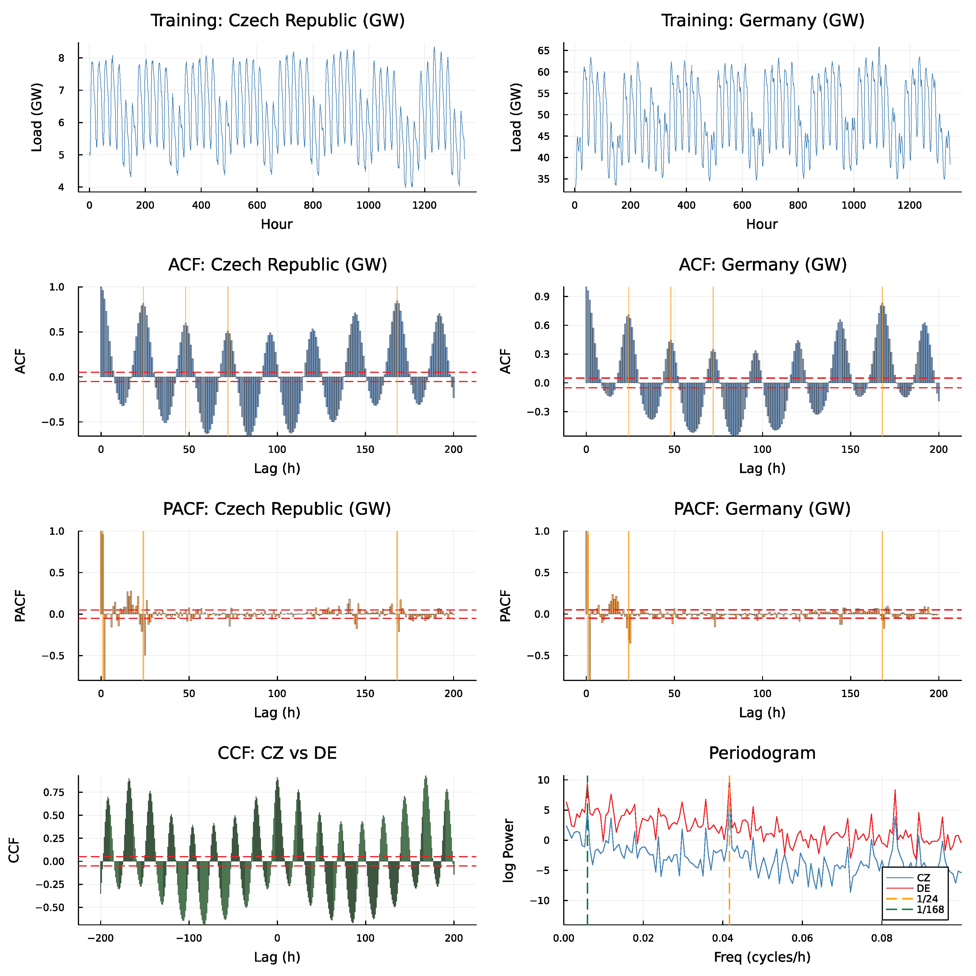
Before fitting any model, we examine the seasonal structure directly from the data. Figure 2 presents the nine-week time series plots together with the sample autocorrelation functions (ACFs) and partial autocorrelation functions (PACFs) as well as the sample cross-correlation functions (CCFs).

The sample ACFs of both series display sharp, persistent spikes at multiples of $s_1=24$ (${\widehat{\rho }}_{\mathrm{CZ}}\left(24\right)=0.818$, ${\widehat{\rho }}_{\mathrm{DE}}\left(24\right)=0.713$) and at $s_2=168$ (${\widehat{\rho }}_{\mathrm{CZ}}\left(168\right)=0.848$, ${\widehat{\rho }}_{\mathrm{DE}}\left(168\right)=0.832$), with no other persistent periodic pattern significant at the 5% level. The sample PACFs cut off sharply after the first lag in each periodicity (${\widehat{\alpha }}_{\mathrm{CZ}}\left(1\right)=0.963$, ${\widehat{\alpha }}_{\mathrm{CZ}}\left(24\right)=-0.253$, ${\widehat{\alpha }}_{\mathrm{CZ}}\left(168\right)=-0.232$), indicating that low-order seasonal AR specifications ($P_1=P_2=1$) are adequate. Periodogram analysis confirms two dominant spectral peaks at $1/24$ and $1/168$ cycles per hour for both series, with no significant power at other frequencies. The CCF in Figure 2 reveals strong contemporaneous and lagged co-movement at the same daily and weekly harmonics, motivating the bivariate DSVAR specification over independent univariate models. Moreover, the Augmented Dickey–Fuller (ADF) test rejects the unit-root null for both series at the 1% level (48 lags, trend specification), confirming stationarity in levels without need for differencing or log transformation.

6.2. DSVAR Selection, Estimation and Residual Diagnostics

Given the confirmed stationarity and the PACF evidence suggesting $P_1=P_2=1$, we fit ${\mathrm{DSVAR}}_2{(p,P_1,P_2)}_{24,168}$ models for $p\in \{1,2\}$, $P_1\in \{1,2\}$, and $P_2\in \{1,2\}$ on the training sample and rank them by AIC, AICc, and BIC computed from the multivariate normal likelihood evaluated at the OLS estimator.

Table 15. Information criteria for DSVAR model order selection (training set, $n_{\mathrm{train}}=1344$).

p	${\mathit{P}}_1$	${\mathit{P}}_2$	AIC	AICc	BIC
2	1	1	$-933.79$	$-929.56$	$-718.64$
1	1	1	$-764.31$	$-762.61$	$-627.37$
2	2	1	$-906.45$	$-895.89$	$-575.64$
1	2	1	$-754.02$	$-749.69$	$-539.92$

reports the results of the highest four DSVAR models.

The ${\mathrm{DSVAR}}_2{(2,1,1)}_{24,168}$ model is selected by BIC (and yields the lowest AIC and AICc), giving $p=2$, $P_1=1$, $P_2=1$, $h=(1+2)(1+1)(1+1)-1=11$, and $kh=22$ regressors per equation. This ordering is consistent with the PACF cutoffs at lags 1, 2, 24, and 168 observed in the exploratory analysis.

The ${\mathrm{DSVAR}}_2{(2,1,1)}_{24,168}$ model is estimated on the first eight weeks ($n_{\mathrm{train}}=1344$ observations), leaving the final week ($n_{\mathrm{test}}=168$) as the hold-out test set. A weakly informative normal-Wishart prior is used: $\mathit{W}=0.01{\mathit{I}}_{22}$, $\mathit{D}=\mathbf{0}$, $a=3$, $\mathbf{\Psi }={\mathit{I}}_2$.

Table 16. Posterior summaries of ${\mathrm{DSVAR}}_2{(2,1,1)}_{24,168}$ coefficient matrices for hourly electricity loads. $\widehat{\mathit{\mu }}$: posterior mean; $\widehat{\mathit{s}}$: posterior SD; $(\widehat{\mathit{L}},\widehat{\mathit{U}})$: 95% credible interval limits.

Param	$\widehat{\mathit{\mu }}$	$\widehat{\mathit{s}}$	$\widehat{\mathit{L}}$	$\widehat{\mathit{U}}$
${\mathit{\varphi }}_1$	$\left[\begin{array}{cc}1.251& 0.468\\ 0.000& 1.159\end{array}\right]$	$\left[\begin{array}{cc}0.035& 0.274\\ 0.004& 0.031\end{array}\right]$	$\left[\begin{array}{cc}1.182& -0.069\\ -0.008& 1.098\end{array}\right]$	$\left[\begin{array}{cc}1.320& 1.005\\ 0.008& 1.220\end{array}\right]$
${\mathit{\varphi }}_2$	$\left[\begin{array}{cc}-0.282& -0.202\\ -0.003& -0.254\end{array}\right]$	$\left[\begin{array}{cc}0.035& 0.277\\ 0.004& 0.031\end{array}\right]$	$\left[\begin{array}{cc}-0.351& -0.745\\ -0.011& -0.315\end{array}\right]$	$\left[\begin{array}{cc}-0.213& 0.341\\ 0.005& -0.193\end{array}\right]$
${\mathbf{\Psi }}_1$	$\left[\begin{array}{cc}0.208& -0.591\\ -0.005& 0.231\end{array}\right]$	$\left[\begin{array}{cc}0.036& 0.282\\ 0.004& 0.031\end{array}\right]$	$\left[\begin{array}{cc}0.137& -1.143\\ -0.013& 0.170\end{array}\right]$	$\left[\begin{array}{cc}0.279& -0.039\\ 0.003& 0.292\end{array}\right]$
${\mathbf{\Gamma }}_1$	$\left[\begin{array}{cc}0.228& 0.445\\ -0.003& 0.224\end{array}\right]$	$\left[\begin{array}{cc}0.057& 0.445\\ 0.006& 0.048\end{array}\right]$	$\left[\begin{array}{cc}0.116& -0.427\\ -0.015& 0.130\end{array}\right]$	$\left[\begin{array}{cc}0.340& 1.317\\ 0.009& 0.318\end{array}\right]$

reports the posterior mean, posterior standard deviation, and 95% credible interval for the four primary coefficient blocks.

Several features of Table 16 are noteworthy. The diagonal of ${\mathit{\varphi }}_1$ (1.251, 1.159) and ${\mathit{\varphi }}_2$ ($-0.282$, $-0.254$) indicate a near-unit-root AR(2) structure in levels that together yield stationary dynamics. The pair $({\varphi }_1=1.251,{\varphi }_2=-0.282)$ implies AR roots of modulus approximately $0.930$ and $0.895$, both inside the unit circle. The daily seasonal block ${\mathbf{\Psi }}_1$ has diagonal entries 0.208 and 0.231, confirming that the 24-h lag is a significant and positive predictor after controlling for the regular AR dynamics. The weekly block ${\mathbf{\Gamma }}_1$ has diagonal entries 0.228 and 0.224, capturing the weekday-versus-weekend load differential at the $s_2=168$ lag. The off-diagonal element ${\widehat{\psi }}_{12}=-0.591$ of ${\mathbf{\Psi }}_1$ is the largest off-diagonal in magnitude and is significant (95% CI $[-1.143,-0.039]$), indicating that a high German load 24 h ago predicts a lower Czech load today after accounting for own-lag effects.

The posterior mean precision and covariance matrices are as follows:

$$\mathbb{E}[\mathit{T}\mid {\mathit{S}}_n]=\left[\begin{array}{cc}202.204& -3.994\\ -3.994& 3.308\end{array}\right],\widehat{\mathbf{\Sigma }}={10}^{-3}\left[\begin{array}{cc}5.066& 6.117\\ 6.117& 309.684\end{array}\right]{\mathrm{GW}}^2.$$

(54)

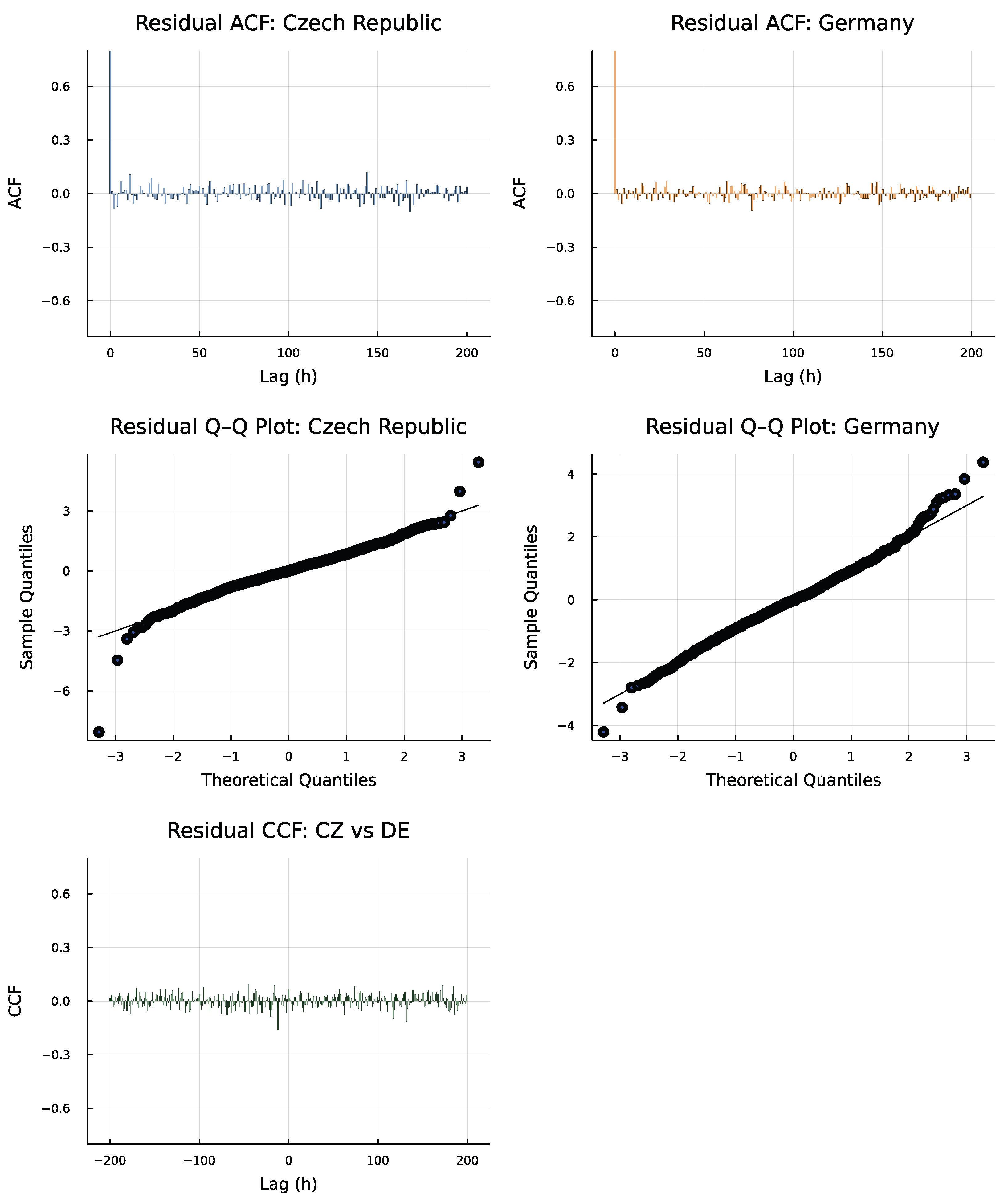
The estimated residual standard deviations are $0.0712$ GW (Czech Republic) and $0.5566$ GW (Germany), both small relative to their respective load scales, confirming excellent in-sample fit. The positive off-diagonal of $\widehat{\mathbf{\Sigma }}$ confirms co-movement of the residuals. In-sample residuals are computed for the fitted ${\mathrm{DSVAR}}_2{(2,1,1)}_{24,168}$ model, and their ACFs, CCF, and Q–Q plot for normality are displayed in Figure 3.

From Figure 3, the residual ACFs are negligible at all lags for both series (maximum $|\widehat{\rho }|\le 0.11$ over lags), confirming that the model captures both the daily and weekly seasonal dynamics completely. In addition, residual cross-correlations at all lags are negligible ($|{\widehat{\rho }}_{12}(\mathsf{\ell })|<0.16$ for $\mathsf{\ell }\ge 1$), indicating that the DSVAR structure adequately captures both contemporaneous and dynamic dependence. All roots of the three estimated determinantal polynomials $|{\widehat{\mathit{\varphi }}}_2\left(z\right)|=0$, $|{\widehat{\mathbf{\Psi }}}_1\left(z^{24}\right)|=0$, $|{\widehat{\mathbf{\Gamma }}}_1\left(z^{168}\right)|=0$ lie strictly outside the complex unit disk (minimum modulus $0.895$), confirming stationarity of the fitted model. Moreover, the Jarque–Bera normality test rejects the Gaussian error assumption at the 1% level for both series. Nevertheless, the Q–Q plots in Figure 3 indicate that the residual distributions remain close to Gaussian, with only mild departures from normality visible in the tails. The non-normality does not invalidate the DSVAR forecasts: the posterior mean $\tilde{\mathit{B}}$ remains the best linear unbiased estimator under the matrix regression model regardless of the error distribution.

6.3. DSVAR Forecasting and Benchmark Comparison

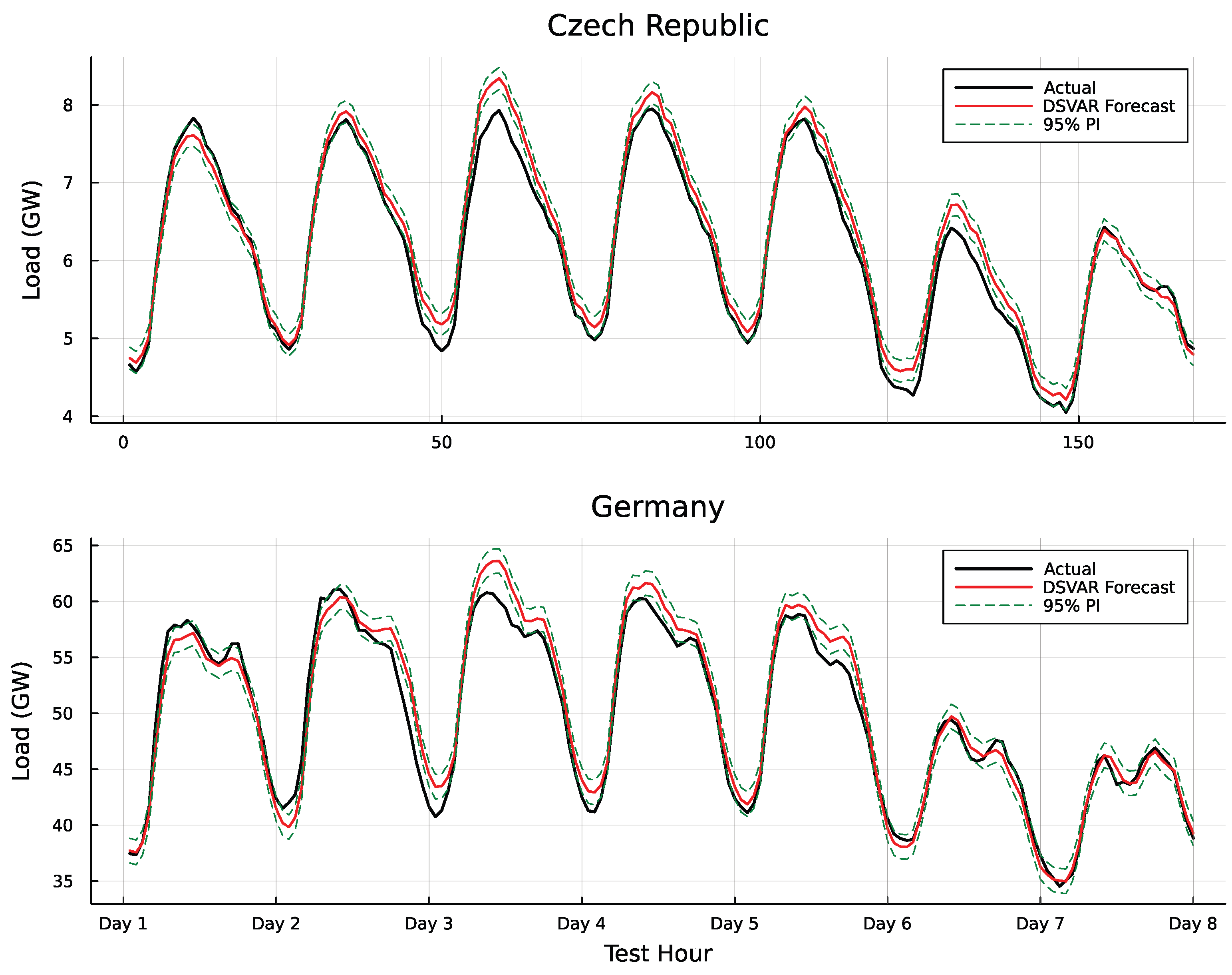
We compute multi-step-ahead forecasts for the 168-h hold-out week using Theorem 2 applied iteratively.

Table 17. Predictive summaries of multi-step-ahead predictions (first five hours) of DSVAR model. $\widehat{\mathit{\mu }}$: predictive mean; $\widehat{\mathit{s}}$: predictive SD; $(\widehat{\mathit{L}},\widehat{\mathit{U}})$: 95% prediction interval.

$\mathit{y}(\mathit{n}+\mathit{r})$	True	$\widehat{\mathit{\mu }}$	$\widehat{\mathit{s}}$	$\widehat{\mathit{L}}$	$\widehat{\mathit{U}}$
$\left[\begin{array}{c}\mathit{y}(n+1)\\ \mathit{y}(n+2)\\ \mathit{y}(n+3)\\ \mathit{y}(n+4)\\ \mathit{y}(n+5)\end{array}\right]$	$\left[\begin{array}{cc}4.660& 37.450\\ 4.570& 37.340\\ 4.700& 38.490\\ 4.940& 41.390\\ 5.810& 48.660\end{array}\right]$	$\left[\begin{array}{cc}4.747& 37.715\\ 4.690& 37.564\\ 4.800& 38.402\\ 5.019& 40.845\\ 5.768& 46.660\end{array}\right]$	$\left[\begin{array}{cc}0.072& 0.562\\ 0.072& 0.562\\ 0.072& 0.561\\ 0.072& 0.565\\ 0.073& 0.574\end{array}\right]$	$\left[\begin{array}{cc}4.606& 36.613\\ 4.549& 36.463\\ 4.659& 37.303\\ 4.878& 39.738\\ 5.624& 45.534\end{array}\right]$	$\left[\begin{array}{cc}4.887& 38.817\\ 4.831& 38.665\\ 4.941& 39.500\\ 5.161& 41.952\\ 5.912& 47.785\end{array}\right]$

reports the predictive summaries for the first five steps, while Figure 4 displays the full 168-h forecast with 95% prediction intervals. The associated RMSE and MAPE statistics are provided for $r=1,168$ in

Table 18. Out-of-sample forecast accuracy of DSVAR model over 168 hold-out hours. RMSE in GW and MAPE in %.

Series	$\mathit{r}=1$		$\mathit{r}=168$
	RMSE	MAPE	RMSE	MAPE
Czech Republic	0.087	1.856	0.206	2.918
Germany	0.265	0.708	1.442	2.280

.

Table 17 and Figure 4 show that the forecasts, including those at extended horizons, exhibit strong concordance with the realized data. The relatively small RMSE and MAPE values in Table 18 further confirm this high level of predictive accuracy. In particular, at the one-step horizon ($r=1$), the model achieves RMSE values of 0.087 GW and 0.265 GW for Czech Republic and Germany, respectively. Relative to the typical load ranges of each system (3.98–8.34 GW for Czech Republic and 32.94–65.84 GW for Germany), these RMSE values confirm that both systems are forecast with comparable relative precision. On a percentage-error basis, Germany attains a lower one-step MAPE (0.71%) than Czech Republic (1.86%), reflecting the smoother aggregate load profile of a larger and more diversified system [4]. Both values fall within the 1–3% range reported in the electricity forecasting literature for competitive short-term methods [2,38], placing the DSVAR results in the upper tier of published benchmarks.

At the 168-step horizon ($r=168$), corresponding to a full weekly cycle, Czech Republic’s MAPE increases only marginally from 1.86% to 2.92%, while its RMSE grows by a factor of 2.37. This exceptional stability is a direct consequence of the double seasonal structure. The second seasonal block ${\mathbf{\Gamma }}_1$ provides an explicit link to the observation exactly one week prior, so the $s_2=168$ lag functions as a near-sufficient predictor at this horizon. By contrast, the data for Germany exhibit relatively more pronounced degradation: MAPE rises from 0.71% to 2.28%, while RMSE grows by a factor of 5.44. Overall, the results confirm that the Bayesian DSVAR framework delivers accurate and well-calibrated forecasts at both horizons, with the double seasonal specification providing the strongest benefit at the longer horizon where the weekly periodicity is most informative.

To assess the practical value of the proposed DSVAR model, we compare its forecasting accuracy against three established benchmark models, and the orders of these benchmarks are selected using the BIC measure. These three benchmarks, together with the order-selection grid searched and the resulting BIC-optimal order, are as follows:

(1)

VAR(p)—a standard non-seasonal VAR model, with p searched over $\{1,\dots ,30\}$. Because hourly data have no explicit seasonal regressor in this model, the search must extend the lag order far enough to span a full day. Thus, the BIC selects $p=27$.

(2)

SVAR${(p,P_1)}_{24}$—a single-seasonal VAR model including only the $s_1=24$ cycle, with $(p,P_1)$ searched over $\{1,\dots ,5\}\times \{1,\dots ,4\}$. The BIC selects $(p,P_1)=(3,3)$.

(3)

SAR${(p,P)}_{24}$—univariate seasonal AR models fitted independently to each series by $(p,P)$ searched over $\{1,\dots ,5\}\times \{1,\dots ,4\}$ per series. The BIC selects $(p,P)=(3,1)$ for Czech Republic and $(p,P)=(2,4)$ for Germany.

Table 19. BIC-optimal orders for the proposed model and all benchmarks (training set, $n_{\mathrm{train}}=1344$).

Model	Search Grid	Selected Order	BIC
${\mathrm{DSVAR}}_2{(p,P_1,P_2)}_{24,168}$	$p,P_1,P_2\in \{1,2\}$	$(2,1,1)$	$-718.64$
${\mathrm{VAR}}_2\left(p\right)$	$p\in \{1,\dots ,30\}$	27	$721.06$
${\mathrm{SVAR}}_2{(p,P_1)}_{24}$	$p\in \{1,\dots ,5\}$, $P_1\in \{1,\dots ,4\}$	$(3,3)$	$500.40$
Univariate ${\mathrm{SAR}}_{\mathrm{CZ}}{(p,P)}_{24}$	$p\in \{1,\dots ,5\}$, $P\in \{1,\dots ,4\}$	$(3,1)$	$-2170.11$
Univariate ${\mathrm{SAR}}_{\mathrm{DE}}{(p,P)}_{24}$	$p\in \{1,\dots ,5\}$, $P\in \{1,\dots ,4\}$	$(2,4)$	$3041.01$

reports the BIC values that determined each selected order alongside the DSVAR result from Table 15 for direct comparison.

The order-selection results in Table 19 are themselves informative. For instance, the non-seasonal VAR requires $p=27$ lags, which is a 27-fold increase over the DSVAR’s regular order $p=2$. Here, daily periodicity is only approximated via unstructured lags, in contrast to the explicit representation provided by the ${\mathbf{\Psi }}_{P_1}\left(B^{s_1}\right)$ operator in the DSVAR. This confirms at the level of model-selection evidence that explicit double seasonal structure is statistically preferred over generic high-order lag inclusion for this dataset. Every benchmark model is then re-estimated at its BIC-selected order on the same 1344-observation training set and evaluated on the same 168-observation hold-out.

Table 20. Out-of-sample forecast accuracy over the 168-h hold-out week, with all models at their BIC-selected order. RMSE is in GW and MAPE in %. Bold indicates the best result in each column.

	Czech Republic				Germany
Method	$\mathit{r}=\mathbf{1}$		$\mathit{r}=\mathbf{168}$		$\mathit{r}=\mathbf{1}$		$\mathit{r}=\mathbf{168}$
	RMSE	MAPE	RMSE	MAPE	RMSE	MAPE	RMSE	MAPE
${\mathrm{DSVAR}}_2{(2,1,1)}_{24,168}$	0.087	1.856	0.206	2.918	0.265	0.708	1.442	2.280
${\mathrm{VAR}}_2\left(27\right)$	0.192	4.111	0.658	9.829	0.481	1.284	4.585	8.071
${\mathrm{SVAR}}_2{(3,3)}_{24}$	0.145	3.115	0.660	10.021	0.325	0.868	5.134	9.320
Univariate ${\mathrm{SAR}}_{24}$	0.235	5.042	0.704	10.729	0.352	0.941	5.256	9.463

reports RMSE (GW) and MAPE (%) at horizons $r=1$ and $r=168$.

The results in Table 20 demonstrate clear and consistent superiority of the proposed Bayesian DSVAR model across both series and both forecast horizons. At the one-step horizon, the DSVAR achieves RMSE reductions of approximately 55% over the standard VAR, 40% over the SVAR, and 63% over the univariate SAR for Czech Republic; comparable gains are observed for the MAPE. The advantage is most pronounced at the 168-step horizon, where the double seasonal structure provides an explicit weekly periodicity link. The DSVAR’s MAPE of 2.92% (Czech Republic) and 2.28% (Germany) compares favorably to the univariate SAR at 10.73% and 9.46%, respectively. The single-seasonal SVAR captures only the daily cycle; therefore, it degrades rapidly at longer horizons when the weekly pattern dominates. These comparisons establish that the DSVAR framework delivers genuine practical improvements and is not merely an incremental theoretical extension.

To confirm that the DSVAR’s accuracy advantage is statistically significant rather than a chance artefact of the single test week, we apply the Diebold and Mariano [39] test (DM test) for equal predictive accuracy. The loss differential is $d_r=e_{\mathrm{DSVAR},r}^2-e_{\mathrm{bench},r}^2$, where $e_r$ is the forecast error at step r and the test statistic is the t-ratio of the sample mean of $d_r$.

Table 21. Diebold–Mariano test for equal predictive accuracy: DSVAR vs. each benchmark. The negative DM statistic indicates that DSVAR has a lower squared error.

Comparison	Czech Republic		Germany
	DM Stat	$\mathit{p}$-Value	DM Stat	$\mathit{p}$-Value
DSVAR vs. ${\mathrm{VAR}}_2\left(27\right)$	$-8.020$	<$0.001$	$-9.418$	<$0.001$
DSVAR vs. ${\mathrm{SVAR}}_2{(3,3)}_{24}$	$-8.221$	<$0.001$	$-12.854$	<$0.001$
DSVAR vs. Univariate ${\mathrm{SAR}}_{24}$	$-8.139$	<$0.001$	$-12.178$	<$0.001$

reports the DM statistics and p-values for DSVAR against each benchmark over the full 168-step horizon. The DSVAR significantly outperforms all three benchmarks for both series at the 0.1% level, confirming that the accuracy gains in Table 20 are not sampling variability.

7. Conclusions

This paper introduces and analyzes the DSVAR model, a multivariate time series framework designed for processes that simultaneously exhibit two seasonal periodicities. The model is defined through a multiplicative triple autoregressive operator, complete expansion of which yields seven structurally interpretable groups of regressors. The core theoretical contributions are exact Bayesian distributional results. Under a conjugate normal-Wishart prior, the marginal posterior of the coefficient matrix is a closed-form matrix-t distribution and that of the precision matrix a Wishart distribution. The one-step-ahead predictive distribution is an exact multivariate-t with an explicit scale matrix and degrees of freedom. Parallel results under Jeffreys’ vague prior are derived, and the pure autoregressive structure ensures that the predictive regressor vector is exact. Monte Carlo simulations confirm the accuracy of the proposed Bayesian estimation and forecasting of the DSVAR models, and a real application to hourly electricity loads in Czech Republic and Germany shows that the DSVAR models provide highly accurate forecasts that outperform standard VAR, seasonal VAR, and univariate seasonal AR benchmarks at both short and long forecast horizons.

The proposed framework has some important limitations and assumptions that should be acknowledged. First, the Gaussian error assumption may not hold for all high-frequency data, particularly when heavy-tailed innovations or outliers are present; extensions to Student-t error distributions represent a natural direction for future work. Second, the model assumes fixed and known seasonal periods $s_1$ and $s_2$; when these are uncertain, a model selection step or fully Bayesian treatment of the periods would be needed. Third, in large-dimensional systems (large k), the $kh\times kh$ matrix $\mathit{A}$ requires inversion, which has computational cost $O\left(k^3{h}^3\right)$. While this remains feasible for small k and low DSVAR orders, it requires structured approximations (e.g., Kronecker factorization or sparse precision matrices) for very large k. Finally, the empirical application used nine weeks of data; a longer sample covering more seasonal cycles and holiday effects would provide a more comprehensive out-of-sample evaluation, which we leave for future work.

Future work could include time-varying coefficient versions of the DSVAR model that would accommodate structural changes in seasonal patterns, building on the large time-varying parameter VAR literature. A systematic comparison with non-parametric and machine learning-based multiseasonal forecasting approaches would further delineate the conditions under which the interpretability and analytical tractability of the DSVAR framework provide a practical advantage.

References

1. Amin, A.A. Bayesian analysis of double seasonal autoregressive models. Sankhya B 2020, 82, 328–352. [Google Scholar]
2. Taylor, J.W. Short-Term Electricity Demand Forecasting Using Double Seasonal Exponential Smoothing. J. Oper. Res. Soc. 2003, 54, 799–805. [Google Scholar] [CrossRef] [Scilit]
3. Taylor, J.W. An Evaluation of Methods for Very Short-Term Load Forecasting Using Minute-by-Minute British Data. Int. J. Forecast. 2008, 24, 645–658. [Google Scholar] [CrossRef] [Scilit]
4. Weron, R. Electricity Price Forecasting: A Review of the State-of-the-Art with a Look into the Future. Int. J. Forecast. 2014, 30, 1030–1081. [Google Scholar] [CrossRef] [Scilit]
5. Amin, A.A. Full Bayesian analysis of double seasonal autoregressive models with real applications. J. Appl. Stat. 2024, 51, 1524–1544. [Google Scholar] [PubMed]
6. Cottet, R.; Smith, M. Bayesian Modeling and Forecasting of Intraday Electricity Load. J. Am. Stat. Assoc. 2003, 98, 839–849. [Google Scholar] [CrossRef] [Scilit]
7. Gianfreda, A.; Grossi, L. Forecasting Italian Electricity Zonal Prices with Exogenous Variables. Energy Econ. 2012, 34, 2228–2239. [Google Scholar] [CrossRef] [Scilit]
8. Taylor, J.W. Triple Seasonal Methods for Short-Term Electricity Demand Forecasting. Eur. J. Oper. Res. 2010, 204, 139–152. [Google Scholar] [CrossRef] [Scilit]
9. Wichard, J.D. Forecasting the NN5 time series with hybrid models. Int. J. Forecast. 2011, 27, 700–707. [Google Scholar] [CrossRef] [Scilit]
10. Amin, A.A.; Ismail, M.A. Gibbs sampling for double seasonal autoregressive models. Commun. Stat. Appl. Methods 2015, 22, 557–573. [Google Scholar] [CrossRef] [Scilit]
11. Amin, A.A. Bayesian inference for double seasonal moving average models: A gibbs sampling approach. Pak. J. Stat. Oper. Res. 2017, 13, 483–499. [Google Scholar] [CrossRef] [Scilit]
12. Amin, A.A. Bayesian inference for double SARMA models. Commun. Stat.-Theory Methods 2018, 47, 5333–5345. [Google Scholar]
13. Sims, C.A. Macroeconomics and Reality. Econometrica 1980, 48, 1–48. [Google Scholar] [CrossRef] [Scilit]
14. Lütkepohl, H. New Introduction to Multiple Time Series Analysis; Springer: Berlin/Heidelberg, Germany, 2006. [Google Scholar] [CrossRef]
15. Litterman, R.B. Forecasting with Bayesian Vector Autoregressions—Five Years of Experience. J. Bus. Econ. Stat. 1986, 4, 25–38. [Google Scholar] [CrossRef] [Scilit]
16. Doan, T.; Litterman, R.; Sims, C. Forecasting and Conditional Projection Using Realistic Prior Distributions. Econom. Rev. 1984, 3, 1–100. [Google Scholar] [CrossRef] [Scilit]
17. Kadiyala, K.R.; Karlsson, S. Numerical Methods for Estimation and Inference in Bayesian VAR-Models. J. Appl. Econom. 1997, 12, 99–132. [Google Scholar] [CrossRef]
18. Bańbura, M.; Giannone, D.; Reichlin, L. Large Bayesian Vector Auto Regressions. J. Appl. Econom. 2010, 25, 71–92. [Google Scholar] [CrossRef] [Scilit]
19. Giannone, D.; Lenza, M.; Primiceri, G.E. Prior Selection for Vector Autoregressions. Rev. Econ. Stat. 2015, 97, 436–451. [Google Scholar] [CrossRef] [Scilit]
20. Shaarawy, S.M.; Ali, S.S. Bayesian Identification of Seasonal Multivariate Autoregressive Processes. Commun. Stat.-Theory Methods 2015, 44, 823–836. [Google Scholar] [CrossRef] [Scilit]
21. Shaarawy, S.M.; Ali, S.S. Bayesian Identification of Multivariate Autoregressive Processes. Commun. Stat.-Theory Methods 2008, 37, 791–802. [Google Scholar] [CrossRef] [Scilit]
22. Shaarawy, S.M.; Ali, S.S. Bayesian Identification of Seasonal Autoregressive Models. Commun. Stat.-Theory Methods 2003, 32, 1067–1084. [Google Scholar] [CrossRef] [Scilit]
23. Shaarawy, S.M. Bayesian Modeling and Forecasting of Vector Autoregressive Moving Average Processes. Commun. Stat.-Theory Methods 2021, 52, 3795–3815. [Google Scholar] [CrossRef] [Scilit]
24. Shaarawy, S.; Ali, S.; Soliman, E. A Bayesian Procedure to Identify the Orders of Vector Moving Average Processes with Seasonality. Egypt. Stat. J. 2020, 64, 1–20. [Google Scholar] [CrossRef] [Scilit]
25. Albassam, M.; Soliman, E.E.; Ali, S.S. An effectiveness study of the Bayesian inference with multivariate autoregressive moving average processes. Commun. Stat.-Simul. Comput. 2023, 52, 4773–4788. [Google Scholar] [CrossRef] [Scilit]
26. Shaarawy, S.M.; Ali, S.S.; Salam, E.E.A. Bayesian Identification of Seasonal Vector ARMA Processes. Egypt. Stat. J. 2024, 68, 129–145. [Google Scholar] [CrossRef] [Scilit]
27. Box, G.E.P.; Jenkins, G.M. Time Series Analysis: Forecasting and Control; Holden-Day: San Francisco, CA, USA, 1970. [Google Scholar]
28. Box, G.E.P.; Tiao, G.C. Bayesian Inference in Statistical Analysis; Addison-Wesley: Reading, MA, USA, 1973. [Google Scholar]
29. Shaarawy, S.M. Bayesian Inferences and Forecasts with Multiple ARMA Models. Commun. Stat.-Simul. Comput. 1989, 18, 1481–1509. [Google Scholar] [CrossRef] [Scilit]
30. Zellner, A. An Introduction to Bayesian Inference in Econometrics; John Wiley & Sons: New York, NY, USA, 1971. [Google Scholar]
31. Broemeling, L.D.; Shaarawy, S.M. Time Series: A Bayesian Analysis in the Time Domain. In Bayesian Analysis of Time Series and Dynamic Models; Spall, J.C., Ed.; Marcel Dekker: New York, NY, USA, 1988; pp. 1–22. [Google Scholar]
32. Sims, C.A.; Zha, T. Bayesian Methods for Dynamic Multivariate Models. Int. Econ. Rev. 1998, 39, 949–968. [Google Scholar] [CrossRef] [Scilit]
33. Chatfield, C. Calculating Interval Forecasts. J. Bus. Econ. Stat. 1993, 11, 121–135. [Google Scholar] [CrossRef] [Scilit]
34. West, M.; Harrison, J.; Migon, H.S. Dynamic Generalised Linear Models and Bayesian Forecasting. J. Am. Stat. Assoc. 1985, 80, 73–83. [Google Scholar] [CrossRef]
35. Tiao, G.C.; Zellner, A. On the Bayesian Estimation of Multivariate Regression. J. R. Stat. Soc. Ser. B 1964, 26, 277–285. [Google Scholar] [CrossRef] [Scilit]
36. Rossi, P.E.; Allenby, G.M.; McCulloch, R. Bayesian Statistics and Marketing; John Wiley & Sons: Chichester, UK, 2005. [Google Scholar] [CrossRef] [Scilit]
37. Zellner, A. Models, Prior Information, and Bayesian Analysis. J. Econom. 1996, 75, 51–68. [Google Scholar] [CrossRef] [Scilit]
38. Makridakis, S.; Hibon, M. The M3-Competition: Results, Conclusions and Implications. Int. J. Forecast. 2000, 16, 451–476. [Google Scholar] [CrossRef] [Scilit]
39. Diebold, F.X.; Mariano, R.S. Comparing Predictive Accuracy. J. Bus. Econ. Stat. 1995, 13, 253–263. [Google Scholar] [CrossRef] [Scilit]
Figure 1. Representative realizations of the simulated DSVAR models for n = 200 time points.
Mathematics 14 02870 g001
Figure 2. Time plots, ACFs, PACFs, and CCF of hourly electricity loads in Czech Republic and Germany. Orange vertical lines in the ACFs and PACFs mark lags 24, 48, 96, and 168.
Mathematics 14 02870 g002
Figure 3. Residual ACFs, CCF, and Q–Q plot for normality of the fitted DSVAR 2 ( 2 , 1 , 1 ) 24 , 168 model applied to hourly electricity loads in Czech Republic and Germany.
Mathematics 14 02870 g003
Figure 4. Bayesian forecasts of electricity load in Czech Republic and Germany: actual values (black), posterior predictive mean (red), and 95% prediction interval (green shading) over the 168-h test week.
Mathematics 14 02870 g004