Demand-Oriented Post-Disaster Repair Scheduling for a Power-Grid-Building System

Abstract

Post-disaster repair priorities can change when building demand and available supply recover at different rates. This study models a power-grid-building system, defines demand loss as cumulative unmet demand divided by cumulative demand, and uses a genetic algorithm (GA) with deterministic feasibility rules to select repair task order and repair mode. The two GA searches used the same settings, 20 runs for each objective, and 36,200 schedules evaluated per run. In the baseline case, the lowest demand loss found was 0.3925 for the demand-targeted search and 0.3995 for the supply-targeted search. The demand-targeted result was 1.7464% lower and reduced cumulative unmet demand by 238 kW-day. Across the same 20 random seeds, the demand-targeted search produced lower demand loss in 16 runs and the supply-targeted search produced lower demand loss in four runs. In a separate comparison with different computational effort, the demand-targeted GA result had 20.3% lower demand loss than one deterministic greedy schedule. Additional five-run analyses show that the observed results depend on GA settings, crew availability, repair duration, and demand timing. The findings apply to the tested deterministic case study and support demand-aware repair scheduling when demand and supply recover at different rates.

1. Introduction

Electricity service supports essential residential, commercial, and public functions, while disaster-related outages can impose uneven and prolonged service burdens across affected communities [1,2,3,4,5]. Recovery planning, therefore, requires more than tracking the return of aggregate generation or distribution capacity: it also requires attention to when and where electricity demand re-emerges as buildings and community activities recover. In this study, a power-grid-building system denotes a distribution network coupled to the building demand clusters served by its supply nodes. The scope is limited to repair scheduling within this coupled abstraction; it does not include a transportation network, repair routing, AC or DC power flow, network reconfiguration, or real-time operational control.

The reviewed literature contains three related groups. Repair scheduling studies optimize component order, crews, reconfiguration, or load restoration [6,7,8]; later work also considers blackout repair tasks and switch uncertainty [9,10]. Demand-side studies represent response, flexible load, or observed changes in electricity use [11,12,13,14], while empirical and Bayesian studies show that activity and recovery trajectories can vary over time [15,16,17]. Integrated recovery frameworks represent interacting infrastructure or changing supply and demand [18,19,20,21,22]. These groups address important parts of the problem, but the reviewed studies do not combine a time-varying building demand profile with the discrete repair order and crew-mode decisions used here.

A repair schedule that restores the most supply may not minimize unmet demand when demand recovers unevenly across nodes and time. We, therefore, evaluate schedules by system-wide demand loss: cumulative unmet demand divided by cumulative demand over the 14-day objective horizon. This study makes three contributions:

• A power-grid-building abstraction links 33 supply nodes to 33 corresponding demand nodes and evaluates time-varying service deficits under fixed topology and dispatch assumptions.
• A two-part GA represents repair task order and repair mode, while fixed decoding rules assign feasible non-preemptive start times under the crew limit.
• The numerical evaluation compares demand-targeted and supply-targeted GA searches using 20 independent runs with preset random seeds, examines GA parameter sensitivity, compares the GA result with a deterministic constructive greedy schedule, and evaluates one-factor sensitivity to crew availability, repair duration, and demand recovery timing.

2. Literature Review

2.1. Resilience Metrics and Recovery Trajectories

The resilience triangle concept describes loss through the depth and duration of reduced system performance [23,24]. Power system studies use related metrics for outage consequences, service restoration, and available capacity, but the units and normalization depend on the decision purpose [25,26,27,28,29]. Demand–supply frameworks instead track unsatisfied service as supply and demand change [18,19]. Empirical electricity use and human activity studies show that post-event demand need not return uniformly [12,15,16], and Bayesian recovery models provide a separate route for estimating uncertain recovery trajectories [17]. The present study does not calibrate those models; it uses their broader motivation to define a transparent scheduling objective based on cumulative unmet demand.

2.2. Repair Scheduling Without Time-Varying Demand Recovery

Arif et al. jointly schedule repair, reconfiguration, and distributed generation dispatch [6]. Tan et al. study component repair with one or multiple crews [7], and Yan et al. include sequence-dependent repair periods and load accommodation [8]. Pang et al. formulate emergency repair task scheduling for large-scale blackouts [9], while Zhu et al. study repair crew dispatch under switch uncertainty [10]. Canbilen Sütiçen et al. consider reinforcement and repair in interdependent networks under disaster uncertainty [22]. These studies include broader crew, network, or uncertainty decisions than our case study. However, none of the formulations reviewed here uses a recovering building demand profile to choose repair order and crew mode.

2.3. Demand Recovery Without Repair Sequence Decisions

Demand-side and operational studies address a different problem. Song et al. model demand response from thermostatically controlled loads [11]; Li et al. combine demand-side management with topology adaptation under windstorms [13]; and Jalilpoor et al. and Hadi et al. use demand flexibility in multi-energy or microgrid operation [14,30]. Stochastic electric vehicle integration and risk-based resilience planning broaden the uncertainty and planning scope [31,32], while integrated energy planning includes storage, sharing, and demand-side management [33]. These studies show that flexible or uncertain demand can affect operation, but they do not choose the repair task order and crew mode studied here.

2.4. Integrated and Data-Driven Recovery Models

Sun et al. simulate interactions between electric power supply and community recovery after earthquakes [18], and Didier et al. quantify unsatisfied demand through a compositional demand–supply framework [19]. Jiang et al. coordinate distribution, energy, and transportation recovery [20], whereas Zhang et al. study multi-energy load restoration [21]. Other work uses graph-neural network surrogates for resilience-oriented network design [34] or reinforcement learning for infrastructure recovery [35,36]. Hazard-specific assessment under high-power microwave disturbance addresses another part of resilience analysis [37]. These methods widen the modeled system or solution approach, but they do not directly answer the narrower scheduling question examined here.

2.5. Research Gap and Scope

The reviewed studies leave a specific scheduling gap. Time-varying demand and unmet service metrics already exist [15,16,17,18,19], and detailed repair scheduling already exists as well [6,7,8,9,10,22]. This study combines these elements by using a recovering building demand profile to evaluate discrete repair order and crew-mode decisions under the stated one-to-one service rule. It does not claim that demand recovery, resilience metrics, or repair scheduling is new on its own. The model also excludes transportation, routing, switching, repair cost, and probabilistic damage. Probabilistic repair time studies in other infrastructure classes suggest a future extension but do not calibrate the electrical duration matrix used here [38].

2.6. Choice of Solution Method

The solution method must match the decision representation. Mixed-integer formulations can provide bounds for a specified model, although their performance depends on the formulation and instance [6,7]. Particle swarm optimization and differential evolution have also been applied to restoration problems [39,40]. The GA used here works directly with a task permutation and a discrete repair-mode vector, and then applies fixed decoding rules to produce a feasible schedule [41]. This representation is the reason for selecting the GA in this study. Related GA applications include resilience-oriented storage siting [42].

Table 1. Qualitative comparison of representative resilience and repair scheduling studies.

Ref.	Key Method	Demand Model	Time- Varying Demand Recovery	Resilience Metric	Demand-Oriented Objective	Repair Sequence Optimized	Resource Constraints Considered
Arif et al. [6]	MIP	Static	×	Restored load	×	√	√
Tan et al. [7]	LP-based heuristic	Static	×	Interruption duration	×	√	×
Yan et al. [8]	Two-stage heuristic	Static	×	Load capability/Makespan	×	√	×
Sun et al. [18]	Agent- based (rules)	Supply–demand gap	√	Demand-supply ratio	×	×	×
Didier et al. [19]	Compositional framework	Community demand	×	Resilience configurations	×	×	×
Song et al. [11]	Two-stage DR	Flexible loads	×	Supply adequacy	×	×	×
Li et al. [13]	DSM with real-time pricing	Price-responsive	×	Load reduction	×	×	×
Jalilpoor et al. [14]	Two-stage LP	Flexible loads	×	Supply adequacy	×	×	√
Otsuka [12]	Empirical analysis	Empirical demand behavior	×	Demand elasticity	×	×	×
This work	MIP + GA	Time-varying demand recovery	√	Power deficit (demand-oriented)	√	√	√

summarizes the most relevant distinctions. Each citation is tied to a specific modeling or methodological point; numerical results are not ranked across studies because the networks, objectives, assumptions, and computational effort differ.

3. Methodology

3.1. Problem Definition and Modeling Workflow

The model represents a damaged supply network in which each supply node serves one paired building demand node. Each damaged supply node becomes a repair task. A candidate solution specifies the task order and a repair mode, meaning the number of crews assigned and the corresponding repair duration. Fixed decoding rules then assign the earliest feasible non-preemptive start time under the total crew limit. For each daily interval, the resulting schedule determines local capacity, network connectivity, available supply, served demand, and unmet demand. Section 4 provides the network size, initial damage, and other case study values.

3.2. Demand Service, Objectives, and Time Intervals

Let A_i(t) denote available power and D_i(t) paired demand for node i during objective interval t. Served demand is their minimum, and power deficit is the nonnegative difference between demand and available power. Multiplying power by the interval duration gives energy-equivalent service quantities in kW-day. Summing the deficit over all node pairs and objective intervals gives cumulative unmet demand; summing demand over the same support gives cumulative system demand. Their ratio is the dimensionless demand loss.

Both objectives are evaluated over exactly 14 daily intervals: [0,1), [1,2), …, [13,14), indexed by t = 0, …, 13. The demand profile also reports the state at day 14, giving 15 reporting boundaries from day 0 to day 14. Day 14 is reported but is not a 15th objective interval. The supply loss calculation uses the same 14 interval states.

3.2.1. Time and Index Definitions

Let $𝒩$ = {1, …, n} be the set of paired supply and demand nodes, $𝒥$ ⊂ $𝒩$ the set of damaged supply nodes and their repair tasks, and $𝒯$ = {0, …, 13} the 14 one-day objective intervals [t, t + 1). Thus, i ∈ $𝒩$, j ∈ $𝒥$, and t ∈ $𝒯$. Day 14 is the terminal reporting boundary only, and Δt = 1 day.

3.2.2. Served Demand and Power Deficit

$$q_i(t)=\mathrm{m}\mathrm{i}\mathrm{n}\{A_i(t),D_i(t)\},u_i(t)=\mathrm{m}\mathrm{a}\mathrm{x}\{D_i(t)-A_i(t),0\}.$$

(1)

A_i(t) is available supply at supply node i (kW); D_i(t) is the paired building demand (kW); q_i(t) is served demand (kW); and u_i(t) is unmet power demand or power deficit (kW). Unused supply is not reassigned between node pairs.

3.2.3. Cumulative Unmet Demand and Demand Loss

$$\mathrm{C}\mathrm{U}\mathrm{D}={\sum }_{t\in \mathcal{T}}{\sum }_{i\in \mathcal{N}}{u}_i(t)\Delta \mathrm{t}[\mathrm{kW}-\mathrm{day}].$$

(2)

$$C_D={\sum }_{t\in \mathcal{T}}{\sum }_{i\in \mathcal{N}}{D}_i(t)\Delta \mathrm{t}[\mathrm{kW}-\mathrm{day}].$$

(3)

$$R_D={\displaystyle \frac{CUD}{C_D}}, C_D>0.$$

(4)

A zero-demand node interval contributes zero to both sums; no nodewise division is used. C_D is cumulative system demand and, when C_D > 0, R_D ∈ [0, 1] is the dimensionless demand loss minimized by the demand-targeted GA. If C_D = 0, the evaluation is rejected.

3.2.4. Supply Loss and Average Available Supply

Let C_i be the pre-disaster nameplate supply capacity of node i (kW), and let N_T = 14 be the number of objective intervals.

$$R_S={\displaystyle \frac{{\sum }_{t\in \mathcal{T}}{\sum }_{i\in \mathcal{N}}[C_i-A_i(t\left)\right]\Delta t}{N_T{\sum }_{i\in \mathcal{N}}{C}_i\Delta t}}, 0\le R_S\le 1.$$

(5)

$$\overline{A}={\displaystyle \frac{1}{\left|\mathcal{T}\right|}}{\sum }_{t\in \mathcal{T}}{\sum }_{i\in \mathcal{N}}{A}_i(t)=(1-R_S){\sum }_{i\in \mathcal{N}}{C}_i\left[\mathrm{kW}\right].$$

(6)

R_S is the dimensionless supply loss and Ā is average daily available supply over the 14 objective intervals.

3.2.5. Availability and Traversability State

Let κ_i ∈ {1, 0.75, 0.5, 0.25, 0} be the specified DS1–DS5 functionality multiplier and let z_i(t) indicate root connectivity through traversable nodes in the static radial topology. For a damaged node i ∈ $𝒥$, s_i and c_i denote its decoded repair start and completion times. The local capacity state is as follows.

$$L_i(t)=\{\begin{array}{cc}0& i\in \mathcal{J},s_i\le t<c_i\\ C_i& i\in \mathcal{J},t\ge c_i\\ {\kappa }_i{C}_i& \mathrm{otherwise}\end{array}.$$

(7)

Under the adopted node traversability rule, unrepaired DS1–DS4 nodes are traversable, unrepaired DS5 nodes are not traversable, active repairs are not traversable, and completed repairs are traversable. Available supply is as follows.

$$A_i(t)=z_i(t)L_i(t).$$

(8)

Normally open ties remain open, and unused capacity is not redistributed.

3.2.6. Repair Timing and Modes

A chromosome comprises a task permutation π and one repair mode m_j ∈ {1,2,3} for each task. The decoder assigns integer start time s_j (day), duration τ_j,mj (day), and crew demand r_j,mj (crews). Completion time is as follows.

$$c_j=s_j+{\tau }_{j,m_j}.$$

(9)

Task j occupies crews on the half-open interval [s_j, c_j), which is active when s_j ≤ t < c_j and is complete when t ≥ c_j. Repairs are non-preemptive. Completion after the reporting horizon is allowed and durations are not truncated.

3.2.7. Crew Capacity

$${\sum }_{j\in \mathcal{J}}{r}_{j,m_j}1\{s_j\le t<c_j\}\le R, t\in \{0,\dots ,{max}_{j\in \mathcal{J}}{c}_j-1\}.$$

(10)

R is the total number of available crews and r_jm_j ∈ {1, 2, 3}. The decoder assigns the earliest feasible integer start in permutation order while enforcing the total crew limit and the fixed node traversability rule. The permutation is a priority list, not a finish-to-start precedence relation; there are no predecessor or successor sets. The baseline value R = 6 is specified with the case study inputs in Section 4.

3.2.8. Number of Evaluated Schedules

$$N_{\mathrm{eval}}=P+(P-E)G.$$

(11)

P is the population size, E is the number of unchanged elites retained without re-evaluation in each generation, G is the number of offspring generations, and Neval is the number of schedule evaluations. For P = 200, E = 20, and G = 200, each run evaluates 36,200 schedules.

3.3. Component States, Topology, and Dispatch

Initial supply node functionality is represented by the case study multipliers DS1 = 1.00, DS2 = 0.75, DS3 = 0.50, DS4 = 0.25, and DS5 = 0. Before repair, DS1–DS4 nodes are traversable and retain their corresponding local capacity; DS5 nodes block transit. A node under active repair has zero local capacity and is not traversable. After repair, it becomes DS1, regains full local capacity, and is traversable. Reachability is recomputed from root node 1 during every objective interval, and the root follows the same rule.

A non-preemptive repair starting at integer day sj with duration τj occupies the half-open interval [sj, sj + τj). It consumes crews and blocks the node for exactly those daily intervals; crews are released at completion before another repair may start. The baseline has six crews, with at most three assigned to one task. The duration matrix, crew availability, damage functionality multipliers, one-to-one mapping, static dispatch, and baseline demand profile introduced in Section 4 are fixed case study inputs or modelling rules rather than universally calibrated values.

3.4. Scheduling Formulation and Chromosome

The implemented search represents each solution by a permutation of the |$𝒥$| damaged repair tasks and a |$𝒥$|-entry repair-mode vector. Each mode assigns one, two, or three crews and the corresponding repair duration. The decoder appends undamaged DS1 nodes with mode zero, processes damaged tasks in permutation order, and assigns the earliest feasible integer start time under the total crew limit. Start times are decoder outputs rather than chromosome genes.

The permutation is a priority list rather than a finish-to-start precedence relation. Repairs may overlap when crews are available, and a later task need not wait for every earlier task to finish. The model inputs and decoder contain no predecessor or successor sets. Network connectivity affects interval supply through reachability, not through a repair precedence constraint.

3.5. Genetic Algorithm and Schedule Evaluation Accounting

The GA minimizes the selected loss directly. Parent selection uses independent binary tournaments of size two. Order-crossover-one (OX1) operates on the task permutation, and complementary uniform crossover operates on the mode vector. Mutation consists of a two-position swap in the permutation and a forced change in one repair-mode gene. Permutation and mode crossover have independent pair-level probabilities, and the two mutation operators have independent offspring-level probabilities. Full generational replacement retains E elites without re-evaluation and evaluates P-E new offspring; valid duplicates are retained.

The main GA setting uses P = 200, E = 20, G = 200, permutation/mode crossover probabilities 0.9/0.9, and permutation/mode mutation probabilities 0.1/0.1. Generation 0 contains the initial P schedule evaluations. A run with G completed generations, therefore, uses P + (P − E)G evaluations, giving 36,200 evaluations at the main setting. The search stops after G = 200; there is no stagnation rule. Candidates are ranked first by the objective being minimized, then by task order, mode vector, and a fixed deterministic row order. The other loss is not used for selection or tie breaking.

These operators match the two-part chromosome, and every candidate passes through the same feasibility decoder. The GA returns the best schedule found within the specified runs; it does not prove global optimality.

4. Case Study

4.1. Network Configuration and Initial Damage

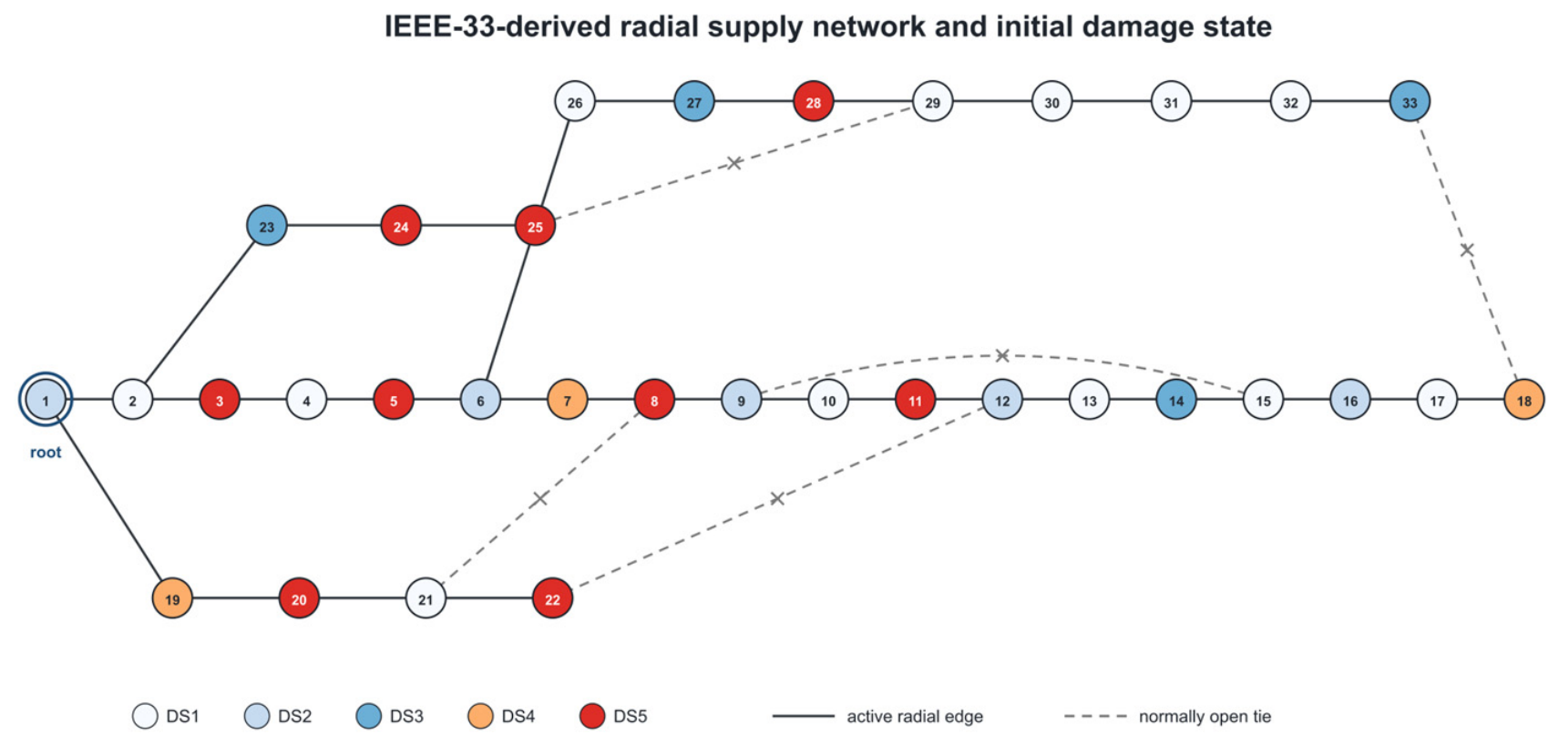
The case study uses a radial network derived from the IEEE 33-bus feeder [43]. It contains 33 supply nodes and 33 one-to-one demand nodes. Node 1 is the root; the 32 radial edges are active and the five tie lines remain normally open. Twenty-one supply nodes begin in damage states DS2–DS5 and, therefore, form the repair task set; the remaining 12 DS1 nodes are undamaged non-tasks. The baseline has six crews, with at most three crews assigned to one task. Figure 1 shows the topology and initial damage state, and

Table 2. Case study configuration and modeling boundary.

Case Study Element	Case Study Setting
Supply network	IEEE-33-derived radial topology; 33 supply nodes; node 1 root
Demand representation	33 one-to-one paired demand nodes; unused capacity is not redistributed
Active/open edges	32 active radial edges; 5 normally open tie lines
Initial damage	21 damaged DS2–DS5 repair tasks; 12 undamaged DS1 non-tasks
Repair resources	6 crews in baseline; maximum 3 crews per task
Objective time support	14 daily intervals [0, 1), …, [13, 14); day 14 reporting only
Repair state rule	Repair occupies [s, s + τ); active node has zero local capacity
Topology/dispatch	Static topology; reachability-based supply; one-to-one dispatch
Excluded operations	No routing, switching, power flow, repair cost, or spare part model

These are fixed case study assumptions and computational settings.

summarizes the fixed case study configuration.

4.2. Demand Profiles and Controlled Scenarios

S0 is an illustrative baseline demand profile constructed for this case study, not a measured post-disaster record. S1–S3 redistribute demand across nodes and time to test whether the comparison changes under different demand patterns. They are controlled deterministic scenarios, not probability samples or observations from different earthquakes. Practical use would require calibration and regular updates from measured and forecast data.

Table A1. (a) S0 baseline demand profile, days 0–7 (kW). (b) S0 baseline demand profile, days 8–14 (kW).

(a)
Node	Day 0	Day 1	Day 2	Day 3	Day 4	Day 5	Day 6	Day 7
1	46	46	46	58	58	69	69	69
2	32	32	33	33	33	33	37	45
3	62	62	62	62	73	73	73	73
4	77	77	78	78	78	78	78	78
5	73	73	73	73	89	89	89	98
6	82	82	82	82	82	82	82	82
7	112	112	112	112	112	112	112	112
8	7	7	7	7	7	7	7	7
9	16	16	16	18	20	20	22	23
10	162	162	162	162	162	200	200	200
11	168	168	168	168	168	200	200	200
12	19	19	19	19	19	19	19	19
13	13	17	17	18	18	21	21	21
14	9	21	21	21	21	25	28	28
15	49	57	57	57	57	57	57	57
16	43	52	52	53	53	53	53	53
17	65	65	65	65	76	79	79	79
18	16	20	20	23	23	24	24	29
19	4	16	16	16	17	17	20	20
20	29	29	29	33	37	37	37	37
21	90	90	90	90	90	90	90	90
22	17	17	17	17	17	21	21	21
23	41	41	41	52	60	60	60	60
24	34	34	34	39	45	45	45	50
25	114	114	114	114	114	114	114	114
26	88	102	102	102	104	104	112	137
27	75	99	99	99	103	105	105	105
28	82	107	107	107	107	107	107	124
29	12	12	12	14	14	14	14	14
30	79	84	84	84	84	84	84	84
31	290	290	290	290	290	290	336	336
32	0	0	0	0	0	0	0	0
33	41	41	41	41	41	41	41	41
(b)
Node		Day 8	Day 9	Day 10	Day 11	Day 12	Day 13	Day 14
1		72	72	72	72	73	73	73
2		48	58	58	58	58	68	68
3		73	73	73	73	73	73	73
4		79	89	89	89	89	89	89
5		98	98	98	98	98	98	98
6		82	82	82	82	82	82	82
7		112	112	112	112	112	112	112
8		8	9	9	9	9	9	9
9		23	23	29	30	30	30	30
10		200	200	200	200	200	200	200
11		200	200	200	200	200	200	200
12		22	22	22	22	22	22	22
13		25	25	25	25	32	36	37
14		28	28	28	28	28	28	35
15		57	57	57	57	57	57	57
16		53	53	53	53	60	60	60
17		79	79	79	79	79	79	79
18		30	30	35	35	35	35	35
19		20	20	20	20	20	20	20
20		43	43	43	49	49	49	49
21		90	90	90	90	90	90	90
22		21	21	21	26	26	26	32
23		60	60	60	60	60	60	60
24		50	50	51	51	51	60	60
25		114	114	114	114	114	114	114
26		137	160	160	182	182	182	182
27		105	105	105	127	130	149	149
28		124	124	160	160	160	160	160
29		14	15	15	15	15	15	15
30		84	84	84	84	84	84	84
31		336	346	346	346	346	360	360
32		0	0	0	0	0	0	0
33		41	50	50	50	52	54	62

Days 0–7 are reporting boundary values; days 0–7 also serve as interval start values where applicable. Day 14 is a terminal reporting boundary and has no 15th objective weight.

reports the S0 baseline demand profile. In S0, demand is 200 kW for node 10 on days 5–14, 200 kW for node 11 on days 5–14, and 60 kW for node 16 on days 12–14. Values at days 0–13 enter the 14 objective intervals; day 14 is reported only as the terminal boundary. Supplementary Data File S1 provides the complete S1–S3 matrices and their file hashes.

Table A2. Supply capacities, initial damage states, and repair-mode durations.

Node	Initial DS	Capacity (kW)	1 Crew (day)	2 Crews (day)	3 Crews (day)
1	DS2	108	2	2	1
2	DS1	108	0	0	0
3	DS5	108	5	3	3
4	DS1	108	0	0	0
5	DS5	120	5	3	3
6	DS2	108	2	2	1
7	DS4	144	5	3	2
8	DS5	72	4	3	2
9	DS2	72	2	1	1
10	DS1	240	0	0	0
11	DS5	240	8	5	4
12	DS2	84	2	1	1
13	DS1	84	0	0	0
14	DS3	54	3	2	1
15	DS1	72	0	0	0
16	DS2	72	2	1	1
17	DS1	144	0	0	0
18	DS4	72	4	2	2
19	DS4	72	4	2	2
20	DS5	72	4	3	2
21	DS1	108	0	0	0
22	DS5	72	4	3	2
23	DS3	72	3	2	2
24	DS5	72	4	3	2
25	DS5	144	6	4	3
26	DS1	240	0	0	0
27	DS3	180	4	3	2
28	DS5	252	8	5	4
29	DS1	72	0	0	0
30	DS1	108	0	0	0
31	DS1	504	0	0	0
32	DS1	504	0	0	0
33	DS3	108	3	2	2

reports the nameplate capacities, initial damage states, and repair-mode durations.

5. Results

5.1. Demand-Targeted Versus Supply-Targeted GA Results

Both searches use identical GA settings, the same 20 random seeds, and 36,200 schedule evaluations per run. For each objective, we report the lowest loss found across its own 20 runs. Under S0, the demand-targeted and supply-targeted results have demand losses of 0.3925 and 0.3995. The demand-targeted result is 1.7464% lower, corresponding to 238.0 kW-day less cumulative unmet demand. The supply-targeted result provides 10.5 kW more average available supply. The two objectives, therefore, emphasize different aspects of recovery.

Table 3. Results from 20 runs per objective under identical GA settings.

Scenario	Demand-Targeted Loss	Supply-Targeted Loss	Difference	Demand Loss Reduction (%)	Unmet Demand Reduced (kW-Day)	Supply-Targeted Average Supply Advantage (kW)
S0	0.3925	0.3995	0.0070	1.7464%	238.0	10.5
S1	0.3853	0.3880	0.0026	0.68%	89.7	4.1
S2	0.4107	0.4140	0.0032	0.78%	110.8	22.7
S3	0.4021	0.4073	0.0052	1.29%	178.8	13.1

For each objective, the table reports the lowest demand loss found across 20 runs. Both searches use identical GA settings and 36,200 schedule evaluations per run. Difference = supply-targeted loss − demand-targeted loss. Demand loss reduction uses the supply-targeted loss as the denominator. Displayed values are rounded; full-precision values are provided in Supplementary Data File S1.

summarizes the four scenario-specific comparisons.

Appendix B summarizes variation across runs and the search history check; Supplementary Data File S1 provides full-precision run-level values.

Across S1–S3, the lowest demand losses found in 20 demand-targeted runs are 0.3853, 0.4107, and 0.4021, compared with 0.3880, 0.4140, and 0.4073 for supply-targeted search. The corresponding reductions are 0.68%, 0.78%, and 1.29%. The differences vary across the controlled scenarios and do not form a monotonic pattern.

5.2. Variation Across Repeated GA Runs and Search History Check

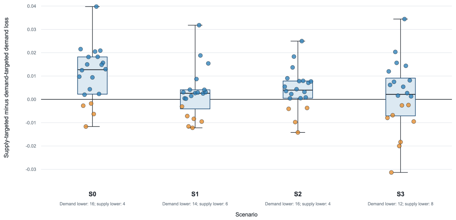
All 20 paired S0 results were retained. The demand-targeted search gave lower demand loss in 16 runs, while the supply-targeted search gave lower demand loss in four. The median relative reduction was 3.11%; the first and third quartiles were 0.55% and 4.35%, and the range was from −2.80% to 9.10%. The corresponding counts for S1, S2, and S3 were 14/6, 16/4, and 12/8. Figure 2 shows all paired run-level differences. These are descriptive results, not significance tests.

For six S0 seed pairs, the two search histories contained a candidate with lower demand loss than the final demand-targeted result. This included all four pairs in which the final supply-targeted result was lower. When each pair is represented by the lowest demand loss found anywhere in its two search histories, the supply-targeted side is not lower in any S0 pair. The selected candidate may come from either search, so this history check is not attributed to one strategy. The lowest reported demand losses for S0–S3 first appeared at generations 173, 200, 188, and 198, and the lowest reported supply loss first appeared at generation 195. These late improvements show why the reported analysis uses 200 rather than 20 generations.

Appendix B reports the run-to-run distributions and search history summary. Supplementary Data File S1 contains the complete run-level records.

5.3. GA Parameter Sensitivity and Number of Evaluated Schedules

The GA parameter analysis uses S0, the demand loss objective, and five preset random seeds. It compares the baseline P = 200 and E = 20 setting with P = 100 and E = 10, P = 300 and E = 30, crossover probability 0.8, mutation probability 0.05, and mutation probability 0.2. Every setting uses G = 200. The 25 new runs evaluate 905,000 schedules.

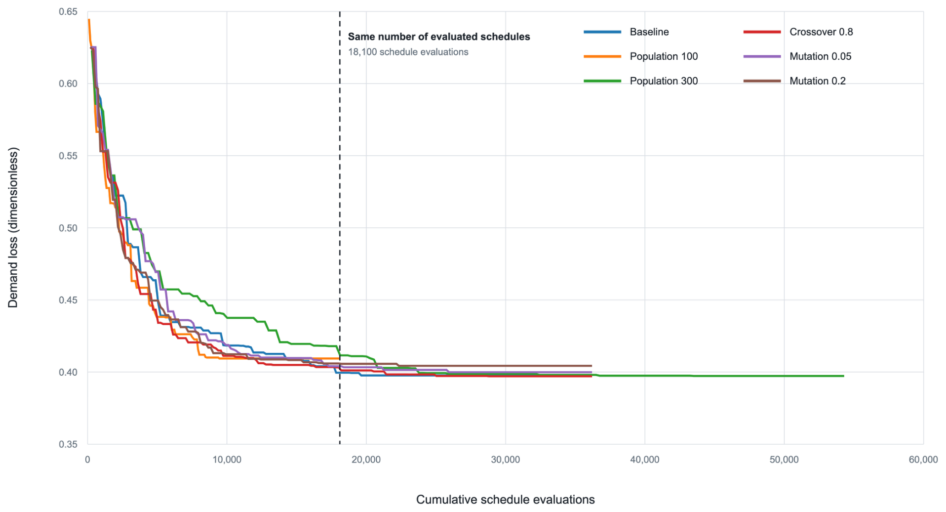
After 200 generations, P = 300 has the lowest five-run mean demand loss, 0.3963, compared with 0.3982 for the baseline, but it evaluates 54,300 schedules per run rather than 36,200. After the same 18,100 schedule evaluations, the baseline has the lowest mean, 0.4025, compared with 0.4143 for P = 300. The first comparison holds the number of generations constant; the second holds the number of evaluated schedules constant.

The analysis covers five runs for each setting. The observed ranking changes with the number of schedules evaluated.

Table 4. GA parameter sensitivity after 200 generations and after 18,100 schedule evaluations.

GA Setting	Population/Elites	Schedules Evaluated per Run	Mean Demand Loss After 200 Generations	Mean Demand Loss After 18,100 Evaluations	Total Time for Five Runs (s)
Baseline	200/20	36,200	0.3982 ± 0.0024	0.4025 ± 0.0067	1827.2
Population 100	100/10	18,100	0.4112 ± 0.0158	0.4112 ± 0.0158	962.9
Population 300	300/30	54,300	0.3963 ± 0.0023	0.4143 ± 0.0144	3232.8
Crossover 0.8	200/20	36,200	0.4007 ± 0.0065	0.4026 ± 0.0050	2087.7
Mutation 0.05	200/20	36,200	0.4043 ± 0.0094	0.4071 ± 0.0089	2032.9
Mutation 0.2	200/20	36,200	0.4051 ± 0.0049	0.4068 ± 0.0035	2050.0

Values are reported as the five-run mean ± sample standard deviation. Total elapsed time also covers five runs per setting. Displayed values are rounded; full-precision values are provided in Supplementary Data File S1.

reports the numerical summaries, and Figure 3 shows how the lowest demand loss changes as additional schedules are evaluated.

5.4. Comparison with a Deterministic Greedy Schedule

A deterministic greedy schedule is also constructed based on estimated demand benefit per crew day. At each decision point, the method ranks feasible task–mode pairs by their estimated demand–service benefit over the remaining horizon per crew day, and then starts the highest-ranked pair using a fixed tie rule. It continues until all 21 damaged tasks are scheduled.

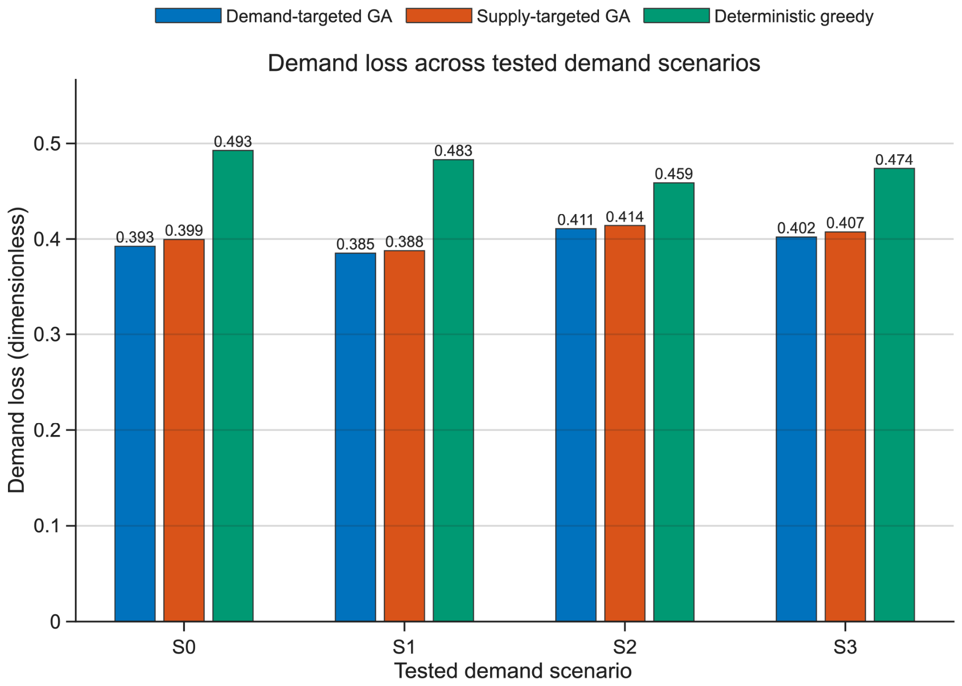
The deterministic greedy schedules have demand losses of 0.4927, 0.4831, 0.4586, and 0.4735 for S0–S3. The corresponding demand-targeted GA results are 0.3925, 0.3853, 0.4107, and 0.4021, which are 20.34%, 20.23%, 10.43%, and 15.09% lower.

Table 5. Demand loss comparison with the deterministic greedy schedule.

Scenario	Demand-Targeted GA	Supply-Targeted GA	Deterministic Greedy	Difference Between Demand-Targeted GA and Deterministic Greedy (%)
S0	0.3925	0.3995	0.4927	20.34
S1	0.3853	0.3880	0.4831	20.23
S2	0.4107	0.4140	0.4586	10.43
S3	0.4021	0.4073	0.4735	15.09

reports the numerical comparison, and Figure 4 shows the demand losses across the four scenarios. Supplementary Data File S1 provides full-precision supply loss, cumulative unmet demand, and average available supply.

The greedy method makes one choice at a time; it does not revise earlier decisions or jointly search the complete task order and mode vector. The GA result has lower demand loss in all four tested scenarios. However, each GA value is the lowest found across 20 runs, whereas the greedy method constructs one deterministic schedule. The computational effort, therefore, differs.

5.5. Sensitivity to Crew Availability, Repair Duration, and Demand Recovery Timing

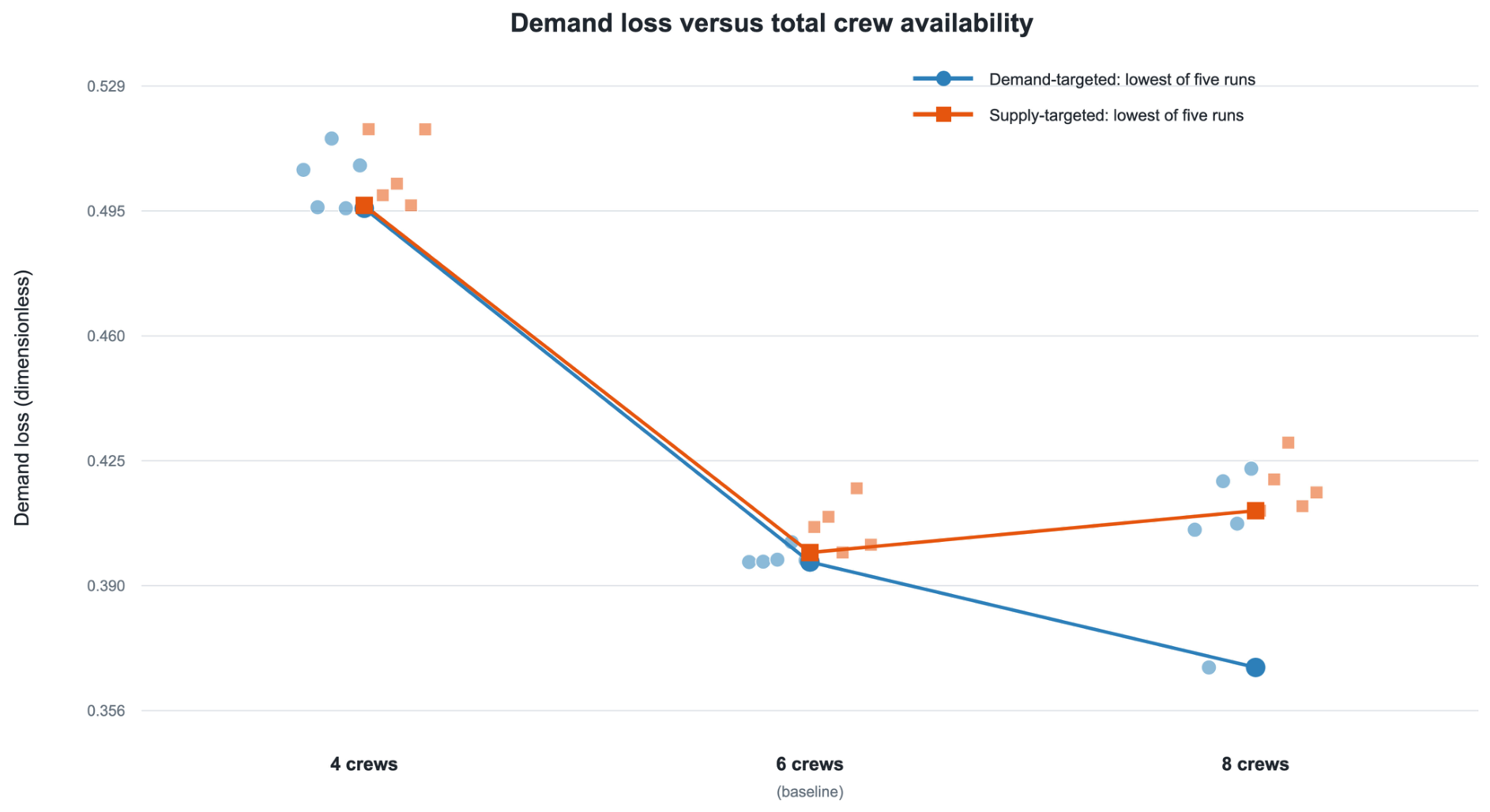
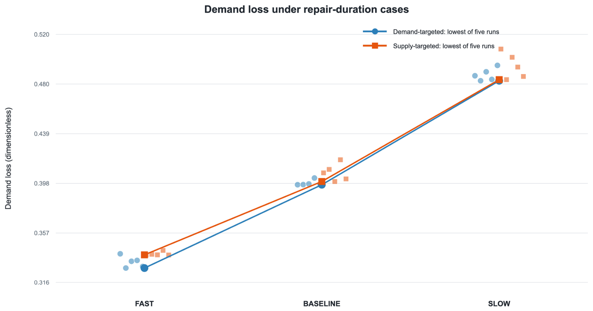
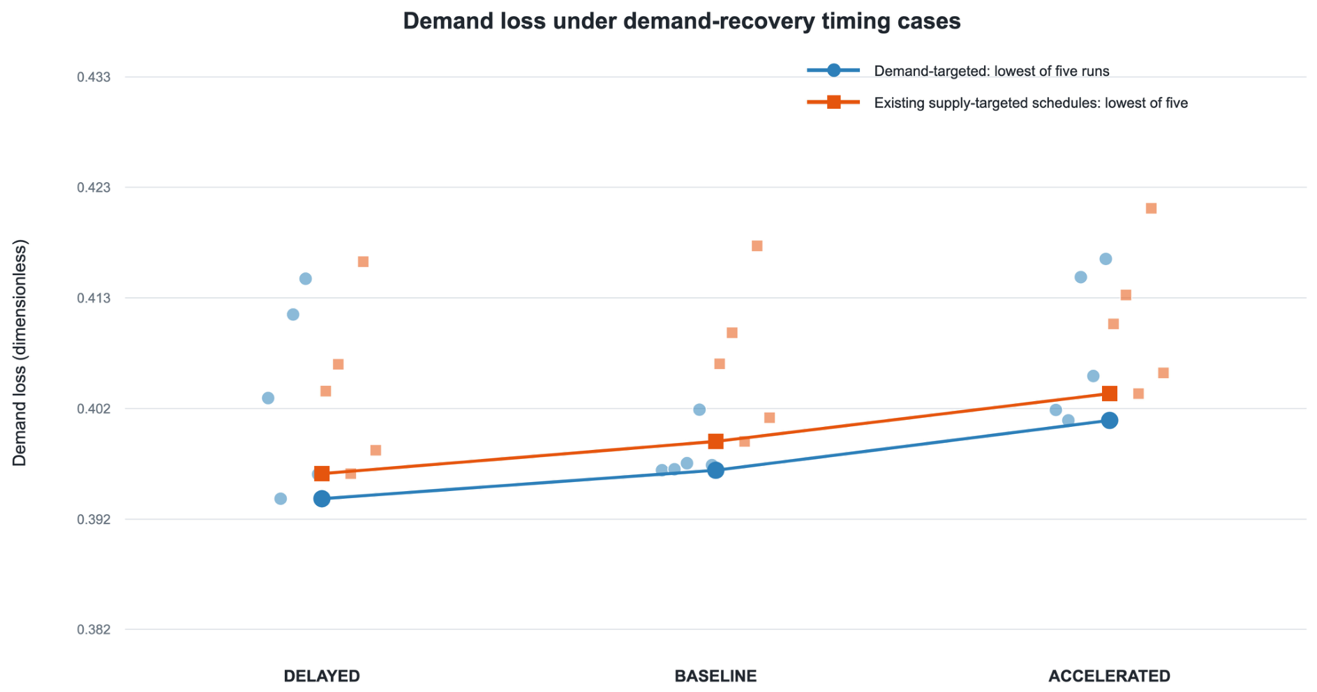
The sensitivity analysis changes crew availability, repair duration, and demand recovery timing separately on S0 using five preset random seeds. The six crew, baseline duration, and baseline timing cases use the same five baseline runs. Each additional GA run uses P = 200, E = 20, G = 200, and 36,200 schedules evaluated with the baseline operators. Figure 5, Figure 6 and Figure 7 and

Table 6. One-factor sensitivity to crew availability, repair duration, and demand recovery timing.

Factor	Level	Demand-Targeted Loss	Supply-Targeted Loss	Reduction vs. Supply-Targeted (%)	Change from Baseline (%)
Crew availability	4 crews	0.4953	0.4961	0.17%	24.80%
Crew availability	6 crews	0.3968	0.3995	0.66%	0.00%
Crew availability	8 crews	0.3675	0.4111	10.61%	−7.39%
Repair duration	Fast duration	0.3284	0.3392	3.21%	−17.26%
Repair duration	Baseline duration	0.3968	0.3995	0.66%	0.00%
Repair duration	Slow duration	0.4823	0.4832	0.19%	21.53%
Demand timing	Delayed by 2 days	0.3942	0.3965	0.58%	−0.65%
Demand timing	Baseline timing	0.3968	0.3995	0.66%	0.00%
Demand timing	Accelerated by 2 days	0.4014	0.4039	0.61%	1.15%

Displayed values are rounded; full-precision values are provided in Supplementary Data File S1. For Table 6, reduction vs. supply-targeted search (%) = 100 × (supply-targeted demand loss − demand-targeted demand loss)/supply-targeted demand loss. Change from baseline (%) = 100 × (level demand-targeted loss − baseline demand-targeted loss)/baseline demand-targeted loss. A negative change means a lower loss than the baseline.

summarize the results.

Crew availability is varied from the six crew baseline to four and eight crews, while retaining the maximum of three crews per task. Repair durations for the 21 damaged tasks are changed to max(1, ⌊0.8τ⌋) and ⌈1.2τ⌉; undamaged DS1 nodes remain zero-duration non-tasks. Demand timing is shifted two days later or earlier. When a shift extends beyond day 0 or day 14, the nearest boundary value is used. These are deterministic cases, not probability distributions.

Crew availability: The lowest demand losses found in five demand-targeted runs were 0.4953, 0.3968, and 0.3675 for four, six, and eight crews.

Repair duration: The lowest demand losses found in five runs were 0.3284, 0.3968, and 0.4823 for the fast, baseline, and slow cases.

Demand timing: The lowest demand-targeted losses found in five runs were 0.3942, 0.3968, and 0.4014 for delayed, baseline, and accelerated demand. Their cumulative system demands were 32,718, 34,114, and 35,495 kW-day, and the corresponding cumulative unmet demand was 12,899, 13,538, and 14,248 kW-day. Because the two-day shifts also change cumulative demand over the 14 objective intervals, both the numerator and denominator are provided in Supplementary Data File S1.

The sensitivity analysis does not vary damage severity, earthquake intensity, factor interactions, topology, the adopted node traversability rule, or dispatch. Damage severity and earthquake intensity would require a hazard-to-damage relationship that is not part of the present model.

The plotted and tabulated values are the lowest losses found in five runs at each level. A non-monotonic change can reflect both the changed model setting and variation between runs. Moving from six to four crews increases the lowest demand-targeted loss by 24.80%, while moving to eight crews reduces it by 7.39%. The fast duration case reduces loss by 17.26%, and the slow duration case increases it by 21.53%. Delaying demand changes loss by −0.65%, while accelerating it changes loss by 1.15%.

5.6. Runtime and Computational Environment

The four-scenario analysis included 115 GA runs and 4,163,000 schedules evaluated. Computation inside the GA took 41,417.5 s, and total elapsed time including run setup and output was 45,885.8 s. The parameter analysis added 25 runs and 905,000 schedules, with 10,366.4 s total elapsed time. The sensitivity analysis added 50 runs and 1,810,000 schedules, with 19,674.6 s total elapsed time. Across all reported GA analyses, 190 runs and 6,878,000 schedules were evaluated in MATLAB R2026a Update 3 on an Apple M5 Pro computer.

Runtime is reported separately for the four-scenario, parameter, and sensitivity analyses because baseline results are used in more than one comparison without being re-run. The times describe computational cost on the stated computer.

Table A6. Runtime and schedule evaluation summary.

Experiment	GA Runs	Schedule Evaluations	Total Elapsed Time (s)	What the Total Includes
Primary four-scenario experiment	115	4,163,000	45,885.8	Repeated demand- and supply-targeted searches
GA parameter analysis	25	905,000	10,366.4	Additional GA parameter runs
One-factor sensitivity analysis	50	1,810,000	19,674.6	Additional sensitivity runs
All reported GA experiments	190	6,878,000	—	—

Runtime values are reported separately for each experiment. Reuse of the baseline is not counted as a new GA run.

summarizes the totals, and Supplementary Data File S1 provides full-precision records.

6. Discussion

The lowest losses found across 20 runs and the paired run-level distribution answer different questions. The first shows the lowest value found by each search after the same number of schedules were evaluated; the second shows how results vary from one run to another. In all four S0 pairs where the final supply-targeted result was lower, the two search histories already contained a candidate with lower demand loss. Because that candidate may come from either search, the history check does not change the comparison between the two search strategies.

The GA result has lower demand loss than the deterministic greedy schedule in all four tested scenarios. The greedy method is much faster because it constructs one schedule rather than conducting 20 stochastic searches. This is a case-specific comparison, not a general ranking of methods.

The sensitivity results show larger demand loss changes across the tested crew and repair duration levels than across the two-day demand-timing shifts. Each factor is changed separately, so the results describe only the tested levels.

6.1. Practical Deployment Pathway

In a future deployment, the demand profiles used as model inputs could be updated from several operational sources. Advanced metering infrastructure (AMI) can provide interval consumption and outage/restoration indications. Supervisory control and data acquisition (SCADA) can provide network and equipment telemetry. Outage management systems (OMSs), distribution management systems (DMSs), and meter data management systems (MDMs) can combine outage tickets, device states, work orders, and validated meter streams. Building automation or energy management systems can provide building-side status where access is available, while inspection reports and crew updates can revise damage states and repair duration estimates [44,45,46,47,48]. Forecasting models could combine these observations with weather, occupancy, historical load, and restoration status to update demand profiles.

Operational use would also require explicit treatment of missing or delayed meter data, conflicting data sources, forecast error, communication latency, and the time needed to validate and assimilate updates. Meter and building data raise privacy, access control, and governance concerns, while SCADA, building automation, and other operational technology interfaces require cybersecurity, availability, and safety controls [44,45,47]. A rolling or event-triggered implementation could re-estimate the state and re-run the scheduler when material updates arrive, as conceptually related information update approaches do in other recovery models [49].

The present implementation uses fixed scenario matrices, topology, and dispatch rules. It does not connect directly to AMI, SCADA, OMS, DMS, MDM, building systems, inspection systems, forecasting services, or rolling re-optimization. The preceding workflow describes a possible future deployment, not a validated real-time controller.

6.2. Limitations

The results are conditional on an IEEE-33-derived illustrative network, fixed initial damage states, a one-to-one supply–demand mapping, no transfer of unused capacity, static open ties, no network reconfiguration, and a deterministic reachability-based supply model without power flow, voltage, line limits, or electrical losses. The damage functionality fractions, repair duration modes, six crew baseline, maximum three crews per task, and S0 demand profile are author-defined or fixed case study assumptions rather than universally calibrated engineering values. Exact repair durations and crew availability are deterministic within each case. The model omits crew travel, spare part logistics, uncertain inspection time, endogenous demand response, critical load or vulnerability weights, and distribution system operating constraints.

The repeated run results describe the schedules found under the stated stopping rules; they are not formal statistical inference or certified optimal solutions. The deterministic greedy schedule uses different computational effort. Crew availability, repair duration, and demand timing are changed separately. Damage severity, earthquake intensity, interactions, topology, dispatch, and alternative node traversability rules are outside the present analysis.

7. Conclusions

This study presents a demand-oriented repair scheduling model for the stated power-grid-building case study. With the same GA settings and number of schedules evaluated, the lowest baseline demand loss found in 20 demand-targeted runs was 0.3925, compared with 0.3995 for the supply-targeted search. This is a 1.7464% reduction and 238 kW-day less cumulative unmet demand. The supply-targeted result provides a 10.5 kW more average available supply, showing the trade-off between the two objectives. In a separate comparison with different computational effort, the demand-targeted GA result had 20.3% lower demand loss than one deterministic greedy schedule. Individual GA runs produced overlapping results. The parameter and sensitivity analyses also show that results depend on GA settings, crew availability, repair duration, and demand timing. The findings apply to the tested deterministic case study. Future work should calibrate demand and repair inputs, model power flow and switching, link hazard intensity to component damage, test interactions, and evaluate secure rolling re-optimization.

References

1. IEA. Global Energy Review 2025; International Energy Agency: Paris, France, 2025; Available online: https://iea.blob.core.windows.net/assets/5b169aa1-bc88-4c96-b828-aaa50406ba80/GlobalEnergyReview2025.pdf (accessed on 20 June 2025).
2. Coleman, N.; Esmalian, A.; Lee, C.C.; Gonzales, E.; Koirala, P.; Mostafavi, A. Energy inequality in climate hazards: Empirical evidence of social and spatial disparities in managed and hazard-induced power outages. Sustain. Cities Soc. 2023, 92, 104491. [Google Scholar] [CrossRef]
3. Nateghi, R.; Guikema, S.D.; Wu, Y.; Bruss, C.B. Critical assessment of the foundations of power transmission and distribution reliability metrics and standards. Risk Anal. 2016, 36, 4–15. [Google Scholar] [CrossRef] [PubMed]
4. Clark, S.S.; Peterson, S.K.; Shelly, M.A.; Jeffers, R.F. Developing an equity-focused metric for quantifying the social burden of infrastructure disruptions. Sustain. Resilient Infrastruct. 2023, 8, 356–369. [Google Scholar] [CrossRef]
5. Lee, C.C.; Maron, M.; Mostafavi, A. Community-scale big data reveals disparate impacts of the Texas winter storm of 2021 and its managed power outage. Humanit. Soc. Sci. Commun. 2022, 9, 124. [Google Scholar] [CrossRef] [PubMed]
6. Arif, A.; Wang, Z.; Wang, J.; Chen, C. Power distribution system outage management with co-optimization of repairs, reconfiguration, and DG dispatch. IEEE Trans. Smart Grid 2018, 9, 4109–4118. [Google Scholar] [CrossRef]
7. Tan, Y.; Qiu, F.; Das, A.K.; Kirschen, D.S.; Arabshahi, P.; Wang, J. Scheduling post-disaster repairs in electricity distribution networks. IEEE Trans. Power Syst. 2019, 34, 2611–2621. [Google Scholar] [CrossRef]
8. Yan, J.; Hu, B.; Xie, K.; Tai, H.M.; Li, W. Post-disaster power system restoration planning considering sequence dependent repairing period. Int. J. Electr. Power Energy Syst. 2020, 117, 105612. [Google Scholar] [CrossRef]
9. Pang, N.; Liu, H.; Huang, S.; Meng, J. Emergency rush repair task scheduling of distribution networks in large-scale blackouts. Int. J. Electr. Power Energy Syst. 2016, 82, 373–381. [Google Scholar] [CrossRef]
10. Zhu, H.; Xie, H.; Tang, L.; Fu, W.; Gao, J. Robust post-disaster repair crew dispatch for distribution systems considering the uncertainty of switches. Int. J. Electr. Power Energy Syst. 2024, 155, 109550. [Google Scholar] [CrossRef]
11. Song, X.; Zhao, P.; Yin, R.; Zu, Y.; Zhang, Y. Two-stage decision-dependent demand response driven by TCLs for distribution system resilience enhancement. Appl. Energy 2024, 361, 122894. [Google Scholar] [CrossRef]
12. Otsuka, A. Lessons from regional electricity demand change following natural disasters in Japan. Reg. Sci. Policy Pract. 2024, 16, 12631. [Google Scholar] [CrossRef]
13. Li, Y.; Xie, K.; Wang, L.; Xiang, Y. Exploiting network topology optimization and demand side management to improve bulk power system resilience under windstorms. Electr. Power Syst. Res. 2019, 171, 127–140. [Google Scholar] [CrossRef]
14. Jalilpoor, K.; Nikkhah, S.; Sepasian, M.S.; Ghobadi Aliabadi, M. Application of precautionary and corrective energy management strategies in improving networked microgrids resilience: A two-stage linear programming. Electr. Power Syst. Res. 2022, 204, 107704. [Google Scholar] [CrossRef]
15. Liu, Z.; Du, Y.; Yi, J.; Liang, F.; Ma, T.; Pei, T. Quantitative Association between Nighttime Lights and Geo-Tagged Human Activity Dynamics during Typhoon Mangkhut. Remote Sens. 2019, 11, 2091. [Google Scholar] [CrossRef]
16. Li, Y.; Xiao, F.; Zhang, X.; Gao, W.; Ruan, Y.; Zhou, N.; Kammen, D.M. Extreme typhoon events trigger long-lasting power outages and require demand-side solutions to enhance energy resiliency. Commun. Earth Environ. 2025, 6, 136. [Google Scholar] [CrossRef]
17. Handa, Y.; Opabola, E.; Galasso, C. A Bayesian approach for estimating the post-earthquake recovery trajectories of electric power systems in Japan. Sustain. Resilient Infrastruct. 2024, 9, 407–420. [Google Scholar] [CrossRef]
18. Sun, L.; Stojadinovic, B.; Sansavini, G. Agent-based recovery model for seismic resilience evaluation of electrified communities. Risk Anal. 2019, 39, 1597–1614. [Google Scholar] [CrossRef] [PubMed]
19. Didier, M.; Broccardo, M.; Esposito, S.; Stojadinovic, B. A compositional demand/supply framework to quantify the resilience of civil infrastructure systems (Re-CoDeS). Sustain. Resilient Infrastruct. 2018, 3, 86–102. [Google Scholar] [CrossRef]
20. Jiang, X.; Chen, J.; Chen, M.; Wei, Z. Multi-stage dynamic post-disaster recovery strategy for distribution networks considering integrated energy and transportation networks. CSEE J. Power Energy Syst. 2021, 7, 408–420. [Google Scholar] [CrossRef]
21. Zhang, Z.; Zhou, K.; Yang, S. A post-disaster load supply restoration model for urban integrated energy systems based on multi-energy coordination. Energy 2024, 303, 132008. [Google Scholar] [CrossRef]
22. Canbilen Sütiçen, T.; Batun, S.; Çelik, M. Integrated reinforcement and repair of interdependent infrastructure networks under disaster-related uncertainties. Eur. J. Oper. Res. 2023, 308, 369–384. [Google Scholar] [CrossRef]
23. Bruneau, M.; Chang, S.E.; Eguchi, R.T.; Lee, G.C.; O’Rourke, T.D.; Reinhorn, A.M.; Shinozuka, M.; Tierney, K.; Wallace, W.A.; von Winterfeldt, D. A framework to quantitatively assess and enhance the seismic resilience of communities. Earthq. Spectra 2003, 19, 733–752. [Google Scholar] [CrossRef]
24. Holling, C.S. Resilience and stability of ecological systems. Annu. Rev. Ecol. Syst. 1973, 4, 1–23. [Google Scholar] [CrossRef]
25. Amirioun, M.H.; Aminifar, F.; Lesani, H.; Shahidehpour, M. Metrics and quantitative framework for assessing microgrid resilience against windstorms. Int. J. Electr. Power Energy Syst. 2019, 104, 716–723. [Google Scholar] [CrossRef]
26. Bie, Z.; Lin, Y.; Li, G.; Li, F. Battling the extreme: A study on the power system resilience. Proc. IEEE 2017, 105, 1253–1266. [Google Scholar] [CrossRef]
27. Jia, C.; Zhang, L.; Wang, Z. Joint pre- and post-disaster planning to enhance the resilience of critical infrastructures. Reliab. Eng. Syst. Saf. 2023, 231, 109023. [Google Scholar] [CrossRef]
28. Mohanty, A.R.; Ramasamy, A.K.; Verayiah, R.; Bastia, S.; Dash, S.S.; Cuce, E.; Khan, T.M.Y.; Soudagar, M.E.M. Power system resilience and strategies for a sustainable infrastructure: A review. Alex. Eng. J. 2024, 105, 261–279. [Google Scholar] [CrossRef]
29. Vijay, S.; De, M. Power distribution system resilience: A perspective of the power system operator. Sustain. Energy Grids Netw. 2025, 44, 101950. [Google Scholar] [CrossRef]
30. Hadi, M.; Elbouchikhi, E.; Zhou, Z.; Saim, A. Optimal energy management in multi-energy microgrid with combined heat and power system and demand side response integration. Renew. Energy 2026, 256, 124076. [Google Scholar] [CrossRef]
31. Mozaffari, M.; Abedini, M.; Monsef, H.; Marzband, M. Stochastic modeling and techno-economic optimization for distribution network resilience under extreme events with integration of electric vehicles. Sustain. Energy Grids Netw. 2026, 47, 102351. [Google Scholar] [CrossRef]
32. Shafiei, K.; Roudnil, S.; Ghassem Zadeh, S. Power system resilience: Optimal risk-based planning with renewable energy sources and energy storage systems. Energy Convers. Manag. X 2026, 30, 101879. [Google Scholar] [CrossRef]
33. Shafiei, K.; Seifi, A.; Tarafdar Hagh, M. A novel multi-objective optimization approach for resilience enhancement considering integrated energy systems with renewable energy, energy storage, energy sharing, and demand-side management. J. Energy Storage 2025, 115, 115966. [Google Scholar] [CrossRef]
34. Chung, I.B.; Luo, Y.; Wang, P.F. Data-driven co-design of power distribution networks for resilience enhancement through graph neural network-aided performance estimation. Reliab. Eng. Syst. Saf. 2026, 272, 112511. [Google Scholar] [CrossRef]
35. Liang, H.; Moya, B.; Chinesta, F. Resilience-based post-disaster recovery optimization for infrastructure system via deep reinforcement learning. Reliab. Eng. Syst. Saf. 2026, 265, 111478. [Google Scholar] [CrossRef]
36. Li, J.; Wang, X.; Liu, Y.; Zhang, H. Enhancing interdependent infrastructure systems resilience in post-disaster recovery: A social-technical approach based on reinforcement learning. Sustain. Cities Soc. 2026, 148, 107608. [Google Scholar] [CrossRef]
37. Zhang, Z.; Li, Y.; Wang, X.; Liu, P. Mechanism-driven resilience modeling and assessment of power system under high-power microwave disturbances. Reliab. Eng. Syst. Saf. 2026, 276, 112933. [Google Scholar] [CrossRef]
38. Mackie, K.R.; Wong, J.M.; Stojadinović, B. Post-earthquake bridge repair cost and repair time estimation methodology. Earthq. Eng. Struct. Dyn. 2010, 39, 281–301. [Google Scholar] [CrossRef]
39. Li, D.; Li, L.; Luo, T.; Zhou, M.; Huang, S. Optimization method for power supply restoration under flood disasters. In Proceedings of the 2025 8th International Conference on Algorithms, Computing and Artificial Intelligence (ACAI); IEEE: Piscataway, NJ, USA, 2025; pp. 1–5. [Google Scholar] [CrossRef]
40. Zhou, Z.; Ma, J.; Huang, Y.; Liang, L.; Chen, Z. Intelligent optimisation of self-healing strategy of distribution network based on differential evolution and advanced fractal. Int. J. Dyn. Syst. Differ. Equ. 2025, 14, 64–81. [Google Scholar] [CrossRef]
41. Katoch, S.; Chauhan, S.S.; Kumar, V. A review on genetic algorithm: Past, present, and future. Multimed. Tools Appl. 2021, 80, 8091–8126. [Google Scholar] [CrossRef] [PubMed]
42. Naghavi, M.; Yousefi Joobeni, A.; Mirhosseini, M.; Dashti, R. Optimal siting and sizing of energy storage systems for enhancing smart grid resilience using genetic algorithm. J. Energy Storage 2026, 154, 121196. [Google Scholar] [CrossRef]
43. Baran, M.E.; Wu, F.F. Network reconfiguration in distribution systems for loss reduction and load balancing. IEEE Trans. Power Deliv. 1989, 4, 1401–1407. [Google Scholar] [CrossRef]
44. NIST SP 1108r4; NIST Framework and Roadmap for Smart Grid Interoperability Standards, Release 4.0. National Institute of Standards and Technology: Gaithersburg, MD, USA, 2021. [CrossRef]
45. NIST SP 800–82r3; Guide to Operational Technology Security. National Institute of Standards and Technology: Gaithersburg, MD, USA, 2023. [CrossRef]
46. Office of Electricity; U.S. Department of Energy. A System in Transition: The Influence of Next Generation Technologies; U.S. Department of Energy: Washington, DC, USA, 2022. Available online: https://www.energy.gov/oe/articles/system-transition-report (accessed on 30 July 2026).
47. National Institute of Standards and Technology. Guidelines for Smart Grid Cybersecurity; NISTIR 7628 Revision 1; National Institute of Standards and Technology: Gaithersburg, MD, USA, 2014. [CrossRef]
48. Office of Electricity; U.S. Department of Energy. Grid Modernization and the Smart Grid. Available online: https://www.energy.gov/oe/grid-modernization-and-smart-grid (accessed on 30 July 2026).
49. Wan, H.; Liu, W.; Shi, Q.; Zhang, Y.; Wang, Y.; Zhang, S. Multi-time-step rolling optimization strategy for post-disaster emergency recovery in distribution system based on model predictive control. CSEE J. Power Energy Syst. 2025, 11, 243–254. [Google Scholar] [CrossRef]
Figure 1. IEEE-33-derived radial supply network and initial damage state used in the case study. Solid lines are the 32 active radial edges; dashed lines with crosses are the five normally open ties. Each supply node serves one paired demand node under the fixed one-to-one dispatch rule.
Mathematics 14 02855 g001
Figure 2. Paired demand loss differences across S0–S3. The plotted value is supply-targeted minus demand-targeted demand loss, so values above zero favor the demand-targeted run. All 20 paired results are shown for each scenario. Blue markers indicate cases in which the demand-targeted run has lower demand loss, while orange markers indicate cases in which the supply-targeted run has lower demand loss.
Mathematics 14 02855 g002
Figure 3. Median lowest demand loss found as the number of evaluated schedules increases, based on five runs per GA setting. The dashed line marks 18,100 schedule evaluations, where all settings can be compared after the same amount of search.
Mathematics 14 02855 g003
Figure 4. Demand loss across S0–S3 for demand-targeted GA search, supply-targeted GA search, and the deterministic greedy schedule. Each GA value is the lowest found across 20 runs; the greedy method constructs one schedule using different computational effort.
Mathematics 14 02855 g004
Figure 5. Demand loss at total crew availabilities of 4, 6, and 8. Pale markers show the five runs; solid markers show the lowest loss found for each objective.
Mathematics 14 02855 g005
Figure 6. Demand loss under fast, baseline, and slow deterministic repair duration cases. Pale markers show the five runs; solid markers show the lowest loss found for each objective.
Mathematics 14 02855 g006
Figure 7. Demand loss under delayed, baseline, and accelerated demand timing. For the delayed and accelerated cases, the existing S0 supply-targeted schedules are re-evaluated because the supply objective does not depend on the demand profile; no additional supply-targeted GA run is required.
Mathematics 14 02855 g007