Quality Investment and Green Disclosure Strategy in Competitive Supply Chains Considering Customer Trust

Abstract

Purpose: This paper investigates how product quality and green information transparency jointly influence customer trust in green products and examines competing retailers’ green disclosure and suppliers’ quality investment strategies under information asymmetry. Methodology: We develop a game-theoretic model of two competing retailers and two suppliers with asymmetric quality investment costs. We characterize equilibrium outcomes in sequential disclosure games and study the effects of the trust factor and transparency level on the equilibrium outcomes. Findings: Three main results emerge. First, a second-mover advantage exists in sequential disclosure, namely, the later retailer free-rides on the first mover’s information. Second, higher trust intensifies competition by homogenizing customer utility, whereas greater transparency softens competition by making valuations more heterogeneous. Third, customer trust can incentivize both retailers to disclose simultaneously. Novelty: First, this paper studies consumers’ heterogeneous green preferences and considers the information asymmetry of green attributes between supply and demand. Second, this paper determines the suppliers’ quality investment considering the retailers’ strategic green disclosure and constructs the endogenous trust function. Third, this paper analyzes the retailers’ green disclosure in equilibrium, further determines the market coverage, and points out the effects of key parameters on the market coverage and the product competition.

1. Introduction

Product quality as the foremost factor affects customers’ trust (https://www.prnewswire.com/news-releases/consumers-will-pay-a-premium-for-brands-they-trust-salsify-finds-in-new-consumer-research-301238179.html accessed on 26 July 2026); the positive effects on brand trust from product quality can further affect the customers’ willingness to pay [1]. Green products are typical trust-based goods; consumers often find it challenging to verify the authenticity of a product’s green attributes, even after purchasing and using it. Green products inherently create quality information asymmetry between supply and demand, leading customers to develop a perception of product quality. By offering thorough and transparent information about product characteristics and origins, stakeholders can distinguish themselves from competitors while fostering trust and stimulating demand. Environmental information transparency increases trust and further increases purchase intention [2,3]. Nowadays, more and more platform retailers are disclosing product information. In September 2025, JD Qixian launched its self-developed food safety and quality traceability system. Consumers can scan the QR code or click on the product page of the app to lock in the purchased batch of goods and observe the real-time data of the entire chain from the place of origin, to the logistics warehouse, and to the store (https://baijiahao.baidu.com/s?id=1861405822047915263&wfr=spider&for=pc accessed on 26 July 2026). By collaborating with IBM Product Trust, Carrefour can utilize blockchain to offer customers unparalleled transparency regarding the movement of their food (https://www.ibm.com/blockchain/resources/food-trust/grocery/ accessed on 26 July 2026). Additionally, the quality of information enhances and reinforces the connections between electric vehicle-related data, perceived value, and trust [4].

The costs of information disclosure such as chemical composition information provided by sensors hinder information disclosure [5]. Niu et al. [6] studied the issue of reducing customers’ quality untrust towards the remanufactured product by adopting blockchains. Lv and Bi [7] investigate the role of blockchain technology in combating greenwashing involving manufacturers of low- and high-carbon products; the model integrates consumers’ low-carbon preference, consumer trust and product green level. However, the parameter about trust in the above research is fixed at value. This paper constructs the trust function by combining product quality and information transparency and further incorporates the trust function into the customer utility function, which reflects the customers’ willingness to purchase products. We specifically solve the following problems.

(a) What are the optimal quality investments for the suppliers?

(b) What are the retailers’ information strategies under competition in equilibrium?

(c) How does the customers’ trust made up of product quality and information transparency affect the related decisions, such as the market coverage and product competition?

To answer these questions, we analyze the setting where two competitive retailers sell products with uncertain quality information to customers; the retailers can determine whether to adopt information disclosure strategies or not based on profit comparison before and after information disclosure. Two suppliers are responsible for two products’ quality investment, and both product quality and information transparency can affect customers’ trust, which further affects customers’ willingness to pay. Supplier 1 is more cost-effective in quality investment than supplier 2, and retailer 1 who transacts with supplier 1 makes information disclosure and pricing strategies prior to retailer 2, who transacts with supplier 2. This paper contributes to the prior literature in the following aspects. First, this paper studies consumers’ heterogeneous green preferences and considers the information asymmetry of green attributes between supply and demand. Second, this paper determines the suppliers’ quality investment considering the retailers’ strategic information disclosure and constructs the endogenous trust function. Third, this paper analyzes the retailers’ information disclosure in equilibrium, further determines the market coverage, and points out the effects of key parameters on the market coverage and the product competition. This paper finds that there exists a second mover advantage in a sequential information disclosure game. The effects of trust factor and information transparency on the competition between two retailers show the opposite trend, that is, a higher trust factor enhances the intensity of competition by making customers’ utility homogeneous, whereas a higher information transparency level makes the customers’ valuations about the products heterogeneous and hence softens the competition. Customers’ trust can urge two retailers to achieve (disclosure, disclosure) equilibrium. This paper suggests the retailer transacting with the supplier inefficient in quality investment discloses information, whereas the fiercer quality competition caused by increased trust factor has a detrimental effect on supplier 2. In the information strategy (disclosure, disclosure), retailer 2 can gain more advantages in market share than retailer 1 through information disclosure when the level of information disclosure is relatively high.

The remainder of this paper is structured as follows: Section 2 examines the relevant literature, while Section 3 presents the model assumptions and develops the framework. Section 4 determines the equilibrium decisions about pricing and quality investment under retailers’ different information strategies. Section 5 derives two retailers’ information disclosure strategies in equilibrium, determines market coverage under different information strategies, and explores the impacts of key parameters on optimal decisions. Last, Section 6 summarizes the study, points out implications and outlines directions for future research.

2. Literature Review

This paper is mainly related to the following streams of literature: (1) green investment in competitive supply chains, (2) green disclosure in the supply chain, and (3) the role of green information in building trust.

2.1. Green Investment in Competitive Supply Chains

In downstream competitive settings, Ma and He [8] investigated optimal green investment strategies within a green tourism supply chain and indicated that both investment intensity and sustainability levels rise alongside stronger tourist preferences for green travel. From an upstream competition perspective, Zhang et al. [9] showed that while manufacturers’ green investments can enhance retailer performance, such investments may fail to yield manufacturer profits when costs become excessively high. Zhang et al. [10] further highlighted the strong interdependence between green innovation and quality-related investment in corporate decision-making. Yang et al. [11] demonstrated that manufacturers may still engage in green technological investment even under weak environmental sensitivity, independent of rivals’ strategic behavior. Hafezi et al. [12] reported that both standalone and cost-sharing investment modes may lead to suboptimal environmental outcomes, depending on competitive pricing pressure and demand sensitivity to quality.

Regarding supply chain competition, Adnan et al. [13] examined competing electric vehicle supply chains and found that manufacturers must balance higher revenue from greener technologies against increased investment burdens. From a dual-channel viewpoint, Li et al. [14] analyzed manufacturer encroachment decisions in channels featuring substitutable green products, concluding that stronger consumer environmental awareness and higher substitutability improve manufacturer profitability. Zong et al. [15] proposed a platform-based supply chain model and showed that reduced efficiency in green investment shifts distribution strategies from marketplace-based channels toward dedicated green product lines. Finally, Zhang et al. [16] investigated product line strategies in competing manufacturing firms and observed a tendency toward convergence on green product offerings, even when conventional product lines may generate higher profits.

The research about green investment in competitive supply chains involves downstream, upstream, supply chain competition, and channel decisions. Although the effects of quality on the customers’ product trust have been revealed [1,14,17], the research incorporating quality investment into the product trust and further constructing the related customer utility function is few. This paper considers the endogenous product quality, further forms the trust function, and integrates it into the customers’ utility function.

2.2. Green Disclosure in the Supply Chain

In the context of retailer disclosures, Cai et al. [18] noted that suppliers typically prefer mandatory disclosure, while retailer preferences depend on wholesale prices and the demand impact of greenness. Ma et al. [19] investigated manufacturers’ investments in green emission reductions and retailers’ commitments to information disclosure technology aimed at enhancing product greenness perception. Chen and Duan [20] examined supply chain greenwashing, finding that retailers may reveal unethical supplier information if it significantly benefits NGOs targeting these suppliers.

Regarding manufacturer disclosures, Hong et al. [21] determined that mandatory quality information disclosure can boost profits for members of closed-loop supply chains when a green manufacturer utilizes third-party quality assessments. Wang et al. [22] applied negative binomial regression to demonstrate that excessive green knowledge can impede innovation efficiency in supply chains.

In terms of blockchain disclosures, Li et al. [23] uncovered that carbon signals create stronger incentives for high-potential manufacturers to hide their capabilities compared with sales signals. Zhou et al. [24] indicated that blockchain-enabled disclosures enhance consumer trust in sustainability initiatives. He et al. [5] explored strategies for offering green products, concluding that exclusive production of green products is the most profitable. Hsieh et al. [25] showed that manufacturers are more inclined to adopt blockchain when offered by the incumbent platform, particularly as cross-channel influences rise.

From a retailer’s perspective, Guo et al. [26] studied the adoption of eco-labels and blockchain for environmental disclosures in the fashion sector. Yao et al. [27] analyzed how platforms use blockchain to reveal manufacturer practices, noting a shift in preference from a reselling model to an agency model as consumer acceptance increases.

Although information transparency has been confirmed to affect the customers’ trust and can further affect customers’ willingness to pay, the study deriving the customers’ demand by considering the effects of the customers’ trust on the demand is few. This paper fills this research gap, and this also constitutes one of the contributions; meanwhile, the above research rarely considers heterogeneous green preferences of customers.

2.3. The Role of Green Information in Building Trust

Fu et al. [2] demonstrated that production technology and means transparency influence consumer trust in distinct ways, affecting competence and benevolence. Following this, Fu et al. [3] emphasized that transparency in production and environmental information boosts consumer trust and enhances purchase intentions. However, greenwashing leads to an increase in consumer skepticism towards green claims [28].

From the perspective of blockchain, regarding the benefits of implementing blockchain, Liu et al. [29] investigated how consumer familiarity with blockchain technology and perceived environmental information transparency foster digital and swift trust, which subsequently affects impulse buying behavior. Duong et al. [30] noted that blockchain transparency positively impacts consumer attitudes and intentions toward purchasing organic foods. Likewise, Zhang et al. [31] found that blockchain improves consumer trust through greater transparency, although its economic benefits hinge on implementation costs and consumer understanding, especially in the green food sector [32,33]. Cheng et al. [34] revealed that the use of blockchain-enabled smart contracts correlates positively with relationship governance elements, influencing information sharing, integration management, and relationship quality to varying degrees. It can enhance consumer confidence in sustainable products and improving demand prediction accuracy [35] and can increase profits for all parties involved in the green supply chain [36].

However, Lv and Bi [7] found that the implementation of blockchain technology by a low-carbon product manufacturer leads to a decrease in product green level. Lu et al. [37] found that blockchain’s adoption and imposing an investment cap on the product’s green degree have little effect on profitability for suppliers, manufacturers, logistics providers, and third-party platforms; an increase in blockchain implementation costs can lead to higher prices for low-carbon products [38].

Transparency can enhance consumer trust and purchase intention, but green washing will weaken this effect. Although blockchain can enhance transparency and promote trust, its actual benefits are constrained by factors such as implementation costs, consumer awareness, and product greenness, and the effect is not necessarily positive. Currently, there is little research on green information disclosure that considers the heterogeneity of consumer green preferences.

To sum up, this paper studies the issue of customer trust effect by combining retailers’ information disclosure and product quality, which is improved by the suppliers’ quality investment, and constructs the endogenous trust function. In addition to that, this paper analyzes the retailers’ information disclosure in equilibrium, further determines the market coverage, and points out the effects of key parameters on market coverage and product competition.

Table 1. A summary of the literature.

Literature	Heterogeneous Green Preferences	Information Disclosure	Consumer Trust	Supply Chain	Competition
Adnan et al. [13]				✓	✓
Cai et al. [18]		✓		✓
Chen et al. [20]		✓		✓
Guo et al. [26]		✓		✓
Hafezi et al. [12]					✓
He et al. [35]		✓	✓	✓
He et al. [5]		✓			✓
Hong et al. [21]		✓		✓
Hsieh et al. [25]		✓		✓	✓
Li et al. [14]				✓	✓
Li et al. [23]		✓		✓
Lu et al. [37]				✓
Lv and Bi [7]			✓		✓
Ma and He [8]				✓	✓
Wang et al. [22]				✓	✓
Zhang et al. [16]				✓	✓
Zhou et al. [24]		✓	✓	✓	✓
Zong et al. [15]				✓	✓
This paper	✓	✓	✓	✓	✓

reveals that the studies have combined information disclosure and consumer trust in the supply chain; they rarely consider customers’ heterogeneous green preferences.

3. Model Description

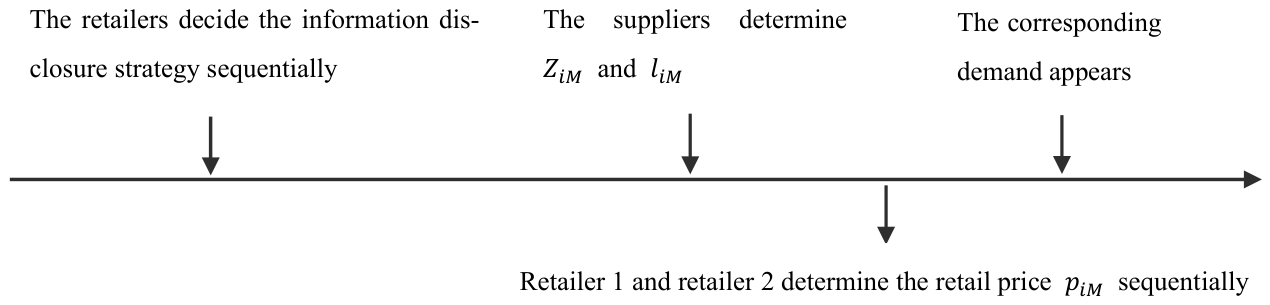
We analyze two supply chains, each comprising a single retailer and a supplier, as shown in Figure 1. We assume the suppliers are the leaders, and the retailers are the followers. The supplier determines the quality investment $Z_{iM}$ ($i=1 or 2$, $M\in \{dn,dd,nd,nn\})$ under the information strategy $M$, the wholesale price charged to retailer $i$ is $l_{iM}$, and the retailer offers products to customers at the price $p_{iM}$; the research setting can refer to Ma and He [8] and Hsieh et al. [25]. Since information disclosure is a long-term decision, as Figure 1 shows, two retailers make information disclosure decisions before the selling season begins. Two suppliers determine the quality investments and the corresponding wholesale prices; then, two retailers determine the retail prices. Using backwards reduction, retailer 2 and retailer 1 determine $p_{2M}$ and $p_{1M}$, respectively. Then, two suppliers determine $l_{iM}$ and $Z_{iM}$ simultaneously.

3.1. Product Quality Function with Quality Investments

Similar to the prior literature (e.g., Wang and Li [39]), we assume that quality function of the product after supplier $i^{\prime }s$ investment is $Z_{iM}$, and the corresponding cost will be ${\displaystyle \frac{{\zeta }_i}{2}}{Z_{iM}}^2(i=1 or 2)$, where ${\zeta }_i>0$ is the quality investment cost coefficient. Similar to the previous studies (e.g., Liu et al. [40]), this cost function reflects the diminishing performance of quality investment. As the coefficient for quality investment costs increases, the efficiency of quality investments decreases. To emphasize the impact of differences in quality investments on decision-making, we assume that the cost difference of quality investments is large enough, namely, $\delta ={\displaystyle \frac{{\delta }_2}{{\delta }_1}}>{\displaystyle \frac{\left(\lambda +13\tau \right)}{\left(11\tau -\lambda \right)}}$, which can avoid trivial conditions.

3.2. Customers’ Trust

$\lambda$ is the basic customer trust; Chen et al. [41] assumed that the additional trust utility of direct seller relative to reseller is fixed at value. According to the literature concluded in Section 2.3, customers’ product trust is mainly determined by the product quality and information transparency. Product quality as the foremost factor affects customers’ trust (https://www.prnewswire.com/news-releases/consumers-will-pay-a-premium-for-brands-they-trust-salsify-finds-in-new-consumer-research-301238179.html accessed on 26 July 2026), which can further affect the customers’ willingness to pay [1]. This paper assumes that the customers’ product trust can be denoted by $\left(\rho +Z_{iM}\right)\lambda$, which is positively correlated with product quality and information transparency level. If the retailer does not disclose information, i.e., $\rho =0$, the customers’ trust will be $Z_{iM}\lambda$ rather than 0 due to the fact that customers in this context can still obtain additional trust utility from product quality [17,42]; we hence use additive functions rather than multiplicative functions to describe customers’ product trust. Basic customer trust can be measured by using validated Likert-scale instruments from the prior marketing literature [42,43].

3.3. Customers’ Utility Function Under Asymmetric Information

Following Zhang et al. [44] and Sui et al. [45], we assume that the basic valuation of the products by the customer is denoted as $v$. These customers differ in their green preference for two retailers’ products, which is characterized by $x$ and obeys the uniform distribution on (0, 1) ($x\in \left[\mathrm{0,1}\right]$). In alignment with Zhang et al. [44], this paper assumes that the retailers can know the distribution of customers’ preferences. Based on the research of Lv and Li [46], consumer preferences for green products exhibit heterogeneity. Specifically, Lv and Li [46] categorized product attributes into vertical quality attributes and horizontal green attributes. Therefore, this article assumes that customers’ green preferences are horizontally heterogeneous, and there exists variant-misfit probability when making purchase decisions. Without loss of generality, we position retailer 1 at $x=0$ and retailer 2 at $x=1$. A customer located at preference point $x$ faces a misfit cost of $\tau x$ when buying from retailer 1 and a cost of $\tau (1-x)$ when buying from retailer 2. If customers purchase the products that do not match green preferences, it will weaken the customers’ utility due to the mismatch costs. Green products are typically trust-based goods; consumers often find it challenging to verify the authenticity of a product’s green attributes, even after purchasing and using it. Green products inherently create quality information asymmetry between supply and demand, leading customers to develop a perception of product quality. When retailers disclose green information, following Kwark et al. [47], the information is denoted by a signal $s$, which accurately indicates the true extent of the mismatch or provides effective information with a probability of $\rho$ and indicates the false extent of the mismatch or provides ineffective information with a probability of $1-\rho$. When the signal satisfies $s=x$, the customer’s expectation of $x$ can be expressed as ${\displaystyle \frac{1-\rho }{2}}+\rho x$. Following Kwark et al. [47] and Zhang et al. [44], this paper denotes the value of $\overline{x}$ as $y$, and the corresponding probability density function is $P\left(s=x|\overline{x}=y\right)=\left(1-\rho \right)+\rho \delta \left(x-y\right)$, where $\delta \left(z\right)$ is the Dirac delta distribution satisfying ${\int }_{-\infty }^{\infty }\delta \left(z\right)dz=1$ and $\delta \left(z\right)=\left\{\begin{array}{cc}0& z\ne 0\\ \begin{array}{c} \\ \infty \end{array}& z=0\end{array}\right.$. The conditional expectation is $P\left(\overline{x}=y|s=x\right)={\displaystyle \frac{P\left(s=x|\overline{x}=y\right)P\left(\overline{x}=y\right)}{P\left(s=x\right)}}=1-\rho +\rho \delta \left(x-y\right)$. The customer’s expectation of $\overline{x}$ condition on the signal $s=x$ can be expressed as $E\left(\overline{x}|s=x\right)={\int }_0^{1}yP\left(\overline{x}=y|s=x\right)dy={\int }_0^{1}y\left(1-\rho +\rho \delta \left(x-y\right)\right)dy={\int }_0^{1}y\left(1-\rho \right)dy+{\int }_0^1\rho \delta \left(x-y\right)ydy={\displaystyle \frac{1-\rho }{2}}+\rho x$.

Table 2. Notation and definitions.

Notation	Definitions
$v$	Customer valuations of the product
$x$	Location of an individual customers’ preference and obeys the uniform distribution on [0, 1]
$x_{iM}$	Perceived mismatch degree to product $i$ in scenario $M$
$s$	The signal which shows the actual extent of the mismatch
$\tau$	Unit misfit cost
$p_{iM}$	The selling price of product $i$ in scenario $M$, $i\in \{1, 2\}$, $M\in \{dn,dd,nd,nn\}$
$l_{iM}$	The wholesale price of product $i$ in scenario $M$
$Z_{iM}$	Product quality after supplier $i$’s investment
$\rho$	Information disclosure level
$F$	The cost of information disclosure for the retailer
$E\left(U_{iM}\right)$	Customer’s ex-ante utility in scenario $M$ when purchasing product $i$, $i=1 or 2$, $M=\left\{dn,dd,nn,nd\right\}$
$D_{iM}$	Total customer demand of product $i$ in scenario $M$
${\pi }_{jiM}$	The expected profit of member $j$ in scenario $M$, $j=\left\{l,r\right\}$, $M=\left\{dn,dd,nn,nd\right\}$

shows the notation and definitions in this paper.

4. The Optimal Decisions Under Retailers’ Different Information Strategies

To obtain the retailers’ equilibrium information strategies, this section determines the optimal pricing and quality investment decisions under retailers’ different information strategies.

4.1. Information Strategy $\left(d,n\right)$

Under the strategy $\left(d,n\right)$, retailer 1 fully leverages information tools and discloses information at a level of $\rho$. The customers’ preferences with respect to green attributes are heterogeneous; after the information disclosure, the customer’s Bayesian belief updating about the preference location can be rewritten as $x_{1dn}={\displaystyle \frac{\left(1-\rho \right)}{2}}+\rho x$. Customers revise their perception of the mismatch degree related to product 2 as $x_{2dn}=1-x_{1dn}={\displaystyle \frac{1-\rho }{2}}+\rho (1-x)$. Customers’ expected utilities for products 1 and 2 can be denoted by $U_{1dn}=v+Z_{1dn}\left(1+\lambda \right)-p_{1dn}-\tau ({\displaystyle \frac{\left(1-\rho \right)}{2}}+\rho x)+\rho \lambda$ and $U_{2dn}=v+Z_{2dn}\left(1+\lambda \right)-p_{2dn}-\tau \left({\displaystyle \frac{1}{2}}\right(1+\rho -2x\rho \left)\right)$. Customers will purchase product 1 if $U_{1dn}\ge U_{2dn}$, $U_{1dn}\ge 0$; else, customers will purchase product 2 if $U_{1dn}\le U_{2dn}$, $U_{2dn}\ge 0$. Then, the demands for products 1 and 2 can be denoted by

$$\left\{\begin{array}{c}{D}_{1dn}={\displaystyle \frac{\rho \left(\lambda +\tau \right)-p_{1dn}+p_{2dn}+\left(1+\lambda \right)\left(Z_{1dn}-Z_{2dn}\right)}{2\rho \tau }}\\ D_{2dn}=1-{\displaystyle \frac{\rho \left(\lambda +\tau \right)-p_{1dn}+p_{2dn}+\left(1+\lambda \right)\left(Z_{1dn}-Z_{2dn}\right)}{2\rho \tau }}\\ s.t., 0\le {\displaystyle \frac{\rho \left(\lambda +\tau \right)-p_{1dn}+p_{2dn}+\left(1+\lambda \right)\left(Z_{1dn}-Z_{2dn}\right)}{2\rho \tau }}\le 1\end{array}\right.$$

(1)

From the demand functions in Equation (1), the optimization problem involving two retailers and their suppliers, given the information strategy $\left(d,n\right)$, can be formulated as follows:

$$\left\{\begin{array}{c}\underset{l_{2\mathit{dn}},Z_{2\mathit{dn}}}{\max }{\pi }_{l2dn}=D_{2dn}{l}_{2dn}-{\displaystyle \frac{{\zeta }_2}{2}}{Z_{2dn}}^2\\ \underset{l_{1\mathit{dn}},Z_{1\mathit{dn}}}{\max }{\pi }_{l1dn}=D_{1dn}{l}_{1dn}-{\displaystyle \frac{{\zeta }_1}{2}}{Z_{1dn}}^2\\ s.t.\left\{\begin{array}{c}{p}_{1dn}^{\mathrm{*}}\in arg\underset{p_{1\mathit{dn}}}{\mathit{max}}{\pi }_{r1\mathit{dn}}=D_{1dn}\left(p_{1dn}-l_{1dn}\right)-F\\ s.t.\left\{\begin{array}{c}{p}_2^{\mathrm{*}}\in arg\underset{p_{2\mathit{dn}}}{\mathit{max}}{\pi }_{r2\mathit{dn}}=D_{2dn}\left(p_{2dn}-l_{2dn}\right)\\ 0\le D_{1dn}\le 1\end{array}\right.\end{array}\right.\end{array}\right.$$

(2)

Lemma 1.

In the information strategy $\left(d,n\right)$, the optimal results are presented in

Table 3. Equilibrium results in the information strategy $\left(d,n\right)$.

Conditions	Decisions	Profits
$\rho \le {\displaystyle \frac{{\left(1+\lambda \right)}^2}{{\zeta }_1\left(13\tau -\lambda \right)}}$	$l_{1dn}=8\rho \tau$  $l_{2dn}=-\rho \left(\lambda -13\tau \right)-{\displaystyle \frac{{\left(1+\lambda \right)}^2}{{\zeta }_1}}$  $Z_{1dn}={\displaystyle \frac{1+\lambda }{{\zeta }_1}}$  $Z_{2dn}=0$  $p_{1dn}=12\rho \tau$ $p_{2dn}=-\rho (\lambda -13\tau )-{\displaystyle \frac{{(1+\lambda )}^2}{{\zeta }_1}}$ $D_{1dn}=1$ $D_{2dn}=0$	${\pi }_{r1dn}=4\rho \tau -F$ ${\pi }_{r2dn}=0$ ${\pi }_{l2dn}=0$ ${\pi }_{l1dn}=8\rho \tau -{\displaystyle \frac{{(1+\lambda )}^2}{2{\zeta }_1}}$
$\rho >{\displaystyle \frac{{\left(1+\lambda \right)}^2}{{\zeta }_1\left(13\tau -\lambda \right)}}$	$l_{1dn}=-{\displaystyle \frac{8\rho \tau {\zeta }_1\left(-{\left(1+\lambda \right)}^2+\rho \left(\lambda +11\tau \right){\zeta }_2\right)}{G_1}}$ $l_{2dn}={\displaystyle \frac{8\rho \tau \left({\left(1+\lambda \right)}^2+\rho \left(\lambda -13\tau \right){\zeta }_1\right){\zeta }_2}{G_1}}$ $Z_{1dn}={\displaystyle \frac{\left(1+\lambda \right)\left({\left(1+\lambda \right)}^2-\rho \left(\lambda +11\tau \right){\zeta }_2\right)}{G_1}}$ $Z_{2dn}={\displaystyle \frac{(1+\lambda )({(1+\lambda )}^2+\rho (\lambda -13\tau \left){\zeta }_1\right)}{G_1}}$ $p_{1dn}=-{\displaystyle \frac{12\rho \tau {\zeta }_1(-{(1+\lambda )}^2+\rho (\lambda +11\tau \left){\zeta }_2\right)}{G_1}}$ $p_{2dn}={\displaystyle \frac{10\rho \tau ({(1+\lambda )}^2+\rho (\lambda -13\tau \left){\zeta }_1\right){\zeta }_2}{G_1}}$ $D_{1dn}={\displaystyle \frac{{\zeta }_1({(1+\lambda )}^2-\rho (\lambda +11\tau \left){\zeta }_2\right)}{G_1}}$ $D_{2dn}={\displaystyle \frac{({(1+\lambda )}^2+\rho (\lambda -13\tau \left){\zeta }_1\right){\zeta }_2}{G_1}}$	${\pi }_{r2dn}={\displaystyle \frac{2\rho \tau {({(1+\lambda )}^2+\rho (\lambda -13\tau \left){\zeta }_1\right)}^2{\zeta }_2^2}{{\left(G_1\right)}^2}}$ ${\pi }_{r1dn}={\displaystyle \frac{4\rho \tau {\zeta }_1^2{({(1+\lambda )}^2-\rho (\lambda +11\tau \left){\zeta }_2\right)}^2}{{\left(G_1\right)}^2}}-F$ ${\pi }_{l2dn}=-{\displaystyle \frac{{({(1+\lambda )}^2+\rho (\lambda -13\tau \left){\zeta }_1\right)}^2{\zeta }_2({(1+\lambda )}^2-16\rho \tau {\zeta }_2)}{2{\left(G_1\right)}^2}}$ ${\pi }_{l1dn}={\displaystyle \frac{{\zeta }_1(-{(1+\lambda )}^2+16\rho \tau {\zeta }_1){({(1+\lambda )}^2-\rho (\lambda +11\tau \left){\zeta }_2\right)}^2}{2{\left(G_1\right)}^2}}$

.

Table 3 indicates that supplier 2 is willing to invest in quality efforts only when the level of information disclosure exceeds a certain threshold ($\rho >{\displaystyle \frac{{\left(1+\lambda \right)}^2}{{\zeta }_1\left(13\tau -\lambda \right)}}$).

4.2. Information Strategy $\left(n,n\right)$

Under the strategy $\left(n,n\right)$, the disclosure level satisfies $\rho =0$; customers’ expected utilities for products 1 and 2 can be denoted by $U_{1nn}=v+Z_{1nn}\left(1+\lambda \right)-p_{1nn}-{\displaystyle \frac{\tau }{2}}$ and $U_{2nn}=v+Z_{2nn}\left(1+\lambda \right)-p_{2nn}-{\displaystyle \frac{\tau }{2}}$. Under information strategy $\left(n,n\right)$, two retailers here decrease their prices continually and finally lead to the equilibrium that two retailers set the lowest prices and make nonnegative profits, i.e., ${\pi }_{r1nn}={\pi }_{r2nn}=0$.

4.3. Information Strategy $\left(d,d\right)$

Under the strategy $\left(d,d\right)$, the two retailers maximize their use of information tools and disclose information at a level of $\rho$; the updated belief towards $x_{1dd}$ and $x_{2dd}$ can be denoted by ${\displaystyle \frac{\left(1-\rho \right)}{2}}+\rho x$, ${\displaystyle \frac{1}{2}}\left(1+\rho -2x\rho \right)$, respectively. Customers’ expected utilities for products 1 and 2 can be denoted by $U_{1dd}=v+Z_{1dd}\left(1+\lambda \right)-p_{1dd}-\tau ({\displaystyle \frac{\left(1-\rho \right)}{2}}+\rho x)+\rho \lambda$ and $U_{2dd}=v+Z_{2dd}\left(1+\lambda \right)-p_{2dd}-\tau \left({\displaystyle \frac{1}{2}}\right(1+\rho -2x\rho \left)\right)+\rho \lambda$. Customers will purchase product 1 if $U_{1dd}\ge U_{2dd}$, $U_{1dd}\ge 0$; else, customers will purchase product 2 if $U_{1dd}\le U_{2dd}$, $U_{2dd}\ge 0$. Then, the demands for products 1 and 2 can be denoted by

$$\left\{\begin{array}{c}{D}_{1dd}={\displaystyle \frac{\rho \tau -p_{1dd}+p_{2dd}+(1+\lambda ){(Z}_{1dd}-Z_{2dd})}{2\rho \tau }}\\ D_{2dd}=1-{\displaystyle \frac{\rho \tau -p_{1dd}+p_{2dd}+(1+\lambda ){(Z}_{1dd}-Z_{2dd})}{2\rho \tau }}\\ s.t., 0\le {\displaystyle \frac{\rho \tau -p_{1dd}+p_{2dd}+(1+\lambda ){(Z}_{1dd}-Z_{2dd})}{2\rho \tau }}\le 1\end{array}\right.$$

(3)

From the demand functions in Equation (3), the optimization problem for two retailers and their suppliers, based on the information strategy $\left(d,d\right)$, can be stated as follows:

$$\left\{\begin{array}{c}\underset{l_{2\mathit{dd}},Z_{2\mathit{dd}}}{\max }{\pi }_{l2dd}=D_{2dd}{l}_{2dd}-{\displaystyle \frac{{\zeta }_2}{2}}{Z_{2dd}}^2\\ \underset{l_{1\mathit{dd}},Z_{1\mathit{dd}}}{\max }{\pi }_{l1dd}=D_{1dd}{l}_{1dd}-{\displaystyle \frac{{\zeta }_1}{2}}{Z_{1dd}}^2\\ s.t.\left\{\begin{array}{c}{p}_{1dd}^{\mathrm{*}}\in arg\underset{p_{1\mathit{dd}}}{\mathit{max}}{\pi }_{r1\mathit{dd}}=D_{1dd}\left(p_{1dd}-l_{1dd}\right)-F\\ s.t.\left\{\begin{array}{c}{p}_{2dd}^{\mathrm{*}}\in arg\underset{p_{2\mathit{dd}}}{\mathit{max}}{\pi }_{r2\mathit{dd}}=D_{2dd}\left(p_{2dd}-l_{2dd}\right)-F\\ 0\le D_{1dd}\le 1\end{array}\right.\end{array}\right.\end{array}\right.$$

(4)

Lemma 2.

In the information strategy $\left(d,d\right)$, the optimal results are presented in

Table 4. Equilibrium results in the information strategy $\left(d,d\right)$.

Conditions	Decisions	Profits
$\rho \le {\displaystyle \frac{{(1+\lambda )}^2}{13{\zeta }_1\tau }}$	$l_{1dd}=8\rho \tau$ $l_{2dd}=13\rho \tau -{\displaystyle \frac{{\left(1+\lambda \right)}^2}{{\zeta }_1}}$ $Z_{1dd}={\displaystyle \frac{1+\lambda }{{\zeta }_1}}$ $Z_{2dd}=0$ $p_{1dd}=12\rho \tau$ $p_{2dd}=13\rho \tau -{\displaystyle \frac{{(1+\lambda )}^2}{{\zeta }_1}}$ $D_{1dd}=1$ $D_{2dd}=0$	${\pi }_{r1dd}=4\rho \tau -F$ ${\pi }_{r2dd}=-F$ ${\pi }_{l1dd}=8\rho \tau -{\displaystyle \frac{{(1+\lambda )}^2}{2{\zeta }_1}}$ ${\pi }_{l2dd}=0$
$\rho >{\displaystyle \frac{{\left(1+\lambda \right)}^2}{13{\zeta }_1\tau }}$	$l_{1dd}=-{\displaystyle \frac{8\rho \tau {\zeta }_1\left(-{\left(1+\lambda \right)}^2+11\rho \tau {\zeta }_2\right)}{G_1}}$ $l_{2dd}={\displaystyle \frac{8\rho \tau \left({\left(1+\lambda \right)}^2-13\rho \tau {\zeta }_1\right){\zeta }_2}{G_1}}$ $Z_{1dd}={\displaystyle \frac{\left(1+\lambda \right)\left({\left(1+\lambda \right)}^2-11\rho \tau {\zeta }_2\right)}{G_1}}$ $Z_{2dd}={\displaystyle \frac{(1+\lambda )({(1+\lambda )}^2-13\rho \tau {\zeta }_1)}{G_1}}$ $p_{1dd}={\displaystyle \frac{12\rho \tau {\zeta }_1({(1+\lambda )}^2-11\rho \tau {\zeta }_2)}{G_1}}$ $p_{2dd}={\displaystyle \frac{10\rho \tau ({(1+\lambda )}^2-13\rho \tau {\zeta }_1){\zeta }_2}{G_1}}$ $D_{1dd}={\displaystyle \frac{{\zeta }_1({(1+\lambda )}^2-11\rho \tau {\zeta }_2)}{G_1}}$ $D_{2dd}={\displaystyle \frac{({(1+\lambda )}^2-13\rho \tau {\zeta }_1){\zeta }_2}{G_1}}$	${\pi }_{r1dd}={\displaystyle \frac{4\rho \tau {\zeta }_1^2{({(1+\lambda )}^2-11\rho \tau {\zeta }_2)}^2}{{\left(G_1\right)}^2}}-F$ ${\pi }_{r2dd}={\displaystyle \frac{2\rho \tau {({(1+\lambda )}^2-13\rho \tau {\zeta }_1)}^2{\zeta }_2^2}{{\left(G_1\right)}^2}}-F$ ${\pi }_{l1dd}={\displaystyle \frac{{\zeta }_1\left(16\rho \tau {\zeta }_1{-(1+\lambda )}^2\right){({(1+\lambda )}^2-11\rho \tau {\zeta }_2)}^2}{2{\left(G_1\right)}^2}}$ ${\pi }_{l2dd}={\displaystyle \frac{{\left({\left(1+\lambda \right)}^2-13\rho \tau {\zeta }_1\right)}^2{\zeta }_2(16\rho \tau {\zeta }_2-{(1+\lambda )}^2)}{2{\left(G_1\right)}^2}}$

.

When both parties disclose information, the inequality ${\displaystyle \frac{{\left(1+\lambda \right)}^2}{13{\zeta }_1\tau }}<{\displaystyle \frac{{\left(1+\lambda \right)}^2}{{\zeta }_1\left(13\tau -\lambda \right)}}$ holds, implying that both suppliers are more incentivized to undertake quality efforts under this scenario. This is because the simultaneous disclosure of green product information by both retailers intensifies market competition, which in turn promotes suppliers’ quality effort investment.

4.4. Information Strategy $\left(n,d\right)$

Under the strategy $\left(n,d\right)$, retailer 2 optimally utilizes information tools and discloses data at a level of $\rho$. Consequently, the customer’s Bayesian belief update can be reformulated as $x_{2nd}={\displaystyle \frac{1-\rho }{2}}+\rho (1-x)$. Accordingly, customers revise their belief regarding the mismatch degree for product 1, expressed as $x_{1nd}=1-x_{2nd}={\displaystyle \frac{1-\rho }{2}}+\rho x$. Customers’ expected utilities for products 1 and 2 can be denoted by $U_{1nd}=v+Z_{1nd}\left(1+\lambda \right)-p_{1nd}-\tau ({\displaystyle \frac{\left(1-\rho \right)}{2}}+\rho x)$ and $U_{2nd}=v+Z_{2nd}\left(1+\lambda \right)-p_{2nd}-\tau ({\displaystyle \frac{\left(1-\rho \right)}{2}}+\rho \left(1-x\right))+\rho \lambda$. Similarly, the demands for products 1 and 2 can be denoted by

$$\left\{\begin{array}{c}{D}_{1nd}={\displaystyle \frac{\rho (\tau -\lambda )-p_{1nd}+p_{2nd}+(1+\lambda )(Z_{1nd}-Z_{2nd})}{2\rho \tau }}\\ D_{2nd}=1-{\displaystyle \frac{\rho (\tau -\lambda )-p_{1nd}+p_{2nd}+(1+\lambda )(Z_{1nd}-Z_{2nd})}{2\rho \tau }}\\ s.t., 0\le {\displaystyle \frac{\rho (\tau -\lambda )-p_{1nd}+p_{2nd}+(1+\lambda )(Z_{1nd}-Z_{2nd})}{2\rho \tau }}\le 1\end{array}\right.$$

(5)

From the demand functions in Equation (5), the optimization problem for two retailers and their suppliers, considering the information strategy $\left(n,d\right)$, can be outlined as follows:

$$\left\{\begin{array}{c}\underset{l_{2\mathit{nd}},Z_{2\mathit{nd}}}{\max }{\pi }_{l2nd}=D_{2nd}{l}_{2nd}-{\displaystyle \frac{{\zeta }_2}{2}}{Z_{2nd}}^2\\ \underset{l_{1\mathit{nd}},Z_{1\mathit{nd}}}{\max }{\pi }_{l1nd}=D_{1nd}{l}_{1nd}-{\displaystyle \frac{{\zeta }_1}{2}}{Z_{1nd}}^2\\ s.t.\left\{\begin{array}{c}{p}_{1nd}^{\mathrm{*}}\in arg\underset{p_{1\mathit{nd}}}{\mathit{max}}{\pi }_{r1\mathit{nd}}=D_{1nd}\left(p_{1nd}-l_{1nd}\right)\\ s.t.\left\{\begin{array}{c}{p}_{2nd}^{\mathrm{*}}\in arg\underset{p_{2\mathit{nd}}}{\mathit{max}}{\pi }_{r2\mathit{nd}}=D_{2nd}\left(p_{2nd}-l_{2nd}\right)-F\\ 0\le D_{1nd}\le 1\end{array}\right.\end{array}\right.\end{array}\right.$$

(6)

Lemma 3.

In the information strategy $\left(n,d\right)$, the optimal results are presented in

Table 5. Equilibrium results in the information strategy $\left(n,d\right)$. Note: $G_1={\left(1+\lambda \right)}^2{\zeta }_2+{\zeta }_1\left({\left(1+\lambda \right)}^2-24\rho \tau {\zeta }_2\right).$

Conditions	Decisions	Profits
$\rho \le {\displaystyle \frac{{(1+\lambda )}^2}{(\lambda +13\tau ){\zeta }_1}}$	$l_{1nd}=0$ $l_{2nd}=\rho (\lambda -3\tau )+{\displaystyle \frac{{(1+\lambda )}^2}{{\zeta }_2}}$ $Z_{1nd}=0$ $Z_{2nd}={\displaystyle \frac{1+\lambda }{{\zeta }_2}}$ $p_{1nd}=0$ $p_{2nd}=\rho (\lambda -\tau )+{\displaystyle \frac{{(1+\lambda )}^2}{{\zeta }_2}}$ $D_{1nd}=0$ $D_{2nd}=1$	${\pi }_{r1nd}=0$ ${\pi }_{r2nd}=4\rho \tau -F$ ${\pi }_{l1nd}=0$ ${\pi }_{l2nd}=\rho (\lambda -3\tau )+{\displaystyle \frac{{(1+\lambda )}^2}{2{\zeta }_2}}$
$\rho >{\displaystyle \frac{{(1+\lambda )}^2}{(\lambda +13\tau ){\zeta }_1}}$	$l_{1nd}={\displaystyle \frac{8\rho \tau {\zeta }_1\left({\left(1+\lambda \right)}^2+\rho \left(\lambda -11\tau \right){\zeta }_2\right)}{G_1}}$ $l_{2nd}={\displaystyle \frac{8\rho \tau \left({\left(1+\lambda \right)}^2-\rho \left(\lambda +13\tau \right){\zeta }_1\right){\zeta }_2}{G_1}}$ $Z_{1nd}={\displaystyle \frac{\left(1+\lambda \right)\left({\left(1+\lambda \right)}^2+\rho \left(\lambda -11\tau \right){\zeta }_2\right)}{G_1}}$ $Z_{2nd}={\displaystyle \frac{\left(1+\lambda \right)\left({\left(1+\lambda \right)}^2-\rho \left(\lambda +13\tau \right){\zeta }_1\right)}{G_1}}$ $p_{1nd}={\displaystyle \frac{12\rho \tau {\zeta }_1({(1+\lambda )}^2+\rho (\lambda -11\tau \left){\zeta }_2\right)}{G_1}}$ $p_{2nd}={\displaystyle \frac{10\rho \tau ({(1+\lambda )}^2-\rho (\lambda +13\tau \left){\zeta }_1\right){\zeta }_2}{G_1}}$ $D_{1nd}={\displaystyle \frac{{\zeta }_1({(1+\lambda )}^2+\rho (\lambda -11\tau \left){\zeta }_2\right)}{G_1}}$ $D_{2nd}={\displaystyle \frac{({(1+\lambda )}^2-\rho (\lambda +13\tau \left){\zeta }_1\right){\zeta }_2}{G_1}}$	${\pi }_{r1nd}={\displaystyle \frac{4\rho \tau {\zeta }_1^2{({(1+\lambda )}^2+\rho (\lambda -11\tau \left){\zeta }_2\right)}^2}{{\left(G_1\right)}^2}}$ ${\pi }_{r2nd}={\displaystyle \frac{2\rho \tau {({(1+\lambda )}^2-\rho (\lambda +13\tau \left){\zeta }_1\right)}^2{\zeta }_2^2}{{\left(G_1\right)}^2}}-F$ ${\pi }_{l1nd}={\displaystyle \frac{{\zeta }_1(16\rho \tau {\zeta }_1-{(1+\lambda )}^2){({(1+\lambda )}^2+\rho (\lambda -11\tau \left){\zeta }_2\right)}^2}{2{\left(G_1\right)}^2}}$ ${\pi }_{l2nd}={\displaystyle \frac{{({(1+\lambda )}^2-\rho (\lambda +13\tau \left){\zeta }_1\right)}^2{\zeta }_2\left({16\rho \tau {\zeta }_2-(1+\lambda )}^2\right)}{2{\left(G_1\right)}^2}}$

.

As Zhang et al. [44] show, information disclosure softens the competition due to the fact that it makes the customers’ valuations among the products heterogeneous. Table 3, Table 4 and Table 5 show that when the disclosure level is low, once one of the two retailers withholds information, the retailer will be driven out from the market. However, as the disclosure level increases, the retailer who withholds information can still possess the market.

5. Equilibrium of Retailers’ Information Strategies

5.1. Information Strategies Considering Different Disclosure Levels

This section begins by deriving the equilibrium of the information strategies for the two retailers, taking into account their optimal profits as outlined in Section 4.1, Section 4.2, Section 4.3 and Section 4.4. Given a specific information disclosure level, two retailers’ information disclosure policies with the increase of disclosure cost are shown in Proposition 1.

Proposition 1.

Two retailers’ information disclosure policies are

• (1) when $\rho <{\displaystyle \frac{{(1+\lambda )}^2}{(\lambda +13\tau ){\zeta }_1}}$,
• if $\rho <{\rho }_1$, $S=\left\{\begin{array}{c}\left(d,n\right), if F\in [0, 4\rho \tau )\\ \left(n,n\right), otherwise\end{array}\right.$;
• if ${\rho }_1\le \rho <{\rho }_4$, $S=\left\{\begin{array}{c}\left(d,n\right), if F\in [0,F_{f1})\\ \left(n,d\right), if F\in [F_{f1},F_a)\\ \begin{array}{c}\left(d,n\right), if F\in [F_a,4\rho \tau )\\ \left(n,n\right), otherwise\end{array}\end{array}\right.$;
• if ${\rho }_4\le \rho <{\rho }_3$, $S=\left\{\begin{array}{c}\left(d,n\right), if F\in [0,F_{f1})\\ \left(n,d\right), if F\in [F_{f1},F_a)\\ \left(n,n\right), otherwise\end{array}\right.$;
• if ${\rho }_3\le \rho <{\rho }_5$, $S=\left\{\begin{array}{c}\left(n,d\right), if F\in [0,F_a)\\ \left(n,n\right), otherwise\end{array}\right.$;
• if ${\rho }_5\le \rho <{\displaystyle \frac{{(1+\lambda )}^2}{(\lambda +13\tau ){\zeta }_1}}$, $S=\left\{\begin{array}{c}\left(n,d\right), if F\in [0,F_a)\\ \left(d,n\right), if F\in [F_a,4\rho \tau )\\ \left(n,n\right), otherwise\end{array}\right.$;
• (2) when ${\displaystyle \frac{{(1+\lambda )}^2}{(\lambda +13\tau ){\zeta }_1}}\le \rho <{\displaystyle \frac{{(1+\lambda )}^2}{13\tau {\zeta }_1}}$, $S=\left\{\begin{array}{c}\left(d,n\right), if F\in [0, 4\rho \tau ) \\ \left(n,n\right),otherwise\end{array}\right.$;
• (3) when ${\displaystyle \frac{{(1+\lambda )}^2}{13\tau {\zeta }_1}}\le \rho <{\displaystyle \frac{{\left(1+\lambda \right)}^2}{{\zeta }_1\left(13\tau -\lambda \right)}}$,
• $S=\left\{\begin{array}{c}\left(d,d\right), if F\in [0, F_{b3})\\ \left(d,n\right), if F\in [F_{b3},4\rho \tau )\\ \left(n,n\right), otherwise\end{array}\right.$;
• (4) when ${\displaystyle \frac{{\left(1+\lambda \right)}^2}{{\zeta }_1\left(13\tau -\lambda \right)}}\le \rho <{\rho }^{*}$,
• $S=\left\{\begin{array}{c}\left(d,d\right), if F\in [0, F_{b4})\\ \left(d,n\right), if F\in [F_{b4},F_{d4})\\ \left(n,n\right), otherwise\end{array}\right.$;
• (5) when $\rho \ge {\rho }^{*}$, $S=\left\{\begin{array}{c}\left(d,d\right), if F\in [0, F_{b4})\\ \left(d,n\right), if F\in [F_{b4},F_{f4}) \\ \begin{array}{c}\left(n,d\right), if F\in [F_{f4},F_a)\\ \left(d,n\right), if F\in [F_a,F_{d4})\\ \left(n, n\right), otherwise\end{array}\end{array}\right.$.

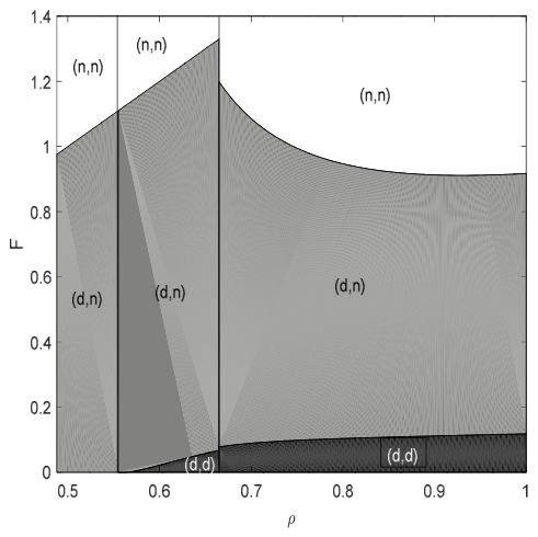
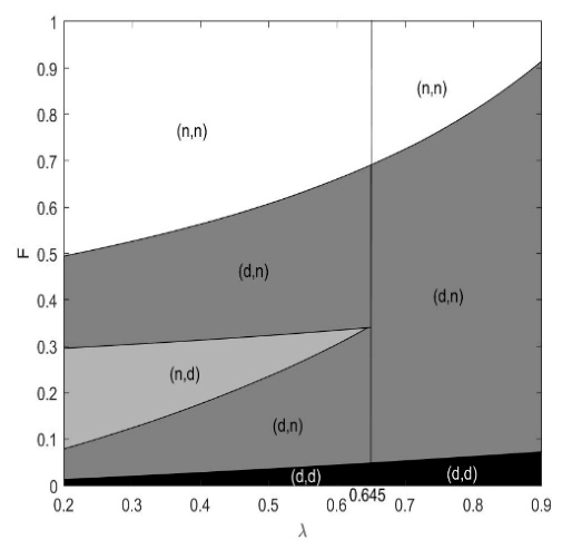
Proposition 1 shows that when the streamer’s information disclosure level is low ($\rho <{\rho }_1$), retailer 2 will always abandon disclosure regardless of the cost of disclosure. Figure 2 shows the information strategies with respect to $\rho$ and $F$ when $\tau =0.5$, $\lambda =0.9$, ${\delta }_1=1$ and ${\delta }_2=1.61$, reflecting sections (2)–(4) in Proposition 1. To ensure that $\delta ={\displaystyle \frac{{\delta }_2}{{\delta }_1}}>{\displaystyle \frac{\left(\lambda +13\tau \right)}{\left(11\tau -\lambda \right)}}$, when $\tau =0.5$, $\lambda =0.9$, ${\delta }_1=1$, it is necessary to ensure that ${\delta }_2>1.61$. Figure 3 shows the information strategies with respect to $\lambda$ and $F$ when $\tau =0.5$, $\rho =1$, ${\delta }_1=1$ and ${\delta }_2=1.61$, which verifies the conclusion that as the trust factor increases, retailer 2 will abandon the information disclosure strategy. When $0.488\le \rho <0.555$, given a fixed $\rho$, two retailers’ information disclosure policies will transform from $\left(d,n\right)$ to $\left(n,n\right)$ with the increase of $F$; when $\rho \ge 0.555$, two retailers’ information disclosure policies will transform from $\left(d,d\right)$ to $\left(d,n\right)$ and finally transform into $\left(n,n\right)$ with the increase of $F$. Actually, although the value of $\rho$ is relatively high here, it does not reach the threshold for implementing the $\left(n,d\right)$ strategy. Retailer 2 will only disclose information when the disclosure cost is low enough since once one of the competing retailers fails to disclose information, the corresponding retailer will be withdrawn from the market; retailer 1 here will also adopt to disclose information. However, retailer 2 will lose the market due to the fact that the profit gain from information disclosure cannot offset disclosure costs.

Proposition 1 shows that the equilibrium strategy differs with the change of $F$ and $\rho$. The final strategy can be divided into five sections according to the change of $\rho$, and each section is made up of different parts based on the variation of $F$. To better analyze the equilibrium strategy, we denote the strategies when retailer 2 always withholds information as $S_1$, the strategies when retailer 2 adopts the opposite information strategy as retailer 1’s strategy as $S_2$, and the strategies when retailer 2 always discloses information as $S_3$. As

Table 6. The divisions of different information strategies.

Region	$\mathit{\rho }$	$\mathit{F}$	$\mathit{S}$	${\mathit{S}}_{\mathit{i}}$
1	$\rho <{\rho }_1$	$F\in \left[0, 4\rho \tau \right)$	$\left(d,n\right)$	$S_1$
	${\rho }_1\le \rho <{\rho }_4$	$F\in [0,F_{f1})$	$\left(d,n\right)$	$S_2$
		$F\in [F_{f1},F_a)$	$\left(n,d\right)$	$S_2$
		$F\in \left[F_a,4\rho \tau \right)$	$\left(d,n\right)$	$S_1$
	${\rho }_4\le \rho <{\rho }_3$	$F\in [0,F_{f1})$	$\left(d,n\right)$	$S_2$
		$F\in [F_{f1},F_a)$	$\left(n,d\right)$	$S_2$
	${\rho }_3\le \rho <{\rho }_5$	$F\in \left[0,F_a\right)$	$\left(n,d\right)$	$S_2$
2	${\rho }_5\le \rho <{\rho }_2$	$F\in \left[0,F_a\right)$	$\left(n,d\right)$	$S_2$
		$F\in \left[F_a,4\rho \tau \right)$	$\left(d,n\right)$	$S_1$
	${\rho }_2\le \rho <{\displaystyle \frac{{(1+\lambda )}^2}{13\tau {\zeta }_1}}$	$F\in \left[0, 4\rho \tau \right)$	$\left(d,n\right)$	$S_1$
3	${\displaystyle \frac{{(1+\lambda )}^2}{13\tau {\zeta }_1}}\le \rho <{\displaystyle \frac{{\left(1+\lambda \right)}^2}{{\zeta }_1\left(13\tau -\lambda \right)}}$	$F\in \left[0, F_{b3} \right)$	$\left(d,d\right)$	$S_3$
		$F\in [F_{b3},4\rho \tau )$	$\left(d,n\right)$	$S_1$
	${\displaystyle \frac{{\left(1+\lambda \right)}^2}{{\zeta }_1\left(13\tau -\lambda \right)}}\le \rho <{\rho }^{*}$	$F\in \left[0, F_{b4} \right)$	$\left(d,d\right)$	$S_3$
		$F\in \left[F_{b4},F_{d4} \right)$	$\left(d,n\right)$	$S_1$
4	$\rho \ge {\rho }^{*}$	$F\in \left[0, F_{b4} \right)$	$\left(d,d\right)$	$S_3$
		$F\in [F_{b4},F_{f4})$	$\left(d,n\right)$	$S_2$
		$F\in [F_{f4},F_a)$	$\left(n,d\right)$	$S_2$
		$F\in \left[F_a,F_{d4}\right)$	$\left(d,n\right)$	$S_1$

shows, we further divide the whole information strategies in Proposition 1 except strategy $\left(n,n\right)$ into four regions.

In region 1, the disclosure level is so low that given a fixed low disclosure cost, retailer 2 does not have obvious willingness to disclose information, and retailer 2’s information strategy will transform from $S_1$ to $S_2$. In region 2, the disclosure level here is higher than that in region 1, and strategy $S_1$ is prone to occur; actually, one may intuitively think that $S_1$ is less likely to occur due to the fact that retailer 2 can be better off from increased $\rho$ (see Proposition 4); however, the final information strategy in equilibrium is quite the opposite. In region 2, retailer 1 will be eliminated by the market if he withholds information, consequently, retailer 1 still adopts to disclose information. Retailer 2 will passively withhold information in region 2 since the value of $\rho$ does not reach the threshold to achieve $\left(d,d\right)$ strategy. As $\rho$ further increases, strategy $S_3$ occurs in region 3 due to the fact that retailer 2 here can benefit more from disclosed information than in region 2 when the disclosure cost is low.

In a sequential information disclosure game, the first mover will make information decisions anticipating the second mover’s corresponding decisions, whereas the first mover’s strategy also affects the second mover’s strategy. Actually, a higher value of ρ means that the retailers’ signal is more accurate, and customers are clearer about the misfit; as a result, the customers’ utility becomes more heterogeneous, which softens the competition between two retailers. When the disclosure level is low enough ($\rho <{\rho }_1$), the competition between two retailers is so intense that the profit gain from more transparent information cannot make up for the disclosure cost, and retailer 2 will withhold information; retailer 2 is unable to make positive profit and finally withdraws from the market. Accordingly, retailer 1 will adopt information disclosure even though the disclosure level here is low due to the fact that if both retailers withhold information, they will all withdraw from the market. With the increase of $\rho$ ($\rho \ge {\rho }_3$), retailer 2 transacting with the supplier inefficient in product is prone to disclose information to make up for the low product quality. In Proposition 1(1), we can find that when $\rho <{\displaystyle \frac{{\left(1+\lambda \right)}^2}{\left(\lambda +13\tau \right){\zeta }_1}}$ and $F<F_a$, retailer 2 will adopt the opposite information strategy as retailer 1’s strategy in equilibrium. Retailer 1 under the condition will choose to withhold information, further leading to the phenomenon that he will withdraw from the market. As $\rho$ further increases, i.e., $\rho \ge {\displaystyle \frac{{(1+\lambda )}^2}{13\tau {\zeta }_1}}$, retailer 2 always discloses information, and retailer 1 here will also adopt information disclosure strategy. When the information disclosure level is fixed, two retailers will neither disclose information if the disclosure cost is high, and two retailers will withdraw from the marketplace due to the loss of profits.

There exists a second mover advantage in a sequential information disclosure game when ${\rho }_3\le \rho <{\displaystyle \frac{{(1+\lambda )}^2}{(\lambda +13\tau ){\zeta }_1}}$ and $F<F_a$ or when ${\rho }_1\le \rho <{\rho }_4$ and $F\in [F_{f1},F_a)$ due to the fact that if retailer 1 here also adopts information disclosure, he will obtain the positive profit, which can be denoted by $4\rho \tau -F$. However, in the equilibrium information disclosure decision, retailer 1 ultimately gives up disclosure and withdraws from the market.

Proposition 2.

When incorporating the effects of trust into the customers’ utility, it increases the possibility for two retailers to disclose information simultaneously.

When neglecting the effects of trust on the customers’ utility, namely, $\lambda =0$, the proof in Appendix A shows that strategies $\left(d,n\right)$, $\left(n,d\right)$, and $\left(n,n\right)$ still exist under some conditions, whereas strategy $\left(d,d\right)$ will never exist. When considering the effects of information disclosure on the customers’ trust, it homogenizes customers’ perceived utility differences, and the trust factor intensifies the competition between two retailers. This phenomenon can also be illustrated by the demand function ${\displaystyle \frac{\rho \tau -p_{1dd}+p_{2dd}+(1+\lambda ){(Z}_{1dd}-Z_{2dd})}{2\rho \tau }}$; when $\lambda =0$, the coefficient representing the quality substitutability can be denoted by ${\displaystyle \frac{1}{2\rho \tau }}$, and when $\lambda \ne 0$, the corresponding coefficient increases to ${\displaystyle \frac{1+\lambda }{2\rho \tau }}$, which confirms the increasing competition caused by the trust factor. When tracing back to the customers’ utility function, the trust-related utility $(\rho +Z_{1dd})\lambda$ reduces the heterogeneity in the customers’ perceived utility; thus, the increased competition between two products incurs two retailers to disclose information.

5.2. Information Strategies Considering Different Market Coverage

In this section, we begin by examining the information strategies of the two retailers under full, partial, and no coverage scenarios; then, we further obtain Proposition 3, which shows the relationship between information disclosure and market coverage.

Proposition 3.

Two retailers’ information strategies considering different market coverages are shown in

Table 7. Information strategies in the scenario of full coverage.

Information Strategies	$\mathit{\rho }$	$\mathit{F}$
$\left(d,d\right)$	${\displaystyle \frac{{(1+\lambda )}^2}{13\tau {\zeta }_1}}\le \rho <{\displaystyle \frac{{\left(1+\lambda \right)}^2}{{\zeta }_1\left(13\tau -\lambda \right)}}$	$F\in [0,F_{b3})$
$\left(d,d\right)$	${\displaystyle \frac{{\left(1+\lambda \right)}^2}{{\zeta }_1\left(13\tau -\lambda \right)}}\le \rho <{\rho }^{*}$	$F\in [0,F_{b4})$
$\left(d,n\right)$	${\displaystyle \frac{{\left(1+\lambda \right)}^2}{{\zeta }_1\left(13\tau -\lambda \right)}}\le \rho <{\rho }^{*}$	$F\in [F_{b4},F_{d4})$
$\left(d,d\right)$	$\rho \ge {\rho }^{*}$	$F\in [0,F_{b4})$
$\left(d,n\right)$	$\rho \ge {\rho }^{*}$	$F\in [F_{b4},F_{f4})$
$\left(n,d\right)$	$\rho \ge {\rho }^{*}$	$F\in [F_{f4},F_a)$
$\left(d,n\right)$	$\rho \ge {\rho }^{*}$	$F\in [F_a,F_{d4})$

,

Table 8. Information strategies in the scenario of partial coverage.

Information Strategies	$\mathit{\rho }$	$\mathit{F}$
$\left(d,n\right)$	$\rho <{\rho }_1$	$F<4\rho \tau$
$\left(d,n\right)$	${\rho }_1\le \rho <{\rho }_4$	$F<F_{f1}$
$\left(n,d\right)$	${\rho }_1\le \rho <{\rho }_4$	$F_{f1}\le F<F_a$
$\left(d,n\right)$	${\rho }_1\le \rho <{\rho }_4$	$F_a\le F<4\rho \tau$
$\left(d,n\right)$	${\rho }_4\le \rho <{\rho }_3$	$F<F_{f1}$
$\left(n,d\right)$	${\rho }_4\le \rho <{\rho }_3$	$F_{f1}\le F<F_a$
$\left(n,d\right)$	${\rho }_3\le \rho <{\rho }_2$	$F<F_a$
$\left(d,n\right)$	${\rho }_5\le \rho <{\rho }_2$	$F_a\le F<4\rho \tau$
$\left(d,n\right)$	${\rho }_2\le \rho <{\displaystyle \frac{{\left(1+\lambda \right)}^2}{13\tau {\zeta }_1}}$	$F<4\rho \tau$
$\left(d,n\right)$	${\displaystyle \frac{{\left(1+\lambda \right)}^2}{13\tau {\zeta }_1}}\le \rho <{\displaystyle \frac{{\left(1+\lambda \right)}^2}{(13\tau {-\lambda )\zeta }_1}}$	$F_{b3}\le F<4\rho \tau$

and

Table 9. The optimal decisions with respect to $\rho$ and $\lambda$.

$\left(d,d\right)$

$Z_1$

$Z_2$

$l_1$

$l_2$

$p_1$

$p_2$

$D_1$

$D_2$

${\pi }_{r1}$

${\pi }_{r2}$

${\pi }_{l1}$

${\pi }_{l2}$

$\rho \uparrow$

$\downarrow$

$\uparrow$

$\downarrow (\rho <{\rho }_7^{*})$

$\uparrow$

$\downarrow (\rho <{\rho }_8^{*})$

$\uparrow$

$\downarrow$

$\uparrow$

$\downarrow (\rho <{\rho }_9^{*})$

$\uparrow$

$\uparrow ({\displaystyle \frac{104}{49}}<{\displaystyle \frac{{\zeta }_2}{{\zeta }_1}})$

$\uparrow$

$\uparrow (\rho >{\rho }_7^{*})$

$\uparrow (\rho >{\rho }_8^{*})$

$\uparrow (\rho >{\rho }_9^{*})$

$\lambda \uparrow$

$\uparrow$

$\downarrow (\rho <{\rho }_6^{*})$

$\uparrow$

$\downarrow$

$\uparrow$

$\downarrow$

$\uparrow$

$\downarrow$

$\uparrow$

$\downarrow$

$\downarrow$

$\uparrow (\rho >{\rho }_6^{*})$

.

The market coverage under different information strategies is determined by the disclosure cost $F$ and the level of disclosed information $\rho$. When the disclosure level is low enough ($\rho <{\displaystyle \frac{{(1+\lambda )}^2}{13\tau {\zeta }_1}}$), the market cannot be fully covered regardless of the size of $F$, which confirms that the low disclosure level increases the competition between two retailers; retailer 2 under this condition will withdraw from the market due to the high competition. In the scenario of partial coverage, the retailer without information disclosure will lose the market. When the disclosure cost is quite high, two retailers both withhold information, two retailers will lose the market, and the market coverage will be 0. Interestingly, although Table 4 shows that when two retailers both disclose information, retailer 2 will still withdraw from the market due the low profit from disclosure when the disclosure level is low ($\rho <{\displaystyle \frac{{(1+\lambda )}^2}{13{\zeta }_1\tau }}$). However, Proposition 1 shows that strategy $\left(d,d\right)$ in equilibrium will never occur when $\rho <{\displaystyle \frac{{(1+\lambda )}^2}{13{\zeta }_1\tau }}$, which indicates that the market will be fully covered once two retailers adopt to disclose information regardless of the disclosure level. Table 8 shows that when the disclosure level is low ($\rho <min({\displaystyle \frac{{(1+\lambda )}^2}{{\zeta }_1(13\tau -\lambda )}},{\displaystyle \frac{{(1+\lambda )}^2}{(\lambda +13\tau ){\zeta }_1}})$), information disclosure can effectively affect the market share, and the retailer who withholds information will withdraw from the marketplace due to the intense competition.

Proposition 4.

When two retailers both disclose information, the optimal decisions with respect to $\rho$ and $\lambda$ are presented in Table 9, where $\uparrow$ and $\downarrow$ represent increase and decrease, respectively.

Proposition 4 demonstrates that an increased value of $\lambda$ intensifies competition by rendering customers’ utility homogeneous, and a higher value of $\rho$ makes the customers’ valuations about the products heterogeneous and hence softens the competition. When tracing back to the demand function, we can find that both the price competition and quality competition exist in the market, ${\displaystyle \frac{1}{2\rho \tau }}$ measures the price sensitivity coefficients and price substitutability between the two products, and ${\displaystyle \frac{1+\lambda }{2\rho \tau }}$ measures the quality sensitivity coefficients and quality substitutability between the two products. As $\rho$ increases, both the price and quality substitutability between the two products decrease, which leads to the decreased price competition and quality competition between two products. However, when $\rho$ increases, the price and quality sensitivity coefficients will also decrease, which means that the customers will be less sensitive to the price and product quality. As $\lambda$ increases, the quality sensitivity coefficients and quality substitutability between the two products will be higher, which means that the customers are more sensitive to quality, and the quality competition between two products will be fiercer. Although both the product quality and information transparency can affect product trust, when two retailers both disclose information, the effect of information transparency on product trust will be offset, which highlights the importance of quality on the demand by increasing customers’ trust. Since supplier 1 is more efficient in quality investment than supplier 2, supplier 1 can benefit from the increased trust factor by improving quality investments and increasing wholesale prices. However, supplier 2 will hurt from the increased trust factor. The same reason can be applied to analyze the effects of $\rho$ on supplier 2’s profit. Supplier 2 is insufficient in quality investment; thus, he can benefit from the decreased competition, and decreased price and quality sensitivity, as $\rho$ increases. The effects of $\rho$ on supplier 1’s profit are complex. On one hand, the decreased competition and customers’ quality sensitivity caused by the higher information transparency are detrimental for supplier 1 to leverage her advantage of quality investment. On the other hand, the customers will be less sensitive to the price as $\rho$ increases; thus, supplier 1 can set a higher price to obtain more profits. Supplier 1 will obtain more or fewer profits, which depends on the trade-off between the above two effects. A higher value of $\lambda$ incentives supplier 1 to increase quality investments, which allows retailer 1 to set a higher retail price for product 1 and makes retailer 1 better off.

Transparent supply chains can reduce reputational risk and gain customer trust for the enterprise (https://hbr.org/2019/08/what-supply-chain-transparency-really-means accessed on 26 July 2026). This paper suggests that the retailer transacting business with the supplier inefficient in products discloses information. When two retailers both disclose information, the market is fully covered. Retailers’ information disclosure has dual effects on the customers’ trust; one effect is the direct effect that the information transparency can affect customers’ trust, which can be shown from $\rho \lambda$ in the utility function. The other is an indirect effect, which can be shown in $q\lambda$ in the utility function due to the fact that $q$ can be affected by $\rho$. Although when two retailers both disclose information, the direct effects of information disclosure on customers’ trust can be offset; more transparent information will improve the suppliers’ products, which indirectly increases customer trust, making the retailer better off with the increase of information transparency.

Proposition 5.

When two retailers both disclose information, the decisions satisfy the following conditions:

• (1) $Z_{1dd}>Z_{2dd}$; $p_{1dd}>p_{2dd}$; $l_{1dd}\ge l_{2dd}$ if $\rho \le {\displaystyle \frac{{(1+\lambda )}^2({\zeta }_2-{\zeta }_1)}{2\tau {\zeta }_1{\zeta }_2}}$, else, $l_{1dd}<l_{2dd}$;
• (2) $D_{1dd}\ge D_{2dd}$ if $\rho \le {\displaystyle \frac{{\left(1+\lambda \right)}^2(\zeta -1)}{2\tau {\zeta }_2}}$, else, $D_{1dd}<D_{2dd}$;
• (3) ${\pi }_{r1dd}>{\pi }_{r2dd}$.

Proposition 4 has shown the effects of $\rho$ on the price or quality competition and on the price and quality sensitivity coefficients. When two retailers both disclose information, if the level of disclosure is relatively high, retailer 2 can gain more market share through information disclosure. The above phenomenon shows that retailer 2 can gain more advantages in market share through information disclosure when the level of information disclosure is relatively high. When two retailers both disclose information, supplier 1 will provide higher-quality investments; interestingly, the corresponding wholesale price of supplier 1 is not always higher than that of supplier 2. The reasons can be explained as follows: Supplier 1 is incentivized to enhance quality because of its high efficiency, prompting retailer 1 to charge a higher sales price. However, as $\rho$ increases, the adverse impact of the higher sales price on demand outweighs the benefits of improved quality. Consequently, retailer 1’s sales volume may fall below that of retailer 2 when $\rho >{\displaystyle \frac{\left(1+\lambda {)}^2(\zeta -1\right)}{2\tau {\zeta }_2}}$. To keep the balance, supplier 1 as the leader in the whole game will adjust the demand allocation by reducing the wholesale price.

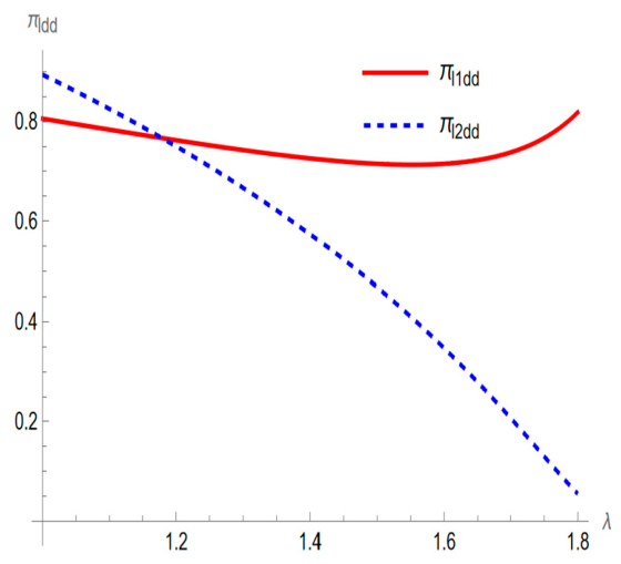
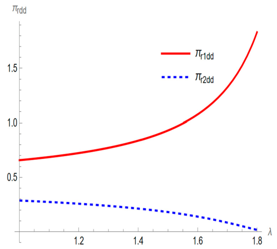
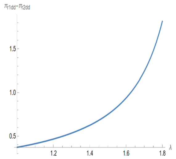
To better analyze the effects of $\lambda$ on the retailers’ profits under strategy $\left(d,d\right)$, we assume that $\rho =0.7$, $\tau =0.9$, ${\delta }_1=1$, ${\delta }_2=1.61$, $F=0.01$. To ensure that $\delta ={\displaystyle \frac{{\delta }_2}{{\delta }_1}}>{\displaystyle \frac{\left(\lambda +13\tau \right)}{\left(11\tau -\lambda \right)}}$, when $\rho =0.7$, $\tau =0.9$, ${\delta }_1=1$, it is necessary to ensure that ${\delta }_2>{\displaystyle \frac{\lambda +11.7}{9.9-\lambda }}$; which shows that as $\lambda$ increases, ${\delta }_2$ also increases accordingly. As shown in Figure 4, as $\lambda$ increases, retailer 1’s profit increases, and retailer 2’s profit decreases. In Figure 4, ${\pi }_{r1dd}-{\pi }_{r2dd}$ is always more than 0 and increases with $\lambda$, indicating that retailer 1 can increase the profit gap with retailer 2 with the increase of $\lambda$. Figure 4 and Figure 5 mean that a higher value of $\lambda$ can make retailer 1 better off due to the increased customers’ quality sensitivity and fiercer quality competition between two products.

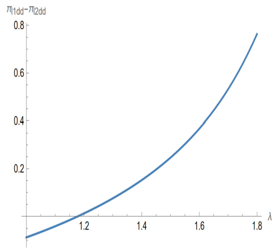
Figure 6 illustrates the impact of $\lambda$ on suppliers’ profits, revealing that supplier 1’s profit first decreases and then increases with $\lambda$; supplier 2’s profit always decreases with $\lambda$. Figure 7 reflects that supplier 1 sometimes can be worse than supplier 2, and supplier 1 can be better off with the increase of $\lambda$. As $\lambda$ increases, both the quality investments and the customers’ demand increase. For supplier 1, the profit gain from the increased demand outweighs the profit loss from increased quality investment costs when $\lambda$ is less than a certain threshold, and then supplier 1’s profit increases with $\lambda$ as $\lambda$ is higher than the threshold.

To better analyze the effects of $\rho$ on the suppliers’ or the retailers’ profits, we assume that $\lambda =0.9$, $\tau =0.9$, ${\delta }_1=1$, ${\delta }_2=1.61$, $F=0.01$. To ensure that $\delta ={\displaystyle \frac{{\delta }_2}{{\delta }_1}}>{\displaystyle \frac{\left(\lambda +13\tau \right)}{\left(11\tau -\lambda \right)}}$, when $\lambda =0.9$, $\tau =0.9$, ${\delta }_1=1$, it is necessary to ensure that ${\delta }_2>1.4$.

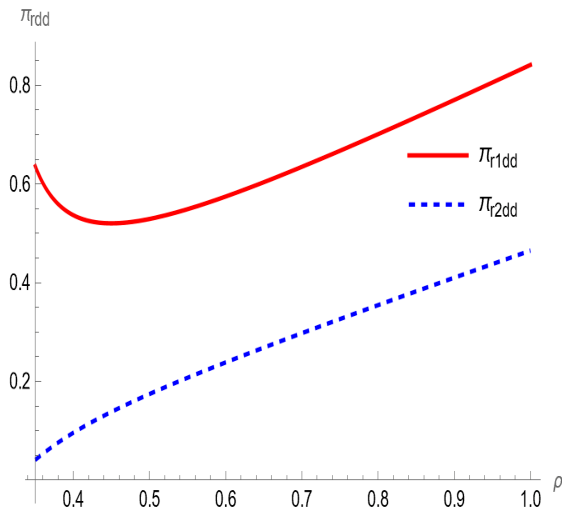
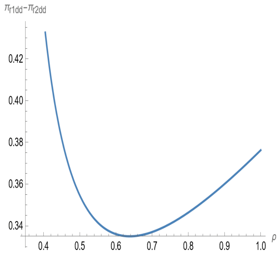
Figure 8 confirms the conclusions in Proposition 4, that is, retailer 1’s profit first decreases with $\rho$ and then increases with $\rho$, retailer 2’s profit consistently increases as $\rho$ grows. Figure 8 and Figure 9 shows that retailer 2 can narrow the profit gap with retailer 1 as $\rho$ increases when $\rho$ is low.

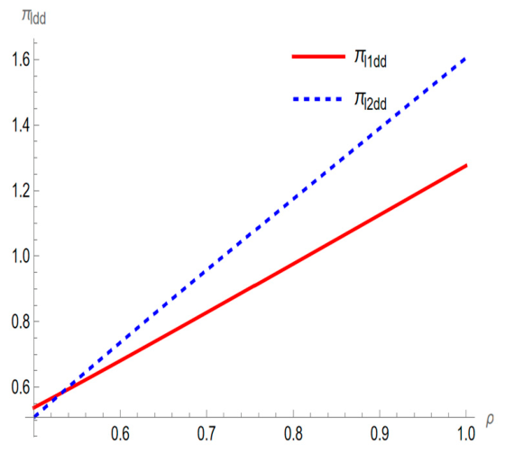
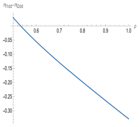
As shown in Figure 10 and Figure 11, the two suppliers’ profits increase as $\rho$ increases, whereas supplier 2 can benefit more from increased $\rho$; thus, the profit gap between two suppliers decreases, and sometimes supplier 2 can obtain more profits than supplier 1. As Figure 4, Figure 5, Figure 6, Figure 7, Figure 8, Figure 9, Figure 10 and Figure 11 show, the effects of $\rho$ and $\lambda$ on the optimal decisions show the opposite trends, that is, $∆{\pi }_r$ and $∆{\pi }_l$ decrease as $\rho$ increases, and $∆{\pi }_r$ and $∆{\pi }_l$ increase as $\lambda$ increases. Proposition 4(4) shows that the demand of product 1 decreases with $\rho$, whereas that of product 2 increases with $\rho$ and finally leads to the phenomenon shown in Proposition 5(2) that the demand of product 2 can be higher than that of product 1 when $\rho >{\displaystyle \frac{{\left(1+\lambda \right)}^2(\zeta -1)}{2\tau {\zeta }_2}}$; meanwhile, the quality investment of two suppliers shows the same trends as demand with the increase of $\rho$. The above two forces incur supplier 2 to benefit more from increased information transparency than supplier 1.

Proposition 6.

When the market is fully covered by two retailers, given the other retailer’s information strategies,

• (1) one retailer’s information disclosure affects one’s own decision-making as follows:
• it improves the product quality and increases corresponding sales and product prices.
• (2) one retailer’s information disclosure affects the other’s decision-making following the opposite trends.

To find the effects of one retailer’s information disclosure on one’s own decision-making, we compare retailer 2’s demand functions outlined in Equations (1) and (3) and find that the potential market size shifts from product 1 to product 2 due to retailer 2’s information disclosure. As a result, the product quality and product trust are improved, and the corresponding sales and product prices are increased. The same trends are shown in retailer 1’s demand functions outlined in Equations (3) and (5). We compare retailer 1’s demand functions outlined in Equations (1) and (3) and retailer 2’s demand functions outlined in Equations (3) and (5) and then can obtain Proposition 5(2).

6. Conclusions and Managerial Implications

Product quality and corresponding information transparency affect customers’ trust in products and further affect customers’ willingness to pay. Suppliers invest in quality investment to improve product quality to stimulate demand. On the other hand, green products are typically trust-based goods, and consumers often find it challenging to verify the authenticity of a product’s green attributes, even after purchasing and using it. The characteristics of green products create information asymmetry between supply and demand, leading customers to develop subjective perceptions of product quality, and the customers’ preferences for green attributes are heterogeneous. Recently, more and more retailers such as JD Qixian and Carrefour use traceability systems to disclose product information.

This paper constructs the model where two competitive retailers sell products with uncertain green information to customers, and two suppliers invest in technologies to stimulate demand through improved product quality. Both the product quality and the information transparency can affect the customers’ trust, which further affects the customers’ willingness to pay, and the retailers can determine whether to adopt information disclosure strategies or not based on profit comparison before and after information disclosure. We find that there exists a second mover advantage in a sequential information disclosure game. A higher trust factor enhances the intensity of competition by making customers’ utility homogeneous, whereas higher information transparency makes the customers’ valuations about the products heterogeneous and hence softens the competition. This paper suggests the retailer transacting business with the supplier inefficient in products discloses information, whereas the fiercer quality competition from increased trust factor has a detrimental effect on the supplier with low product efficiency. Retailer 2 can gain more advantages in market share through information disclosure when the level of information disclosure is relatively high in the information strategy $\left(d,d\right)$.

The management implications of this article are as follows. Retailers who deal with low-quality investment efficiency suppliers should proactively disclose information if the information transparency level is high because transparency can avoid being completely eliminated by the market due to quality shortcomings. When consumers’ overall trust in green products increases, it will intensify positive competition among retailers, which results in suppliers with low-quality investment efficiency suffering more severe losses in competition.

This article requires further research on the following aspects. The sequence of information disclosure may affect the decisions; in this paper, we assume that two retailers disclose information sequentially, and a comparison of simultaneous disclosure and sequential disclosure needs to be further studied. However, to highlight the effects of the difference in products on the decisions, this paper avoids comparison of complex information disclosure decisions. Meanwhile, this paper only considers two competing supply chains with complete information. Future studies could extend the proposed framework by incorporating multiple competing agents, stochastic demand, behavioral consumer heterogeneity, dynamic game-theoretic settings, or empirical validation of the analytical results.

References

1. Moon, J.; Song, M.; Lee, W.S.; Shim, J. Structural relationship between product quality, usefulness, ease of use, convenience, brand trust and willingness to pay: The case of Starbucks. Br. Food J. 2023, 125, 65–81. [Google Scholar]
2. Fu, S.L.; Liu, X.D.; Abdesslam, L.; Liu, H.; Huang, Y.T. Green production information transparency and online purchase behavior: Evidence from green agricultural products in China. Front. Environ. Sci. 2022, 10, 985101. [Google Scholar] [CrossRef]
3. Fu, S.L.; Hu, X.X.; Zhang, C.; Li, Z.P. A study on the influence of production and environmental information transparency on online consumers’ purchase intention of green agricultural products. Br. Food J. 2025, 127, 1461–1479. [Google Scholar] [CrossRef]
4. Zhang, W.; Wang, S.; Wan, L.; Zhang, Z.; Zhao, D. Information perspective for understanding customers’ perceptions of electric vehicles and adoption intentions. Transp. Res. Part D Transp. Environ. 2022, 102, 103157. [Google Scholar] [CrossRef]
5. He, Y.; He, D.X.; Xu, Q.Y. Optimal product line design strategy for green and non-green products with blockchain technology. Ann. Oper. Res. 2026, 359, 1697–1726. [Google Scholar]
6. Niu, B.; Xu, H.; Chen, L. Creating all-win by blockchain in a remanufacturing supply chain with customer risk-aversion and quality untrust. Transp. Res. Part E Logist. Transp. Rev. 2022, 163, 102778. [Google Scholar] [CrossRef]
7. Lv, Y.; Bi, X.H. How blockchain technology combats greenwashing: A game in a low-carbon preference market. Comput. Ind. Eng. 2025, 209, 111562. [Google Scholar] [CrossRef]
8. Ma, S.G.; He, Y. Investment of green technology in a tourism supply chain under competition. IEEE Trans. Eng. Manag. 2023, 70, 1199–1214. [Google Scholar] [CrossRef]
9. Zhang, X.X.; Jin, Y.N.; Shen, C.L. Manufacturers’ green investment in a competitive market with a common retailer. J. Clean. Prod. 2020, 276, 123164. [Google Scholar] [CrossRef]
10. Zhang, X.X.; Chen, T.; Shen, C.L. Green investment choice in a duopoly market with quality competition. J. Clean. Prod. 2020, 276, 124032. [Google Scholar] [CrossRef]
11. Yang, S.X.; Ding, P.Q.; Wang, G.; Wu, X.L. Green investment in a supply chain based on price and quality competition. Soft Comput. 2020, 24, 2589–2608. [Google Scholar]
12. Hafezi, M.; Zhao, X.; Zolfagharinia, H. Together we stand? Co-opetition for the development of green products. Eur. J. Oper. Res. 2023, 306, 1417–1438. [Google Scholar] [CrossRef]
13. Adnan, Z.H.; Chakraborty, K.; Bag, S.; Wu, J.S. Pricing and green investment strategies for electric vehicle supply chain in a competitive market under different channel leadership. Ann. Oper. Res. 2025, 355, 87–122. [Google Scholar]
14. Li, J.; Liang, J.; Shi, V.; Zhu, J. The benefit of manufacturer encroachment considering consumer’s environmental awareness and product competition. Ann. Oper. Res. 2025, 349, 1087–1107. [Google Scholar]
15. Zong, S.L.; Zhang, L.B.; Lei, R.X. Product line strategy for green and non-green products in hybrid platform retailing. Ann. Oper. Res. 2025, 346, 2349–2385. [Google Scholar] [CrossRef]
16. Zhang, L.B.; Zong, S.L.; Lei, R.; Wang, W.T. Green or nongreen? Product line design for competing manufacturers in a platform supply chain. Comput. Ind. Eng. 2026, 211, 111614. [Google Scholar] [CrossRef]
17. Zhang, L.; Shao, Z.; Zhao, T.; Li, X.T.; Zhang, J.F. Digitally-enabled antecedents of trust, repurchase intention and the impact of blockchain traceability labels. Electron. Commer. Res. Appl. 2024, 68, 101469. [Google Scholar] [CrossRef]
18. Cai, J.H.; Sun, H.N.; Shang, J.; Hegde, G.G. Information structure selection in a green supply chain: Impacts of wholesale price and greenness level. Eur. J. Oper. Res. 2023, 306, 34–46. [Google Scholar] [CrossRef]
19. Ma, X.; Xu, J.; Peng, W.; Wang, S. Optimal freshness and carbon abatement decisions in a two-echelon cold chain. Appl. Math. Model. 2021, 96, 834–859. [Google Scholar] [CrossRef]
20. Chen, Q.; Duan, Y.R. Impact of information disclosure on global supply chain greenwashing: Is more information transparency always better? Transp. Res. Part E Logist. Transp. Rev. 2023, 178, 103288. [Google Scholar] [CrossRef]
21. Hong, X.P.; Cao, X.L.; Gong, Y.; Chen, W.Y. Quality information acquisition and disclosure with green manufacturing in a closed-loop supply chain. Int. J. Prod. Econ. 2021, 232, 107997. [Google Scholar] [CrossRef]
22. Wang, L.K.; Li, M.; Wang, W.; Gong, Y.; Xiong, Y. Green innovation output in the supply chain network with environmental information disclosure: An empirical analysis of Chinese listed firms. Int. J. Prod. Econ. 2023, 256, 108745. [Google Scholar] [CrossRef]
23. Li, Y.J.; Yao, S.; Wang, J. Signaling strategies in a low-carbon supply chain with platform encroachment. Transp. Res. Part E Logist. Transp. Rev. 2023, 179, 103319. [Google Scholar] [CrossRef]
24. Zhou, Y.; Yan, S.Q.; Li, G.; Xiong, Y.; Lin, Z.B. The impact of consumer skepticism on blockchain-enabled sustainability disclosure in a supply chain. Transp. Res. Part E Logist. Transp. Rev. 2023, 179, 103323. [Google Scholar] [CrossRef]
25. Hsieh, C.C.; Wu, C.Y.; Lathifah, A. Cross-channel influence of blockchain technology on green supply chains under asymmetric retail platform competition. Int. J. Prod. Econ. 2025, 283, 109584. [Google Scholar] [CrossRef]
26. Guo, S.; Sun, X.T.; Lam, H.K.S. Applications of blockchain technology in sustainable fashion supply chains: Operational transparency and environmental efforts. IEEE Trans. Eng. Manag. 2023, 70, 1312–1328. [Google Scholar] [CrossRef]
27. Yao, Y.F.; Liu, T.T.; Tian, G.X. Improve the sustainability of supply chain: The role of carbon abatement and blockchain technology. RAIRO-Oper. Res. 2025, 59, 115–148. [Google Scholar] [CrossRef]
28. Srisathan, W.A.; Naruetharadhol, P. Exploring moral hazard and adverse selection in the context of greenwashing and organic product consumption. J. Retail. Consum. Serv. 2025, 84, 104203. [Google Scholar] [CrossRef]
29. Liu, H.; Ma, R.L.; He, G.; Fu, S.L. The impact of blockchain technology on the online purchase behavior of green agricultural products. J. Retail. Consum. Serv. 2023, 74, 103387. [Google Scholar] [CrossRef]
30. Duong, C.D.; Nguyen, T.H.; Nga, N.T.V.; Bui, T.V.; Tran, N.M. Perceived blockchain-related information transparency and organic food purchase intention: An extension of the theory of planned behaviour with the moderation role of blockchain-based trust. Br. Food J. 2025, 127, 1131–1152. [Google Scholar] [CrossRef]
31. Zhang, K.R.; Li, X.Y.; Bai, Y. When green meets economic: Blockchain adoption, channel conflict, and sustainable remanufacturing strategies. Int. J. Ind. Eng. Comput. 2026, 17, 785–804. [Google Scholar] [CrossRef]
32. Liu, H.; Zhang, W.K.; Huang, Y.T. Exploring the mechanism of blockchain technology application on consumers’ green agricultural product purchasing behavior: A qualitative study. J. Consum. Prot. Food Saf. 2025, 20, 225–233. [Google Scholar] [CrossRef]
33. Tao, Z.B.; Chao, J.X. The impact of a blockchain-based food traceability system on the online purchase intention of organic agricultural products. Innov. Food Sci. Emerg. Technol. 2024, 92, 103598. [Google Scholar] [CrossRef]
34. Cheng, M.Y.; Chong, H.Y.; Xu, Y.; Wu, H.T. Fostering green building project performance by blockchain-enabled smart contracts (B-SCs) implementation: Adaptive structuration perspective. J. Build. Eng. 2025, 114, 114435. [Google Scholar] [CrossRef]
35. He, L.F.; Bai, W.F.; Liu, F.T.; Yue, X.H. Blockchain technology implementation and sustainable operations in platform supply chains across diverse channel modes. Omega-Int. J. Manag. Sci. 2026, 138, 103394. [Google Scholar] [CrossRef]
36. Deng, L.R.; Zhang, Y.; Tang, L. Research on low-carbon dual-channel supply chain emission reduction and financing strategy based on blockchain. IEEE Access 2024, 12, 97115–97131. [Google Scholar] [CrossRef]
37. Lu, Q.H.; Liao, C.H.; Shi, V.; Xu, Z.P. Implementation mode selection for blockchain technology in green product traceability. Int. J. Prod. Econ. 2024, 276, 109372. [Google Scholar] [CrossRef]
38. Gu, Y.M.; Wang, W.Z.; Loh, H.S. Blockchain’s role in low-carbon supply chain decisions with game model insights. J. Clean. Prod. 2025, 502, 145356. [Google Scholar] [CrossRef]
39. Wang, X.; Li, D. A dynamic product quality evaluation based pricing model for perishable food supply chains. Omega-Int. J. Manag. Sci. 2012, 40, 906–917. [Google Scholar] [CrossRef]
40. Liu, M.; Dan, B.; Zhang, S.; Ma, S. Information sharing in an E-tailing supply chain for fresh produce with freshness-keeping effort and value-added service. Eur. J. Oper. Res. 2021, 290, 572–584. [Google Scholar] [CrossRef]
41. Chen, Z.; Wu, S.; Govindan, K.; Wang, X.-J.; Chin, K.-S.; Martíınez, L. Optimal pricing decision in a multi-channel supply chain with a revenue-sharing contract. Ann. Oper. Res. 2022, 318, 67–102. [Google Scholar] [CrossRef]
42. Li, L.J.; He, L.; Gooi, L.M.; Chong, K.M. Trust to repurchase: Investigating consumer behaviour with SOR theory and dual-stage SEM-ANN analysis. Asia Pac. J. Mark. Logist. 2026, 38, 2280–2294. [Google Scholar] [CrossRef]
43. Jia, M.J. The impacts of positive and negative product information disclosure at trade shows. J. Bus. Ind. Mark. 2026, 41, 1221–1233. [Google Scholar] [CrossRef]
44. Zhang, T.; Li, G.; Lai, K.K.; Leung, J.W.K. Information disclosure strategies for the intermediary and competitive sellers. Eur. J. Oper. Res. 2018, 271, 1156–1173. [Google Scholar] [CrossRef]
45. Sui, R.; Liu, M.; Liu, Y.; Zha, X. Two-sided dynamic pricing and value-added service investment strategies of competitive platforms considering indirect network effects. Int. J. Prod. Econ. 2024, 272, 109262. [Google Scholar] [CrossRef]
46. Lv, H.; Li, D. Impacts of heterogeneous green consumers on green innovation in electric vehicle and charging pile firms. Sustain. Prod. Consum. 2021, 28, 1216–1231. [Google Scholar] [CrossRef]
47. Kwark, Y.; Chen, J.; Raghunathan, S. Online product reviews: Implications for retailers and competing manufacturers. Inf. Syst. Res. 2014, 25, 93–110. [Google Scholar] [CrossRef]
Figure 1. The sequence of events in the game.
Mathematics 14 02833 g001
Figure 2. Information strategies with respect to ρ and F .
Mathematics 14 02833 g002
Figure 3. Information strategies with respect to λ and F .
Mathematics 14 02833 g003
Figure 4. The retailers’ profit with respect to λ .
Mathematics 14 02833 g004
Figure 5. The retailers’ profit gap with respect to λ .
Mathematics 14 02833 g005
Figure 6. The suppliers’ profit with respect to λ .
Mathematics 14 02833 g006
Figure 7. The suppliers’ profit gap with respect to λ .
Mathematics 14 02833 g007
Figure 8. The retailers’ profit with respect to ρ .
Mathematics 14 02833 g008
Figure 9. The retailers’ profit gap with respect to ρ .
Mathematics 14 02833 g009
Figure 10. The suppliers’ profit with respect to ρ .
Mathematics 14 02833 g010
Figure 11. The suppliers’ profit gap with respect to ρ .
Mathematics 14 02833 g011