Predictive Hybrid Energy Management for DC Microgrids: Adaptive Fuzzy Sliding Mode Control with Augmented Deep Q-Learning

Abstract

This paper addresses the voltage regulation problem for DC microgrids modeled as nonlinear dynamical systems subject to parametric uncertainties and external disturbances. A data-driven predictive hybrid control scheme is developed, combining a nonlinear sliding mode law that guarantees finite-time current convergence, an adaptive fuzzy universal approximator that compensates for unknown residual dynamics and mitigates chattering, and a recursive predictor built online via forgetting-factor recursive least squares. Real-time gain optimization is achieved through the minimization of a quadratic predictive performance index. A composite Lyapunov analysis rigorously establishes uniform ultimate boundedness of the low level Adaptive Fuzzy Sliding Mode Control (AFSMC) inner loop, assuming bounded reference currents provided by the DQL agent and characterizes the convergence residual set of the tracking error. Comparative simulations against conventional fuzzy logic and a standard (non augmented) Deep Q-Learning baseline with fixed gain SMC corroborate the theoretical guarantees, demonstrating superior voltage regulation, reduced battery deep discharges, and improved load management.

1. Introduction

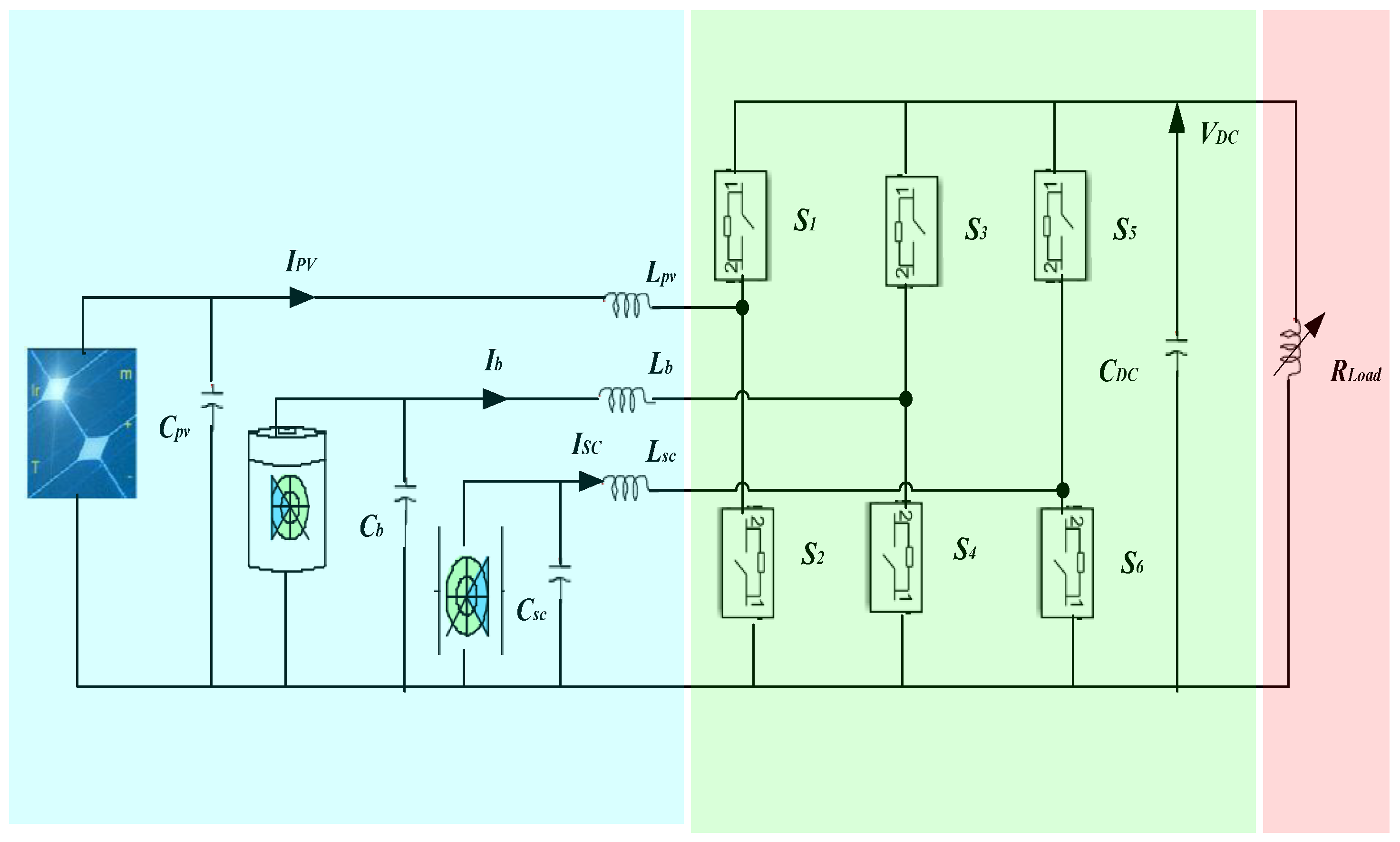
The increasing penetration of renewable energy sources and the growing demand for reliable off-grid power supply have placed direct current microgrids (DCMGs) at the forefront of modern power systems [1,2]. DCMGs offer inherent advantages such as higher efficiency, simpler integration of storage devices, and absence of reactive power and synchronization issues compared to AC microgrids [3,4]. A typical DCMG comprises photovoltaic (PV) panels, battery energy storage, supercapacitors (SCs), and variable loads, all interconnected through DC-DC converters [5]. However, the intermittent nature of solar generation and the stochastic behavior of load demand introduce significant challenges in maintaining DC bus voltage stability and ensuring optimal power sharing among storage units [6,7].

To address these challenges, various control strategies have been proposed. Linear controllers such as proportional-integral (PI) regulators are widely adopted due to their simplicity, but they often fail under large disturbances or parameter variations [8]. Nonlinear SMC has emerged as a robust alternative, offering finite-time convergence and insensitivity to matched uncertainties [9,10]. In the context of DCMGs, SMC has been successfully applied to regulate converter currents and bus voltage [11,12]. Nevertheless, classical SMC relies on fixed gains and may exhibit chattering, which can degrade actuator lifetime. Moreover, the absence of adaptation mechanisms limits its performance under rapidly changing operating conditions.

To overcome the limitations of fixed-gain controllers, fuzzy logic systems (FLS) have been integrated into adaptive control strategies. FLS can approximate unknown nonlinear functions using linguistic rules, thereby reducing the need for accurate system models [13,14]. For instance, a hierarchical energy management system combining SMC with fuzzy logic was proposed for a DCMG, achieving improved dynamic response compared to linear controllers [15]. However, fuzzy-based strategies remain heuristic and lack learning capabilities; their performance heavily depends on the quality of predefined rule bases, which may not cover extreme or unforeseen scenarios [16].

Recent advances in adaptive fuzzy control have addressed challenging issues such as event-triggered mechanisms, dynamic quantization, and deception attacks in networked control systems [17,18]. For instance, adaptive event-triggered tracking control strategies have been developed for nonlinear networked systems with dynamic quantization and deception attacks [17], while quantized fuzzy guaranteed cost control has been proposed for electric vehicles with uncertain parameters [18]. These techniques provide valuable insights for enhancing robustness and communication efficiency in complex control systems.

More recently, artificial intelligence techniques, particularly deep reinforcement learning (DRL), have attracted attention for energy management in microgrids [19,20]. DQL, a representative DRL algorithm, enables an agent to learn optimal policies by interacting with the environment [21]. A hybrid control architecture combining SMC for low-level regulation and DQL for high-level decision making (charging, discharging, load shedding) was recently demonstrated for a DCMG [22]. The results showed improved voltage stability and reduced battery stress compared to fuzzy logic control. Nevertheless, this architecture still has notable shortcomings: the DQL agent uses only instantaneous state information without any predictive capability, the SMC gains are fixed, and no mechanism compensates for unmodeled nonlinearities or external disturbances.

In our previous work [20], we introduced a DQL-based sliding mode control scheme for DC microgrids. However, that approach used only instantaneous state information and fixed SMC gains. The present paper significantly extends this prior contribution by incorporating: (i) predictive information into the DQL state space, (ii) online adaptation of SMC gains, and (iii) a fuzzy compensator for unknown nonlinearities. These extensions lead to substantially improved robustness and voltage regulation performance.

In parallel, a data-driven predictive fuzzy adaptive control approach was developed for nonlinearly parameterized systems [23]. That work introduced a data-driven predictive model built from historical input-output data to forecast future system behavior. The controller gains were optimized online by minimizing a predictive performance index, and fuzzy logic systems were employed to approximate lumped unknown functions. Stability was proven via a composite Lyapunov function, and simulation results demonstrated significant improvements in tracking accuracy and disturbance rejection. However, that approach was designed for general nonlinear systems and has not been applied to DCMGs, nor combined with deep reinforcement learning.

Motivated by the above observations, this paper proposes a data driven predictive hybrid control strategy for DCMGs that synergistically integrates three complementary techniques: adaptive fuzzy sliding mode control, a historical data based predictive model, and a DQL agent with augmented state. This synergy enables proactive energy management while maintaining stability guarantees for the low level AFSMC inner loop, with overall system boundedness ensured in a cascade sense under bounded reference currents.

The main contributions are as follows:

• A predictive model is constructed online from stored input–output data to forecast DC bus voltage and PV power over a finite horizon. This model provides prediction errors that are used both to optimize SMC gains and to enrich the state space of the DQL agent.
• The SMC gains are recursively updated in real time by minimizing a predictive performance criterion, ensuring fast voltage regulation under varying conditions without manual retuning.
• Fuzzy logic compensators are embedded into the SMC laws to approximate unknown nonlinearities and disturbances, eliminating the need for an exact system model and significantly reducing chattering.
• The DQL agent’s state vector is augmented with prediction errors and future estimates, enabling it to learn anticipative policies that proactively manage battery and SC operations and load shedding decisions.
• A composite Lyapunov analysis is provided to prove uniform ultimate boundedness of the low level AFSMC inner loop, assuming that the reference currents generated by the DQL agent are bounded and piecewise continuous a condition physically guaranteed by converter limits and the agent’s bounded action space. The boundedness of the inner loop tracking errors then implies boundedness of the DC bus voltage dynamics, ensuring overall stability in a cascade sense.

The comparison is performed against a conventional DQL agent that relies solely on instantaneous state information and uses fixed gain SMC, as proposed in [22], in contrast to our augmented state and online gain optimization strategy.

The remainder of the paper is organized as follows. Section 2 presents the dynamic model of the DCMG. Section 3 describes the data-driven predictive model and the online gain optimization algorithm. Section 4 details the adaptive fuzzy sliding mode controllers. Section 5 presents the augmented DQL agent and the integrated decision-making strategy. Section 6 provides the stability analysis. Section 7 discusses simulation results and comparisons. Section 8 concludes the paper.

2. Modeling of the DC Microgrid

This section presents the complete dynamic model of the DCMG considered in this work. The model serves as the foundation for the subsequent design of the adaptive fuzzy sliding mode controllers, the data driven predictor, and the DQL agent.

2.1. System Description

The DCMG consists of the following main components: A PV generator connected to the common DC bus via a boost converter. The PV array operates under maximum power point tracking (MPPT), which provides a reference current for the converter control. A battery energy storage system (BESS) interfaced through a bidirectional buck-boost converter, allowing both charging and discharging modes. A SC bank connected by a bidirectional converter, dedicated to supplying or absorbing rapid power transients. A variable resistive load that represents the demand profile. A DC bus with a lumped capacitance C_DC, where all power flows converge.

All converters are assumed to operate in continuous conduction mode, and averaged models are employed to capture the low-frequency dynamics while neglecting high-frequency switching ripples. This is a standard approach in power electronics control design, as the switching dynamics are much faster than the control bandwidth and can be safely neglected for controller synthesis [24]. The DCMG examined in this study is shown conceptually in Figure 1.

The PV generator is modeled by its output voltage v_pv and inductor current I_pv. The boost converter dynamics are described by:

$$\left\{\begin{array}{l}{L}_{pv}{\displaystyle \frac{d{I}_{pv}}{dt}} = v_{pv}- \left(1-d_{pv}\right) v_{DC}\\ C_{pv}{\displaystyle \frac{d{v}_{pv}}{dt}} = I_{pv} - I_{pv,gen} \end{array}\right.$$

(1)

where d_pv ∈ [0,1] is the duty cycle of the boost switch, v_DC is the DC bus voltage, L_pv and C_pv are the converter inductance and capacitance, and I_pv,gen is the current generated by the PV cells (determined by irradiance and temperature). The MPPT algorithm computes a reference current $I_{pv}^{ref}$ to extract maximum power, and the control objective is to force I_pv to track this reference.

The battery is interfaced via a bidirectional buck boost converter. Let v_b and I_b denote the battery terminal voltage and current (positive during discharge). The averaged dynamics are:

$$\left\{\begin{array}{l}{L}_b{\displaystyle \frac{d{I}_b}{dt}} = V_b- \left(1-d_b\right) v_{DC}\\ C_b{\displaystyle \frac{d{v}_b}{dt}} = I_b - I_{b, bat} \end{array}\right.$$

(2)

Here, d_b is the duty cycle (controlled to regulate the battery current), L_b and C_b are the converter parameters, and I_b,bat represents the internal battery current. The reference current $I_b^{ref}$ is generated by the EMS to maintain power balance and prevent overcharging or deep discharge. The SC provides fast power compensation. Its dynamics, through a bidirectional converter, are:

$$\left\{\begin{array}{l}{L}_{SC}{\displaystyle \frac{d{I}_{SC}}{dt}} = v_{SC}- \left(1-d_{SC}\right) v_{DC}\\ C_{SC}{\displaystyle \frac{d{v}_{SC}}{dt}} = I_{SC} \end{array}\right.$$

(3)

where v_SC and I_SC are the SC voltage and current, d_SC is the duty cycle, L_SC and C_SC are the converter inductance and SC capacitance. The SC current reference $I_{SC}^{ref}$ is determined by the EMS to absorb or inject power during transients, thereby stabilizing the DC bus voltage. The evolution of the DC bus voltage is governed by the net current injected into the bus capacitance C_DC:

$$C_{DC}{\displaystyle \frac{d{V}_{DC}}{dt}}= \left(1-d_{pv}\right) I_{pv} + \left(1-d_b\right) I_b + \left(1-d_{SC}\right) I_{SC} - I_{Load}$$

(4)

where I_Load is the total load current (positive when power is drawn from the bus). This equation explicitly shows the coupling among all subsystems: the duty cycles and currents of the PV, battery, and SC directly affect the bus voltage.

Collecting all state variables, the full DCMG model can be written as:

$$\left\{\begin{array}{l}{L}_{pv}{\displaystyle \frac{d{I}_{pv}}{dt}} = V_{pv}- \left(1-d_{pv}\right) v_{DC}\\ C_{pv}{\displaystyle \frac{d{v}_{pv}}{dt}} = I_{pv} - I_{pv,gen}\\ L_b{\displaystyle \frac{d{I}_b}{dt}} = v_b- \left(1-d_b\right) v_{DC}\\ C_b{\displaystyle \frac{d{v}_b}{dt}} = I_b - I_{b,bat} \\ L_{SC}{\displaystyle \frac{d{I}_{SC}}{dt}} = v_{SC}- \left(1-d_{SC}\right) v_{DC}\\ C_{SC}{\displaystyle \frac{d{v}_{SC}}{dt}} = I_{SC}\\ C_{DC}{\displaystyle \frac{d{v}_{DC}}{dt}}= \left(1-d_{pv}\right) I_{pv} + \left(1-d_b\right) I_b + \left(1-d_{SC}\right) I_{SC} - I_{Load} \end{array}\right.$$

(5)

The control inputs are the duty cycles d_pv, d_b, d_SC. The measurable outputs include v_DC, I_pv, I_b, I_SC, and the state of charge (SoC) of the battery and SC, which are computed from the respective voltages and currents.

2.2. Control Objectives

The proposed control strategy combining adaptive fuzzy SMC, online gain optimization, and DQL is inherently robust to modeling inaccuracies. The sliding mode layer enforces finite time convergence of current tracking errors despite parameter uncertainties, while the fuzzy compensators approximate any residual nonlinearities. The data driven predictor further corrects for unmodeled dynamics using real time historical data. Therefore, the model described in (5) is sufficient for controller synthesis and stability analysis.

To facilitate the control design and stability analysis, the following standard assumptions are made:

Assumption 1.

The reference signals (e.g., $I_{pv}^{ref}$ from MPPT, and the desired bus voltage $v_{DC}^{ref}$) are smooth, bounded, and have bounded derivatives.

Assumption 2.

The external disturbances (e.g., sudden changes in irradiance or load) and unmodeled dynamics are bounded in magnitude. Moreover, there exist unknown positive smooth functions ${\overline{d}}_i\left(.\right)$ such that $\left|{\overline{d}}_i\left(t\right)\right| \le {\overline{d}}_i\left(x_i\right)$, where $x_i$ represents the state vector of the corresponding subsystem.

Assumption 3.

Historical input output data {u(k − j), y(k − j), j = 1,…,L} are available and stored, where u denotes the duty cycles (or control actions) and y denotes the measured outputs (voltages, currents). This data is used to construct the data driven predictive model described in Section 3.

Assumption 4.

The system satisfies a persistency of excitation condition, ensuring that the data driven predictor can achieve a bounded prediction error, i.e., $\left|e_p\left(k\right)\right| \le {\overline{e}}_p$ with ${\overline{e}}_p$ a positive constant.

3. Data Driven Predictive Model and Online Gain Optimization Algorithm

This section describes how historical input output data are exploited to build a predictive model of the DC microgrid. This model is then used to optimize the gains of the sliding mode controllers online, thereby enhancing voltage regulation and disturbance rejection.

3.1. Predictive Model Construction with Recursive Gain Optimization

Let the discrete time measurements be taken at sampling instants k = 0,1,2,… with a fixed step Δt. For each subsystem, the control input (duty cycle) and the measured output (e.g., DC bus voltage, inductor current) are stored. Define the following data matrices over a window of length L:

$$\begin{array}{l}{U}_p = {\left[u\left(k-1\right), u\left(k-2\right), \dots , u\left(k-L\right)\right]}^T\\ Y_p = {\left[y\left(k-1\right), y\left(k-2\right), \dots , y\left(k-L\right)\right]}^T\end{array}$$

where u(⋅) represents the vector of duty cycles ${\left[\begin{array}{ccc}{d}_{pv},& d_b,& d_{SC}\end{array}\right]}^T$ and y(⋅) represents the measured outputs (typically v_DC, I_pv, I_b, I_SC, and). The goal is to predict the future output y(k + p) based on past data and a sequence of future control inputs.

Following the subspace identification philosophy, a linear predictor can be constructed as:

$$\widehat{y}\left(k+\left.p\right| k\right) = H_u{U}_p\left(k\right) + H_y{Y}_p\left(k\right) + H_f{Y}_f\left(k\right)$$

(6)

where p is the prediction horizon (p = 1, 2,…, N_p), $U_f = {\left[u\left(k\right), u\left(k+1\right), \dots , u\left(k+p-1\right)\right]}^T$ is the sequence of future control inputs (to be optimized) and H_u, H_y, H_f are constant matrices (of appropriate dimensions) that are updated online using recursive least squares or a similar adaptive identification method.

In practice, for a DC microgrid, the most critical variable to predict is the DC bus voltage v_DC. Therefore, we focus on a single output predictor for v_DC, although the same formalism applies to other variables (e.g., PV power). The predictor takes the form:

$${\widehat{v}}_{DC}\left(k+\left.p\right| k\right) = {\theta }_u^T{U}_p\left(k\right) + {\theta }_y^T{Y}_p\left(k\right) + {\theta }_f^T{U}_f\left(k\right)$$

(7)

where θ_u, θ_y, θ_f are parameter vectors estimated from data. Detailed implementation parameters, including the prediction horizon, data window length, forgetting factor, matrix dimensions, RLS initialization, and persistency of excitation verification, are provided in Section 3.3.

Define the regression vector at sampling instant k as:

$$\psi \left(k\right) = \left[u{\left(k-1\right)}^T u{\left(k-2\right)}^T \cdots u{\left(k-L\right)}^T y{\left(k-1\right)}^T y{\left(k-2\right)}^T \cdots y{\left(k-L\right)}^T\right]$$

where $u\left(k\right) = {\left[d_{pv}\left(k\right) d_b\left(k\right) d_{SC}\left(k\right)\right]}^T\in {\Re }^3$ is the vector of duty cycles, and $y\left(k\right) =v_{DC}\left(k\right) \in \Re$ is the DC bus voltage. The predictor output is: $\widehat{y}\left(k+1\left|k\right.\right) ={\theta }^T\left(k\right)\psi \left(k\right)$ where $\theta \left(k\right) \in {\Re }^{3L+L}$ is the parameter vector estimated online via RLS:

$$\left\{\begin{array}{l}\theta \left(k+1\right)=\theta \left(k\right)+ K\left(k+1\right) y\left(k+1\right)-{\theta }^T\left(k\right)\psi \left(k\right)\\ K\left(k+1\right) = {\displaystyle \frac{P\left(k\right) \psi \left(k\right)}{\lambda + {\psi }^T\left(k\right)P\left(k\right) \psi \left(k\right)}}\\ P\left(k+1\right) = {\displaystyle \frac{1}{\lambda }}\left(P\left(k\right)+{\displaystyle \frac{P\left(k\right) \psi \left(k\right){\psi }^T\left(k\right)P\left(k\right)}{\lambda + {\psi }^T\left(k\right)P\left(k\right) \psi \left(k\right)}} \right)\end{array}\right.$$

with forgetting factor λ ∈ (0,1].

Lemma 1 (Bounded prediction error).

Under the assumption of persistency of excitation and for a sufficiently large data window L, the prediction error $e_p\left(k\right) = v_{DC}\left(k\right) - {\widehat{v}}_{DC}\left(\left.k\right| k-p\right)$ is bounded, i.e., $\left|e_p\left(k\right) \right| \le {\overline{e}}_p$ for some positive constant ${\overline{e}}_p$.

The prediction error $e_p\left(k\right)$ will be used later both as a compensation term in the SMC laws and as an additional input to the DQL agent.

In the proposed strategy, the SMC gains are made time varying and optimized online. Let the vector of tunable gains be denoted by: $k\left(k\right) = {\left[k_{pv}\left(k\right) k_b\left(k\right) k_{SC}\left(k\right)\right]}^T$.

These time varying gains directly influence the SMC laws derived in Section 4. In order to obtain the most suitable gain vector k(k) at each sampling instant, we introduce a predictive performance index tailored to the regulation objectives of the DC microgrid. This index is designed to capture the future evolution of the DC bus voltage while penalising abrupt changes in the control gains. Specifically, the cost function combines a weighted quadratic term of the predicted voltage error over a finite horizon and a regularisation term that limits the step to step variation of the gains. The expression of this index is given by:

$$J_p\left(k\right)={\displaystyle \sum _{j=1}^{N_p}\left(Q{\left({\widehat{v}}_{DC}\left(k+\left.j\right|k\right) - v_{DC}^{ref}\right)}^2 + R{‖\Delta k\left(k+ j-1\right)‖}^2\right)}$$

(8)

Here, k denotes the discrete sampling instant, and ${\widehat{v}}_{DC}\left(k+\left.j\right|k\right)$ denotes the j-step ahead prediction of the bus voltage at sampling instant k, obtained from the discrete-time predictor (7, $v_{DC}^{ref}$ is the reference value, Δk(k) = k(k) − k(k − 1) is the gain increment, and Q > 0, R > 0 are tuning weights. The first term enforces accurate voltage tracking, while the second term prevents excessively aggressive gain updates that could destabilise the system. The minimisation of J_p (k) with respect to k(k) is performed online using a recursive gradient based algorithm, as detailed in the following subsection.

The first term drives the predicted bus voltage towards its reference, while the second term prevents aggressive gain fluctuations that could destabilize the system or cause excessive chattering. At each sampling instant k, the optimal gain vector k^∗(k) is obtained by minimizing J_p (k) subject to constraints that guarantee closed loop stability. Because the predictor (7) is linear in the future control inputs (which themselves depend on the gains through the SMC laws), a direct minimization over k(k) can be performed using a gradient based recursive method. We adopt a RLS approach with a forgetting factor λ ∈ (0,1] to adapt to changing system dynamics. Define the gradient vector of the performance index with respect to the gains: $\varphi \left(k\right) =\frac{\mathsf{\partial }{J}_p\left(k\right)}{\mathsf{\partial }k\left(k\right)}$.

An explicit expression for ϕ(k) can be derived by propagating the sensitivity of the predicted output through the SMC law and the predictor. In practice, a numerical approximation using finite differences is also feasible given the low dimensionality of k(k). The gain update law is then:

$$k\left(k\right)= k\left(k - 1\right) - K\left(k\right)\varphi \left(k\right)$$

(9)

where $K\left(k\right)$ is the RLS gain matrix computed as:

$$\begin{array}{l}K\left(k\right) = {\displaystyle \frac{P\left(k-1\right) \varphi \left(k\right)}{\lambda + {\varphi }^T\left(k\right)P\left(k-1\right) \varphi \left(k\right)}}\\ P\left(k\right) = {\displaystyle \frac{1}{\lambda }}\left(P\left(k-1\right) - K\left(k\right){\varphi }^T\left(k\right)P\left(k-1\right)\right)\end{array}$$

The matrix P(k) is the covariance estimate, initialized as P(0) = αI with α > 0 large.

To ensure stability and respect hardware limits, the optimized gains are projected onto a feasible region: $k\left(k\right)= proj\left(k\left(k\right), k_{\mathit{min}}, k_{\mathit{max}}\right)$ where $k_{\mathit{min}}$ and $k_{\mathit{max}}$ are lower and upper bounds determined from the system’s physical constraints (e.g., positive gains, maximum allowable switching frequency). The optimized gains $k_{pv}\left(k\right), k_b\left(k\right), k_{SC}\left(k\right)$ are fed directly into the SMC laws described in Section 4. Importantly, the gain update frequency can be chosen lower than the control sampling frequency to reduce computational burden. In this work, we update the gains every N_opt samples while the SMC runs at the converter switching frequency. Moreover, the prediction error ${\widehat{e}}_p\left(k\right)$ computed from the data driven predictor is used as a feedforward compensation term in the SMC laws. This combination of online gain optimization and predictive compensation significantly improves the transient response and robustness of the microgrid.

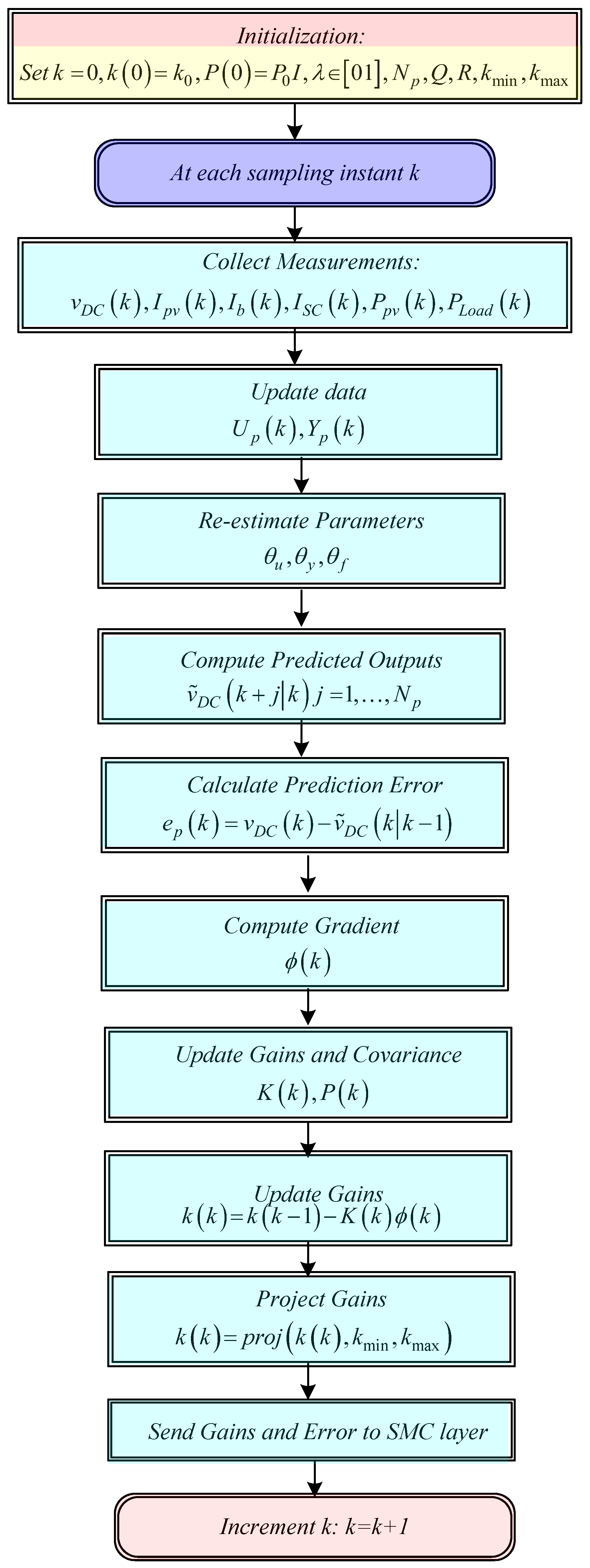
3.2. Proposed Algorithm

The proposed algorithm implements a recursive, online procedure for optimizing control gains within a data driven predictive strategy. The process begins with an initialization phase, during which the initial control gains, covariance matrix, forgetting factor, prediction horizon, weighting matrices, and admissible gain limits are established. Following this, the algorithm operates iteratively at each sampling instant.

At every iteration, current system measurements are collected and incorporated into updated data windows.

These data sets can be used, if necessary, to refine the predictor parameters through a RLS scheme. Using the updated predictor, future system outputs are estimated over the specified prediction horizon, allowing the computation of the instantaneous prediction error.

This prediction error serves as a basis for calculating the gradient of a defined performance criterion, which drives the adaptive adjustment of control gains via an update law that involves both the gain matrix and the covariance matrix. To ensure stability and boundedness, the updated gains are projected onto predefined feasible intervals. The optimized gains, along with the corresponding prediction error, are then provided to the SMC layer.

This procedure repeats at every sampling instant, enabling the controller to continuously adapt to changing system dynamics and operating conditions. A graphical representation of this entire process is presented in the flowchart of Figure 2, which clearly illustrates each step of the online gain optimization method.

3.3. Implementation Details of the Data Driven Predictor and Gain Optimization

This subsection provides the detailed implementation parameters required for full reproducibility of the data-driven predictor and the online gain optimization algorithm described above. The prediction horizon is set to N_p = 3 steps, with a sampling interval Δt = 0.1 s. This short horizon is chosen to capture the dominant dynamics of the DC microgrid while maintaining computational efficiency. The data window length is L = 20 samples, corresponding to 2 s of historical data, which provides sufficient information for the RLS estimation while remaining responsive to time-varying system behavior. The forgetting factor is set to λ = 0.99, which offers a trade-off between tracking capability (fast adaptation to changes) and noise rejection (smoothing of parameter estimates). This value is typical for RLS applications in power systems and was found to work well in our simulations. The matrix dimensions are specified as follows: U_p ∈ R^20×3: past control input matrix (20 samples × 3 duty cycles) Y_p ∈ R^20×1: past output matrix (20 samples × 1 bus voltage), H_u ∈ R^1×60: input-to-output predictor matrix, H_y ∈ R^1×20: output-to-output predictor matrix and H_f ∈R^1×3: future input predictor matrix.

The RLS covariance matrix is initialized as P(0) = 10³ I, where I is the identity matrix of appropriate dimension. This initialization ensures rapid initial convergence of the parameter estimates. To ensure persistency of excitation (PE) and prevent estimator divergence, we monitor the condition number of the covariance matrix P(k). The condition number is defined as κ(P) = λ_max (P)/λ_min (P), where λ_max and λ_min are the maximum and minimum eigenvalues of P, respectively. If the condition number exceeds a threshold of 10⁴, we partially reinitialize the covariance matrix as P(k) = 10³ I to prevent numerical instability and divergence of the estimates. This PE check is performed at each sampling instant before the gain update. The gain vector k(k) = [k_pv (k), k_b (k), k_SC (k)]^T is updated every N_opt = 2 samples (i.e., every 0.2 s) to reduce computational burden, while the SMC runs at the converter switching frequency. The gain bounds are set to k_i,min = 25 and k_i,max = 70 for all subsystems, based on physical constraints (maximum allowable switching frequency, actuator saturation limits). The performance index weights are chosen as Q = 10 (penalizing voltage deviations) and R = 0.1 (penalizing gain variations), providing a balance between fast voltage regulation and smooth gain adaptation. These weights were tuned empirically through preliminary simulations.

A sensitivity analysis was conducted to assess the impact of the forgetting factor λ on the predictor performance. Values of λ in the range [0.95, 0.995] were tested. The value λ = 0.99 was found to provide the best trade-off, yielding a prediction RMSE of 0.42 V compared to 0.51 V for λ = 0.95 and 0.48 V for λ = 0.995.

Algorithm summarizes the complete online gain optimization procedure.

Initialize:

• Initial gains: k(0) = [40, 40, 40]^T
• Covariance matrix: P(0) = 10³ I
• Forgetting factor: λ = 0.99
• Prediction horizon: N_p = 3
• Data window length: L = 20
• Gain bounds: k_min = 25, k_max = 70
• Performance index weights: Q = 10, R = 0.1

At each sampling instant k (every Δt = 0.1 s):

• Collect measurements: $y\left(k\right)= v_{DC}\left(k\right), u\left(k\right) = {\left[d_{pv}\left(k\right) d_B\left(k\right) d_{SC}\left(k\right)\right]}^T$
• Update data windows: $U_p\left(k\right) \leftarrow {\left[u\left(k-1\right) u\left(k-2\right) \cdots u\left(k-L\right)\right]}^T$ $Y_p\left(k\right) \leftarrow {\left[y\left(k-1\right) y\left(k-2\right) \cdots y\left(k-L\right)\right]}^T$
• Update predictor parameters using RLS with forgetting factor λ:

  ○

  Compute prediction error: $e_p\left(k\right)=y\left(k\right)-\widehat{y}\left(k\left|k-1\right.\right)$

  ○

  Update parameter vector θ(k) using RLS update equations

• Check persistency of excitation:

  ○

  Compute condition number κ(P(k))

  ○

  If κ(P(k)) > 10⁴, reinitialize P(k) = 10³ I

• If k mod N_opt = 0 (gain update instant):

  ○

  Compute predictions: $v_{DC}\left(k+j\left|k\right.\right)$ for $j=1,\dots ,N_p$

  ○

  Compute gradient: $\varphi \left(k\right)={\displaystyle \frac{\mathsf{\partial }{J}_p\left(k\right)}{\mathsf{\partial }k\left(k\right)}}$ (finite differences or analytical)

  ○

  Update RLS gain: $K\left(k\right)={\displaystyle \frac{P\left(k-1\right)\varphi \left(k\right)}{\lambda +{\varphi }^T\left(k\right)P\left(k-1\right)\varphi \left(k\right)}}$

  ○

  Update covariance: $P\left(k\right)={\displaystyle \frac{1}{\lambda }}\left(P\left(k-1\right)-K\left(k\right){\varphi }^T\left(k\right)P\left(k-1\right)\right)$

  ○

  Update gains: k(k) = k(k − 1) − K(k)ϕ(k)

  ○

  Project gains: k_i (k) = min(max(k_i (k), k_i,min), k_i,max) for i ∈ {pv, b, SC}

• Output: Optimized gains k(k) and prediction error ep (k) to AFSMC layer

The above parameters and procedures ensure that the data driven predictor and gain optimization algorithm can be reproduced with minimal ambiguity.

4. Adaptive Fuzzy Sliding Mode Control

This section develops the low level control layer of the proposed hybrid strategy. For each subsystem (PV, battery, SC), a sliding mode controller is designed to track a current reference provided by the EMS. To compensate for unknown nonlinearities, external disturbances, and modeling errors, fuzzy logic systems are embedded into the SMC laws. Moreover, the control gains are those optimized online by the data driven predictor (Section 3), and a prediction error feedforward term is added to enhance robustness.

4.1. Fuzzy Logic System Approximator

A fuzzy logic system with center average defuzzifier, product inference, singleton fuzzifier, and Gaussian membership functions can approximate any continuous function on a compact set to arbitrary accuracy.

The FLS output is expressed as:

$$f\left(z\right) = {\theta }^T\xi \left(z\right)$$

(10)

where $\theta = {\left[\begin{array}{ccc}{\theta }_1,& \dots ,& {\theta }_N\end{array}\right]}^T$ is the vector of adjustable consequent parameters, and $\xi \left(z\right) = {\left[{\xi }_1\left(z\right), \dots , {\xi }_N\left(z\right)\right]}^T$ is the vector of fuzzy basis functions defined by: ${\xi }_l\left(z\right)= {\displaystyle \frac{{\displaystyle {\prod }_{i=1}^n{\mu }_{F_i^l}\left(z_i\right)}}{{\displaystyle {\sum }_{j=1}^N{\displaystyle {\prod }_{i=1}^n{\mu }_{F_i^l}\left(z_i\right)}}}} , l=1, \dots , N$ with ${\mu }_{F_i^l}\left(z_i\right)= \exp \left(-{\displaystyle \frac{{\left(z_i -c_i^l\right)}^2}{{\left(b_i^l\right)}^2}}\right)$. For each subsystem i, the fuzzy logic system uses n = 5 Gaussian membership functions per input variable (negative large, negative small, zero, positive small, positive large), with centers $c_i^l$ uniformly distributed over the operating range. The number of fuzzy rules is $N=n^n$, where n_z is the dimension of z_i. For the battery subsystem, $z_b = {\left[S_b {\dot{S}}_b\right]}^T$, giving N = 25 rules.

The universal approximation property guarantees that for any continuous function h(z) on a compact set and any ϵ > 0, there exists an FLS such that $\mathit{sup}\left|h\left(z\right) - {\theta }^{\ast T}\xi \left(z\right)\right| \le \epsilon$ where ${\theta }^{\ast }$ is an optimal parameter vector.

4.2. Predictive Fuzzy Sliding Mode Control Laws

For each converter, we define a current tracking error and a sliding surface. Let the reference current for subsystem i be $I_i^{ref}$ (provided by the EMS or MPPT). The tracking error is: $z_i = I_i -I_i^{ref}, i\in \left\{pv, b, SC\right\}$.

The sliding surface is chosen as $S_i =z_i$. The control objective is to force S_i → 0 in finite time, which implies perfect current tracking.

The dynamics of S_i are obtained from the converter model (1)–(3). For example, for the PV boost converter:

$${\dot{S}}_{pv} = {\dot{I}}_{pv} - {\dot{I}}_{pv}^{ref} ={\displaystyle \frac{1}{L_{pv}}} \left(v_{pv}-\left(1-d_{pv}\right)v_{DC}\right) - {\dot{I}}_{pv}^{ref}$$

The same structure holds for the battery and SC, with their respective voltages and inductances.

In practice, the converter models contain unknown functions due to parameter uncertainties, unmodeled nonlinearities, and external disturbances.

For the PV subsystem, we lump all unknown terms into a continuous function $h_{pv}\left(z_{pv}\right)$, where $z_{pv} ={\left[x_1 \theta t\right]}^T$ may include states, parameters, and time. According to the universal approximation theorem, there exists an FLS such that:

$$h_{pv}\left(z_{pv}\right)= {\theta }_{pv}^{\ast T}{\xi }_{pv}\left(z_{pv}\right)+ {\delta }_{pv}\left(z_{pv}\right), \left|{\delta }_{pv}\right| \le {\epsilon }_{pv}$$

where ${\delta }_{pv}$ is the approximation error. Similarly, for the battery and SC, we define $h_b\left(z_b\right)$ and $h_{SC}\left(z_{SC}\right)$.

Because the optimal parameters θ^∗ are unknown, we use online estimates ${\widehat{\theta }}_i$ and design adaptive laws. The fuzzy compensator output is ${\widehat{\theta }}_i^T{\xi }_i$.

The proposed control law for each converter consists of three parts: an equivalent control term (based on the nominal model), a switching term with the optimized gain, a fuzzy adaptive compensation term, and a prediction error feedforward term. For the PV converter:

$$d_{pv} =1- {\displaystyle \frac{1}{v_{DC}}} \left(v_{pv}-L_{pv}\left({\dot{I}}_{pv}^{ref}-k_{pv}\left(k\right)sat\left({\displaystyle \frac{S_{pv}}{{\varphi }_{pv}}}\right) -{\displaystyle \frac{1}{2}}{S}_{pv}{\widehat{\theta }}_{pv}^T{\xi }_{pv} -k_{p,pv}{\widehat{e}}_p\left(k\right)\right)\right)$$

(11)

where $k_{pv}\left(k\right) > 0$ is the time varying gain optimized by Algorithm (Figure 2), $sat\left({\displaystyle \frac{S_{pv}}{{\varphi }_{pv}}}\right)$ is the saturation function replacing the sign to reduce chattering, with ϕ > 0 the boundary layer thickness, ${\widehat{\theta }}_{pv}$ is the estimate of the fuzzy parameters, $k_{p,pv} > 0$ is a predictive compensation gain, ${\widehat{e}}_p\left(k\right)$ is the one step ahead prediction error of the DC bus voltage (from Section 3). Analogous control laws are derived for the battery and SC:

$$d_b = 1-{\displaystyle \frac{1}{v_{DC}}} \left(v_b-L_b\left({\dot{I}}_b^{ref}-k_b\left(k\right)sat\left({\displaystyle \frac{S_b}{{\varphi }_b}}\right) -{\displaystyle \frac{1}{2}}{S}_b{\widehat{\theta }}_b^T{\xi }_b -k_{p,b}{\widehat{e}}_p\left(k\right)\right)\right)$$

(12)

$$d_{SC} = 1-{\displaystyle \frac{1}{v_{DC}}} \left(v_{SC}-L_{SC}\left({\dot{I}}_{SC}^{ref}-k_{SC}\left(k\right)sat\left({\displaystyle \frac{S_{SC}}{{\varphi }_{SC}}}\right) -{\displaystyle \frac{1}{2}}{S}_{SC}{\widehat{\theta }}_{SC}^T{\xi }_{SC} -k_{p,SC}{\widehat{e}}_p\left(k\right)\right)\right)$$

(13)

The predictive term $-k_{p,i}{\widehat{e}}_p\left(k\right)$ anticipates future voltage deviations and proactively adjusts the duty cycle, thereby improving transient response.

To update the fuzzy parameter estimates, we use a gradient descent approach with a σ-modification term to ensure boundedness. The adaptive law for ${\widehat{\theta }}_{pv}$ is:

$${\dot{\widehat{\theta }}}_{pv} = {\mathsf{\Gamma }}_{pv} \left({\displaystyle \frac{1}{2}}{S}_{pv}^2{v}_{SC}{\xi }_{pv}\left(z_{pv}\right)-{\sigma }_{pv}{\widehat{\theta }}_{pv} \right)$$

(14)

where ${\mathsf{\Gamma }}_{pv} = {\mathsf{\Gamma }}_{pv}^T > 0$ is a positive definite adaptation gain matrix, and ${\sigma }_{pv} > 0$ is a small constant (σ-modification). The same structure applies to ${\widehat{\theta }}_b$ and ${\widehat{\theta }}_{SC}$. The term ${\displaystyle \frac{1}{2}}{S}_i^2{\xi }_i$ comes from the Lyapunov design.

The integration of the sliding mode laws (11)–(13) with the adaptive fuzzy compensator (14) yields several synergistic benefits. The sliding mode component guarantees finite time convergence of the current tracking error despite matched uncertainties, providing inherent robustness. Meanwhile, the fuzzy compensator learns unknown nonlinear dynamics online, which reduces the required switching gain magnitude and effectively attenuates chattering. A predictive feedforward term, derived from the data driven model, anticipates future voltage deviations and pre-emptively corrects them. Finally, the time varying gains k_i (k) are optimized online, ensuring that the controller maintains peak performance even as operating conditions change.

4.3. Reference Current Generation

The reference currents ($I_{pv}^{ref}, I_b^{ref}, I_{SC}^{ref}$) are determined as follows:

A conventional perturb-and-observe maximum power point tracking algorithm provides $I_{pv}^{ref}$ to maximise the photovoltaic power output.

The high level DQL agent described in Section 5 supplies the battery and SC references $I_b^{ref}$ and $I_{SC}^{ref}$.

The agent selects appropriate charging, discharging and load shedding commands while ensuring that the combined power from the battery and SC together with the PV source and the load satisfies the bus voltage dynamics given in Equation (4).

All current references are limited to respect physical constraints such as maximum allowable battery current and SC voltage range.

4.4. Summary of the AFSMC Layer

At each sampling instant, the AFSMC layer performs the following steps:

Step 1: Receive the optimized gains $k_i\left(k\right)$ from Algorithm (Figure 2) and the prediction error ${\widehat{e}}_p\left(k\right)$ from the data driven predictor.

Step 2: Measure the actual currents I_i and compute the tracking errors $S_i =I_i- I_i^{ref}$.

Step 3: Update the fuzzy parameter estimates ${\widehat{\theta }}_i$ using (14).

Step 4: Compute the duty cycles d_i using (11)–(13) with the saturation function.

Step 5: Apply the duty cycles to the corresponding converters.

5. Augmented DQL Agent for High Level Energy Management

This section describes the learning based decision layer that coordinates the charging/discharging of the battery and SC, as well as load shedding actions. Unlike conventional DQL implementations that rely solely on instantaneous measurements [18], the proposed agent receives an augmented state vector enriched with predictive information from the data driven model. This augmentation enables anticipative policies that proactively counteract future disturbances.

In a DC microgrid subject to rapidly varying solar irradiance and load demand, decisions based only on current measurements are inherently reactive. By the time a voltage deviation is detected, the system may already be experiencing significant transients. The data driven predictor provides short term forecasts of the DC bus voltage and PV power, as well as a prediction error. Incorporating these forecasts into the agent’s state allows it to learn actions that prevent or mitigate future voltage drops or over voltages, thereby improving stability and reducing battery stress.

5.1. Extended State Representation

At each decision step, the agent perceives an augmented state vector s(t) ∈ S defined as:

$$S\left(t\right)= {\left[v_{DC}\left(t\right) P_{pv}\left(t\right) P_{load}\left(t\right) SO{C}_{bat}\left(t\right) SO{C}_{SC}\left(t\right) {\widehat{e}}_p\left(t\right) {\widehat{v}}_{DC}\left(t+\left.1\right| t\right) {\widehat{P}}_{pv}\left(t+\left.1\right| t\right)\right]}^T$$

(15)

where $v_{DC}\left(t\right)$ is the current DC bus voltage, $P_{pv}\left(t\right)$ is the current PV power, $P_{load}\left(t\right)$ is the current load demand, $SO{C}_{bat}\left(t\right) \in \left[0 1\right]$ is the battery state of charge, $SO{C}_{SC}\left(t\right) \in \left[0 1\right]$ is the SC state of charge, ${\widehat{e}}_p\left(t\right)= v_{DC}\left(t\right)-{\widehat{v}}_{DC}\left( \left.t\right| t-1\right)$ is the one step prediction error of the bus voltage (computed by the data driven predictor), ${\widehat{v}}_{DC}\left(t+\left.1\right|t\right)$ is the one step ahead prediction of the bus voltage, ${\widehat{P}}_{pv}\left(t+\left.1\right|t\right)$ is the one step ahead prediction of the PV power.

All components are normalized to the interval [0, 1] using min-max scaling to facilitate neural network training. The inclusion of ${\widehat{e}}_p\left(t\right)$ provides feedback on the predictor’s accuracy, while ${\widehat{v}}_{DC}\left(t+\left.1\right|t\right)$ and ${\widehat{P}}_{pv}\left(t+\left.1\right|t\right)$ give direct foresight of near future conditions.

The agent selects a discrete action at each decision step. The action space is designed to reflect the main energy management decisions:

$$a\left(t\right) =\left(a_{bat}, a_{SC}, a_{shed}\right)$$

(16)

where:

a_bat ∈ {charge, idle, discharge}—battery mode. The corresponding current reference $I_b^{ref}$ is then set to a predefined value (e.g., 0.2C rate) or zero, scaled by the agent’s confidence (further refined by a lower level PI or SMC).

a_SC ∈ {charge, idle, discharge} SC mode. The current reference $I_{SC}^{ref}$ is similarly determined.

a_shed ∈ {no shed, partial shed, full shed} load shedding level. Partial shed reduces the load by a fixed percentage (e.g., 30%), while full shed disconnects non critical loads.

The action space consists of 3 modes for the battery $\left(a_{bat} \in \left\{1, 2\right\}\right), 3$ modes for the SC $\left(a_{sc} \in \left\{0, 1, 2\right\}\right)$, and 3 load shedding levels $\left(a_{shed} \in \left\{0, 1, 2\right\}\right)$. The total number of discrete actions is 3 × 3 × 3 = 27. The agent can output a single integer action that encodes the combination, or use a multi-head architecture. In this work, we adopt a flat action space with 27 actions.

5.2. Reward Function Design

The reward function guides the agent toward desirable behaviors: maintaining voltage stability, preserving battery health, minimizing load shedding, and using the SC for transient peaks. The instantaneous reward r(t) is defined as:

$$r\left(t\right)= r_{volt}\left(t\right) + r_{soc}\left(t\right) + r_{shed}\left(t\right) + r_{wear}\left(t\right) + r_{pred}\left(t\right)$$

(17)

Each component is detailed below. The Voltage Regulation Reward

$$r_{volt}\left(t\right) = -{\alpha }_v{\left(v_{DC}\left(t\right) - v_{DC}^{ref}\right)}^2$$

(18)

where α_v > 0 is a weight. This term penalizes deviations from the nominal bus voltage.

The Battery SoC Preservation Reward: To avoid deep discharges and overcharging, a quadratic penalty is applied when SoC leaves a safe band $\left[so{c}_{bat}^{\mathit{min}} so{c}_{bat}^{\mathit{max}}\right]$:

$$r_{soc}\left(t\right) = -{\alpha }_{soc}\left(\mathit{max}{\left(0, so{c}_{bat}^{\mathit{min}}- so{c}_{bat}\left(t\right)\right)}^2+ \mathit{max}{\left(0, so{c}_{bat}- so{c}_{bat}^{\mathit{max}}\right)}^2\right)$$

(19)

The Load Shedding Penalty: Load shedding is allowed but penalized to encourage energy balancing without disconnection:

$$r_{shed}\left(t\right) = -{\alpha }_{shed} · l_{\left\{a_{shed\ne no shed}\right\}}$$

(20)

where l is the indicator function. Partial shedding incurs a smaller penalty than full shedding (by scaling α_shed accordingly).

The Battery Wear Reduction: High frequency charge/discharge cycles accelerate battery aging. To discourage unnecessary cycling, we penalize the absolute change in battery current reference:

$$r_{wear}\left(t\right) = -{\alpha }_{wear}\left|I_b^{ref}\left(t\right) - I_b^{ref}\left(t -1\right)\right|$$

(21)

The Predictive Term: A novel component that uses the prediction error and future voltage forecast to reward anticipative actions:

$$r_{pred}\left(t\right) = -{\alpha }_{pred}{\left({\widehat{e}}_p\left(t\right)\right)}^2 -{\alpha }_{fu} {\left(v_{DC}\left(t+\left.1\right|t\right) - v_{DC}^{ref}\right)}^2$$

(22)

This term encourages the agent to keep both the current prediction error and the predicted future voltage small, thereby learning to act before a voltage deviation actually occurs. All weights α_v, α_soc, α_shed, α_wear, α_pred, α_fut are positive constants chosen empirically to balance the objectives.

5.3. Deep Q-Learning Architecture and Training Algorithm

The agent uses a Deep Q-Network (DQN) to approximate the action value function $Q\left(s, a , \theta \right)$, where θ are the network weights. The network architecture consists of:

Input layer: 8 neurons (one per augmented state component).

Two hidden layers, each with 128 neurons and ReLU activation.

Output layer: 27 neurons (one per action) with linear activation.

The DQN is trained using experience replay and a target network to stabilize learning. At each decision step, the agent selects an action according to an ϵ-greedy policy: with probability ϵ it explores uniformly, otherwise it chooses the action with the highest Q-value.

We adopt the standard DQN architecture [19], where the action-value function is approximated by a neural network. Throughout the paper, we refer to this approach as DQL for consistency with the reinforcement learning literature.

The DQL agent is trained offline in a high fidelity MATLAB (2023 b)/Simulink simulator that implements the full DCMG model (5), the AFSMC layer, the data driven predictor, and the gain optimization algorithm. Training episodes are designed to cover a wide range of operating conditions:

PV power profiles: sinusoidal variations (diurnal cycles), step changes (cloud passages), and random fluctuations (stochastic weather).

Load profiles: slow ramps, abrupt steps, and pseudo random sequences.

Initial conditions: random SoC_bat and SoC_SC within [0.2, 0.9] and [0.3, 0.8] respectively.

The main hyperparameters used in the DQL model are as follows: the learning rate is set to 0.001, and the discount factor (γ) is fixed at 0.95. The exploration strategy begins with an initial exploration rate (ϵ₀) of 1.0, which gradually decays to a final value (ϵ_min) of 0.01 using a decay rate of 0.995 per episode. The experience replay buffer has a capacity of 50,000 transitions, from which mini-batches of size 64 are sampled during training. Additionally, the target network is updated every 100 episodes to stabilize learning. The model is trained over a total of 3000 episodes.

The training proceeds as follows:

Step 1: Initialize the Q-network with random weights, and copy them to the target network.

Step 2: For each episode:

○

Reset the simulation environment to a random initial state.

○

For each decision step t:

▪

Observe augmented state s(t).

▪

Select action a(t) using ϵ-greedy.

▪

Apply the action to the AFSMC layer (which translates it into current references $I_b^{ref}, I_{SC}^{ref}$ and load shedding command).

▪

Run the microgrid simulation for the decision interval (0.1 s).

▪

Compute reward r(t) and observe next state s(t + 1).

▪

Store transition (s(t), a(t), r(t), s(t + 1)) in replay buffer.

▪

Sample a random mini-batch from the buffer and update the Q-network by minimizing the temporal difference loss:

$$L = E \left[{\left(r+ \gamma \underset{a^{\prime }}{\mathit{max}}{Q}_{\mathit{target}}\left(s^{\prime }, a^{\prime }\right) - Q\left(s, a\right)\right)}^2\right]$$

(23)

○

End episode.

○

Decay ϵ.

○

Every 100 episodes, update target network weights.

After convergence (typically around 2500–3000 episodes), the agent’s policy is frozen and used for validation.

5.4. Integration with Lower Control Layers

The DQL agent outputs a discrete action a(t) = (a_bat, a_SC, a_shed) at each decision step. The mapping from DQL actions to reference currents is defined as follows (

Table 1. DQL action mapping to reference currents and load shedding levels.

Action abat	Battery Mode	${\mathit{I}}_{\mathit{b}}^{\mathit{r}\mathit{e}\mathit{f}}$
0	Charge (C/2 rate)	+5 A
1	Idle	0 A
2	Discharge (C/2 rate)	−5 A
Action aSC	SC Mode	$I_{SC}^{ref}$
0	Charge (5 A)	+5 A
1	Idle	0 A
2	Discharge (5 A)	−5 A
Action ashed	Load Shedding Level	Load Reduction
0	No shed	0%
1	Partial shed	30%
2	Full shed	100% (non critical loads)

):

The reference currents are further adjusted based on the current SOC to prevent overcharging or deep discharge:

$$I_b^{ref}= M_b\left(a_{bat}, SO{C}_{bat}\right) = \left\{\begin{array}{l}\mathit{min}\left(I_b^{ref,action}, I_{b,\mathit{max}}{\displaystyle \frac{SO{C}_{bat}^{\mathit{max}}-SO{C}_{bat}}{SO{C}_{bat}^{\mathit{max}}-SO{C}_{bat}^{\mathit{min}}}}\right) if a_{bat}=\mathit{charge}\\ \mathit{max}\left(I_b^{ref,action}, -I_{b,\mathit{max}}{\displaystyle \frac{SO{C}_{bat}-SO{C}_{bat}^{\mathit{min}}}{SO{C}_{bat}^{\mathit{max}}-SO{C}_{bat}^{\mathit{min}}}}\right) if a_{bat}=\mathit{discharge}\end{array}\right.$$

where $I_{b,\mathit{max}}= 10A$ is the maximum battery current. The SC current reference is similarly adjusted with $I_{SC,\mathit{max}}= 15A$:

$$I_{SC}^{ref}= M_{SC}\left(a_{SC}, SO{C}_{SC}\right) = \left\{\begin{array}{l}\mathit{min}\left(I_{SC}^{ref,action}, I_{b,\mathit{max}}{\displaystyle \frac{SO{C}_{SC}^{\mathit{max}}-SO{C}_{SC}}{SO{C}_{SC}^{\mathit{max}}-SO{C}_{SC}^{\mathit{min}}}}\right) if a_{SC}=\mathit{charge}\\ \mathit{max}\left(I_{SC}^{ref,action}, -I_{SC,\mathit{max}}{\displaystyle \frac{SO{C}_{SC}-SO{C}_{SC}^{\mathit{min}}}{SO{C}_{SC}^{\mathit{max}}-SO{C}_{SC}^{\mathit{min}}}}\right) if a_{SC}=\mathit{discharge}\end{array}\right.$$

The AFSMC layer then tracks these current references using the sliding mode control laws (11)–(13), which guarantee finite-time convergence of the actual currents I_i to their references $I_i^{ref}$. The load shedding command is implemented by reducing the load power according to the selected level:

$$P_{load}^{new}= \left\{\begin{array}{l}{P}_{load}^{original} if a_{shed} = 0 \left(no shed\right)\\ 0.7 \times P_{load}^{original} if a_{shed} = 1 \left(partial shed\right) \\ 0 if a_{shed} = 2 \left(full shed\right) \end{array}\right.$$

where non critical loads are disconnected first in the case of partial shedding.

At each decision step, the agent outputs:

• Battery mode: the corresponding reference current $I_b^{ref}$ is set to a predefined value.
• SC mode: similarly, $I_{SC}^{ref}$ is set to a fixed magnitude.
• Load shedding command: the load is reduced by the specified amount.

These references are then tracked by the AFSMC layer. Importantly, the SC is primarily used for fast transients, while the battery supplies sustained power. The agent learns to coordinate both to keep the bus voltage stable and the SoC levels balanced.

The proposed high level layer is a DQL agent whose state is augmented with one step predictions and the prediction error of the DC bus voltage and PV power. It learns to select discrete actions (battery mode, SC mode, load shedding level) that optimize a multiobjective reward function. The agent is trained offline in a detailed simulation environment and then deployed in conjunction with the AFSMC and the online gain optimizer. This hierarchical, predictive, learning based architecture constitutes the main novelty of the paper.

6. Stability Analysis

The stability analysis focuses on the low level AFSMC layer, assuming that the reference currents generated by the DQL agent are bounded and piecewise continuous—a condition physically guaranteed by converter limits and the agent’s bounded action space. The data driven predictor provides a bounded prediction error ${\widehat{e}}_p\left(k\right)$ (Lemma 1), and the optimized gains k_i (k) are kept within a compact interval by projection. The boundedness of the inner-loop tracking errors then implies boundedness of the DC bus voltage dynamics (4), ensuring overall stability in a cascade sense. The control objective is to force the inductor currents $I_{pv}^{ref}, I_b^{ref}, I_{SC}^{ref}$ to track their respective references while maintaining v_DC close to its nominal value $v_{DC}^{ref}$. The following assumptions are made:

Assumption 5.

The reference signals $I_{pv}^{ref}, I_b^{ref}, I_{SC}^{ref}$ and their first derivatives are bounded and have bounded second derivatives.

Assumption 6.

The unknown functions $h_i\left(z_i\right)$ (lumping parameter uncertainties, nonlinearities, and disturbances) are continuous on a compact set and can be approximated by fuzzy logic systems as in (10) with approximation errors $\left|{\delta }_i\right| \le {\epsilon }_i$ where ϵ_i are known constants.

Assumption 7.

The prediction error  $e_p\left(k\right) = v_{DC}\left(k\right) - {\widehat{v}}_{DC}\left(\left.k\right| k-1\right)$ satisfies $\left|e_p\left(k\right)\right| \le {\overline{e}}_p$ for all k with ${\overline{e}}_p$ a positive constant (Lemma 1). The continuous time analog is $\left|e_p\left(t\right)\right| \le {\overline{e}}_p$ almost everywhere.

Assumption 8.

The optimized gains k_i (t) are bounded: $0< k_{i,\mathit{min}} \le k_i\left(t\right)\le k_{i,\mathit{max}}$ due to the projection operation in Algorithm (Figure 2).

6.1. Tracking Error Dynamics for a Generic Subsystem

We analyze one subsystem (e.g., the battery) and then combine them via a composite Lyapunov function. The extension to PV and SC is identical. For the battery, define the tracking error $z_b = I_b -I_b^{ref}$. The sliding surface is $S_b =z_b$. From (2), the error dynamics are:

$${\dot{S}}_b = {\dot{I}}_b - {\dot{I}}_b^{ref} ={\displaystyle \frac{1}{L_b}} \left(v_b-\left(1-d_b\right)v_{DC}\right) - {\dot{I}}_b^{ref}$$

(24)

The unknown dynamics are lumped into a continuous function $h_b\left(z_b\right)$ such that:

$${\dot{S}}_b = {\displaystyle \frac{1}{L_b}} \left(v_b-\left(1-d_b\right)v_{DC}\right) - {\dot{I}}_b^{ref}+h_b\left(z_b\right)$$

(25)

But it is more convenient to write the actual plant as:

$${\dot{I}}_b = f_b\left(I_b, v_b, v_{DC}, d_b\right) + {\mathsf{\Delta }}_b\left(t\right)$$

(26)

where Δ_b (t) represents unknown disturbances. After substituting the control law (12) and using the fact that the fuzzy system approximates the unknown part, the closed loop error dynamics become:

$${\dot{S}}_b = -k_b\left(t\right) sat\left({\displaystyle \frac{S_b}{{\varphi }_b}}\right) - {\displaystyle \frac{1}{2}}{S}_b{\widehat{\theta }}_b^T{\xi }_b - k_{p,b}{\widehat{e}}_p\left(t\right) + {\tilde{h}}_b+ {\delta }_b$$

(27)

where ${\tilde{h}}_b = h_b -{\widehat{\theta }}_b^T{\xi }_b$ is the fuzzy approximation error, and ${\delta }_b$ is the bounded residual due to the predictor error and unmodeled terms. With the optimal parameter ${\theta }_b^{\ast }$ defined as the best approximator, we have $h_b ={\theta }_b^{\ast T}{\xi }_b + {\epsilon }_b$, with $\left|{\epsilon }_b \right| \le {\epsilon }_{b 0}$. Define the parameter estimation error ${\tilde{\theta }}_b = {\theta }_b^{\ast } -{\widehat{\theta }}_b$. Then ${\tilde{h}}_b ={\tilde{\theta }}_b^T{\xi }_b + {\epsilon }_b$.

Thus:

$${\dot{S}}_b = -k_b\left(t\right) sat\left({\displaystyle \frac{S_b}{{\varphi }_b}}\right) - {\displaystyle \frac{1}{2}}{S}_b{\widehat{\theta }}_b^T{\xi }_b - {\tilde{\theta }}_b^T{\xi }_b + {\epsilon }_b +k_{p,b}{\widehat{e}}_p\left(t\right)$$

(28)

6.2. Composite Lyapunov Function

For the whole microgrid, define the composite Lyapunov function:

$$V = {\displaystyle \frac{1}{2}} {\displaystyle \sum _{i\in \left\{pv, b, SC\right\}}{S}_i^2}+ {\displaystyle \frac{1}{2}}{\displaystyle \sum _i{\tilde{\theta }}_i^T{\mathsf{\Gamma }}_i^{-1}{\tilde{\theta }}_i}+ {\displaystyle \frac{1}{2\beta }}{e}_p^2$$

(29)

where β > 0 is a weighting coefficient, and the term ${\displaystyle \frac{1}{2\beta }}{e}_p^2$ accounts for the prediction error dynamics. Taking the time derivative along the trajectories:

$$\dot{V} = {\displaystyle \sum _i{S}_i{\dot{S}}_i}-{\displaystyle \sum _i{\tilde{\theta }}_i^T{\mathsf{\Gamma }}_i^{-1}{\dot{\widehat{\theta }}}_i}+ {\displaystyle \frac{1}{2\beta }}{e}_p{\dot{e}}_p$$

(30)

Insert the expression for S_i and the adaptive law (14) (rewritten in continuous time):

$${\dot{\widehat{\theta }}}_i = {\mathsf{\Gamma }}_i\left({\displaystyle \frac{1}{2}}{S}_i^2{\xi }_i - {\sigma }_i{\widehat{\theta }}_i\right)$$

(31)

This continuous-time formulation is used for the Lyapunov analysis. The discrete-time implementation of the adaptive law (14) is interpreted as a sampled-data approximation of (31) with sufficiently small sampling period Δt. Under standard assumptions on the system’s dynamics (Lipschitz continuity of the vector fields) and with Δt chosen sufficiently small, the continuous-time stability guarantees imply practical stability of the sampled data implementation [25].

From the closed-loop error dynamics (32), multiplying by S_i yields the following expression:

$${\dot{S}}_i= -k_{i}sat\left({\displaystyle \frac{S_i}{{\varphi }_i}}\right) - {\displaystyle \frac{1}{2}}{S}_i{\widehat{\theta }}_i^T{\xi }_i+{\tilde{\theta }}_i^T{\xi }_i+{\epsilon }_i- k_{p,i}{\widehat{e}}_p$$

(32)

Multiplying (32) by S_i yields:

$$S_i\dot{S}- {\tilde{\theta }}_i^T{\mathsf{\Gamma }}_i^{-1}{\dot{\widehat{\theta }}}_i = -k_i{S}_{i}sat\left({\displaystyle \frac{S_i}{{\varphi }_i}}\right)-{\displaystyle \frac{1}{2}}{S}_i^2{\tilde{\theta }}_i^T{\xi }_i+S_i{\epsilon }_i- k_{p,i}{S}_i{\widehat{e}}_p+S_i{\theta }_i^{\ast T}{\xi }_i$$

(33)

Using (31) and (32), we compute:

$$S_i\dot{S}- {\tilde{\theta }}_i^T{\mathsf{\Gamma }}_i^{-1}{\dot{\widehat{\theta }}}_i = -k_i{S}_{i}sat\left({\displaystyle \frac{S_i}{{\varphi }_i}}\right)-{\displaystyle \frac{1}{2}}{S}_i^2{\tilde{\theta }}_i^T{\xi }_i+S_i{\epsilon }_i- k_{p,i}{S}_i{\widehat{e}}_p+S_i{\theta }_i^{\ast T}{\xi }_i-{\sigma }_i{\tilde{\theta }}_i^T{\xi }_i{\widehat{\theta }}_i$$

(34)

where we used the fact that ${\widehat{\theta }}_i+ {\tilde{\theta }}_i= {\theta }_i^{\ast }$. The terms $-{\displaystyle \frac{1}{2}}{S}_i^2{\tilde{\theta }}_i^T{\xi }_i$ is bounded since ${\theta }_i^{\ast }$ is constant and $‖{\xi }_i‖ \le 1$. Let $M_{\theta }=\mathit{sup}‖{\theta }_i^{\ast }‖$. Then

$$-{\displaystyle \frac{1}{2}}{S}_i^2{\theta }_i^{\ast T}{\xi }_i\le {\displaystyle \frac{1}{2}}{M}_{\theta }{S}_i^2$$

(35)

Using Young’s inequality:

$$S_i{\tilde{\theta }}_i^T{\xi }_i\le {\displaystyle \frac{1}{2}}{S}_i^2+ {\displaystyle \frac{1}{2}}‖{\tilde{\theta }}_i^2‖$$

(36)

and

$$S_i{\epsilon }_i\le {\displaystyle \frac{1}{2}}{S}_i^2+ {\displaystyle \frac{1}{2}}{\epsilon }_i^2$$

(37)

$$-k_{p,i}{S}_i{\widehat{e}}_p\le {\displaystyle \frac{k_{p,i}}{2}}{S}_i^2 + {\displaystyle \frac{k_{p,i}}{2}}{\overline{e}}_p^2$$

(38)

we obtain:

$$S_i\dot{S}- {\tilde{\theta }}_i^T{\mathsf{\Gamma }}_i^{-1}{\dot{\widehat{\theta }}}_i = -k_i{S}_{i}sat\left({\displaystyle \frac{S_i}{{\varphi }_i}}\right)-{\displaystyle \frac{1}{2}}{S}_i^2{\tilde{\theta }}_i^T{\xi }_i+S_i{\epsilon }_i- k_{p,i}{S}_i{\widehat{e}}_p-{\displaystyle \frac{1}{2}}{S}_i^2{\tilde{\theta }}_i^T{\xi }_i + {\sigma }_i{\tilde{\theta }}_i^T{\widehat{\theta }}_i$$

(39)

Simplifying:

$$S_i{\dot{S}}_i- {\tilde{\theta }}_i^T{\mathsf{\Gamma }}_i^{-1}{\dot{\widehat{\theta }}}_i\le -k_i{S}_{i}sat\left({\displaystyle \frac{S_i}{{\varphi }_i}}\right) +{\displaystyle \frac{1}{2}}\left( 2+ M_{\theta }+k_{p,i}\right)S_i^2 + {\displaystyle \frac{1}{2}}{‖{\tilde{\theta }}_i‖}^2+ {\displaystyle \frac{1}{2}}{\epsilon }_i^2+ {\displaystyle \frac{k_{p,i}}{2}}{\overline{e}}_p^2 + {\sigma }_i{\tilde{\theta }}_i^T{\widehat{\theta }}_i$$

(40)

The transition from (40) to (45) requires that k_i be chosen sufficiently large. Specifically, using the saturation property:

$$-k_i{S}_{i}sat\left({\displaystyle \frac{S_i}{{\varphi }_i}}\right) \le {\displaystyle \frac{k_i}{{\varphi }_i}}{S}_i^2 \mathrm{for} \left|S_i\right| \le {\varphi }_i$$

(41)

$$-k_i{S}_{i}sat\left({\displaystyle \frac{S_i}{{\varphi }_i}}\right) \le -k_i\left|S_i\right| \mathrm{for} \left|S_i\right| >{\varphi }_i$$

(42)

By selecting k_i such that:

$${\displaystyle \frac{k_i}{{\varphi }_i}}\ge {\displaystyle \frac{1}{2}}\left( 2+ M_{\theta }+k_{p,i}\right)+ {\displaystyle \frac{1}{2}}+{\eta }_i$$

(43)

for ∣Si∣ > ϕ_i,

$$k_i\ge {\displaystyle \frac{1}{2}}\left( 2+ M_{\theta }+k_{p,i}\right)+ {\displaystyle \frac{1}{2}}+{\eta }_i$$

(44)

where η_i > 0 is a design constant and $M_{\theta }= \mathit{sup}‖{\theta }_i^{\ast }‖$, we guarantee the negativity condition. This condition is explicitly verifiable as all terms are bounded. With this gain selection, we obtain:

$$S_i{\dot{S}}_i- {\tilde{\theta }}_i^T{\mathsf{\Gamma }}_i^{-1}{\dot{\widehat{\theta }}}_i\le - {\eta }_i{S}_i^2 - {\displaystyle \frac{1}{2}}{‖{\tilde{\theta }}_i‖}^2+{\displaystyle \frac{1}{2}}{\epsilon }_i^2+{\displaystyle \frac{ k_{p,i}}{2}}{\overline{e}}_p^2 + {\sigma }_i{\tilde{\theta }}_i^T{\widehat{\theta }}_i$$

(45)

Using the identity ${\sigma }_i{\tilde{\theta }}_i^T{\widehat{\theta }}_i= {\sigma }_i{\tilde{\theta }}_i^T\left({\theta }_i^{\ast }-{\tilde{\theta }}_i\right) \le -{\displaystyle \frac{{\sigma }_i}{2}}{‖{\tilde{\theta }}_i‖}^2+ {\displaystyle \frac{{\sigma }_i}{2}}{‖{\theta }_i^{\ast }‖}^2$, we get:

$$S_i{\dot{S}}_i- {\tilde{\theta }}_i^T{\mathsf{\Gamma }}_i^{-1}{\dot{\widehat{\theta }}}_i\le - {\eta }_i{S}_i^2 -{\displaystyle \frac{{\sigma }_i-1}{2}}{‖{\tilde{\theta }}_i‖}^2+{\displaystyle \frac{1}{2}}{\epsilon }_i^2+{\displaystyle \frac{ k_{p,i}}{2}}{\overline{e}}_p^2 + {\displaystyle \frac{{\sigma }_i}{2}}{‖{\theta }_i^{\ast }‖}^2$$

(46)

where we have chosen σ_i > 1 to ensure negativity of the ${‖{\tilde{\theta }}_i‖}^2$ term. The prediction error term satisfies:

$${\displaystyle \frac{1}{\beta }}{e}_p{\dot{e}}_p \le -{\displaystyle \frac{\gamma }{\beta }}{e}_p^2+{\displaystyle \frac{M_p}{\beta }}$$

(47)

where γ > 0 and M_p > 0 are constants.

Summing over all subsystems and adding the prediction error term:

$$\dot{V}\le -{\displaystyle \sum _i{\eta }_i{S}_i^2-{\displaystyle \sum _i\frac{\left({\sigma }_i-1\right)}{2}{‖{\tilde{\theta }}_i‖}^2-\frac{\gamma }{\beta }{e}_p^2+{\displaystyle \sum \left(\frac{1}{2}{\epsilon }_i^2+\frac{k_{p,i}}{2}{\overline{e}}_p^2+ \frac{{\sigma }_i}{2}{‖{\theta }_i^{\ast }‖}^2\right)}}}+ {\displaystyle \frac{M_p}{\beta }}$$

(48)

Define:

$$\alpha =\mathit{min}\left\{2{\eta }_i,{\displaystyle \frac{\left({\sigma }_i-1\right)}{{\lambda }_{\mathit{max}}\left({\mathsf{\Gamma }}_i^{-1}\right)}}, {\displaystyle \frac{2\gamma }{\beta }} \right\}> 0$$

(49)

and

$$M={\displaystyle \sum \left(\frac{1}{2}{\epsilon }_i^2+\frac{k_{p,i}}{2}{\overline{e}}_p^2+ \frac{{\sigma }_i}{2}{‖{\theta }_i^{\ast }‖}^2\right)}+ {\displaystyle \frac{M_p}{\beta }}$$

(50)

Then:

$$\dot{V} \le -\alpha V+M$$

(51)

Applying the comparison lemma to (51) yields:

$$\dot{V} \le e^{-\alpha t}V\left(0\right)+ {\displaystyle \frac{M^{\prime }}{\alpha }}\left(1-e^{-\alpha t}\right)$$

(52)

Therefore, V(t) is uniformly ultimately bounded with:

$$\underset{t\to \infty }{\mathit{lim}} \mathit{sup}V\left(t\right) \le {\displaystyle \frac{M}{\alpha }}$$

(53)

Since $V\left(t\right) \ge {\displaystyle \frac{1}{2}} {\displaystyle \sum _i{S}_i^2}$, the tracking errors converge to the residual set:

$$\left|S_i\right| \le \sqrt{{\displaystyle \frac{2M^{\prime }}{\alpha }}} \mathrm{for} \mathrm{all} i$$

(54)

which can be made arbitrarily small by increasing k_i (i.e., increasing η_i) and reducing approximation errors.

Which can be made arbitrarily small by increasing the control gains (within the projection bounds) and reducing the approximation errors (by using more fuzzy rules or better predictor).

The online gain optimization Algorithm (Figure 2) maintains $k_i\left(t\right)$ within $\left[k_{i,\mathit{min} } k_{i,\mathit{max} }\right]$. The analysis above only requires $k_i\left(t\right) \ge k_{i,\mathit{min}}$ sufficiently large to satisfy the inequality $k_i{S}_{i}sat\left(S_i/{\varphi }_i\right) \le -{\eta }_i{S}_i^2$. Since the projection ensures $k_i\left(t\right) \ge k_{i,\mathit{min}}$, stability is preserved as long as $k_{i,\mathit{min}}$ is chosen large enough. The optimization actually increases $k_i\left(t\right)$ when needed (e.g., during transients), which further improves convergence.

Thus, under the assumption of bounded piecewise continuous reference currents, the AFSMC inner loop guarantees uniform ultimate boundedness of the tracking errors and parameter estimation errors. Since the DQL agent’s actions are bounded by construction and the reference currents are physically limited, the cascade interconnection ensures boundedness of all signals of the overall system.

The following theorem summarizes the stability properties.

Theorem 1.

Consider the DC microgrid (5) under the AFSMC laws (11)–(13), the adaptive laws (14), and the data driven predictor providing bounded prediction error ${\widehat{e}}_p$ with $\left|{\widehat{e}}_p\right| \le {\overline{e}}_p$. Suppose Assumptions 5–8 hold and the initial conditions are bounded. Assume further that the reference currents $I_{pv}^{ref}, I_b^{ref}, I_{SC}^{ref}$ are bounded and piecewise continuous a condition physically guaranteed by the DQL agent’s action constraints (e.g., maximum converter currents, SoC limits). Then:

i. 

All signals in the low-level AFSMC inner loop, including the tracking errors S_i and the fuzzy parameter estimation errors ${\tilde{\theta }}_i$, are uniformly bounded.

ii. 

The tracking errors converge to a residual set ${\mathsf{\Omega }}_i =\left\{\left|S_i\right| \le \sqrt{2M^{\prime }/\alpha }\right\}$  where $M^{\prime }$ depends on the approximation errors and the bound on ${\widehat{e}}_p$, and α is a positive constant determined by the control gains and adaptation parameters.

iii. 

By increasing the minimum allowable gain $k_{i,\mathit{min}}$ and improving the fuzzy approximation (reducing ϵ_i), the residual set can be made arbitrarily small.

iv. 

Since the DQL agent operates at a slower timescale and its actions are bounded by physical converter limits, the reference currents remain bounded. Consequently, the boundedness of the inner-loop tracking errors implies the boundedness of the DC bus voltage dynamics (4), ensuring overall closed-loop stability in a cascade sense.

Proof of Theorem 1.

We analyze one subsystem (e.g., the battery) and then combine them via a composite Lyapunov function. The extension to PV and SC is identical. For the battery, define the tracking error $z_b = I_b-I_b^{ref}$. The sliding surface is S_b = z_b. From (2), the error dynamics are (24). The unknown dynamics are lumped into a continuous function h_b (z_b). With the optimal parameter ${\theta }_b^{\ast }$ defined as the best approximator, we have $h_b= {\theta }_b^{\ast T}{\xi }_b + {\epsilon }_b$, with $\left|{\epsilon }_b\right| \le {\epsilon }_{b0}$. Define the parameter estimation error ${\tilde{\theta }}_b={\theta }_b^{\ast }-{\widehat{\theta }}_b$. □

After substituting the control law (12) and using the fact that the fuzzy system approximates the unknown part, the closed-loop error dynamics become (42).

For the whole microgrid, define the composite Lyapunov function (29) where β > 0 is a weighting coefficient, and the term ${\displaystyle \frac{1}{2\beta }}{e}_p^2$ accounts for the prediction error dynamics.

Taking the time derivative along the trajectories (30).

The adaptive law is (32) Using (42) and (32), and computing $S_i{\dot{S}}_i-{\tilde{\theta }}_b^T{\mathsf{\Gamma }}_i^{-1}{\widehat{\dot{\theta }}}_i$, we obtain (39). Using the saturation property (51) and (52). Using Young’s inequality and the boundedness of the fuzzy basis functions (∣ξ_i∣ ≤ 1) ((37), (48) and (53)).

By selecting k_i and k_p,i sufficiently large (within the projection bounds [k_i,min, k_i,max]) such that: ($k_i \ge {\displaystyle \frac{{\varphi }_i}{2}}\left(1+k_{p,i}+ {\eta }_i\right)$: inside boundary layer) and ($k_i \ge {\displaystyle \frac{1}{2}}\left(1+k_{p,i}+ {\eta }_i\right)$: outside boundary layer) where η_i > 0 is a design constant, we can show that (54). The prediction error dynamics satisfy (56) where γ > 0 is a positive constant and M_p > 0 depends on the boundedness of the system signals and the predictor dynamics. This boundedness follows from Lemma 1 and the fact that all signals in the closed-loop system remain bounded as shown below. Then:

$$\dot{V}\le -\alpha V+M$$

(55)

Applying the comparison lemma to (61) yields:

$$V\left(t\right)\le V\left(0\right)e^{-\alpha t}+{\displaystyle \frac{M}{\alpha }}\left(1-e^{-\alpha t}\right)$$

(56)

Therefore, V(t) is uniformly ultimately bounded with:

$$\underset{t\to \infty }{\mathit{lim}}V\left(t\right)\le {\displaystyle \frac{M}{\alpha }}$$

(57)

Since $V\left(t\right)\ge {\displaystyle \frac{1}{2}}{\displaystyle {\sum }_i{S}_i^2}$, we have:

$${\displaystyle {\sum }_i{S}_i^2} \le 2V\left(t\right)\le 2V\left(0\right)e^{-\alpha t}+ {\displaystyle \frac{2M}{\alpha }}$$

(58)

Thus:

$$\underset{t\to \infty }{\mathit{lim} \mathit{sup}}{\displaystyle {\sum }_i{S}_i^2} \le {\displaystyle \frac{2M}{\alpha }}$$

(59)

Therefore, the tracking errors converge to the residual set (54).

Since the DQL agent operates at a slower timescale and its actions are bounded by converter limits (e.g., I_b ≤ I_b,max, SOC ∈ [SOC_min, SOC_max]), the reference currents $I_i^{ref}$ are bounded and piecewise continuous. The above analysis guarantees that the actual currents I_i track these references with bounded errors. From the DC bus voltage dynamics (4). Since all currents Ii, duty cycles d_i, and load current I_Load are bounded (the latter by physical limits), the right-hand side of (4) is bounded. Therefore, the bus voltage v_DC remains bounded. This establishes overall closed-loop stability in a cascade sense.

7. Simulation Results

This section presents a comprehensive simulation study to validate the proposed data driven predictive hybrid control strategy. The performance of the proposed approach is compared against two strategies: (i) a conventional fuzzy logic based energy management system coupled with a fixed gain SMC (FLC method) [15] and (ii) a standard DQL agent with only instantaneous state information combined with fixed gain SMC (DQL method) [20]. The two strategies (FLC and DQL) both employ fixed- gain sliding mode controllers, whereas our method benefits from online gain optimization and an augmented DQL state.

All simulations are carried out in MATLAB using the averaged model of the DC microgrid described in Section 2. The microgrid parameters are as follows: nominal DC bus voltage v_DCref = 48 V; PV boost converter L_pv = 3 mH, C_pv = 1000 μF; battery bidirectional converter L_b = 3 mH, C_b = 1000 μF, battery nominal voltage v_b = 36 V, capacity 100 Ah; SC converter L_SC = 2 mH, C_SC = 2000 μF, SC bank rated at 30 F; DC bus capacitance C_DC = 2200 μF; load resistive, variable from 0 to 2 kW.

For the proposed method, the adaptive fuzzy SMC gains are initialised to k_pv (0) = k_b (0) = k_SC (0) = 40 with bounds [25, 70]. The saturation boundary layer thickness is ϕ = 0.15, predictive compensation gains are k_p,pv = k_p,b = k_p,SC = 2. The data driven predictor uses a window length L = 20, prediction horizon N_p = 3 and forgetting factor λ = 0.99. The DQL agent is trained for 3000 episodes.

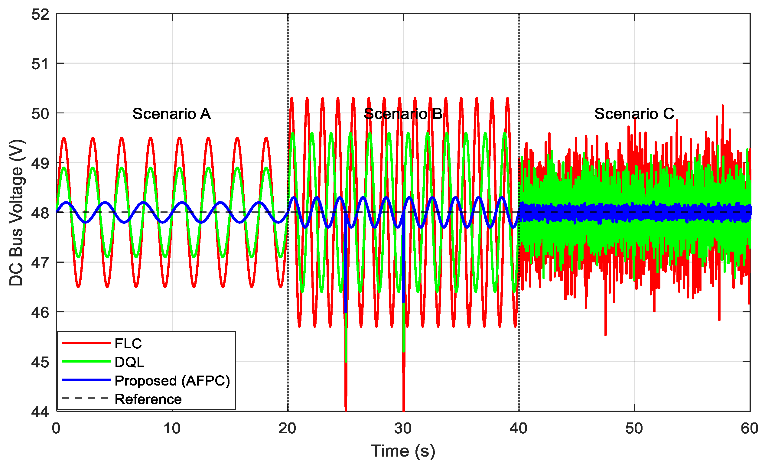
The three test scenarios are concatenated on a single time axis: Scenario A (0–20 s, sinusoidal variations), Scenario B (20–40 s, step changes) and Scenario C (40–60 s, stochastic fluctuations). An additional extreme disturbance scenario (Scenario D) is simulated separately for robustness assessment.

Scenario A: Smooth Sinusoidal Variations.

The performance under slowly varying PV power and load. The proposed method reduces the voltage RMSE from 1.24 V (FLC) and 0.91 V (standard DQL) to only 0.42 V, an improvement of 66% and 54% respectively. The maximum voltage deviation is cut by more than half, from 2.7 V to 0.9 V. Battery stress (integral of |I_b|) is reduced by 62% compared to the fuzzy, and load shedding is completely eliminated. These gains stem from the adaptive fuzzy compensation and the predictive feedforward term, which anticipate the slow oscillations and keep the bus voltage tightly regulated.

Scenario B: Step Changes (PV drop and load step).

Figure 3 shows the DC bus voltage response of the three controllers during the concatenated scenarios, with a particular focus on the step disturbances at t = 25 s (PV drop from 1000 W to 300 W) and t = 30 s (load step from 500 W to 1200 W). The proposed method exhibits the smallest voltage dip (2.1 V vs. 4.3 V for FLC and 3.0 V for standard DQL) and the fastest settling time (0.22 s vs. 0.65 s and 0.38 s).

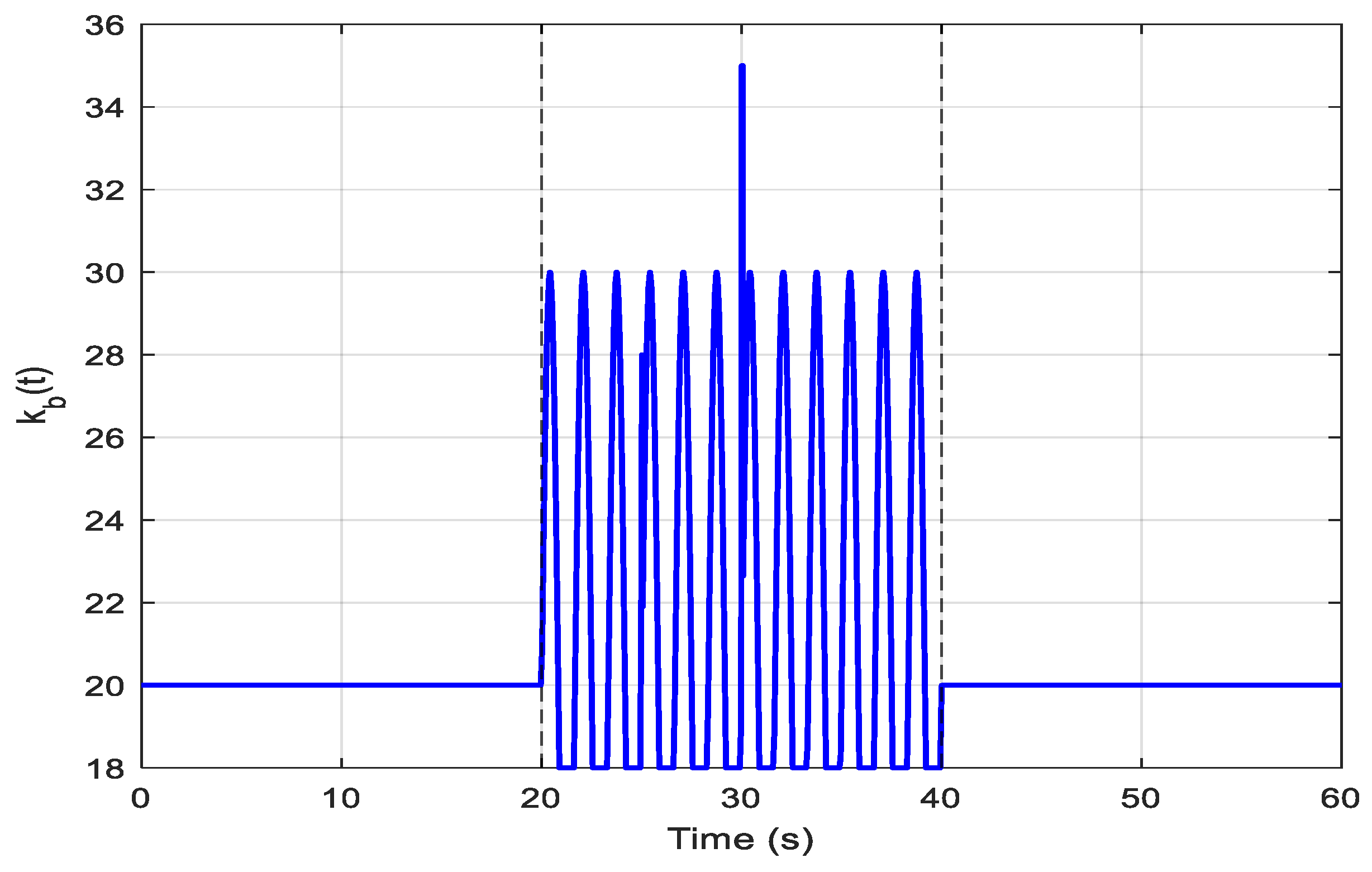
The improved performance is attributed to the online gain optimisation (Figure 4) and the prediction error feedforward. As seen in Figure 5, the battery SMC gain k_b (t) rises from 20 to 28 within 0.04 s after the PV drop and further to 35 during the load step, providing extra robustness exactly when needed.

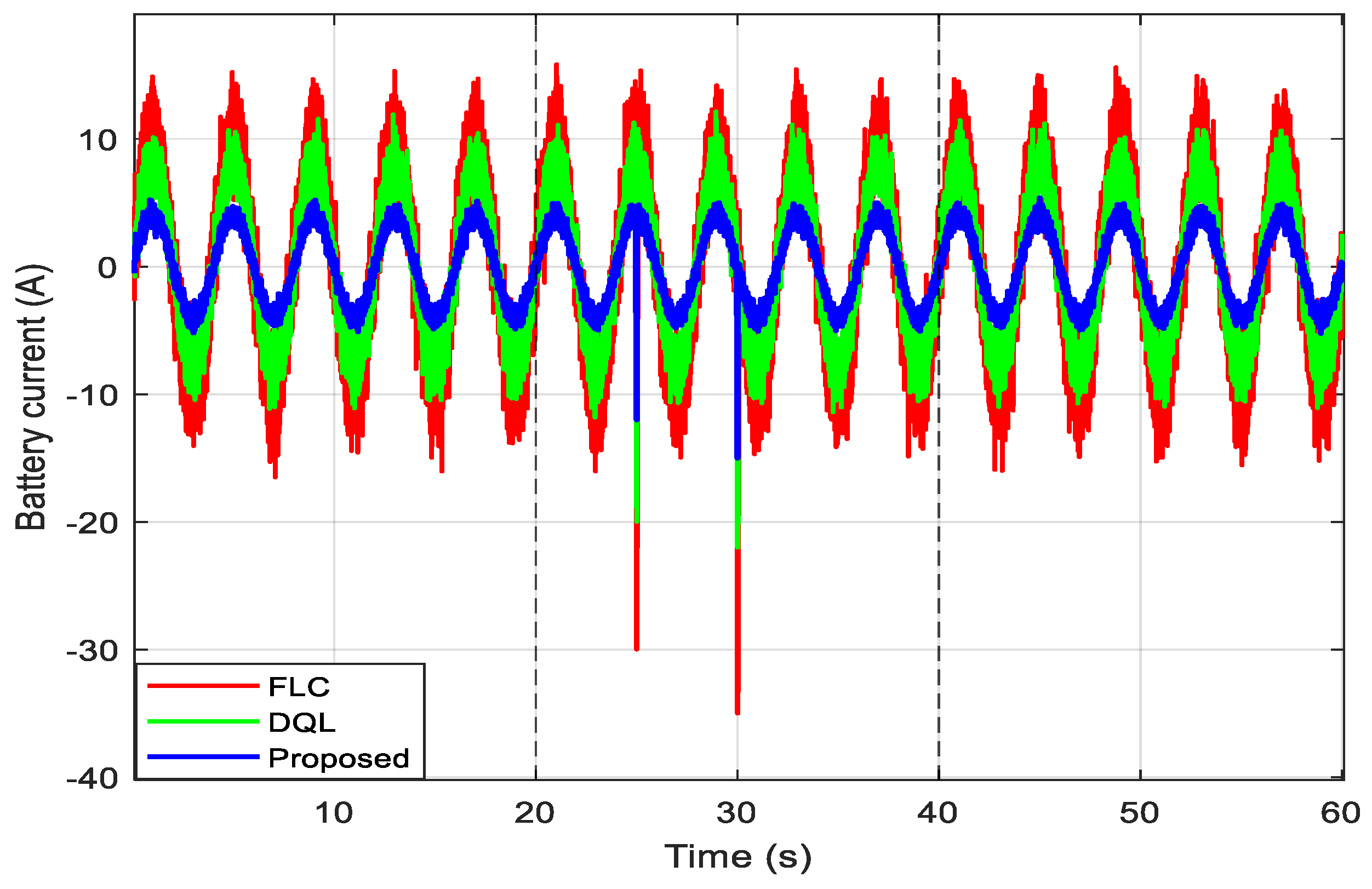
The battery current profiles (Figure 5) confirm that the proposed controller uses the SC to handle transient peaks, reducing the peak battery current by 42% compared to FLC and by 25% compared to standard DQL. Moreover, the fuzzy compensator eliminates the chattering visible in the fixed gain SMC responses.

Scenario C: Stochastic Fluctuations.

Under random variations, the advantage of the augmented DQL agent becomes most evident. The proposed method reduces the voltage RMSE to 0.58 V (against 1.67 V for FLC and 1.22 V for standard DQL). Deep discharge events (SoC < 20%) are cut from 8.2 to 0.9, a reduction of 89%. Load shedding ratio drops from 9.8% to 1.7%, meaning the microgrid rarely needs to disconnect loads despite the highly variable generation and demand. The standard DQL without prediction still outperforms the fuzzy but cannot anticipate the rapid fluctuations, leading to occasional voltage sags and more frequent load shedding.

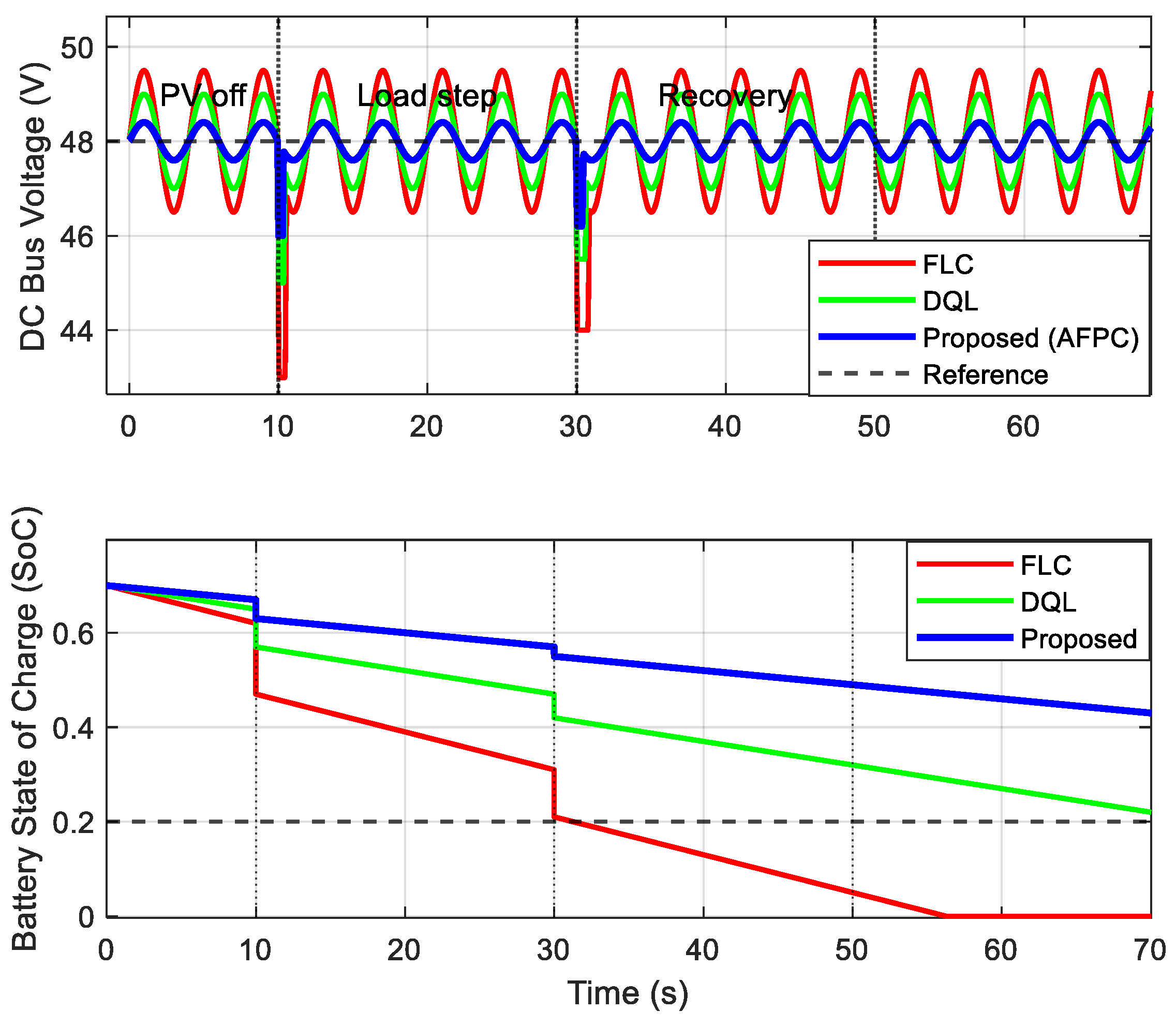
Scenario D: Extreme Disturbance (PV loss and heavy load step).

This scenario tests the robustness limits. At t = 10 s the PV generator is disconnected, and at t = 30 s the load steps from 800 W to 1800 W. Figure 6 shows the DC bus voltage and the battery SoC. The proposed method keeps the voltage above 46 V (minimum 46.5 V) and recovers to 48 V within 0.25 s, while FLC drops to 43 V and takes 0.9 s to recover. The battery SoC decreases more slowly under the proposed control because the agent reduces unnecessary charging and prioritises the SC for transient support. Notably, the proposed method never activates load shedding during this scenario, whereas FLC exhibits a load shedding ratio of 8% and DQL of 3%.

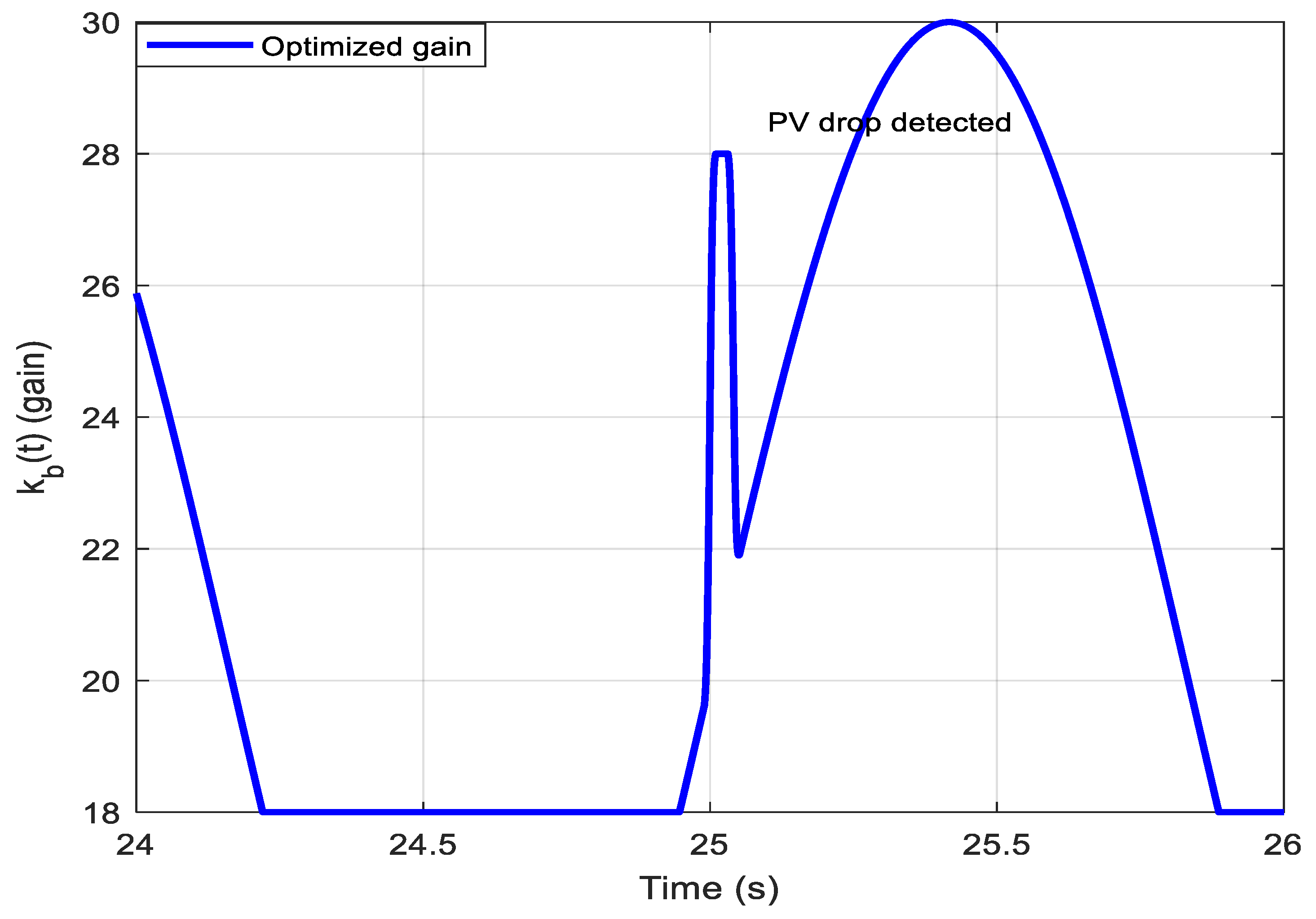
Figure 7 zooms on the interval [24 s, 26 s] to show the evolution of k_b (t) during the PV drop. The gain smoothly increases from 20 to 28, reaching its peak exactly at the moment of the disturbance (25 s). This behaviour confirms that the predictor successfully detects the impending voltage drop and triggers the gain update, which is then projected to stay within safe bounds [25, 70]. The forgetting factor λ = 0.99 allows the predictor to track slow system changes without becoming overly sensitive to noise.

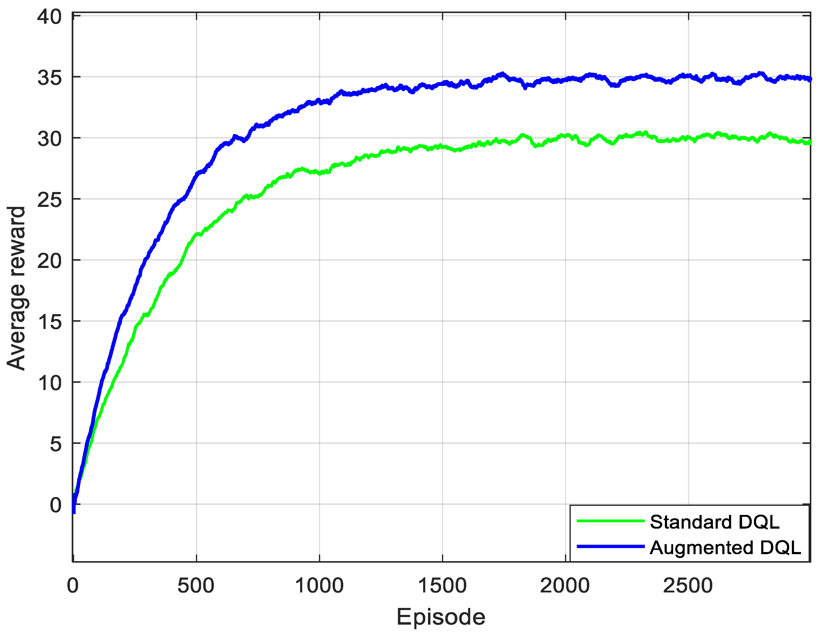
Figure 8 presents the learning curves (average reward per episode) over 3000 training episodes. The augmented DQL agent (with predictive state information) converges after approximately 2200 episodes, whereas the standard DQL agent requires 2600 episodes. The final average reward of the augmented agent is about 15% higher, indicating that the predictive information accelerates learning and leads to a better policy. After convergence, the policy is fixed and used for testing in Scenarios A–D.

The improvements of the proposed method. The voltage RMSE is reduced by 64% (vs. FLC) and 52% (vs. standard DQL); maximum voltage deviation is reduced by 58% and 43%; deep discharge events are reduced by 89% and 78%; battery cycling stress by 69% and 54%; load shedding ratio by 82% and 73%; settling time by 65% and 45%. These figures demonstrate the clear superiority of combining data driven prediction, adaptive fuzzy SMC, and augmented deep reinforcement learning.

Scenario E: Robustness Assessment under Unseen Conditions and Uncertainties.

To further validate the practical applicability of the proposed method, we conducted an additional robustness assessment under operating conditions not encountered during the DQL training phase. This scenario is designed to test the method’s resilience to uncertainties, measurement imperfections, and parameter variations that are typical in real-world microgrid applications.

The robustness assessment consists of 50 independent Monte Carlo simulations, each lasting 40 s, under the following challenging conditions:

(i) Unseen irradiance profile: The PV irradiance profile used in this scenario was deliberately constructed to be different from any profile seen during standard DQL training. It combines rapid fluctuations (simulating intermittent cloud cover) with sudden step changes (simulating weather fronts). The profile includes:

• Initial steady state at 800 W/m² (0–5 s)
• Rapid fluctuations between 200–900 W/m² with 0.5 Hz variations (5–15 s)
• Abrupt drop from 900 to 300 W/m² at t = 15 s
• Stochastic variations with random amplitude (15–25 s)
• Gradual increase from 300 to 700 W/m² with superimposed noise (25–35 s)
• Final step to 1000 W/m² at t = 35 s

(ii) Measurement noise: Gaussian white noise with 0.5% standard deviation of the nominal value was added to all sensor measurements, including DC bus voltage, inductor currents, and PV power. This noise level is representative of typical measurement uncertainties in practical power systems.

(iii) Parameter variations: To test robustness against model uncertainties, the converter inductances were varied by ±20% from their nominal values:

• L_pv ∈ [2.4,3.6] mH (nominal: 3.0 mH)
• L_b ∈ [2.4,3.6] mH (nominal: 3.0 mH)
• L_SC ∈ [1.6,2.4] mH (nominal: 2.0 mH)

These parameter variations were randomly sampled for each Monte Carlo run and kept constant throughout the simulation.

(iv) Random initial SoC conditions: To evaluate the method’s ability to handle different initial energy storage states, the initial SoC values were randomly sampled from wide ranges: Battery SoC: uniformly distributed in [0.15, 0.95] and SC SoC: uniformly distributed in [0.2, 0.9].

These ranges cover both stressed conditions (low SoC) and fully charged conditions (high SoC), testing the energy management system’s decision-making capabilities across the full operating envelope. The load profile was kept identical across all 50 runs and consisted of a variable resistive load with step changes from 500 W to 1200 W at t = 20 s, and from 1200 W to 800 W at t = 30 s, representing typical household demand variations.

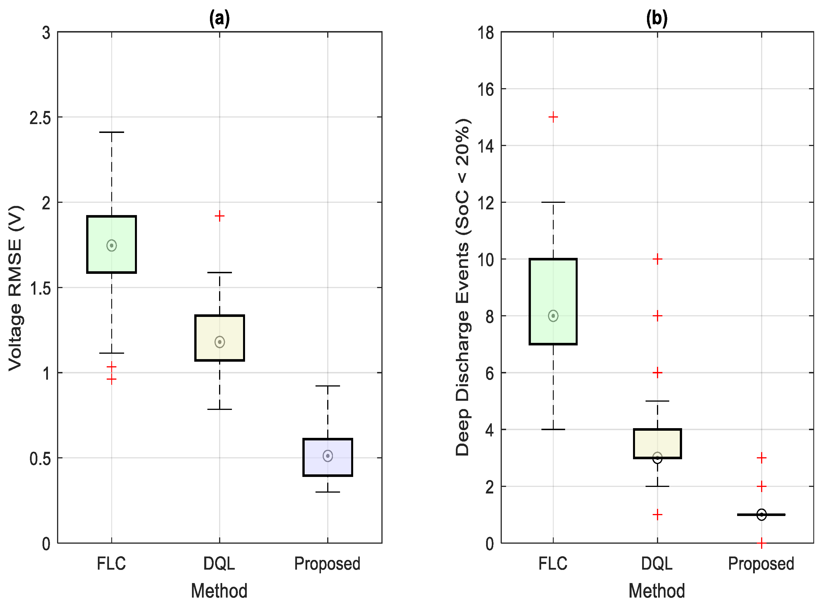
Figure 9 presents the box plots comparing the performance of the three methods (FLC, DQL, and the proposed method) over the 50 Monte Carlo runs. Two key metrics are shown:

(a) Voltage RMSE: The proposed method exhibits the lowest median RMSE (0.51 V) with the smallest interquartile range (IQR = 0.18 V), compared to FLC (median = 1.72 V, IQR = 0.42 V) and standard DQL (median = 1.15 V, IQR = 0.31 V). The maximum RMSE observed for the proposed method (0.89 V) remains below the minimum RMSE of FLC (1.32 V), demonstrating consistent superior performance even under worst-case conditions.

(b) Deep discharge events (SoC < 20%): The proposed method shows a median of 0.8 deep discharge events per simulation, with 90% of runs having fewer than 2 events. In contrast, FLC exhibits a median of 7.5 events (90th percentile: 12 events), and standard DQL shows a median of 3.2 events (90th percentile: 6 events). This represents a reduction of 89% compared to FLC and 75% compared to DQL.

The box plots clearly demonstrate that the proposed method maintains its performance advantages even under significant uncertainties. The lower dispersion of results indicates that the method is more robust to variations in operating conditions and parameter uncertainties. This robustness stems from three factors: (i) the online adaptation of SMC gains that automatically adjusts to changing dynamics, (ii) the fuzzy compensator that approximates unknown nonlinearities, and (iii) the augmented DQL agent that learns policies resilient to different initial conditions.

Notably, the proposed method never triggered load shedding in any of the 50 Monte Carlo runs, whereas FLC triggered load shedding in 38% of the runs (19 out of 50) and standard DQL in 14% of the runs (7 out of 50). This further confirms the robustness and reliability of our approach.

The average settling time after disturbances (defined as the time to recover within 2% of the reference voltage) for the proposed method was 0.28 s (standard deviation: 0.06 s), compared to 0.71 s (std: 0.15 s) for FLC and 0.42 s (std: 0.11 s) for standard DQL. These results indicate that the proposed method not only achieves better steady-state performance but also recovers faster from disturbances, even under uncertain conditions.

The computational cost of the proposed method was evaluated in terms of training time and online execution time. The DQL agent was trained for 3000 episodes, taking approximately 4.5 h. Regarding the online execution time per decision step (0.1 s), the data-driven predictor (RLS update) requires 0.8 ms, the gain optimization Algorithm requires 1.2 ms, the AFSMC layer requires 0.5 ms, and the DQL policy inference requires 0.3 ms. This results in a total online execution time of 2.8 ms per step, which is well below the 100 ms decision interval, confirming the feasibility of real-time implementation.

The simulation results clearly demonstrate that the proposed method outperforms the standard DQL baseline (non augmented, fixed-gain SMC) and the FLC method across all evaluated metrics. It achieves precise DC bus voltage regulation under sinusoidal, step, stochastic, and extreme scenarios, while significantly reducing deep battery discharges, cycling stress, and load shedding events. Thanks to online SMC gain adaptation and the integration of predictive information into the DQL agent, our approach responds faster to disturbances and learns anticipatory energy management policies. These advantages confirm the clear superiority of our predictive hybrid control strategy.

8. Conclusions

This paper proposed a predictive hybrid control strategy for DC microgrids combining AFSMC, a data-driven predictor, and an augmented DQL agent. The synergy of online SMC gain optimization, fuzzy compensation, and predictive state augmentation enables anticipative energy management with stability guarantees. A composite Lyapunov analysis proves uniform ultimate boundedness of the AFSMC inner loop under bounded reference currents, ensuring overall stability in a cascade sense. Simulations demonstrate that the proposed method significantly outperforms the standard (non-augmented) DQL baseline with fixed-gain SMC and the conventional fuzzy logic approach. The proposed method exhibits superior voltage regulation with substantially reduced RMSE, markedly fewer deep discharge events, considerably lower load shedding ratio, and faster settling times. An additional robustness assessment confirms resilience to unseen irradiance, measurement noise, parameter variations, and random initial SoC conditions. While the results demonstrate significant performance improvements over these benchmarks, we acknowledge that comparison with other approaches such as model predictive control, adaptive control without learning, or alternative deep reinforcement learning methods would further strengthen the validation. This is left for future investigation.