Article

Convergence-to-Zero and Guaranteed-Cost Synchronization of Caputo–Hadamard Fractional-Order Systems with a Time-Varying Delay

1
Department of Mathematics, College of Science, Jouf University, P.O. Box 2014, Sakaka 72388, Saudi Arabia
2
Department of Computer Engineering and Networks, College of Computer and Information Sciences, Jouf University, Sakaka 72341, Saudi Arabia
3
Department of Mathematics, College of Science, King Khalid University, Abha 61413, Saudi Arabia
*
Author to whom correspondence should be addressed.
Mathematics 2026, 14(15), 2788; https://doi.org/10.3390/math14152788
Submission received: 2 July 2026 / Revised: 28 July 2026 / Accepted: 30 July 2026 / Published: 4 August 2026
(This article belongs to the Special Issue Advances in Fractional Differential Equations and Applications)

Abstract

In this paper, the convergence-to-zero and finite-horizon guaranteed-cost synchronization criteria are developed for linear Caputo–Hadamard fractional-order systems with an admissible time-varying delay. The delay assumption is expressed in such a way that is consistent with the Caputo–Hadamard Halanay inequality and the memory structure of the model, which is logarithmic in time. This analysis includes a quadratic Caputo–Hadamard Lyapunov method, Schur-complement bounds for the delayed channel and a supremum argument in logarithmic time. An important novelty in the proposed approach is that the current state, the delayed state and the Caputo–Hadamard derivative are not considered as independent augmented variables; this prevents the structural feasibility obstacle from occurring when using full-space residual LMI formulations. The convergence-to-zero condition is first established for the drive system. Next, a fixed-gain guaranteed-cost synchronization theorem is established and, by using a standard change of variables, a convex controller-synthesis condition is arrived at. An explicit logarithmic-time form of the finite-horizon cost estimate is derived. The criteria are further extended to systems with several admissible delays and to systems with norm-bounded parametric uncertainty. Four numerical examples are reported, in which feasible matrices, the controller gain, strict eigenvalue margins and a comparison of the simulated cost and the theoretical upper bound are given, together with a quantitative comparison against augmented-state linear matrix inequality formulations, a scalability study up to a dimension of 30 and a sensitivity study. The simulations show the dynamics that the theory predicts; the convergence to the asymptotics is valid for the LMI certificates checked in the simulations and for the Caputo–Hadamard Halanay inequality. In conclusion, the paper delivers a complete and numerically verifiable design chain for Caputo–Hadamard synchronization: admissibility of a possibly unbounded time-varying delay is checked directly, a stabilizing gain is obtained from a convex program whose largest block has size 2 n instead of 3 n , and an a priori cost certificate J T * is produced from the same feasible variables; on the reported benchmark, the method retains 95.7 % of the admissible delay-channel gain of an augmented-state formulation while solving up to 21 times faster at dimension 30.

1. Introduction

Fractional-order (FODS) dynamic systems have emerged as a significant modelling tool for phenomena that display memory, hereditary effects, nonlocal damping and anomalous transient behaviours. The analytical aspects of fractional differential equations such as the existence theory, integral representations, qualitative properties of fractional operators have been studied in classical monographs and foundational studies [1]. The Hadamard and Caputo–Hadamard derivatives are of particular interest among the various types of fractional derivatives, particularly in the description of the memory on a logarithmic scale and not linear scale. The Caputo-type modification of the Hadamard derivative is useful for the physical problem, which has several physically meaningful initial conditions, and some papers have been devoted to uncovering the basic properties of this modification, equivalent integral forms, and connections with Hadamard-type fractional calculus [2,3,4].
Several inequivalent fractional derivatives are available—Riemann–Liouville, Caputo, Hadamard, Caputo–Hadamard, conformable, and tempered and variable-order operators among them—and the choice is dictated by the memory law that the application requires rather than by mathematical convenience. Three properties single out the Caputo–Hadamard operator for the present study. First, its kernel ( ln ( t / s ) ) ς 1 weights the past on a logarithmic clock, so that the induced relaxation is ultraslow (logarithmic) rather than the power-law relaxation produced by the Riemann–Liouville and Caputo kernels; this is the correct law for ageing and creep in viscoelastic solids and geomaterials, for ultraslow diffusion in strongly disordered media, and for long-horizon drift and fatigue phenomena in which the effective memory horizon grows multiplicatively with elapsed time. Second, in contrast with the Riemann–Liouville–Hadamard derivative, the Caputo modification is compatible with classical, physically measurable initial data x ( a ) = x a rather than with initial values of a fractional integral, which is what makes an initial-condition-dependent cost certificate such as Equation (37) meaningful in the first place. Third, the operator has already proved to be the appropriate modelling device in concrete engineering settings: data-driven variable-order Caputo–Hadamard control has been validated on power-system resilience data [5], and Caputo–Hadamard formulations have been used for coupled fuzzy fractional systems [6] and for reaction–diffusion dynamics [7]. On the control side, the synchronization problem treated here with an explicit performance certificate is the abstraction of master–slave teleoperation, chaos-based secure communication, clock and phase alignment in distributed sensor networks, and coupled-converter synchronization in power electronics; in all of these, the designer needs both a convergence guarantee and an a priori bound on accumulated control and tracking effort, which is exactly what a guaranteed-cost formulation provides. The starting instant a > 0 required by the Hadamard kernel is not a restriction in these applications, since it simply fixes the instant from which the logarithmic clock is measured.
The analysis of stability of fractional order systems is very distinct from integer order systems. Notably, Lyapunov methods should take into consideration the nonlocal nature of the fractional derivative and the particular type of decay brought about by the fractional kernel used. Fractional systems require a solid foundation for this purpose, and it is given by general Lyapunov-type inequalities [8]. The logarithmic-time structure of Caputo–Hadamard systems gives rise to certain comparison arguments and Halanay-type estimates which are well adapted to systems with delayed dynamics [9]. In recent years, the stability, finite-time stability, stochastic stability and uncertainty analysis of Hadamard and Caputo–Hadamard fractional systems were studied in further details, which further demonstrates the growing interest in this kind of fractional systems (see [10,11,12]). For neutral systems and stochastic delay equations with Hadamard type operators, there are also related stochastic and delay dependent formulations that have been studied in [13,14,15].
Another important source of complexity of nonlinear dynamical systems are time delays. Delays can play a crucial role in the convergence, boundedness and synchronization behaviour, and are coupled to the memory kernel in fractional-order models. In the case of Caputo–Hadamard systems this interaction is even more fragile as the effective memory is changing in accordance with the logarithmic clock. Delayed fuzzy Hadamard fractional order systems, Caputo–Hadamard fractional order neural network with time varying delays and output feedback synchronization of uncertain nonlinear Caputo–Hadamard systems were recently treated in [16,17,18], respectively. Some other synchronization conditions are given for the Caputo–Hadamard competitive neural networks with discrete, distributed and time-varying delays in [19,20], respectively. These studies show that the topic of delay-dependent synchronization of Caputo–Hadamard systems is a timely and mathematically challenging one.
Synchronization is a key issue of complex dynamical networks, neural systems, physical oscillators, cyber-physical systems and engineering applications. Synchronization and delay synchronization has been studied in various contexts such as Kuramoto-oscillator networks, monitoring setups using IoT technology, adaptive blinking coupling networks, and low-cost educational experiments for complex systems [21,22,23]. Generalized network synchronization strategies have also been developed to cope with the effect of topology and time-varying coupling mechanisms [24]. In fractional order setting, the phenomenon of synchronization is of particular interest since fractional dynamics can model long memory effects which are not captured in classical integer order models. The relevance of the memory-dependent dynamics is further highlighted by high-dimensional fractional neural networks, fractional deterministic learning, and fractional learning algorithms, in control, identification, and learning problems, respectively, discussed in [25,26,27].
The fractional-order literature that is directly relevant to the present contribution extends well beyond the Caputo–Hadamard class. Sliding-mode designs have been used to obtain finite-time synchronization of uncertain fractional-order delayed memristive neural networks together with a secure-communication application [28], which is the closest existing counterpart to the synchronization objective considered here, although the settling-time argument used there requires a bounded delay and a discontinuous control law. Consensus of nonlinear fractional-order multi-agent systems with diffusion has been achieved by adaptive fault-tolerant protocols [29], an application in which a guaranteed-cost certificate of the type derived below would be directly useful. On the analytical side, the solvability theory of fractional boundary-value problems provides the well-posedness background for fractional models: the existence and uniqueness of positive solutions of fractional differential systems on infinite intervals were established in [30], and the solvability of nonlinear fractional boundary-value problems with mixed perturbations of the second type was obtained in [31]. Fractional-order modelling has also proved effective in the life sciences, for tumour–immune interaction [32] and for prey–predator dynamics with hunting cooperation and gestation delay [33], the latter being a further instance in which a fractional operator and a time delay act simultaneously. These works confirm both the breadth of fractional-order dynamics and the fact that the combination of delay, convex synthesis and an a priori performance certificate that we address here has not been settled in the Caputo–Hadamard setting.
In nonlinear fractional order systems, observer-based control and synchronization are still a challenge as together with fractional memory, the nonlinearities and uncertain parameters need to be addressed. In recent years, several works have been proposed for the observer and controller design of nonlinear Hadamard fractional-order systems, such as one-sided Lipschitz methods [34] and sum-of-squares-based approaches [35]. The convergence of modern fractional and nonlinear control is increasingly moving towards merging analytic stability conditions and computational design procedures. This trend is illustrated by three closely related lines of work. In [36], a hierarchical neural identification scheme is developed for Hammerstein large-scale stochastic systems and validated on a hydraulic process, showing how a data-driven model can be extracted before any certificate is computed. In [37], a data-driven certified mode-detection procedure is proposed for switched discrete-time Takagi–Sugeno systems with an adaptive observation window, so that the identified mode carries a verifiable guarantee rather than a heuristic score. In [38], a gradient-based optimization algorithm is designed for optimal control problems governed by general conformable fractional derivatives, which is the optimization counterpart of the convex synthesis step used in the present paper. Taken together, [36,37,38] show that identification, certification and fractional optimal control are converging towards numerically checkable design procedures, which is precisely the standard adopted here. These advances create a need to find tractable synchronization conditions that are amenable to numerical verification and can be used to design and implement synchronization via convex optimization techniques.
Linear matrix inequalities are a powerful and efficient way for stability and control synthesis. The LMI methodology has been used extensively to establish numerically verifiable feasibility problems from Lyapunov inequalities [39] and has become a common technique for robust control. For the fractional order systems with delays, LMI-based conditions have specific advantage, as they can simultaneously handle controller gains, Lyapunov matrices, delay parameters and performance constraints. Guaranteed-cost synchronization is an important extension of stabilization and synchronization, since it can not only guarantee convergence, but also explicitly bound an accumulated performance index. Recently, the admissible Mittag–Leffler stability and guaranteed-cost synchronization for fractional-order singular systems with multiple time-varying delays were studied, which demonstrate the significance of synergizing the synchronization analysis with performance guarantees [40].
Although all of the above progress has been made, there are still some limitations. First, the many synchronization results for Caputo–Hadamard systems are in the context of Mittag–Leffler-type estimates or finite-time boundedness, while reaching convergence to zero with respect to admissible time varying delay requires a careful logarithmic-time study. Second, some of the current methods are based on the augmented-state or conservative delay techniques, which do not necessarily show the specific Caputo–Hadamard structure. Third, guaranteed-cost synchronization of Caputo–Hadamard systems with time-varying delay is not as well developed as that of integer-order or classical Caputo systems. Fourth, not all of the theoretical matrix inequalities are strictly feasible, and sometimes, numerical examples only show convergence by plotting, while not verifying the strict feasibility of the matrix inequalities. These points motivate a framework that connects convergence analysis, controller synthesis, and verifiable certificates of performance over finite horizons, all tied to LMIs.
The contribution of the paper with respect to the existing Caputo–Hadamard synchronization literature can be stated precisely as follows.
(C1)
Delay class. Convergence to zero of the synchronization error is obtained under exactly the admissibility class of the logarithmic Halanay inequality, namely 0 ϖ ( t ) t a with t ϖ ( t ) . This class contains unbounded delays such as ϖ ( t ) = ( 1 c ) ( t a ) , c ( 0 , 1 ) , and is therefore strictly larger than the bounded-delay class ϖ ( t ) h with a prescribed history on [ a h , a ] used in [17,18,19,20]. Section 4.2 exhibits an admissible delay that grows without bound.
(C2)
Removal of a structural obstruction. Proposition 2 proves that the full-space residual LMI written on the augmented vector col { e ( t ) , e ( t ϖ ( t ) ) , D a ς C H e ( t ) } can never be negative definite, because the block associated with D a ς C H e vanishes identically. The delay-channel Schur estimate used here removes this obstruction rather than working around it numerically.
(C3)
Explicit logarithmic-time cost certificate. The guaranteed cost is delivered in closed form, J T * = V a + β e V ¯ ( ln ( T / a ) ) ς / Γ ( ς + 1 ) , computable from the initial error and the feasible LMI variables alone. Proposition 1 additionally supplies a conditional infinite-horizon bound under an extra Mittag–Leffler decay hypothesis, which clarifies exactly what is missing for an infinite-horizon statement.
(C4)
Quantified conservatism and cost. The largest LMI block produced by the proposed synthesis has size 2 n instead of the 3 n block of augmented-state formulations. Section 4.5 shows on the benchmark of Section 4 that this costs 4.29 % of admissible delay-channel gain relative to a free-weighting augmented-state analysis while reducing the number of decision variables from 3165 to 930 and the solver time from 4835 ms to 227 ms at n = 30 .
(C5)
Extensions and certificate-based validation. Theorem 4 extends the synthesis to q simultaneous admissible delays and Theorem 5 to norm-bounded parametric uncertainty in both A and A d . Four numerical examples report strict eigenvalue margins, solver settings and timings, so that every hypothesis used in the proofs is verified numerically rather than inferred from a trajectory plot.
Table 1 positions the paper against representative recent works on Caputo–Hadamard and fractional-order synchronization.
In this paper, a guaranteed-cost synchronization framework for linear Caputo–Hadamard fractional-order systems with time-varying delay is developed based on the LMI approach. The analysis proposed in the paper takes advantage of the logarithmic-time nature of the Caputo–Hadamard derivative and establishes delay-admissible conditions for the convergence to zero of the drive dynamics and synchronization error. The state-feedback synchronization controller is designed based on convex LMI conditions, and a fixed-gain verification step is given to verify the recovered controller. Moreover, a finite-horizon guaranteed-cost estimate is obtained, which provides an explicit upper bound of the synchronization performance index that can be computed. The numerical example is created and not only depicted graphically, but also directly verified with the theory: the admissibility of the delay is verified, the corresponding matrices in the LMI are calculated, explicit eigenvalue margins are computed, and the cost is simulated and compared with the theoretical bound. Predictor–corrector discretization ideas are applied uniformly to the fractional dynamics for the numerical integration of the fractional dynamics, which is consistent with the common numerical methods for fractional differential equations [41]. The relevance of such fractional control frameworks, which can be verified computationally, was further illustrated in recent applications to include the use of variable-order fractional control [5], fuzzy fractional coupled systems [6] and more general Caputo–Hadamard modelling [7].
The scope of the paper is deliberately restricted to linear drive–response pairs with a finite number of discrete admissible delays, and the restriction is a modelling choice rather than an oversight. Linearity is what makes the delay-channel estimate (25) lossless in the sense of Corollary 1, and it is what allows the change of variables W = P 1 , Y = K W to convexify the synthesis exactly; for Lipschitz or one-sided Lipschitz nonlinearities, an additional scaling parameter must be introduced and the resulting condition is no longer tight. Likewise, the single quadratic Lyapunov function V e = 1 2 e T P e used throughout does not carry any delay-dependent term, so the criteria obtained here are delay-rate independent: they hold for every admissible ϖ , but they cannot exploit knowledge of a small delay bound to enlarge the feasible set. Section 3.5 removes the single-delay restriction, Section 3.6 removes the exact-model restriction, and Section 5 lists what remains open.
The rest of this paper will be arranged as follows. In Section 2, the definitions, inequalities and auxiliary results, which are required in the sequel, are recalled for Caputo–Hadamard fractional systems with time-varying delays. The convergence analysis, the conditions for controller synthesis based on the LMI approach and the estimate of finite-horizon cost are presented in Section 3, together with the extensions to several delays (Section 3.5) and to norm-bounded uncertainty (Section 3.6). Four detailed numerical examples, a quantitative comparison with augmented-state formulations, a scalability study and a sensitivity study are presented in Section 4. Finally, Section 5 concludes the paper and provides some suggestions for future research.

2. Preliminaries and Problem Formulation

Throughout this paper, R n denotes the n-dimensional Euclidean space, and R n × m denotes the set of real matrices of dimension n × m . For a matrix M, M T denotes its transpose. If  M = M T , then M > 0 and M < 0 mean that M is positive definite and negative definite, respectively. The notation ∗ denotes symmetric block entries. For a symmetric matrix M, λ min ( M ) and λ max ( M ) denote its smallest and largest eigenvalues. The Euclidean norm of a vector and the induced spectral norm of a matrix are denoted by · . We write sym ( M ) = M + M T . For a symmetric positive-definite M, M 1 / 2 denotes its unique symmetric positive-definite square root, and  I k is the k × k identity matrix. The Hadamard fractional integral operator of order ς with base point a is written I a ς and the Caputo–Hadamard derivative D a ς C H ; when the derivative acts on a function of the running variable s, this is made explicit by writing D a ς C H V ( s ) , with the subscript a always denoting the base point of the operator and s the variable of differentiation. Vectors carrying the subscript a, namely x a , y a and e a , are the initial-condition vectors  x ( a ) , y ( a ) and e ( a ) = x a y a prescribed at the initial instant t = a ; they are constant vectors of R n and are never fractional integrals. Table 2 collects the symbols that are used repeatedly.
Let a > 0 and 0 < ς < 1 be fixed.
Definition 1 
(Hadamard fractional integral [1,2]). Let g be locally integrable on [ a , ) . The Hadamard fractional integral of order ς is
I a ς g ( t ) = 1 Γ ( ς ) a t ln t s ς 1 g ( s ) d s s , t a .
Definition 2 
(Caputo–Hadamard fractional derivative [2,3]). Let h be absolutely continuous on every compact subinterval of [ a , ) . The Caputo–Hadamard derivative of order ς is
D a ς C H h ( t ) = 1 Γ ( 1 ς ) a t ln t s ς h ( s ) d s , t > a .
The following quoted results are used as tools. Each lemma in this preliminary section is cited explicitly; the proofs are not reproduced here.
Lemma 1 
(Quadratic Caputo–Hadamard inequality [8,9]). Let ς be a real number satisfying 0 < ς < 1 , and let S be a symmetric positive definite matrix in R n × n . Then, for every σ t 0 ,
D t 0 ς C H 1 2 x ( σ ) T S x ( σ ) D t 0 ς C H x ( σ ) T S x ( σ ) .
Remark 1 
(On the restriction 0 < ς < 1 in Lemma 1). The restriction 0 < ς < 1 is not a technical convenience; it is what makes the whole chain of arguments of this paper available, for three independent reasons. (i) Definition. The Caputo–Hadamard derivative in Equation (2) is defined for 0 < ς < 1 through a single differentiation h under the kernel ( ln ( t / s ) ) ς . For  ς 1 , one must use the higher-order operator δ m , δ = t d / d t , with  m = ς , which requires m initial conditions δ k x ( a ) , k = 0 , , m 1 , and destroys the one-to-one correspondence between the single initial vector x a and the certificate V a = 1 2 e a T P e a on which the cost bound in Equation (37) rests. (ii)  Proof of the inequality. The proof of Equation (3) rests on the positivity of the kernel ( ln ( t / s ) ) ς together with the fact that the remainder produced by integration by parts, which is proportional to ς ( 1 ς ) -weighted differences, keeps a fixed sign exactly when ς ( 0 , 1 ) . For  ς > 1 , the corresponding quadratic estimate is known to fail in general. (iii) Comparison theory. The Caputo–Hadamard Halanay inequality of Lemma 2 is stated in [9] for ς ( 0 , 1 ) , and its proof uses the complete monotonicity of E ς ( λ θ ς ) and the nonnegativity of E ς , ς ( λ θ ς ) , both of which hold precisely on 0 < ς < 1 . (They fail for ς > 1 , where the Mittag–Leffler function oscillates and changes sign.) The same range is therefore imposed on the whole paper, and the identity I a ς ( D a ς C H V ) ( t ) = V ( t ) V ( a ) used in the cost estimate is likewise valid on this range only.
Lemma 2 
(Caputo–Hadamard Halanay inequality [9]). Let V : [ a , ) R + be continuous and Caputo–Hadamard differentiable on ( a , ) . Let τ : [ a , ) R + be continuous and satisfy
0 τ ( t ) t a , t τ ( t ) as t .
If there exist constants λ > μ > 0 such that
D a ς C H V ( t ) λ V ( t ) + μ sup τ ( t ) η 0 V ( t + η ) , t > a ,
then
lim t V ( t ) = 0 .
Lemma 3 
(Schur complement [39]). Let
M = M 11 M 12 M 22
be symmetric. If  M 22 < 0 , then M < 0 if and only if
M 11 M 12 M 22 1 M 12 T < 0 .
If M 22 > 0 , then M 0 if and only if
M 11 M 12 M 22 1 M 12 T 0 .

2.1. Single-Delay System

Consider the Caputo–Hadamard fractional-order system with one time-varying delay
D a ς C H x ( t ) = A x ( t ) + A d x ( t ϖ ( t ) ) , t > a , x ( a ) = x a ,
where x ( t ) R n , A , A d R n × n , and  x a R n is the initial-condition vector, that is, the value x ( a ) of the state at the initial instant t = a .
Assumption 1. 
The delay function ϖ : [ a , ) R + is continuous and satisfies
0 ϖ ( t ) t a , t ϖ ( t ) as t .
The condition ϖ ( t ) t a ensures that the delayed argument t ϖ ( t ) remains inside [ a , t ] . This is the delay structure required by Lemma 2. It is more restrictive than a generic bounded-history delay with a prescribed history on [ a h , a ] ; the present model is a Volterra-type retarded model in which the delayed argument remains in [ a , t ] . This restriction avoids applying the cited Halanay theorem outside its stated range. The condition t ϖ ( t ) also allows some unbounded delays, provided that the delayed argument still tends to infinity.
Remark 2 
(Interpretation and practical scope of Assumption 1). Assumption 1 has a direct interpretation on the logarithmic clock and a clear practical reading.
 (a) 
No pre-history is required. Because ϖ ( t ) t a , the delayed argument never leaves [ a , t ] , so the model is completely determined by the single vector x a . In practice, this means that the loop may be closed at the instant t = a at which the plant is switched on, without having to store, measure or postulate a history segment on [ a h , a ] . This is exactly the situation in start-up transients of master–slave links and in networked loops that are commissioned online.
 (b) 
Two admissible families. Every bounded continuous delay with ϖ ( t ) t a is admissible; this covers actuation and transmission lags that settle to a constant, such as ϖ ( t ) = h ( 1 e ( t a ) ) used in Section 4.1. In addition, all proportional (pantograph-type) delays ϖ ( t ) = ( 1 c ) ( t a ) with c ( 0 , 1 ) are admissible, since t ϖ ( t ) = a + c ( t a ) ; these describe sensing or communication lags that scale with elapsed operating time, as in accumulated-drift and ageing models. More generally ϖ ( t ) = ( t a ) ψ ( t ) is admissible whenever 0 ψ 1 and ( t a ) ( 1 ψ ( t ) ) , which admits ψ ( t ) 1 , that is, delays that asymptotically consume almost the whole history; Section 4.7 reports a simulation with ψ ( t ) = 1 1 / ln ( e + t ) .
 (c) 
What is excluded. Delays with t ϖ ( t ) are excluded. Take, for instance, ϖ ( t ) = t a κ with κ > 0 fixed. In this case, the delayed argument stalls near the fixed instant a + κ , and no attractivity conclusion is available from Lemma 2. No bound on ϖ ˙ is needed anywhere, so fast, non-differentiable and non-monotone delays are allowed.
 (d) 
Consequence for the design. Neither (17)–(18) nor (32)–(33) contains ϖ. The certificates are therefore uniform over the whole admissible class: one feasible solution certifies every admissible delay simultaneously. This is verified numerically in Section 4.7, where a single certificate is used for five different delay profiles, bounded and unbounded. The price is that a small delay bound cannot be exploited to enlarge the feasible set, which is the delay-rate-independent character discussed in Section 5.

2.2. Synchronization Model and Cost

The response system is
D a ς C H y ( t ) = A y ( t ) + A d y ( t ϖ ( t ) ) + B u ( t ) , t > a , y ( a ) = y a ,
where y ( t ) R n , u ( t ) R m , and  B R n × m . Define the synchronization error
e ( t ) = x ( t ) y ( t ) , e a = x a y a .
Then,
D a ς C H e ( t ) = A e ( t ) + A d e ( t ϖ ( t ) ) B u ( t ) , e ( a ) = e a .
We use the state feedback
u ( t ) = K e ( t ) ,
which gives the closed-loop error system
D a ς C H e ( t ) = A K e ( t ) + A d e ( t ϖ ( t ) ) , A K = A B K , e ( a ) = e a .
Remark 3 
(On the state-feedback law (11)).  The control in Equation (11) is a static, memoryless, full-error state feedback with constant gain K R m × n , and each of these four attributes is deliberate.
 (i) 
What is fed back. The signal e ( t ) = x ( t ) y ( t ) is the instantaneous synchronization error between the drive and the response state. In a master–slave implementation, the drive state x ( t ) is transmitted to the response unit, which measures its own state y ( t ) and forms e ( t ) locally; only the current value is needed. The signal u ( t ) = K e ( t ) is injected in the response system in Equation (9) through B; hence, it enters the error dynamics in Equation (10) with the opposite sign, which is why the closed-loop matrix is A K = A B K and not A + B K .
 (ii) 
Why it is memoryless. No delayed term K d e ( t ϖ ( t ) ) and no distributed term are used. A delayed feedback would require on-line knowledge of ϖ ( t ) , which is not assumed anywhere: Assumption 1 only constrains ϖ qualitatively and permits unbounded, non-differentiable delays. A memoryless law is therefore the only implementable structure that is uniform over the whole admissible class, and it is what makes the design delay-rate independent.
 (iii) 
Why the gain is constant. A constant K keeps the closed-loop error system in Equation (12) linear and time-invariant apart from the delayed argument, which is what allows the quadratic Lyapunov function in Equation (21) to produce the scalar Halanay inequality in Equation (48) with constant coefficients α e , β e , hence to invoke Lemma 2 directly. Time-varying or adaptive gains would require a comparison theorem with time-varying rates, which is not available in the Caputo–Hadamard setting.
 (iv) 
Why it convexifies. Substituting Equation (11) into the cost density in Equation (14) makes the control penalty u T R u = e T K T R K e quadratic in e with the coefficient K T R K ; the product terms P B K and K T R K that appear in Equation (32) are then linearized exactly by W = P 1 , Y = K W , giving the convex condition in Equation (55). No such exact linearization is available for output feedback u = K o C e with a prescribed C, which is why the present paper treats the full-error case, and [18] treats the output-feedback case by a different route.
Finally, m need not equal n: Section 4.3 uses n = 4 states and m = 2 inputs, so that the design is not restricted to fully actuated systems.
Definition 3 
(Convergence synchronization; cf. [18] (Def. 2.1), [17] (Def. 2), [40] (Def. 3.1)). The drive system in Equation (7) and the response system in Equation (9) achieve convergence synchronization under Equation (11) if
lim t e ( t ) = 0 .
Definition 4 
(Finite-horizon guaranteed-cost convergence synchronization; adapted from the guaranteed-cost notions of [40] (Def. 3.2) and [39] (Ch. 7)). For a given T > a , the feedback law in Equation (11) achieves finite-horizon guaranteed-cost convergence synchronization if it achieves convergence synchronization and provides an a priori computable constant J T * > 0 , depending only on the initial error, the horizon, and the feasible design variables, such that
J ( t ) J T * , a t T .
The two notions above are the Caputo–Hadamard counterparts of standard definitions in the fractional synchronization literature. Definition 3 is the attractivity form of synchronization used for Caputo–Hadamard systems in [17,18,19]; it is weaker than Mittag–Leffler synchronization because no decay rate is asserted, and Section 2.3 explains why the weaker form is the sharp one in the admissible delay class of Assumption 1. Definition 4 follows the classical guaranteed-cost paradigm of [39] (Ch. 7), in which a stabilizing controller is required to come with an a priori bound on a quadratic performance index, transposed to the fractional cost in Equation (13); the same paradigm is used in the fractional singular setting of [40] (Def. 3.2), the difference being that the bound is asserted there on an infinite horizon under a Mittag–Leffler estimate, whereas here it is asserted on a finite horizon under attractivity only.
Let S = S T > 0 , S d = S d T > 0 , and  R = R T > 0 . For a prescribed finite horizon T > a , define the finite-horizon guaranteed-cost functional
J ( t ) = 1 Γ ( ς ) a t ln t s ς 1 ( s ) d s s , a t T ,
where
( t ) = e T ( t ) S e ( t ) + e T ( t ϖ ( t ) ) S d e ( t ϖ ( t ) ) + u T ( t ) R u ( t ) .
Remark 4. 
The cost bound is stated on a finite horizon because Lemma 2 yields convergence to zero without a decay rate, and an infinite-horizon bound cannot be obtained from attractivity alone. Proposition 1 below makes precise the additional hypothesis under which the horizon can be sent to infinity.

2.3. Why Convergence to Zero, and What an Infinite Horizon Would Require

It is natural to ask why the convergence-to-zero framework is adopted here instead of the Mittag–Leffler stability framework that prevails in much of the fractional synchronization literature [17,19,40]. The reason is the delay class. A Mittag–Leffler estimate of the form V e ( t ) c V a E ς ( λ ( ln ( t / a ) ) ς ) is available for Caputo–Hadamard systems when the delay is bounded and a history segment is prescribed, but no such estimate is known—and none is claimed here—for the full admissible class 0 ϖ ( t ) t a , t ϖ ( t ) , which contains delays that asymptotically consume almost the entire history. In that class the sharp conclusion supplied by the logarithmic Halanay comparison of [9] is attractivity, and stating a rate would require assumptions that Assumption 1 deliberately does not make. Adopting convergence to zero is thus a way of buying a strictly larger delay class at the price of a rate, and the finite-horizon form of the cost certificate is the exact accounting entry for that trade. The following proposition shows that the trade is reversible: as soon as a Mittag–Leffler decay is available, the same feasible variables deliver an infinite-horizon bound with no further design effort.
Proposition 1 
(Conditional infinite-horizon cost bound). Let the hypotheses of Theorem 2 hold, and assume in addition that
 (H1) 
There exist c 1 and λ > 0 such that V e ( t ) c V a E ς λ ln t a ς for all t a ;
 (H2) 
There exists c 0 ( 0 , 1 ] such that ln t ϖ ( t ) a c 0 ln t a for all t a .
Then, with  κ 1 = 2 λ max ( S + K T R K ) / λ min ( P ) and κ 2 = 2 λ max ( S d ) / λ min ( P ) ,
J ( t ) c V a κ 1 λ + κ 2 λ c 0 ς for every t a ,
so that the guaranteed cost holds on the infinite horizon.
Proof. 
Write θ = ln ( t / a ) and θ d ( t ) = ln ( ( t ϖ ( t ) ) / a ) , so that 0 θ d ( t ) θ and, by (H2), θ d ( t ) c 0 θ . From  u = K e , e 2 2 V e / λ min ( P ) and e d 2 2 V e ( t ϖ ( t ) ) / λ min ( P ) , the cost density obeys
( t ) κ 1 V e ( t ) + κ 2 V e ( t ϖ ( t ) ) .
By (H1) and the monotonicity of r E ς ( λ r ς ) on [ 0 , ) for 0 < ς < 1 ,
V e ( t ) c V a E ς ( λ θ ς ) , V e ( t ϖ ( t ) ) c V a E ς ( λ θ d ς ) c V a E ς ( λ c 0 ς θ ς ) .
Since D a ς C H E ς ( μ ( ln ( t / a ) ) ς ) = μ E ς ( μ ( ln ( t / a ) ) ς ) for every μ > 0 , applying I a ς and using I a ς ( D a ς C H g ) ( t ) = g ( t ) g ( a ) gives the exact identity
1 Γ ( ς ) a t ln t s ς 1 E ς μ ln s a ς d s s = 1 E ς μ θ ς μ 1 μ .
Applying Equation (16), with μ = λ to the first term and with μ = λ c 0 ς to the second, and using the notion that I a ς is a positive operator, yields Equation (15).    □
Remark 5. 
Hypothesis (H2) is mild: it holds with c 0 = 1 for every bounded delay after a finite time, and it holds for the proportional delay ϖ ( t ) = ( 1 c ) ( t a ) with any c 0 < 1 for t large, since ln ( a + c ( t a ) ) / ln t 1 . The genuinely restrictive hypothesis is (H1). Mittag–Leffler estimates of this type for Caputo–Hadamard systems with delay are available in the bounded-delay setting through the results of [9,11,12], and the admissible Mittag–Leffler stability framework of [40] provides exactly this kind of estimate together with a guaranteed-cost statement for fractional singular systems with multiple time-varying delays. Establishing (H1) directly for the unbounded admissible class of Assumption 1 is, to our knowledge, open and is one of the questions listed in Section 5. It is worth emphasising what Equation (15) shows: no new design variable and no new LMI is needed for the infinite-horizon statement, only the decay estimate. The finite-horizon theorem is therefore not a weaker design but a weaker hypothesis.

3. Main Results

The following results fix the LMI feasibility issue by using one delay-channel inequality instead of a strict full-space augmented LMI.

3.1. Convergence of the Drive System

For compactness, write
x d ( t ) = x ( t ϖ ( t ) ) .
Theorem 1. 
Assume that Assumption 1 holds. Suppose that there exist a matrix P = P T > 0 , a symmetric matrix R x = R x T , and scalars α x > 0 , β x > 0 such that
sym ( P A ) + R x + α x P < 0 ,
R x P A d β x P 0 ,
and
α x > β x .
Then, the origin of Equation (7) is globally attractive: every solution of Equation (7) satisfies
lim t x ( t ) = 0 .
Proof. 
Define the quadratic Lyapunov function
V x ( t ) = 1 2 x T ( t ) P x ( t ) .
Since P = P T > 0 , we have
1 2 λ min ( P ) x ( t ) 2 V x ( t ) 1 2 λ max ( P ) x ( t ) 2 .
By Lemma 1,
D a ς C H V x ( t ) D a ς C H x ( t ) T P x ( t ) .
Using Equation (7) and the symmetry of P, we obtain
D a ς C H V x ( t ) A x ( t ) + A d x d ( t ) T P x ( t ) = 1 2 x T ( t ) sym ( P A ) x ( t ) + x T ( t ) P A d x d ( t ) .
The second LMI in Equation (18) gives a pointwise delay-channel estimate. Indeed, for arbitrary vectors ξ , ζ R n ,
ξ ζ T R x P A d β x P ξ ζ 0 .
Expanding this inequality yields
2 ξ T P A d ζ ξ T R x ξ + β x ζ T P ζ .
Taking ξ = x ( t ) and ζ = x d ( t ) in Equation (25), and substituting into Equation (24), gives
D a ς C H V x ( t ) 1 2 x T ( t ) sym ( P A ) + R x x ( t ) + β x 2 x d T ( t ) P x d ( t ) .
By Equation (17),
1 2 x T ( t ) sym ( P A ) + R x x ( t ) α x 2 x T ( t ) P x ( t ) = α x V x ( t ) ,
and
β x 2 x d T ( t ) P x d ( t ) = β x V x ( t ϖ ( t ) ) .
Therefore,
D a ς C H V x ( t ) α x V x ( t ) + β x V x ( t ϖ ( t ) ) .
Because
V x ( t ϖ ( t ) ) sup ϖ ( t ) η 0 V x ( t + η ) ,
we also have
D a ς C H V x ( t ) α x V x ( t ) + β x sup ϖ ( t ) η 0 V x ( t + η ) .
Assumption 1 is exactly the delay condition required in Lemma 2. Since Equation (19) gives α x > β x > 0 , Lemma 2 implies
lim t V x ( t ) = 0 .
Finally, the lower bound in Equation (22) gives lim t x ( t ) = 0 . This proves Equation (20).    □
Remark 6 
(Construction of the quadratic Lyapunov function (21)). The function V x ( t ) = 1 2 x T ( t ) P x ( t ) is not postulated arbitrarily; it is the only structure that is simultaneously compatible with the three tools used in the proof, and its construction can be described constructively.
 (i) 
The differentiation rule dictates the quadratic form. The only chain rule available for the Caputo–Hadamard operator is the quadratic inequality of Lemma 1, which bounds D a ς C H ( 1 2 x T P x ) by ( D a ς C H x ) T P x . No comparable rule exists for a general C 1 function, for  | x | -type functions or for a Lyapunov–Krasovskii functional containing a Hadamard integral over [ t ϖ ( t ) , t ] ; the latter would require differentiating a fractional integral with a time-varying, possibly non-differentiable, lower limit. This forces V to be a quadratic form in x ( t ) alone.
 (ii) 
The factor 1 2 and the matrix P. The factor 1 2 is chosen so that the right-hand side of Lemma 1 is exactly ( D a ς C H x ) T P x with no extra constant, which is what makes the coefficients of the resulting scalar comparison inequality equal to α x and β x rather than to 2 α x and 2 β x . The matrix P = P T > 0 is left free and becomes a decision variable: it is not chosen in advance but obtained from the LMIs, and in the synthesis of Theorem 3, it is recovered as P = W 1 .
 (iii) 
No delay-dependent term is admissible. A memory term such as t ϖ ( t ) t x T ( s ) Q x ( s ) d s / s would produce, after differentiation, a factor 1 ϖ ˙ ( t ) ; Assumption 1 imposes no bound on ϖ ˙ and does not even require ϖ to be differentiable, so such a term cannot be used. The delayed state is instead handled outside the Lyapunov function, by the pointwise estimate in Equation (25), and the delay effect is finally absorbed by the Halanay comparison of Lemma 2.
 (iv) 
Why the two-sided bound in Equation (22) matters. Lemma 2 concludes V x ( t ) 0 ; the lower bound 1 2 λ min ( P ) x 2 V x is what converts this into x ( t ) 0 . Any candidate that is not radially bounded below by a positive multiple of x 2 would break this last step.
The same construction, with x replaced by e and A by A K , produces Equation (40) in Theorem 2; the only new ingredient there is that the cost density in Equation (14) is added to D a ς C H V e before the delay-channel estimate is applied, so that the same single inequality certifies convergence and the cost bound at once.
Remark 7 
(Feasibility of the corrected LMI). The theorem uses only Equations (17) and (18). It does not require a strict matrix inequality on the augmented vector
col { x ( t ) , x ( t ϖ ( t ) ) , D a ς C H x ( t ) } .
This is the essential feasibility correction. The delayed state and the fractional derivative are not independent variables; the Schur-complement delay-channel estimate in Equation (25) respects this fact and leaves the delay effect to the cited Halanay inequality.
Proposition 2 
(The full-space augmented residual LMI is structurally infeasible). Let P = P T > 0 , α e > 0 , β e > 0 , S = S T > 0 , S d = S d T > 0 , R = R T > 0 and K R m × n be arbitrary, and let ξ = col { ξ 1 , ξ 2 , ξ 3 } R 3 n be treated as a free vector representing col { e ( t ) , e d ( t ) , D a ς C H e ( t ) } . Consider the residual form obtained by writing D a ς C H V e + + α e V e β e V e ( t ϖ ( t ) ) ξ T Ψ ξ with
Ψ = S + K T R K + α e 2 P 0 1 2 P * S d β e 2 P 0 * * 0 .
Then, Ψ < 0 is impossible: λ max ( Ψ ) 0 for every choice of the data. Moreover, λ max ( Ψ ) > 0 whenever P 0 .
Proof. 
Take ξ = col { 0 , 0 , v } with v 0 . Then, ξ T Ψ ξ = v T · 0 · v = 0 , so Ψ cannot be negative definite; this already proves λ max ( Ψ ) 0 . For the strict statement, choose v with P v 0 , put w = P v and take ξ ϵ = col { ϵ w , 0 , v } with ϵ > 0 . Then,
ξ ϵ T Ψ ξ ϵ = ϵ 2 w T S + K T R K + α e 2 P w + ϵ w T P v = ϵ P v P 2 + O ( ϵ 2 ) ,
where P v P 2 = v T P 2 v > 0 because P > 0 and v 0 . Hence, ξ ϵ T Ψ ξ ϵ > 0 for all sufficiently small ϵ > 0 , so λ max ( Ψ ) > 0 .    □
Remark 8. 
Proposition 2 is the precise form of the “structural feasibility obstacle” referred to in the abstract. The vanishing ( 3 , 3 ) block is not an artefact of a particular relaxation; it reflects the fact that Lemma 1 produces the term ( D a ς C H e ) T P e , which is bilinear in ξ 1 and ξ 3 and contributes nothing on the ξ 3 diagonal. Treating ξ 3 as a free direction therefore always leaves a null direction, and the LMI can never be strictly satisfied no matter how the data are chosen, how large α e is taken, or how the solver is tuned. In Section 4.5, the eigenvalues of Ψ are computed on the benchmark data, and λ max ( Ψ ) = + 0.70567214 > 0 is obtained, confirming the statement numerically. The existing augmented-state methods avoid the degeneracy by adjoining the residual A K e + A d e d D a ς C H e = 0 with free weighting matrices; this restores feasibility at the price of a 3 n × 3 n block and 3 n 2 + n ( n + 1 ) / 2 decision variables, and Section 4.5 quantifies exactly what that costs and what it buys.

3.2. Guaranteed-Cost Convergence Synchronization with Fixed Gain

Lemma 4. 
Let V : [ a , ) R + be a continuously differentiable function on ( a , ) . Let α > β > 0 , and define
M ( t ) = sup a s t V ( s ) , t a .
If, for every fixed t a and every s [ a , t ] ,
D a ς C H V ( s ) α V ( s ) + β M ( t ) ,
then
M ( t ) V ( a ) 1 β / α , t a .
Proof. 
Fix t a . In Equation (30), the operator D a ς C H acts on the running variable s with base point a. Using Lemma 2.1 given in [9], together with the nonnegativity of the Mittag–Leffler kernel E ς , ς ( α r ς ) for 0 < ς < 1 , one obtains, for every s [ a , t ] ,
V ( s ) V ( a ) E ς α ln s a ς + β M ( t ) a s ln s u ς 1 E ς , ς α ln s u ς d u u .
We get from Theorem 3.1 in [9] that
a s ln s u ς 1 E ς , ς α ln s u ς d u u 1 α .
Therefore,
V ( s ) V ( a ) + β α M ( t ) .
Since the same estimate holds for every s [ a , t ] , taking the supremum over s [ a , t ] , yields
M ( t ) V ( a ) + β α M ( t ) .
Because β / α < 1 , Equation (31) follows.    □
Theorem 2. 
Assume that Assumption 1 holds, and let K R m × n be fixed. Let A K = A B K . Suppose that there exist a matrix P = P T > 0 , a symmetric matrix R e = R e T , and scalars α e > 0 , β e > 0 such that
sym ( P A K ) + R e + α e P + 2 S + 2 K T R K < 0 ,
R e P A d β e P 2 S d 0 ,
and
α e > β e .
Then, u ( t ) = K e ( t ) achieves convergence synchronization:
lim t e ( t ) = 0 .
Moreover, for every finite horizon T > a , the cost in Equation (13) satisfies
J ( t ) J T * , a t T ,
where
J T * = V a + β e V ¯ Γ ( ς + 1 ) ln T a ς ,
with
V a = 1 2 e a T P e a , V ¯ = V a 1 β e / α e .
In particular, the initial-condition-only upper bound
J T * 1 2 λ max ( P ) e a 2 1 + β e 1 β e / α e ln ( T / a ) ς Γ ( ς + 1 )
holds.
Proof. 
Let
V e ( t ) = 1 2 e T ( t ) P e ( t ) .
By Lemma 1,
D a ς C H V e ( t ) D a ς C H e ( t ) T P e ( t ) .
Using the closed-loop error system in Equation (12), with  e d ( t ) = e ( t ϖ ( t ) ) , gives
D a ς C H V e ( t ) A K e ( t ) + A d e d ( t ) T P e ( t ) = 1 2 e T ( t ) sym ( P A K ) e ( t ) + e T ( t ) P A d e d ( t ) .
Adding the cost density in Equation (14), with  u ( t ) = K e ( t ) , yields
D a ς C H V e ( t ) + ( t ) 1 2 e T ( t ) sym ( P A K ) + 2 S + 2 K T R K e ( t ) + e T ( t ) P A d e d ( t ) + e d T ( t ) S d e d ( t ) .
The delay-channel LMI in Equation (33) implies, for all ξ , ζ R n ,
ξ ζ T R e P A d β e P 2 S d ξ ζ 0 .
Equivalently,
2 ξ T P A d ζ + 2 ζ T S d ζ ξ T R e ξ + β e ζ T P ζ .
Taking ξ = e ( t ) and ζ = e d ( t ) in Equation (44), and then dividing by two, gives
e T ( t ) P A d e d ( t ) + e d T ( t ) S d e d ( t ) 1 2 e T ( t ) R e e ( t ) + β e 2 e d T ( t ) P e d ( t ) .
Substituting Equation (45) into Equation (43) gives
D a ς C H V e ( t ) + ( t ) 1 2 e T ( t ) sym ( P A K ) + R e + 2 S + 2 K T R K e ( t ) + β e V e ( t ϖ ( t ) ) .
Using Equation (32), we obtain
D a ς C H V e ( t ) + ( t ) α e V e ( t ) + β e V e ( t ϖ ( t ) ) .
Since ( t ) 0 , it follows that
D a ς C H V e ( t ) α e V e ( t ) + β e V e ( t ϖ ( t ) ) α e V e ( t ) + β e sup ϖ ( t ) η 0 V e ( t + η ) .
Because α e > β e > 0 , Lemma 2 implies
lim t V e ( t ) = 0 .
Since P > 0 , this is equivalent to lim t e ( t ) = 0 . Thus, convergence synchronization is proven.
It remains to prove the finite-horizon cost bound. We first derive a uniform bound for V e by applying Lemma 4. Let
M ( t ) = sup a s t V e ( s ) , t a .
For every fixed t a and each s [ a , t ] , the admissibility condition gives s ϖ ( s ) [ a , s ] [ a , t ] . Hence, V e ( s ϖ ( s ) ) M ( t ) . From Equation (48),
D a ς C H V e ( s ) α e V e ( s ) + β e M ( t ) , a s t .
Lemma 4, with  V = V e , α = α e , and  β = β e , yields
M ( t ) V a 1 β e / α e = V ¯ , t a .
Thus, also V e ( t ϖ ( t ) ) V ¯ .
Now apply the Hadamard fractional integral I a ς to Equation (47). Using
I a ς D a ς C H V e ( t ) = V e ( t ) V e ( a ) ,
we get
V e ( t ) V a + J ( t ) I a ς α e V e ( · ) + β e V e ( · ϖ ( · ) ) ( t ) .
The term α e V e is nonpositive and can be dropped conservatively. Hence,
J ( t ) V a + β e I a ς V e ( · ϖ ( · ) ) ( t ) .
By Equation (49),
I a ς V e ( · ϖ ( · ) ) ( t ) V ¯ Γ ( ς ) a t ln t s ς 1 d s s = V ¯ Γ ( ς + 1 ) ln t a ς .
For every a t T , this gives
J ( t ) V a + β e V ¯ Γ ( ς + 1 ) ln T a ς ,
which is Equation (37). Finally, the bound in Equation (39) follows from V a 1 2 λ max ( P ) e a 2 . The proof is complete.    □
Corollary 1 
(Optimal elimination of R e and least-conservative form). Let β e P 2 S d > 0 . Then a symmetric R e satisfying Equation (33) exists if and only if
R e R e min : = P A d β e P 2 S d 1 A d T P ,
and consequently the pair of Equations (32) and (33) is feasible in R e if and only if the single n × n inequality
sym ( P A K ) + P A d β e P 2 S d 1 A d T P + α e P + 2 S + 2 K T R K < 0
holds, which by Lemma 3 is equivalent to the 2 n × 2 n LMI
sym ( P A K ) + α e P + 2 S + 2 K T R K P A d β e P 2 S d < 0 .
Moreover, the delay-channel estimate in Equation (44) is tight: for R e = R e min , equality holds in Equation (44) along the direction ζ = ( β e P 2 S d ) 1 A d T P ξ .
Proof. 
Since β e P 2 S d > 0 , Lemma 3 applied to Equation (33) gives Equation (33) R e P A d ( β e P 2 S d ) 1 A d T P 0 , which is Equation (52). Because  R e enters Equation (32) additively with a positive sign, the least restrictive admissible choice is R e = R e min , and substituting it into Equation (32) yields Equation (53). Applying Lemma 3 once more, with  M 22 = ( β e P 2 S d ) < 0 , gives Equation (54). For tightness, put N = β e P 2 S d > 0 , and note that, for fixed ξ , the map ζ 2 ξ T P A d ζ ζ T N ζ is a strictly concave quadratic whose maximiser is ζ = N 1 A d T P ξ with maximum value ξ T R e min ξ . Hence, Equation (44) holds with equality at ζ .    □
Remark 9 
(Conservatism of the proposed conditions). It is useful to separate the sources of conservatism, because they are of different natures.
 (a) 
The delay-channel step is lossless. By Corollary 1, for a given ( P , β e ) the estimate in Equation (44) is attained with equality in the worst direction, and the pair of Equations (32) and (33) is exactly equivalent to the single condition in Equation (53). Introducing R e therefore adds no conservatism whatsoever; it is only a device that keeps the synthesis problem affine in the decision variables. On the benchmark of Section 4, the reported certificate satisfies R e R e min 0 with eigenvalues { 0.00530745 , 0.01742067 } , and using R e min improves the main margin from 0.18458822 to 0.19022203 .
 (b) 
Lemma 1 is the unavoidable step. The inequality D a ς C H ( 1 2 e T P e ) ( D a ς C H e ) T P e is generally strict for fractional orders; the induced gap is intrinsic to Lyapunov analysis of fractional systems and is shared by every method based on quadratic Lyapunov functions, including augmented-state ones.
 (c) 
Two conservative steps affect only the cost, not the stability conclusion. The replacement V e ( t ϖ ( t ) ) sup ϖ η 0 V e ( t + η ) and the deletion of α e V e 0 in Equation (51) are used solely in the cost estimate. They are the reason why the simulated cost is well below J T * : the measured ratio max t J ( t ) / J T * is between 0.169 and 0.250 over ς [ 0.5 , 0.99 ] (Section 4.7). Retaining the term α e V e would require a lower bound on I a ς V e , which is not available without a decay rate—the same obstruction as in Proposition 1.
 (d) 
Delay-rate independence. Because ϖ does not appear in the conditions, no reduction of conservatism can be obtained from knowledge of a small delay. This is the price of covering unbounded delays.
 (e) 
Quantified comparison. Section 4.5 measures the residual conservatism against a free-weighting augmented-state analysis by computing, for each method, the largest scaling ρ of A d that keeps the condition feasible. The proposed conditions reach ρ = 4.4991 (and ρ = 4.5082 in the reduced form of Corollary 1) against ρ = 4.7005 for the augmented-state analysis, that is, a loss of 4.29 % ( 4.09 % , respectively), while a classical norm-bound criterion reaches only ρ = 3.1258 .
Remark 10. 
The matrices S, S d , and R influence the cost bound through the feasibility of Equations (32) and (33). They do not appear explicitly in the compact expression in Equation (37), except indirectly through the feasible choices of P, K, α e , and  β e . The bound is conservative because the negative term α e V e is dropped in Equation (51). Furthermore, J T * grows like ( ln ( T / a ) ) ς as T increases, so the theorem is intentionally a finite-horizon guarantee and not an infinite-horizon cost statement.

3.3. LMI-Based Controller Synthesis

The fixed-gain inequalities contain products involving K and P. We next derive an LMI synthesis condition using
W = P 1 , Y = K W .
Then, the feedback gain is recovered as K = Y W 1 .
Theorem 3. 
Fix scalars α e > 0 and β e > 0 , satisfying α e > β e . Suppose that there exist matrices W = W T > 0 , Z = Z T , and  Y R m × n such that
Φ W 2 W S 1 / 2 2 Y T R 1 / 2 I 0 * I < 0 ,
where
Φ W = A W + W A T B Y Y T B T + Z + α e W ,
and
Z A d W 0 β e W 2 W S d 1 / 2 * I 0 .
Here, S 1 / 2 , S d 1 / 2 , and  R 1 / 2 denote the symmetric positive-definite square roots. Let K = Y W 1 and P = W 1 . Then, the controller u ( t ) = K e ( t ) achieves finite-horizon guaranteed-cost convergence synchronization. For every T > a , the cost satisfies Equation (36) with
V a = 1 2 e a T P e a , V ¯ = V a 1 β e / α e , J T * = V a + β e V ¯ Γ ( ς + 1 ) ln T a ς .
Proof. 
We prove that Equations (55)–(57) imply the fixed-gain LMIs in Theorem 2. Since W > 0 , P = W 1 exists. Set K = Y W 1 = Y P .
First, apply the Schur complement to Equation (55). Since the two lower diagonal blocks are I , inequality in Equation (55) is equivalent to
Φ W + 2 W S W + 2 Y T R Y < 0 .
Pre- and post-multiplying Equation (59) by P = W 1 gives
0 > P A W + W A T B Y Y T B T + Z + α e W + 2 W S W + 2 Y T R Y P = P A + A T P P B Y P P Y T B T P + P Z P + α e P + 2 S + 2 P Y T R Y P .
Because K = Y P , we have B Y P = B K and P Y T R Y P = K T R K . Therefore,
sym ( P ( A B K ) ) + P Z P + α e P + 2 S + 2 K T R K < 0 .
This is Equation (32) with R e = P Z P .
Second, apply the Schur complement to Equation (57) with respect to the lower-right identity block. We obtain
Z A d W β e W 2 W S d W 0 .
Now, pre- and post-multiply Equation (61) by diag ( P , P ) . Since P W = I , this gives
P Z P P A d β e P 2 S d 0 .
This is exactly Equation (33) with R e = P Z P . For numerical robustness, the CVXPY script enforces strict positive margins on the positive semidefinite blocks.
Thus, all assumptions of Theorem 2 hold. Hence, lim t e ( t ) = 0 , and the finite-horizon cost bound in Equation (58) follows. The proof is complete.    □
Remark 11. 
For fixed scalars α e and β e , inequalities in Equations (55)–(57) are linear in the unknowns W, Y, and Z. A practical design procedure is therefore: choose α e > β e > 0 , solve the LMIs, recover K = Y W 1 , and verify the eigenvalue margins of the negative and positive LMI blocks.
Remark 12 
(Computational complexity and scalability). The synthesis problem in Equations (55)–(57) has n ( n + 1 ) variables in ( W , Z ) plus m n variables in Y, that is
N var = n ( n + 1 ) + m n ,
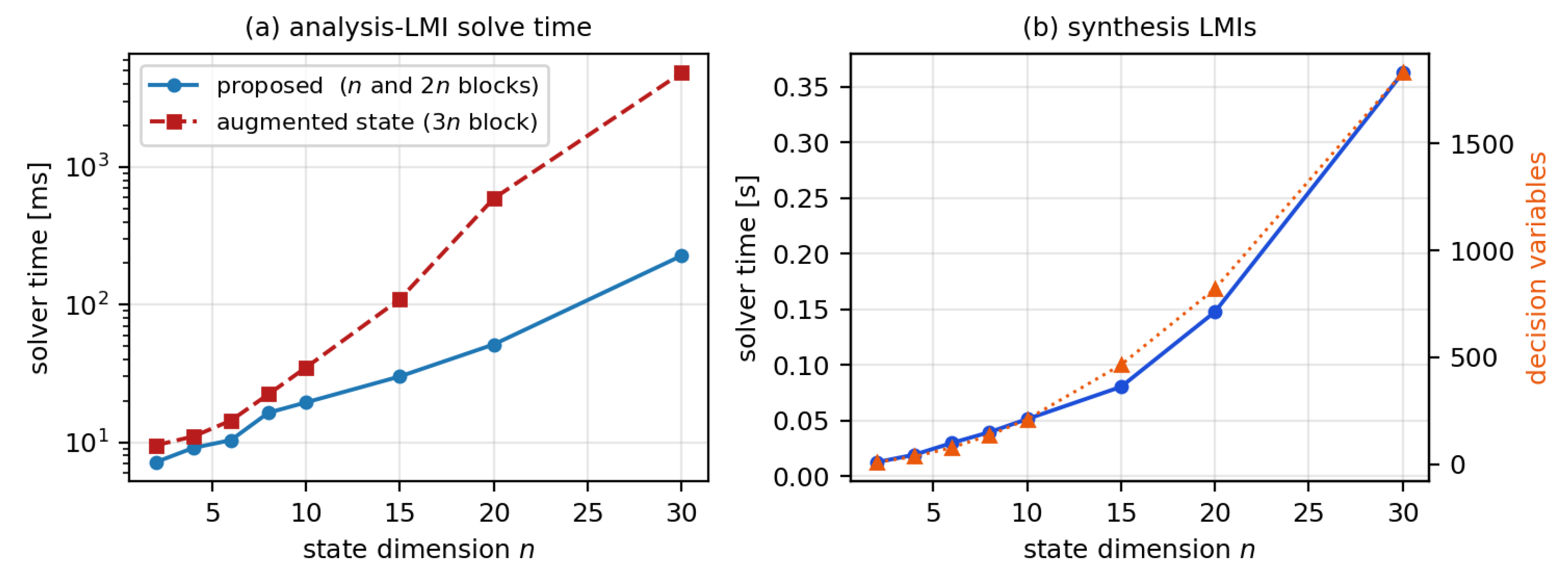
and two semidefinite blocks of sizes ( 2 n + m ) and 3 n —the largest matrix that the solver ever factorises has size max { 2 n + m , 3 n } , which is 3 n only because of the two auxiliary identity blocks introduced by the Schur completion of the weights; the genuine coupling blocks have sizes n and 2 n . An interior-point method requires O ( N var 2 i k i 2 + N var i k i 3 ) operations per iteration for blocks of sizes k i , so the cost of the proposed formulation grows as O ( n 6 ) in the worst case with a small constant. By contrast, an augmented-state formulation on col { e , e d , D a ς C H e } carries a single dense 3 n × 3 n block and 3 n 2 + n ( n + 1 ) / 2 variables. The ratio of variable counts tends to 3 for large n, and because the leading term is quadratic in the number of variables, the measured ratio of solver times grows much faster: Section 4.5 reports 1.33 at n = 2 and 21.33 at n = 30 . In absolute terms the synthesis LMIs are solved in 0.013  s at n = 2 and 0.363  s at n = 30 (Section 4.6), so dimensions of a few tens pose no difficulty on a standard laptop. For q delays, the variable count becomes n ( n + 1 ) ( q + 1 ) / 2 + n ( n + 1 ) / 2 + m n and q blocks of size 3 n are added, so the growth in q is linear.
Remark 13 
(Selection of α e , β e and of the weights S, S d , R). The conditions of Theorem 3 are LMIs only after α e and β e have been fixed, so their choice is part of the design. The following rules follow from the structure of the conditions and are confirmed by the grid search reported in Section 4.7.
 (i) 
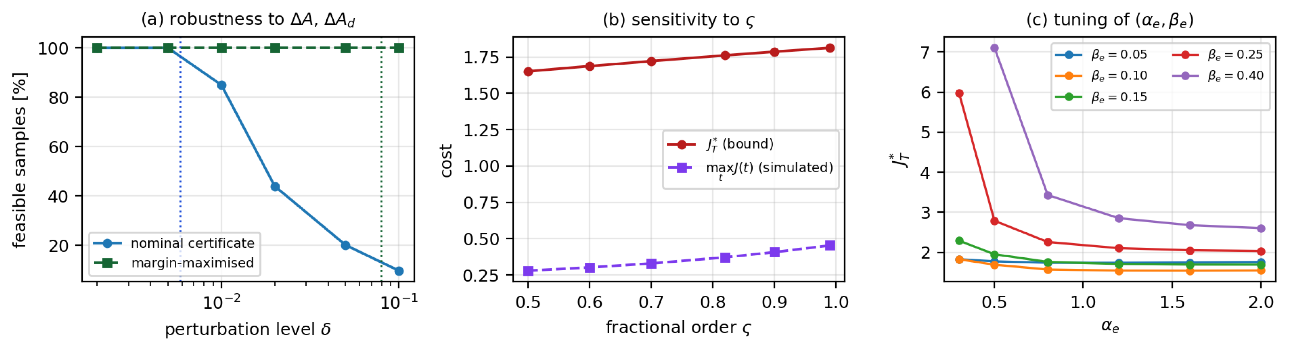
Role of β e . β e must be large enough for the delay-channel block to admit a solution: by Corollary 1, a necessary condition is β e P > 2 S d ; hence, β e > 2 λ max ( S d ) / λ min ( P ) . Increasing β e beyond that threshold relaxes Equation (57) but enters J T * linearly through β e V ¯ and also through V ¯ = V a / ( 1 β e / α e ) . The bound therefore degrades quickly for large β e : in the grid search of Section 4.7, at  α e = 0.80 , J T * rises from 1.5724 at β e = 0.10 to 3.4318 at β e = 0.40 .
 (ii) 
Role of α e . α e must satisfy α e > β e and enters Equation (55) through + α e W , so a large α e tightens the main inequality and forces a larger gain: K grows from 0.168 at α e = 0.80 to 0.554 at α e = 2.00 (with β e = 0.10 ). Conversely a large α e improves V ¯ . The resulting trade-off is flat near the optimum, which makes the tuning easy in practice.
 (iii) 
A concrete rule. Start from β e 2 λ max ( S d ) / λ min ( P 0 ) for a rough P 0 (for instance, P 0 = I ), take α e 10 β e , and then refine on a small logarithmic grid minimising J T * . On the benchmark, this rule gives ( α e , β e ) = ( 1.60 , 0.10 ) with J T * = 1.54359 , a reduction of 12.4 % with respect to the value J T * = 1.76146 obtained at the initial choice ( 0.80 , 0.15 ) .
 (iv) 
Weights. S, S d and R are performance specifications, not tuning knobs; they should be fixed by the application. Their influence on feasibility is monotone: increasing S or R tightens Equation (55), while increasing S d tightens Equation (57), and by Corollary 1, the delay block becomes infeasible as soon as 2 S d β e P . A larger R penalises control effort and yields a smaller K at the price of slower error decay.
 (v) 
Margin maximisation. If robustness rather than nominal cost is the priority, replace the feasibility problem by max ϵ subject to Equation (55) ϵ I , Equation (57) ϵ I and I W κ I . This is still an LMI. Section 4.7 shows that it enlarges the guaranteed perturbation radius from 0.005853 to 0.079517 , that is, by a factor of 13.6 .

3.4. Design Algorithm

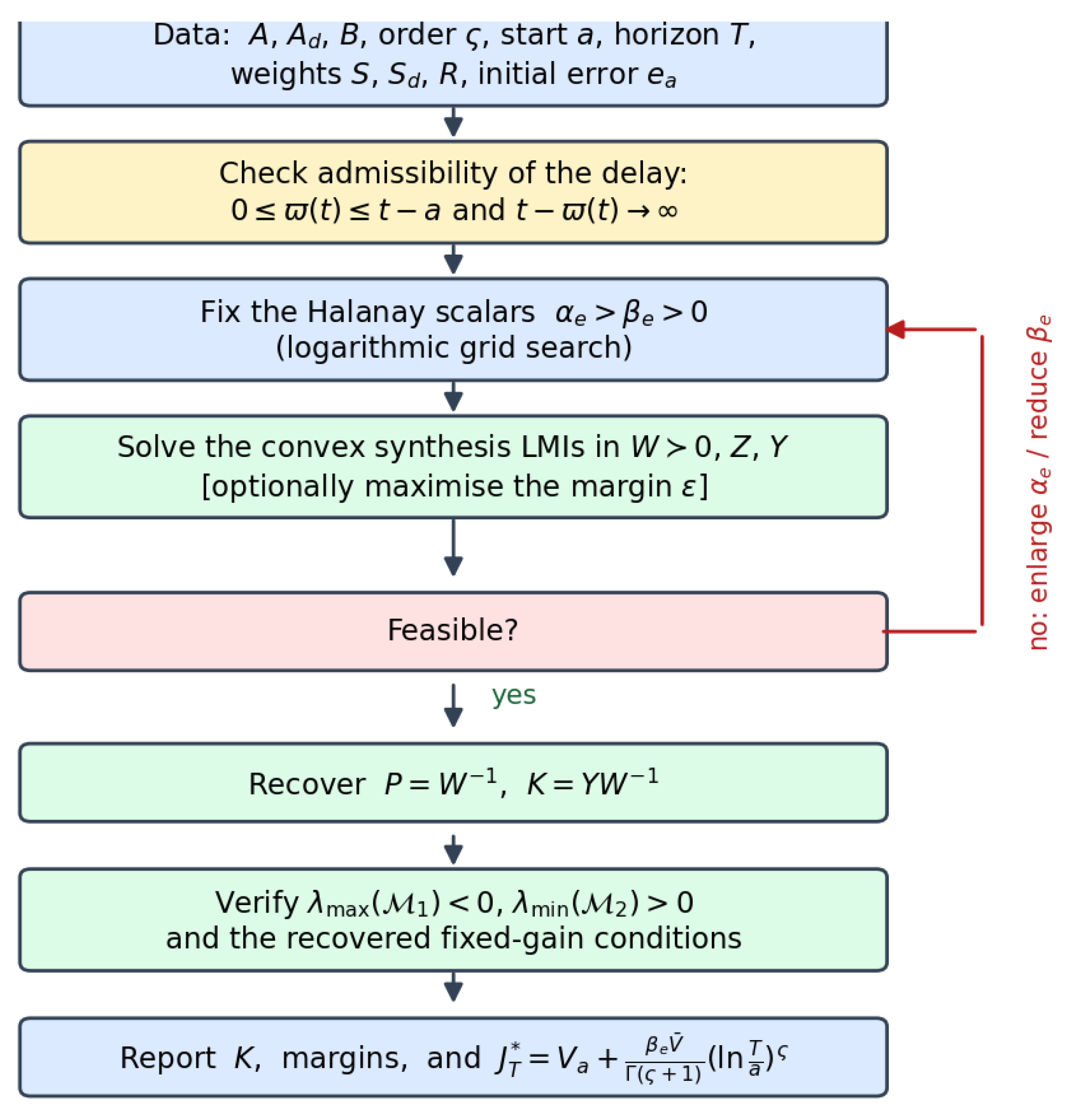
The complete design procedure is summarised in Algorithm 1 and displayed as a flowchart in Figure 1.
Algorithm 1 Convergence-to-zero guaranteed-cost synchronization design
Require: 
A, A d , 1 , , A d , q , B, order ς ( 0 , 1 ) , initial instant a > 0 , horizon T > a , weights S , S d i , R 0 , initial error e a , delays ϖ i
Ensure: 
gain K, certificate ( P , R e i ) , guaranteed cost J T *
1:
Admissibility. Verify 0 ϖ i ( t ) t a and t ϖ i ( t ) for every i (Assumption 1). If it fails, stop: the framework does not apply.
2:
Initialise the scalars. Choose β i > 0 with i β i < α e , following Remark 13(iii).
3:
Solve the convex program. Solve (55)–(57) (or (66) and (67) for q > 1 , or (72) and (73) under uncertainty) in W 0 , Z i = Z i T , Y. Optionally maximise the margin ϵ as in Remark 13(v).
4:
if infeasible then
5:
      increase α e , or increase β i towards 2 λ max ( S d i ) / λ min ( P ) , and return to step 3
6:
end if
7:
Recover. Set P W 1 , K Y W 1 , R e i P Z i P .
8:
Verify. Compute λ max ( M 1 ) < 0 and λ min ( M 2 i ) > 0 for the synthesis blocks, and  λ max , λ min of the recovered fixed-gain conditions (32)–(33), by direct eigenvalue evaluation.
9:
Certify the cost.  V a 1 2 e a T P e a , V ¯ V a / ( 1 i β i / α e ) , J T * V a + i β i V ¯ ln ( T / a ) ς / Γ ( ς + 1 ) .
10:
return K, ( P , R e i ) , J T * and all margins.

3.5. Extension to Several Admissible Delays

Assumption 1 and the whole argument of Theorem 2 are pointwise in the delayed variable, which makes the extension to q simultaneous delays immediate. Consider
D a ς C H e ( t ) = A K e ( t ) + i = 1 q A d , i e t ϖ i ( t ) , e ( a ) = e a ,
with A d , i R n × n and each ϖ i satisfying Assumption 1, and the cost density
( t ) = e T ( t ) S e ( t ) + i = 1 q e T t ϖ i ( t ) S d i e t ϖ i ( t ) + u T ( t ) R u ( t ) .
Theorem 4 
(Multiple-delay synthesis). Fix scalars α e > 0 and β 1 , , β q > 0 with
α e > i = 1 q β i .
Suppose that there exist W = W T > 0 , Z i = Z i T ( i = 1 , , q ) and Y R m × n such that
Φ W q 2 W S 1 / 2 2 Y T R 1 / 2 I 0 * I < 0 , Φ W q = A W + W A T B Y Y T B T + i = 1 q Z i + α e W ,
and, for every i = 1 , , q ,
Z i A d , i W 0 β i W 2 W S d i 1 / 2 I 0 .
Let P = W 1 and K = Y W 1 . Then, u ( t ) = K e ( t ) achieves convergence synchronization for Equation (63), and for every T > a , the cost in Equation (13) built on Equation (64) satisfies J ( t ) J T , q * for a t T , where
J T , q * = V a + i = 1 q β i V ¯ q Γ ( ς + 1 ) ln T a ς , V a = 1 2 e a T P e a , V ¯ q = V a 1 i = 1 q β i / α e .
Proof. 
As in Theorem 3, pre- and post-multiplying Equation (66) after a Schur complement by P, and Equation (67) by diag ( P , P ) , gives the fixed-gain conditions
sym ( P A K ) + i = 1 q R e i + α e P + 2 S + 2 K T R K < 0 , R e i P A d , i β i P 2 S d i 0 ,
with R e i = P Z i P . Put V e = 1 2 e T P e and e d , i ( t ) = e ( t ϖ i ( t ) ) . Lemma 1 and Equation (63) give
D a ς C H V e + 1 2 e T sym ( P A K ) + 2 S + 2 K T R K e + i = 1 q e T P A d , i e d , i + e d , i T S d i e d , i .
Each block inequality in Equation (69) yields, exactly as in Equation (45),
e T P A d , i e d , i + e d , i T S d i e d , i 1 2 e T R e i e + β i 2 e d , i T P e d , i = 1 2 e T R e i e + β i V e t ϖ i ( t ) .
Summing over i and using the first inequality of Equation (69) gives
D a ς C H V e + α e V e ( t ) + i = 1 q β i V e t ϖ i ( t ) α e V e ( t ) + i = 1 q β i sup ϖ max ( t ) η 0 V e ( t + η ) ,
where ϖ max ( t ) = max i ϖ i ( t ) again satisfies Assumption 1, being a maximum of finitely many admissible delays. Since 0 and α e > i β i by Equation (65), Lemma 2 applies with λ = α e and μ = i β i and gives V e ( t ) 0 ; hence, e ( t ) 0 . The cost bound follows verbatim from the argument of Theorem 2, with  β e replaced by i β i in Equation (49) and in Equation (51).    □
Remark 14. 
Condition (65) is the natural multi-channel version of α e > β e : the total delayed gain i β i must be dominated by the instantaneous decay rate α e . Each delay is handled by its own block in Equation (67), so the delays need not be of the same nature; Section 4.3 combines a bounded delay with an unbounded proportional one. The number of decision variables grows linearly in q and no augmentation of the state vector is required, in contrast with formulations that stack col { e , e d , 1 , , e d , q , D a ς C H e } and produce a block of size ( q + 2 ) n .

3.6. Extension to Norm-Bounded Parametric Uncertainty

In practice, A and A d are known only approximately. Consider the uncertain drive–response pair in which Equations (7) and (9) hold with A and A d replaced by
A ( t ) = A + M F ( t ) N a , A d ( t ) = A d + M F ( t ) N d , F T ( t ) F ( t ) I ,
where M R n × p , N a , N d R p × n are known, and F ( · ) is an unknown, possibly time-varying, Lebesgue-measurable matrix function. The error dynamics become
D a ς C H e ( t ) = A ( t ) B K e ( t ) + A d ( t ) e t ϖ ( t ) .
Theorem 5 
(Robust synthesis). Fix scalars α e > β e > 0 and ε 1 > 0 , ε 2 > 0 . Suppose that there exist W = W T > 0 , Z = Z T and Y R m × n such that
Φ W rob 2 W S 1 / 2 2 Y T R 1 / 2 W N a T I 0 0 I 0 ε 1 1 I < 0 , Φ W rob = Φ W + ε 1 1 + ε 2 1 M M T ,
with Φ W as in Equation (56), and
Z A d W 0 0 β e W 2 W S d 1 / 2 ε 2 W N d T I 0 I 0 .
Let P = W 1 , K = Y W 1 and
R e = P Z P + ε 2 1 P M M T P .
Then, u ( t ) = K e ( t ) achieves convergence synchronization for Equation (71) and the finite-horizon cost bound in Equation (37) holds, for  every admissible uncertainty F ( · ) with F T F I and every delay satisfying Assumption 1.
Proof. 
A Schur complement on the last block of Equation (72), followed by the Schur complements on the two I blocks and by pre- and post-multiplication by P, converts Equation (72) into
sym ( P A K ) + P Z P + ε 1 1 P M M T P + ε 2 1 P M M T P + ε 1 N a T N a + α e P + 2 S + 2 K T R K < 0 .
Similarly, Schur complements on the last two blocks of Equation (73) and pre- and post-multiplication by diag ( P , P ) give
P Z P P A d β e P 2 S d ε 2 N d T N d 0 .
Let V e = 1 2 e T P e . Since sym P ( A ( t ) B K ) = sym ( P A K ) + sym P M F N a , Lemma 1 applied to Equation (71) gives
D a ς C H V e + 1 2 e T sym ( P A K ) + sym P M F N a + 2 S + 2 K T R K e + e T P A d ( t ) e d + e d T S d e d .
For any ε > 0 and any F with F T F I , one has the elementary bound 2 ξ T P M F N ζ ε 1 ξ T P M M T P ξ + ε ζ T N T N ζ . Applying it with ε = ε 1 , N = N a , ζ = e gives
e T sym P M F N a e ε 1 1 e T P M M T P e + ε 1 e T N a T N a e ,
and with ε = ε 2 , N = N d , ζ = e d , it gives
2 e T P M F N d e d ε 2 1 e T P M M T P e + ε 2 e d T N d T N d e d .
Inequality (76) states, for all ξ , ζ R n , that
2 ξ T P A d ζ + 2 ζ T S d ζ + ε 2 ζ T N d T N d ζ ξ T ( P Z P ) ξ + β e ζ T P ζ .
Adding the last two displays with ξ = e , ζ = e d and dividing by two yields
e T P A d ( t ) e d + e d T S d e d 1 2 e T R e e + β e V e t ϖ ( t ) ,
with R e as in Equation (74). Substituting this and the ε 1 bound into the expression for D a ς C H V e + , and then invoking Equation (75), gives
D a ς C H V e + α e V e ( t ) + β e V e t ϖ ( t ) ,
which is exactly Equation (47). The remainder of the proof of Theorem 2 applies verbatim and is independent of F.    □
Remark 15. 
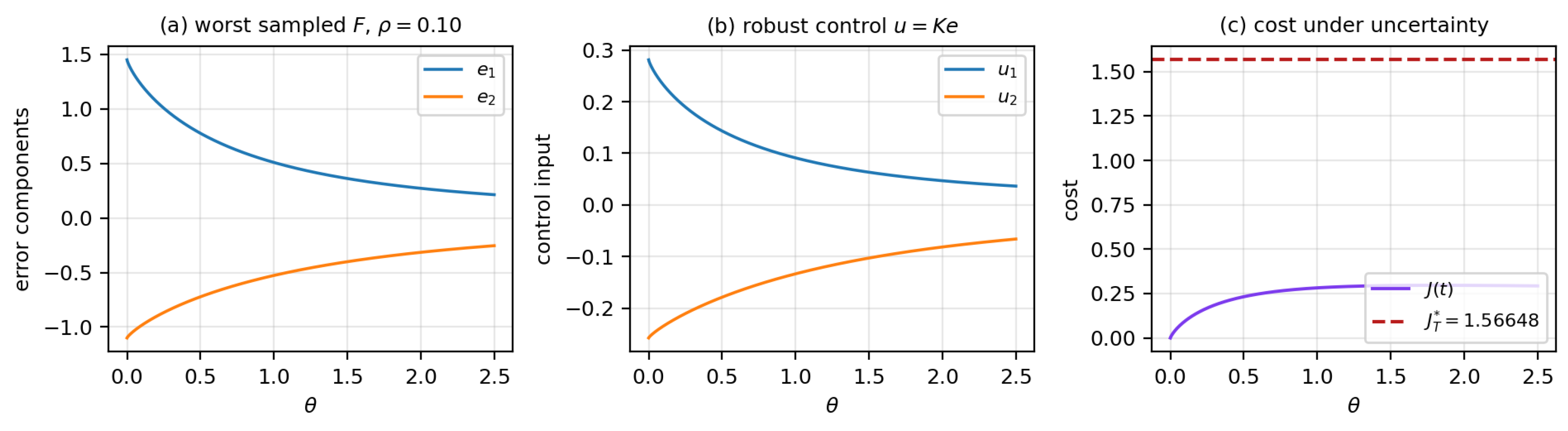
Three points are worth noting. (i) The scalars ε 1 , ε 2 play the same role as α e , β e : they must be fixed before solving, after which Equations (72) and (73) are LMIs, and a coarse logarithmic line search over them is sufficient in practice (Section 4.4). (ii) The recovered delay-channel matrix is Equation (74) and not P Z P ; the additional term ε 2 1 P M M T P is precisely the price paid for the uncertainty entering the delayed channel, and omitting it invalidates the verification. (iii) Taking M = 0 recovers Theorem 3 exactly. The structure Equation (70) covers, in particular, independent norm-bounded perturbations Δ A ρ , Δ A d ρ by choosing M = ρ I , N a = N d = I ; this is the form used in Section 4.4. Exogenous disturbances, which would call for an input-to-state or H formulation rather than a guaranteed-cost one, are not covered and are listed in Section 5.
Proposition 3. 
If the hypotheses of Theorem 1 and Theorem 3 hold for the same admissible delay, then
lim t x ( t ) = 0 , lim t e ( t ) = 0 , lim t y ( t ) = 0 .
Proof. 
The first two limits follow directly from Theorems 1 and 3. Since e ( t ) = x ( t ) y ( t ) , one has y ( t ) = x ( t ) e ( t ) . Therefore, x ( t ) 0 and e ( t ) 0 imply y ( t ) 0 .    □

4. Numerical Examples

This section gives a certificate-based numerical validation of the single-delay convergence theory and the guaranteed-cost synthesis theorem. The purpose is two-fold: to verify the hypotheses of the theorems through strict matrix margins, and to illustrate the finite-horizon behaviour of the closed-loop trajectories. The asymptotic convergence conclusion is not inferred from the finite-time plots; it follows from the verified LMI certificates and the Caputo–Hadamard Halanay inequality. The controller-synthesis LMI is solved in Python 3.12.10 using CVXPY 1.9.1 and then independently checked by direct eigenvalue evaluation. The section is organised as follows. Section 4.1 is the baseline single-delay design. Section 4.2 treats an unbounded admissible delay with the same certificate. Section 4.3 is a four-dimensional, two-delay, under-actuated design. Section 4.4 treats norm-bounded parametric uncertainty. Section 4.5 compares the proposed conditions with augmented-state and norm-bound formulations, Section 4.6 reports a scalability study up to n = 30 , and Section 4.7 presents a sensitivity study. All solver settings, versions and timings are collected in Table 3, so that every number below is reproducible.

4.1. Example 1: Baseline Single-Delay Design

Let n = 2 , m = 2 , a = 1 , ς = 0.82 , and 
A = 1.00 0.25 0.15 0.90 , A d = 0.080 0.030 0.020 0.050 , B = I 2 .
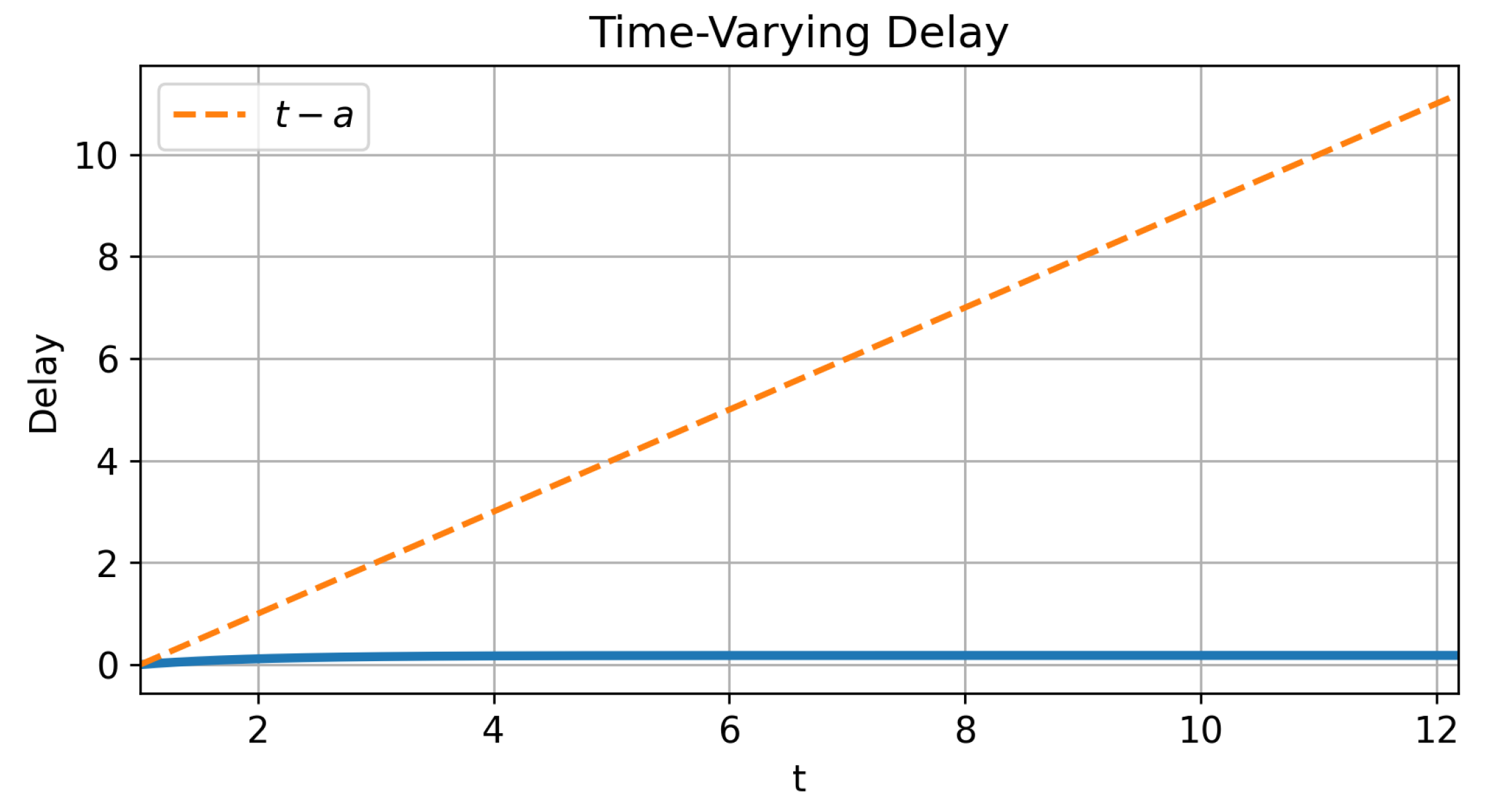
The single time-varying delay is
ϖ ( t ) = 0.18 1 e ( t 1 ) , t 1 .
Clearly 0 ϖ ( t ) 0.18 . Furthermore, since 1 e r r for r 0 ,
ϖ ( t ) 0.18 ( t 1 ) < t 1 , t > 1 ,
and hence t ϖ ( t ) 1 and t ϖ ( t ) . Thus, Assumption 1 is satisfied. Notice that the condition t ϖ ( t ) also permits some unbounded delays, provided the delayed argument still tends to infinity; the present example uses a bounded admissible delay, and Section 4.2 treats an unbounded one.
For Theorem 1, a feasible certificate is obtained with
P x = I 2 , α x = 0.60 , β x = 0.08 ,
and
R x = 0.10125000 0.00125000 0.00125000 0.04625000 .
Then,
M x = sym ( P x A ) + R x + α x P x
has eigenvalues
λ ( M x ) = { 1.35078037 , 1.10171963 } .
Thus, Equation (17) is strictly satisfied. The delay-channel matrix
L x = R x P x A d 0.08 P x
has eigenvalues
λ ( L x ) = { 0.00452611 , 0.00669296 , 0.11952865 , 0.17675229 } .
Therefore, Equation (18) is strictly feasible. Finally,
α x β x = 0.52000000 > 0 ,
so the scalar Halanay condition is satisfied. Theorem 1 gives x ( t ) 0 .
For the cost weights, take
S = 0.20 I 2 , S d = 0.010 I 2 , R = 0.050 I 2 .
The synthesis scalars are fixed before solving the LMI problem:
α e = 0.80 , β e = 0.15 .
The CVXPY feasibility problem uses W = W T , Z = Z T , and Y as decision variables, with the normalization W I 2 . The reported certificate corresponds to a CVXPY/SCS solution for which the solver status is optimal, and all matrix inequalities are subsequently verified by direct eigenvalue computation. The synthesis problem has 10 scalar decision variables and semidefinite blocks of sizes 6 and 6, and is solved in 0.013  s under the settings of Table 3. The returned matrices are
W = 1.33096481 0.00475288 0.00475288 1.32419792 , Z = 0.10972233 0.00184544 0.00184544 0.04036764 ,
Y = 0.22329597 0.06519651 0.06490558 0.12726490 .
Therefore,
P = W 1 = 0.75134429 0.00269676 0.00269676 0.75518380 ,
and the recovered controller gain is
K = Y W 1 = 0.16759633 0.04863317 0.04842323 0.09593336 .
With
Φ W = A W + W A T B Y Y T B T + Z + α e W ,
the main CVXPY synthesis LMI
M 1 = Φ W 2 W S 1 / 2 2 Y T R 1 / 2 I 0 I
has eigenvalues
λ ( M 1 ) = { 1.87096505 , 1.84868042 , 0.17639703 , 0.17505206 , 1.00000000 , 1.00000000 } .
Thus, λ max ( M 1 ) = 0.17505206 < 0 . The delay-channel synthesis matrix
M 2 = Z A d W 0 β e W 2 W S d 1 / 2 I
has eigenvalues
λ ( M 2 ) = { 0.01967233 , 0.00771722 , 0.24720270 , 0.18919886 , 1.04289161 , 1.04168166 } .
Thus, λ min ( M 2 ) = 0.00771722 > 0 . Moreover,
α e β e = 0.65000000 > 0 .
All synthesis hypotheses of Theorem 3 are therefore satisfied.
For a direct check of Theorem 2, set R e = P Z P . Then,
R e = 0.06194803 0.00135165 0.00135165 0.02303008 .
The recovered fixed-gain inequalities have eigenvalue margins
λ sym ( P ( A B K ) ) + R e + α e P + 2 S + 2 K T R K = { 0.18627484 , 0.18458822 } ,
and
λ R e P A d β e P 2 S d = { 0.14325900 , 0.11201961 , 0.01125066 , 0.00442806 } .
These values independently confirm that the CVXPY solution satisfies the gain-dependent conditions recovered by the Schur-complement proof.
Corollary 1 can also be checked on these data. Here, β e P 2 S d has eigenvalues { 0.09249306 , 0.09348615 } , so it is positive definite and
R e min = P A d β e P 2 S d 1 A d T P = 0.04455238 0.00080161 0.00080161 0.01769761 ,
with λ R e R e min = { 0.00530745 , 0.01742067 } 0 , exactly as predicted by Equation (52). Replacing R e by R e min improves the main margin from 0.18458822 to 0.19022203 , which quantifies how little is lost by the affine parametrisation actually used by the solver.
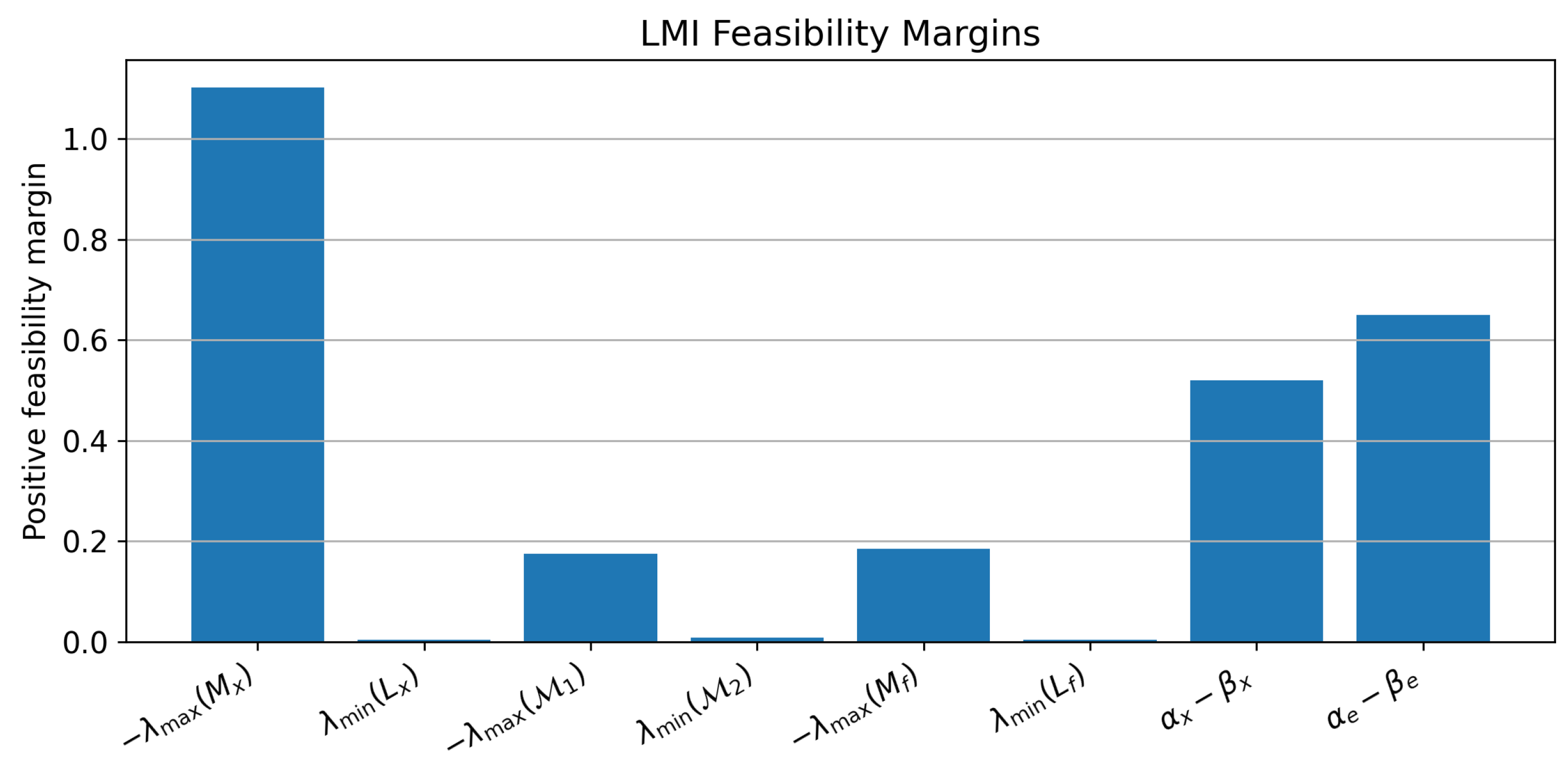
All the verified eigenvalue margins of this example are displayed in Figure 2 and collected in Table 4.
The simulation is carried out with step size 2.5 / 1200 in logarithmic time θ = ln ( t / a ) . Thus, the final physical time is T = e 2.5 12.1825 . Under this transformation, the Caputo–Hadamard derivative becomes a Caputo derivative in θ , while the delayed logarithmic argument is
θ d ( θ ) = ln a e θ ϖ ( a e θ ) a .
It is not approximated by θ ϖ ( θ ) . A fractional Adams-type integral discretization is used for the transformed Caputo delay system [41]; delayed values are obtained by interpolation on the computed logarithmic-time grid.
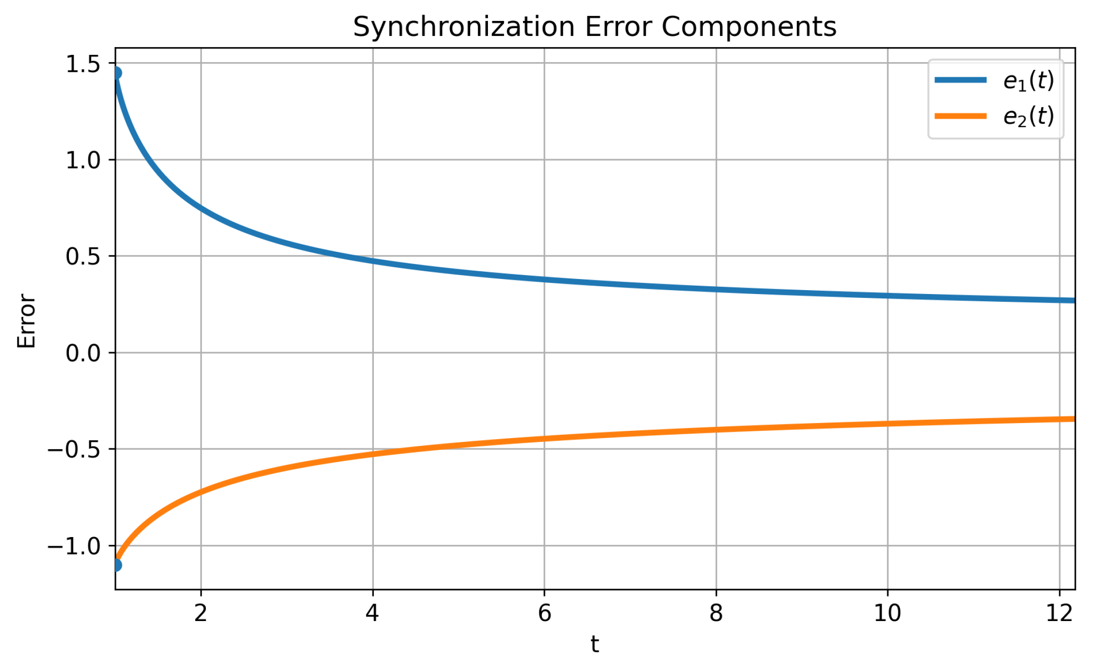
The initial values are
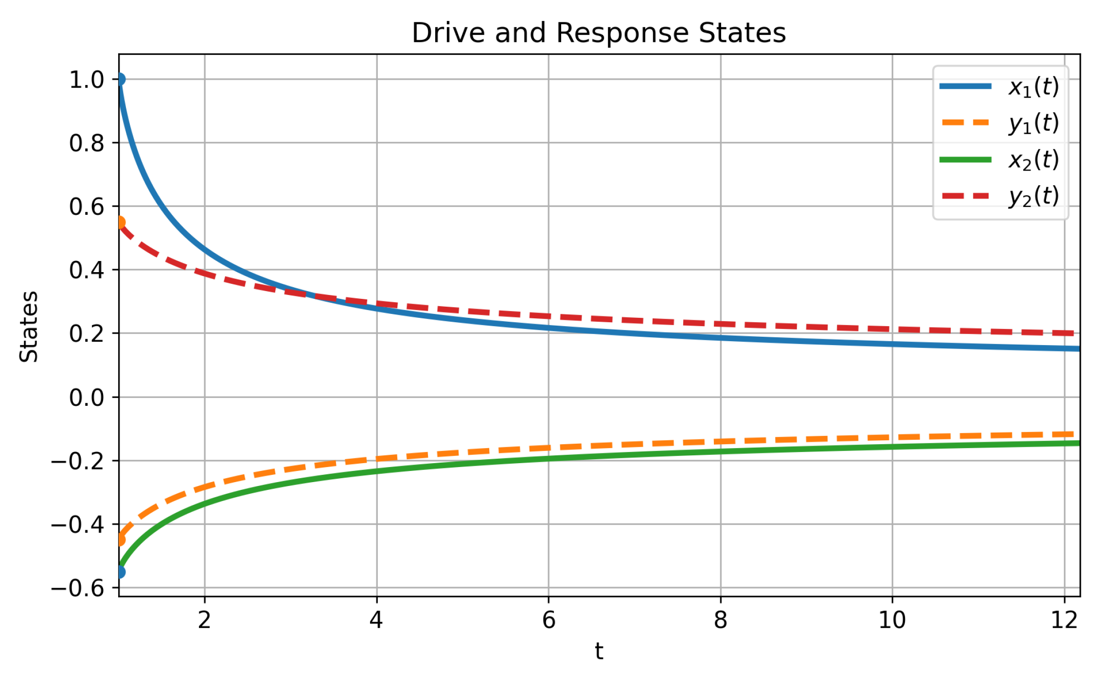
x a = 1.00 0.55 , e a = 1.45 1.10 , y a = x a e a = 0.45 0.55 .
The first simulated points are
x [ 0 ] = 1.00000000 0.55000000 , x [ 1 ] = 0.99296660 0.54771972 , e [ 0 ] = 1.45000000 1.10000000 , e [ 1 ] = 1.44135528 1.09614373 , y [ 0 ] = 0.45000000 0.55000000 , y [ 1 ] = 0.44838868 0.54842401 .
These nonzero initial values confirm that the simulation is not a trivial zero-trajectory validation.
Using Equation (88), the initial Lyapunov value is
V a = 1 2 e a T P e a = 1.24243555 .
With β e / α e = 0.1875 ,
V ¯ = V a 1 β e / α e = 1.52915145 .
For the simulation horizon θ T = ln ( T / a ) = 2.5 , Theorem 3 gives
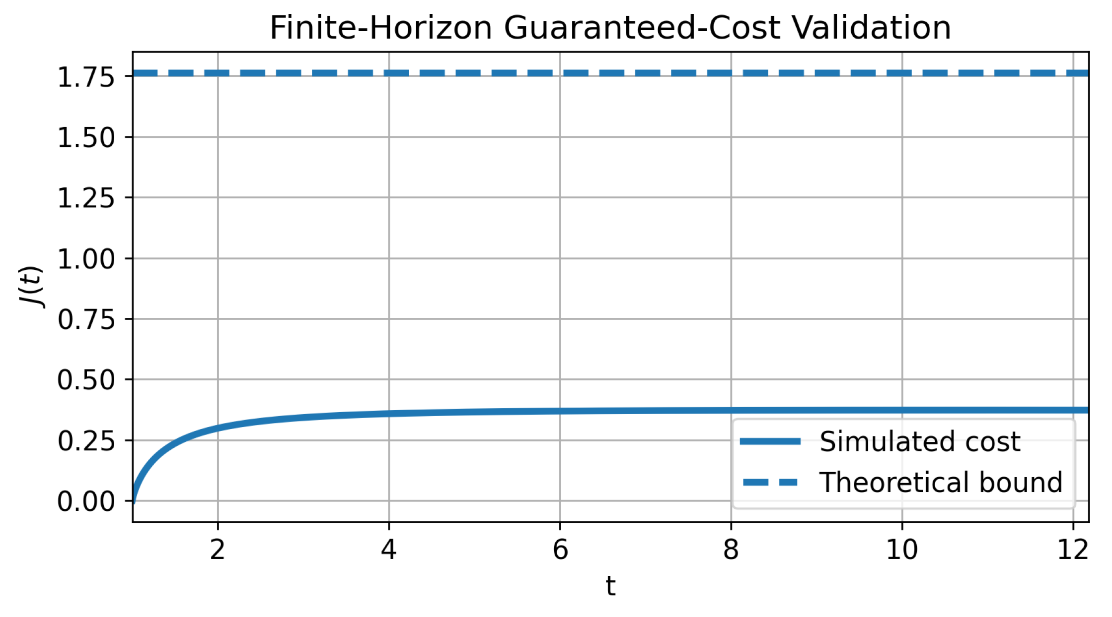
J T * = V a + β e V ¯ Γ ( ς + 1 ) θ T ς = 1.76145638 .
The simulated maximum cost is
max 0 θ 2.5 J ( t ) = 0.37226435 < J T * .
The finite-horizon bound is conservative, as expected, but it is an a priori guaranteed upper bound computed only from the initial error, horizon, and feasible LMI variables.
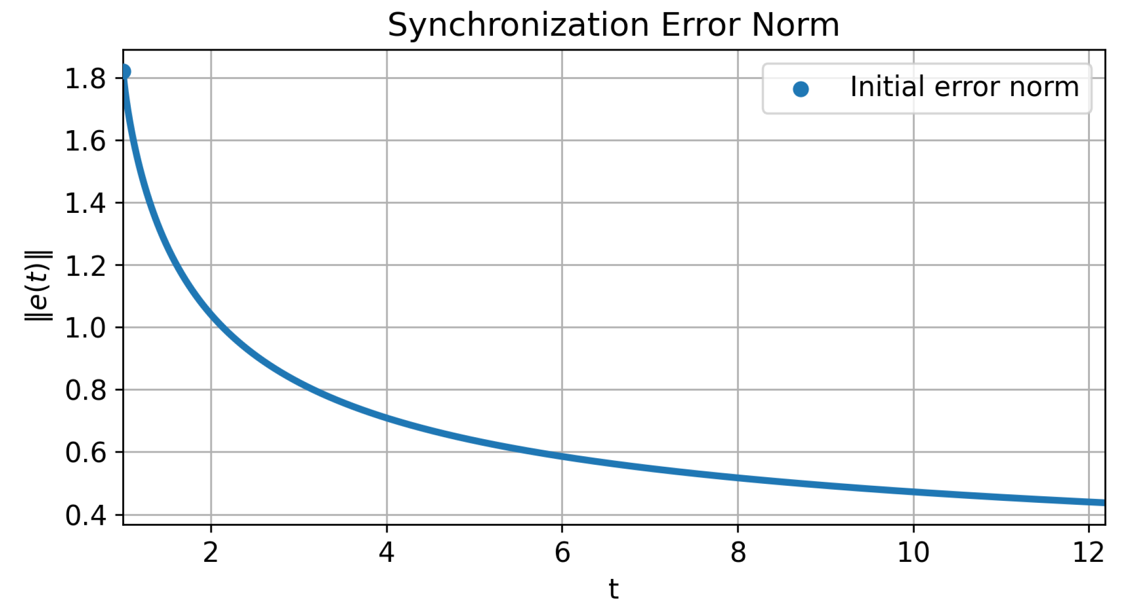
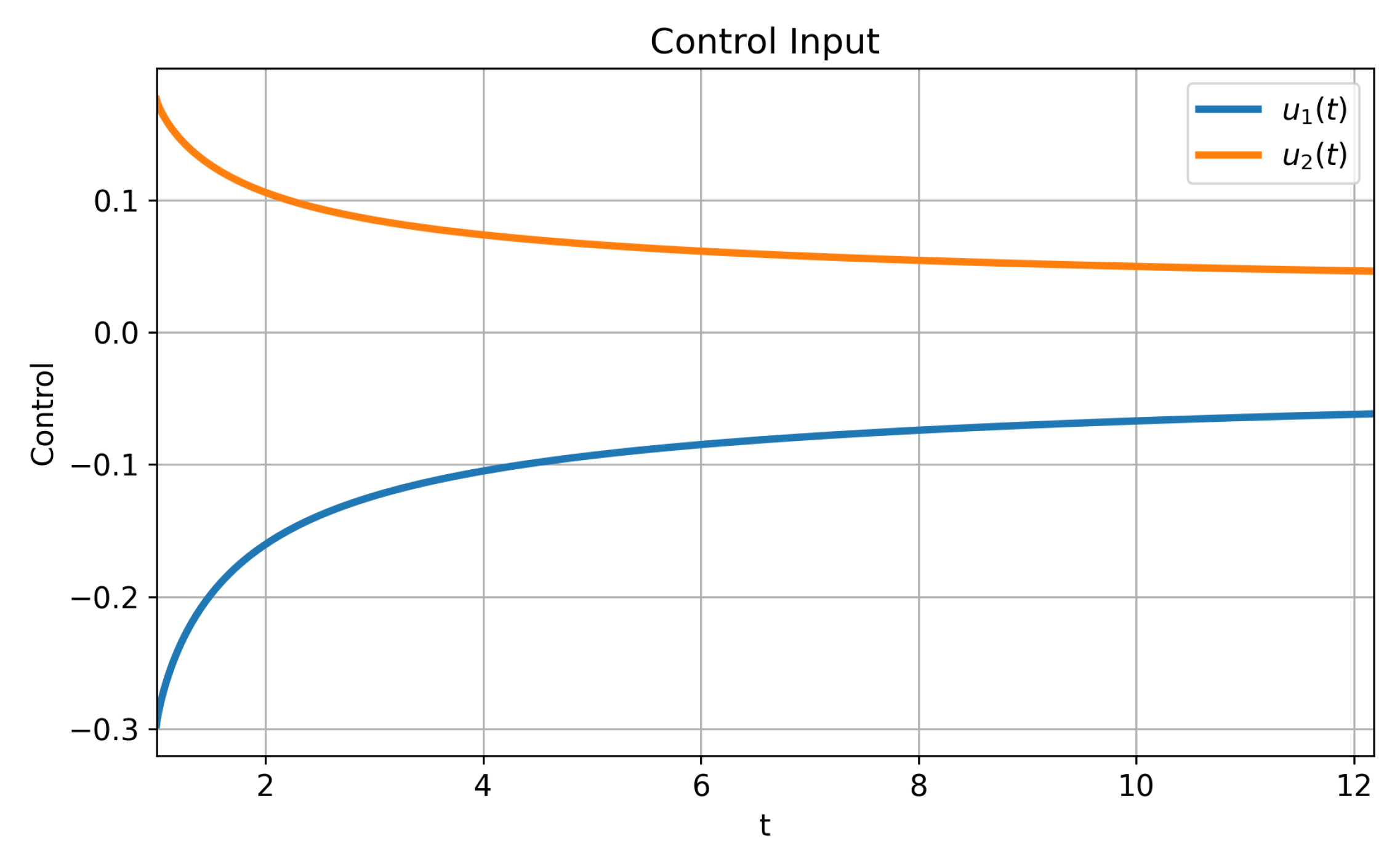
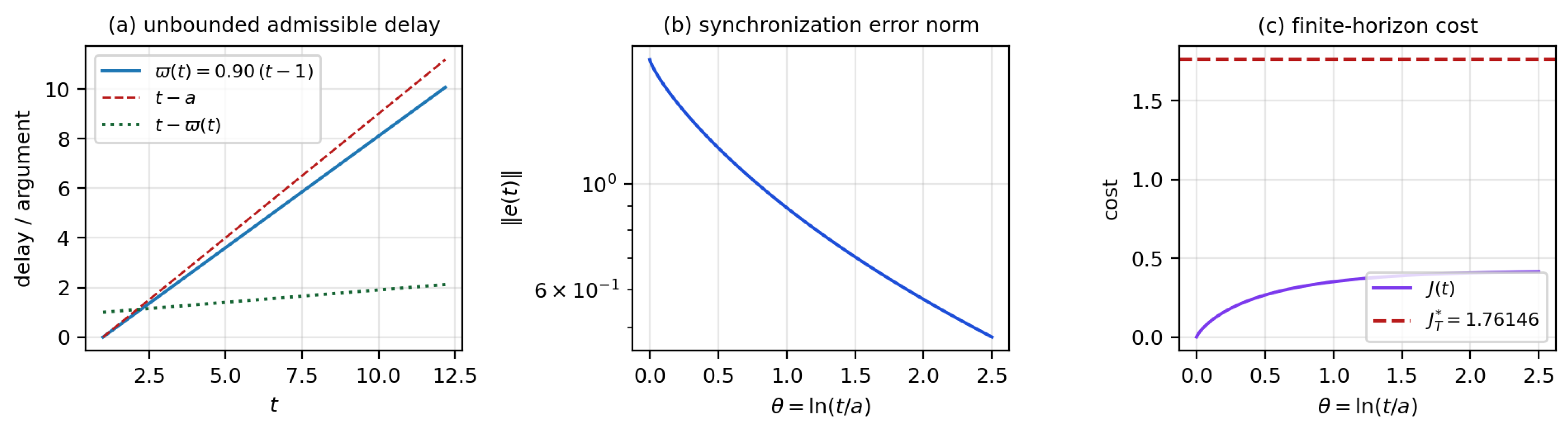
The simulation results are reported in Figure 3, Figure 4, Figure 5, Figure 6, Figure 7 and Figure 8: Figure 3 displays the delay in Equation (78) together with the admissibility bound t a , Figure 4 the drive and response state trajectories, Figure 5 the synchronization-error components, Figure 6 the error norm, Figure 7 the control input u ( t ) = K e ( t ) , and Figure 8 the simulated cost against the a priori bound in Equation (101).

4.2. Example 2: An Unbounded Admissible Delay

Assumption 1 allows delays that are not bounded, and this example exhibits one of them. Keep the data from Equation (77), the weights from Equation (84), the scalars from Equation (85), the certificate from Equations (86)–(89) and the initial conditions from Equation (98), and replace the delay from Equation (78) by the proportional (pantograph-type) delay
ϖ ( t ) = 0.90 ( t 1 ) , t 1 .
Admissibility is immediate: 0 ϖ ( t ) t 1 = t a and t ϖ ( t ) = 0.1 t + 0.9 . The delay is nevertheless unbounded, and at the end of the simulation horizon T = e 2.5 = 12.182494 , it reaches ϖ ( T ) = 10.064245 ; that is, it consumes 90 % of the whole elapsed history, while the delayed argument is still only t ϖ ( t ) = 2.118249 . This is far outside the reach of any bounded-delay criterion.
Because neither Equation (32) nor Equation (33) involves ϖ , no new synthesis is required: the certificate of Section 4.1 remains valid verbatim, and so does the bound J T * = 1.76145638 . The simulation confirms this. Starting from e ( a ) = 1.82002747 , the error decreases monotonically to e ( T ) = 0.47803811 , and the simulated cost attains
max 0 θ 2.5 J ( t ) = 0.41503079 < J T * = 1.76145638 .
Comparison with Equation (102) shows that increasing the delay from a bound of 0.18 to an unbounded profile raises the simulated cost by only 11.5 % and leaves the a priori bound unchanged, which is the practical meaning of the delay-rate independence discussed in Remark 2(d). Figure 9 displays the delay together with the constraint t a , the error norm and the cost.

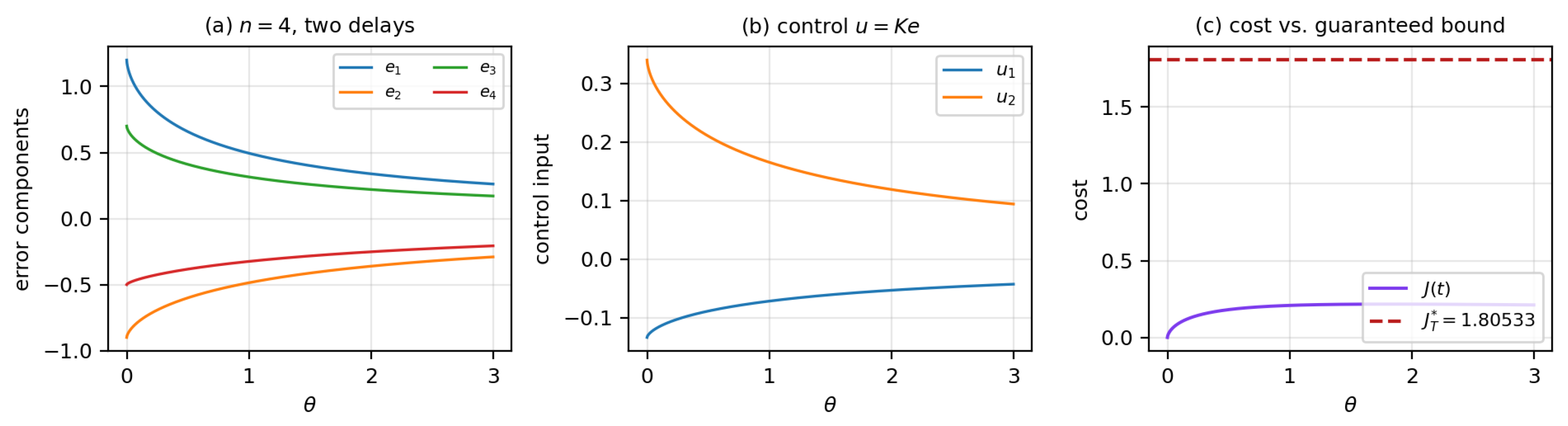
4.3. Example 3: A Four-Dimensional Under-Actuated System with Two Delays

This example tests Theorem 4 on a system that is larger than the benchmark, has fewer inputs than states, uses a different fractional order and carries two delays of different natures. Take n = 4 , m = 2 , a = 1 , ς = 0.65 and
A = 0.90 0.30 0.00 0.10 0.20 1.10 0.25 0.00 0.10 0.00 0.95 0.20 0.00 0.15 0.10 1.05 , B = 1.00 0.00 0.00 1.00 0.50 0.20 0.20 0.50 ,
A d , 1 = 0.06 0.02 0.01 0.00 0.01 0.05 0.00 0.02 0.00 0.01 0.07 0.01 0.02 0.00 0.01 0.04 , A d , 2 = 0.03 0.01 0.00 0.01 0.00 0.02 0.01 0.00 0.01 0.00 0.03 0.01 0.01 0.01 0.00 0.02 ,
with the two delays
ϖ 1 ( t ) = 0.25 1 e ( t 1 ) ( bounded ) , ϖ 2 ( t ) = 0.60 ( t 1 ) ( unbounded ) ,
which are both admissible. The weights are S = 0.15 I 4 , S d 1 = 0.008 I 4 , S d 2 = 0.005 I 4 , R = 0.040 I 2 , and the Halanay scalars are α e = 0.90 , β 1 = 0.10 , β 2 = 0.08 , so that the condition in Equation (65) holds with the margin α e ( β 1 + β 2 ) = 0.72000000 > 0 .
The synthesis problem in Equations (66) and (67) has 38 scalar decision variables and is solved in 0.0373  s, with solver status optimal. It returns
W = 1.32650678 0.03809049 0.14133819 0.03053944 0.03809049 1.33276175 0.03011217 0.14694998 0.14133819 0.03011217 1.49152876 0.02965466 0.03053944 0.14694998 0.02965466 1.52153306 ,
Z 1 = 0.16254018 0.03818870 0.05786350 0.02054473 0.03818870 0.15354636 0.02068584 0.10058715 0.05786350 0.02068584 0.26653075 0.00843073 0.02054473 0.10058715 0.00843073 0.30832792 , Z 2 = 0.08147980 0.04267260 0.08797917 0.03323054 0.04267260 0.08873678 0.02867150 0.11751124 0.08797917 0.02867150 0.22225506 0.02240066 0.03323054 0.11751124 0.02240066 0.26527893 ,
Y = 0.00192149 0.16648116 0.02312995 0.00247409 0.02242945 0.25781664 0.26405965 0.03560486 ,
from which
P = W 1 = 0.76242459 0.01851433 0.07217071 0.01492149 0.01851433 0.75926709 0.01503065 0.07325151 0.07217071 0.01503065 0.67791579 0.01611281 0.01492149 0.07325151 0.01611281 0.66492004 ,
K = Y W 1 = 0.00324968 0.12620167 0.01299930 0.01349605 0.04146272 0.18958986 0.17732750 0.00937835 .
All hypotheses of Theorem 4 are verified by direct eigenvalue evaluation; the margins are collected in Table 5. Note that the two delay channels do not carry the same margin: the second, which corresponds to the unbounded delay and the smaller weight β 2 , is about five times tighter than the first, which is the expected behaviour since β i controls the size of the i-th block through Equation (67).
With x a = [ 0.80 , 0.60 , 0.45 , 0.30 ] T and e a = [ 1.20 , 0.90 , 0.70 , 0.50 ] T , so that e a = 1.72916165 , and a horizon θ T = 3.0 , i.e.,  T = e 3 = 20.085537 , Formula (68) gives
V a = 1.19517363 , V ¯ q = 1.49396703 , J T , q * = 1.80533324 ,
while the simulated cost attains max t J ( t ) = 0.21681347 , and the error decreases to e ( T ) = 0.47381374 ; over this horizon, ϖ 2 grows to 11.451 . Figure 10 shows the error components, the two control channels and the cost. The example confirms that the framework operates without modification when m < n , when several delays of different natures act simultaneously, and at a different fractional order.

4.4. Example 4: Norm-Bounded Parametric Uncertainty

Theorem 5 is now applied to the benchmark of Section 4.1 perturbed by the uncertainty structure in Equation (70) with
M = ρ I 2 , N a = N d = I 2 , ρ = 0.10 ,
that is, arbitrary time-varying perturbations with Δ A ( t ) 0.10 and Δ A d ( t ) 0.10 . Since A = 1.041535 and A d = 0.085453 , this amounts to 9.6 % of the norm of A and to 117 % of the norm of A d : the delay matrix may be perturbed by more than its own size, and even its sign structure may be altered. With the scalars α e = 0.80 , β e = 0.15 retained and ε 1 = ε 2 = 0.02 chosen by a coarse logarithmic line search, the robust synthesis in Equations (72) and (73) is solved in 0.0281  s with status optimal and returns
W = 1.49800459 0.00184863 0.00184863 1.49583989 , Z = 0.16328030 0.00315913 0.00315913 0.06008477 , Y = 0.35175480 0.08062374 0.08036164 0.45689109 ,
hence
P = 0.66755571 0.00082500 0.00082500 0.66852177 , K = 0.23488244 0.05418892 0.05402280 0.30550794 ,
and, by Equation (74),
R e = P Z P + ε 2 1 P M M T P = 0.29558188 0.00208404 0.00208404 0.25031778 .
The recovered fixed-gain conditions are verified over the uncertainty set. At the nominal point F = 0 , they give λ max = 0.41261168 for the main condition and λ min = + 0.06590482 for the delay condition. Over 20,000 random matrices F with F 1 , the worst values observed are
max F λ max main = 0.28063157 < 0 , min F λ min delay = + 0.02407298 > 0 ,
with zero violations; the four probes F = ± I , F = diag ( 1 , 1 ) and F equal to the rotation by π / 4 give values in the same ranges. With  e a as in Equation (98), the guaranteed cost is V a = 1.10490774 , V ¯ = 1.35988645 and
J T * = 1.56647706 ,
which is 11.1 %  smaller than the nominal bound in Equation (101), because the robust design returns a better-conditioned P. Over 200 random realisations of F, the largest simulated cost is 0.29659321 , and the corresponding terminal error is e ( T ) = 0.33194929 ; the worst realisation is displayed in Figure 11.
Repeating the design for increasing ρ locates the practical limit of the method on these data. Table 6 shows that a certificate is obtained up to ρ = 0.75 , that is, for perturbations reaching 72 % of A , while the search grid returns no feasible point at ρ = 1.00 . The guaranteed cost degrades slowly, from  1.54654 at ρ = 0.05 to 2.30723 at ρ = 0.75 , whereas the required gain grows from K = 0.0764 to K = 5.3730 : robustness is bought with control authority, not with performance.

4.5. Comparison with Augmented-State and Norm-Bound Formulations

This subsection quantifies what the proposed delay-channel formulation costs in conservatism and what it saves in computation, relative to the alternatives. All comparisons use the data of Section 4.1 at the analysis level, that is, with the gain in Equation (89) held fixed and α e = 0.80 , β e = 0.15 , so that the four methods certify the same scalar Halanay inequality in Equation (47) and are therefore directly comparable. The methods are:
(M1)
The naive full-space augmented residual LMI Ψ < 0 of Equation (29) on col { e , e d , D a ς C H e } ;
(M2)
An augmented-state descriptor formulation, in which the residual A K e + A d e d D a ς C H e = 0 is adjoined with free weighting matrices N 1 , N 2 , N 3 R n × n , giving the 3 n × 3 n condition
sym ( N 1 T A K ) + S + K T R K + α e 2 P N 1 T A d + A K T N 2 1 2 P N 1 T + A K T N 3 sym ( N 2 T A d ) + S d β e 2 P N 2 T + A d T N 3 N 3 N 3 T < 0 ;
(M3)
The proposed pair of Equations (32) and (33) in ( P , R e ) ;
(M4)
The reduced single condition in Equation (54) of Corollary 1 in P alone;
(M5)
A classical delay-independent norm-bound Halanay criterion with P = I , requiring 1 2 λ max ( sym A K ) + A d + λ max ( S + K T R K + S d ) + α e β e 2 < 0 .
Conservatism is measured by the largest scaling ρ such that the method remains feasible when A d is replaced by ρ A d ; ρ is computed by bisection to a tolerance of 10 3 . The results are collected in Table 7.
Three conclusions follow.
(a)
(M1) fails structurally, as predicted. On these data, λ ( Ψ ) = { 0.20278700 , 0.20026923 , 0.04674302 , 0.04624651 , + 0.70209496 , + 0.70567214 } , so λ max ( Ψ ) = + 0.70567214 > 0 and the condition is infeasible for every ρ 0 , in exact agreement with Proposition 2. This is the obstruction that motivates the whole approach.
(b)
The proposed conditions are only marginally more conservative than (M2). The loss of admissible delay-channel gain is 1 4.4991 / 4.7005 = 4.29 % for (M3) and 1 4.5082 / 4.7005 = 4.09 % for (M4). In exchange, (M3) uses 60 % fewer decision variables than (M2), and (M4) uses 80 % fewer, and the largest block shrinks from 3 n to 2 n . The classical norm-bound criterion (M5) is free but loses 33.5 % of admissible gain, so it is not a competitive alternative.
(c)
The computational advantage grows with the dimension. At n = 2 , the two formulations are of comparable cost. Table 8 repeats the measurement for n up to 30: the ratio of solver times rises from 1.33 to 21.33 , and the ratio of decision variables tends to 3. The reason is that the leading term of the interior-point cost is quadratic in the number of variables and cubic in the block size, and (M2) is penalised on both counts.

4.6. Scalability of the Synthesis

The comparison above concerns the analysis step. Table 9 reports the cost of the full synthesis in Equations (55)–(57), for randomly generated data of increasing dimension: A = I n + 0.25 G / G with G a standard Gaussian matrix, A d Gaussian normalised to A d = 0.09 , B = I n , S = 0.20 I n , S d = 0.010 I n , R = 0.050 I n , α e = 0.80 , and β e = 0.15 . Every instance is solved to status optimal.
The growth is mild: a fifteen-fold increase of the dimension multiplies the solving time by a factor of about 28, consistent with the polynomial estimate of Remark 12. Therefore, dimensions of a few tens do not raise scalability difficulty, and the limiting factor for much larger n would be memory rather than time. Figure 12 displays both the analysis comparison and the synthesis timings.

4.7. Sensitivity Analysis and Margin Maximisation

The margins reported in Table 4 are strictly positive but small for the delay channel, λ min = 0.00442806 , and it is legitimate to ask how much perturbation the design tolerates. This subsection answers that question in four directions: perturbations of A and A d , the fractional order, the delay profile, and the design scalars.
(i)
Perturbations of the system matrices.
Let Δ A δ and Δ A d δ . In the main condition in Equation (32), the perturbation adds sym ( P Δ A ) , whose spectral norm is at most 2 P δ ; in the delay condition in Equation (33), it adds an off-diagonal block of norm that is at most P δ . Consequently the certificate remains valid as long as
δ < δ : = min λ max ( main ) 2 P , λ min ( delay ) P .
For the certificate of Section 4.1, this gives δ = 0.005853 ; the delay channel being the binding term. This is however a property of the particular feasible point returned by a feasibility problem, not of the method: replacing feasibility by the margin maximisation of Remark 13(v), with I W 8 I , yields ϵ = 0.21260560 and the certificate
W = 2.76872800 0.10984200 0.10984200 2.49506200 , Z = 7.13831400 0.03556200 0.03556200 6.95482000 , Y = 7.87394300 0.00000500 0.00000000 7.87394900 ,
P = 0.36180900 0.01592800 0.01592800 0.40149300 , K = 2.84886000 0.12541500 0.12541700 3.16133400 ,
whose margins and guaranteed radius are compared with the nominal ones in Table 10. The radius increases by a factor of 13.6 and the guaranteed cost decreases by 51.9 % ; the price is a control gain that is 16.7 times larger in norm, and a peak control amplitude that grows from 0.2965 to 3.9929 . Both designs are legitimate; which one is preferable depends on the available actuation.
The bound in Equation (121) is deterministic and therefore conservative. A Monte-Carlo study over 500 random perturbation pairs per level, each normalised to Δ A = Δ A d = δ , gives the empirical proportion of perturbations for which both recovered conditions remain satisfied:
δ 0.002 0.005 0.010 0.020 0.050 0.100
nominal certificate 100 % 100 % 85.0 % 44.0 % 20.2 % 9.8 %
margin-maximised certificate 100 % 100 % 100 % 100 % 100 % 100 %
The nominal certificate is thus safe well beyond the deterministic radius 0.005853 for typical perturbations, but degrades from δ 0.01 onwards, whereas the margin-maximised certificate survives all sampled perturbations up to 10 % . If a guaranteed tolerance is required for a prescribed uncertainty structure rather than an empirical one, Theorem 5 should be used instead, as in Section 4.4; the two remedies are complementary, margin maximisation being structure-free, and Theorem 5 being structure-aware and therefore less conservative for a known M , N a , N d .
(ii)
The fractional order.
The conditions in Equations (32) and Equations (33) and (55)–(57) do not contain ς : the certificate is valid for every ς ( 0 , 1 ) . The order enters only the cost bound, through Γ ( ς + 1 ) and ( ln ( T / a ) ) ς , and the trajectories. Table 11 reports both, with the certificate and gain of Section 4.1 held fixed.
The dependence is smooth and monotone: the bound varies by only 9.8 % over the whole range ς [ 0.5 , 0.99 ] , while the terminal error decreases by a factor of 2.4 as ς 1 , reflecting the weakening of the memory. The ratio between the simulated cost and its bound stays between 0.169 and 0.250 , which quantifies the conservatism identified in Remark 9(c).
(iii)
The delay profile.
Table 12 applies the same certificate and gain to five admissible delay profiles, two bounded and three unbounded, including the extreme case ϖ ( t ) = ( t a ) ( 1 1 / ln ( e + t ) ) in which the delay asymptotically absorbs the whole history.
The five simulated costs lie within 11.6 % of one another and all are far below the common bound. This is the numerical counterpart of Remark 2(d): a single certificate covers the whole admissible class, and the performance actually achieved degrades only mildly as the delay grows.
(iv)
The design scalars.
Table 13 reports the guaranteed cost obtained by re-solving the synthesis over a grid of ( α e , β e ) . Every grid point with β e < α e is feasible, so the choice of the pair is a performance decision rather than a feasibility one.
The minimum is attained at ( α e , β e ) = ( 1.60 , 0.10 ) with J T * = 1.54359 , a reduction of 12.4 % with respect to the value 1.76146 , which was obtained at the initial choice ( 0.80 , 0.15 ) . The surface is flat near the optimum, and the dominant trend is that J T * deteriorates rapidly with β e and only mildly with α e , exactly as predicted in Remark 13. Figure 13 summarises the three sensitivity studies.

4.8. Discussion of the Numerical Results

The numerical example addresses both the feasibility and the dynamical interpretation of the theory. First, Figure 2 and Table 4 show that every LMI block has a strict eigenvalue margin. Hence, the example verifies the actual hypotheses of the drive convergence theorem, the synthesis theorem, and the recovered fixed-gain theorem; it does not rely on an augmented residual inequality in which dependent variables are treated as independent. Second, the CVXPY solution reports nontrivial matrices W, Z, and Y, and the recovered matrices P and K are checked directly through the gain-dependent LMIs. Third, Figure 3 confirms that the single delay satisfies the exact admissibility condition required by the Caputo–Hadamard Halanay inequality. Fourth, Figure 4, Figure 5 and Figure 6 illustrate the expected decay of the synchronization error from nonzero initial data over the simulated horizon. These plots are not used as a proof of asymptotic convergence; rather, the convergence follows from the verified LMI hypotheses. Finally, Figure 8 supports the finite-horizon guaranteed-cost statement, because the simulated cost remains strictly below the analytical bound.
Beyond the verification of the hypotheses, the four examples and the three studies support a number of quantitative statements that go past the reporting of eigenvalue margins.
(1)
How tight is the cost certificate? The ratio between the simulated cost and its a priori bound is 0.211 in Section 4.1, 0.236 in Section 4.2, 0.120 in Section 4.3 and 0.189 in the worst uncertain realisation of Section 4.4. The bound is therefore between four and eight times the realised cost. Remark 9(c) identifies the two responsible steps, and Table 11 shows that the ratio improves monotonically as ς 1 , that is, as the system approaches the integer-order case in which the dropped term α e V e contributes least.
(2)
Is the delay actually harmless? Table 12 shows that multiplying the effective delay by a factor of 56—from a bound of 0.18 to an unbounded profile reaching 10.06 —increases the realised cost by 11.6 % and the terminal error by 9.3 % . The certificate does not change at all. The delay is therefore not merely tolerated in theory: its practical effect on this class of systems is small, which is consistent with A d = 0.085453 being an order of magnitude below A = 1.041535 .
(3)
Where does the design effort pay off? Comparing the two certificates of Table 10, margin maximisation improves the terminal error by a factor of 8.2 and halves the guaranteed cost, at the price of a peak control amplitude multiplied by 13.5 . Comparing Table 13, retuning ( α e , β e ) alone improves the bound by 12.4 % at no cost in control amplitude. The cheap improvement is therefore the scalar retuning; margin maximisation is the expensive one and should be reserved for cases in which the perturbation radius in Equation (121) is the binding specification.
(4)
What limits the method numerically? Not the dimension: Table 9 shows a synthesis time of 0.363 s at n = 30 . Not the number of delays: Section 4.3 solves a two-delay problem in 0.0373 s. The binding quantity is the delay-channel margin, which is the smallest margin in every example ( 0.00442806 in Section 4.1, 0.00291705 in Section 4.3), and which is what Equation (121) shows to determine the guaranteed robustness radius. This is why margin maximisation acts mainly on that block, raising it by a factor of 7.3 .
(5)
Does the comparison support the design choice? Table 7 shows that the price of avoiding the augmented state is 4.29 % of admissible delay-channel gain, and Table 8 shows that the return is a 21-fold reduction of solver time at n = 30 together with a three-fold reduction of the number of variables. Since the naive augmented formulation is not merely conservative but infeasible by Proposition 2, and since the free-weighting repair is what costs the extra variables, the trade appears favourable for the intended use of the method, namely design over moderate to large dimensions with a certificate attached.

5. Conclusions

This paper studied convergence-to-zero and finite-horizon guaranteed-cost synchronization for linear Caputo–Hadamard fractional-order systems with admissible time-varying delays. The analysis was built around the logarithmic-time structure of the Caputo–Hadamard derivative and the delay condition 0 ϖ ( t ) t a , t ϖ ( t ) . By using a quadratic Caputo–Hadamard Lyapunov inequality, Schur-complement delay-channel estimates, and a Caputo–Hadamard Halanay inequality, sufficient LMI conditions were obtained without treating the current state, delayed state, and fractional derivative as independent augmented variables. This point is essential for preserving the structure of the delayed fractional system, and Proposition 2 showed that it is not a matter of degree: the full-space augmented residual inequality is not merely conservative, it can never be satisfied.
First, a fixed-gain synchronization criterion was put in place and an explicit finite horizon guaranteed cost bound was obtained using a supremum estimate with logarithmic-time. Then, by transforming variables as follows: W = P 1 , Y = K W , convex synthesis LMI conditions were derived and a direct recovery of the feedback gain. Corollary 1 showed that the delay-channel step is lossless, Theorem 4 extended the synthesis to several simultaneous admissible delays, Theorem 5 extended it to norm-bounded parametric uncertainty in both A and A d , and Proposition 1 identified exactly the additional Mittag–Leffler hypothesis under which the horizon can be sent to infinity. In the numerical example, strict margins of the eigenvalues were obtained to confirm the assumptions of the drive convergence theorem and the controller-synthesis theorem. It also demonstrated the guaranteed-costness by demonstrating that the simulated finite-horizon cost is indeed below the analytical upper bound. The finite-horizon trajectories show the predicted behaviour and the convergence-to-zero conclusion is validated with the verified LMI certificates and the Caputo–Hadamard Halanay inequality.
The numerical study quantified the design in four further respects. The proposed conditions were shown to sacrifice 4.29 % of admissible delay-channel gain relative to a free-weighting augmented-state analysis, while reducing the number of decision variables by a factor of about three and the solver time by a factor of 21 at dimension 30; the synthesis was solved in 0.363 s at n = 30 and in 0.0373 s for a four-dimensional two-delay problem; a single certificate was shown to cover bounded and unbounded delay profiles differing by a factor of 56 in magnitude, with a spread of only 11.6 % in realised cost; and the guaranteed perturbation radius of the certificate was enlarged from 0.005853 to 0.079517 by replacing the feasibility problem with a margin-maximisation problem, or, for a known uncertainty structure, by the robust synthesis of Theorem 5, which tolerated Δ A , Δ A d 0.75 on the benchmark data.
Several limitations delimit the present results and indicate the directions in which the work should be continued.
(L1)
Linearity. The drive and response dynamics are linear. The exactness of the delay-channel estimate (Corollary 1) and the exact convexification W = P 1 , Y = K W both rely on it. Extending the framework to one-sided Lipschitz or Takagi–Sugeno fuzzy Caputo–Hadamard models, along the lines of [17,34,35], will require an additional scaling parameter and will lose the tightness established here.
(L2)
Absence of a decay rate. Convergence to zero is obtained without a rate, which is the sharp conclusion available in the admissible delay class. Establishing hypothesis (H1) of Proposition 1 directly for unbounded admissible delays, and thereby an infinite-horizon guaranteed cost in the spirit of [40], is the most natural theoretical continuation.
(L3)
Delay-rate independence. No knowledge of a delay bound or of ϖ ˙ can be exploited. A delay-dependent refinement would require a Lyapunov–Krasovskii functional containing a Hadamard integral over a moving window, whose Caputo–Hadamard differentiation is an open problem.
(L4)
Discrete delays only. Distributed and neutral terms are not covered; the stochastic and neutral Hadamard formulations of [13,14] and the distributed-delay setting of [20] indicate the natural extensions.
(L5)
Parametric uncertainty only. Theorem 5 covers norm-bounded parametric uncertainty but not exogenous disturbances, which would require an input-to-state or H formulation of the cost rather than a guaranteed-cost one.
(L6)
Simulation-based validation. All results are certified numerically but not experimentally. An experimental validation on a physical Caputo–Hadamard-modelled plant—a viscoelastic or creep-dominated mechanical testbed, a master–slave teleoperation link, or a power-electronic converter pair of the kind considered in [5]—would close the loop between the logarithmic-memory model and measured data, and would in addition require an identification step for ς and a of the type developed in [36,37].
Future work will accordingly address nonlinear and fuzzy Caputo–Hadamard models, distributed and neutral delays, infinite-horizon guaranteed cost under Mittag–Leffler decay, disturbance rejection, output-feedback and observer-based versions of the synthesis, and the experimental validation described in (L6).


Author Contributions

Conceptualization, Y.A. and S.D.; Methodology, Y.A.; Validation, Y.A., S.D. and F.M.; Formal analysis, S.D. and F.M.; Resources, S.D.; Writing—original draft, Y.A. and F.M.; Writing—review and editing, S.D. and F.M.; Supervision, F.M.; Project administration, F.M.; Funding acquisition, S.D. and F.M. All authors have read and agreed to the published version of the manuscript.

Funding

The authors extend their appreciation to the Deanship of Research and Graduate Studies at King Khalid University for funding this work through Large Research Project under grant number RGP2/202/47.

Data Availability Statement

The original contributions presented in this study are included in the article. Further inquiries can be directed to the corresponding author.

Acknowledgments

The authors extend their appreciation to the Deanship of Research and Graduate Studies at King Khalid University for funding this work through Large Research Project under grant number RGP2/202/47.

Conflicts of Interest

The authors declare no conflicts of interest.

References

  1. Kilbas, A.A.; Srivastava, H.M.; Trujillo, J.J. Theory and Applications of Fractional Differential Equations; Elsevier: Amsterdam, The Netherlands, 2006. [Google Scholar]
  2. Jarad, F.; Abdeljawad, T.; Baleanu, D. Caputo-type modification of the Hadamard fractional derivatives. Adv. Differ. Equ. 2012, 2012, 142. [Google Scholar] [CrossRef]
  3. Gambo, Y.Y.; Jarad, F.; Baleanu, D.; Abdeljawad, T. On Caputo modification of the Hadamard fractional derivatives. Adv. Differ. Equ. 2014, 2014, 10. [Google Scholar] [CrossRef]
  4. Metwali, M.M.; Alahmadi, J.; Alotaibi, F.M.; Samei, M.E. On Hadamard fractional operator and three-point fractional boundary value problem in integral-form Hölder spaces. AIMS Math. 2026, 11, 7047–7065. [Google Scholar] [CrossRef]
  5. Abuasbeh, K.; Arab, M. Data-driven variable-order fractional control for grid resilience: A hybrid Caputo-Hadamard framework validated with US power system data. AIMS Math. 2026, 11, 5492–5531. [Google Scholar] [CrossRef]
  6. Lin, S.Y.; Lan, H.Y.; Li, J.H. Solution continuous dependence of novel Caputo–Hadamard type fuzzy fractional partial differential coupled systems with applications. AIMS Math. 2026, 11, 10400–10443. [Google Scholar] [CrossRef]
  7. Momani, S.; Jebril, I.H.; Batiha, I.M.; Calucag, L.S.; Biswas, A. Analyzing finite-time convergence for variable-order fractional discrete dynamics in Degn–Harrison reaction–diffusion systems. AIMS Math. 2026, 11, 12204–12232. [Google Scholar] [CrossRef]
  8. Aguila-Camacho, N.; Duarte-Mermoud, M.A.; Gallegos, J.A. Lyapunov functions for fractional order systems. Commun. Nonlinear Sci. Numer. Simul. 2014, 19, 2951–2957. [Google Scholar] [CrossRef]
  9. He, B.B.; Zhou, H.C. Caputo-Hadamard fractional Halanay inequality. Appl. Math. Lett. 2022, 125, 107723. [Google Scholar] [CrossRef]
  10. Naifar, O.; Makhlouf, A.B.; Mchiri, L.; Rhaima, M. Finite time stability for Hadamard fractional-order systems. Ain Shams Eng. J. 2025, 16, 103263. [Google Scholar] [CrossRef]
  11. Ma, L.; Zhang, W. Finite-time stability for Caputo–Hadamard type fractional differential systems without and with proportional delays. Chaos Interdiscip. J. Nonlinear Sci. 2026, 36, 013131. [Google Scholar] [CrossRef] [PubMed]
  12. Peng, S.; Li, Z.; Zhang, J.; Zhu, Y.; Xu, L. Stability for Caputo–Hadamard Fractional Uncertain Differential Equation. Fractal Fract. 2026, 10, 50. [Google Scholar] [CrossRef]
  13. Abusalim, S.M.A.; Ben Makhlouf, A.; Fakhfakh, R. Stochastic Stability Analysis for Neutral Systems with Hadamard Fractional Derivatives. Axioms 2026, 15, 263. [Google Scholar] [CrossRef]
  14. Fakhfakh, R.; Boulaaras, S.M.; Alomani, G.; Alzahrani, R.; Makhlouf, A.B. Averaging Principle for Stochastic Delay Differential Equations with Hadamard Fractional Integral. J. Nonlinear Math. Phys. 2026, 33, 27. [Google Scholar] [CrossRef]
  15. Alruwaily, Y.; Alzahrani, R.; Alshahrani, F.; Meftah, B.; Fakhfakh, R. Parametric Inequalities for s-Convex Stochastic Processes via Caputo Fractional Derivatives. Axioms 2026, 15, 147. [Google Scholar] [CrossRef]
  16. Gassara, H.; Tlija, M.; Mchiri, L.; Ben Makhlouf, A. Finite-time stability analysis for delayed fuzzy Hadamard fractional-order systems. Fractal Fract. 2025, 9, 63. [Google Scholar] [CrossRef]
  17. Li, J.; Li, H.L.; Wang, Y.; Zhou, H.; Cao, J. Synchronization of Caputo–Hadamard fractional-order fuzzy neural networks with time delays and uncertain parameters. J. Appl. Math. Comput. 2026, 72, 56. [Google Scholar] [CrossRef]
  18. Thi Hong, D.; Truong Thanh, N. The synchronization criteria for uncertain nonlinear Caputo–Hadamard fractional-order systems with time-delay output feedback control. Rend. Circ. Mat. Palermo Ser. 2 2025, 74, 52. [Google Scholar] [CrossRef]
  19. Zhang, Z.; Li, H.L.; Liu, P.; Chen, Y.; Cao, J. Complete synchronization of Caputo-Hadamard fractional-order fuzzy competitive neural networks with time-varying delays. Nonlinear Dyn. 2026, 114, 650. [Google Scholar] [CrossRef]
  20. Zhang, Z.; Li, H.L.; Li, D.D.; Zhang, L.; Cao, J. Synchronization of Caputo-Hadamard Fractional-Order Competitive Neural Networks With Discrete and Distributed Delays. Math. Methods Appl. Sci. 2026, 49, 13382–13400. [Google Scholar] [CrossRef]
  21. Zhu, J.; Li, W.; Yin, X.; Chang, J.; Zhao, D.; Sun, Y. Time and energy costs for cluster synchronization in Kuramoto-oscillator networks under pinning strategies. Chaos Solitons Fractals 2026, 204, 117752. [Google Scholar] [CrossRef]
  22. Khare, M.D.; Sachdeva, S. LcDs: An IoT-Enabled Low-Cost and Efficient AQI Monitoring System Using Delay Synchronization. IETE J. Res. 2026, 1–14. [Google Scholar] [CrossRef]
  23. Souza, P.V.S.; Dutra, R.S.; Loretti dos Santos, M.A.; dos Santos, A.M. Complex systems for high school physics: Synchronization using low-cost experiments and the Kuramoto model. Phys. Educ. 2026, 61, 025006. [Google Scholar] [CrossRef]
  24. Irankhah, R.; Mehrabbeik, M.; Parastesh, F.; Ghassemi, F.; Jafari, S.; Chen, G.; Kurths, J. Network Synchronization with an Adaptive Blinking Coupling Scheme: Topological and Dynamical Generalization. Appl. Math. Comput. 2026, 513, 129792. [Google Scholar] [CrossRef]
  25. Ben Alaia, E.; Dhahri, S.; Naifar, O. Beyond Quaternions: Adaptive Fixed-Time Synchronization of High-Dimensional Fractional-Order Neural Networks Under Lévy Noise Disturbances. Fractal Fract. 2025, 9, 823. [Google Scholar] [CrossRef]
  26. Kahouli, O.; El Amraoui, L.; Ayari, M.; Naifar, O. Fractional-Order Deterministic Learning for Fast and Robust Detection of Sub-Synchronous Oscillations in Wind Power Systems. Mathematics 2025, 13, 3705. [Google Scholar] [CrossRef]
  27. Naifar, O. Tempered fractional gradient descent: Theory, algorithms, and robust learning applications. Neural Netw. 2025, 193, 108005. [Google Scholar] [CrossRef] [PubMed]
  28. Jia, T.; Chen, X.; He, L.; Zhao, F.; Qiu, J. Finite-Time Synchronization of Uncertain Fractional-Order Delayed Memristive Neural Networks via Adaptive Sliding Mode Control and Its Application. Fractal Fract. 2022, 6, 502. [Google Scholar] [CrossRef]
  29. Yang, Y.; Qi, Q.; Hu, J.; Dai, J.; Yang, C. Adaptive Fault-Tolerant Control for Consensus of Nonlinear Fractional-Order Multi-Agent Systems with Diffusion. Fractal Fract. 2023, 7, 760. [Google Scholar] [CrossRef]
  30. Wang, Y. Results of Positive Solutions for the Fractional Differential System on an Infinite Interval. J. Funct. Spaces 2020, 2020, 5174529. [Google Scholar] [CrossRef]
  31. Zhao, Y.; Sun, Y.; Liu, Z.; Wang, Y. Solvability for boundary value problems of nonlinear fractional differential equations with mixed perturbations of the second type. AIMS Math. 2020, 5, 557–567. [Google Scholar] [CrossRef]
  32. Ali, G.; Marwan, M.; Ur Rahman, U.; Hleili, M. Investigation of fractional-ordered tumor-immune interaction model via fractional-order derivative. Fractals 2024, 32, 2450119. [Google Scholar] [CrossRef]
  33. Xu, C.; Balci, E. Hunting cooperation and gestation delay in a prey-predator model with fractional derivative. J. Appl. Anal. Comput. 2026, 16, 1035–1053. [Google Scholar] [CrossRef]
  34. Jmal, A.; Naifar, O.; Rhaima, M.; Ben Makhlouf, A.; Mchiri, L. On observer and controller design for nonlinear Hadamard fractional-order one-sided Lipschitz systems. Fractal Fract. 2024, 8, 606. [Google Scholar] [CrossRef]
  35. Gassara, H.; Naifar, O.; Chaabane, M.; Ben Makhlouf, A.; Arfaoui, H.; Aldandani, M. Observer-based control for nonlinear Hadamard fractional-order systems via SOS approach. Asian J. Control 2025, 27, 912–920. [Google Scholar] [CrossRef]
  36. Issaoui, R.; Elloumi, M.; Bouzida, I.; Naifar, O. Hierarchical neural identification approach for Hammerstein large-scale stochastic systems: A simulation study of hydraulic process. AIMS Math. 2026, 11, 12132–12154. [Google Scholar] [CrossRef]
  37. Essia, B.A.; Slim, D.; Afrah, A.; Sahar, A.; Omar, N. Data-Driven Certified Mode Detection for Switched Discrete-Time Takagi–Sugeno Systems with Adaptive Observation Window. Mathematics 2026, 14, 1532. [Google Scholar] [CrossRef]
  38. Alaia, E.B.; Dhahri, S.; Naifar, O. A gradient-based optimization algorithm for optimal control problems with general conformable fractional derivatives. IEEE Access 2025. [Google Scholar] [CrossRef]
  39. Boyd, S.; El Ghaoui, L.; Feron, E.; Balakrishnan, V. Linear Matrix Inequalities in System and Control Theory; SIAM: Philadelphia, PA, USA, 1994. [Google Scholar]
  40. Hong, D.T.; Thuan, D.D. Admissible Mittag–Leffler stability and guaranteed cost synchronization of fractional-order singular systems with multiple time-varying delays. Z. Angew. Math. Phys. 2026, 77, 84. [Google Scholar] [CrossRef]
  41. Diethelm, K.; Ford, N.J.; Freed, A.D. A predictor-corrector approach for the numerical solution of fractional differential equations. Nonlinear Dyn. 2002, 29, 3–22. [Google Scholar] [CrossRef]
Figure 1. Flowchartof the controller-synthesis procedure of Algorithm 1. The admissibility test of the delay is performed first and is independent of the LMI step; the verification step re-checks by direct eigenvalue evaluation every matrix inequality that is used in the proofs, so that the reported design carries a numerical certificate and not only a solver status.
Mathematics 14 02788 g001
Figure 2. Feasibilitymargins of the linear matrix inequalities of Theorems 1, 2 and 3, showing that the strict negativity conditions in Equations (17), (32), (55) and the strict positivity conditions in Equations (18), (33), (57) all hold with a strictly positive margin. Negative LMIs are displayed as λ max ( · ) and positive LMIs as λ min ( · ) . All margins are positive.
Mathematics 14 02788 g002
Figure 3. Single time-varying delay. The blue solid line is the delay ϖ ( t ) in Equation (78), and the orange dashed line is the admissibility bound t a . The delay satisfies 0 ϖ ( t ) 0.18 and remains below t a , so the delayed argument stays in [ a , t ] .
Mathematics 14 02788 g003
Figure 4. Driveand response state trajectories. The response trajectories approach the drive trajectories under the CVXPY feedback gain in Equation (89).
Mathematics 14 02788 g004
Figure 5. Synchronizationerror components. Both components decrease over the simulated logarithmic-time horizon, consistently with the asymptotic conclusion of Theorem 3.
Mathematics 14 02788 g005
Figure 6. Synchronizationerror norm. The finite-horizon curve illustrates decay of the error norm; the proof of convergence to zero is provided by the verified LMI certificates and the Caputo–Hadamard Halanay inequality.
Mathematics 14 02788 g006
Figure 7. Controlinput generated by u ( t ) = K e ( t ) . The input decreases as the synchronization error decreases.
Mathematics 14 02788 g007
Figure 8. Finite-horizonfractional cost. The simulated cost satisfies max J ( t ) = 0.37226435 < J T * = 1.76145638 .
Mathematics 14 02788 g008
Figure 9. Section 4.2, unbounded admissible delay ϖ ( t ) = 0.90 ( t 1 ) . (a) The delay grows without bound but stays below t a , and the delayed argument t ϖ ( t ) still tends to infinity, so Assumption 1 holds. (b) Error norm on the logarithmic clock. (c) Simulated cost against the unchanged a priori bound J T * = 1.76145638 .
Mathematics 14 02788 g009
Figure 10. Section 4.3, n = 4 , m = 2 , two admissible delays, ς = 0.65 . (a) The four error components decay to the neighbourhood of the origin over the simulated logarithmic horizon. (b) The two control channels generated by u = K e with the gain in Equation (112). (c) Simulated cost against the a priori bound J T , q * = 1.80533324 of Equation (68).
Mathematics 14 02788 g010
Figure 11. Section 4.4, robust design under Δ A , Δ A d 0.10 . The realisation shown is the worst of 200 random admissible uncertainties in terms of simulated cost. (a) Error components. (b) Control channels under the robust gain in Equation (116). (c) Simulated cost against the guaranteed bound J T * = 1.56647706 .
Mathematics 14 02788 g011
Figure 12. (a) Solver time of the proposed analysis conditions (M3, blue solid line) and of the augmented-state descriptor conditions (M2, red dashed line) against the state dimension, on a logarithmic scale; the gap widens from a factor 1.33 at n = 2 to 21.33 at n = 30 . (b) Solver time and number of decision variables of the synthesis LMIs in Equations (55)–(57); the blue solid line is the solver time (left axis), and the orange dotted line is the number of decision variables (right axis).
Mathematics 14 02788 g012
Figure 13. (a) Empirical proportion of random perturbations ( Δ A , Δ A d ) of magnitude δ for which the recovered conditions remain satisfied: the blue solid line corresponds to the nominal certificate, and the green dashed line corresponds to the margin-maximised certificate; vertical dotted lines mark the corresponding deterministic radii from Equation (121). (b) Guaranteed and simulated cost as functions of the fractional order, the certificate being independent of ς . (c) Guaranteed cost over the grid of Halanay scalars of Table 13.
Mathematics 14 02788 g013
Table 1. Positioning of the present paper with respect to representative recent works. “Unbounded delay” means that the admissible delay class contains delays with sup t ϖ ( t ) = ; “convex synthesis” means that the controller gain is obtained from a linear matrix inequality rather than from a fixed-gain verification; “strict margins” means that the numerical section reports eigenvalue margins of every matrix inequality used in the proofs. The row in bold corresponds to the present paper.
WorkOperatorDelayUnbounded DelayMethodGuaranteed CostConvex SynthesisStrict Margins
[18]C–Htime-varyingnoLMI, output fb.noyesno
[17]C–HconstantnoML/comparisonnonono
[19]C–Htime-varyingnoML/comparisonnonono
[20]C–Hdiscr.+distr.noML/comparisonnonono
[16]Hadamardtime-varyingnofinite-time, LMInoyesno
[28]Caputoleak.+discretenosliding modenonono
[40]Caputo (sing.)multiplenoML + LMIyes (ML)yesno
This paperC–Hmultiple, t.-v.yesHalanay + Schuryes (finite T)yesyes
Table 2. Notation used throughout the paper.
SymbolMeaning
a > 0 , T > a initial instant of the logarithmic clock; end of the cost horizon
ς ( 0 , 1 ) fractional order
θ = ln ( t / a ) logarithmic time
I a ς , D a ς C H Hadamard fractional integral, Caputo–Hadamard derivative
x ( t ) , y ( t ) , e ( t ) drive state, response state, synchronization error e = x y
x a , y a , e a initial-condition vectors  x ( a ) , y ( a ) , e ( a )
ϖ ( t ) , ϖ i ( t ) admissible time-varying delay(s)
x d ( t ) , e d ( t ) delayed state x ( t ϖ ( t ) ) , delayed error e ( t ϖ ( t ) )
A , A d , B , K state, delay and input matrices; feedback gain
A K = A B K closed-loop error matrix
S , S d , R cost weights on e, e d and u
P , R x , R e Lyapunov matrix; drive and error delay-channel matrices
W = P 1 , Y = K W , Z = W R e W synthesis variables
α x > β x > 0 , α e > β e > 0 Halanay scalars for the drive and error dynamics
J ( t ) , J T * finite-horizon cost and its guaranteed upper bound
V a = 1 2 e a T P e a , V ¯ initial Lyapunov value and its uniform bound
Table 3. Computing environment and solver settings used for all reported numerical results.
ItemSetting
Modelling layerCVXPY 1.9.1 (Python 3.12.10, NumPy 2.4.6, SciPy 1.17.1)
Conic solverSCS 3.2.11, first-order splitting method
Solver toleranceeps = 10 9 , max_iters = 2 × 10 5
Problem formfeasibility, objective 0 ; normalisation W I
Independent verificationnumpy.linalg.eigvalsh on every block, in double precision
Time integrationAdams-type predictor–corrector [41] in logarithmic time
ProcessorIntel Core Ultra 9 288 V, 8 cores, 3.3 GHz, 32 GB RAM
Operating systemWindows 11 (build 10.0.26200), single-threaded runs
Timing protocolmedian of three solver calls; setup time excluded
Table 4. Feasibility margins for the CVXPY single-delay certificate. All entries are reported with a uniform precision of eight decimal places, which is the precision at which the eigenvalue computation is performed in double precision; the same convention is used in Equations (81)–(95) and in Section 4.3 and Section 4.7.
QuantityMargin
λ max ( M x ) 1.10171963
λ min ( L x ) 0.00452611
λ max ( M 1 ) 0.17505206
λ min ( M 2 ) 0.00771722
λ max ( fixed-gain main LMI ) 0.18458822
λ min ( fixed-gain delay LMI ) 0.00442806
α x β x 0.52000000
α e β e 0.65000000
Table 5. Section 4.3: Feasibility margins for the two-delay certificate in Equations (108)–(112), reported with eight decimal places.
QuantityMargin
λ max ( M 1 ) , synthesis main block in Equation (66) 0.21222120
λ min ( M 2 1 ) , delay channel 1 0.02207345
λ min ( M 2 2 ) , delay channel 2 0.00467161
λ max , recovered fixed-gain main condition 0.17006429
λ min , recovered fixed-gain delay condition 1 0.01425214
λ min , recovered fixed-gain delay condition 2 0.00291705
α e ( β 1 + β 2 ) 0.72000000
Table 6. Section 4.4: Largest uncertainty level for which the robust synthesis in Equations (72) and (73) admits a verified certificate, with the associated guaranteed cost and gain norm. For each ρ , ( ε 1 , ε 2 ) is selected on a logarithmic grid so as to minimise J T * among the designs that pass the worst-case verification.
ρ = Δ A = Δ A d 0.05 0.10 0.20 0.30 0.40 0.50 0.75
feasibleyesyesyesyesyesyesyes
J T * 1.54654 1.56648 1.54586 1.64922 1.73997 2.03326 2.30723
K 0.0764 0.3348 1.4768 1.4221 2.2254 3.8551 5.3730
At ρ = 1.00 , no feasible point was found on the search grid.
Table 7. Quantitative comparison of the analysis conditions on the data of Section 4.1 with the gain in Equation (89) fixed. ρ is the largest admissible scaling of the delay matrix A d ; “variables” counts scalar decision variables; “largest block” is the size of the biggest semidefinite block that the solver must factorise; “time” is the median of three solver calls at n = 2 .
MethodVariablesLargest Block ρ Time [ms]
(M1) naive full-space augmented, Equation (29) 3 n 0 (infeasible)
(M2) augmented-state descriptor, Equation (120) 3 n 2 + n ( n + 1 ) 2 = 15 3 n = 6 4.7005 9.51
(M3) proposed pair, Equations (32) and (33) n ( n + 1 ) = 6 2 n = 4 4.4991 7.17
(M4) reduced form, Equation (54) n ( n + 1 ) 2 = 3 2 n = 4 4.5082 7.71
(M5) norm-bound Halanay, P = I 0 3.1258 <0.01
Table 8. Computational efficiency of the proposed analysis conditions (M3) against the augmented-state descriptor conditions (M2), as a function of the state dimension. The median of three solver calls is given, with identical data, tolerances and machine for the two methods.
nVars (M3)Vars (M2)Blocks (M3)Block (M2) t M 3 [ms] t M 2 [ms]Ratio
2615 2 + 4 6 7.17 9.51 1.33
42058 4 + 8 12 9.10 11.03 1.21
642129 6 + 12 18 10.36 14.38 1.39
872228 8 + 16 24 16.41 22.35 1.36
10110355 10 + 20 30 19.49 34.96 1.79
15240795 15 + 30 45 30.10 109.63 3.64
204201410 20 + 40 60 51.41 591.60 11.51
309303165 30 + 60 90 226.70 4835.35 21.33
Table 9. Scalability of the synthesis LMIs in Equations (55)–(57). All instances return solver status optimal. Times are medians of three calls under the settings of Table 3.
nDecision VariablesTotal LMI RowsSolver Time [s]Status
21014 0.013 optimal
43628 0.019 optimal
67842 0.030 optimal
813656 0.040 optimal
1021070 0.051 optimal
15465105 0.080 optimal
20820140 0.148 optimal
301830210 0.363 optimal
Table 10. Nominal (feasibility) certificate versus margin-maximised certificate on the data of Section 4.1. “Radius” is the guaranteed perturbation radius δ of Equation (121). Simulated quantities use the delay in Equation (78), ς = 0.82 and θ T = 2.5 .
QuantityNominal CertificateMargin-Maximised Certificate
λ max (fixed-gain main) 0.18458822 0.34738853
λ min (fixed-gain delay) 0.00442806 0.03237095
guaranteed radius δ 0.005853 0.079517
guaranteed cost J T * 1.76145638 0.84759743
simulated max t J ( t ) 0.37199 0.21535
K 0.1921 3.2054
peak control max t u ( t ) 0.2965 3.9929
terminal error e ( T ) 0.43738 0.05325
Table 11. Sensitivity to the fractional order, with the certificate in Equation (88) and the gain in Equation (89) unchanged, delay in Equation (78), and θ T = 2.5 . All rows of this table and of Table 12 are recomputed on a common grid of 1200 steps with a single interpolation rule for the delayed values, so the reference entry 0.37199 at ς = 0.82 differs from Equation (102) in the fourth decimal; the discrepancy is a discretisation effect and is two orders of magnitude below the gap to the bound.
ς 0.50 0.60 0.70 0.82 0.90 0.99
J T * 1.65166 1.68728 1.72185 1.76146 1.78646 1.81303
max t J ( t ) (simulated) 0.27987 0.30220 0.32985 0.37199 0.40722 0.45352
ratio max t J / J T * 0.1694 0.1791 0.1916 0.2112 0.2279 0.2501
e ( T ) 0.68810 0.61331 0.53550 0.43738 0.36885 0.28935
Table 12. Sensitivity to the delay profile, with the certificate in Equation (88), the gain in Equation (89), ς = 0.82 and θ T = 2.5 unchanged. The a priori bound J T * = 1.76146 is the same for all rows, since it does not depend on ϖ .
Delay Profile sup [ a , T ] ϖ max t J ( t ) e ( T )
ϖ ( t ) = 0.18 1 e ( t 1 ) (bounded) 0.1800 0.37199 0.43738
ϖ ( t ) = 0.90 1 e ( t 1 ) (bounded) 0.9000 0.38226 0.44214
ϖ ( t ) = 0.50 ( t 1 ) (unbounded) 5.5912 0.38308 0.44812
ϖ ( t ) = 0.90 ( t 1 ) (unbounded) 10.0642 0.41503 0.47804
ϖ ( t ) = ( t 1 ) 1 1 / ln ( e + t ) (unbounded) 7.0430 0.38059 0.44894
Table 13. Guaranteed cost J T * obtained by re-solving Equations (55)–(57) over a grid of Halanay scalars, with the data of Section 4.1, e a as in Equation (98), ς = 0.82 , θ T = 2.5 . All entries are feasible; the smallest value is shown in bold. Entries with β e α e are excluded by Equation (34).
α e β e 0.05 0.10 0.15 0.25 0.40
0.30 1.82915 1.82984 2.29203 5.97541
0.50 1.77690 1.69222 1.95226 2.78862 7.10214
0.80 1.74034 1.57240 1.76279 2.25882 3.43176
1.20 1.74124 1.54640 1.70987 2.10496 2.85335
1.60 1.74847 1 . 54359 1.69503 2.05364 2.67894
2.00 1.76113 1.54906 1.69378 2.03455 2.60542
Disclaimer/Publisher’s Note: The statements, opinions and data contained in all publications are solely those of the individual author(s) and contributor(s) and not of MDPI and/or the editor(s). MDPI and/or the editor(s) disclaim responsibility for any injury to people or property resulting from any ideas, methods, instructions or products referred to in the content.