Interaction Budgets for Gated Wavelet Denoising: An EMPR Theory of Operator- Versus Correlation-Induced Coupling

Abstract

Modern non-stationary signal denoisers increasingly replace a global wavelet threshold by a detect-then-act (gated) rule that first localises an artefact in the time–scale plane and then suppresses it selectively. Such gates couple sub-bands, and it has been unclear how to quantify, in a basis-intrinsic and interpretable way, how much of the denoising performance is produced by that coupling. We introduce the interaction budget $I=1-{\sum }_j{S}_j$ and prove that it equals the normalised $L^2$-distance of the performance functional to the space of band-additive functions; hence, $I=0$ for any band-diagonal operator and $I>0$ exactly when the gate couples bands. We then (i) give an exact pairwise identity for a binary gate, a two-point lower bound, and a sharp if-and-only-if condition on the gate; (ii) identify a coupling-strength functional with the leading-order law $I\left(\kappa \right)=(\mathcal{C}/V_0){\kappa }^2+o\left({\kappa }^2\right)$; and (iii) bound the second-order HDMR/EMPR truncation error, which vanishes for single-trigger gates. Finally, for coloured noise—where the sub-band factors are correlated, and I alone conflates the two effects—an EMPR product-support decomposition separates operator-induced from correlation-induced interaction, with a correlation-invariant operator signature and a permutation-based estimator. Controlled experiments confirm all results.

1. Introduction

Wavelet shrinkage is a classical tool for denoising: an orthonormal transform sparsifies the signal, a per-band threshold suppresses small coefficients, and the inverse transform reconstructs an estimate. On non-stationary signals—biomedical recordings, vibration, speech—the noise and artefacts are rarely stationary white processes: they are transient, scale- and time-localised, and sometimes signal-like. A growing line of work therefore replaces the global threshold by a gated detect-then-act rule: first, estimate where (in time) and at which scale the artefact lives; then, act only on the flagged time-scale region, leaving clean regions untouched. Gating improves selectivity, but it also makes the operator couple sub-bands—the action in one band now depends on a statistic read off other bands—and this coupling is precisely what one would like to explain and quantify for a clinically or scientifically trustworthy method.

The stakes of this coupling are concrete. In clinical electrocardiography and electroencephalography, motion, electrode and power-line artefacts overlap the diagnostic band, and a denoiser that suppresses too aggressively erases exactly the morphology clinicians read—ST-segment level, QRS width, P-wave timing—so that a “cleaner” trace can mean a missed or fabricated diagnosis [1,2]. In industrial condition monitoring, the transient impulses in bearing- and gear-vibration signals are themselves the fault signature to be preserved, while broadband noise is removed [3], and in speech enhancement, over-thresholding injects the familiar “musical noise” that degrades intelligibility. Detect-then-act gating was introduced precisely to escape this global trade-off: it localises the artefact and acts only there. But the cross-band coupling it introduces turns the denoiser into a black box exactly where trust matters most—for regulated clinical deployment an unexplained interaction between scales is a liability, not a detail. Quantifying how much of the performance is due to that coupling and which scale pairs it touches is therefore the interpretability question we address.

The natural language for “how much does each factor, and each interaction of factors, drive the output” is variance-based global sensitivity analysis. Two observations motivate this paper. First, in an orthonormal wavelet basis, the squared reconstruction error splits automatically across sub-bands by Parseval; this trivial energy attribution tells which band carries residual error but says nothing about the operator’s coupling. Second, the non-trivial object—the sensitivity attribution of the performance over the sub-band factors—has an interaction part that we show is exactly the gate’s coupling signature: in a basis, where the linear theory is interaction-free, all interaction is produced by the operator’s nonlinear cross-band gate.

• Contributions.

• An exact characterisation. We define the interaction budget $I=1-{\sum }_j{S}_j$ and prove it equals the normalised $L^2$-distance of the loss to the band-additive subspace (Lemma 1), giving $I=0$ for band-diagonal operators (Proposition 1) and $I>0$ for genuinely band-coupling gates (Theorem 1). Thus, I is a dimensionless basis-intrinsic measure of cross-band action.
• Sharp conditions and a coupling law. For a binary gate, we obtain an exact pairwise identity (Lemma 2) and, for a general gate, a two-point lower bound (Corollary 1) and a sharp if-and-only-if non-degeneracy condition (Characterisation 1). A coupling-strength functional $\mathcal{C}$ yields the leading-order law $I\left(\kappa \right)=(\mathcal{C}/V_0){\kappa }^2+o\left({\kappa }^2\right)$ (Theorem 2).
• Second-order truncation. The second-order HDMR/EMPR surrogate is exact for single-trigger gates (Proposition 2); for multiple triggers, we bound its error by the gate’s trigger-interaction content and the band response’s curvature (Proposition 3).
• The EMPR correlation core. Under coloured noise, the sub-band factors are correlated, and I conflates the operator coupling with the input correlation. An EMPR product-support decomposition separates the two (Theorem 3): a correlation-invariant operator signature $I_{\mathrm{op}}$ and a correlation budget $I_{\mathrm{corr}}$, with a nesting-free permutation-based estimator.

1.1. Related Work

Our contribution draws on three strands of prior work—variance-based sensitivity analysis, the wavelet basis, and the treatment of correlated inputs—which we relate to the present paper in turn. Variance-based sensitivity analysis decomposes the output variance into contributions of single factors and their interactions [4,5], with efficient pick–freeze estimators [6,7]. Sobol’ indices have been used for black-box explanation of image classifiers [8], but over pixel regions and for classification and not over wavelet sub-bands for a denoising operator. Sensitivity analysis has been carried out in the wavelet domain [9], but to localise the sensitivity of model parameters in time–frequency and not to attribute denoising performance to sub-bands. The closest prior combination, wavelet high-dimensional model representation, has been used for feature extraction in hyperspectral imaging [10], again for downstream classification rather than for the interaction attribution of a denoising operator that we pursue. It is classical in polynomial-chaos theory that an orthonormal expansion yields ANOVA/Sobol’ indices at low cost [11]; we transpose this idea to the wavelet basis [12,13] and, crucially, to a nonlinear denoising functional, in which the interaction terms become the interpretability payload rather than a nuisance. High-dimensional model representation [14] and its enhanced multivariance form (EMPR) [15] provide the low-order surrogate and, through their support-function freedom, the device that handles correlated inputs; the dependent-input decomposition literature [16,17,18,19] supplies the variance accounting we specialise. Gated and learnable wavelet denoisers [3] and the broad wavelet–AI literature in healthcare [20] motivate the interpretability question we address. The recent turn toward interpretable wavelet processing sharpens this motivation: multilevel wavelet-decomposition networks are now built so that their scale-wise components are individually readable for heartbeat classification [1], and attention/transformer ECG denoisers gate the time-scale plane adaptively [2]. These architectures produce cross-band coupling by design but offer no basis-intrinsic measure of how much of the denoising it accounts for; our interaction budget supplies exactly that missing model-agnostic diagnostic, complementary to—rather than competing with—such learned denoisers.

1.2. Organisation

Section 2 fixes the notation. Section 3 gives the exact characterisation. Section 4, Section 5 and Section 6 sharpen it (condition on $\tau$, coupling law, truncation). Section 7 develops the EMPR correlation core. Section 8 reports the experiments, and Section 9 concludes.

2. Setup and Notation

Let $\mathbf{W}\in {\mathbb{R}}^{N\times N}$ be an orthonormal wavelet transform (${\mathbf{W}}^{\top }\mathbf{W}=\mathbf{I}$), and let $\mathbf{c}=\mathbf{W}\mathbf{x}\in {\mathbb{R}}^N$ be the coefficients of a fixed clean signal $\mathbf{x}$. We observe $\mathbf{y}=\mathbf{x}+\epsilon$ and work with $\mathbf{d}=\mathbf{W}\mathbf{y}=\mathbf{c}+\xi$, $\xi :=\mathbf{W}\epsilon$. Partition the coefficient indices into J disjoint sub-bands, $\{1,\dots ,N\}={⨆}_{j=1}^J{B}_j$, and set the grouped factors ${\mathbf{X}}_j:={\mathbf{d}}_{B_j}={\mathbf{c}}_{B_j}+{\xi }_{B_j}$. The general theory uses the one-based labels $B_1,\dots ,B_J$; the numerical sections and figures use the zero-based labels $B_0,\dots ,B_{J-1}$ emitted by the DWT routine, with $B_0$ as the coarsest (trigger) band, so that $B_0$ corresponds to $j=1$, $B_1$ to $j=2$, and so on. This is the only labelling convention in the paper. A denoising operator G returns $\widehat{\mathbf{c}}=G\left(\mathbf{d}\right)$, $\widehat{\mathbf{x}}={\mathbf{W}}^{\top }\widehat{\mathbf{c}}$, and the performance functional (output) is

$$Y:=\parallel \widehat{\mathbf{x}}{-\mathbf{x}\parallel }^2={\parallel \widehat{\mathbf{c}}-\mathbf{c}\parallel }^2=h({\mathbf{X}}_1,\dots ,{\mathbf{X}}_J)$$

(1)

(Parseval gives the middle equality). Section 3, Section 4, Section 5 and Section 6 use white noise; the coloured-noise generalisation is shown in Section 7.

Assumption 1. 

(A1) $\mathbf{W}$ orthonormal, $\left\{B_j\right\}$ a disjoint partition. (A2)  $\epsilon \sim \mathcal{N}(\mathbf{0},{\sigma }^2\mathbf{I})$; so, $\xi \sim \mathcal{N}(\mathbf{0},{\sigma }^2\mathbf{I})$, and the blocks ${\xi }_{B_j}$ are independent; with $\mathbf{c}$ fixed, ${\mathbf{X}}_1,\dots ,{\mathbf{X}}_J$ are independent. (A3) $Y\in L^2\left(\mathbb{P}\right)$, and $V:=\mathrm{Var}\left(Y\right)>0$.

Under (A2) the unique Hoeffding–Sobol’ decomposition holds, $Y={\sum }_{u\subseteq \{1,\dots ,J\}}{Y}_u\left({\mathbf{X}}_u\right)$ with $\mathbb{E}[Y_u\mid {\mathbf{X}}_{u^{\prime }}]=0$ ($u^{\prime }⊊u$), and $V={\sum }_{u\ne ⌀}{V}_u$, $V_u:=\mathrm{Var}\left(Y_u\right)$; the first-order indices are $S_j:=V_{\left\{j\right\}}/V$, total indices $S_{Tj}:={\sum }_{u\ni j}{V}_u/V$, and the interaction budget

$$I:=1-{\displaystyle \sum _{j=1}^J}{S}_j={\displaystyle \frac{1}{V}}\sum _{\left|u\right|\ge 2}{V}_u\ge 0.$$

(2)

3. Exact Characterisation

Lemma 1 (Interaction budget = distance to the additive subspace). 

Let $\mathcal{A}:=\{a_0+{\sum }_j{a}_j\left({\mathbf{X}}_j\right):a_j\in L^2\left({\mathbb{P}}_{{\mathbf{X}}_j}\right)\}\subset L^2\left(\mathbb{P}\right)$, and let ${\mathsf{\Pi }}_{\mathcal{A}}$ be the $L^2$-projection onto it. Under Assumption 1, ${\mathsf{\Pi }}_{\mathcal{A}}Y=\mathbb{E}\left[Y\right]+{\sum }_j(\mathbb{E}[Y\mid {\mathbf{X}}_j]-\mathbb{E}\left[Y\right])$, and $I=\parallel Y-{\mathsf{\Pi }}_{\mathcal{A}}{Y\parallel }_{L^2}^2/V={\mathrm{dist}}_{L^2}^2(Y,\mathcal{A})/V$.

Proof. 

By independence, the ANOVA subspaces ${\mathcal{H}}_u:=\left\{Y_u\left({\mathbf{X}}_u\right)\right\}$ are mutually orthogonal, and $\mathcal{A}={⨁}_{\left|u\right|\le 1}{\mathcal{H}}_u$; projection onto an orthogonal direct sum is the sum of component projections, and the projection of Y onto ${\mathcal{H}}_u$ is $Y_u$. Hence, ${\mathsf{\Pi }}_{\mathcal{A}}Y={\sum }_{\left|u\right|\le 1}{Y}_u$, $Y-{\mathsf{\Pi }}_{\mathcal{A}}Y={\sum }_{\left|u\right|\ge 2}{Y}_u$, and, by orthogonality, $\parallel Y-{\mathsf{\Pi }}_{\mathcal{A}}{Y\parallel }^2={\sum }_{\left|u\right|\ge 2}{V}_u=VI$.    □

Proposition 1 (Band-diagonal operator: $I=0$). 

If ${\left(G\left(\mathbf{d}\right)\right)}_{B_j}=G_j\left({\mathbf{d}}_{B_j}\right)$ depends on band j only, then $Y={\sum }_j{\parallel G_j\left({\mathbf{X}}_j\right)-{\mathbf{c}}_{B_j}\parallel }^2\in \mathcal{A}$, and $I=0$ (equivalently $S_{Tj}=S_j$): sensitivity attribution coincides with energy attribution.

Proof. 

Y is a sum of single-factor terms; so, $Y\in \mathcal{A}$, and Lemma 1 gives $I=0$.    □

Theorem 1 (Gated coupling ⇒$I>0$). 

Let ${\left(G\left(\mathbf{d}\right)\right)}_{B_j}={\Gamma }_j({\mathbf{d}}_{B_j};\tau \left(\mathbf{d}\right))$ with τ a cross-band gate.

(a)

If, for some pair $p\ne q$, the second-order ANOVA term $Y_{pq}=\mathbb{E}[Y\mid {\mathbf{X}}_p,{\mathbf{X}}_q]-\mathbb{E}[Y\mid {\mathbf{X}}_p]-\mathbb{E}[Y\mid {\mathbf{X}}_q]+\mathbb{E}\left[Y\right]\not\equiv 0$, then $I\ge \parallel Y_{pq}{\parallel }^2/V>0$.

(b)

A checkable sufficient condition for $I>0$ is a non-zero mixed second difference ${\Delta }_{pq}=h(x_p,x_q,z)-h(x_p^{\prime },x_q,z)-h(x_p,x_q^{\prime },z)+h(x_p^{\prime },x_q^{\prime },z)$ on a positive-probability set: it certifies non-additivity ($Y\notin \mathcal{A}$); hence, $I>0$. It does not, by itself, imply $Y_{pq}\not\equiv 0$; the interaction it detects may live in higher-order terms $Y_u$ ($u\supseteq \{p,q\}$, $\left|u\right|\ge 3$) with $Y_{pq}\equiv 0$. Under the single-trigger structure (Assumption 2), where Y has Hoeffding order $\le 2$, a non-zero ${\Delta }_{rj}$ does force $Y_{rj}\not\equiv 0$.

Proof. 

(a) The terms in (2) are non-negative, and $V_{\{p,q\}}={\parallel Y_{pq}\parallel }^2$ is one of them; so, $VI\ge \parallel Y_{pq}{\parallel }^2$. (b) The mixed second-difference operator ${\Delta }_{pq}$ annihilates every Hoeffding–Sobol’ summand $Y_u$ with $\{p,q\}⊈u$; hence, ${\Delta }_{pq}Y={\Delta }_{pq}{\sum }_{u\supseteq \{p,q\}}{Y}_u$. If all these $Y_u$ vanished, then ${\Delta }_{pq}Y\equiv 0$, contradicting the hypothesis that ${\Delta }_{pq}$ is non-zero on a positive-probability set; hence, ${\sum }_{u\supseteq \{p,q\}}{Y}_u\not\equiv 0$, $V_u>0$ for at least one $u\supseteq \{p,q\}$, and, by Lemma 1, $I=\frac{1}{V}{\sum }_{\left|u\right|\ge 2}{V}_u>0$. If, in addition, Y has Hoeffding order $\le 2$, the only such u is $\{p,q\}$, and $Y_{pq}\not\equiv 0$.    □

Remark 1 (I is the gate’s coupling signature). 

Proposition 1 and Theorem 1 say the gap between sensitivity and energy attribution is zero if and only if the operator does not couple bands; $\left\{V_{\{j,k\}}\right\}$ localises which scale pairs the gate couples.

Example 1 (A detect-then-act gate). 

Let band r be a coarse trigger, and let $\tau \left(\mathbf{d}\right)=\rho (\parallel {\mathbf{d}}_{B_r}{\parallel }^2)\in (0,1)$ increasing; for $j\ne r$, apply soft thresholding with a gate-modulated threshold ${\lambda }_j(1+\alpha \tau \left(\mathbf{d}\right))$, band r diagonal. For $\alpha =0$, the operator is band-diagonal ($I=0$); for $\alpha >0$, the mixed difference for $(r,j)$ is non-zero, and $I>0$. This operator is used in Section 8.

Remark 2 (Why white noise and EMPR). 

(A2) makes the factors independent; so, any interaction in I originates from the operator. Under coloured noise, the blocks ${\xi }_{B_j}$ are correlated, and a band-diagonal G can already register $I>0$ from input correlation; disentangling the two needs the EMPR core of Section 7.

Assumption 2 

(Single-trigger gate; standing for Section 4 and Section 5). The gate reads a single trigger band: $\tau =\tau \left({\mathbf{X}}_r\right)$ depends on band r only, with $\tau \in L^2\left({\mathbb{P}}_{{\mathbf{X}}_r}\right)$. Writing the band loss fields $g_j(x_j;t):={\parallel {\Gamma }_j(x_j;t)-{\mathbf{c}}_{B_j}\parallel }^2$, the output is $Y=g_r({\mathbf{X}}_r;·)+{\sum }_{j\ne r}{g}_j({\mathbf{X}}_j;\tau \left({\mathbf{X}}_r\right))$ with $Y\in L^2\left(\mathbb{P}\right)$. We assume each $g_j({\mathbf{X}}_j;\tau )\in L^2\left(\mathbb{P}\right)$ and, for the two-point results of Section 4, that $g_j(·;t)\in L^2\left({\mathbb{P}}_{{\mathbf{X}}_j}\right)$ for the relevant levels t.

• Under Assumption 2, each summand depends on at most $({\mathbf{X}}_r,{\mathbf{X}}_j)$; so, Y has Hoeffding order $\le 2$, the only interactions are the pairs $\{r,j\}$, and $I=\frac{1}{V}{\sum }_{j\ne r}{V}_{\{r,j\}}$.

4. Sharp Condition on the Gate and a Quantitative Lower Bound

Lemma 2 (Binary gate: exact pairwise interaction). 

If $\tau \left({\mathbf{X}}_r\right)\in \{t_0,t_1\}$ with $p:=\mathbb{P}(\tau =t_1)\in (0,1)$, then for each $j\ne r$ $V_{\{r,j\}}=p(1-p){\mathrm{Var}}_{{\mathbf{X}}_j}(\Delta g_j)$ with $\Delta g_j\left(x_j\right)=g_j(x_j;t_0)-g_j(x_j;t_1)$; hence, $I={\displaystyle \frac{p(1-p)}{V}}{\sum }_{j\ne r}{\mathrm{Var}}_{{\mathbf{X}}_j}(\Delta g_j)$.

Proof. 

Write $D=\Delta g_j$, $\overline{D}=\mathbb{E}D$. Conditioning on the binary, ${\mathbf{X}}_r$-measurable $\tau$, only $g_j$ contributes to $Y_{rj}$, which equals $p(D-\overline{D})$ on $\{\tau =t_0\}$ and $-(1-p)(D-\overline{D})$ on $\{\tau =t_1\}$; thus, $V_{\{r,j\}}=(1-p)p^2\mathrm{Var}\left(D\right)+p{(1-p)}^2\mathrm{Var}\left(D\right)=p(1-p)\mathrm{Var}\left(D\right)$.    □

Corollary 1 (General gate: two-point lower bound). 

For any level s with $p:=\mathbb{P}(\tau \ge s)\in (0,1)$ and ${\overline{g}}_j^{\mp }\left(x_j\right):=\mathbb{E}[g_j(x_j;\tau )\mid \tau \lessgtr s]$, $I\ge {\displaystyle \frac{p(1-p)}{V}}{\sum }_{j\ne r}{\mathrm{Var}}_{{\mathbf{X}}_j}({\overline{g}}_j^{-}-{\overline{g}}_j^{+}).$

Proof. 

With $Z=\mathbf{1}\{\tau \ge s\}$ (${\mathbf{X}}_r$-measurable), the $(Z,{\mathbf{X}}_j)$ interaction space is a subspace of the $({\mathbf{X}}_r,{\mathbf{X}}_j)$ one; so, $V_{\{r,j\}}\ge {\parallel {\mathsf{\Pi }}_{(Z,{\mathbf{X}}_j)}{Y}_{rj}\parallel }^2$, which equals the binary-gate quantity of Lemma 2 with ${\overline{g}}_j^{\pm }$ in place of $g_j$.    □

Characterization 1 (Sharp non-degeneracy on $\tau$). 

Under Assumption 2, $I>0$ if and only if there exists a level s with $\mathbb{P}(\tau \ge s)\in (0,1)$ and a band $j\ne r$ for which ${\overline{g}}_j^{-}-{\overline{g}}_j^{+}$ is non-constant on a positive-measure set: the detector must fire non-trivially and change the shape of some band’s loss in $x_j$, not merely shift its mean.

Proof. 

Write $\nu$ for the law of $\tau$ and, for a band $j\ne r$, $m(x_j;t):=g_j(x_j;t)$. By Assumption 2, $I=\frac{1}{V}{\sum }_{j\ne r}{V}_{\{r,j\}}$, and $V_{\{r,j\}}={\parallel Y_{rj}\parallel }^2$, where the $(r,j)$ interaction is $Y_{rj}(x_r,x_j)=\check{m}(x_j;\tau \left(x_r\right))$ with the centred field $\check{m}(x_j;t):=m(x_j;t)-\int m(·;t)d{\mathbb{P}}_{{\mathbf{X}}_j}$. Thus, $I>0$ if and only if, for some j, the field $\check{m}(x_j;t)$ depends on t on a set of positive $\nu \otimes {\mathbb{P}}_{{\mathbf{X}}_j}$ measure.

(⇐) If ${\overline{g}}_j^{-}-{\overline{g}}_j^{+}$ is non-constant for some s with $p:=\mathbb{P}(\tau \ge s)\in (0,1)$, Corollary 1 gives $I\ge \frac{p(1-p)}{V}{\mathrm{Var}}_{{\mathbf{X}}_j}({\overline{g}}_j^{-}-{\overline{g}}_j^{+})>0$.

(⇒, contrapositive) Suppose that for everys with $\mathbb{P}(\tau \ge s)\in (0,1)$ and every $j\ne r$, the map $x_j\mapsto {\overline{g}}_j^{-}\left(x_j\right)-{\overline{g}}_j^{+}\left(x_j\right)$ is constant. Fix j and two values $x_j,x_j^{\prime }$ and put $\delta \left(t\right):=m(x_j;t)-m(x_j^{\prime };t)$, and $T:=\int \delta d\nu$. With $F\left(s\right)=\mathbb{P}(\tau <s)$,

$${\overline{g}}_j^{-}\left(x_j\right)-{\overline{g}}_j^{+}\left(x_j\right)=\int m(x_j;t)\left[\frac{\mathbf{1}\{t<s\}}{F\left(s\right)}-\frac{\mathbf{1}\{t\ge s\}}{1-F\left(s\right)}\right]d\nu \left(t\right);$$

so, the constancy in $x_j$ forces $\int \delta \left(t\right)\left[\frac{\mathbf{1}\{t<s\}}{F}-\frac{\mathbf{1}\{t\ge s\}}{1-F}\right]d\nu =0$; i.e., $(1-F)\int \delta \mathbf{1}\{t<s\}d\nu =F\int \delta \mathbf{1}\{t\ge s\}d\nu$, which rearranges to $\int \delta \left(t\right)\mathbf{1}\{t<s\}d\nu \left(t\right)=TF\left(s\right)$ for all such s. Hence, $\int \left(\delta \right(t)-T)\mathbf{1}\{t<s\}d\nu \left(t\right)=0$ for all s; since the half-lines $\{t<s\}$ generate $\sigma \left(\tau \right)$, the centred function $\delta -T$ integrates to zero against a generating $\pi$-system and is therefore $\nu$-almost everywhere zero; i.e., $\delta \left(t\right)=T$ is constant in t. As $x_j,x_j^{\prime }$ were arbitrary, $\check{m}(x_j;t)$ is $\nu -$ almost everywhere independent of t; so, $Y_{rj}\equiv 0$. This holding for every j gives $I=0$.    □

5. Coupling-Strength Functional and the Quadratic Law

Parametrise the gate as $\tau =\overline{t}+\kappa \eta \left({\mathbf{X}}_r\right)$ with $\mathbb{E}\eta =0$, $\mathrm{Var}\eta ={\sigma }_{\eta }^2\in (0,\infty )$ ($\kappa =0$ is the band-diagonal operator), and set $V_0{:=\mathrm{Var}\left(Y\right)|}_{\kappa =0}$.

Assumption 3 (Gate regularity). 

There is a ${\delta }_0>0$ such that, for ${\mathbb{P}}_{{\mathbf{X}}_j}$-almost everywhere $x_j$, the map $t\mapsto g_j(x_j;t)$ is $C^2$ on $[\overline{t}-{\delta }_0,\overline{t}+{\delta }_0]$; the first derivative ${\gamma }_j\left(x_j\right):={\partial }_t{g}_j(x_j;\overline{t})$ is square-integrable, ${\gamma }_j\in L^2\left({\mathbb{P}}_{{\mathbf{X}}_j}\right)$; the second derivative admits a square-integrable envelope, ${sup}_{|t-\overline{t}|\le {\delta }_0}\left|{\partial }_t^2{g}_j(x_j;t)\right|\le K_j\left(x_j\right)$ with $\mathbb{E}\left[K_j{\left({\mathbf{X}}_j\right)}^2\right]<\infty$; $\eta \in L^4\left({\mathbb{P}}_{{\mathbf{X}}_r}\right)$ with $V_0>0$; and the band losses are uniformly higher-integrable along the gate, ${sup}_{|t-\overline{t}|\le {\delta }_0}{\parallel g_j({\mathbf{X}}_j;t)\parallel }_{L^{4+\delta }\left({\mathbb{P}}_{{\mathbf{X}}_j}\right)}<\infty$ for some $\delta >0$.

Theorem 2 (Quadratic coupling law). 

Under Assumptions 2 and 3, with $\mathcal{C}:={\sigma }_{\eta }^2{\sum }_{j\ne r}$${\mathrm{Var}}_{{\mathbf{X}}_j}\left({\gamma }_j\left({\mathbf{X}}_j\right)\right)\ge 0$,

$$I\left(\kappa \right)={\displaystyle \frac{\mathcal{C}}{V_0}}{\kappa }^2+o\left({\kappa }^2\right)(\kappa \to 0).$$

Since the leading term is quadratic (even in κ), I is strictly increasing in $\left|\kappa \right|$ near 0 if and only if $\mathcal{C}>0$ (the differential form of Characterisation 1); no monotonicity in the signed κ is asserted, and global monotonicity is operator-dependent and not claimed.

Proof. 

By Assumption 3 and Taylor’s theorem with integral remainder, for $\left|\kappa \eta \right|\le {\delta }_0$, $g_j(x_j;\overline{t}+\kappa \eta )=g_j(x_j;\overline{t})+\kappa \eta {\gamma }_j\left(x_j\right)+R_j$ with $|R_j|\le \frac{1}{2}{\kappa }^2{\eta }^2{K}_j\left(x_j\right)$; then, $\mathbb{E}{R}_j^2\le \frac{1}{4}{\kappa }^4\mathbb{E}\left[{\eta }^4\right]\mathbb{E}\left[K_j{\left({\mathbf{X}}_j\right)}^2\right]=O\left({\kappa }^4\right)$. So, using the independence of $\eta \left({\mathbf{X}}_r\right)$ and ${\mathbf{X}}_j$, $\parallel R_j{\mathbf{1}}_{\left\{\right|\kappa \eta |\le {\delta }_0\}}{\parallel }_{L^2\left(\mathbb{P}\right)}=O\left({\kappa }^2\right)=o\left(\kappa \right)$. On the excluded event $\left\{\right|\kappa \eta |>{\delta }_0\}$, which has probability $O\left({\kappa }^4\right)$ by Markov (using $\eta \in L^4$), Hölder’s inequality (pairing $g_j^2\in L^{(4+\delta )/2}$ with the indicator) and the uniform $L^{4+\delta }$-bound on the losses give

$$\begin{array}{cc}\hfill \mathbb{E}\left[g_j{({\mathbf{X}}_j;\tau )}^2{\mathbf{1}}_{\left\{\right|\kappa \eta |>{\delta }_0\}}\right]& \le \parallel g_j({\mathbf{X}}_j;\tau ){\parallel }_{L^{4+\delta }}^2\mathbb{P}\left(\right|\kappa \eta |>{\delta }_0{)}^{{\displaystyle \frac{2+\delta }{4+\delta }}}\hfill \\ & =O\left({\kappa }^{4(2+\delta )/(4+\delta )}\right)=o\left({\kappa }^2\right)(\delta >0),\hfill \end{array}$$

since $4(2+\delta )/(4+\delta )>2$; the linear and constant pieces on this event are likewise $o\left({\kappa }^2\right)$ by independence and $\eta \in L^4$. The bilinear term $\kappa \eta \left({\mathbf{X}}_r\right){\gamma }_j\left({\mathbf{X}}_j\right)$ has $\{r,j\}$ interaction $\kappa \eta \left({\mathbf{X}}_r\right)({\gamma }_j-\mathbb{E}{\gamma }_j)$, and these are orthogonal across j; so, ${\sum }_{j\ne r}{V}_{\{r,j\}}={\kappa }^2\mathbb{E}\left[{\eta }^2\right]{\sum }_{j\ne r}\mathrm{Var}\left({\gamma }_j\right)+o\left({\kappa }^2\right)={\kappa }^2\mathcal{C}+o\left({\kappa }^2\right)$ (the remainder contributing only $o\left({\kappa }^2\right)$ to each $V_{\{r,j\}}$ by Cauchy–Schwarz); with $V=V_0+O\left(\kappa \right)$ the law follows, and $I\left(\kappa \right)=I(-\kappa )+o\left({\kappa }^2\right)$ exhibits the dependence on $\left|\kappa \right|$.    □

6. Second-Order Truncation Error

For a general trigger set R ($\tau =\tau \left({\mathbf{X}}_R\right)$, acted bands $q\notin R$), the second-order truncation keeps order $\le 2$; its squared error is $E_2:={\sum }_{\left|u\right|\ge 3}{V}_u$.

Definition 1 (Additive part of the trigger). 

Let ${\mathcal{A}}_R:=\{a_0+{\sum }_{i\in R}{a}_i\left({\mathbf{X}}_i\right):a_i\in L^2\left({\mathbb{P}}_{{\mathbf{X}}_i}\right)\}$, and let ${\tau }_a$ be the $L^2$-projection of τ onto ${\mathcal{A}}_R$; explicitly, (independent factors) ${\tau }_a=\mathbb{E}\left[\tau \right]+{\sum }_{i\in R}\left(\mathbb{E}[\tau \mid {\mathbf{X}}_i]-\mathbb{E}\left[\tau \right]\right)$, the first-order ANOVA part of τ. Its orthogonal complement $\tau -{\tau }_a={\sum }_{u\subseteq R,\left|u\right|\ge 2}{\tau }_u$ collects the second- and higher-order ANOVA terms of τ, and we write ${\epsilon }_{\tau }^2:=\mathrm{Var}(\tau -{\tau }_a)={\sum }_{\left|u\right|\ge 2}\mathrm{Var}\left({\tau }_u\right)$, and ${\mu }_4:=\mathbb{E}\left[{({\tau }_a-\mathbb{E}{\tau }_a)}^4\right]$.

Proposition 2 (Exactness for a single trigger). 

If $\left|R\right|=1$, then Y has Hoeffding order $\le 2$, and $E_2=0$.

Proof. 

With $\left|R\right|=1$, say $R=\left\{r\right\}$, the trigger is $\tau =\tau \left({\mathbf{X}}_r\right)$ and each acted-band loss $g_q({\mathbf{X}}_q;\tau \left({\mathbf{X}}_r\right))$ is a function of $({\mathbf{X}}_q,{\mathbf{X}}_r)$ alone; a sum of single-factor and single-pair functions has Hoeffding order $\le 2$. So, every $V_u$ with $\left|u\right|\ge 3$ vanishes, and $E_2=0$.    □

Proposition 3 (Bound for multiple triggers). 

Suppose that for ${\mathbb{P}}_{{\mathbf{X}}_q}$-almost everywhere, $x_q$ the map $t\mapsto g_q(x_q;t)$ is $L_q$-Lipschitz and $C^2$ with $|{\partial }_t^2{g}_q|\le M_q$ uniformly, and let ${\tau }_a,{\epsilon }_{\tau },{\mu }_4$ be as in Definition 1. Then,

$$E_2\le 2{\epsilon }_{\tau }^2{\left({\sum }_q{L}_q\right)}^2+\frac{1}{2}{\mu }_4{\left({\sum }_q{M}_q\right)}^2.$$

Proof. 

Let $P_{\ge 3}$ denote the $L^2$-orthogonal projection onto ${⨁}_{\left|u\right|\ge 3}{\mathcal{H}}_u$; so, $E_2\left(Y\right)={\parallel P_{\ge 3}Y\parallel }^2$. Replace the trigger by its additive part: put $\tilde{Y}:=g_r({\mathbf{X}}_r;·)+{\sum }_q{g}_q({\mathbf{X}}_q;{\tau }_a)$. By the Lipschitz hypothesis and the triangle inequality followed by Cauchy–Schwarz,

$$\parallel Y-\tilde{Y}\parallel =\parallel \sum _q\left(g_q(·;\tau )-g_q(·;{\tau }_a)\right)\parallel \le \sum _q{L}_q\parallel \tau -{\tau }_a\parallel =\left(\sum _q{L}_q\right){\epsilon }_{\tau }.$$

For $\tilde{Y}$, Taylor-expand each acted band about $\overline{t}=\mathbb{E}{\tau }_a$: $g_q(x_q;{\tau }_a)=g_q(x_q;\overline{t})+({\tau }_a-\overline{t}){\partial }_t{g}_q(x_q;\overline{t})+R_q$, with $|R_q|\le \frac{1}{2}{M}_q{({\tau }_a-\overline{t})}^2$. The constant term is a single-factor function of ${\mathbf{X}}_q$; the linear term is $({\tau }_a-\overline{t}){\partial }_t{g}_q(x_q;\overline{t})$, and since ${\tau }_a-\overline{t}={\sum }_{i\in R}{\tau }_{\left\{i\right\}}$ is additive over R, each product ${\tau }_{\left\{i\right\}}·{\partial }_t{g}_q({\mathbf{X}}_q;\overline{t})$ is a pairwise $({\mathbf{X}}_i,{\mathbf{X}}_q)$ function of order $\le 2$. Hence, only the remainders reach order $\ge 3$; so, $P_{\ge 3}\tilde{Y}=P_{\ge 3}{\sum }_q{R}_q$, and

$$E_2\left(\tilde{Y}\right)={\parallel P_{\ge 3}\tilde{Y}\parallel }^2\le \parallel \sum _q{R}_q{\parallel }^2\le {\left(\sum _q\parallel R_q\parallel \right)}^2\le {\left(\sum _q\frac{1}{2}{M}_q\sqrt{{\mu }_4}\right)}^2=\frac{1}{4}{\mu }_4{\left(\sum _q{M}_q\right)}^2,$$

using $\parallel R_q{\parallel }^2\le \frac{1}{4}{M}_q^2\mathbb{E}\left[{({\tau }_a-\overline{t})}^4\right]=\frac{1}{4}{M}_q^2{\mu }_4$. Finally, since $P_{\ge 3}Y=P_{\ge 3}\tilde{Y}+P_{\ge 3}(Y-\tilde{Y})$, the inequality ${(a+b)}^2\le 2a^2+2b^2$ gives $E_2\left(Y\right)\le 2E_2\left(\tilde{Y}\right)+2{\parallel Y-\tilde{Y}\parallel }^2$, which is the claimed bound.    □

• The second-order EMPR surrogate is thus exact for single-trigger gates and accurate when the detector is near-additive across triggers (${\epsilon }_{\tau }$ small), and the band response is near-affine in the gate ($M_q$ small).

Optimal Support Functions

EMPR’s enhancement over plain HDMR is the freedom to choose univariate support functions; here, that freedom amounts to choosing how each band’s loss is represented along the gate direction. The curvature term in Proposition 3 is worst-case; the optimal univariate support replaces it by the band’s actual unexplained gate nonlinearity. Optimising EMPR support functions has been pursued numerically, e.g., by gradient-based search for image compression [15]; here, we instead derive a closed-form affine support along the gate direction.

Proposition 4 (Optimal affine support). 

For each acted band $q\notin R$, let the support be the best affine-in-gate fit ${\widehat{g}}_q(x_q;t)=a_q\left(x_q\right)+b_q\left(x_q\right)t$ minimising ${\mathbb{E}}_{{\tau }_a}\left[{(g_q(x_q;{\tau }_a)-{\widehat{g}}_q)}^2\right]$ for each $x_q$; i.e., $b_q\left(x_q\right)={\mathrm{Cov}}_{{\tau }_a}(g_q(x_q;{\tau }_a),{\tau }_a)/\mathrm{Var}\left({\tau }_a\right)$, with residual $r_q(x_q,{\tau }_a)=g_q-{\widehat{g}}_q$, and $\parallel r_q{\parallel }^2={\mathbb{E}}_{x_q}\left[{\mathrm{Var}}_{{\tau }_a}\left(g_q(x_q;·)\right)(1-R_q^2\left(x_q\right))\right]$, with $R_q$ as the gate–loss correlation. Then,

$$E_2\le 2{\epsilon }_{\tau }^2{\left(\sum _q{L}_q\right)}^2+2{\left(\sum _q\parallel r_q\parallel \right)}^2\le 2{\epsilon }_{\tau }^2{\left(\sum _q{L}_q\right)}^2+\frac{1}{2}{\mu }_4{\left(\sum _q{M}_q\right)}^2,$$

with the second inequality being Proposition 3, with equality only when each $g_q$ is exactly affine in t.

Proof. 

For each $x_q$, the affine fit is the $L^2\left({\tau }_a\right)$ projection onto $\mathrm{span}\{1,{\tau }_a\}$, giving $b_q$ and residual variance ${\mathrm{Var}}_{{\tau }_a}\left(g_q\right)(1-R_q^2)$. The surrogate ${\tilde{Y}}_s={\sum }_q{\widehat{g}}_q(x_q;{\tau }_a)$ has order $\le 2$ (an additive ${\tau }_a$ times an $x_q$-function is pairwise); so, $E_2\le \parallel Y-{\tilde{Y}}_s{\parallel }^2\le 2\parallel Y-{\sum }_q{g}_q(·;{\tau }_a){\parallel }^2+2{\parallel {\sum }_q{r}_q\parallel }^2$. Bound the first term by Lipschitzness as in Proposition 3 and the second by $({\sum }_q\parallel r_q{\parallel )}^2$. Since the optimal residual is no larger than the Taylor remainder, $\parallel r_q{\parallel }^2\le \frac{1}{4}{M}_q^2{\mu }_4$, the last inequality follows.    □

• The optimal support $b_q$ is the regression of the band loss on the gate; it converts the crude curvature $M_q$ into the operational quantity $1-R_q^2$ (the fraction of the gate response not captured affinely), which can be far smaller.

7. The EMPR Correlation Core

Under coloured noise $\epsilon \sim \mathcal{N}(\mathbf{0},\Sigma )$, we have $\xi \sim \mathcal{N}(\mathbf{0},{\Sigma }_{\xi })$, ${\Sigma }_{\xi }=\mathbf{W}\Sigma {\mathbf{W}}^{\top }$, with non-zero cross-band blocks; the factors $\mathbf{X}=({\mathbf{X}}_1,\dots ,{\mathbf{X}}_J)$ have law $\mu =\mathcal{N}(\mathbf{c},{\Sigma }_{\xi })$, marginals ${\mu }_j$, and product reference ${\mu }_{\perp }={⨂}_j{\mu }_j$. As non-degenerate Gaussians on ${\mathbb{R}}^N$, $\mu$ and ${\mu }_{\perp }$ are mutually absolutely continuous.

Assumption 4 (Integrability under both references). 

Throughout this section the output is square-integrable under both references, $Y\in L^2\left(\mu \right)\cap L^2\left({\mu }_{\perp }\right)$, with ${\mathrm{Var}}_{\mu }\left(Y\right)>0$ and ${\mathrm{Var}}_{{\mu }_{\perp }}\left(Y\right)>0$. Since $I_{\mathrm{op}}$ is defined through the product reference ${\mu }_{\perp }$, this guarantees that every component $Y_u^{\perp }$ and the variances ${\mathrm{Var}}_{{\mu }_{\perp }}\left(Y_u^{\perp }\right)$, ${\mathrm{Var}}_{\mu }\left(Y_u^{\perp }\right)$ below are finite and the ratios well defined. (For Gaussian $\mu \sim {\mu }_{\perp }$ and bounded band losses, this is automatic; for the non-Gaussian case, it is exactly the finite-copula-density condition of Theorem 4).

Definition 2 (EMPR) components). 

(Product-support Define $\left\{Y_u^{\perp }\right\}$ by marginal integration of the complement, $Y_{⌀}^{\perp }=\int Y\mathrm{d}{\mu }_{\perp }$ and $Y_u^{\perp }\left(x_u\right)=\int Y(x_u,x_{-u}){\prod }_{i\notin u}\mathrm{d}{\mu }_i-{\sum }_{v⊊u}{Y}_v^{\perp }$, the unique components with $\int Y_u^{\perp }\mathrm{d}{\mu }_i=0$ ($i\in u$) and $Y={\sum }_u{Y}_u^{\perp }$.

Because the complement is integrated against its marginals, each component function $Y_u^{\perp }$ is determined by the marginals alone: the cross-band correlation does not enter the components. (${\mu }_{\perp }$ is the EMPR product support assembled from the univariate supports ${\mu }_j$.) Whereas wavelet high-dimensional model representation has previously been used for feature extraction [10], here, the same wavelet–HDMR construction is repurposed through its support functions to decompose correlation—separating operator- from correlation-induced interaction.

Proposition 5 (Variance accounting under $\mu$). 

With $S_j^{\perp }={\mathrm{Var}}_{{\mu }_{\perp }}\left(Y_j^{\perp }\right)/{\mathrm{Var}}_{{\mu }_{\perp }}\left(Y\right)$ and the operator interaction $I_{\mathrm{op}}={\sum }_{\left|u\right|\ge 2}{\mathrm{Var}}_{{\mu }_{\perp }}\left(Y_u^{\perp }\right)/{\mathrm{Var}}_{{\mu }_{\perp }}\left(Y\right)=1-{\sum }_j{S}_j^{\perp }$,

$${\mathrm{Var}}_{\mu }\left(Y\right)=\sum _{u\ne ⌀}{\mathrm{Var}}_{\mu }\left(Y_u^{\perp }\right)+D_{\mathrm{corr}},D_{\mathrm{corr}}=\sum _{u\ne v}{\mathrm{Cov}}_{\mu }(Y_u^{\perp },Y_v^{\perp }),I_{\mathrm{corr}}={\displaystyle \frac{D_{\mathrm{corr}}}{{\mathrm{Var}}_{\mu }\left(Y\right)}}.$$

Theorem 3 (Operator/correlation separation). 

With band loss fields $g_j\left(x_j\right)={\parallel {\Gamma }_j\left(x_j\right)-{\mathbf{c}}_{B_j}\parallel }^2$:

(a)

Band-diagonal ⇒$I_{\mathrm{op}}=0$ at every correlation level , and ${\sum }_j{\widehat{S}}_j+I_{\mathrm{corr}}=1$ with $I_{\mathrm{corr}}={\displaystyle \frac{1}{{\mathrm{Var}}_{\mu }\left(Y\right)}}{\sum }_{j\ne k}{\mathrm{Cov}}_{\mu }(g_j,g_k)$, ${\widehat{S}}_j={\mathrm{Var}}_{\mu }\left(Y_j^{\perp }\right)/{\mathrm{Var}}_{\mu }\left(Y\right)$.

(b)

White-noise consistency: if ${\Sigma }_{\xi }$ is block-diagonal, then $\mu ={\mu }_{\perp }$, $I_{\mathrm{corr}}=0$, and $I_{\mathrm{op}}=I$.

(c)

Correlation invariance: $I_{\mathrm{op}}$ depends on ${\Sigma }_{\xi }$ only through the marginals ${\mu }_j$, hence is unchanged by switching the cross-band correlation off; it isolates the gate signature, while $I_{\mathrm{corr}}$ carries the contamination.

Proof. 

(a) For a diagonal operator, $Y={\sum }_j{g}_j\left({\mathbf{X}}_j\right)+\mathrm{const}$; so, $Y_u^{\perp }=0$ ($\left|u\right|\ge 2$), and $I_{\mathrm{op}}=0$ for any $\mu$; Proposition 5 reduces to ${\mathrm{Var}}_{\mu }\left(Y\right)={\sum }_j{\mathrm{Var}}_{\mu }\left(g_j\right)+{\sum }_{j\ne k}{\mathrm{Cov}}_{\mu }(g_j,g_k)$. (b) Block-diagonal ${\Sigma }_{\xi }$ makes the (Gaussian) blocks independent, $\mu ={\mu }_{\perp }$, the $Y_u^{\perp }$ $\mu$-orthogonal, $D_{\mathrm{corr}}=0$, and the $Y_u^{\perp }$ the ordinary ANOVA components; so, $I_{\mathrm{op}}=I$. (c) Each $Y_u^{\perp }$ and each ${\mathrm{Var}}_{{\mu }_{\perp }}\left(Y_u^{\perp }\right)$ are functionals of Y and the marginals only, hence independent of the off-diagonal blocks of ${\Sigma }_{\xi }$; the rest follows from (a) and the white-noise theorem applied to $(Y,{\mu }_{\perp })$.    □

• Estimation (nesting-free).

From one correlated sample $\left\{{\mathbf{X}}^{\left(m\right)}\right\}\sim \mu$: (1) apply an independent random row-permutation to each band’s columns; the permuted sample keeps every per-band marginal but destroys cross-band dependence; so, it is a ${\mu }_{\perp }$-sample, on which $I_{\mathrm{op}}$ is estimated by the white-noise pick–freeze; (2) on the original sample estimate ${\mathrm{Var}}_{\mu }\left(Y\right)$ and, for a diagonal operator, $I_{\mathrm{corr}}={\sum }_{j\ne k}{\widehat{\mathrm{Cov}}}_{\mu }(g_j,g_k)/{\widehat{\mathrm{Var}}}_{\mu }\left(Y\right)=1-{\sum }_j{\widehat{S}}_j$.

Non-Gaussian Colour

Nothing in Definition 2 or Proposition 5 used Gaussianity; only the mutual absolute continuity of $\mu$ and ${\mu }_{\perp }$, and—for the consistency clause—the equivalence of uncorrelatedness and independence, did. Both are governed by the copula of $\mu$.

Theorem 4 (Non-Gaussian colour). 

Let μ have joint density f with band marginals $f_j$, and suppose the copula density $c=f/{\prod }_i{f}_i$ is finite ${\mu }_{\perp }$-almost everywere (so $\mu \ll {\mu }_{\perp }$). Then,

(i)

Definition 2 and Proposition 5 hold verbatim, and the components $Y_u^{\perp }$ depend only on the marginals $\left\{f_j\right\}$.

(ii)

Theorem 3(a),(c) hold for every such μ: a band-diagonal operator has $I_{\mathrm{op}}=0$, and $I_{\mathrm{op}}$ is correlation-invariant (the underlying facts, Proposition 1 and Theorem 1, are distribution-free).

(iii)

Consistency: If the bands are mutually independent—the full copula is trivial, $c\equiv 1$—then $I_{\mathrm{corr}}=0$, and $I_{\mathrm{op}}=I$. Here, mutual independence ($c\equiv 1$) is strictly stronger than pairwise independence, and it is genuinely what the identity $I_{\mathrm{op}}=I$ requires: it forces the μ-orthogonality of the components $Y_u^{\perp }$ at all orders $\left|u\right|$ and not merely for pairs.

(iv)

Copula form of the correlation budget (band-diagonal):

$$I_{\mathrm{corr}}={\displaystyle \frac{1}{{\mathrm{Var}}_{\mu }\left(Y\right)}}\sum _{j\ne k}\int \int {\check{g}}_j\left(x_j\right){\check{g}}_k\left(x_k\right)\left[f_{jk}(x_j,x_k)-f_j\left(x_j\right)f_k\left(x_k\right)\right]\mathrm{d}{x}_j\mathrm{d}{x}_k,$$

with ${\check{g}}_j=g_j-{\mathbb{E}}_{{\mu }_j}{g}_j$, $f_{jk}-f_j{f}_k=f_j{f}_k(c_{jk}-1)$, and $c_{jk}$ is the pairwise band copula density; hence, $I_{\mathrm{corr}}$ is a sum of copula-weighted cross-covariances. Pairwise independence is sufficient: if every pairwise band copula is the independence copula ($c_{jk}\equiv 1$ for all $j\ne k$), then $I_{\mathrm{corr}}=0$. This hypothesis is only pairwise independence, strictly weaker than the mutual independence ($c\equiv 1$) of item (iii): because $I_{\mathrm{corr}}$ for a band-diagonal operator is a sum of pairwise covariances, it depends on μ only through the pairwise band copulas $\left\{c_{jk}\right\}$; so, pairwise independence already forces $I_{\mathrm{corr}}=0$, and mutual independence is not needed for this direction (whereas the consistency $I_{\mathrm{op}}=I$ of (iii) does require the full mutual independence). The converse is false in general: $I_{\mathrm{corr}}=0$ holds if and only if the copula-weighted covariances cancel, ${\sum }_{j\ne k}\int \int {\check{g}}_j{\check{g}}_k{f}_j{f}_k(c_{jk}-1)=0$, which can occur under genuinely dependent copulas—individual pairwise integrals may vanish because a loss field ${\check{g}}_j$ is orthogonal to the dependence direction, or the pairwise terms may cancel across $\{j,k\}$. A clean non-degenerate case where the converse does hold is $J=2$ with band losses that are strictly monotone and a copula that is positively (or negatively) regression dependent; so, the single covariance has a definite sign. Then, $I_{\mathrm{corr}}=0$ forces $c_{12}\equiv 1$.

Proof. 

(i) The marginal integration and the variance identity are measure-theoretic; $\mu \ll {\mu }_{\perp }$ gives $Y={\sum }_u{Y}_u^{\perp }$$\mu$-almost surely. (ii) The diagonal and gate arguments (Proposition 1, Theorem 1) use only additivity and mixed second differences, valid for any joint law, and the $Y_u^{\perp }$ are functionals of the marginals only. (iii) $c\equiv 1$ means $\mu ={\mu }_{\perp }$; so, the $Y_u^{\perp }$ are $\mu$-orthogonal, and $D_{\mathrm{corr}}=0$. (iv) For a diagonal operator, ${\mathrm{Cov}}_{\mu }(g_j,g_k)=\int \int {\check{g}}_j{\check{g}}_k(f_{jk}-f_j{f}_k)$, with the centred product integrating to zero against $f_j{f}_k$; factor $f_{jk}-f_j{f}_k=f_j{f}_k(c_{jk}-1)$. Summing over $j\ne k$ gives the displayed formula. If $c_{jk}\equiv 1$ for all pairs, every integrand vanishes; so, $I_{\mathrm{corr}}=0$ (sufficiency). Conversely, $I_{\mathrm{corr}}=0$ is, by definition, the vanishing of the summed integral, which does not force each $c_{jk}\equiv 1$. In the stated $J=2$ monotone regression-dependent case, ${\check{g}}_1,{\check{g}}_2$ are comonotone functions of $x_1,x_2$, and the single covariance $\int \int {\check{g}}_1{\check{g}}_2{f}_1{f}_2(c_{12}-1)$ has the sign of the dependence and vanishes only when $c_{12}\equiv 1$ (Hoeffding’s covariance identity), giving the converse.    □

Remark 3 (Rosenblatt construction). 

The Rosenblatt transform $U=R\left(\mathbf{X}\right)$ (successive conditional CDFs) maps μ to independent uniforms and exhibits c; it both certifies the condition $c<\infty$ and yields ${\mu }_{\perp }$-samples. Equivalently, the band-wise permutation above realises $c\equiv 1$ empirically; so, the white-noise pick–freeze for $I_{\mathrm{op}}$ applies unchanged in the non-Gaussian case.

8. Numerical Experiments

We instantiate the theory in the coefficient domain (its native domain): $J=5$ sub-bands of sizes $(16,16,32,64,128)$, per-band base thresholds ${\lambda }_j=\sigma \sqrt{2log|B_j|}$, soft thresholding, and group Saltelli/Jansen pick–freeze estimators (each sub-band block as one grouped factor).

8.1. Interaction Budget Under White Noise

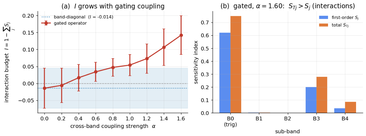
With a fixed sparse clean $\mathbf{c}$, $\sigma =1$, and the detect-then-act gate of Example 1 (coarse band as trigger), Figure 1 averages six replicates at $n=2^{15}$ ($\pm 2$ s.e.).

Remark 4 (Sign and finite-sample behaviour of the estimator). 

The population interaction budget is non-negative, and $I=\frac{1}{V}{\sum }_{\left|u\right|\ge 2}{V}_u\ge 0$ by (2). The pick–freeze estimator $\widehat{I}=1-{\sum }_j{\widehat{S}}_j$, however, is a difference of variance estimators and is not constrained to be non-negative in finite samples: when the true value is $I=0$ (the band-diagonal operator) $\widehat{I}$ fluctuates around 0 with a spread of order $n^{-1/2}$, and small negative values are expected. The reported $I=-0.014\pm 0.030$ lies well within one standard error of 0 and is therefore consistent with $I=0$ under Monte-Carlo error and is not evidence of $I<0$. The estimator is consistent with an $O\left(n^{-1}\right)$ bias from the ratio form; a non-negative reading may be obtained by clipping, ${\widehat{I}}_{+}=max(\widehat{I},0)$ or by estimating ${\sum }_{\left|u\right|\ge 2}{V}_u$ directly, at the cost of introducing a positive bias. We report the raw (unclipped) values throughout to remain faithful to the sampling distribution and to make the $I\approx 0$ null visible.

8.2. Operator/Correlation Separation Under Coloured Noise

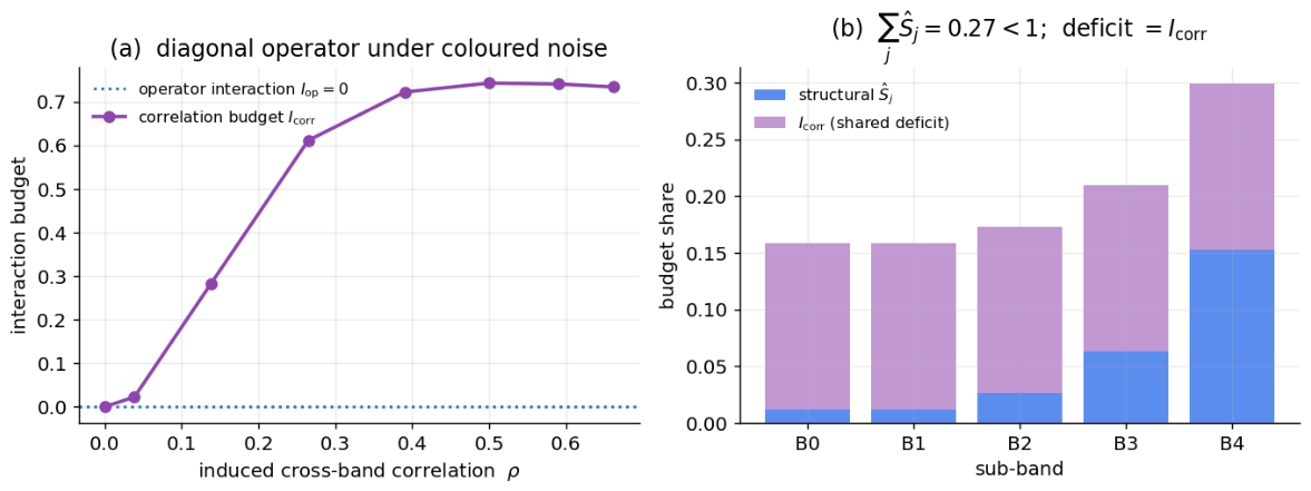
We take a null clean signal $\mathbf{c}=0$, which isolates the noise-correlation mechanism (the worst case); rank-one colour $\xi =\sigma \mathbf{z}+\kappa s\mathbf{1}$, whose shared factor s induces pairwise correlation $\rho ={\kappa }^2/({\sigma }^2+{\kappa }^2)$; and the band-diagonal operator. Figure 2 then reports the resulting split.

8.3. A Realistic ECG Phantom on a Genuine Wavelet Transform

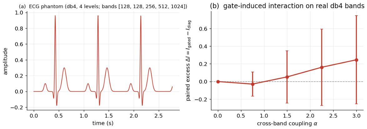
To test the theory on a genuine wavelet transform of a realistic non-stationary biomedical signal, we synthesise a P–QRS–T ECG phantom (heart rate 70 bpm, $f_s=360$ Hz) and decompose it with a genuine orthonormal Daubechies-4 DWT (4 levels, periodisation), giving sub-bands of sizes $(128,128,256,512,1024)$. We add white Gaussian noise, take a coarse band as trigger, and gate the QRS-carrying detail bands. Because the first-order pick–freeze estimator carries a large additive offset on this signal, we report the common-random-number paired excess $\Delta I\left(\alpha \right)=I_{\mathrm{gated}}\left(\alpha \right)-I_{\mathrm{diag}}$, which is exactly 0 at $\alpha =0$ and isolates the operator-induced interaction (4 replicates, $n=2^{13}$). As Figure 3 shows, $\Delta I$ rises from 0 to $\approx 0.25$: the gate induces genuine cross-band interaction on the real db4 sub-bands, exactly as the theory predicts. The phantom isolates the methodology on a fully controlled morphology; the next subsection repeats the test on a genuine measured recording.

8.4. Validation on a Real Measured ECG (MIT-BIH Record 208)

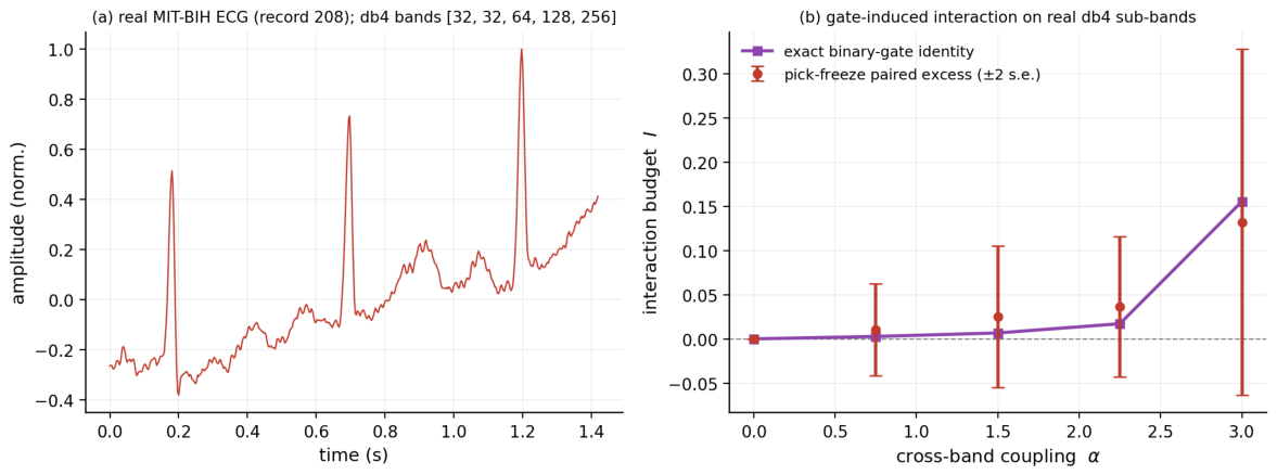
To answer whether the theory holds on genuinely measured—not synthesised—data, we repeat the test on a real recording: a 512-sample window ($\approx 1.4$ s) of MIT-BIH record 208, sampled at 360 Hz [21,22], containing several real QRS complexes and baseline wander. We take a real orthonormal db4 DWT (4 levels, periodisation; sub-band sizes $(32,32,64,128,256)$), add white Gaussian noise at a low SNR ($\sigma =0.7\mathrm{std}$), and apply a binary detect-then-act gate: the coarse band $B_0$ triggers ($p\approx 0.5$) a threshold change on the detail bands. Because the interaction on a strong richly-structured real signal is a small residual of a first-order-dominated variance, we cross-check two independent readings of the same quantity: (i) the exact binary-gate identity $I=\frac{1}{V}{\sum }_{j\ne r}p(1-p)\mathrm{Var}(\Delta g_j)$ of Lemma 2 and (ii) the common-random-number pick–freeze paired excess $\Delta I\left(\alpha \right)=\widehat{I}\left(\alpha \right)-\widehat{I}\left(0\right)$ that cancels the additive offset (6 replicates, $n=2^{13}$). Figure 4 reports both readings.

Two points are worth stating plainly. First, the operator-induced interaction is genuinely smaller on the real high-energy ECG than on the controlled phantom: on richly-structured real signals, the loss variance is dominated by first-order (per-band) noise sensitivity; so, the normalised interaction budget is a modest—though clearly positive and monotone—fraction. This is itself an honest empirical finding about where gating matters. Second, the exact identity and the practical estimator agree; so, a practitioner using only the pick–freeze estimator recovers the same conclusion on real data.

9. Conclusions and Outlook

We developed an exact basis-intrinsic theory of the interaction budget for gated wavelet denoising. The budget I is the $L^2$-distance of the loss to band-additivity: it vanishes if and only if the operator is band-diagonal and otherwise obeys a sharp non-degeneracy condition and a quadratic coupling law. Its second-order EMPR surrogate is exact for single-trigger gates and controllably accurate otherwise, with optimal univariate support functions (Proposition 4) that replace the worst-case curvature by the unexplained gate nonlinearity. Under coloured noise, an EMPR product-support decomposition separates operator-induced from correlation-induced interaction through a correlation-invariant operator signature. Four numerical studies confirm the results: the white-noise interaction budget (Section 8.1), the operator/correlation separation (Section 8.2), a controlled Daubechies-4 ECG phantom (Section 8.3), and a genuine measured MIT-BIH recording (Section 8.4). The separation extends to non-Gaussian colour (Theorem 4): under a finite-copula-density condition it holds verbatim, with the correlation budget expressed through the pairwise band copulas.

9.1. Limitations

Several assumptions delimit the present theory and should temper its use. (i) The framework attributes a scalar performance functional (squared reconstruction error) and, while $\left\{V_{\{j,k\}}\right\}$ localises which scale pairs couple, it does not by itself explain why a gate couples them; it is a diagnostic, not a design rule. (ii) The sharp results of Section 4 and Section 5 assume a single trigger band (Assumption 2); for multi-trigger detectors, only the controllable second-order bound of Proposition 3 applies, and the quadratic law is a small-coupling ($\kappa \to 0$) statement, not a global one. (iii) The correlation core assumes a finite copula density ($\mu \ll {\mu }_{\perp }$); heavy tails or singular dependence that violate this fall outside the guarantees, and $I_{\mathrm{corr}}=0$ does not imply band independence (Theorem 4(iv)). (iv) The pick–freeze estimator is unbiased only asymptotically and is not sign-constrained in finite samples (Remark 4); on strong first-order-dominated real signals, the normalised interaction is small and requires the paired-excess or closed-form readings of Section 8.4 to be resolved cleanly. (v) Our real-data study uses a single-lead ECG record with additive synthetic noise; genuinely non-stationary coloured measurement noise on multi-channel data remains to be tested.

9.2. Future Work

Beyond the data-driven, joint choice of the EMPR support functions of Section 6 across bands, natural extensions are as follows: a real-noise study on multi-record databases (e.g., the MIT-BIH Noise Stress Test set) and on other modalities (reviewer feedback highlighted—bearing and gear vibration and speech—)where transient-preserving gates are common; a sequential/greedy estimator of $I_{\mathrm{op}}$ that exploits the single-trigger structure to reduce the model evaluations; confidence intervals and a non-negative low-bias estimator for I and $I_{\mathrm{corr}}$; an extension of the operator/correlation split to learned gated denoisers (attention and wavelet-decomposition networks [1,2]), turning the interaction budget into a training-time interpretability regulariser; and a decision-theoretic link between the interaction budget and downstream clinical utility, so that “how much coupling” can be tied to “how much diagnostic value is preserved.”

References

1. Jin, Y.; Li, Z.; Tian, Y.; Wei, X.; Liu, C. A novel interpretable multilevel wavelet decomposition deep network for actual heartbeat classification. Sci. China Technol. Sci. 2024, 67, 1842–1854. [Google Scholar] [CrossRef]
2. Edder, A.; Ben-Bouazza, F.E.; Tafala, I.; Manchadi, O.; Jioudi, B. Self Attention-Driven ECG Denoising: A Transformer-Based Approach for Robust Cardiac Signal Enhancement. Signals 2025, 6, 26. [Google Scholar] [CrossRef]
3. Frusque, G.; Fink, O. Robust time series denoising with learnable wavelet packet transform. Adv. Eng. Inform. 2024, 62, 102669. [Google Scholar] [CrossRef]
4. Hoeffding, W. A class of statistics with asymptotically normal distribution. Ann. Math. Stat. 1948, 19, 293–325. [Google Scholar] [CrossRef]
5. Sobol’, I.M. Sensitivity estimates for nonlinear mathematical models. Math. Model. Comput. Exp. 1993, 1, 407–414. [Google Scholar]
6. Jansen, M.J.W. Analysis of variance designs for model output. Comput. Phys. Commun. 1999, 117, 35–43. [Google Scholar] [CrossRef]
7. Saltelli, A.; Annoni, P.; Azzini, I.; Campolongo, F.; Ratto, M.; Tarantola, S. Variance based sensitivity analysis of model output: Design and estimator for the total sensitivity index. Comput. Phys. Commun. 2010, 181, 259–270. [Google Scholar] [CrossRef]
8. Fel, T.; Cadène, R.; Chalvidal, M.; Cord, M.; Vigouroux, D.; Serre, T. Look at the Variance! Efficient Black-box Explanations with Sobol-based Sensitivity Analysis. In Proceedings of the Advances in Neural Information Processing Systems (NeurIPS), Online, 6–14 December 2021. [Google Scholar]
9. Chiogna, G.; Marcolini, G.; Engel, M.; Wohlmuth, B. Sensitivity analysis in the wavelet domain: A comparison study. Stoch. Environ. Res. Risk Assess. 2024, 38, 1669–1684. [Google Scholar] [CrossRef]
10. Tuna, S.; Korkmaz Özay, E.; Tunga, B.; Gürvit, E.; Tunga, M.A. An efficient feature extraction approach for hyperspectral images using Wavelet High Dimensional Model Representation. Int. J. Remote Sens. 2022, 43, 6899–6920. [Google Scholar] [CrossRef]
11. Sudret, B. Global sensitivity analysis using polynomial chaos expansions. Reliab. Eng. Syst. Saf. 2008, 93, 964–979. [Google Scholar] [CrossRef]
12. Mallat, S. A Wavelet Tour of Signal Processing: The Sparse Way, 3rd ed.; Academic Press: Cambridge, MA, USA, 2009. [Google Scholar]
13. Donoho, D.L.; Johnstone, I.M. Ideal spatial adaptation by wavelet shrinkage. Biometrika 1994, 81, 425–455. [Google Scholar] [CrossRef]
14. Rabitz, H.; Aliş, Ö.F. General foundations of high-dimensional model representations. J. Math. Chem. 1999, 25, 197–233. [Google Scholar] [CrossRef]
15. Şen, M.E.; Tuna, S. Exploiting Optimal Supports in Enhanced Multivariance Products Representation for Lossy Compression of Hyperspectral Images. In Proceedings of the 2023 14th International Conference on Electrical and Electronics Engineering (ELECO), Bursa, Turkey, 30 November–2 December 2023; pp. 1–5. [Google Scholar] [CrossRef]
16. Chastaing, G.; Gamboa, F.; Prieur, C. Generalized Hoeffding–Sobol decomposition for dependent variables—Application to sensitivity analysis. Electron. J. Stat. 2012, 6, 2420–2448. [Google Scholar] [CrossRef]
17. Mara, T.A.; Tarantola, S. Variance-based sensitivity indices for models with dependent inputs. Reliab. Eng. Syst. Saf. 2012, 107, 115–121. [Google Scholar] [CrossRef]
18. Kucherenko, S.; Tarantola, S.; Annoni, P. Estimation of global sensitivity indices for models with dependent variables. Comput. Phys. Commun. 2012, 183, 937–946. [Google Scholar] [CrossRef]
19. Owen, A.B. Variance components and generalized Sobol’ indices. SIAM/ASA J. Uncertain. Quantif. 2013, 1, 19–41. [Google Scholar] [CrossRef]
20. Shuvo, S.B.; Alam, S.S.; Ayman, S.U.; Chakma, A.; Salvi, M.; Seoni, S.; Barua, P.D.; Molinari, F.; Acharya, U.R. Application of wavelet transformation and artificial intelligence techniques in healthcare: A systematic review. WIREs Data Min. Knowl. Discov. 2025, 15, e70007. [Google Scholar] [CrossRef]
21. Moody, G.B.; Mark, R.G. The impact of the MIT-BIH Arrhythmia Database. IEEE Eng. Med. Biol. Mag. 2001, 20, 45–50. [Google Scholar] [CrossRef] [PubMed]
22. Goldberger, A.L.; Amaral, L.A.N.; Glass, L.; Hausdorff, J.M.; Ivanov, P.C.; Mark, R.G.; Mietus, J.E.; Moody, G.B.; Peng, C.K.; Stanley, H.E. PhysioBank, PhysioToolkit, and PhysioNet: Components of a new research resource for complex physiologic signals. Circulation 2000, 101, e215–e220. [Google Scholar] [CrossRef] [PubMed]
Figure 1. (a) The band-diagonal operator gives I = 0.014 ± 0.030 0 (shaded). The gated operator’s I rises with a quadratic onset—consistent with Theorem 2: the Δ I α 2 fit on α 0.6 has intercept + 0.0003 —up to 0.142 ± 0.029 at α = 1.6 . (b) Total exceeds first-order ( S T j > S j ) for the trigger band B 0 and the coupled fine bands B 3 , B 4 ; since the gate is single-trigger, all interaction is pairwise with B 0 and E 2 = 0 exactly (Proposition 2).
Mathematics 14 02772 g001
Figure 2. (a) The operator interaction I op 0 at every correlation level (dotted), while the correlation budget I corr rises monotonically with ρ to 0.74 : a correlation-blind reading would misattribute up to 74 % of the variance to operator interaction, but the EMPR split quarantines all of it as correlation. (b) At a representative ρ , j S ^ j = 0.27 < 1 ; the deficit is exactly I corr (estimated identically from 1 j S ^ j and from j k Cov μ ( g j , g k ) / Var μ ( Y ) , confirming I op = 0 ).
Mathematics 14 02772 g002
Figure 3. (a) The synthetic ECG phantom and its genuine db4 sub-band sizes. (b) The common-random-number paired excess Δ I = I gated I diag is 0 at α = 0 by construction and rises with the gate coupling to 0.25 , confirming operator-induced interaction on the real wavelet decomposition (error bars ± 2 s.e.).
Mathematics 14 02772 g003
Figure 4. (a) The real MIT-BIH record 208 window and its genuine db4 sub-band sizes. (b) On the real sub-bands, the interaction budget rises monotonically from 0 with the gate coupling α : the exact binary-gate identity (solid) and the independent pick–freeze paired excess (markers, ± 2 s.e.) agree within error, reaching I 0.16 . The gate induces genuine measurable cross-band interaction on real measured data—confirming the theory beyond synthetic signals; the magnitude is smaller than on the lightweight phantom, because a strong real signal is first-order dominated (Remark 4).
Mathematics 14 02772 g004
Disclaimer/Publisher’s Note: The statements, opinions and data contained in all publications are solely those of the individual author(s) and contributor(s) and not of MDPI and/or the editor(s). MDPI and/or the editor(s) disclaim responsibility for any injury to people or property resulting from any ideas, methods, instructions or products referred to in the content.