Neural Backstepping Control for Trajectory Tracking of Wheeled Mobile Robots

Abstract

This paper presents a Neural Backstepping control strategy for trajectory tracking of a differential-drive mobile robot. The proposed approach combines a dynamic-level backstepping controller with a lightweight single-hidden-layer adaptive neural network to compensate uncertain nonlinear dynamics through online adaptation. The backstepping component provides a Lyapunov-based stabilizing structure, whereas the neural approximator improves tracking performance without requiring deep architectures, offline training stages, or computationally demanding optimization procedures. The adaptive law for the neural output weights is derived from the stability analysis, ensuring bounded closed-loop signals and uniformly ultimately bounded tracking errors in the presence of bounded approximation uncertainties. The controller is evaluated through simulations using four reference trajectories: circular, lemniscate, Lissajous, and waypoint-based paths. The same control gains and neural network configuration are used in all cases, showing that the proposed scheme can track different trajectory geometries without trajectory-specific retuning. The simulation results show satisfactory tracking performance, with position RMSE values below $0.04$ m for all evaluated trajectories. These results indicate that the proposed Neural Backstepping controller provides a suitable balance between tracking accuracy, online adaptation capability, and implementation simplicity for differential-drive mobile robot trajectory tracking.

1. Introduction

Wheeled mobile robots (WMRs) constitute a well-established yet still highly active research platform in autonomous navigation, industrial automation, service robotics, logistics, surveillance, and exploration tasks. Among the available mechanical configurations, differential-drive mobile robots (DDMRs) are widely adopted because of their mechanical simplicity, low cost, maneuverability, and suitability for operation in structured and semi-structured environments. Despite these advantages, accurate trajectory tracking remains a demanding control problem. The difficulty arises from the nonlinear and nonholonomic nature of the system, the coupling between the kinematic and dynamic levels, parametric uncertainty, actuator limitations, external disturbances, wheel–ground interaction effects, and imperfect knowledge of the robot model.

The trajectory-tracking problem consists of designing a control law that forces the robot position and orientation to follow a prescribed reference trajectory while preserving closed-loop stability, acceptable transient behavior, and feasible control inputs. In practical scenarios, these requirements are difficult to satisfy simultaneously because the robot may operate under uncertain or time-varying conditions, including payload variations, friction changes, wheel slip, unmodeled dynamics, bounded disturbances, and actuator-level effects. Therefore, trajectory-tracking controllers for DDMRs should not be evaluated only in terms of nominal tracking-error reduction but also with respect to robustness, adaptability, stability guarantees, tuning complexity, and real-time implementability.

A broad range of nonlinear and intelligent control methodologies has been developed to improve the trajectory-tracking performance of WMRs operating under model uncertainties, disturbances, and nonideal wheel–ground interaction phenomena. Classical nonlinear approaches such as feedback linearization, sliding-mode control, adaptive control, and backstepping have been widely investigated because they explicitly exploit the nonlinear structure of the robot model. Among robust nonlinear methods, sliding-mode control has shown strong disturbance-rejection properties and robustness against parameter variations. For instance, Solea et al. [1] developed a dynamic sliding-mode controller for a unicycle-type wheeled mobile robot subject to bounded uncertainties in mass and inertia, demonstrating accurate trajectory tracking despite significant parametric variations. However, the practical implementation of sliding-mode mechanisms usually requires careful gain selection and may introduce high-frequency control activity when discontinuous compensation terms are used.

Backstepping has received considerable attention because it provides a systematic Lyapunov-based recursive procedure for constructing stabilizing controllers [2]. This feature is particularly relevant for mobile robot trajectory tracking, since the control problem can be naturally organized through a hierarchy involving posture errors, reference velocity commands, and dynamic-level control inputs. In this direction, Ahmadi et al. [3] proposed a state-augmented adaptive backstepping controller that explicitly incorporates actuator dynamics while preserving asymptotic convergence properties. This type of formulation highlights the relevance of dynamic-level backstepping for DDMRs, since purely kinematic controllers may be insufficient when actuator dynamics, inertial effects, and model uncertainties significantly affect the closed-loop response.

Building upon dynamic-level backstepping formulations, several studies have integrated backstepping with robust, sliding-mode, and optimization-based mechanisms. Koubaa et al. [4] proposed an adaptive sliding-mode dynamic control architecture in which a backstepping-based kinematic controller generates the reference velocity commands, whereas the dynamic controller compensates disturbances and parametric uncertainties through a Lyapunov-based design. Huang and Gao [5] combined backstepping with a novel sliding-mode surface to improve convergence rate and robustness with respect to conventional control schemes. Likewise, Qiang et al. [6] developed a cascaded architecture for differential-drive mobile robots, where a backstepping controller regulates the kinematic subsystem and a fractional-order PID controller governs the dynamic subsystem. In that work, the controller parameters are optimized through an improved Grey Wolf Optimization algorithm, obtaining improved IAE and ISE performance indices for complex reference trajectories. These contributions confirm that backstepping is an effective stabilizing backbone; nevertheless, the reported improvements are often achieved by adding sliding-mode terms, fractional-order structures, or metaheuristic optimization layers, which may increase tuning complexity and computational burden.

A complementary line of research has focused on robust and observer-based control strategies for mobile robots subject to slipping, skidding, and external disturbances. Bai et al. [7] addressed trajectory tracking under slipping and skidding effects, emphasizing that wheel–ground interaction can substantially degrade the validity of nominal robot models. Wang et al. [8] combined sliding-mode observers with model predictive control for mecanum-wheeled mobile robots, exploiting disturbance estimation and predictive optimization to improve tracking accuracy. Li et al. [9] proposed an adaptive dual closed-loop controller based on extended-state observers and terminal sliding modes for wheeled mobile robots operating on rough ground. Other recent directions include disturbance-observer-based robust control, prescribed-time control, and data-driven predictive control, which improve disturbance rejection or transient performance under nonideal conditions [10,11,12]. Although these approaches represent important advances in robustness, their implementation may require additional observer layers, stronger assumptions on disturbance bounds, discontinuous control actions, or more elaborate tuning and optimization procedures.

In parallel, neural network-based control has attracted considerable attention because of its capability to approximate unknown nonlinear dynamics and adapt controller parameters online. Rossomando et al. [13] proposed an adaptive neural dynamic compensator that combines feedback linearization with a radial basis function neural network to learn the discrepancy between nominal and actual robot dynamics. A relevant feature of that approach is that the neural network estimates the residual uncertainty rather than the complete system dynamics, thereby reducing the computational burden. Similarly, Ahmine et al. [14] developed an adaptive neural kinematic controller based on an ADALINE neural network combined with a backstepping law, where the neural weights are updated online using the Widrow–Hoff learning rule to improve trajectory-tracking performance under disturbances. Other neural network-based approaches have addressed complementary aspects of mobile robot control, including the explicit handling of velocity constraints and indirect Jacobian identification, improving tracking performance without requiring an exact model or exhaustive manual tuning [15,16]. These works show that neural compensation can improve robustness and adaptability; however, purely kinematic compensation or indirect neural identification may be insufficient when uncertain dynamic effects, actuator-level behavior, and persistent modeling errors have a dominant influence on the closed-loop response.

More recently, hybrid architectures combining backstepping, neural networks, adaptive control, and intelligent optimization have been investigated for mobile robot trajectory tracking. Hassan and Saleem [17] proposed a neural network-based adaptive controller integrated with a model reference adaptive control framework to improve tracking in the presence of parameter uncertainties, wheel-slip disturbances, and measurement noise. Dang et al. [18] designed an adaptive backstepping hierarchical sliding-mode controller using radial basis function neural networks for three-wheeled mobile robots and integrated it with A* global path planning and a Timed Elastic Band local planner for obstacle avoidance. Ha and Than [19] introduced a neural backstepping adaptive controller in which the neural network adjusts the backstepping parameters online to compensate longitudinal and lateral wheel slip. Arega et al. [20] combined backstepping with a neural network-based nonlinear PID controller, showing improved tracking accuracy and robustness with respect to conventional PID and nonlinear PID schemes. These studies highlight the potential of neural-enhanced backstepping architectures under uncertain operating conditions. Nevertheless, improved adaptability is frequently obtained at the cost of additional control layers, planning modules, indirect tuning mechanisms, or neural structures that may be less attractive for resource-constrained embedded platforms.

Reinforcement learning-assisted and data-driven control strategies have also expanded the scope of mobile robot trajectory tracking. He et al. [21] proposed a self-adaptive Double Q-backstepping scheme in which reinforcement learning is used to tune controller parameters under varying operating conditions. Data-driven predictive control based on Koopman-operator modeling has also been explored to improve the representation of nonlinear robot dynamics within a model predictive control framework [12]. These methods are promising because they can improve adaptability and generalization beyond fixed-gain nonlinear controllers. However, their practical use may involve offline learning requirements, data-dependent modeling, optimization stages, or computationally demanding prediction mechanisms. As discussed in recent studies on mobile robot motion planning and reinforcement learning-based architectures, the increasing incorporation of learning methods into robotic control improves flexibility but also raises concerns regarding stability guarantees, interpretability, real-time feasibility, and implementation complexity [10].

Recent advances in adaptive learning control further illustrate the increasing interest in combining nonlinear control with learning-based adaptation. Fixed-time hierarchical game-based schemes have been investigated for coordinated unmanned aerial–ground vehicle systems [22], while behavior-guided adaptive dynamic programming has been proposed for neural learning control under adjustable behavioral objectives [23]. These developments are relevant because they show the potential of learning mechanisms to improve adaptability in complex nonlinear systems. At the same time, they also reinforce a central practical issue: learning-enhanced controllers must balance adaptability with stability guarantees, architectural simplicity, and computational feasibility. For DDMRs, this balance is particularly important because the controller is often expected to run online on embedded hardware while compensating uncertain nonlinear dynamics.

Lightweight adaptive neural controllers have emerged as a relevant alternative for reducing the gap between adaptability and implementability. Lima et al. [24] proposed an adaptive neural controller for omnidirectional mobile robots subject to unmodeled dynamics, showing that compact neural approximators can improve tracking accuracy while maintaining feasible computational demands. This direction is particularly important for embedded robotic systems, where the controller must remain sufficiently simple for real-time execution. Nevertheless, neural approximation alone is not sufficient for stability-sensitive trajectory tracking. The neural component must be embedded within a rigorous nonlinear control design capable of guaranteeing bounded closed-loop behavior.

The preceding analysis shows that the state of the art has advanced along two main directions. On the one hand, robust nonlinear and observer-based controllers provide strong stability and disturbance-rejection properties, but they may require additional observers, discontinuous terms, complex tuning procedures, or accurate knowledge of uncertainty bounds. On the other hand, neural, reinforcement learning, adaptive learning, and data-driven controllers improve adaptability and approximation capability, but they may rely on deeper architectures, offline training stages, additional optimization layers, data-dependent modeling, or computational resources that are not always compatible with real-time embedded implementation. Consequently, an open research gap remains in the development of trajectory-tracking controllers for DDMRs that simultaneously provide a rigorous Lyapunov-based stability structure, online compensation of uncertain nonlinear dynamics, low computational complexity, and direct suitability for real-time implementation without trajectory-specific retuning or offline neural training.

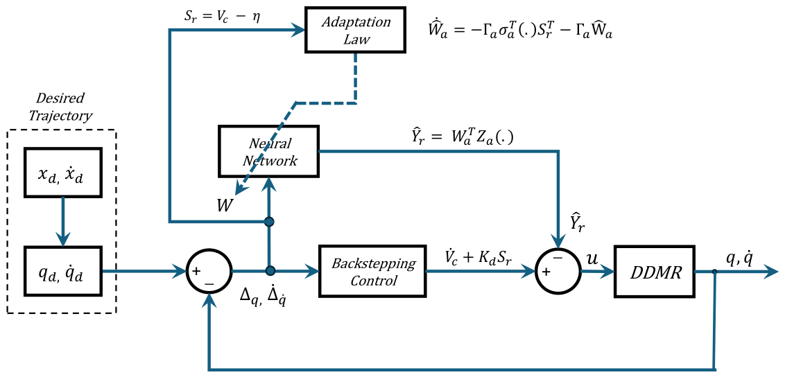
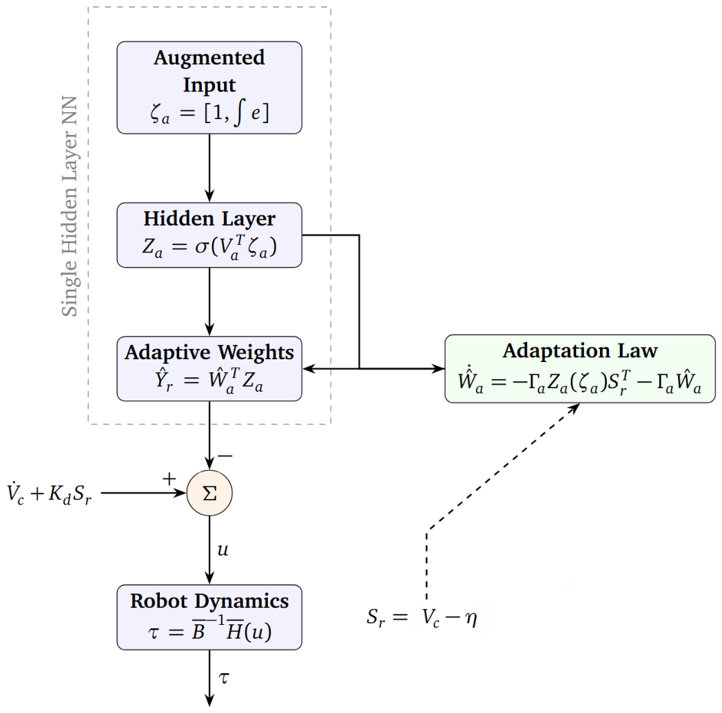
Motivated by this gap, this paper proposes a Neural Backstepping control strategy for trajectory tracking of a differential-drive mobile robot. The proposed method combines a dynamic-level backstepping controller with a lightweight single-hidden-layer adaptive neural network. The backstepping component provides the stabilizing structure of the control law, whereas the neural component compensates uncertain nonlinear dynamics through online adaptation. Unlike more computationally intensive learning-based approaches, the proposed neural approximator is intentionally kept compact in order to preserve real-time implementability while maintaining sufficient approximation capability for control purposes.

The main contribution of this work is the integration of a Lyapunov-based dynamic backstepping controller with a compact adaptive neural approximator for uncertain DDMR trajectory tracking. In contrast with robust schemes that rely primarily on observer layers or discontinuous compensation terms, the proposed controller incorporates the neural network output directly into the auxiliary control law associated with the computed-torque structure. In contrast with learning-based approaches that require offline training, deeper architectures, or additional optimization stages, the neural output weights are updated online through an adaptation law derived from the Lyapunov stability analysis. In this manner, the controller is designed to improve trajectory-tracking accuracy, compensate persistent modeling errors, and maintain bounded closed-loop signals in the presence of bounded approximation uncertainties.

The specific contributions of this paper are summarized as follows:

• A dynamic-level Neural Backstepping control scheme is formulated for trajectory tracking of a differential-drive mobile robot, combining the recursive stabilizing structure of backstepping with online neural compensation of uncertain nonlinear dynamics.
• A lightweight single-hidden-layer adaptive neural network is integrated into the auxiliary computed-torque control law, avoiding deep architectures, offline training stages, and additional optimization layers commonly used in several learning-based controllers.
• A Lyapunov-based adaptation law is derived for the neural output weights, ensuring boundedness of the closed-loop signals and uniformly ultimately bounded tracking errors under bounded approximation uncertainties.
• The proposed controller is evaluated through numerical simulations using different reference trajectories, and its tracking performance is analyzed in terms of position errors, orientation error, and control response.

The remainder of this paper is organized as follows. Section 2 presents the kinematic and dynamic models of the differential-drive mobile robot, including the reduced representation used for control design. Section 3 develops the proposed Neural Backstepping control strategy, the adaptive neural approximator, and the stability analysis. Section 4 presents the simulation setup, trajectory-tracking results, and discussion of the controller performance. Finally, Section 5 summarizes the main conclusions and outlines future research directions.

2. Differential-Drive Mobile Robot Model

This section presents the kinematic and dynamic model of the DDMR considered in this work. The model is formulated in terms of the robot pose, the wheel angular velocities, and the admissible velocity subspace imposed by the nonholonomic constraints. This representation is later used to derive the proposed Neural Backstepping controller.

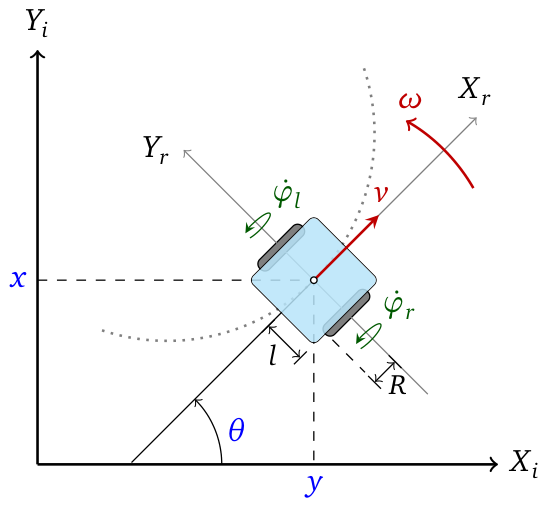
The robot under study, represented in Figure 1 by a model in the $xy$ plane, is a nonholonomic mechanical system consisting of a rigid body (base) with four wheels: two conventional fixed wheels driven by independent electric actuators through DC motors for motion and orientation, and two additional passive wheels that rotate freely, providing stability and support during movement, in a (2,0)-type robot configuration [25]. The effect of the passive wheels on the dynamics of the DDMR is considered negligible and, therefore, is not taken into account in the mathematical development of this research [26].

The robot’s pose vector is represented by the triplet $\xi = {[x, y, \theta ]}^T$. Figure 1 illustrates the geometric configuration and the main variables of the differential-drive mobile robot. The coordinates $(x,y)$ denote the position of the robot in the inertial reference frame $\{O,X_i,Y_i\}$, while $\theta$ represents its orientation angle with respect to the $X_i$ axis. The variables v and $\omega$ correspond to the linear and angular velocities of the robot, respectively. The wheel radius is denoted by R, and $2l$ represents the distance between the driving wheels. The angular velocities of the right and left wheels are represented by ${\dot{\varphi }}_r$ and ${\dot{\varphi }}_l$, respectively. These variables establish the relationship between the wheel motions and the robot kinematics used in the controller design. The parameters of the DDMR model are described in

Table 1. DDMR parameters.

Parameter	Description
A	Intersection of the symmetry axis with the wheel axis and the center of mass or orientation point
R	Radius of the left and right wheels
$2l$	Distance between the actuated wheels and the symmetry axis
$m_c$	Mass of the DDMR without motors and wheels
$m_w$	Mass of each wheel motor assembly
$m_t$	Total mass of the DDMR
$I_c$	Moment of inertia of the DDMR without wheels or motors with respect to the vertical axis passing through point A
$I_w$	Moment of inertia of each wheel and motor with respect to the wheel axis
$I_m$	Moment of inertia of each wheel and motor about the vertical axis parallel to the wheel plane
I	Total moment of inertia of the DDMR
${\dot{\varphi }}_r,{\dot{\varphi }}_l$	Angular velocity of the right and left wheels
$\upsilon ,\omega$	Linear and angular velocities of the DDMR

.

The local coordinates of the vehicle’s mechanical system can be described in terms of the generalized coordinate vector $q = {[q_1, q_2, \dots , q_n]}^{\top }$. The motion of the mechanical system is subject to various constraints that must be satisfied at all times during operation.

These constraints take the form of algebraic relationships between the positions and velocities of the system’s points and are incorporated into the kinematic model of the differential-drive robot.

2.1. Kinematic Model of the DDMR

The kinematic model of the differential robot is referenced to a fixed inertial frame $\{O,X_i,Y_i\}$. The linear (v) and angular ($\omega$) velocities of the robot are determined by the following forward differential kinematic relationship:

$$\begin{array}{cc}\hfill v& =\dot{x}cos\left(\theta \right)+\dot{y}sin\left(\theta \right),\hfill \\ \hfill \omega & =\dot{\theta }.\hfill \end{array}$$

(1)

The inverse relationship of the previous expressions, in matrix form, is given by the equation that defines the kinematic model of the DDMR, that is,

$$\left[\begin{array}{c}\dot{x}\\ \dot{y}\\ \dot{\theta }\end{array}\right]=\left[\begin{array}{cc}cos\theta & 0\\ sin\theta & 0\\ 0& 1\end{array}\right]\left[\begin{array}{c}v\\ \omega \end{array}\right],$$

(2)

Assumption 1.

For the kinematic analysis of the differential-drive vehicle, the following conditions are assumed: the robot moves over a flat surface free from level and texture irregularities; the motion axes are parallel to the working surface; robot slippage during movement is neglected; and the robot structure is considered completely rigid, and thus, no flexible components are taken into account in the design.

The linear and angular velocities of the DDMR are defined as functions of the angular velocities of each wheel as follows:

$$\upsilon \left(t\right)={\displaystyle \frac{\left({\dot{\phi }}_r+{\dot{\phi }}_l\right)R}{2}},$$

(3)

$$\omega \left(t\right)={\displaystyle \frac{\left({\dot{\phi }}_r-{\dot{\phi }}_l\right)R}{2l}}.$$

(4)

The DDMR shown in Figure 1 presents three kinematic constraints [27]. The first establishes that lateral slipping is not allowed (no-slip constraint), whereas the remaining two correspond to wheel rotation (pure-rolling constraints). These constraints are described as follows:

$$\begin{array}{cc}\hfill \dot{y}cos\left(\theta \right)-\dot{x}sin\left(\theta \right)& =0,\hfill \\ \hfill \dot{x}cos\left(\theta \right)+\dot{y}sin\left(\theta \right)+l\dot{\theta }-R{\dot{\phi }}_r& =0,\hfill \\ \hfill \dot{x}cos\left(\theta \right)+\dot{y}sin\left(\theta \right)-l\dot{\theta }-R{\dot{\phi }}_l& =0,\hfill \end{array}$$

(5)

where (${\dot{\phi }}_r$ and ${\dot{\phi }}_l$) represent the angular velocities of the right and left wheels, respectively.

It is worth noting that the kinematic constraints (5) are linear relationships with the generalized coordinate vector $q = {\left[\begin{array}{ccccc}x& y& \theta & {\phi }_r& {\phi }_l\end{array}\right]}^{\top }$ and can be represented by the expression

$$A\left(q\right)\dot{q}=0,$$

(6)

where the Pfaffian matrix (annihilator of the generalized velocities) is given by

$$A\left(q\right)=\left[\begin{array}{ccccc}-sin\theta & cos\theta & 0& 0& 0\\ cos\theta & sin\theta & l& -R& 0\\ cos\theta & sin\theta & -l& 0& -R\end{array}\right].$$

(7)

Likewise, there exists an orthogonal projection ($S\left(q\right)\in {\mathbb{R}}^{m\times n}$) of the Pfaffian matrix, whose span is the kernel of A. The Jacobian defined by

$$S\left(q\right)={\displaystyle \frac{1}{2}}\left[\begin{array}{cc}Rcos\theta & Rcos\theta \\ Rsin\theta & Rsin\theta \\ R/l& -R/l\\ 2& 0\\ 0& 2\end{array}\right],$$

(8)

acts as an annihilator of the constraints in (7) and is composed of a set of linearly independent vector fields distributed within the null space of $A\left(q\right)$.

The relationship between $A\left(q\right)$ and $S\left(q\right)$ is expressed by

$$A\left(q\right)S\left(q\right)=0,$$

(9)

which is a property that will be used to simplify the robot’s dynamics.

For the design of trajectory-tracking and obstacle-avoidance algorithms for small vehicles, considering only kinematics is sufficient. However, when the vehicle’s weight and load capacity are substantial, motion dynamics must be considered.

2.2. The Dynamic Model of the DDMR

The dynamic model of a differential mobile robot describes the motion of the system considering both the internal (endogenous) and external (exogenous) forces acting on it. The internal forces are associated with the actuators and the mechanical interaction between the robot’s components, such as the torques applied by the motors to the wheels and the mass distribution of the system. On the other hand, the external forces include environmental effects such as friction with the surface, slopes along the path, contact forces with obstacles, and other disturbances. Dynamic analysis makes it possible to accurately describe the behavior of the robot, which is essential for the design of robust and efficient controllers, in contrast to kinematics, which only analyzes motion without considering forces (velocities and positions, among others) [28].

The dynamic model of the DDMR, with n generalized coordinates $(q_1, q_2, \dots , q_n)$ and m constraints, can be represented as

$$H\left(q\right)\ddot{q}+C(q,\dot{q})\dot{q}+{\tau }_d=B\left(q\right)\tau -A^T\left(q\right)\lambda ,$$

(10)

where $H\left(q\right)$ is the positive-definite, symmetric $n \times n$ inertia matrix; $C(q,\dot{q})$ is the centripetal and Coriolis matrix; and ${\tau }_d$ is an $n \times 1$ vector that denotes uncertainties and disturbances, including modeling inaccuracies, surface friction, external disturbances, unknown bounded disturbances, unmodeled and unstructured dynamics of actuators, sensors and other electronic devices, integration errors, noise, and operational sampling and physical limitations, where for the analysis presented in this work, it is taken to be equal to zero. $B\left(q\right)$ is the input matrix, $\tau$ is the input vector, $A^T\left(q\right)$ is the matrix associated with the kinematic constraints, and $\lambda$ is the vector of Lagrange multipliers. The dynamic Equation (10) of the DDMR does not include the gravitational force, since the vehicle is assumed to move only on flat, level surfaces. Equation (10) has the following properties:

Property 1

(Boundedness). The inertia matrix $H\left(q\right)$, the norm of the Coriolis and centrifugal matrix $C(q,\dot{q})$, and the disturbance vector ${\tau }_d$ are bounded.

Property 2

(Skew-symmetry). The matrix $\dot{H}\left(q\right)-2C(q,\dot{q})$ is skew-symmetric.

Property 3

(Passivity). The energy supplied by the control inputs is bounded by the variation in the system’s total energy, yielding

$${\int }_{t_0}^{t_f}{\tau }^T\dot{q}dt=E\left(t_f\right)-E\left(t_0\right)\ge -E\left(t_0\right),\forall t_f\ge t_0.$$

(11)

These properties are important in the stability analysis of the control system.

2.2.1. Euler–Lagrange Dynamic Modeling

The Euler–Lagrange approach is a fundamental tool in the dynamic formulation of mechanical systems, since it allows the derivation of the equations of motion from energetic considerations of the system. This method, developed by Lagrange, is used to systematically derive the equations of motion by considering the kinetic and potential energies of the given system [28]. The Lagrange equation can be written as

$${\displaystyle \frac{d}{dt}}\left({\displaystyle \frac{\partial L}{\partial \dot{q_i}}}\right)-{\displaystyle \frac{\partial L}{\partial q_i}}=\mathit{F}-{\mathit{A}}^{\mathit{T}}\left(q\right)\lambda ,$$

(12)

where $L = T - V$ is the Lagrangian function; T is the kinetic energy and V the potential energy of the system; $q_i$ is generalized coordinates; F is the generalized force vector; $A\left(q\right)$ is an $m \times n$ matrix associated with the nonholonomic constraints of the DDMR, where n is the number of generalized coordinates $(q_1, q_2, \dots , q_n)$ and m the number of constraints; and $\lambda$ is the vector of Lagrange multipliers associated with the constraints.

To develop the dynamic model of the vehicle, the equations that describe the different components of the Lagrange function are established. Since the potential energy is zero due to the motion of the vehicle on a horizontal plane without a slope, it can be stated that $L = T$ [27].

The total kinetic energy of the DDMR is the sum of the kinetic energy of the vehicle platform and that of the wheels and actuators.

The kinetic energy of the vehicle platform is

$$T_c={\displaystyle \frac{1}{2}}{m}_c{{\upsilon }_c}^2+{\displaystyle \frac{1}{2}}{I}_c{\dot{\theta }}^2,$$

(13)

whereas the kinetic energy of the right and left wheels are

$$\begin{array}{c}\hfill T_{{\omega }_r}={\displaystyle \frac{1}{2}}{m}_{\omega }{{\upsilon }_{{\omega }_r}}^2+{\displaystyle \frac{1}{2}}{I}_m{\dot{\theta }}^2+{\displaystyle \frac{1}{2}}{I}_{\omega }{\dot{{\phi }_r}}^2\\ \hfill T_{{\omega }_l}={\displaystyle \frac{1}{2}}{m}_{\omega }{{\upsilon }_{{\omega }_l}}^2+{\displaystyle \frac{1}{2}}{I}_m{\dot{\theta }}^2+{\displaystyle \frac{1}{2}}{I}_{\omega }{\dot{{\phi }_l}}^2,\end{array}$$

(14)

where $m_c$ is the mass of the DDMR without the driving wheels and actuators, $m_{\omega }$ is the mass of each driving wheel (with actuator), $I_c$ is the moment of inertia of the DDMR with respect to the vertical axis that passes through the center of mass, $I_{\omega }$ is the moment of inertia of each driving wheel with motor with respect to the axis of the wheel, and $I_m$ is the moment of inertia of each driving wheel with motor with respect to the diameter of the wheel. The coordinates $(x_a,y_a)$ of the center of mass and the wheels can be obtained in terms of the generalized coordinates as follows:

$$\begin{array}{cc}\hfill x_{{\omega }_r}& =x_a+lsin\theta ,\hfill \\ \hfill y_{{\omega }_r}& =y_a-lcos\theta ,\hfill \\ \hfill x_{{\omega }_l}& =x_a-lsin\theta ,\hfill \\ \hfill y_{{\omega }_l}& =y_a+lcos\theta .\hfill \end{array}$$

(15)

Adding (13) and (14), and substituting (15), the total kinetic energy of the DDMR can be written as

$$T={\displaystyle \frac{1}{2}}m\left({\dot{x_a}}^2+{{\dot{y}}_a}^2\right)+{\displaystyle \frac{1}{2}}{I}_{\omega }({\dot{{\phi }_r}}^2+{\dot{{\phi }_l}}^2)+{\displaystyle \frac{1}{2}}I{\dot{\theta }}^2,$$

(16)

where $m = m_c + 2m_{\omega }$ is the total mass of the vehicle and $I = I_c + 2m_{\omega }{l}^2+2I_m$ is the equivalent total inertia. The Lagrangian is given by $L = T - V$, where the potential energy is $V = 0$ since the DDMR operates in the $(x,y)$ plane. Solving (12), the following inertia and Coriolis matrices are obtained:

$$H\left(q\right)\left(\ddot{q}\right)=\mathrm{diag}\left([m,m,I,I_{\omega },I_{\omega }]\right),$$

(17)

$$C(q,\dot{q})\dot{q}=0_{5\times 5},$$

(18)

together with the input matrix

$$B\left(q\right)=\left[\begin{array}{cc}0& 0\\ 0& 0\\ 0& 0\\ 1& 0\\ 0& 1\end{array}\right].$$

(19)

Consequently, the Lagrangian model becomes

$$H\left(q\right)\ddot{q}=B\left(q\right)\tau -A^T\left(q\right)\lambda .$$

(20)

The model described by (20) represents the Lagrangian dynamics of the DDMR moving on a plane, without considering friction in the actuator shaft and the wheels. The latter aspect will be set aside without loss of generality, since both friction effects are endogenous and additive and therefore can be included in future work.

The DDMR model developed is an underactuated model, since it has five generalized coordinates but only two actuators that directly affect the angular velocity of the driving wheels. This characteristic implies that not all state variables can be directly controlled, which represents a significant challenge in the design of control strategies, while at the same time realistically reflecting the physical limitations of the system.

The dynamics of the differential-drive mobile robot (DDMR) defined by (20) describe the behavior of the system by explicitly considering the nonholonomic constraints through the use of Lagrange multipliers. However, for control and simulation purposes, it is more convenient to rewrite the system within its subspace of admissible solutions, that is, in the set of motions that inherently satisfy the imposed constraints.

2.2.2. Dynamics of the DDMR Within a Solution Subspace

By integrating the system (20) into its solution space defined by the constraints, it becomes a more suitable representation for control and simulation purposes.

If we define the reduced vector $\eta$, which encompasses the linear and angular velocity components of the differential drive mobile robot (DDMR), as

$$\eta =\left[\begin{array}{c}v\\ w\end{array}\right],$$

(21)

then, to rewrite the system within its subspace of admissible solutions, that is, the set of motions that inherently satisfy the imposed constraints, it is necessary to introduce a matrix $S\left(q\right)$ whose columns span the null space of the Pfaffian constraint matrix $A\left(q\right)$, such that

$$S^T\left(q\right)A^T\left(q\right)=0.$$

(22)

In accordance with the expression of $S\left(q\right)$ shown in (8), it can be verified that it satisfies condition (22) by computing the transposes of both matrices and performing the corresponding operation.

Therefore, the constrained forward differential kinematics is given by

$$\dot{q}=S\left(q\right)\eta ,$$

(23)

where $\dot{q} = {\left[\dot{x}\dot{y}\dot{\theta }{\dot{\phi }}_r{\dot{\phi }}_l\right]}^T$. By differentiating (23), one obtains the constrained forward acceleration kinematics,

$$\ddot{q}=\dot{S}\left(q\right)\eta +S\left(q\right)\dot{\eta },$$

(24)

which can be incorporated into the dynamic Equation (20). Subsequently, by multiplying this equation by $S{\left(q\right)}^T$, the dynamic system is projected onto the admissible subspace of motions, explicitly eliminating the Lagrange multipliers $\lambda$. This operation yields reduced embedded dynamics, expressed solely in terms of the actuated variables contained in the reduced vector $\eta$ (21), considering the expressions (3) and (4); this is intrinsically compatible with the system constraints.

This reformulation not only reduces the computational complexity of the model but also lays the foundation for the design of control strategies based on the system dynamics, without the need to handle the constraints directly, since these have been absorbed into the structure of the model.

Therefore, by substituting (23) and (24) into (20), multiplying the result by $S{\left(q\right)}^T$, and rearranging the terms, the embedded dynamics in reduced form can be obtained as

$$\overline{H}\left(q\right)\dot{\eta }+\overline{C}\left(q,\dot{q}\right)\eta =\overline{B}\left(q\right)\tau ,$$

(25)

in which the corresponding terms are given by

$$\begin{array}{ccc}\hfill \overline{H}& =& S^T\left(q\right)H\left(q\right)S\left(q\right)\hfill \\ & =& \left[\begin{array}{cc}m+{\displaystyle \frac{2I_{\omega }}{R^2}}& 0\\ 0& I+{\displaystyle \frac{2l^2{I}_{\omega }}{R^2}}\end{array}\right];\hfill \end{array}$$

(26)

$$\begin{array}{ccc}\hfill \overline{C}& =& S^T\left(q\right)H\left(q\right)\dot{S}\left(q\right)\hfill \\ & =& \left[\begin{array}{cc}0& 0\\ 0& 0\end{array}\right];\hfill \end{array}$$

(27)

$$\begin{array}{ccc}\hfill \overline{B}\left(q\right)& =& S^T\left(q\right)B\left(q\right)\hfill \\ & =& \left[\begin{array}{cc}{\displaystyle \frac{1}{R}}& {\displaystyle \frac{1}{R}}\\ {\displaystyle \frac{l}{R}}& -{\displaystyle \frac{l}{R}}\end{array}\right].\hfill \end{array}$$

(28)

The system (25) expresses the dynamics of the DDMR on the tangent bundle of the manifold defined by $S\left(q\right)$; more precisely, the motion is described as a function of the linear and angular velocity components of the differential drive mobile robot $(v,w)$ controlled by the motor torques $({\tau }_r,{\tau }_l)$.

Hence, there appears to be tangent bundle dynamics of the DDMR over the manifold $S\left(q\right)$, showing the 2-DoF actuated reachable dynamics in terms of input motor torques $({\tau }_r,{\tau }_l)$ of the right and left wheels.

$$\overline{H}\left(q\right)\overline{B}{\left(q\right)}^{-1}\dot{\eta }=\tau +{\overline{\tau }}_d$$

(29)

where velocity $\eta = {\left[\dot{p}\dot{\theta }\right]}^T = {\left[v\omega \right]}^T$, for $p = \left(xy\right)$, stands for the state and $\tau = {\left[{\tau }_r{\tau }_l\right]}^T$ the control input.

3. Proposed Neural Backstepping Control

The proposed control system is based on the Backstepping control strategy described by Khalil [29] and incorporates an adaptive neural network. These approaches are integrated, and the resulting control action is applied to the DDMR through the control input u. Figure 2 presents the overall architecture of the proposed Neural Backstepping control scheme. The desired trajectory generator provides the reference position and velocity signals used to compute the tracking errors. The backstepping controller processes these errors to generate the commanded velocity vector. The adaptive neural network operates in parallel to estimate uncertain nonlinear dynamics and compensate for modeling inaccuracies through online adaptation of the output-layer weights. Finally, the resulting control action is applied to the robot dynamic model, closing the feedback loop and enabling trajectory-tracking performance under uncertain conditions.

3.1. Backstepping Control

To design the controller, given the robot’s size and weight, it is necessary to consider not only its kinematics but also its dynamics. Therefore, a control scheme similar to that developed by [30] is employed, but with a different kinematic and dynamic model and with constraints specific to the differential-drive robot.

For this purpose, it is necessary to consider an auxiliary control input u within the computed torque control, which is derived from the reduced dynamic model

$$\begin{array}{cc}\hfill \tau & =\overline{B}{\left(q\right)}^{-1}\overline{H}\left(q\right)\dot{\eta },\hfill \\ \hfill \dot{q}& =S\left(q\right)\eta ,\hfill \end{array}$$

(30)

In order to formulate the control law directly in terms of the physical actuation variables, the control input is defined as the vector of wheel torques,

$$\tau =\left[\begin{array}{c}{\tau }_r\\ {\tau }_l\end{array}\right],$$

(31)

where ${\tau }_r$ and ${\tau }_l$ represent the torques applied to the right and left wheels, respectively. Considering the reduced dynamic model, the expression (30) can be reformulated as follows:

$$\dot{\eta }=\overline{H}{\left(q\right)}^{-1}\overline{B}\left(q\right)\tau .$$

(32)

The expression (32) represents a control architecture that utilizes the torque inputs provided by each motor, which are subsequently regulated through a Backstepping Control strategy. This control is a step-by-step (“back-step”) controller that begins with a portion of the system (typically the one closest to the output) and then proceeds backward, adding dynamics and designing virtual control variables until the final control input is obtained. Its objective is to track trajectories point-by-point, given the following desired (reference) velocities and positions:

$$\begin{array}{cc}\hfill {\dot{x}}_d& =v_{d}cos\left({\theta }_d\right),\hfill \\ \hfill {\dot{y}}_d& =v_{d}sin\left({\theta }_d\right),\hfill \\ \hfill {\dot{\theta }}_d& ={\omega }_d,\hfill \\ \hfill q_d& ={\left[\begin{array}{ccc}{x}_d& y_d& {\theta }_d\end{array}\right]}^T,\hfill \\ \hfill V_d& ={\left[\begin{array}{cc}{v}_d& {\omega }_d\end{array}\right]}^T.\hfill \end{array}$$

(33)

To develop the Backstepping control, we build upon the work of [30,31,32] for the Backstepping controller and [33] for the Actor-type Neural control. This methodology is adapted to the specific dynamic model of the robot under study, given by (25). Accordingly, it is necessary to present the desired (reference) positions and velocities in matrix form:

$$\left[\begin{array}{c}{\dot{x}}_d\\ {\dot{y}}_d\\ {\dot{\theta }}_d\end{array}\right]=\left[\begin{array}{cc}cos{\theta }_d& 0\\ sin{\theta }_d& 0\\ 0& 1\end{array}\right]\left[\begin{array}{c}{v}_d\\ {\omega }_d\end{array}\right].$$

(34)

To enable the robot to follow a predefined trajectory determined by the desired positions and orientation ${[x_d,y_d,{\theta }_d]}^T$, it is necessary to determine the tracking error. This error is defined as the difference between the desired position and the robot’s current position, not in global coordinates, but within the robot’s own reference frame. This approach enables the control system to accurately estimate the robot’s forward distance to the target, its lateral deviation, and the angular difference between its orientation and the target orientation. To incorporate these deviations within the robot’s frame, they must be expressed by multiplying by a transformation matrix that maps the error from the global frame to the robot frame, as given by

$$e=\left[\begin{array}{c}{e}_x\\ e_y\\ e_{\theta }\end{array}\right]=\left[\begin{array}{ccc}cos\left(\theta \right)& sin\left(\theta \right)& 0\\ -sin\left(\theta \right)& cos\left(\theta \right)& 0\\ 0& 0& 1\end{array}\right]\left[\begin{array}{c}{x}_d-x\\ y_d-y\\ {\theta }_d-\theta \end{array}\right].$$

(35)

where $e_x$, $e_y$, and $e_{\theta }$ denote the longitudinal, lateral, and orientation tracking errors expressed in the robot reference frame. This rotation matrix transforms the error from the global inertial frame to the robot’s local frame. This change of coordinates simplifies the controller design, as the control laws can be formulated directly in the robot frame.

Given that the controller’s objective is to drive the tracking error $(e_x,e_y,e_{\theta })$ to zero, it is essential to determine its temporal evolution by differentiating (35), yielding the following expression for the time derivative of the error $e = {[e_x, e_y, e_{\theta }]}^T$:

$$\dot{e}=\left[\begin{array}{c}{\dot{e}}_x\\ {\dot{e}}_y\\ {\dot{e}}_{\theta }\end{array}\right]=\left[\begin{array}{c}\omega e_y-v+v_{d}cos\left(e_{\theta }\right)\\ -\omega e_x+v_{d}sin\left(e_{\theta }\right)\\ {\omega }_d-\omega \end{array}\right],$$

(36)

where ${\dot{e}}_x = \omega e_y - v + v_{d}cos\left(e_{\theta }\right)$ is the forward error, which varies depending on the robot’s advance relative to the desired trajectory; ${\dot{e}}_y = -\omega e_x + v_{d}sin\left(e_{\theta }\right)$ is the lateral error, which changes due to the robot’s orientation and turning rate; and ${\dot{e}}_{\theta } = {\omega }_d - \omega$ is the angular error that represents the difference between the desired orientation and the current one. Since the goal is for the errors to converge to zero in a stable manner, exponentially decaying desired dynamics (stabilization via linear feedback) are proposed:

$$\begin{array}{cc}\hfill {\dot{e}}_x& =-k_x{e}_x,\hfill \\ \hfill {\dot{e}}_y& =-k_y{e}_y,\hfill \\ \hfill {\dot{e}}_{\theta }& =-k_{\theta }{e}_{\theta },\hfill \end{array}$$

(37)

where $k_x$, $k_y$, and $k_{\theta }$ are positive gains that determine the rate at which the errors converge to zero. In the desired angular error dynamics, $e_{\theta }$ is replaced by $sin \left(e_{\theta }\right)$ because this increases robustness against large orientation errors. For small orientation errors, using the approximation $sin \left(e_{\theta }\right) \approx e_{\theta }$, the dynamics exhibit linear behavior.

Since the goal is to define a control velocity $V_c = f_c(e,V_d,k)$, the kinematic tracking error dynamics are used to construct the commanded velocity to be applied in the control system. Accordingly, the control velocity is proposed as

$$V_c=\left[\begin{array}{c}{v}_c\\ {\omega }_c\end{array}\right]=\left[\begin{array}{c}{v}_{d}cos\left(e_{\theta }\right)+k_x{e}_x\\ {\omega }_d+v_d\left(k_y{e}_y+k_{\theta }sin\left(e_{\theta }\right)\right)\end{array}\right].$$

(38)

The control law in (38) is selected based on a Lyapunov analysis in order to guarantee the stability of the tracking error dynamics. Consider the candidate Lyapunov function

$$V={\displaystyle \frac{1}{2}}(e_x^2+e_y^2)+{\displaystyle \frac{1-cos\left(e_{\theta }\right)}{k_y}},$$

(39)

which is positive definite for $k_y > 0$, since $V > 0$ for $e \ne 0$ and $V = 0$ when $e = 0$.

Its time derivative is given by

$$\dot{V}=e_x{\dot{e}}_x+e_y{\dot{e}}_y+{\displaystyle \frac{sin\left(e_{\theta }\right)}{k_y}}{\dot{e}}_{\theta }.$$

(40)

Using the kinematic error dynamics

$${\dot{e}}_x=\omega e_y-v+v_{d}cos\left(e_{\theta }\right),{\dot{e}}_y=-\omega e_x+v_{d}sin\left(e_{\theta }\right),{\dot{e}}_{\theta }={\omega }_d-\omega ,$$

(41)

it follows that

$$\dot{V}=e_x\left(\omega e_y-v+v_{d}cos\left(e_{\theta }\right)\right)+e_y\left(-\omega e_x+v_{d}sin\left(e_{\theta }\right)\right)+{\displaystyle \frac{sin\left(e_{\theta }\right)}{k_y}}({\omega }_d-\omega ).$$

(42)

Finally, by substituting $v = v_c$ and $\omega = {\omega }_c$ from (38), the Lyapunov derivative becomes

$$\dot{V}=-k_x{e}_x^2-{\displaystyle \frac{v_d{k}_{\theta }}{k_y}}{sin}^2\left(e_{\theta }\right)\le 0.$$

(43)

Since the Lyapunov derivative is negative semidefinite, the closed-loop kinematic error system is stable in the Lyapunov sense. Furthermore, under standard assumptions on the reference velocity $V_d$, asymptotic convergence can be established by invoking LaSalle’s invariance principle. Based on expression (30), the following auxiliary control equation is proposed:

$$u=\dot{V_c}+K_d(V_c-\eta )$$

(44)

Differentiating (38), the time derivative of the commanded velocity vector is obtained as follows:

$${\dot{V}}_c=\left[\begin{array}{c}{\dot{v}}_c\\ {\dot{\omega }}_c\end{array}\right]=\left[\begin{array}{c}{\dot{v}}_{d}cos\left(e_{\theta }\right)-v_{d}sin\left(e_{\theta }\right){\dot{e}}_{\theta }+k_x{\dot{e}}_x\\ {\dot{\omega }}_d+{\dot{v}}_d\left(k_y{e}_y+k_{\theta }sin\left(e_{\theta }\right)\right)+v_d\left(k_y{\dot{e}}_y+k_{\theta }cos\left(e_{\theta }\right){\dot{e}}_{\theta }\right)\end{array}\right].$$

(45)

With (44) substituted into (30), the torque control law associated with the Backstepping controller is fully specified:

$$\tau =\overline{B}{\left(q\right)}^{-1}\overline{H}\left(q\right)(\dot{V_c}+K_d(V_c-\eta )).$$

(46)

The term ${\dot{V}}_c$ provides the feedforward component required to follow the time-varying virtual velocity command, whereas the feedback term $K_d(V_c-\eta )$ introduces damping into the velocity error dynamics.

In this way, the computed-torque term compensates for the reduced robot dynamics, while the backstepping feedback term ensures convergence of the actual velocity vector toward the virtual velocity command.

For interpretation purposes, an auxiliary acceleration-like signal may be defined as

$$u={\dot{V}}_c+K_{\eta }\left(V_c-\eta \right).$$

(47)

Thus, the torque law can be compactly written as

$$\tau =\overline{B}{\left(q\right)}^{-1}\overline{H}\left(q\right)u.$$

(48)

It is important to emphasize that u is only an internal auxiliary signal with acceleration units, whereas the actual control input applied to the robot is the torque vector $\tau$.

3.2. Adaptive Neural Network Approximator

The neural component incorporated into the proposed controller is formulated as a single-hidden-layer feedforward neural network, which serves as an adaptive approximator of the uncertain system dynamics [34,35]. The employed architecture utilizes nonlinear basis functions in the hidden layer in conjunction with adaptively updated weights in the output layer, as illustrated in Figure 3.

The control objective is to ensure that $V_c\to \eta$ as $t\to \infty$, which implies that the commanded velocities converge to the actual velocities. To improve robustness against model uncertainties and unmodeled dynamics, the neural network estimate ${\widehat{Y}}_r$ is incorporated into the auxiliary control law as

$$u={\dot{V}}_c+K_d(V_c-\eta )-{\widehat{Y}}_r,$$

(49)

where the velocity tracking error is defined as

$$S_r=V_c-\eta .$$

(50)

The input vector of the neural approximator is defined as

$${\zeta }_a=\left[\begin{array}{c}1\\ \int e_{x}dt\\ \int e_{y}dt\\ \int e_{\theta }dt\end{array}\right]\in {\mathbb{R}}^4,$$

(51)

where the constant entry equal to one allows the hidden-layer bias to be absorbed into the fixed weight matrix.

The hidden-layer output is given by

$$Z_a\left({\zeta }_a\right)={\sigma }_a\left(V_a^T{\zeta }_a\right)\in {\mathbb{R}}^a,$$

(52)

where ${\zeta }_a$ denotes the neural network input vector, $V_a\in {\mathbb{R}}^{4\times a}$ is the fixed hidden-layer weight matrix, a is the number of hidden neurons, and ${\sigma }_a(·)$ is the activation function.

According to the neural network approximation property, the uncertain nonlinear function can be represented as

$$Y_r\left({\zeta }_a\right)=W_a^{\top }{Z}_a\left({\zeta }_a\right)+{\epsilon }_a\left({\zeta }_a\right),$$

(53)

where $Z_a\left({\zeta }_a\right)$ represents the hidden-layer activation vector, $W_a\in {\mathbb{R}}^{a\times 2}$ denotes the ideal output weight matrix, and ${\epsilon }_a\left({\zeta }_a\right)$ is the bounded approximation error. Therefore, the neural estimate is chosen as

$${\widehat{Y}}_r={\widehat{W}}_a^T{Z}_a\left({\zeta }_a\right),$$

(54)

where ${\widehat{W}}_a\in {\mathbb{R}}^{a\times 2}$ is the adaptive output-layer weight matrix [34].

Substituting the neural estimate into the auxiliary control law yields

$$u={\dot{V}}_c+K_d{S}_r-{\widehat{W}}_a^T{Z}_a\left({\zeta }_a\right).$$

(55)

Hence, the torque control law of the Neural Backstepping approach is given by

$$\tau ={\overline{B}}^{-1}\overline{H}\left({\dot{V}}_c+K_d{S}_r-{\widehat{Y}}_r\right).$$

(56)

The neural network output and the corresponding adaptation law are defined as follows:

$${\widehat{Y}}_r={\widehat{W}}_a^T{Z}_a\left({\zeta }_a\right),$$

(57)

$${\dot{\widehat{W}}}_a=-{\Gamma }_a{Z}_a\left({\zeta }_a\right)S_r^T-{\Gamma }_a{\widehat{W}}_a,$$

(58)

where ${\Gamma }_a\in {\mathbb{R}}^{a\times a}$ is a positive definite adaptation gain matrix.

3.3. Stability Analysis for the Control System with Backstepping and an Adaptive Neural Network

To analyze the stability properties of the proposed Neural Backstepping controller, define the velocity tracking error as

$$S_r=V_c-\eta ,$$

(59)

where $\eta = {\left[v\omega \right]}^T$ denotes the actual velocity vector and $V_c = {\left[v_c{\omega }_c\right]}^T$ is the commanded velocity vector generated by the kinematic Backstepping stage.

The auxiliary control input is selected as

$$u={\dot{V}}_c+K_d{S}_r-{\widehat{Y}}_r,$$

(60)

where $K_d\in {\mathbb{R}}^{2\times 2}$ is a symmetric positive definite gain matrix and ${\widehat{Y}}_r$ is the neural network estimate of the normalized uncertain dynamics. Hence, the torque control law is given by

$$\tau ={\overline{B}}^{-1}\overline{H}\left({\dot{V}}_c+K_d{S}_r-{\widehat{Y}}_r\right).$$

(61)

After applying the computed-torque transformation, the closed-loop dynamics can be written in normalized form as

$$\dot{\eta }=u+Y_r,$$

(62)

where $Y_r$ denotes the normalized uncertain nonlinear dynamics.

The input vector of the neural approximator is defined as

$${\zeta }_a=\left[\begin{array}{c}1\\ \int e_{x}dt\\ \int e_{y}dt\\ \int e_{\theta }dt\end{array}\right]\in {\mathbb{R}}^4,$$

(63)

where the constant entry equal to one allows the hidden-layer bias to be absorbed into the fixed weight matrix. The hidden-layer output is given by

$$Z_a\left({\zeta }_a\right)={\sigma }_a\left(V_a^T{\zeta }_a\right)\in {\mathbb{R}}^a,$$

(64)

with $V_a\in {\mathbb{R}}^{4\times a}$ denoting the fixed hidden-layer weight matrix and ${\sigma }_a(·)$ the activation function.

According to the neural network approximation property, the uncertain nonlinear function can be represented as

$$Y_r\left({\zeta }_a\right)=W_a^{\top }{Z}_a\left({\zeta }_a\right)+{ϵ}_a\left({\zeta }_a\right),$$

(65)

where $W_a\in {\mathbb{R}}^{a\times 2}$ is the ideal output weight matrix and ${ϵ}_a\left({\zeta }_a\right)\in {\mathbb{R}}^2$ is the bounded approximation error. The neural estimate is chosen as

$${\widehat{Y}}_r={\widehat{W}}_a^T{Z}_a\left({\zeta }_a\right),$$

(66)

where ${\widehat{W}}_a\in {\mathbb{R}}^{a\times 2}$ is the adaptive output-layer weight matrix. Define the weight estimation error as

$${\tilde{W}}_a=W_a-{\widehat{W}}_a.$$

(67)

Since $S_r = V_c-\eta$, its time derivative satisfies

$${\dot{S}}_r={\dot{V}}_c-\dot{\eta }.$$

(68)

Substituting the normalized dynamics and the auxiliary control law yields

$$\begin{array}{cc}\hfill {\dot{S}}_r& ={\dot{V}}_c-\left({\dot{V}}_c+K_d{S}_r-{\widehat{Y}}_r+Y_r\right)\hfill \\ \hfill & =-K_d{S}_r-{\tilde{W}}_a^T{Z}_a\left({\zeta }_a\right)-{ϵ}_a\left({\zeta }_a\right).\hfill \end{array}$$

(69)

Consider the Lyapunov candidate function

$$V={\displaystyle \frac{1}{2}}{S}_r^T{S}_r+{\displaystyle \frac{1}{2}}\mathrm{tr}\left({\tilde{W}}_a^T{\Gamma }_a^{-1}{\tilde{W}}_a\right),$$

(70)

where ${\Gamma }_a\in {\mathbb{R}}^{a\times a}$ is a symmetric positive definite adaptation gain matrix. Its time derivative is

$$\dot{V}=S_r^T{\dot{S}}_r+\mathrm{tr}\left({\tilde{W}}_a^T{\Gamma }_a^{-1}{\dot{\tilde{W}}}_a\right).$$

(71)

Substituting the error dynamics gives

$$\dot{V}=-S_r^T{K}_d{S}_r-S_r^T{\tilde{W}}_a^T{Z}_a\left({\zeta }_a\right)-S_r^T{ϵ}_a\left({\zeta }_a\right)+\mathrm{tr}\left({\tilde{W}}_a^T{\Gamma }_a^{-1}{\dot{\tilde{W}}}_a\right).$$

(72)

The adaptive law is selected as

$${\dot{\widehat{W}}}_a=-{\Gamma }_a{Z}_a\left({\zeta }_a\right)S_r^T-{\Gamma }_a{\widehat{W}}_a,$$

(73)

where the second term corresponds to a leakage ($\sigma$-modification) component introduced to guarantee bounded adaptive weights.

Since $W_a$ is assumed constant,

$${\dot{\tilde{W}}}_a=-{\dot{\widehat{W}}}_a={\Gamma }_a{Z}_a\left({\zeta }_a\right)S_r^T+{\Gamma }_a{\widehat{W}}_a.$$

(74)

Using ${\widehat{W}}_a = W_a-{\tilde{W}}_a$, it follows that

$${\dot{\tilde{W}}}_a={\Gamma }_a{Z}_a\left({\zeta }_a\right)S_r^T+{\Gamma }_a{W}_a-{\Gamma }_a{\tilde{W}}_a.$$

(75)

Therefore,

$$\begin{array}{cc}\hfill \mathrm{tr}\left({\tilde{W}}_a^T{\Gamma }_a^{-1}{\dot{\tilde{W}}}_a\right)& =\mathrm{tr}\left({\tilde{W}}_a^T{Z}_a\left({\zeta }_a\right)S_r^T\right)+\mathrm{tr}\left({\tilde{W}}_a^T{W}_a\right)-\mathrm{tr}\left({\tilde{W}}_a^T{\tilde{W}}_a\right)\hfill \\ \hfill & =S_r^T{\tilde{W}}_a^T{Z}_a\left({\zeta }_a\right)+\mathrm{tr}\left({\tilde{W}}_a^T{W}_a\right)-{\parallel {\tilde{W}}_a\parallel }_F^2.\hfill \end{array}$$

(76)

Hence,

$$\dot{V}=-S_r^T{K}_d{S}_r-S_r^T{ϵ}_a\left({\zeta }_a\right)+\mathrm{tr}\left({\tilde{W}}_a^T{W}_a\right)-{\parallel {\tilde{W}}_a\parallel }_F^2.$$

(77)

Using

$$S_r^T{ϵ}_a\left({\zeta }_a\right)\le \parallel S_r\parallel \parallel {ϵ}_a\left({\zeta }_a\right)\parallel ,$$

(78)

and

$$\mathrm{tr}\left({\tilde{W}}_a^T{W}_a\right)\le {\displaystyle \frac{1}{2}}\parallel {\tilde{W}}_a{\parallel }_F^2+{\displaystyle \frac{1}{2}}{\parallel W_a\parallel }_F^2,$$

(79)

one obtains

$$\dot{V}\le -{\lambda }_{min}\left(K_d\right)\parallel S_r{\parallel }^2-{\displaystyle \frac{1}{2}}\parallel {\tilde{W}}_a{\parallel }_F^2+\parallel S_r\parallel \parallel {ϵ}_a\left({\zeta }_a\right)\parallel +{\displaystyle \frac{1}{2}}{\parallel W_a\parallel }_F^2.$$

(80)

If the approximation error is bounded as

$$\parallel {ϵ}_a\left({\zeta }_a\right)\parallel \le {\overline{ϵ}}_a,$$

(81)

then, by Young’s inequality,

$$\parallel S_r\parallel {\overline{ϵ}}_a\le {\displaystyle \frac{{\lambda }_{min}\left(K_d\right)}{2}}{\parallel S_r\parallel }^2+{\displaystyle \frac{{\overline{ϵ}}_a^2}{2{\lambda }_{min}\left(K_d\right)}}.$$

(82)

Thus,

$$\dot{V}\le -{\displaystyle \frac{{\lambda }_{min}\left(K_d\right)}{2}}\parallel S_r{\parallel }^2-{\displaystyle \frac{1}{2}}\parallel {\tilde{W}}_a{\parallel }_F^2+{\displaystyle \frac{{\overline{ϵ}}_a^2}{2{\lambda }_{min}\left(K_d\right)}}+{\displaystyle \frac{1}{2}}{\parallel W_a\parallel }_F^2.$$

(83)

Therefore, the Lyapunov derivative is negative outside a compact set. It follows that all closed-loop signals remain bounded and that both the velocity tracking error $S_r$ and the weight estimation error ${\tilde{W}}_a$ are uniformly ultimately bounded (UUB). Consequently, the proposed Neural Backstepping controller guarantees practical stability in the presence of bounded neural approximation errors and the leakage term included in the adaptation law.

4. Simulation Results and Discussion

This section presents a numerical evaluation of the proposed Neural Backstepping controller for trajectory tracking of a differential-drive mobile robot. Rather than considering a single nominal trajectory, the controller is tested on four reference paths with different geometric and dynamic characteristics: circular, lemniscate, Lissajous, and waypoint-based trajectories. This selection allows the closed-loop response to be analyzed under constant-curvature motion, curvature reversals, multi-frequency oscillatory behavior, and piecewise transitions between waypoints. Therefore, the simulation study is intended to assess not only the tracking accuracy of the proposed controller but also its transient response, control effort, and ability to operate without trajectory-specific retuning.

4.1. Simulation Setup

The simulations were carried out in MATLAB/Simulink R2024a using the reduced dynamic model of the DDMR and the proposed Neural Backstepping control law. The closed-loop scheme integrates the robot dynamics, the trajectory generator, the body-frame tracking-error computation, the adaptive neural approximator, and the torque control input.

All simulations were conducted using a sampling period of $T_s = 0.01 \mathrm{s}$. The initial pose of the robot was set to

$$\xi \left(0\right)={\left[\begin{array}{ccc}x\left(0\right)& y\left(0\right)& \theta \left(0\right)\end{array}\right]}^T={\left[\begin{array}{ccc}0& 0& 0\end{array}\right]}^T.$$

(84)

The physical parameters of the robot used in the simulations are summarized as follows:

$$m=27 \mathrm{k}\mathrm{g},I=2.0336 \mathrm{k}\mathrm{g} {\mathrm{m}}^2,I_w=0.0201 \mathrm{k}\mathrm{g} {\mathrm{m}}^2,$$

(85)

$$R=0.1016 \mathrm{m},l=0.3282 \mathrm{m}.$$

(86)

The same controller configuration was used for all evaluated trajectories. The backstepping gains were selected as

$$k_x=2,k_y=3,k_{\theta }=2,$$

(87)

and the dynamic feedback gain was defined as

$$K_d=\mathrm{diag}(2,2).$$

(88)

The adaptive neural network was implemented with 10 hidden neurons. The adaptive output-weight matrix satisfies

$${\widehat{W}}_a\in {\mathbb{R}}^{10\times 2},$$

(89)

whereas the fixed hidden-layer matrix is

$$V_a\in {\mathbb{R}}^{4\times 10}.$$

(90)

The hidden-layer basis vector is given by

$$Z_a\left({\zeta }_a\right)={\sigma }_a\left(V_a^T{\zeta }_a\right)\in {\mathbb{R}}^{10},$$

(91)

where ${\sigma }_a(·)$ denotes a bipolar sigmoid activation function. The neural network input vector is defined as

$${\zeta }_a={\left[\begin{array}{cccc}1& \int e_{x}dt& \int e_{y}dt& \int e_{\theta }dt\end{array}\right]}^T,$$

(92)

where the neural network input vector is composed of the integral tracking errors and a constant bias term. The adaptation gain was selected as

$${\Gamma }_a=80I_{10},$$

(93)

where $I_{10}$ is the identity matrix of dimension 10 × 10.

In the simulations, the hidden-layer matrix $V_a$ was fixed a priori, while only the output-layer weights ${\widehat{W}}_a$ were adapted online. Therefore, the role of $V_a$ is to generate a sufficiently rich nonlinear feature mapping for the adaptive approximation, rather than being adjusted during the learning process. The fixed hidden-layer weights were initialized once from a uniform distribution,

$${\left[V_a\right]}_{ij}\sim \mathcal{U}(-1,1),$$

(94)

and remained unchanged during each simulation. This bounded initialization range was selected to provide sufficient variation among the bipolar sigmoid basis functions while avoiding excessive activation saturation. Fixing $V_a$ preserves the linear parameterization of the neural approximator with respect to the output weights, which is required by the proposed adaptation law and the Lyapunov stability analysis. Therefore, only the output-layer matrix ${\widehat{W}}_a$ was updated online.

4.2. Sensitivity Analysis of the Number of Hidden Neurons

A sensitivity analysis was performed to determine an appropriate hidden-layer size for the adaptive neural network. Architectures with $a\in \{6, 8, 10, 12, 14\}$ hidden neurons were evaluated using the four reference trajectories. The robot parameters, initial conditions, sampling time, controller gains, activation function, weight initialization procedure, and adaptation law were kept unchanged. For each architecture, the adaptation gain was defined as ${\Gamma }_a = 80I_a$, where $I_a$ is the identity matrix of dimension a.

For a network with a hidden neurons, the dimensions of the fixed hidden-layer matrix and the adaptive output-layer matrix are

$$V_a\in {\mathbb{R}}^{4\times a},{\widehat{W}}_a\in {\mathbb{R}}^{a\times 2}.$$

Consequently, the number of output weights updated online is $2a$.

Table 2. Sensitivity analysis of the number of hidden neurons. The best result for each tracking metric is shown in bold.

Hidden Neurons	Circle	Lemniscate	Lissajous	Waypoints	Average Position	Average Orientation	Adaptive
a	RMSE [m]	RMSE [m]	RMSE [m]	RMSE [m]	RMSE [m]	RMSE [rad]	Weights
6	0.035420	0.014615	0.023531	0.043920	0.029372	0.033171	12
8	0.032184	0.012468	0.020219	0.039476	0.026087	0.029687	16
10	0.030857	0.011373	0.018842	0.036999	0.024518	0.027593	20
12	0.031286	0.011816	0.019296	0.037648	0.025012	0.028122	24
14	0.032041	0.012327	0.019987	0.038741	0.025774	0.028923	28

presents the position RMSE obtained for each trajectory, the average position and orientation RMSE values, and the corresponding number of adaptive output weights.

Increasing the number of hidden neurons from 6 to 10 progressively reduced the tracking errors. The 10-neuron network achieved the lowest position RMSE for each reference trajectory and the lowest average orientation RMSE among all evaluated architectures. Compared with the six-neuron architecture, the average position RMSE decreased from 0.029372 m to 0.024518 m, corresponding to a reduction of approximately 16.5%.

Increasing the hidden-layer size to 12 or 14 neurons did not improve the tracking performance. Relative to the 10-neuron configuration, the average position RMSE increased by approximately 2.0% and 5.1%, respectively, while the number of adaptive output weights increased from 20 to 24 and 28. Therefore, 10 hidden neurons were selected as the best trade-off between nonlinear approximation capability, tracking accuracy, and online adaptation complexity.

4.3. Reference Trajectories and Controller Parameters

Four reference trajectories were considered to evaluate the behavior of the proposed controller. The circular and Lissajous trajectories were selected to assess the transient response when the robot starts away from the desired path. The lemniscate trajectory was considered to evaluate smooth tracking along a continuous closed path. Finally, the waypoint-based trajectory was included to analyze the controller response under piecewise path changes and sharper curvature transitions.

The same controller gains and neural network configuration were used in all cases. This is relevant because no gain retuning was required when changing from smooth closed curves to the waypoint-based path. Therefore, the results provide evidence that the proposed Neural Backstepping strategy can successfully track different reference patterns using a single control configuration.

4.4. Trajectory-Tracking Performance

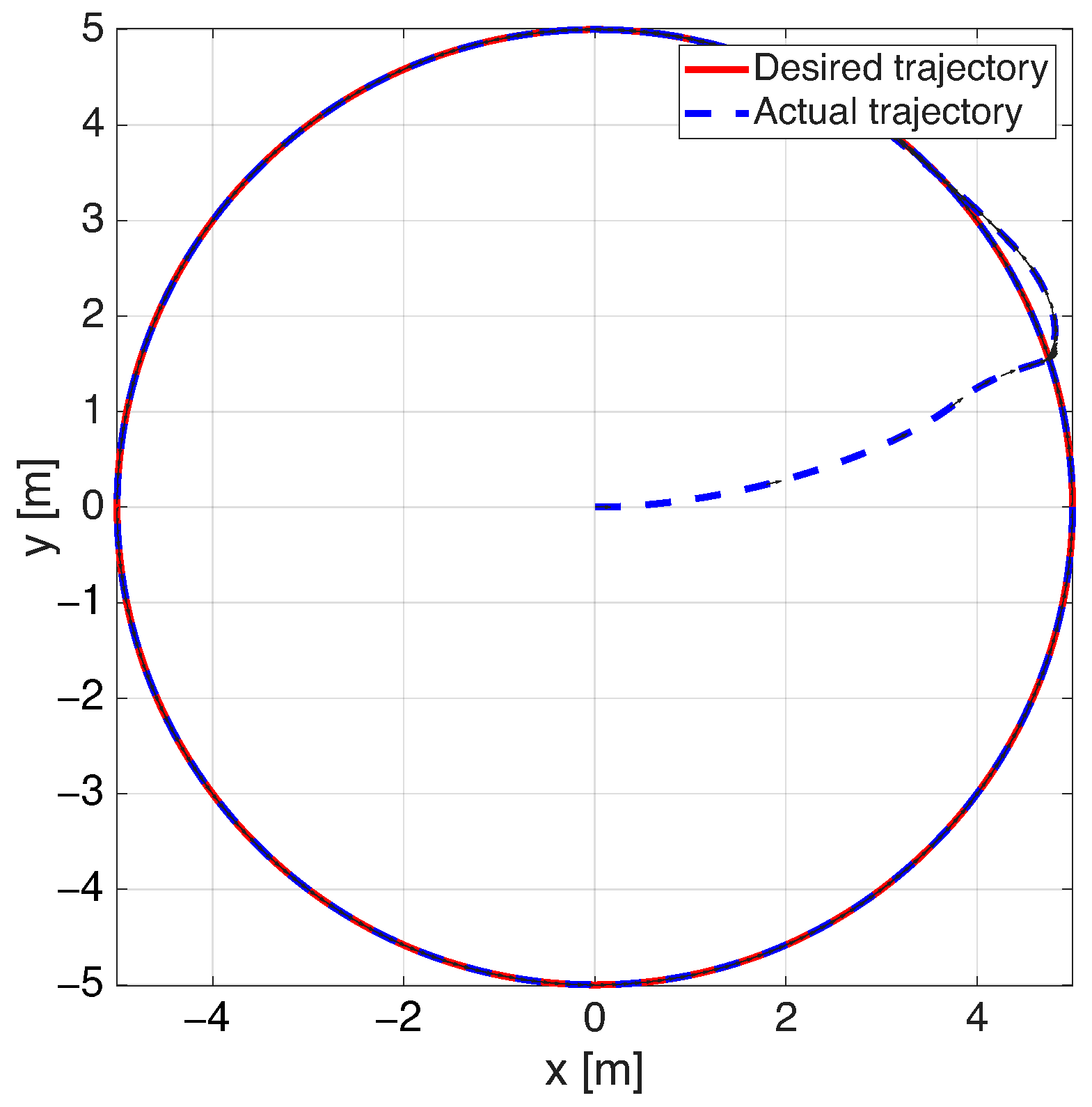
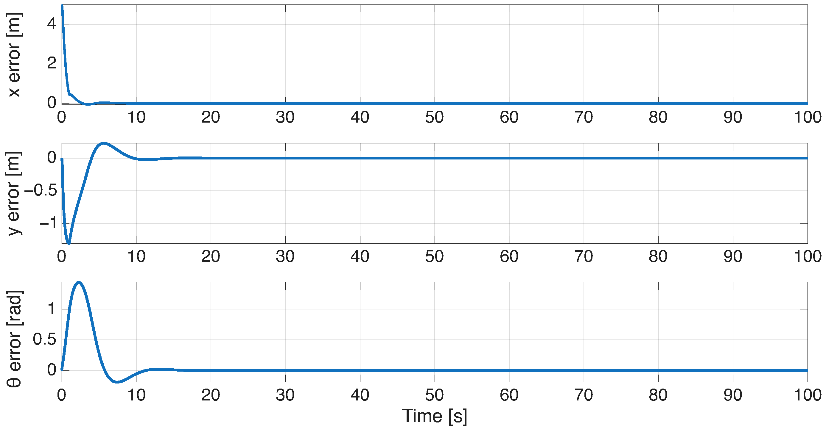
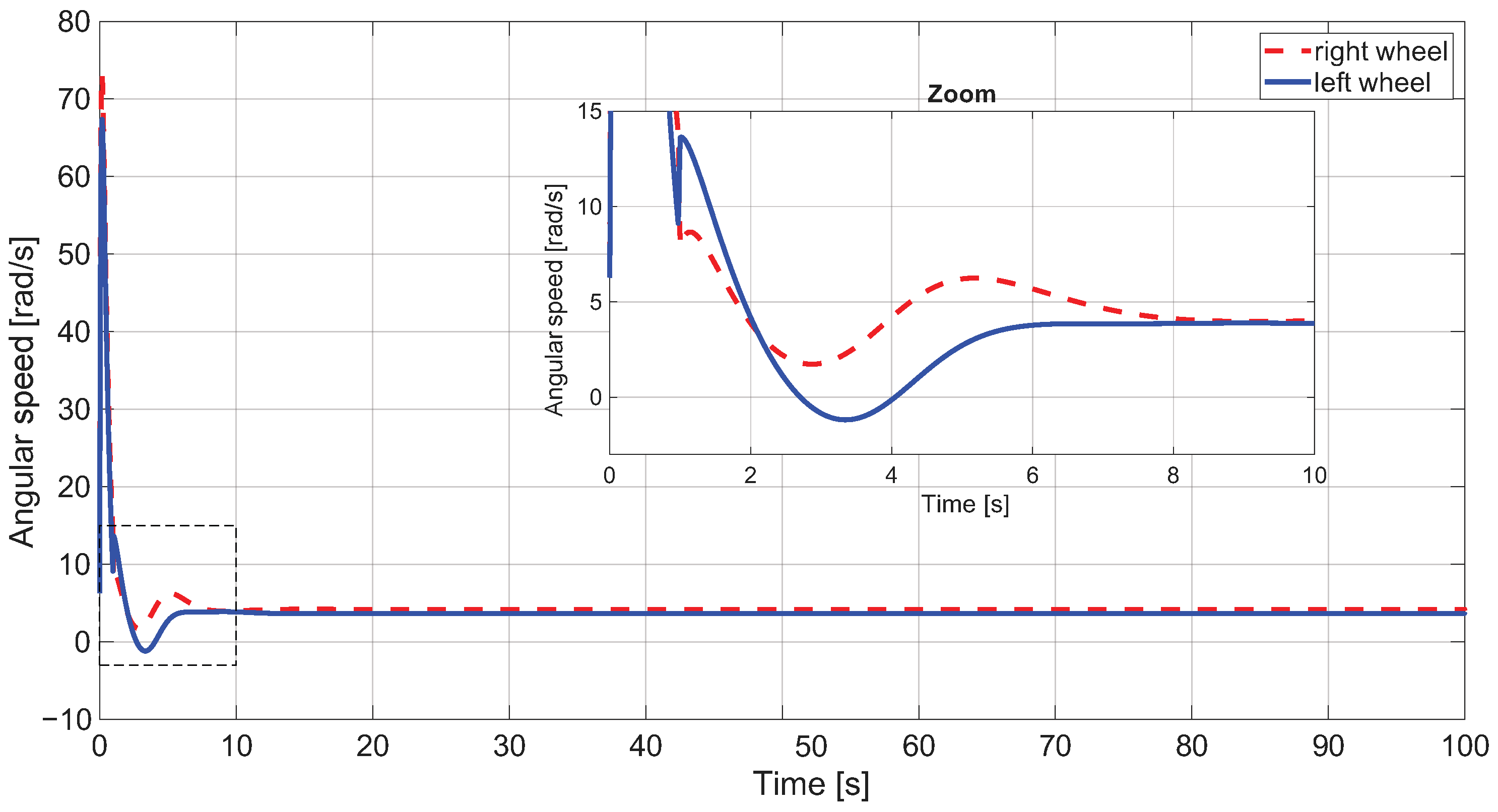
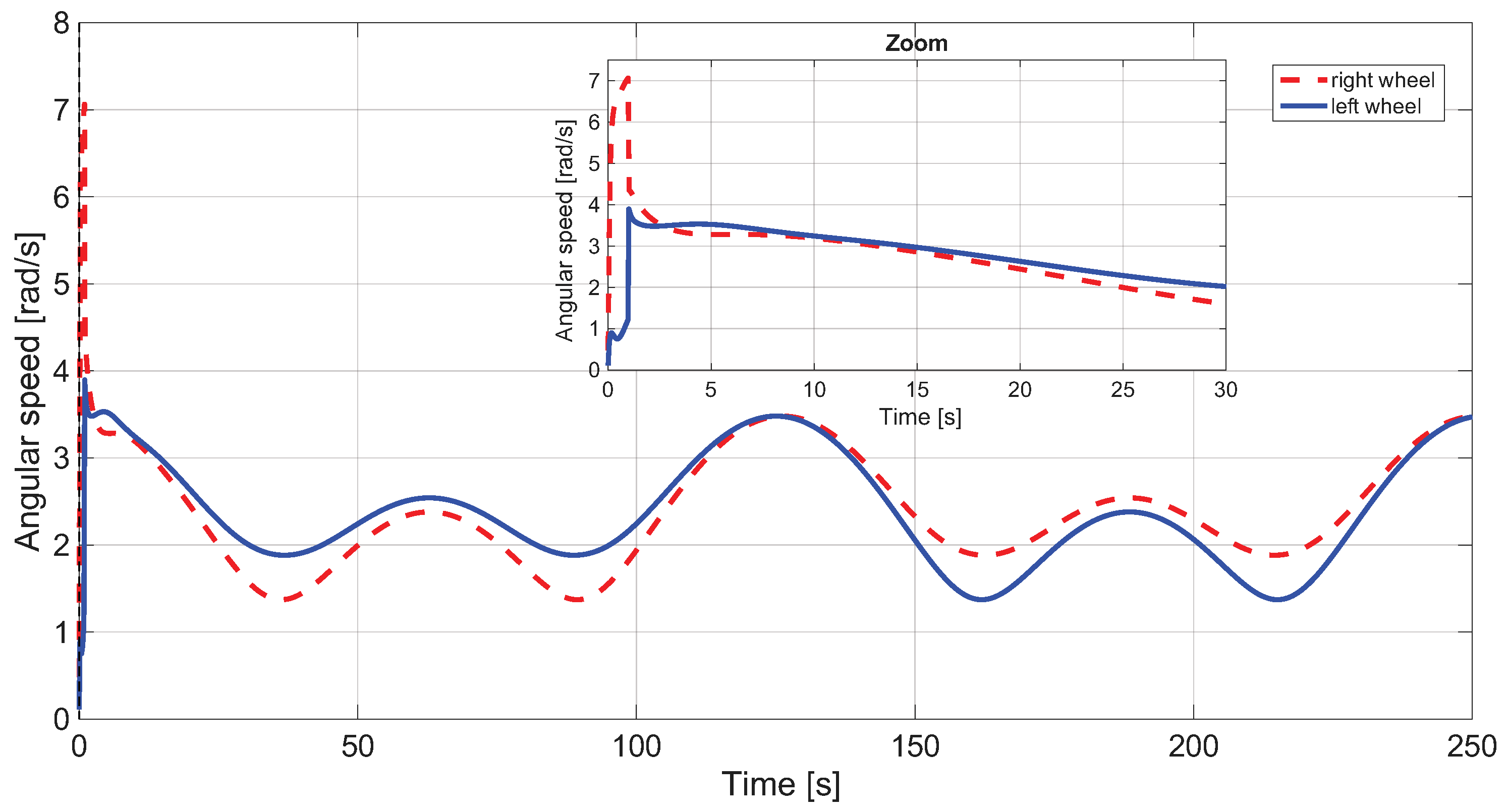
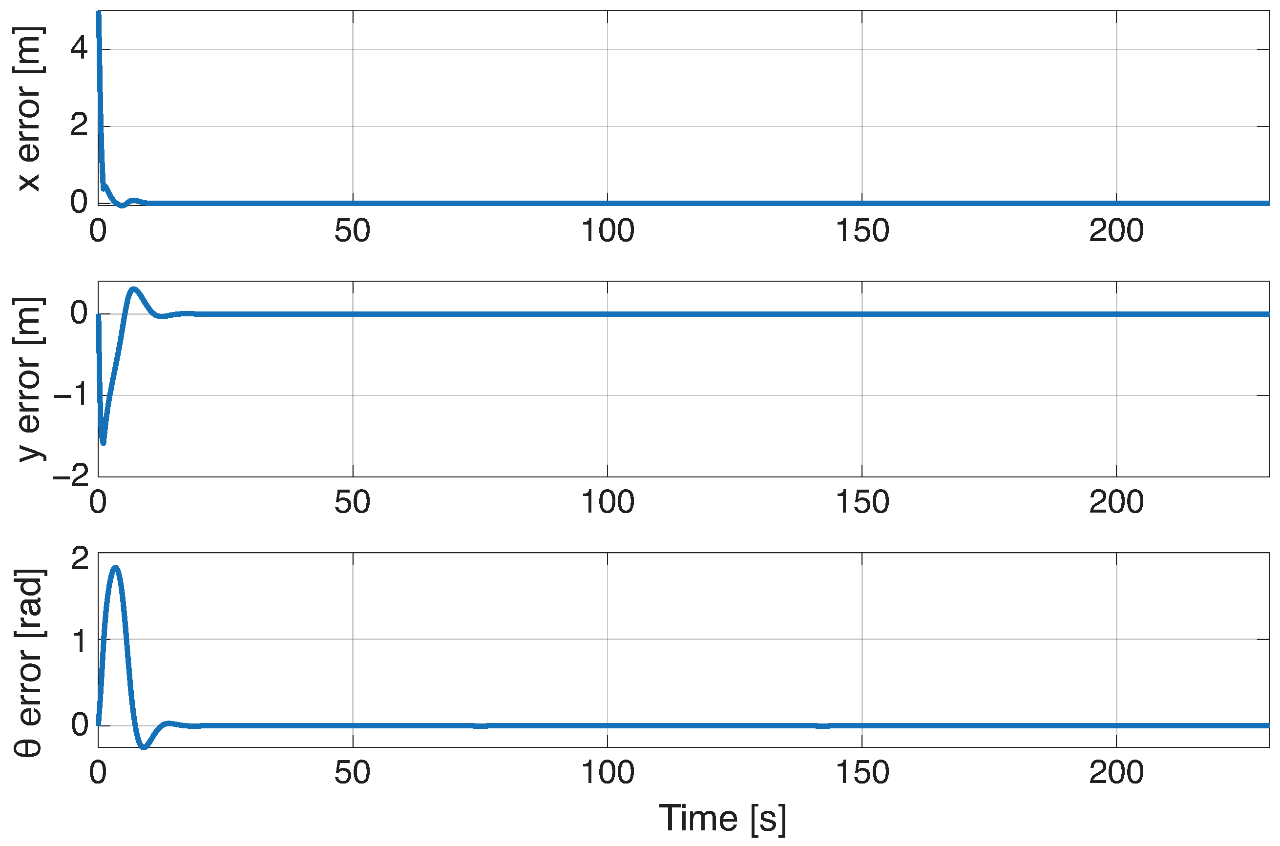
Figure 4 shows the trajectory-tracking response for the circular reference. Since the robot starts away from the desired path, an initial transient is observed. However, the actual trajectory converges to the circular path and remains close to the reference thereafter. This behavior is also reflected in the position-error response shown in Figure 5, where the largest deviations occur at the beginning of the simulation and then decrease rapidly. 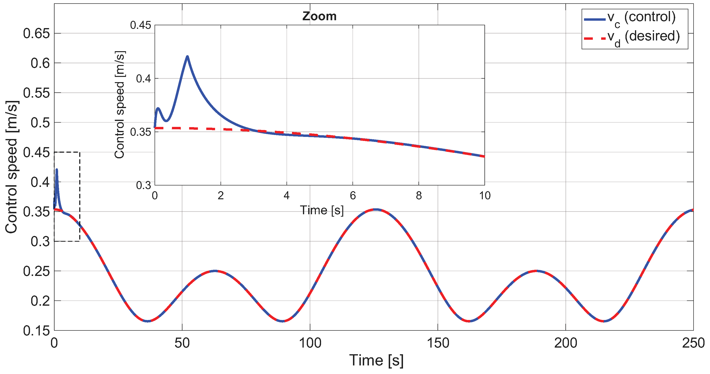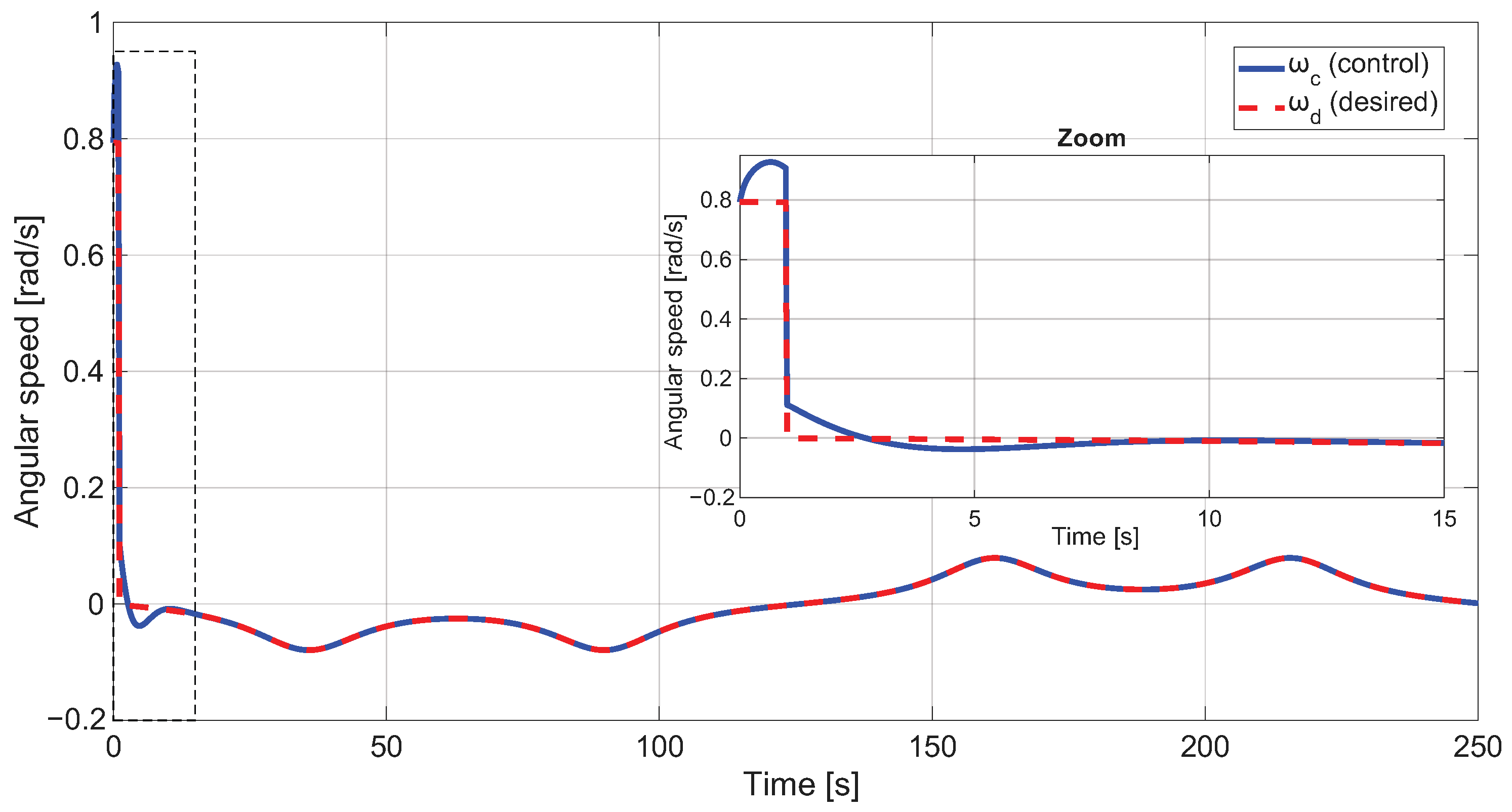The wheel angular velocities in Figure 6 show an initial control effort associated with the convergence phase, followed by a stable steady-state response. Similarly, the commanded linear and angular velocities in Figure 7 and Figure 8 converge to the desired profiles after the initial adjustment.

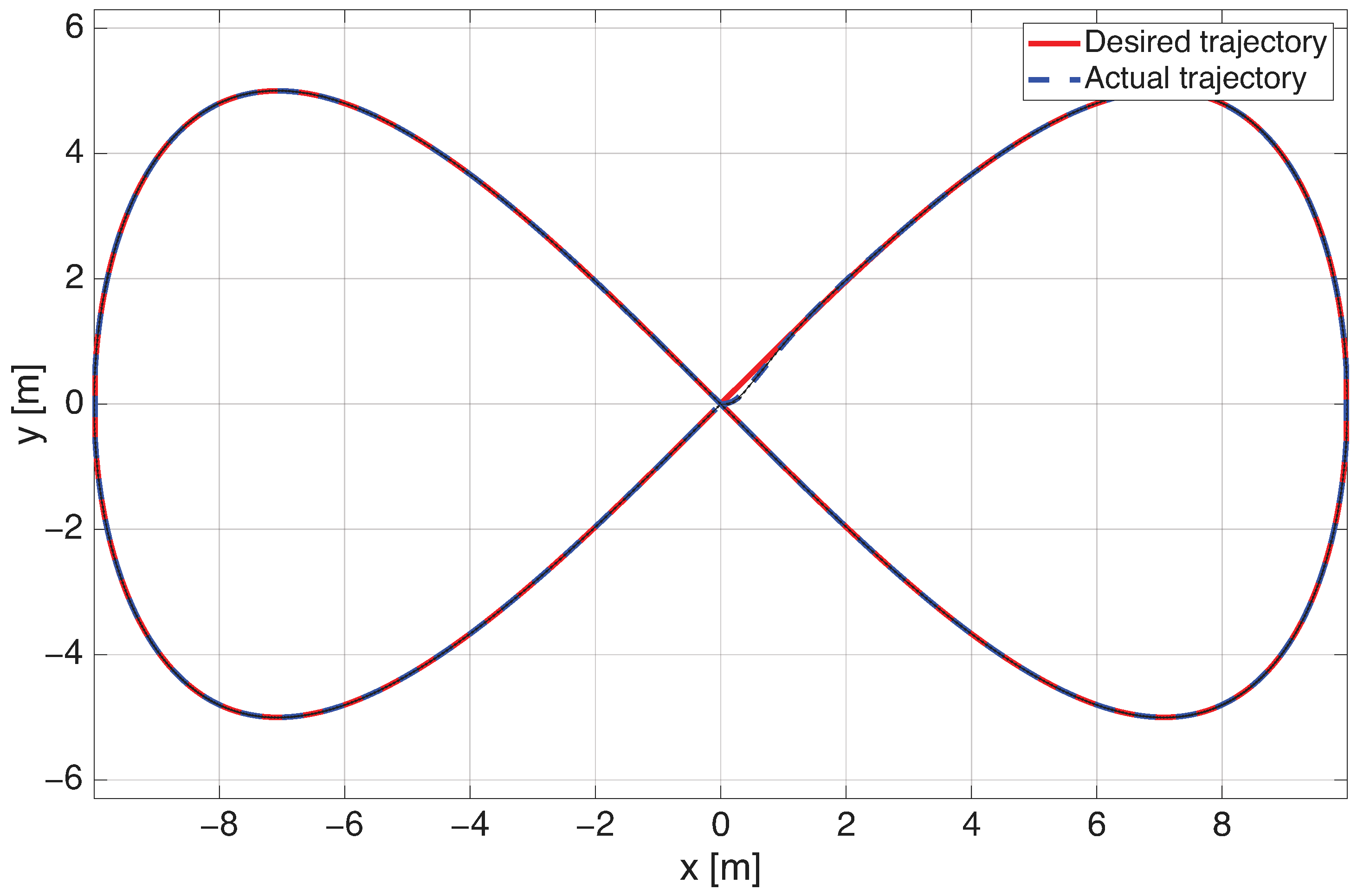
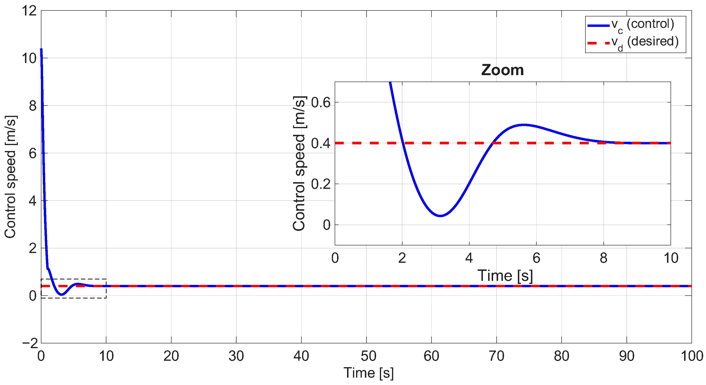
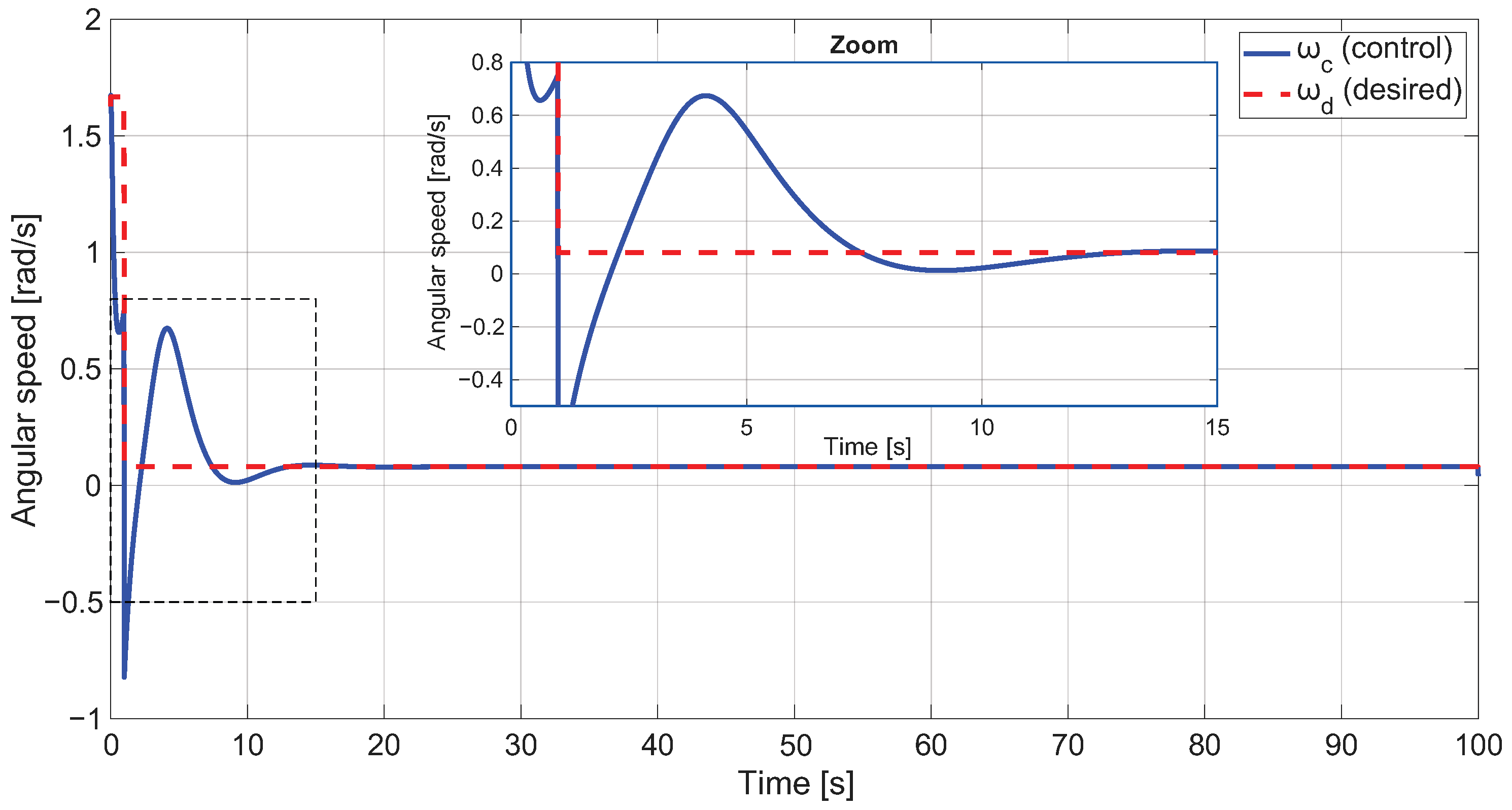
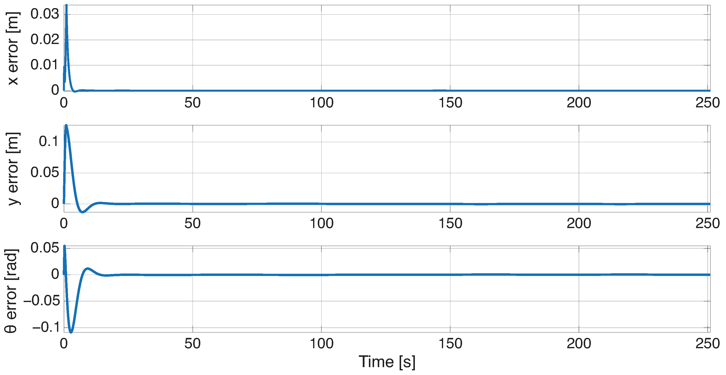
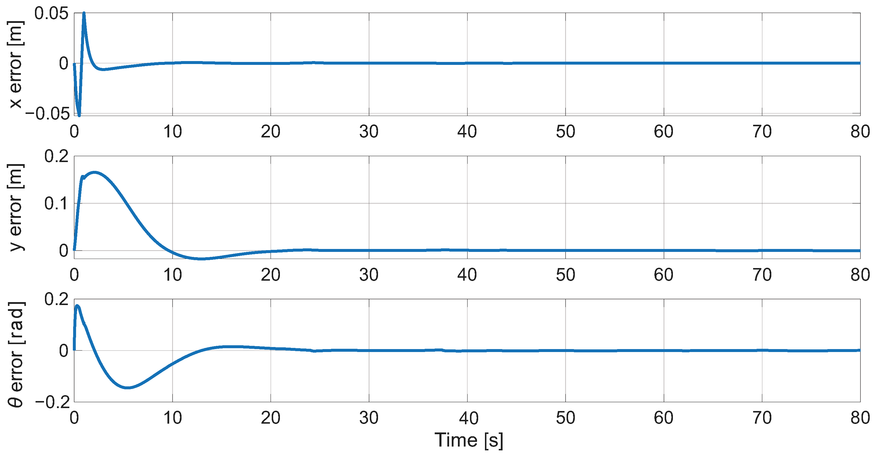
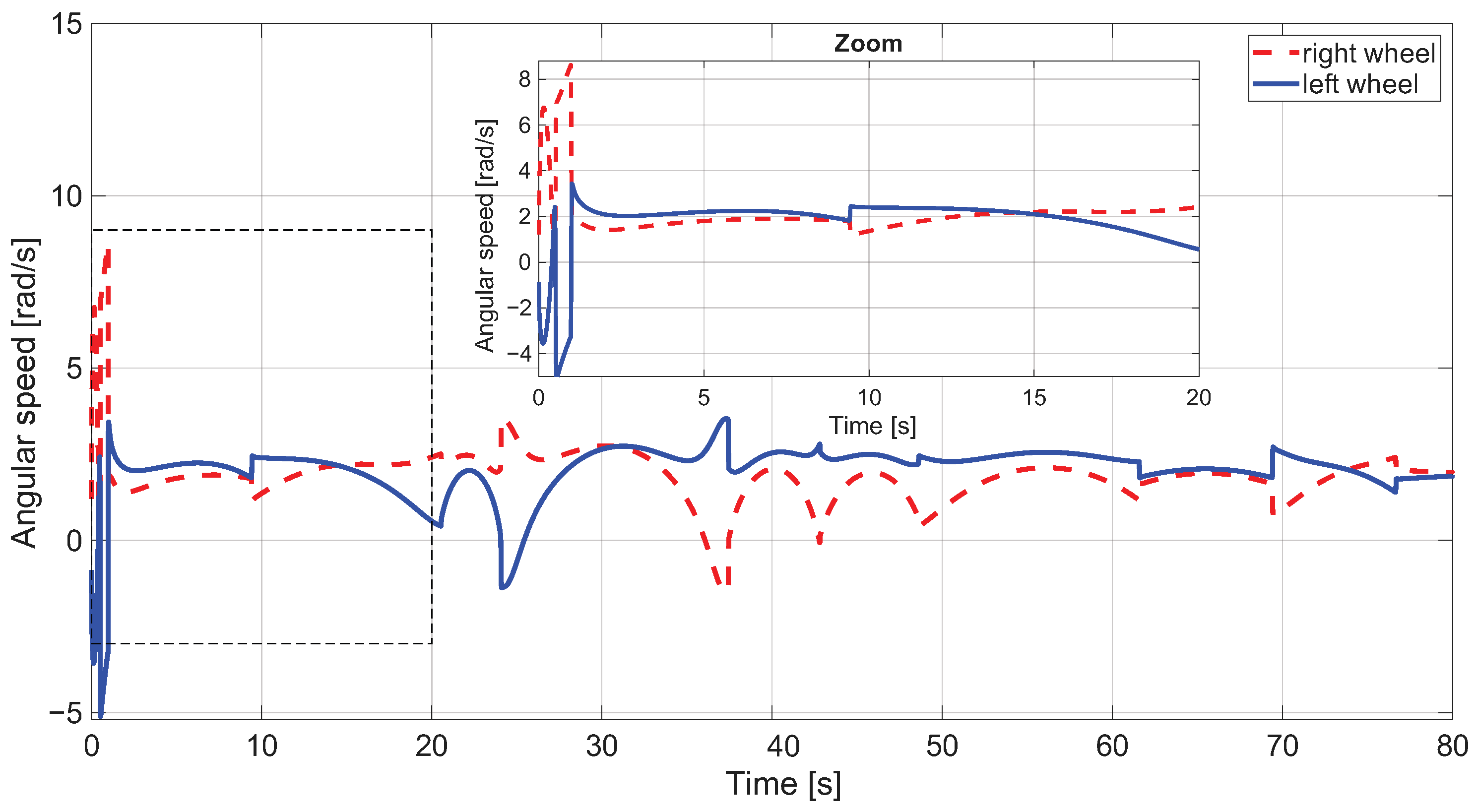
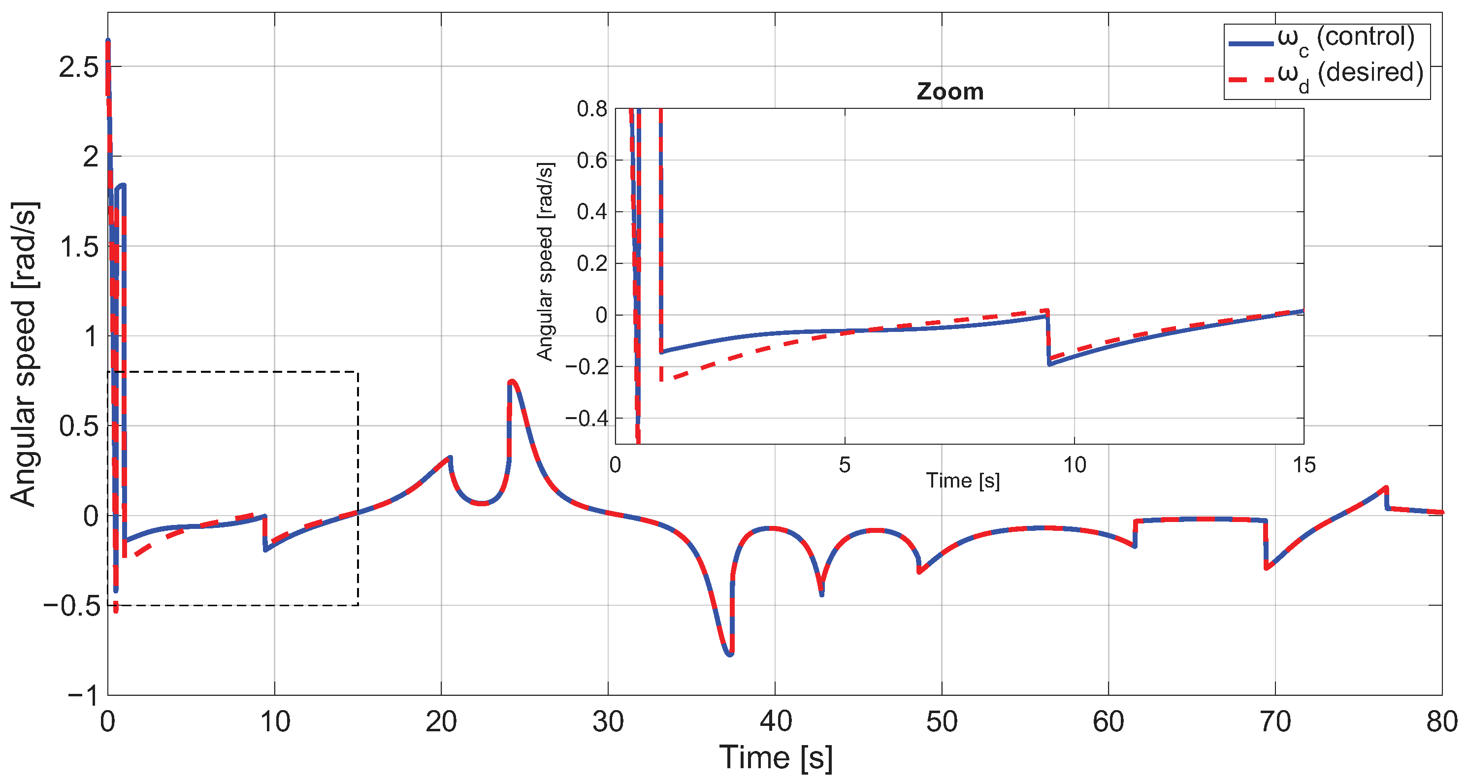
For the lemniscate trajectory, Figure 9 shows that the actual path closely overlaps the desired reference throughout the simulation. Unlike the circular case, the initial pose is closer to the reference path, which reduces the transient mismatch. This is confirmed by the position-error behavior shown in Figure 10, where the tracking errors remain small throughout the simulation. The wheel angular velocities in Figure 11 exhibit a smooth periodic behavior consistent with the curvature changes of the lemniscate. The linear and angular control velocities in Figure 12 and Figure 13 also show bounded responses without abrupt oscillations.

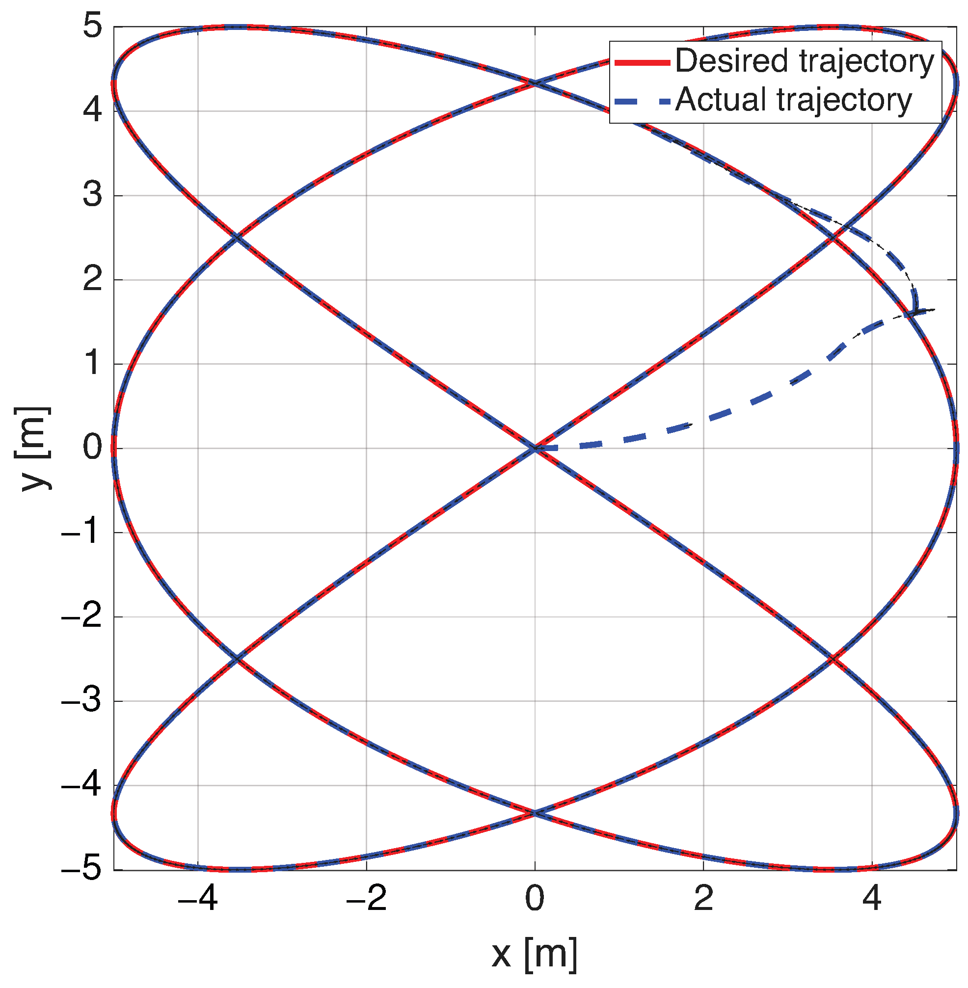
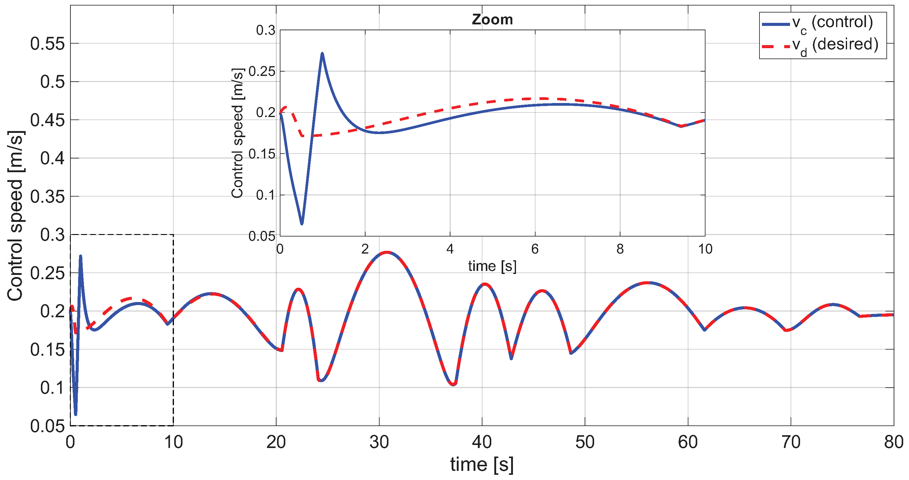
The Lissajous trajectory imposes a more demanding tracking task due to its varying curvature and crossing pattern. As shown in Figure 14, the robot initially approaches the desired curve from a different location, producing a transient error similar to that observed in the circular case. After this initial stage, the actual path follows the reference trajectory with good accuracy. The position errors in Figure 15 decrease rapidly after the initial convergence interval. The wheel angular velocities in Figure 16 remain bounded and vary according to the periodic changes in the path geometry. Figure 17 and Figure 18 show that the control velocities track their desired profiles after the transient stage.

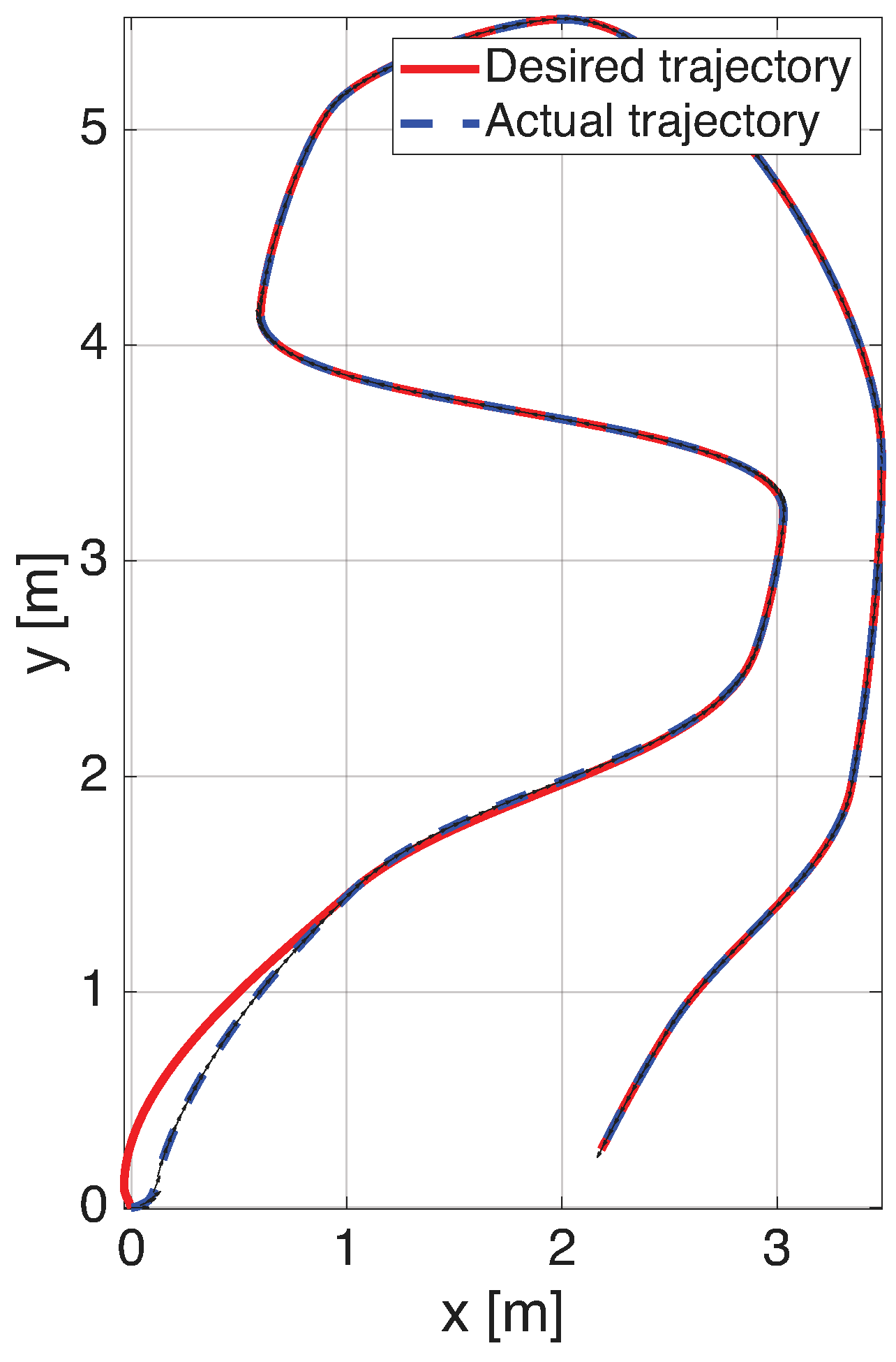
The waypoint-based trajectory represents the most irregular case because the path includes sharper changes in direction. As shown in Figure 19, the actual trajectory follows the general shape of the reference path, although larger local deviations appear near the curved and transition regions. This behavior is expected because waypoint trajectories impose abrupt changes in curvature compared with smooth analytical curves. 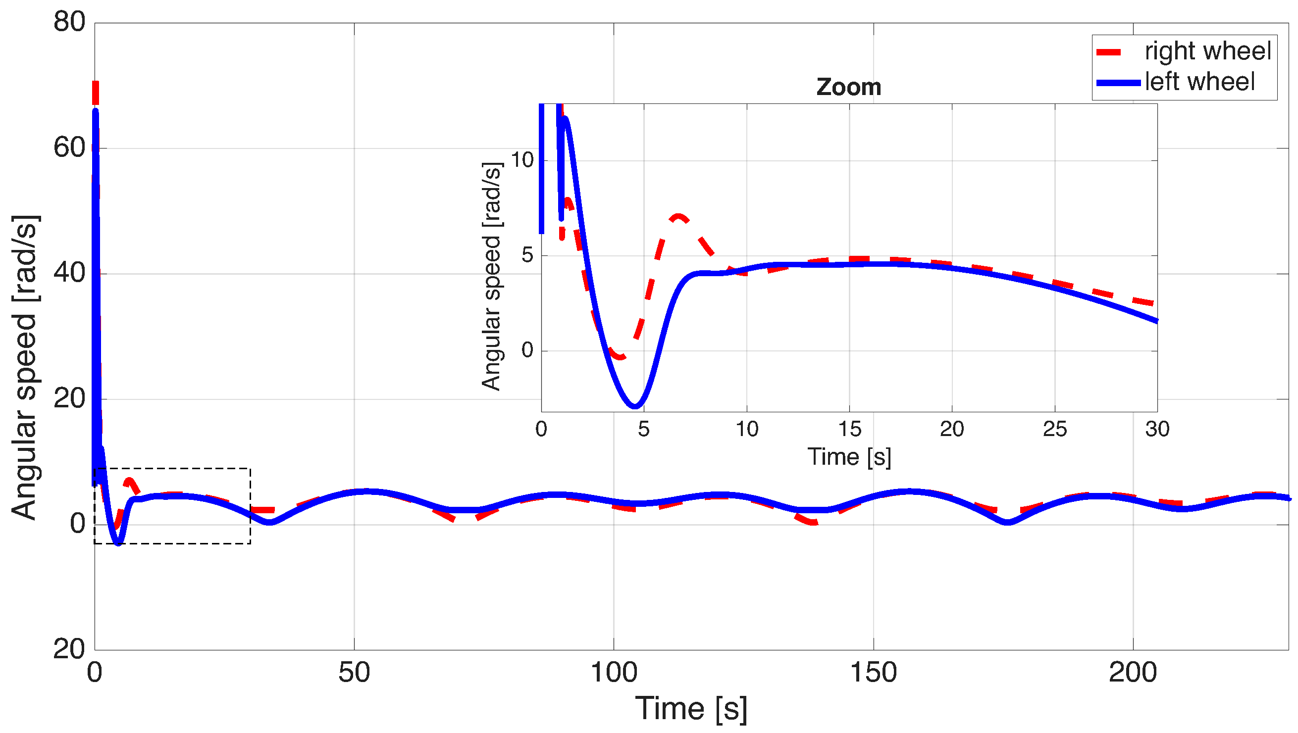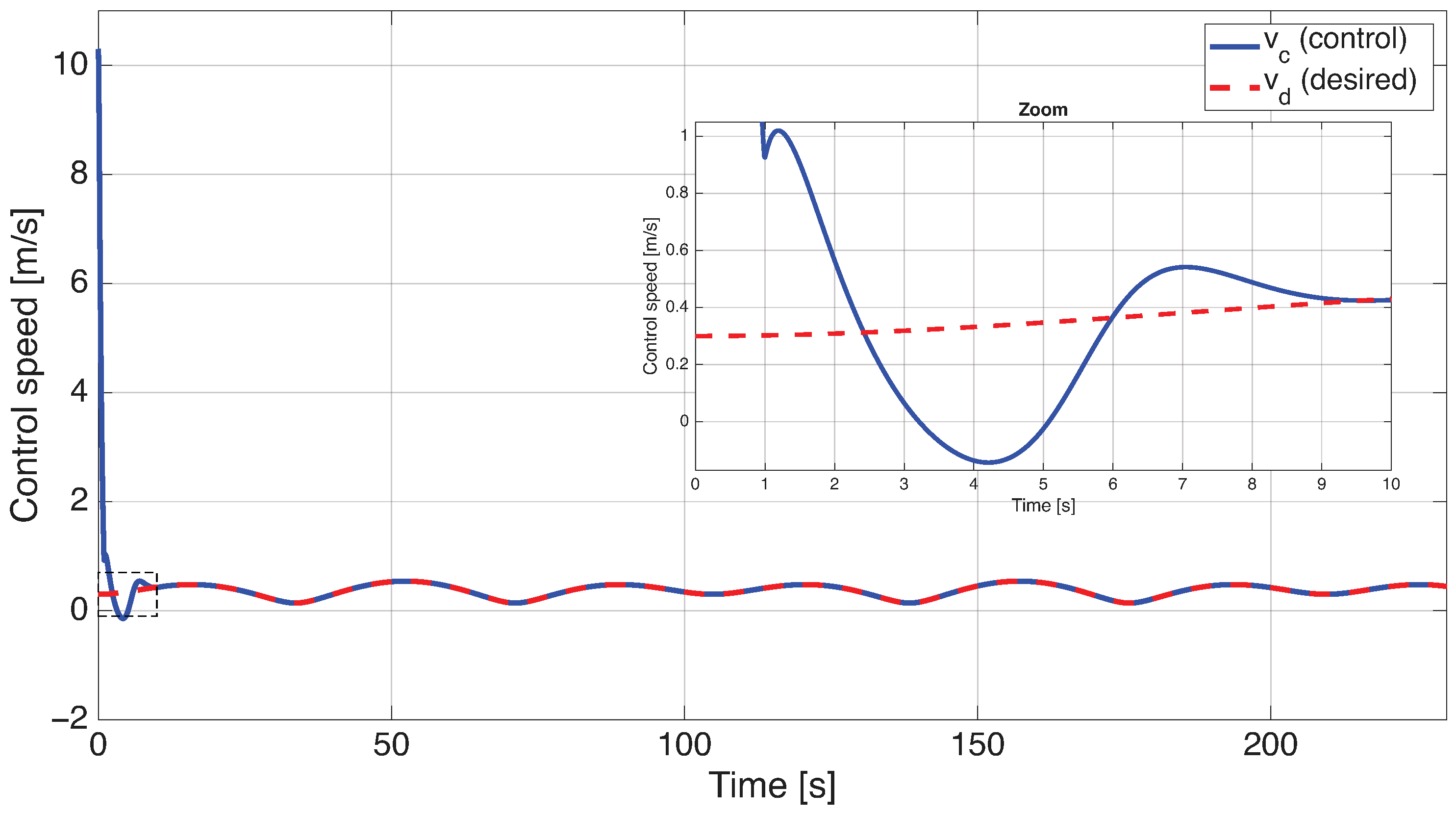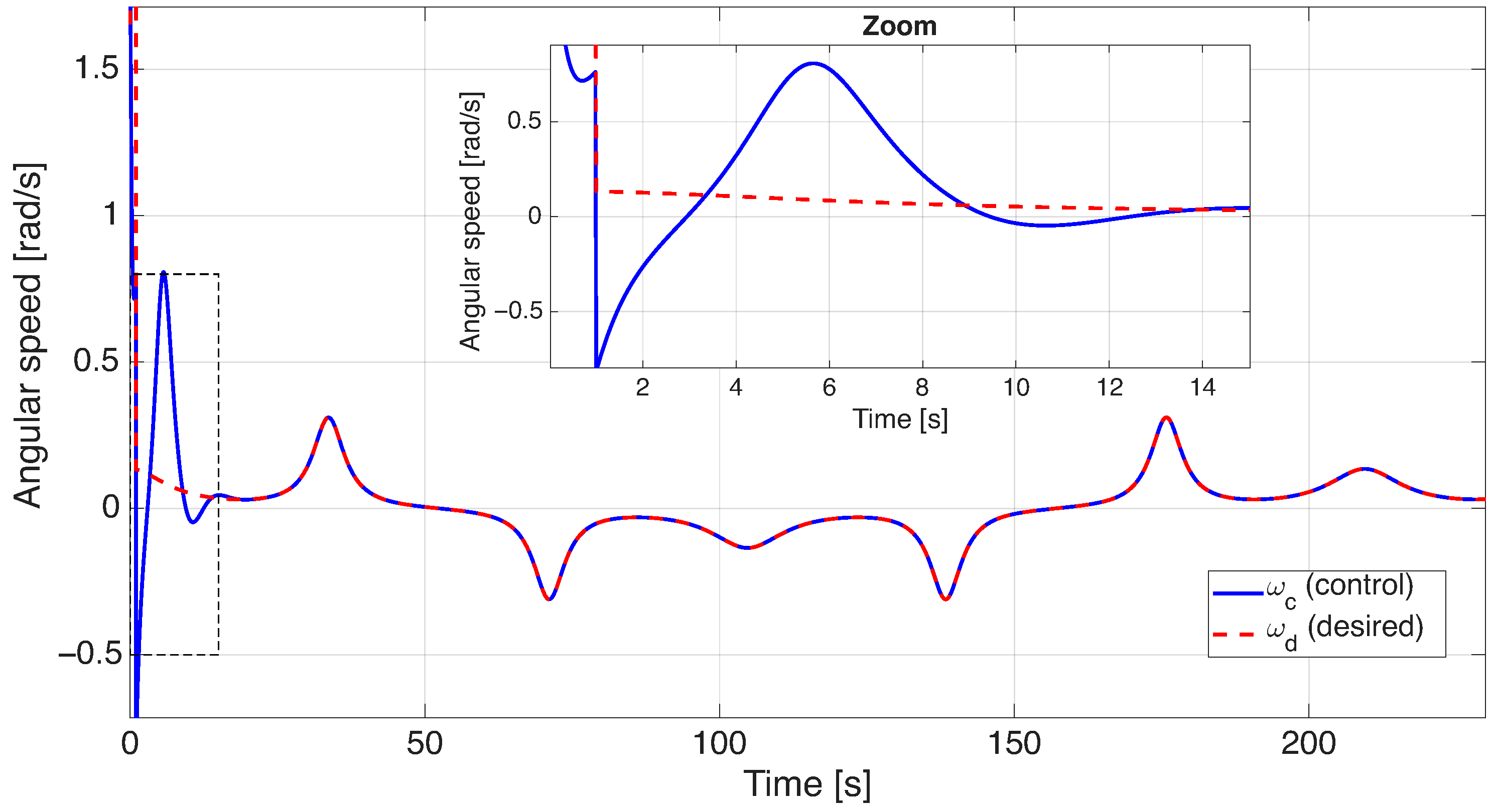The position-error response in Figure 20 confirms that the tracking error remains present during most of the simulation, particularly around the path transitions. Nevertheless, the error remains bounded. The wheel angular velocities shown in Figure 21 present larger variations than in the smooth trajectories, reflecting the higher actuation demand imposed by the waypoint path. The corresponding control velocities in Figure 22 and Figure 23 also show more pronounced changes, especially during the transition segments.

The quantitative performance of the proposed controller is summarized in

Table 3. Summary of tracking performance metrics for the proposed Neural Backstepping controller.

Trajectory	RMSE (x) [m]	RMSE (y) [m]	RMSE ($\mathit{\theta }$) [rad]	RMSE (pos) [m]
Circle	0.009067	0.029495	0.029061	0.030857
Lemniscate	0.001574	0.011263	0.011630	0.011373
Lissajous	0.004878	0.018200	0.017305	0.018842
Waypoints	0.002941	0.036882	0.052374	0.036999

. The lemniscate trajectory produced the lowest position RMSE, with 0.011373 m, which is consistent with its smooth tracking response and favorable initial condition. The Lissajous trajectory achieved a position RMSE of 0.018842 m, whereas the circular trajectory yielded 0.030857 m due to the larger initial convergence phase. The waypoint-based trajectory produced the largest position RMSE, 0.036999 m, which is expected because of the sharper curvature changes and persistent tracking corrections along the path.

Overall, the proposed controller achieved satisfactory tracking performance in all evaluated cases. The position RMSE remained below $0.04$ m for all trajectories, including the waypoint-based path. These results suggest that the adaptive neural component contributes to maintaining accurate tracking under different reference geometries using the same control gains.

Table 4. Trajectory-tracking performance comparison between the conventional Backstepping (BS) controller and the proposed Neural Backstepping (BS-NN) controller for various reference trajectories. The best value for each metric is shown in bold.

Metric RMSE	Unit	Circular		Lemniscate		Lissajous		Waypoints
		BS	BS-NN	BS	BS-NN	BS	BS-NN	BS	BS-NN
$e_x$	m	0.0144	0.0091	0.0034	0.0016	0.0076	0.0045	0.0538	0.0031
$e_y$	m	0.0340	0.0295	0.0134	0.0113	0.0195	0.0167	0.1555	0.0177
$e_{\theta }$	rad	0.0548	0.0291	0.0211	0.0116	0.0338	0.0159	0.7954	0.0582
$e_p$	m	0.0369	0.0309	0.0138	0.0114	0.0210	0.0173	0.1645	0.0180
Improvement	%	16.3		17.4		17.6		89.1

summarizes the trajectory-tracking performance of the conventional Backstepping (BS) controller and the proposed Neural Backstepping (BS-NN) controller for four representative reference trajectories. The evaluated metrics are the root mean square errors (RMSE) in Cartesian coordinates ($e_x$, $e_y$), orientation ($e_{\theta }$), and overall position ($e_p$). The results show that incorporating the adaptive neural network consistently improves tracking for all trajectories: the BS-NN controller yields lower position and orientation errors than the BS controller in every case. The largest gains occur for the waypoint-following trajectory, where position and orientation errors are substantially reduced. This indicates that the adaptive neural compensator effectively mitigates modeling uncertainties and unmodeled nonlinear dynamics, thereby increasing robustness and tracking accuracy.

The last row of Table 4 reports the percentage improvement of BS-NN over BS, based on position RMSE. The BS-NN controller achieves about 16–18% improvement for smooth trajectories and up to 89% for waypoint following, underscoring its effectiveness under demanding conditions. Overall, the BS-NN controller combines the Lyapunov-based stability of Backstepping with the online approximation capability of neural networks, resulting in improved trajectory-tracking performance across varying operating conditions.

4.5. Discussion

The simulation results show that the proposed Neural Backstepping controller can track smooth and waypoint-based trajectories using a single set of control gains. For the circular and Lissajous paths, the main tracking error occurs during the initial convergence phase because the robot starts away from the desired trajectory. After this transient, the actual trajectory closely follows the reference path. For the lemniscate trajectory, the initial condition is more favorable and the tracking error remains small during the complete simulation. For the waypoint-based path, the tracking error is larger and more persistent due to the sharper curvature transitions; nevertheless, the position RMSE remains below $0.04$ m.

The lowest RMSE was obtained for the lemniscate trajectory, whereas the largest RMSE occurred for the waypoint trajectory. This behavior is consistent with the geometric complexity of the references: smooth continuous paths are easier to track, while waypoint-generated paths require stronger velocity corrections and produce larger transient deviations. The wheel angular velocities and control velocity profiles also confirm this trend. Smooth trajectories generate bounded and regular control responses, whereas the waypoint trajectory produces more pronounced variations in the wheel velocities and commanded angular velocity.

These results indicate that the proposed Neural Backstepping controller provides a favorable balance between tracking accuracy and implementation simplicity. The single-hidden-layer neural approximator avoids the computational burden of deeper architectures while providing online adaptation through the output weights. In addition, the same gain configuration was used for all evaluated trajectories, suggesting that the controller can adapt to different reference geometries without trajectory-specific retuning.

5. Conclusions

This paper presented a Neural Backstepping control strategy for trajectory tracking of a differential-drive mobile robot. The proposed approach combines a dynamic-level backstepping controller with a lightweight single-hidden-layer adaptive neural network. The backstepping component provides a Lyapunov-based stabilizing structure, whereas the neural approximator is incorporated to compensate uncertain nonlinear dynamics through online adaptation.

The stability analysis showed that, under bounded neural approximation errors, all closed-loop signals remain bounded and the velocity tracking error is uniformly ultimately bounded. Therefore, the proposed controller guarantees practical stability under the assumptions considered in this work. This result supports the use of the adaptive neural component as a compensation mechanism within the backstepping control structure.

Simulation results were obtained for four reference trajectories: circular, lemniscate, Lissajous, and waypoint-based paths. The proposed controller achieved satisfactory tracking performance in all cases using the same gain configuration and neural network structure. The lowest position RMSE was obtained for the lemniscate trajectory, whereas the waypoint-based trajectory produced the largest error due to its sharper curvature transitions. Nevertheless, the position RMSE remained below $0.04$ m for all evaluated trajectories, indicating accurate tracking performance and stable closed-loop behavior.

The results suggest that the proposed Neural Backstepping controller provides a suitable balance between tracking accuracy, online adaptation capability, and implementation simplicity. In particular, the use of a single-hidden-layer neural approximator avoids the complexity of deeper learning architectures while preserving the ability to compensate persistent tracking deviations. These conclusions are supported by the Lyapunov-based stability analysis and the simulation results presented in this work. However, experimental validation and robustness assessments under external disturbances and parametric uncertainties remain topics for future investigation.

The main limitation of this work is that the validation was restricted to numerical simulations. Future work will focus on the experimental implementation of the proposed controller on a real differential-drive mobile robot platform. In addition, further studies will investigate explicit robustness evaluations under parametric uncertainties, external disturbances, and actuator limitations, as well as comparative assessments against conventional backstepping and other nonlinear control strategies. These extensions will complement the theoretical developments presented in this work and provide additional insights into the practical performance of the proposed Neural Backstepping framework.