Identification, Evolution, and Temporal Classification of Operational States at Major Japanese Airports

Abstract

To address the limitations of existing approaches that rely primarily on individual operational indicators and provide limited insight into the dynamic evolution of airport operational states, this study develops a two-stage analytical framework integrating unsupervised state identification and supervised temporal classification. Using monthly operational data from seven major Japanese airports between January 2010 and March 2024, the proposed framework first applies K-means clustering to identify latent operational states based on multidimensional indicators reflecting growth dynamics, operational efficiency, and relative operational level. Three distinct states are identified: a low-activity state, a recovery state, and a rapid-rebound state. Here, the rapid-rebound state denotes a temporary operational regime characterized by exceptionally strong year-on-year growth from a comparatively depressed base, rather than the highest absolute utilization rates or 2019-relative operational level. The results reveal clear stage-specific characteristics and transition patterns, with the recovery state serving as the most persistent and relatively stable operational regime, while rapid-rebound episodes are less frequent, less stable, and often transition back to the recovery state. The supervised component subsequently evaluates whether recovery and rapid-rebound labels retrospectively identified through full-sample clustering can be distinguished using lagged operational characteristics. Six classification algorithms, including logistic regression, radial basis function support vector machine (RBF-SVM), random forest, gradient boosting, XGBoost, and LightGBM, are compared using a chronologically ordered 60/20/20 partition applied only at the supervised-classifier stage, with SMOTE applied exclusively to the training subset. Because the standardization parameters, K-means solution, and target state labels were derived from the complete 2010–2024 sample, and because several 2019-relative variables were constructed using an ex post benchmark, the reported results represent classifier-stage temporal evaluation of retrospectively identified full-sample labels rather than end-to-end out-of-sample validation or prospective real-time prediction. Under the prespecified common SMOTE-based six-model comparison, LightGBM yields the highest point estimates for macro-F1 and rapid-rebound-state recall, reaching 0.6864 and 0.5588, respectively. Given that the training subset contains only seven rapid-rebound observations, these estimates should be interpreted cautiously. An exploratory sensitivity analysis using alternative imbalance-handling strategies produces materially different point estimates, indicating that minority-state classification performance is sensitive to the selected imbalance treatment. The SHAP-based feature attribution results indicate that short-term lagged growth indicators and twelve-month 2019-relative operational-level variables contribute strongly to the fitted distinction between the recovery and rapid-rebound state labels. Although the supervised analysis is restricted to distinguishing the recovery and rapid-rebound state labels, the proposed framework provides a multidimensional approach for airport state identification, temporal evolution analysis, retrospective operational monitoring, and post-shock recovery assessment. A genuinely prospective application would require reconstructing all input variables using information available at each forecast origin and re-estimating the models accordingly.

1. Introduction

Airports are core nodes in regional transport networks and air transportation systems. Their operational performance reflects fluctuations in air transport demand and changes in airport resource allocation, flight organization, and transport efficiency [1,2]. With the continued evolution of the global air transportation network, airport operations have exhibited significant dynamism, stage specificity, and heterogeneity. In particular, under external shocks, passenger throughput, flight operations, and cargo volume often fluctuate simultaneously; however, substantial differences exist among airports in terms of the pace of change, recovery paths, and stage characteristics [3,4,5,6]. Compared with a static description of airport business scale, identifying stage differences, transition paths, and evolutionary patterns in airport operational states across different periods is more conducive to understanding the underlying organizational logic and recovery mechanisms of airport operation systems while also providing systematic evidence for retrospective operational evaluation, stage comparison, and recovery assessment. Therefore, accurately identifying airport operational states from multidimensional indicators, revealing their dynamic evolution patterns, and examining their temporal separability have become important issues in airport operation research.

Japan’s airport system, characterized by a clear network hierarchy, diverse airport types, and complex operational scenarios, provides a suitable context for examining the identification, evolution, and temporal classification of airport operational states. According to information published by Japan’s Ministry of Land, Infrastructure, Transport and Tourism, Japan’s airport system includes core airports such as Haneda, Narita, and Kansai, which serve as international gateways and national hubs [7,8,9], as well as important nodes such as New Chitose, Fukuoka, and Naha, which function as regional connectors and tourism gateways [10,11]. Differences among these airports in hinterland coverage, passenger–cargo structure, and operational rhythm provide a sound basis for comparing stage differentiation and heterogeneous evolution in airport operational states. At the same time, the Japanese government has continuously released relatively standardized aviation and tourism statistics, providing reliable support for characterizing airport operational states from multiple dimensions, including passenger traffic, flight movements, cargo throughput, capacity, and relative operational level. Moreover, while Japan’s air transportation system has operated relatively steadily over the long term, it has also experienced substantial fluctuations and recovery under external shocks, making it easier to identify and test the persistence, transition, and restructuring of airport states over an extended period. On this basis, this study focuses on seven major Japanese airports—Tokyo Haneda, Narita, Kansai, Osaka (Itami), New Chitose, Fukuoka, and Naha—as empirical cases.

Existing studies have mainly focused on the analysis of changes in single indicators such as passenger throughput, flight volume, and cargo volume [12,13,14,15,16], or have examined airport operations from the perspectives of demand forecasting, pandemic impact assessment, and route recovery [17,18,19,20,21,22]. Although these studies provide an important foundation for understanding fluctuations in airport operations, they suffer from two major limitations. First, some studies [12,13,17,20] rely on single-scale-related indicators and fail to conduct a comprehensive analysis from multiple dimensions such as growth dynamics, operational efficiency, and relative operational level, making it difficult to identify stage-specific operational states across different periods. Second, most existing studies focus on describing quantitative changes and conducting short-term forecasting [23,24,25,26,27] while paying relatively limited attention to the evolution paths and transition structures of airport operational states and to whether retrospectively identified operational regimes can be distinguished using temporally lagged multidimensional characteristics [28,29,30]. Airport operational-state evolution may involve complex temporal dependencies and interactions shaped by operational inertia and external shocks. Whether these relationships exhibit meaningful nonlinearity is therefore examined empirically in the subsequent model comparison rather than assumed a priori.

To address these issues, this study develops an analytical framework integrating unsupervised learning for latent state identification and supervised learning for retrospective temporal classification. Specifically, K-means clustering [31] is first employed to identify heterogeneous airport operational states from multidimensional operational characteristics. Six classification algorithms are then systematically tuned and compared to examine whether the retrospectively defined recovery and rapid-rebound states can be distinguished using temporally lagged operational features. Related research in maritime transportation has demonstrated that comparative machine learning prediction and classification, combined with feature-importance and SHAP analyses, can support operational decision-making in complex port environments [32]. Unlike studies that predict vessel stay or delay outcomes, the present study focuses on the retrospective identification, evolution, and temporal separability of multidimensional airport operational states. Using seven major Japanese airports—Tokyo Haneda, Narita, Kansai, Osaka (Itami), New Chitose, Fukuoka, and Naha—as empirical cases, monthly operational data from January 2010 to March 2024 are analyzed to investigate airport-state identification, temporal evolution, and classification. This study contributes by shifting airport operational analysis from static indicator-based evaluation toward a state-based perspective, revealing the temporal persistence and transition structures of different operational states, and systematically comparing the ability of different machine learning approaches to distinguish ex post-defined state labels in chronologically later observations.

2. Method

2.1. Establishment of the Airport Operational State Identification Model

Airport Operational State Identification Model

• Model Development Logic and Structure

Airport operational state is treated as a latent construct jointly reflected by growth dynamics, operational efficiency, and relative operational level. Accordingly, each airport-month observation is represented by multidimensional operational indicators, and unsupervised learning is used to identify latent groupings within the resulting feature space. The identified clusters are subsequently interpreted according to their centroid profiles and assigned substantive operational-state labels. The framework therefore comprises four linked elements: airport-month sample representation, feature construction, latent-state identification, and result interpretation.

• Airport State Identification Method Based on K-means Clustering

This study employs the K-means clustering method [31] to group airport-month observations with similar multidimensional operational characteristics. The clustering procedure consists of four steps:

• Eight indicators reflecting growth dynamics, operational efficiency, and relative operational level are used to represent each airport-month observation.
• All indicators are standardized using z-scores to ensure comparability and prevent variables with larger numerical ranges from dominating the distance calculation.
• Candidate solutions with K = 2 to K = 8 are evaluated using the elbow criterion, average silhouette score, Calinski–Harabasz index, Davies–Bouldin index, and substantive interpretability. The final value of K is selected through joint consideration of these criteria rather than predetermined a priori.
• For each candidate solution, observations are assigned to their nearest centroids, and the centroids are iteratively updated until convergence. The final clusters are interpreted according to their centroid profiles and labelled as low-activity, recovery, and rapid-rebound states.

• Implementation of the Airport Operational State Identification Model

• Establishment of the Feature Indicator System

To identify latent airport operational states from multidimensional operational characteristics, this study constructs a feature indicator set comprising variables closely related to airport development and operating conditions. The selected indicators capture three complementary dimensions—growth dynamics, operational efficiency, and relative operational level—as shown in

Table 1. Feature Indicator Set for the Airport Operational State Identification Model.

Indicator	Category	Dimension Reflected	Implication of a High Value	Implication of a Low Value
Year-on-year passenger growth	Growth dynamics	Growth rate of passenger traffic	Rapid growth	Decline or slow growth
Year-on-year flight growth	Growth dynamics	Growth rate of flight volume	Rapid growth	Decline or slow growth
Year-on-year cargo growth	Growth dynamics	Growth rate of cargo volume	Rapid growth	Decline or slow growth
Seat utilization rate	Operational efficiency	Degree of seat utilization	High efficiency	Low efficiency
Weight utilization rate	Operational efficiency	Degree of cargo capacity utilization	High efficiency	Low efficiency
2019-relative passenger level	Relative operational level	Passenger activity relative to the corresponding 2019 level	Close to or above the corresponding 2019 level	Substantially below the corresponding 2019 level
2019-relative flight level	Relative operational level	Flight activity relative to the corresponding 2019 level	Close to or above the corresponding 2019 level	Substantially below the corresponding 2019 level
2019-relative cargo level	Relative operational level	Cargo activity relative to the corresponding 2019 level	Close to or above the corresponding 2019 level	Substantially below the corresponding 2019 level

. The substantive labels of the resulting clusters, namely, the low-activity state, recovery state, and rapid-rebound state, are assigned only after the K-means clustering results and the corresponding cluster-centroid profiles are examined.

The calculation methods are as follows:

Year-on-year passenger growth $R_P$:

$$R_P={\displaystyle \frac{P_{cur}{P}_{last}}{P_{last}}}\times 100\%$$

(1)

Year-on-year flight growth $R_F$:

$$R_F={\displaystyle \frac{F_{cur}{F}_{last}}{F_{last}}}\times 100\%$$

(2)

Year-on-year cargo growth $R_G$:

$$R_G={\displaystyle \frac{G_{cur}{G}_{last}}{G_{last}}}\times 100\%$$

(3)

Seat utilization rate $U_S$:

$$U_S={\displaystyle \frac{P_{cur}}{S}}$$

(4)

Weight utilization rate $U_T$:

$$U_T={\displaystyle \frac{G_{cur}}{T}}$$

(5)

2019-relative passenger level $L_{p,2019}$:

$$L_{P,2019}={\displaystyle \frac{P_{cur}}{P_{19avg}}}\times 100\%$$

(6)

2019-relative flight level $L_{F,2019}$:

$$L_{F,2019}={\displaystyle \frac{F_{cur}}{F_{19avg}}}\times 100\%$$

(7)

2019-relative cargo level $L_{G,2019}$:

$$L_{G,2019}={\displaystyle \frac{G_{cur}}{G_{19avg}}}\times 100\%$$

(8)

where $P_{cur}$ is the passenger volume in the current month; $P_{last}$ is the passenger volume in the same month of the previous year; $P_{19avg}$ is the average passenger volume in the corresponding month of 2019; $F_{cur}$ is the number of flights in the current month; $F_{last}$ is the number of flights in the same month of the previous year; $F_{19avg}$ is the average number of flights in the corresponding month of 2019; $G_{cur}$ is the cargo weight in the current month; $G_{last}$ is the cargo weight in the same month of the previous year; $G_{19avg}$ is the average cargo weight in the corresponding month of 2019; $S_S$ is the number of available seats; and $T$ is the number of available ton-kilometers.

The year 2019 was selected as a common ex post reference because it was the last complete calendar year preceding the large-scale disruption caused by the COVID-19 pandemic. The resulting ratios provide a consistent retrospective benchmark across the 2010–2024 sample. For pre-2019 observations, however, the 2019 benchmark was not contemporaneously available; these ratios should therefore be interpreted as ex post normalized operational-level measures. Accordingly, the term “recovery” is most directly applicable to the post-2019 period. Because these variables and their lagged values are included in the supervised analysis, the classification task is retrospective rather than prospective. A real-time application would require forecast-origin-specific baselines and complete model re-estimation.

2.

Data Standardization

Because the subsequent analysis applies K-means clustering to a multidimensional set of airport operational indicators, data standardization is performed before clustering. Since K-means relies on Euclidean distance as its core similarity measure, differences in measurement units and numerical scales may cause variables with larger magnitudes to disproportionately influence the estimation of distances and cluster centroids. To address this issue, z-score standardization is applied to each feature. Specifically, standardization is performed globally across the pooled set of all airport-month observations from the seven airports over the entire study period, rather than separately within individual airports or time periods. Thus, for each feature j, the sample mean $\overline{x_j}$ and standard deviation $s_j$ are calculated using all available airport-month observations. This pooled standardization strategy preserves meaningful differences across airports and time periods while placing all features on a common scale, thereby supporting the identification of common operational states across the full sample. Importantly, the pooled standardization parameters, the selection of K, and the final K-means cluster centroids were all estimated using the complete 2010–2024 sample. Accordingly, the resulting operational-state labels should be understood as retrospective full-sample constructs. The subsequent 60/20/20 chronological partition was not applied to this upstream state-identification stage. Therefore, observations belonging to the later validation and test periods contributed to the retrospective definition of the target state labels used in the supervised classification analysis.

$$z_{ij}={\displaystyle \frac{x_{ij}-\overline{x_j}}{s_j}}$$

(9)

where $\overline{x_j}$ and $s_j$ denote, respectively, the mean and standard deviation of the j-th indicator calculated across all pooled airport-month observations in the full clustering sample.

3.

Implementation of the Clustering Model

Let $n$ denote the number of airport-month observations and $m$ the number of variables. Let $z_{ij}$ represent the standardized value of the j-th indicator for the i-th sample. After standardization, the indicator values of all samples can be expressed in matrix form as follows:

$$Z=\begin{array}{cccc}{z}_{11}& z_{12}& \dots & z_{1m}\\ z_{21}& z_{22}& \dots & z_{2m}\\ ⋮& ⋮& \ddots & ⋮\\ z_{n1}& z_{n2}& \dots & z_{nm}\end{array}$$

(10)

This study uses Euclidean distance to measure the similarity between samples:

$$d_{ij}=\sqrt{{\displaystyle {\sum }_{r=1}^m(z_{ir}-z_{jr}{)}^2}}$$

(11)

where $d_{ij}$ denotes the Euclidean distance between samples i and j, m denotes the number of indicators, and r indexes the indicators in the standardized feature space.

4.

Interpretation of Clustering Results

Based on the K-means clustering results, the three clusters are, respectively, interpreted as the low-activity state, recovery state, and rapid-rebound state according to their joint centroid patterns in terms of growth dynamics, utilization rates, and 2019-relative operational levels, as shown in

Table 2. Typical Features of the Three Airport Operational States.

State	Growth Dynamics	Operational Efficiency	Relative Operational Level
Low-activity state	Negative or weak growth	Low	Substantially below the 2019 level
Recovery state	Moderate positive growth	High	Close to or above the 2019 level
Rapid-rebound state	Exceptionally strong year-on-year growth	Medium	Below the 2019 level

. In this classification, the term “rapid-rebound state” refers to an operational regime characterized by exceptionally strong year-on-year growth from a comparatively depressed base; it does not indicate that utilization rates or 2019-relative operational levels are the highest among the three states. The recovery state, by contrast, exhibits higher utilization rates and operational levels closer to the 2019 benchmark and therefore represents a more stable and near-normal operating regime.

2.2. Airport Operational State Evolution and Temporal Classification Model

2.2.1. Principles of Temporal State Classification

Airport operational states may exhibit temporal dependence because growth dynamics, resource utilization, and relative operational level are affected by short-term operational inertia, stage continuity, and seasonality. The identified transition patterns also indicate persistence and path dependence, particularly the relative stability of the recovery state and the tendency of the low-activity and rapid-rebound states to transition through the recovery state. The three states should therefore not be interpreted as a simple ordinal sequence.

On this basis, the supervised component examines whether retrospectively defined operational-state labels can be distinguished using one-, three-, and twelve-month lagged operational characteristics. Because the labels were derived from full-sample clustering and several variables use an ex post 2019 benchmark, the analysis evaluates temporal separability within a retrospectively constructed dataset rather than prospective real-time forecasting performance.

2.2.2. Development of the Retrospective Temporal Classification Model

The framework contains two related but methodologically distinct components. The state-identification and transition-analysis component retains all three operational states and characterizes their monthly occurrence, persistence, and movement. The supervised component is restricted to the recovery and rapid-rebound states because low-activity observations are temporally concentrated around the external-shock period and are too sparse in the chronological training window to support reliable held-out classification.

Because the target labels were generated using pooled standardization and K-means clustering fitted to the complete 2010–2024 sample, observations in the later validation and test periods contributed to label construction but not to supervised-model fitting, SMOTE processing, or hyperparameter selection. The experiment therefore assesses whether lagged operational profiles reproduce retrospectively identified labels in chronologically later observations; it is not an end-to-end out-of-sample evaluation, a prospective forecasting exercise, or a deployable real-time early-warning system.

2.2.3. Rationale for Selecting Binary Classification Rather than Anomaly Detection

Anomaly detection is most appropriate when unlabeled observations are assessed against a predefined normal operating regime. In the present study, however, K-means provides explicit retrospective state labels, and the supervised objective is to distinguish two substantively defined and partially overlapping operational states. The rapid-rebound state is a recurring regime characterized by exceptionally strong growth from a comparatively depressed base, rather than an erroneous or isolated outlier. Binary classification was therefore adopted so that the identified labels could be used directly and evaluated through class-specific precision, recall, F1-score, and confusion matrices.

Anomaly detection nevertheless remains a useful direction for prospective operational monitoring. Such an application would require an independently defined normal reference period, an anomaly-score threshold, and a genuinely prospective validation design.

2.2.4. Feature Construction and Variable Description

• Dependent Variable Definition

Under this conditional supervised classification setting, the distinction between the retrospectively defined recovery and rapid-rebound states was formulated as a binary classification problem. For airport i in month t, the dependent variable was defined as follows:

$$Y=\left\{\begin{array}{ll}0,& \mathrm{if\; the\; airport\; is\; in\; the\; recovery\; state}\\ 1,& \mathrm{if\; the\; airport\; is\; in\; the\; rapid-rebound\; state}\end{array}\right.$$

(12)

Accordingly, the rapid-rebound state was treated as the positive class, whereas the recovery state was treated as the negative class throughout model training, validation, and evaluation.

2.

Feature Construction

Drawing on the eight core indicators used in the K-means clustering procedure—year-on-year passenger growth, year-on-year flight growth, year-on-year cargo growth, seat utilization rate, weight utilization rate, 2019-relative passenger level, 2019-relative flight level, and 2019-relative cargo level—this study constructs three lagged features for each indicator: a one-month lag, a three-month lag, and a twelve-month lag corresponding to the same month of the previous year.

Specifically, the one-month lag denotes the value of an indicator in the immediately preceding month, the three-month lag denotes its value three months earlier, and the twelve-month lag denotes its value in the corresponding month of the previous year. These lagged variables are included to represent short-term continuity, quarterly scale adjustment, and annual seasonality in airport operations. Annual seasonal characteristics were represented through the twelve-month lagged variables corresponding to the same calendar month of the previous year. No additional month variable was included as an independent predictor in the supervised classification models. The final supervised feature set therefore consisted of 24 lagged variables derived from the eight operational indicators at one-month, three-month, and twelve-month lags, as presented in

Table 3. Features Used in the Retrospective Temporal State Classification Model.

Feature Name	Symbol
One-month lag of year-on-year passenger growth	$R_{Plag1}$
One-month lag of year-on-year flight growth	$R_{Flag1}$
One-month lag of year-on-year cargo growth	$R_{Glag1}$
One-month lag of seat utilization rate	$U_{Slag1}$
One-month lag of weight utilization rate	$U_{Tlag1}$
One-month lag of 2019-relative passenger level	$L_{P,2019}^{lag1}$
One-month lag of 2019-relative flight level	$L_{F,2019}^{lag1}$
One-month lag of 2019-relative cargo level	$L_{G,2019}^{lag1}$
Three-month lag of year-on-year passenger growth	$R_{Plag3}$
Three-month lag of year-on-year flight growth	$R_{Flag3}$
Three-month lag of year-on-year cargo growth	$R_{Glag3}$
Three-month lag of seat utilization rate	$U_{Slag3}$
Three-month lag of weight utilization rate	$U_{Tlag3}$
Three-month lag of 2019-relative passenger level	$L_{P,2019}^{lag3}$
Three-month lag of 2019-relative flight level	$L_{F,2019}^{lag3}$
Three-month lag of 2019-relative cargo level	$L_{G,2019}^{lag3}$
Twelve-month lag of year-on-year passenger growth	$R_{Plag12}$
Twelve-month lag of year-on-year flight growth	$R_{Flag12}$
Twelve-month lag of year-on-year cargo growth	$R_{Glag12}$
Twelve-month lag of seat utilization rate	$U_{Slag12}$
Twelve-month lag of weight utilization rate	$U_{Tlag12}$
Twelve-month lag of 2019-relative passenger level	$L_{P,2019}^{lag12}$
Twelve-month lag of 2019-relative flight level	$L_{F,2019}^{lag12}$
Twelve-month lag of 2019-relative cargo level	$L_{G,2019}^{lag12}$

.

Accordingly, the 2019-relative variables and their lagged values are used as retrospective analytical descriptors rather than as contemporaneously available forecasting inputs.

2.2.5. Sample Selection and Dataset Partitioning

• Sample Selection

Consistent with Section 2.2.2, the supervised dataset excludes low-activity observations and is restricted to recovery and rapid-rebound observations. The low-activity state remains included in the state-identification and transition-analysis components.

2.

Dataset Partitioning

To preserve temporal order, observations were split chronologically into training (first 60%), validation (subsequent 20%), and classifier-stage test (final 20%) subsets, as shown in

Table 4. Dataset Partitioning Scheme.

Subset	Description
Training subset	The first 60% of samples in chronological order
Validation subset	The middle 20% of samples in chronological order
Classifier-stage test subset	The final 20% of samples in chronological order

. The split was applied after the full-sample state labels had been generated. It therefore supports a temporally ordered comparison of the supervised classifiers but does not isolate the upstream standardization and clustering stages. Accordingly, the final subset is treated as a chronologically later classifier-stage test subset rather than an independent end-to-end out-of-sample test set.

Rolling-origin evaluation was not adopted as the primary design because rapid-rebound observations are few and temporally concentrated, which would leave some training and validation windows with insufficient minority-class cases. The fixed 60/20/20 split was therefore used to retain adequate sample sizes and enable a transparent comparison of the six classifiers. The resulting estimates should be interpreted within the retrospectively constructed dataset rather than as prospective forecasting validation.

3.

Class Balancing

The chronological training subset remained highly imbalanced between the recovery and rapid-rebound states. SMOTE was therefore applied exclusively to the training subset using sampling_strategy = ‘auto’, k_neighbors = 5, and random_state = 42, producing a 1:1 class ratio. Before resampling, the training subset contained 493 observations, including 486 recovery-state observations and 7 rapid-rebound-state observations.

The chronological split was completed before SMOTE was applied. The validation and classifier-stage test subsets, each containing 165 observations, retained their original class distributions, and no synthetic observations derived from these subsets entered model training. This procedure prevents information leakage from resampling and supervised-model fitting, although it does not establish independence of the retrospective target-label construction.

SMOTE was used as a common reference treatment for the six-model comparison, but it was not assumed to be the optimal imbalance-handling method. Because only seven observed rapid-rebound cases were available in the training subset, the SMOTE-based estimates should be interpreted cautiously. All classifiers used the same resampled training observations and input features. Logistic regression and RBF-SVM used z-score-standardized inputs, whereas random forest, gradient boosting, XGBoost, and LightGBM used unscaled inputs. Hyperparameter selection was conducted using only the training and validation subsets.

2.2.6. Classification Models and Hyperparameter Tuning

To compare the suitability of different supervised learning approaches for distinguishing retrospectively defined airport operational states, six representative classification algorithms were evaluated: logistic regression, RBF-SVM, random forest, gradient boosting, XGBoost, and LightGBM. These algorithms represent linear, kernel-based, bagging-based, and boosting-based learning mechanisms, thereby allowing the classification structure of the recovery and rapid-rebound state labels to be examined from different methodological perspectives.

Using the chronological partition, imbalance treatment, and model-specific preprocessing procedures described in Section 2.2.5, hyperparameters were selected through an exhaustive grid search over compact, prespecified search spaces. Macro-F1 on the validation subset was used as the selection criterion, and the classifier-stage test subset was used only once for final evaluation. The complete candidate ranges, fixed settings, selected configurations, and software versions are reported in Appendix A.2 (

Table A2. Prespecified hyperparameter search spaces, fixed settings, and selected configurations for the six classification models.

Model	Parameter	Candidate Values or Fixed Setting	Selected Value
Logistic Regression	penalty	Fixed: L2	L2
Logistic Regression	C	{0.01, 0.1, 1, 10}	10
Logistic Regression	solver	Fixed: lbfgs	lbfgs
Logistic Regression	max_iter	Fixed: 2000	2000
RBF-SVM	kernel	Fixed: RBF	RBF
RBF-SVM	C	{0.1, 1, 10, 100}	0.1
RBF-SVM	gamma	{scale, 0.01, 0.1, 1}	scale
Random Forest	n_estimators	{200, 500}	200
Random Forest	max_depth	{None, 5, 10}	None
Random Forest	min_samples_split	Fixed: 2	2
Random Forest	min_samples_leaf	{1, 2, 5}	1
Random Forest	max_features	{sqrt, log2}	sqrt
Gradient Boosting	n_estimators	{100, 200, 300}	200
Gradient Boosting	learning_rate	{0.03, 0.05, 0.1}	0.05
Gradient Boosting	max_depth	{2, 3, 5}	3
Gradient Boosting	subsample	{0.8, 1.0}	1
XGBoost	objective	Fixed: binary:logistic	binary:logistic
XGBoost	eval_metric	Fixed: logloss	logloss
XGBoost	n_estimators	{100, 200, 300}	100
XGBoost	max_depth	{3, 5, 7}	3
XGBoost	learning_rate	{0.03, 0.05, 0.1}	0.03
XGBoost	subsample	{0.8, 1.0}	0.8
XGBoost	colsample_bytree	{0.8, 1.0}	0.8
XGBoost	reg_lambda	{1, 5}	1
LightGBM	objective	Fixed: binary	binary
LightGBM	n_estimators	{100, 200, 300}	100
LightGBM	max_depth	{3, 5, 7}	3
LightGBM	learning_rate	{0.03, 0.05, 0.1}	0.03
LightGBM	subsample	{0.8, 1.0}	0.8
LightGBM	colsample_bytree	{0.8, 1.0}	0.8
LightGBM	reg_lambda	{1, 5}	1
LightGBM	num_leaves	{15, 31}	15

Notes: Note 1. Parameters labelled as “Fixed” were prespecified and were not included in the grid search. Candidate values enclosed in braces were exhaustively evaluated during grid search. Note 2. An exhaustive grid search, rather than a randomized search, was used for all classifiers. Note 3. For each candidate configuration, the model was fitted on the first 60% of observations in chronological order and evaluated on the subsequent 20% validation set. Macro-F1 on the validation set was used as the hyperparameter-selection criterion. No random shuffling or random k-fold cross-validation was performed. Note 4. The chronological data split was completed before class balancing. SMOTE was applied exclusively to the training set, whereas the validation and classifier-stage test subsets retained their original class distributions. Note 5. For each classifier, the fitted model associated with the hyperparameter configuration yielding the highest macro-F1 score on the chronological validation subset was retained and evaluated once on the chronologically later test subset. The validation and test observations were not involved in SMOTE processing, scaler fitting, or supervised-model fitting. Note 6. In the exploratory sensitivity analysis, the hyperparameter configurations selected under the primary SMOTE-based validation procedure were retained for the random-oversampling and class-weighted variants. No strategy-specific hyperparameter retuning was conducted, and the resulting values were interpreted as exploratory point estimates rather than as outcomes of a fully optimized comparison among imbalance-handling strategies. Note 7. Logistic regression and RBF-SVM were trained and evaluated using z-score-standardized feature values. The StandardScaler was fitted exclusively on the SMOTE-balanced training set and was applied without refitting to the validation and classifier-stage test subsets. Random forest, gradient boosting, XGBoost, and LightGBM used unscaled feature values. The resampling, standardization, hyperparameter-search, and model-fitting steps were implemented sequentially rather than through an automated pipeline.

) and Appendix A.4 (

Table A4. Software versions and computational environment used in this study.

Library/Component	Version	Purpose
Python	3.9.12	Core language
NumPy	1.21.6	Numerical computing
Pandas	2.0.3	Data manipulation
SciPy	1.7.3	Scientific computing
Scikit-learn	1.0.2	Machine learning, feature standardization, and model evaluation
Matplotlib	3.5.1	Plotting/visualization
Seaborn	0.11.2	Statistical visualization
XGBoost	2.1.4	Gradient boosting classifier
LightGBM	4.6.0	Gradient boosting classifier
Imbalanced-learn	0.12.4	SMOTE/class imbalance
SHAP	0.49.1	SHAP feature importance
OpenPyXL	3.1.5	Excel file I/O
Joblib	1.5.3	Parallel computing/sklearn backend
Operating system	Windows 10	Computational environment

). All stochastic procedures were implemented using a fixed random seed of 42.

An additional exploratory sensitivity analysis was conducted to examine whether the reported classification point estimates were sensitive to the selected imbalance-handling strategy. Three representative classifiers were included to cover different learning mechanisms: logistic regression as a linear classifier, random forest as a bagging-based ensemble classifier, and LightGBM as a boosting-based classifier. Each classifier was evaluated under three imbalance-handling strategies: SMOTE, random oversampling, and class-weighted learning. SMOTE and random oversampling were applied exclusively to the original training subset, whereas the validation and classifier-stage test subsets retained their observed class distributions. Random oversampling was implemented using sampling_strategy = ‘auto’ and random_state = 42. Rapid-rebound observations were sampled with replacement until their number equaled the number of recovery observations, resulting in a 1:1 class ratio in the resampled training subset.

For the class-weighted variants, the original unresampled training data were retained, and class weights were calculated automatically according to the inverse-frequency balanced weighting rule:

$${\omega }_c={\displaystyle \frac{N}{K{n}_c}}$$

(13)

where N is the total number of training observations, K is the number of classes, and $n_c$ is the number of training observations belonging to class c. Based on the original training distribution of 486 recovery observations and 7 rapid-rebound observations, the resulting weights were approximately 0.5072 for the recovery state and 35.2143 for the rapid-rebound state. For the random-oversampling and class-weighted variants, the hyperparameter configurations selected under the primary SMOTE-based validation procedure were retained, and no strategy-specific hyperparameter retuning was performed. All stochastic procedures used a fixed random seed of 42. Accordingly, the sensitivity analysis was intended to assess changes in point estimates under alternative imbalance treatments rather than to provide a fully optimized head-to-head comparison or a second model-selection procedure.

2.2.7. Model Evaluation Metrics

To compare the classifier-stage performance of the six algorithms in distinguishing the recovery and rapid-rebound states within the retrospectively constructed dataset, this study employs multiple evaluation metrics, including accuracy, precision, recall, F1-score, and macro-F1 score. The specific definitions are presented in

Table 5. Performance Evaluation Metrics for Retrospective Airport-State Classification.

Metric	Formula
Accuracy	$Accuracy={\displaystyle \frac{TP+TN}{TP+TN+FN+FP}}$
Precision	$\mathrm{Pr}ecisio{n}_0={\displaystyle \frac{TN}{TN+FN}},{\mathrm{Pr}ecision}_1={\displaystyle \frac{TP}{TP+FP}}$
Recall	${\mathrm{Re}call}_0={\displaystyle \frac{TN}{TN+FP}},{\mathrm{Re}call}_1={\displaystyle \frac{TP}{TP+FN}}$
F1-score	$F{1}_k=2•{\displaystyle \frac{\mathrm{Pr}eciso{n}_k•\mathrm{Re}cal{l}_k}{\mathrm{Pr}ecisio{n}_k+\mathrm{Re}cal{l}_k}},k\in \left\{0,1\right\}$
Macro average	$\begin{array}{l}\mathrm{Pr}ecisio{n}_{macro}={\displaystyle \frac{\mathrm{Pr}ecisio{n}_0+{\mathrm{Pr}ecision}_1}{2}}\\ \mathrm{Re}cal{l}_{macro}={\displaystyle \frac{\mathrm{Re}cal{l}_0+\mathrm{Re}cal{l}_1}{2}}\\ F{1}_{macro}={\displaystyle \frac{F{1}_0+F{1}_1}{2}}\end{array}$

where TP, TN, FP, and FN denote the numbers of true positives, true negatives, false positives, and false negatives, respectively. Specifically, TP denotes rapid-rebound-state observations correctly classified as rapid rebound; TN denotes recovery-state observations correctly classified as recovery; FP denotes recovery-state observations misclassified as rapid rebound; and FN denotes rapid-rebound-state observations misclassified as recovery.

.

For the primary SMOTE-based six-model comparison, 95% confidence intervals were estimated using a stratified non-parametric bootstrap procedure based on the predictions on the chronologically later test subset. Specifically, recovery-state and rapid-rebound-state observations in the classifier-stage test subset were resampled with replacement separately while preserving the original class counts. This procedure was repeated 1000 times. For each bootstrap sample, accuracy, macro-precision, macro-recall, macro-F1, and rapid-rebound-state recall were recalculated. The 2.5th and 97.5th percentiles of the bootstrap distribution were used as the lower and upper bounds of the 95% confidence interval. Because individual airport-month observations were resampled within each class, this procedure did not explicitly preserve serial dependence within airports or common month-level dependence across airports. The resulting intervals should therefore be interpreted as empirical uncertainty estimates conditional on the adopted resampling scheme.

Within the primary SMOTE-based six-model comparison, paired bootstrap comparisons were conducted for macro-F1 and rapid-rebound-state recall to quantify the uncertainty surrounding the observed differences between LightGBM and the benchmark classifiers on the current classifier-stage test subset. For each bootstrap resample, the performance difference between LightGBM and each benchmark model was computed using the same resampled test observations. A paired difference was reported as having a 95% confidence interval that excluded zero when the corresponding interval did not contain zero under the adopted stratified bootstrap procedure. Given the limited size of the classifier-stage test subset, the relatively small number of rapid-rebound observations, and the fact that the resampling procedure did not explicitly preserve within-airport serial dependence or common month-level dependence across airports, these confidence intervals are interpreted as conditional empirical uncertainty estimates for the present model comparison rather than as definitive inferential evidence of model superiority.

3. Case Study

3.1. Data Sources and Preprocessing

This study collected monthly data on passenger throughput, seat capacity, flight numbers, cargo throughput, and available ton-kilometers for major airports in Japan (Osaka International Airport (ITM), Narita International Airport (NRT), New Chitose International Airport (CTS), Tokyo (Haneda) International Airport (HND), Okinawa (Naha) Airport (OKA), Fukuoka International Airport (FUK), and Kansai International Airport (KIX)) from January 2010 to March 2024. The data were obtained from the Japanese government’s comprehensive statistical portal, e-Stat.

3.2. Airport State Identification Results

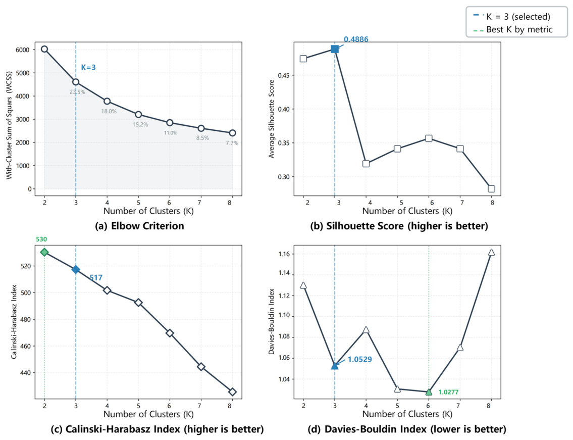
To identify stage-specific differences in the monthly operational states of major airports in Japan, this study implemented the clustering analysis using Python’s scikit-learn library. The raw route-level operational data were first aggregated to the airport-month level, after which the eight state-identification indicators defined in Equations (1)–(8) were calculated. The 2010 observations were retained as the previous-year baseline for calculating the year-on-year indicators for 2011. After excluding observations without a valid previous-year comparison, the final clustering dataset contained 1113 airport-month observations covering January 2011 to March 2024. All indicators were standardized according to Equation (9), and K-means clustering was subsequently applied to the standardized feature set. Candidate solutions from K = 2 to K = 8 were evaluated using four complementary internal validation criteria: the elbow criterion, the average silhouette score, the Calinski–Harabasz index, and the Davies–Bouldin index. Based on the joint consideration of quantitative clustering validity and substantive interpretability, K = 3 was selected as the preferred clustering solution. The cluster distribution, mean feature values, PCA scatter plot, and radar chart were then used to support the substantive interpretation of the identified operational states.

3.2.1. Determination of the Number of Clusters and Clustering Validation

Table 6. Internal clustering validity metrics for candidate solutions (K = 2–8).

K	WCSS/Inertia	WCSS Change (%)	Average Silhouette Score	Calinski–Harabasz Index	Davies–Bouldin Index	Interpretation
2	6027.1	—	0.4744	530.3	1.1302	Under-clustered; substantively distinct states are merged.
3	4608.4	23.5	0.4886	517.3	1.0529	Best balanced solution; selected as the final clustering scheme.
4	3777.3	18.0	0.3193	501.7	1.0875	Over-clustered; cluster separation deteriorates markedly.
5	3204.9	15.2	0.3413	492.6	1.0305	Additional partitions improve compactness slightly, but substantive interpretability weakens.
6	2852.5	11.0	0.3567	469.7	1.0277	Marginal improvement in compactness, but the clustering structure becomes less interpretable.
7	2610.2	8.5	0.3414	444.5	1.0704	Further partitioning yields limited practical benefit and reduced interpretability.
8	2409.0	7.7	0.2821	425.6	1.1617	Excessive partitioning; clustering quality and interpretability both decline.

reports the internal validity metrics for candidate clustering solutions from K = 2 to K = 8. As K increases, WCSS decreases continuously, while the percentage reduction in WCSS becomes progressively smaller, indicating diminishing returns in within-cluster compactness. The average silhouette score reaches its highest value at K = 3 (0.4886), whereas the Calinski–Harabasz index is slightly higher at K = 2 but remains comparably high at K = 3. The Davies–Bouldin index is lower for some higher-K solutions, but these solutions exhibit weaker separation and poorer substantive interpretability. Considering the elbow trend, the silhouette score, the Calinski–Harabasz index, the Davies–Bouldin index, and the interpretability of the resulting states, K = 3 was selected as the final clustering solution.

As shown in Table 6 and Figure 1, K = 3 provides the most balanced solution overall in terms of cluster compactness, separation, and substantive interpretability. Although K = 2 yields a slightly higher Calinski–Harabasz index and K = 6 produces a slightly lower Davies–Bouldin index, K = 3 achieves the highest average silhouette score among all candidate solutions and avoids the marked deterioration in separability observed for K = 4 and higher-K solutions. Therefore, considering both quantitative validity and operational interpretability, K = 3 was selected as the final clustering solution.

Compared with adjacent candidate solutions, the K = 2 solution under-clustered the data by merging substantively distinct airport operational conditions, whereas the K = 4 solution over-clustered the data by splitting the recovery state into highly similar subgroups with limited additional interpretive value. Therefore, the K = 3 solution offers the best compromise between statistical validity and substantive interpretability. A detailed comparison of the clustering structures for K = 2, K = 3, and K = 4 is provided in Appendix A.1.

3.2.2. Clustering Results and State Classification

The monthly state clustering results for all airports are summarized in

Table 7. Distribution of Airport-Month Observations across the Three Operational States.

State	Number of Samples	Proportion (%)
Low-activity state	175	15.72
Recovery state	852	76.55
Rapid-rebound state	86	7.73
Total	1113	100.00

. The results show substantial differences in the number of airport-month observations assigned to each state, indicating that airport operational states are not uniformly distributed over the sample period but exhibit a clear stage-specific structure.

The K = 3 solution classified the 1113 airport-month observations into 175 low-activity-state observations, 852 recovery-state observations, and 86 rapid-rebound-state observations, accounting for 15.72%, 76.55%, and 7.73% of the full clustering sample, respectively. The recovery state therefore represents the predominant operational pattern in the sample, whereas rapid-rebound episodes occur relatively infrequently.

From the perspective of sample distribution, the recovery state is overwhelmingly dominant, suggesting that, for most months during the study period, major Japanese airports remained in a relatively stable operational regime. By contrast, the low-activity and rapid-rebound states account for much smaller proportions, indicating that severe operational contraction and unusually strong rebound were concentrated in specific periods rather than representing normal operating conditions. Overall, the recovery state constitutes the predominant and relatively stable operational condition, the low-activity state primarily corresponds to periods of depressed operations under external shocks, and the rapid-rebound state represents relatively infrequent episodes of exceptionally strong year-on-year growth from a comparatively low operational base.

3.2.3. Differences in State Characteristics and Their Economic Interpretation

To further interpret the substantive meaning of the K-means clustering results, this study compares the mean values of the three identified states across eight indicators, including year-on-year passenger growth, year-on-year flight growth, year-on-year cargo growth, seat utilization rate, weight utilization rate, and the 2019-relative levels of passenger traffic, flights, and cargo. The results are reported in

Table 8. Mean values of the eight indicators across the three identified airport operational states.

State	Year-on-Year Passenger Growth (%)	Year-on-Year Flight Growth (%)	Year-on-Year Cargo Growth (%)	Seat Utilization Rate (%)	Weight Utilization Rate (%)	2019-Relative Passenger Level (%)	2019-Relative Flight Level (%)	2019-Relative Cargo Level (%)
Low-activity state	−29.70	−15.34	−25.72	49.65	35.41	41.59	64.43	63.97
Recovery state	9.51	4.15	2.77	74.40	50.26	93.31	99.42	105.80
Rapid-rebound state	135.61	72.29	87.34	61.54	43.29	64.97	87.71	62.00

.

The cluster-specific mean values reported in Table 8 reveal distinct operational profiles across the three identified states. The low-activity state is characterized by simultaneous contractions in passenger traffic, flight movements, and cargo throughput, with mean year-on-year growth rates of −29.70%, −15.34%, and −25.72%, respectively. Its seat and weight utilization rates are also relatively low, at 49.65% and 35.41%, respectively. In addition, its passenger, flight, and cargo levels correspond to only 41.59%, 64.43%, and 63.97% of their respective 2019 benchmarks, indicating a substantial reduction in overall airport activity.

The recovery state exhibits moderate positive growth in passenger traffic, flight movements, and cargo throughput, with mean year-on-year growth rates of 9.51%, 4.15%, and 2.77%, respectively. It records the highest seat and weight utilization rates among the three states, at 74.40% and 50.26%, respectively. Its passenger and flight levels reach 93.31% and 99.42% of their corresponding 2019 levels, while its cargo level reaches 105.80%. These characteristics indicate relatively stable airport operations that have returned close to the pre-shock benchmark or, in the case of cargo, slightly exceeded it.

The rapid-rebound state is distinguished primarily by exceptionally strong year-on-year growth, with passenger, flight, and cargo growth rates reaching 135.61%, 72.29%, and 87.34%, respectively. However, its seat and weight utilization rates, at 61.54% and 43.29%, remain below those of the recovery state. Its passenger, flight, and cargo levels are equivalent to 64.97%, 87.71%, and 62.00% of their corresponding 2019 levels, respectively. Therefore, the rapid-rebound state reflects a rapid rebound or expansion from a comparatively low operational base, rather than the highest absolute level of airport activity.

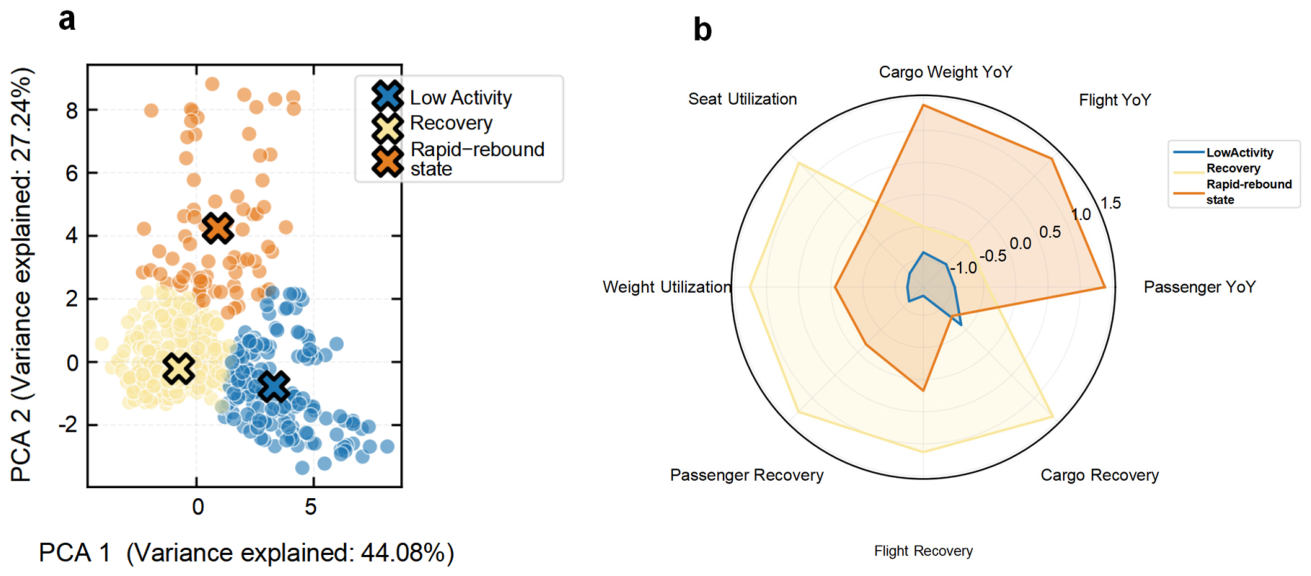
To further examine and validate the plausibility of the clustering results, this study supplements the comparison of mean feature values with a PCA scatter plot and a radar chart of state-specific feature means, thereby providing additional evidence on the separability of the three airport operational states and the structural differences in their indicator profiles. The results are shown in Figure 2.

The PCA scatter plot indicates that the three states exhibit substantial, although not complete, separation in the principal-component space. The low-activity and rapid-rebound states occupy comparatively distinct regions, whereas recovery-state observations are concentrated mainly in the central region and partially overlap with the other two states. This visual pattern is consistent with the internal validation results, including the average silhouette score of 0.4886 for K = 3, which indicates meaningful but not perfect cluster separation. The radar chart further shows that the low-activity state is characterized by negative or weak growth, low utilization rates, and low 2019-relative operational levels; the recovery state records the highest utilization rates and operational levels closest to the 2019 benchmark; and the rapid-rebound state is distinguished primarily by exceptionally strong year-on-year growth from a comparatively depressed operational base. Taken together, the two visualizations support the substantive interpretation of the three clusters, while also indicating that the identified operational states should be understood as empirically distinguishable but not completely discrete operational regimes.

3.2.4. Temporal Evolution Characteristics of Airport Operational States

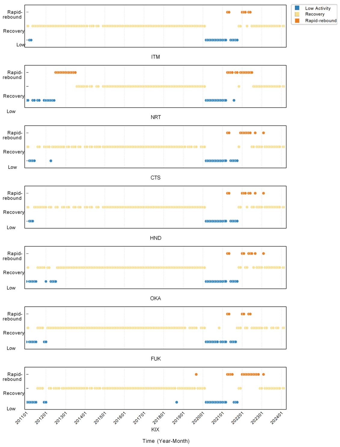
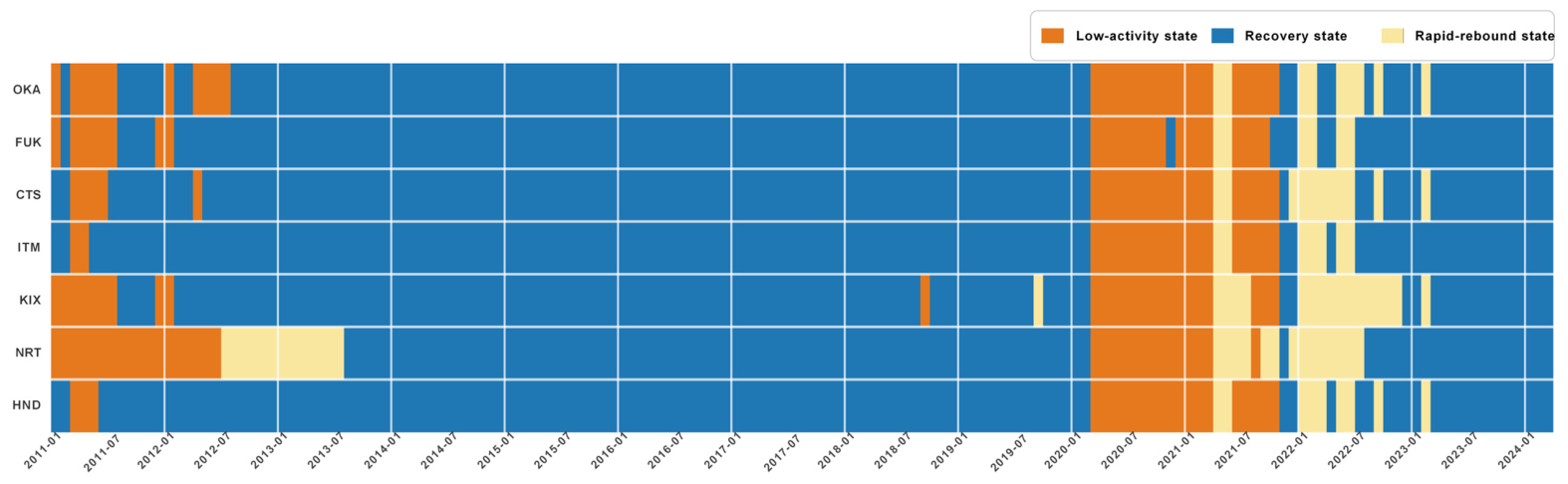
After identifying the three airport operational states, the next step is to examine their evolution over time. To this end, this study analyzes the stage-specific temporal dynamics of major Japanese airports from two complementary perspectives: the state trajectories of individual airports and the overall distribution of states across airports over time. Specifically, the analysis is based on airport-specific state sequence plots and a heatmap of airport states. The corresponding airport-specific state sequences and the overall state heatmap are presented in Figure 3 and Figure 4, respectively.

The airport-specific state sequence plots reveal pronounced stage-specific evolution in the operational states of major Japanese airports. During 2011–2019, most airports remained predominantly in the recovery state for the majority of months, with only occasional fluctuations into the low-activity or rapid-rebound states. This suggests that, prior to the pandemic, airport operations in Japan were generally stable, with the recovery state constituting the dominant long-term operating condition.

From 2020 onward, however, airport operational states changed markedly, as all seven airports shifted into the low-activity state within a relatively similar time frame, indicating that the airport system was substantially affected by external shocks. After the shock, airport operations did not immediately return to a stable condition; instead, most observations gradually shifted from the low-activity state to the recovery state, while some months were classified as belonging to the rapid-rebound state because they exhibited exceptionally strong year-on-year growth and rapid rebound from a lower operational base. The repeated occurrence of the rapid-rebound state around 2021–2022 therefore reflects episodic periods of rapid rebound or expansion rather than the attainment of the highest absolute operational level. By 2023, most airports had returned predominantly to the recovery state, indicating that overall airport operations were gradually regaining stability.

The inclusion of the COVID-19 period is important for identifying the full range of airport operational states, especially the low-activity state and the subsequent recovery process. Nevertheless, the pandemic represents an exceptional and system-wide external shock rather than a routine source of operational fluctuation. Therefore, the state evolution patterns observed during this period should not be interpreted as fully representative of normal operating conditions. In particular, the estimated classification performance may be partly shaped by the sharp contraction and subsequent recovery dynamics associated with the pandemic period. Accordingly, these pandemic-related dynamics are taken into account when interpreting the classification results and are further acknowledged as a limitation of the present study. A sensitivity analysis excluding the pandemic and immediate recovery periods was not conducted because such exclusion would remove most low-activity and rapid-rebound observations, making the resulting state structure and minority-class evaluation statistically unstable.

The results show that, following the external shock, all airports synchronously entered the low-activity state for a prolonged period, exhibiting a high degree of overall consistency. This suggests that the shock had a broad and pervasive impact on the major airport system in Japan. At the same time, airports differed in the timing of their return to the recovery state and in the frequency with which they experienced rapid-rebound episodes, reflecting inter-airport differences in recovery rhythm, fluctuation intensity, and the speed of state transition. Among them, Narita and Kansai airports exhibited the rapid-rebound state relatively more frequently, indicating more pronounced stage-specific rebound characteristics, whereas Haneda, Fukuoka, and Osaka airports returned earlier to an operational pattern dominated by the recovery state, demonstrating relatively stronger stability.

3.2.5. Transition Patterns of Airport Operational States

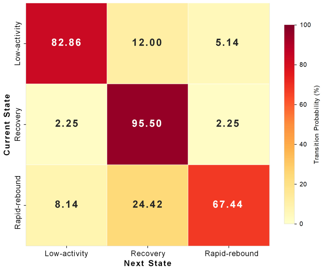
To further reveal the dynamic transition relationships among airport operational states, this study constructs a state transition matrix and visualizes it using a heatmap, as shown in Figure 5, to analyze the transition probabilities among the low-activity, recovery, and rapid-rebound states.

The state transition matrix shows that all three states exhibit some degree of persistence, although their stability differs markedly. The recovery state has the highest self-transition probability, reaching 95.50%, and therefore represents the most persistent operational regime. The self-transition probability of the low-activity state is 82.86%, suggesting that once airports enter a severely depressed operational condition, they tend to remain there for a certain period rather than recover immediately. By contrast, the rapid-rebound state has a substantially lower self-transition probability of 67.44%, confirming that it more often represents a temporary high-growth episode from a comparatively low base than a long-term stable operating condition.

In terms of transition direction, the probability of moving from the low-activity state to the recovery state is 12.00%, which is substantially higher than the probability of moving directly from the low-activity state to the rapid-rebound state (5.14%). This result indicates that observations emerging from severe operational contraction are more likely to enter the relatively stable recovery state than to shift directly into a rapid-rebound episode. The probability of moving from the rapid-rebound state to the recovery state is 24.42%, which is considerably higher than the probability of moving from the rapid-rebound state to the low-activity state (8.14%). Rapid-rebound episodes are therefore more likely to return to the stable recovery regime after a period of unusually strong growth than to deteriorate directly into severe contraction. Overall, the transition structure is centered on a highly persistent recovery state, whereas rapid-rebound episodes are less frequent, less stable, and often followed by a return to recovery. The three states should therefore not be interpreted as a fixed ordinal or linear progression from low activity to recovery and then to a higher operational state.

3.3. Evaluation and Analysis of the Retrospective Airport-State Classification Models

Building on the full-sample state-identification and transition-analysis results, the supervised component evaluates whether retrospectively identified recovery and rapid-rebound labels can be distinguished using lagged operational features. The 60/20/20 chronological partition is applied only to the supervised-classifier stage. Because the target labels were generated through pooled standardization and K-means clustering fitted to the complete sample, and because the 2019-relative variables for pre-2019 observations were constructed using ex post information, the reported metrics assess how well the supervised models reproduce retrospectively identified full-sample labels in chronologically later observations. They do not constitute end-to-end out-of-sample validation or prospective forecasting accuracy.

3.3.1. Comparison of the Overall Classification Performance of Different Models

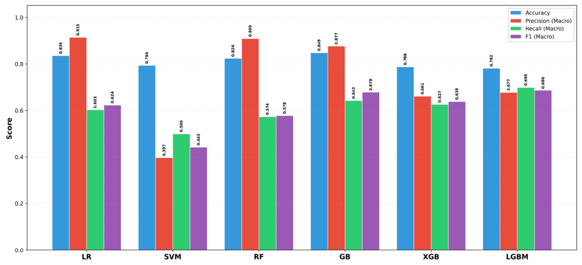
To systematically compare the classification performance of different learning mechanisms, six classification models were evaluated on the same classifier-stage test subset using accuracy, macro-precision, macro-recall, and macro-F1 score. All models were trained and evaluated under the same chronological data partitioning and class-imbalance treatment procedure. The comparative results are presented in Figure 6.

As shown in Figure 6, the six models exhibit considerable differences across the four evaluation metrics. Gradient boosting achieves the highest overall accuracy of 0.8485, followed by logistic regression at 0.8364 and random forest at 0.8242. However, accuracy alone is insufficient for evaluating the present task because the classifier-stage test subset remains imbalanced and the rapid-rebound state represents the minority class.

In terms of balanced classification performance on the current classifier-stage test subset, LightGBM achieves the highest macro-recall of 0.6986 and the highest macro-F1 score of 0.6864 among the six evaluated models. Although its overall accuracy of 0.7818 is lower than that of gradient boosting, logistic regression, and random forest, its higher macro-recall and macro-F1 indicate a more balanced ability to identify both operational states. Gradient boosting ranks second in macro-F1, with a value of 0.6778, whereas XGBoost obtains a macro-F1 score of 0.6387.

Logistic regression and random forest achieve relatively high macro-precision values of 0.9147 and 0.9088, respectively, but their lower macro-recall values indicate that these models produce relatively conservative predictions and fail to identify a substantial proportion of minority-class observations. The RBF-SVM model performs least effectively, particularly in terms of macro-precision and macro-F1. Overall, within the primary SMOTE-based six-model comparison, the evaluated boosting-based models yielded higher point estimates for balanced classification performance than the evaluated linear, kernel-based, and bagging-based models.

To further assess the uncertainty surrounding these point estimates, stratified bootstrap confidence intervals were calculated for the main classification metrics using predictions from the chronologically later test subset. The corresponding results are reported in

Table 9. Bootstrap confidence intervals for the primary SMOTE-based six-model comparison on the classifier-stage test subset.

Model	Accuracy	Macro-Precision	Macro-Recall	Macro-F1	Rapid-Rebound Recall
Logistic Regression	0.8364 [0.8121, 0.8667]	0.9147 [0.9043, 0.9281]	0.6029 [0.5441, 0.6765]	0.6240 [0.5282, 0.7221]	0.2059 [0.0882, 0.3529]
SVM (RBF)	0.7939 [0.7939, 0.7939]	0.3970 [0.3970, 0.3970]	0.5000 [0.5000, 0.5000]	0.4426 [0.4426, 0.4426]	0.0000 [0.0000, 0.0000]
Random Forest	0.8242 [0.8061, 0.8485]	0.9088 [0.9018, 0.9199]	0.5735 [0.5294, 0.6324]	0.5784 [0.5011, 0.6657]	0.1471 [0.0588, 0.2647]
Gradient Boosting	0.8485 [0.8182, 0.8848]	0.8832 [0.7774, 0.9338]	0.6432 [0.5697, 0.7206]	0.6778 [0.5733, 0.7723]	0.2941 [0.1471, 0.4412]
XGBoost	0.7879 [0.7333, 0.8424]	0.6593 [0.5671, 0.7724]	0.6269 [0.5501, 0.7184]	0.6387 [0.5527, 0.7286]	0.3529 [0.2059, 0.5294]
LightGBM	0.7818 [0.7212, 0.8424]	0.6775 [0.6002, 0.7611]	0.6986 [0.6148, 0.7875]	0.6864 [0.6056, 0.7709]	0.5588 [0.4118, 0.7059]

. Compared with point estimates alone, these confidence intervals provide additional evidence regarding the stability and uncertainty of the observed performance differences among the six models.

Values are reported as point estimates [95% bootstrap confidence intervals] for the primary SMOTE-based six-model comparison. The confidence intervals were obtained using 1000 stratified bootstrap resamples of the predictions on the chronologically later test subset. Because individual airport-month observations were resampled within each class, the procedure did not explicitly preserve serial dependence within airports or common month-level dependence across airports. The intervals should therefore be interpreted as conditional empirical uncertainty estimates under the adopted resampling scheme. The degenerate confidence intervals for RBF-SVM arise because the model predicted all test observations as the recovery state, resulting in invariant bootstrap metrics under the stratified resampling procedure.

As shown in Table 9, Gradient boosting obtained the highest point estimate for overall accuracy, whereas LightGBM obtained the highest point estimates for macro-recall, macro-F1, and recall for the rapid-rebound state. However, the confidence intervals indicate that some differences between models, particularly those with similar point estimates, should be interpreted cautiously. The model comparison is therefore reported as evidence of comparative classification performance on the current classifier-stage test subset rather than as definitive proof of statistically universal superiority. The paired bootstrap comparisons between LightGBM and the benchmark models are further reported in Appendix A.3,

Table A3. Paired bootstrap comparisons between LightGBM and benchmark models on the classifier-stage test subset.

Comparison	Δ Macro-F1	95% CI for Δ Macro-F1	Macro-F1 Interpretation	Δ Rapid-Rebound Recall	95% CI for Δ Rapid-Rebound Recall	Rapid-Rebound Recall Interpretation
LightGBM − Logistic Regression	0.0624	[−0.0741, +0.1994]	95% CI includes zero	0.3529	[+0.1176, +0.5882]	95% CI excludes zero
LightGBM − RBF-SVM	0.2438	[+0.1630, +0.3284]	95% CI excludes zero	0.5588	[+0.4118, +0.7059]	95% CI excludes zero
LightGBM − Random Forest	0.1080	[−0.0002, +0.2197]	95% CI includes zero	0.4117	[+0.2647, +0.5882]	95% CI excludes zero
LightGBM − Gradient Boosting	0.0086	[−0.0974, +0.1192]	95% CI includes zero	0.2647	[+0.0882, +0.4412]	95% CI excludes zero
LightGBM − XGBoost	0.0477	[−0.0231, +0.1223]	95% CI includes zero	0.2059	[+0.0882, +0.3529]	95% CI excludes zero

Note: Positive values indicate that LightGBM achieves a higher metric value than the corresponding benchmark model. “95% CI excludes zero” indicates that the confidence interval of the paired difference did not contain zero under the adopted stratified bootstrap procedure, whereas “95% CI includes zero” indicates that the corresponding interval contained zero. Because individual airport-month observations were resampled within each class, the procedure did not explicitly preserve serial dependence within airports or common month-level dependence across airports. These results should therefore be interpreted as conditional empirical comparisons under the adopted resampling scheme rather than as definitive inferential tests.

.

The reported classification performance should be interpreted as classifier-stage performance on chronologically later observations within the present retrospectively constructed dataset. It does not demonstrate that equivalent performance would be achieved in a prospective real-time application using only information available at each historical decision date.

Because the classification objective is not only to maximize overall accuracy but also to identify observations belonging to the less frequent rapid-rebound state, the class-specific recognition performance of the six models is examined further in the following subsection.

3.3.2. Analysis of Model Capability in Identifying the Rapid-Rebound State

Because rapid-rebound states represent relatively infrequent episodes of exceptionally strong year-on-year growth from a comparatively low operational base, identifying them is useful for distinguishing short-term rebound intensity from stable near-normal operation. Accordingly, this subsection focuses on class-specific recognition performance rather than overall accuracy alone. The results show that the six algorithms differ considerably in their ability to identify the minority rapid-rebound state.

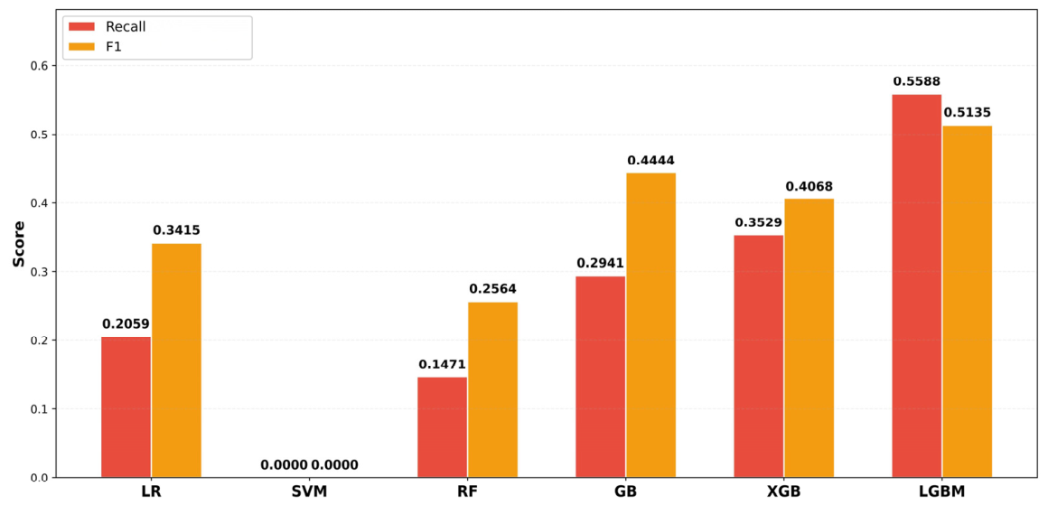
Although several models achieve relatively high recovery-state recognition accuracy because of the larger number of recovery observations, their ability to identify rapid-rebound observations varies substantially, as reflected by the class-specific recall and F1-score comparisons shown in Figure 7.

The zero recall and F1-score values observed for some models indicate that none of the rapid-rebound observations were correctly identified in the classifier-stage test subset. Under the standard definitions of these metrics, recall becomes zero when the number of true positives is zero, and the corresponding F1-score is consequently also zero. These values therefore reflect model classification behavior rather than a metric-calculation failure. Although SMOTE balances the class counts in the training subset through synthetic oversampling, the original training subset contains only seven rapid-rebound observations, which limits the diversity of minority-state patterns available for model learning. Moreover, SMOTE-generated samples cannot provide the same independent information as additional real observations, while the validation and test subsets retain their original imbalanced distributions. Consequently, the zero values reveal the tendency of some classifiers to favor the dominant recovery state and their limited ability to generalize to rare rapid-rebound observations.

The comparatively stronger performance observed for LightGBM in the current experiment may be related to its boosting-based tree structure, which is designed to iteratively focus on difficult-to-classify samples and model nonlinear interactions among lagged growth indicators, operational efficiency variables, and 2019-relative operational-level features. In the present dataset, logistic regression and random forest showed lower minority-class recognition performance than LightGBM. This difference may be associated with the linear specification of logistic regression and the distinct learning mechanism of the bagging-based random forest model.

These results are consistent with the possibility that the retrospective distinction between recovery and rapid-rebound observations involves nonlinear temporal relationships that are not fully captured by the evaluated linear model. Accordingly, models capable of representing nonlinear interactions may assist in the retrospective monitoring of rapid-rebound episodes under data conditions similar to those examined in this study.

3.3.3. Classification Performance and SHAP-Based Interpretation of the LightGBM Model

Based on the primary SMOTE-based six-model reference comparison, LightGBM was selected as the representative model for SHAP-based interpretation because it yielded the highest point estimates for macro-F1 and rapid-rebound-state recall among the six evaluated classifiers. Within this primary SMOTE-based comparison, the paired bootstrap results indicated that the 95% confidence intervals for LightGBM’s differences in rapid-rebound-state recall relative to the benchmark models excluded zero under the adopted stratified resampling scheme, whereas the confidence intervals for its macro-F1 differences relative to several models included zero. These results should be interpreted cautiously because the resampling procedure did not explicitly account for serial dependence within airports or common month-level dependence across airports. Confusion-matrix analysis and SHAP-based feature-attribution analysis were therefore conducted to characterize the classification behavior of the SMOTE-based LightGBM model and to examine how individual features contributed to its fitted distinction between the recovery and rapid-rebound state labels.

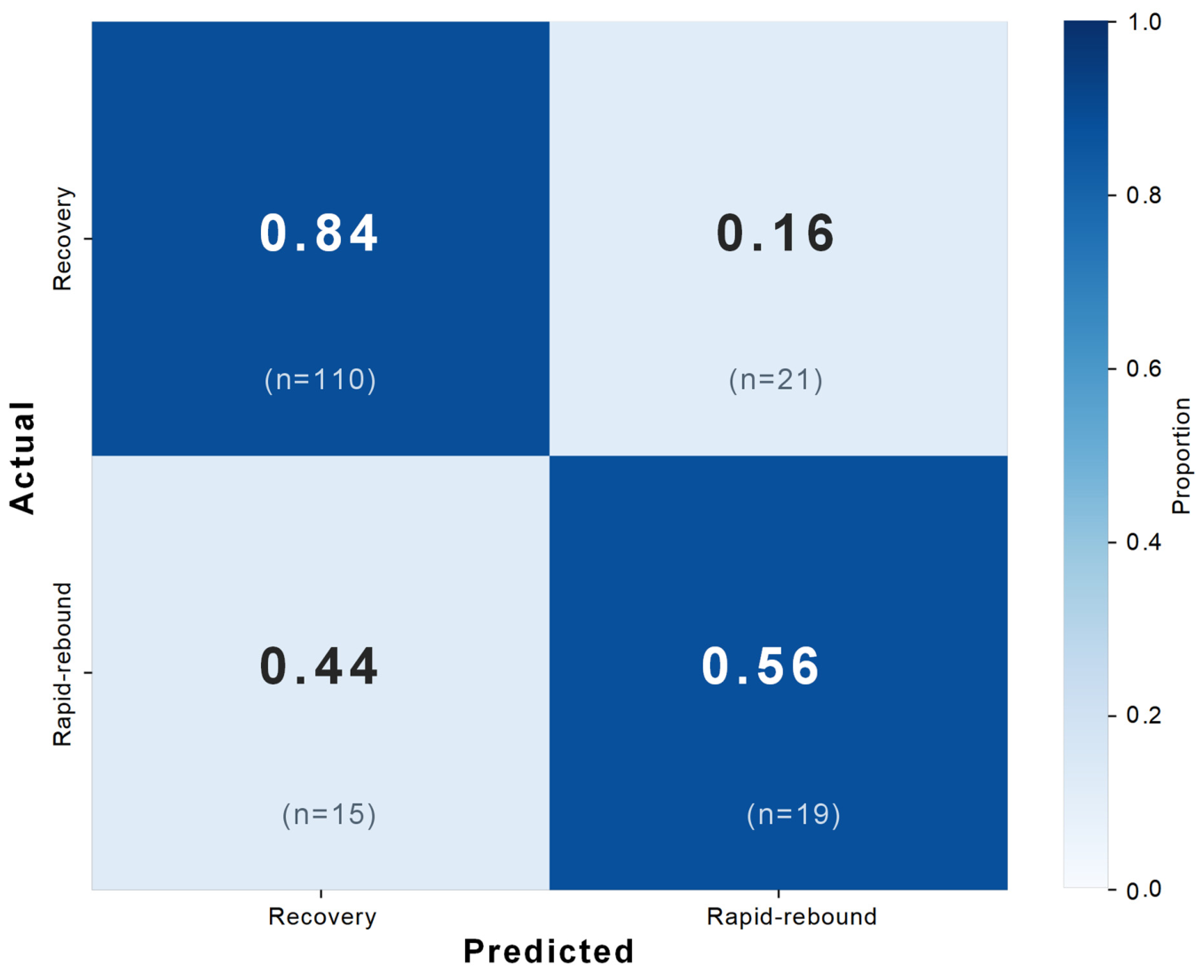
The row-normalized confusion matrix of the LightGBM model is presented in Figure 8. It should be noted that the classifier-stage test subset retained its original class distribution and contained no SMOTE-generated observations. The 34 rapid-rebound observations were original airport-month records, and their relatively large number reflects the temporal concentration of rapid-rebound episodes in the chronologically later post-shock period. On the current classifier-stage test subset, the model correctly classified 110 of the 131 recovery-state observations, corresponding to a recovery-state recall of 0.8397, while 21 recovery-state observations were incorrectly classified as rapid rebound. Among the 34 rapid-rebound-state observations, 19 were correctly identified, corresponding to a rapid-rebound-state recall of 0.5588, whereas 15 were misclassified as recovery. Thus, the four cells in Figure 8 correspond to 0.84 (n = 110), 0.16 (n = 21), 0.44 (n = 15), and 0.56 (n = 19), respectively. Because the classifier-stage test subset contains only 34 rapid-rebound-state observations, the rapid-rebound-state recall should be interpreted together with its 95% bootstrap confidence interval of [0.4118, 0.7059], rather than as an exact estimate of generalizable minority-state recognition performance.

The asymmetric classification pattern suggests that identifying rapid-rebound observations remains more challenging than identifying recovery observations. This result is plausible because the rapid-rebound state is defined primarily by unusually strong year-on-year growth from a comparatively low base, while some of its utilization rates and benchmark-relative operational levels may overlap with those observed during recovery. The partially shared feature distributions between the two states therefore make rapid-rebound observations more difficult to distinguish consistently.

Compared with the benchmark models that predominantly classified observations into the majority recovery state, LightGBM correctly identified a larger number of rapid-rebound observations in the current classifier-stage test subset. Within the present comparison, this result suggests that the fitted boosting-based model may represent interactions among lagged growth indicators, operational-efficiency variables, and 2019-relative operational-level features more effectively than the specific benchmark models evaluated in this study.

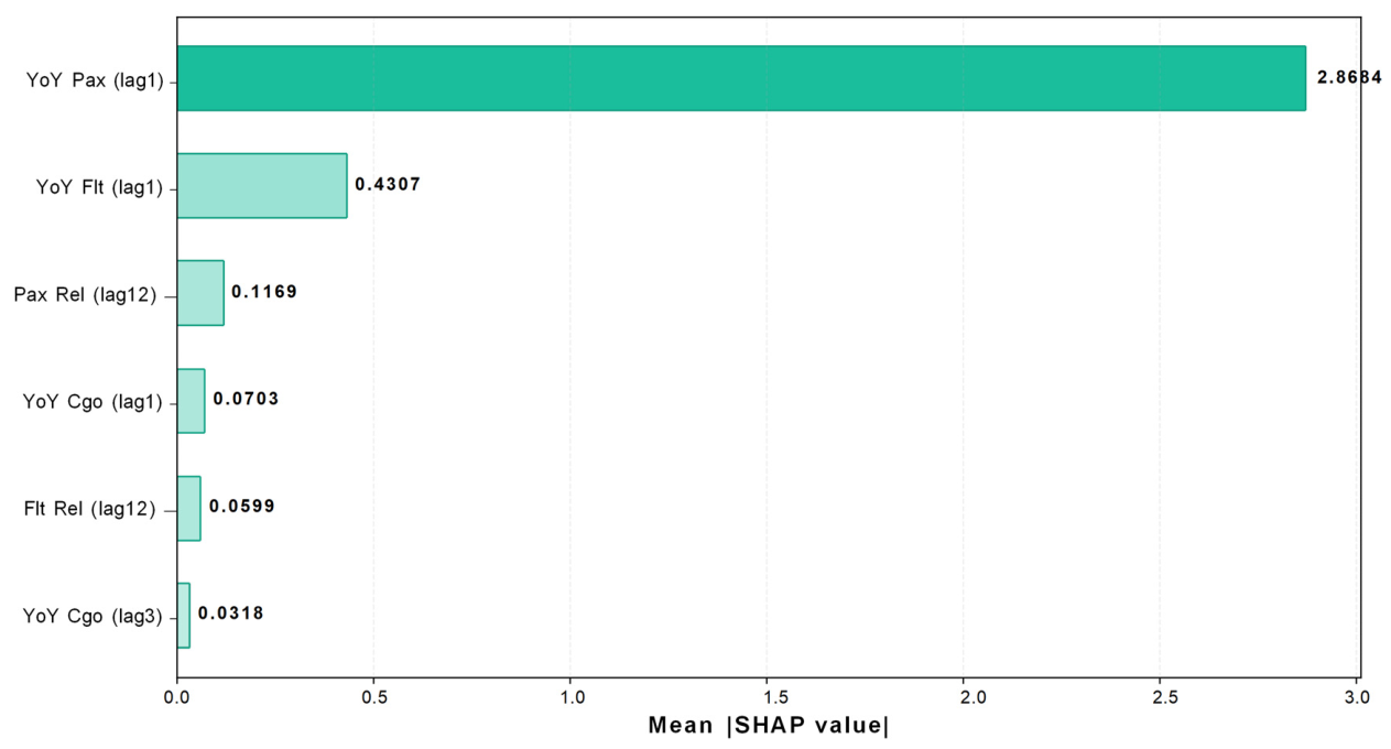
To further characterize how the fitted LightGBM model uses the input variables, SHAP analysis is employed to quantify the contribution of individual features to the fitted distinction between the recovery and rapid-rebound state labels. SHAP values reflect model-specific feature contributions and associations rather than causal effects. Accordingly, features with larger absolute SHAP values are interpreted as contributing more strongly to the fitted classification output, rather than as causally driving changes in airport operational states. The SHAP-based ranking of feature contributions is presented in Figure 9.

The SHAP ranking indicates that short-term lagged growth indicators and twelve-month 2019-relative operational-level variables make relatively large contributions to the LightGBM classification results. In particular, the dominant contribution of the one-month lag of passenger growth is consistent with the defining characteristic of the rapid-rebound state: exceptionally strong year-on-year growth from a comparatively low operational base. The contributions of the twelve-month 2019-relative variables further indicate that the fitted model distinguishes rebound intensity jointly with the airport’s longer-term operational position relative to the 2019 benchmark. These SHAP results should therefore be interpreted as explaining the fitted distinction between recovery and rapid-rebound observations, rather than as indicating movement toward a higher absolute operational level.

3.3.4. Exploratory Sensitivity Analysis Under Alternative Class-Imbalance Handling Strategies

To examine the sensitivity of the classification point estimates to the selected class-imbalance treatment, an exploratory analysis was conducted using SMOTE, random oversampling, and class-weighted learning. Rather than repeating the complete six-model comparison, three representative classifiers were included to cover distinct learning mechanisms: logistic regression as a linear classifier, random forest as a bagging-based ensemble classifier, and LightGBM as a boosting-based classifier. For the random-oversampling and class-weighted variants, the hyperparameter configurations selected under the primary SMOTE-based validation procedure were retained, and no strategy-specific hyperparameter retuning was performed. All variants were evaluated on the same chronologically later test subset. Therefore, this analysis examines changes in point estimates under alternative imbalance treatments and should not be interpreted as a fully optimized comparison of imbalance-handling strategies or as a second model-selection procedure.

This exploratory sensitivity analysis was conducted after the primary SMOTE-based procedure had been fixed and was not used to redefine the primary model-selection process. Promoting the class-weighted specification to the primary analysis solely on the basis of its higher point estimates on the test subset would constitute post hoc outcome-driven model selection.

The exploratory sensitivity results are reported in

Table 10. Exploratory Sensitivity Comparison of Alternative Class-Imbalance Handling Strategies for Retrospective Airport-State Classification.

Model	Strategy	Accuracy	Macro-F1	Rapid-Rebound F1	Rapid-Rebound Recall
Logistic Regression	SMOTE	0.8364	0.6240	0.3415	0.2059
Logistic Regression	ROS	0.8364	0.6240	0.3415	0.2059
Logistic Regression	Class-Weighted	0.8182	0.5539	0.2105	0.1176
Random Forest	SMOTE	0.8242	0.5784	0.2564	0.1471
Random Forest	ROS	0.8242	0.5784	0.2564	0.1471
Random Forest	Class-Weighted	0.8242	0.5784	0.2564	0.1471
LightGBM	SMOTE	0.7818	0.6864	0.5135	0.5588
LightGBM	ROS	0.7818	0.6864	0.5135	0.5588
LightGBM	Class-Weighted	0.8970	0.8609	0.7901	0.9412

Notes: ROS denotes random oversampling. The class-weighted variants used inverse-frequency balanced weights calculated from the original training-set class distribution. The ROS and class-weighted variants retained the hyperparameter configurations selected under the primary SMOTE-based validation procedure, and no strategy-specific hyperparameter retuning was performed. All reported values are point estimates on the chronologically later test subset. Strategy-specific bootstrap confidence intervals and paired statistical comparisons were not conducted for this exploratory analysis.

. For logistic regression, SMOTE and random oversampling produced identical point estimates, with an accuracy of 0.8364, a macro-F1 score of 0.6240, and rapid-rebound-state recall of 0.2059. Under class-weighted learning, macro-F1 decreased to 0.5539 and rapid-rebound-state recall decreased to 0.1176. Thus, within the fixed hyperparameter configuration used in this exploratory analysis, changing from resampling to inverse-frequency class weighting did not improve minority-state recognition for logistic regression. This result applies to the present implementation and should not be interpreted as general evidence against class weighting or as proof that the underlying airport-state distinction is inherently nonlinear.

Random forest produced identical point estimates under the three evaluated imbalance-handling strategies, with an accuracy of 0.8242, a macro-F1 score of 0.5784, and rapid-rebound-state recall of 0.1471. The model maintained relatively strong recognition of the recovery state but identified only a small proportion of rapid-rebound observations. Under the fixed hyperparameter configuration retained from the primary SMOTE-based procedure, the random forest results were therefore relatively insensitive to the three evaluated imbalance treatments, although minority-state recognition remained limited.

For LightGBM, SMOTE and random oversampling produced the same point estimates, including a macro-F1 score of 0.6864 and rapid-rebound-state recall of 0.5588. The class-weighted LightGBM specification yielded point estimates of 0.8970 for accuracy, 0.8609 for macro-F1, and 0.9412 for rapid-rebound-state recall. Its confusion matrix indicated that 32 of the 34 rapid-rebound observations were correctly classified, while recovery-state recall remained 0.8855. These point estimates were materially higher than those obtained under SMOTE and random oversampling. However, because the class-weighted specification retained hyperparameters selected under the primary SMOTE-based procedure and was not accompanied by strategy-specific retuning or equivalent bootstrap uncertainty assessment, the observed differences should not be interpreted as statistically established superiority of class-weighted LightGBM.

Overall, the exploratory analysis indicates that estimated classification performance, particularly rapid-rebound-state recall, is materially sensitive to the selected imbalance-handling strategy. The results do not confirm the robustness of the primary SMOTE-based estimates, nor do they establish class-weighted learning as the optimal strategy. Instead, they identify imbalance treatment as an important source of methodological uncertainty in the present setting, where only seven rapid-rebound observations were available in the original training subset. The higher point estimates obtained by class-weighted LightGBM suggest that direct loss weighting may warrant further investigation, but a definitive comparison would require strategy-specific hyperparameter tuning, application to the complete set of candidate classifiers, and equivalent confidence-interval or paired-bootstrap assessment.

From a managerial perspective, the rapid-rebound state should not be interpreted automatically as a superior operational condition or as evidence of complete recovery. Its exceptionally high year-on-year growth occurs alongside utilization rates and 2019-relative operational levels that remain below those of the recovery state. Airport managers should therefore distinguish rebound speed from recovery level and should jointly consider growth momentum, resource utilization, and benchmark-relative operational position when assessing recovery progress. A rapid-rebound classification may indicate a need to monitor whether short-term demand growth can be converted into a stable recovery regime; by itself, however, it does not justify permanent capacity expansion or long-term resource commitments.

4. Conclusions

Using seven major Japanese airports as empirical cases, this study developed a two-stage analytical framework for airport operational-state identification, temporal evolution analysis, and retrospective classification. The framework combines unsupervised learning for latent-state discovery with supervised learning for distinguishing ex post-defined operational-state labels in chronologically later observations. Three operational states—the low-activity state, recovery state, and rapid-rebound state—were identified from multidimensional indicators reflecting growth dynamics, operational efficiency, and 2019-relative operational level. The recovery state exhibits the highest utilization rates and operational levels closest to the 2019 benchmark, whereas the rapid-rebound state is characterized by exceptionally strong year-on-year growth from a comparatively low operational base. The rapid-rebound state therefore does not represent the highest absolute operational level or a superior stage beyond recovery.

The transition analysis shows that the recovery state is the most persistent operational regime, with a self-transition probability of 95.50%, whereas the rapid-rebound state is less stable, with a self-transition probability of 67.44%. Transitions from low activity are more likely to enter the recovery state than to move directly into rapid rebound, and rapid-rebound episodes frequently return to recovery. The observed state structure therefore does not support a simple linear progression from low activity through recovery to a higher final state. Instead, it is centered on a highly persistent recovery regime, with intermittent rapid-rebound episodes reflecting unusually strong growth from a depressed base.

The supervised analysis was restricted to distinguishing recovery and rapid-rebound observations because low-activity observations were temporally concentrated around the external-shock period and provided insufficient repeated patterns for stable supervised learning. Under the prespecified common SMOTE-based six-model comparison, Gradient Boosting yielded the highest point estimate for accuracy, reaching 0.8485, whereas LightGBM yielded the highest point estimates for macro-F1 and rapid-rebound-state recall, reaching 0.6864 and 0.5588, respectively. Because the original training subset contained only seven rapid-rebound observations, the SMOTE-generated samples were necessarily derived from a very limited set of observed minority-class cases, and the corresponding results should therefore be interpreted cautiously. The exploratory sensitivity analysis produced materially different point estimates across imbalance-handling strategies, indicating that minority-state classification performance is sensitive to the selected treatment. Accordingly, the supervised results should be regarded as preliminary evidence of temporal separability rather than as a definitive selection of an optimal classifier or imbalance-handling method.

From a methodological perspective, this study integrates latent-state identification, state-transition analysis, class-imbalance treatment, classifier-stage evaluation on chronologically later observations, and feature-attribution analysis within a unified framework. From an applied perspective, the distinction between recovery and rapid rebound demonstrates that exceptionally high growth does not necessarily indicate the highest operational level or complete recovery. The framework can support retrospective comparison of recovery trajectories and help distinguish short-term rebound intensity from stable near-normal operation. Although the framework was developed using major Japanese airports, its general analytical structure may be transferable to airport systems in other countries where consistent monthly data on passenger traffic, flight activity, cargo throughput, capacity, and resource utilization are available. However, the operational-state definitions, reference benchmarks, standardization parameters, and cluster centroids would need to be re-estimated and externally validated for each regional airport system rather than being directly transferred from the Japanese sample. Importantly, the proposed framework is intended as a retrospective analytical framework for airport operational-state identification and assessment, rather than as a fully prospective, deployable real-time prediction or early-warning system. Upstream pooled standardization, selection of K, and estimation of the K-means cluster centroids were conducted using the complete 2010–2024 sample, while the 2019-relative variables for pre-2019 observations also relied on an ex post benchmark. Consequently, observations in the chronologically later validation and test periods contributed to the retrospective construction of the target state labels, although they were not used for supervised-model fitting, SMOTE processing, or hyperparameter selection. The reported classification results therefore represent classifier-stage temporal evaluation of retrospectively identified full-sample labels rather than end-to-end out-of-sample validation. Future research should estimate the standardization parameters, select K, and determine the cluster centroids using training-period data only, assign later observations to the fixed training-derived centroids, reconstruct all input variables using information available at each forecast origin, and evaluate the complete pipeline using rolling-origin or time-series cross-validation. Beyond such end-to-end prospective validation, future studies may also examine anomaly-detection approaches for airport operational monitoring by defining a normal reference regime, establishing appropriate anomaly-score thresholds, and evaluating deviations under a rolling-origin validation framework.

References

1. Yu, C. Airport performance—A multifarious review of literature. J. Air Transp. Res. Soc. 2023, 1, 22–39. [Google Scholar] [CrossRef]
2. Sarkis, J. An analysis of the operational efficiency of major airports in the United States. J. Oper. Manag. 2000, 18, 335–351. [Google Scholar] [CrossRef]
3. Choi, J.H. Changes in airport operating procedures and implications for airport strategies post-COVID-19. J. Air Transp. Manag. 2021, 94, 102065. [Google Scholar] [CrossRef] [PubMed]
4. Janic, M. Modeling airport operations affected by a large-scale disruption. J. Transp. Eng. 2009, 135, 206–216. [Google Scholar] [CrossRef]
5. Yang, L.; Wang, Y.; Liu, S.; Wang, M.; Wang, S.; Ren, Y. Multi-airport capacity decoupling analysis using hybrid and integrated surface–airspace traffic modeling. Aerospace 2025, 12, 237. [Google Scholar] [CrossRef]
6. Zhu, Z.; Okuniek, N.; Gerdes, I.; Schier, S.; Lee, H.; Jung, Y. Performance evaluation of the approaches and algorithms for Hamburg Airport operations. In Proceedings of the 2016 IEEE/AIAA 35th Digital Avionics Systems Conference (DASC); IEEE: New York, NY, USA, 2016; pp. 1–10. [Google Scholar] [CrossRef]
7. Li, W.K.; Miyoshi, C.; Pagliari, R. Dual-hub network connectivity: An analysis of All Nippon Airways’ use of Tokyo’s Haneda and Narita airports. J. Air Transp. Manag. 2012, 23, 12–16. [Google Scholar] [CrossRef]
8. Hanaoka, S. Air transport in Japan: Demand, policy making, and slot allocation at Haneda airport. In Research Handbook on Air Transport Leadership and Governance; Edward Elgar Publishing: Cheltenham, UK, 2025; pp. 60–70. [Google Scholar] [CrossRef]
9. Ha, H.K.; Yoshida, Y.; Zhang, A. Comparative analysis of efficiency for major Northeast Asia airports. Transp. J. 2010, 49, 9–23. [Google Scholar] [CrossRef]
10. Oktal, H.; Özger, A. Hub location in air cargo transportation: A case study. J. Air Transp. Manag. 2013, 27, 1–4. [Google Scholar] [CrossRef]
11. Tsuzaki, T. Air transport in Hokkaido region. Stud. Reg. Sci. 1975, 6, 151–160. [Google Scholar] [CrossRef]
12. Wiredja, D.; Popovic, V.; Blackler, A. A passenger-centred model in assessing airport service performance. J. Model. Manag. 2019, 14, 492–520. [Google Scholar] [CrossRef]
13. Wen, J.; Xiao, Y.C.; Feng, Q. Research on airport passenger throughput prediction based on Euclidean distance. In Proceedings of the Sixth International Conference on Traffic Engineering and Transportation System (ICTETS 2022), Guangzhou, China, 23–25 September 2022; Zhou, J., Sheng, J., Eds.; SPIE: Bellingham, WA, USA, 2023; Volume 12591, Article No. 125912I. [Google Scholar] [CrossRef]
14. Zhang, Z.N.; Meng, F.S. Multi-airport flight delay propagation analysis based on complex networks. Sci. Technol. Eng. 2024, 24, 7913. (In Chinese) [Google Scholar] [CrossRef]
15. Hu, M.H.; Yi, T.Y.; Ren, Y.M. Research on airport flight slot optimization based on improved Hungarian algorithm. Appl. Res. Comput. 2019, 36, 2039. (In Chinese) [Google Scholar] [CrossRef]
16. Yang, C.H.; Shao, J.C.; Liu, Y.H.; Hsueh, Y.H.; Chou, C.C. Application of fuzzy-based support vector regression to forecast of international airport freight volumes. Mathematics 2022, 10, 2399. [Google Scholar] [CrossRef]
17. Chen, B.; Wu, J. Airport traffic demand prediction method based on large sample data. Syst. Eng. Electron. 2023, 45, 3887. (In Chinese) [Google Scholar] [CrossRef]
18. Nikolaou, P.; Dimitriou, L. Investigating and identifying critical airports for controlling infectious diseases outbreaks. Transp. Res. Procedia 2021, 52, 437–444. [Google Scholar] [CrossRef]
19. Nikolaou, P.; Dimitriou, L. Identification of critical airports for controlling global infectious disease outbreaks: Stress-tests focusing in Europe. J. Air Transp. Manag. 2020, 85, 101819. [Google Scholar] [CrossRef] [PubMed]
20. He, J.; Guo, H.Y.; Yao, Y.; Bian, L.; Tang, H.W.; Wang, D.S. Irregular flight recovery technology based on effective transfer time prediction. J. Beijing Univ. Aeronaut. Astronaut. 2022, 48, 384–393. (In Chinese) [Google Scholar] [CrossRef]
21. Zhang, H.Y.; Wu, W.W.; Hua, H.; Guo, Y.M. Evolutionary characteristics of China’s international air route network under COVID-19. J. Beijing Univ. Aeronaut. Astronaut. 2023, 49, 2699–2710. (In Chinese) [Google Scholar] [CrossRef]
22. Wu, W.; Lin, Z.Y.; Wang, X.L. Evolutionary game of multi-airport route network under subsidy strategy in homogeneous competition. J. Beijing Univ. Aeronaut. Astronaut. 2025, 51, 3392–3404. (In Chinese) [Google Scholar] [CrossRef]
23. Esmaeilzadeh, E.; Mokhtarimousavi, S. Machine learning approach for flight departure delay prediction and analysis. Transp. Res. Rec. J. Transp. Res. Board 2020, 2674, 145–159. [Google Scholar] [CrossRef]
24. Kim, S.; Shin, D.H. Forecasting short-term air passenger demand using big data from search engine queries. Autom. Constr. 2016, 70, 98–108. [Google Scholar] [CrossRef]
25. Abdelghany, A.; Guzhva, V. A time-series modelling approach for airport short-term demand forecasting. J. Airpt. Manag. 2010, 5, 72–87. [Google Scholar] [CrossRef]
26. He, X.N.; Li, Y.H.; Yang, J. Optimization model of dual-hub route network based on competitive scenarios. J. Beijing Univ. Aeronaut. Astronaut. 2024, 50, 2902–2911. (In Chinese) [Google Scholar] [CrossRef]
27. Fu, C.Q.; Wang, Y.; Li, C.; Sun, Y. Self-healing characteristics of aviation network under different growth mechanisms. J. Beijing Univ. Aeronaut. Astronaut. 2018, 44, 1221–1229. (In Chinese) [Google Scholar] [CrossRef]
28. Azzam, M. Evolution of airports from a network perspective—An analytical concept. Chin. J. Aeronaut. 2017, 30, 513–522. [Google Scholar] [CrossRef]
29. Maertens, S.; Grimme, W.; Bingemer, S. The development of transfer passenger volumes and shares at airport and world region levels. Transp. Res. Procedia 2020, 51, 171–178. [Google Scholar] [CrossRef]
30. Yang, C.H.; Lee, B.; Jou, P.H.; Chung, Y.F.; Lin, Y.D. Analysis and forecasting of international airport traffic volume. Mathematics 2023, 11, 1483. [Google Scholar] [CrossRef]
31. Likas, A.; Vlassis, N.; Verbeek, J.J. The global k-means clustering algorithm. Pattern Recognit. 2003, 36, 451–461. [Google Scholar] [CrossRef]
32. Rao, A.R.; Wang, H.; Gupta, C. Predictive Analysis for Optimizing Port Operations. Appl. Sci. 2025, 15, 2877. [Google Scholar] [CrossRef]
Figure 1. Determination of the optimal number of clusters for K-means clustering: (a) elbow criterion; (b) silhouette score; (c) Calinski–Harabasz index; and (d) Davies–Bouldin index.
Mathematics 14 02732 g001
Figure 2. Visual interpretation of the clustering results: (a) PCA scatter plot of airport-month samples; (b) radar chart of mean feature values across states.
Mathematics 14 02732 g002
Figure 3. Temporal sequence of airport operational states.
Mathematics 14 02732 g003
Figure 4. Heatmap of airport operational states.
Mathematics 14 02732 g004
Figure 5. Heatmap of the airport operational state transition matrix.
Mathematics 14 02732 g005
Figure 6. Performance comparison of the six classification models on the classifier-stage test subset under the chronological 60/20/20 data split.
Mathematics 14 02732 g006
Figure 7. Recall and F1-score comparison for rapid-rebound state recognition across six classification models.
Mathematics 14 02732 g007
Figure 8. Row-normalized confusion matrix for the LightGBM model on the original, unresampled classifier-stage test subset.
Mathematics 14 02732 g008
Figure 9. SHAP-based ranking of feature contributions in the fitted LightGBM model.
Mathematics 14 02732 g009