A Projection-Free Sparse Model Order Reduction Method for Thermomechanical Multibody Dynamics

Abstract

Thermomechanical coupling effects significantly influence the dynamic response of flexible multibody systems operating in thermal environments. Accurate simulation using conventional projection-based reduced-order models remains challenging due to strong nonlinearity and the time-varying nature of thermal fields. This work proposes a projection-free sparse-solving framework for thermomechanical coupling dynamics. The elastic and thermal fields are represented using sparse POD coefficients, and the governing equations are directly sampled online without Galerkin projection. The sparse coefficients are recovered via l₁ norm optimization at each time step. To ensure stable recovery under thermal-mechanical coupling, a unit-norm tight frame-based preconditioner is introduced to reduce the coherence of the underdetermined system matrix. The proposed method is validated through three numerical examples. Results show that the method maintains stable accuracy over long-time simulations, reduces computational time by over 40%, and exhibits improved robustness compared with the discrete empirical interpolation method in thermomechanical coupling problems. The adaptive basis selection capability and the necessity of unit norm tight frame preconditioning are confirmed. The method offers an efficient and reliable alternative for thermomechanical multibody dynamics simulation.

1. Introduction

Flexible multibody systems are widely used across various engineering fields to model mechanical systems, including aerospace, robotics, and automotive applications. As these systems become increasingly sophisticated and operate in diverse environments, it is essential to consider multiple factors to ensure accurate analysis and design. Among these factors, thermal expansion alters material stiffness and induces stress gradients, thereby modifying the dynamic response of flexible bodies. Thermal phenomena are common in many engineering applications, including brake disk systems [1,2], machine tool systems [3,4], and aircraft systems [5,6]. Consequently, thermomechanical coupling has become a growing area of research interest in recent years [7,8,9,10,11].

For analyzing thermomechanical coupling systems, the finite element method (FEM) has long been the standard tool for modeling and predicting dynamic responses [12,13,14,15]. However, when the system involves significant rotational motion or kinematic joint constraints, the nonlinear inertial effects dramatically increase the computational cost. Furthermore, reducing element size to improve numerical accuracy increases the degrees of freedom (DOF), thereby exacerbating the computational burden.

To address these challenges, model order reduction (MOR) techniques have been developed as computational strategies to reduce system dimensionality while preserving essential dynamic characteristics [16,17]. The fundamental principle of MOR is to select optimal basis functions that span the solution spaces of deformation and temperature fields in thermomechanical systems. Through mathematical projection techniques such as the Galerkin method, these basis functions enable the construction of reduced-order dynamic models [18,19,20]. Prominent MOR approaches include modal truncation [21,22], moment matching [23,24], and proper orthogonal decomposition (POD) [25,26,27,28]. In modal truncation, structural mode shapes obtained from eigenvalue analysis are employed to approximate the coupled deformation-temperature fields. Nevertheless, the inherent thermal coupling introduces nonsymmetric stiffness matrix components that violate the orthogonality condition required for conventional modal superposition [29]. This limitation necessitates the inclusion of additional mode shapes to satisfy multiphysics boundary conditions, including mechanical constraints (joint forces or external loads) and thermal excitation conditions (heat sources). This inherent limitation of mode superposition methods motivates the use of data-driven alternatives. The POD-based approach constructs empirical basis functions by performing a singular value decomposition (SVD) of snapshot matrices obtained from numerical simulations or experimental measurements [18,30]. However, the Galerkin projection step that follows POD still requires operations on the full-order system matrices, which become computationally expensive for nonlinear problems, thereby diminishing the overall efficiency gains expected from model reduction. To address this issue, hyper-reduction techniques have been developed. Hyper-reduction methods can be broadly classified into two categories [31]. Approximate-then-project methods (AP), such as the discrete empirical interpolation method (DEIM) and Gauss-Newton with approximate tensors (GNAT)—first approximate the nonlinear terms in the full order space using interpolation at strategically selected sampling points, and then project these approximations onto the reduced subspace [32]. Project-then-approximate (PA) methods, such as the energy-conserving sampling and weighting (ECSW) and the empirical cubature method (ECM)—first project the governing equations onto the reduced subspace and then approximate the resulting projected integrals using reduced quadrature rules on a sample mesh [33].

Despite their effectiveness, hyper-reduction methods face three fundamental limitations common to both categories [31]. First, they impose high offline data requirements: beyond the state-variable snapshots needed for standard POD methods, AP methods require nonlinear force snapshots, while PA methods require element-level nonlinear forces, doubling the computational cost and storage requirements. Second, the singular values of the data used to construct the approximation bases often decay slowly for strongly nonlinear or multiphysics problems, necessitating a large number of sampling points to achieve acceptable accuracy. When the number of sampling points approaches the full-order model size, the efficiency gain vanishes, and AP methods such as DEIM can also suffer from numerical instability when the selected points yield an ill-conditioned interpolation matrix. Third, in both AP and PA methods, the sampling points are selected offline via deterministic algorithms and remain fixed throughout the online phase, offering no adaptability to evolving system dynamics—a critical shortcoming for thermomechanical coupling problems where the active regions of thermal and mechanical fields shift over time. These limitations motivate the development of alternative paradigms that circumvent the Galerkin projection framework, eliminate the need for nonlinear force snapshots, and offer greater flexibility in sampling.

To overcome these limitations, compressive sensing (CS) has emerged as a promising alternative for model reduction [34,35], enabling the recovery of sparse solutions from underdetermined systems without relying on offline-fixed subspaces [36]. A preliminary version of this CS-based framework was developed in our previous work for purely flexible multibody systems using modal bases [37]. However, the direct extension to thermomechanical coupling is nontrivial for two reasons. First, modal bases are derived from linearized eigenvalue analysis and lack the capacity to capture the evolving thermal subspace, making them unsuitable for problems with thermal effects. Second, the coupling between the thermal and mechanical fields introduces high coherence in the system matrix, undermining the stability of l₁ recovery.

In this article, we propose a fundamentally different paradigm for nonlinear model reduction. In contrast to both AP and PA hyper-reduction methods, which either approximate-then-project or project-then-approximate, the proposed framework completely bypasses Galerkin projection. Instead of approximating nonlinear terms at any stage, it directly samples the full-order governing equations online, including their nonlinear terms, and recovers the coefficients via compressed sensing, thereby avoiding explicit approximation of the nonlinearities. The key idea is to represent the solution using POD basis vectors, assuming the corresponding coefficients are sparse. It is worth noting that the framework itself is not restricted to POD and supports any basis that provides a sparse representation of the state variables, including overcomplete and traditional bases. This sparsity assumption enables the use of l₁ norm optimization to reconstruct the entire dynamic response from a small number of sampled equations.

A key challenge in compressed sensing is the high coherence of the measurement matrix, which can significantly degrade the performance of the sparse recovery algorithm [35,36]. The underdetermined system of equations arising from the online sampling strategy is analogous to a compressed sensing measurement system, where the coefficient matrix also exhibits high coherence. This coherence is further exacerbated by the coupling between thermal and mechanical fields in thermomechanical systems, leading to an ill-conditioned recovery problem. To address this coherence issue, preconditioning is an effective strategy for reducing the coherence of underdetermined linear systems in sparse recovery [38,39,40]. Recent advances have extended this idea by transforming the system matrix into an incoherent unit-norm tight frame (UNTF), a structure known to facilitate stable sparse recovery [38,39]. Inspired by these developments, we construct a UNTF-based preconditioner that reduces the coherence of the sampled thermomechanical system matrix without increasing its dimension. This preconditioning strategy stabilizes the l₁ solver, ensuring robust and accurate recovery for thermomechanical coupling problems.

The main contributions of this article are summarized as follows.

(1)

A projection-free sparse-solving paradigm is proposed for nonlinear model reduction, where the full-order discretized equations are directly sampled online and the reduced coefficients are recovered via compressed sensing. The paradigm eliminates the need for Galerkin projection and nonlinear force snapshots, and is extended to thermomechanical coupling by adopting data-driven bases for sparse representation of both elastic and thermal fields.

(2)

A UNTF-based preconditioning strategy is developed to address the high coherence of the underdetermined system matrix arising from the sampled thermomechanical equations, ensuring stable and accurate l₁ solver convergence.

The remainder of this paper is organized as follows. Section 2 introduces the background on thermomechanical dynamics, the POD method, and the l₁ norm optimization. Section 3 derives the sparse POD coefficients l₁ norm problem constrained by a few thermomechanical coupling dynamic equations and presents the UNTF-based preconditioning procedure. Section 4 validates the proposed method with numerical examples. Finally, Section 5 concludes the paper with a summary of the key findings.

2. Background

This section reviews the background of thermomechanical coupling dynamic systems. Then, the background of proper orthogonal decomposition (POD), the l₁ norm optimization, and the discrete empirical interpolation method (DEIM) are presented.

2.1. Thermomechanical Dynamic Equations

2.1.1. Flexible Body Motion Equations

Considering a multibody system consisting of N_b flexible bodies, the motion equations of the ith flexible body, where i = 1, 2, …, N_b, can be written as [41]:

$${\mathit{M}}^i({\mathit{q}}^i){\ddot{\mathit{q}}}^i+{\mathit{K}}^i{\mathit{q}}^i+{\mathit{G}}^T({\mathit{q}}^i)\mathit{\lambda }-{\mathit{Q}}_e^i({\mathit{q}}^i,{\dot{\mathit{q}}}^i,t)-{\mathit{Q}}_v^i({\mathit{q}}^i,{\dot{\mathit{q}}}^i)=\mathbf{0}$$

(1)

where ${\mathit{q}}^i$ represents the generalized coordinates, which consist of the rigid coordinates ${\mathit{q}}_r^i$ and elastic coordinates ${\mathit{q}}_f^i$. These components describe the rigid-body motion and the elastic deformation, respectively. The velocity and acceleration of the generalized coordinates are denoted as ${\dot{\mathit{q}}}^i$ and ${\ddot{\mathit{q}}}^i$, respectively. The mass matrix ${\mathit{M}}^i({\mathit{q}}^i)$ is related to the generalized coordinates, while ${\mathit{K}}^i$ represents the stiffness matrix. The Jacobian matrix $\mathit{G}({\mathit{q}}^i)$ corresponds to the kinematic constraints described by the function $\mathit{g}({\mathit{q}}^i)$. The term $\mathit{\lambda }$ represents the Lagrange multipliers associated with these constraints. The generalized external forces are denoted by ${\mathit{Q}}_e^i({\mathit{q}}^i,{\dot{\mathit{q}}}^i,t)$, while ${\mathit{Q}}_v^i({\mathit{q}}^i,{\dot{\mathit{q}}}^i)$ represents a quadratic velocity-dependent term [42].

2.1.2. Dynamic Equations for Heat Conduction

Supposing that the heat transfer characteristics of the ith flexible body are isotropic, the transient heat conduction equation can be written in the following form [43]:

$$k^i\left({\displaystyle \frac{{\partial }^2{T}^i}{\partial x^2}}+{\displaystyle \frac{{\partial }^2{T}^i}{\partial y^2}}+{\displaystyle \frac{{\partial }^2{T}^i}{\partial z^2}}\right)+G^i={\rho }^i{c}_p^i{\displaystyle \frac{\partial T^i}{\partial t}}$$

(2)

where $T^i$ represents the temperature field and $G^i$ is the heat energy produced per unit volume. $k^i$ represents the thermal conductivity, while the ${\rho }^i$ and $c_p^i$ represent the density and specific heat, respectively. By applying the FEM, the heat conduction equations of the flexible body can be written as:

$${\mathit{C}}_T^i{\dot{\mathit{q}}}_T^i+{\mathit{K}}_T^i{\mathit{q}}_T^i={\mathit{Q}}_T^i$$

(3)

where ${\mathit{C}}_T^i$ and ${\mathit{K}}_T^i$ represent the capacitance matrix and stiffness matrix of the thermal field. ${\mathit{Q}}_T^i$ is the thermal load vector, which includes the heat generated by convection, thermal radiation, friction, etc.

2.1.3. Dynamic Equations for Thermomechanical Coupling Systems

The thermal strain caused by the thermal expansion can be expressed as [44]:

$${\epsilon }_T={\alpha }_T(T-T_{\mathit{ref}})$$

(4)

where ${\alpha }_T$ represents the thermal expansion coefficient, while $T_{\mathit{ref}}$ represents the reference temperature. Then, the total virtual work of the ith flexible body can be expressed as:

$${\delta W}^i=-\delta {\mathit{q}}_f^{i^T}{\mathit{K}}_{\mathit{ff}}^i{\mathit{q}}_f^i-\delta {\mathit{q}}_f^{i^T}{\mathit{K}}_{\mathit{fT}}^i{\mathit{q}}_T^i+\delta {\mathit{q}}_f^{i^T}{\mathit{K}}_{{\mathit{fT}}_f}^i$$

(5)

where ${\mathit{K}}_{\mathit{ff}}^i$, ${\mathit{K}}_{\mathit{fT}}^i$ and ${\mathit{K}}_{{\mathit{fT}}_f}^i$ are the stiffness matrix of the elastic field, flexible-thermal coupling matrix, and the flexible-thermal coupling vector related to the reference temperature. Following the standard assembly procedure for the elastic and thermal subsystems [43], the coupled thermomechanical equations for the $\mathit{i}$-th flexible body can be written as:

$$\left(\begin{array}{cc}{\mathit{M}}^i& \\ & \mathbf{0}\end{array}\right)\left(\begin{array}{c}{\ddot{\mathit{q}}}^i\\ {\ddot{\mathit{q}}}_T^i\end{array}\right)+\left(\begin{array}{cc}\mathbf{0}& \\ & {\mathit{C}}^i\end{array}\right)\left(\begin{array}{c}{\dot{\mathit{q}}}^i\\ {\dot{\mathit{q}}}_T^i\end{array}\right)+\left(\begin{array}{cc}{\mathit{K}}^i& {\mathit{K}}_{\mathit{fT}}^i\\ & {\mathit{K}}_T^i\end{array}\right)\left(\begin{array}{c}{\mathit{q}}^i\\ {\mathit{q}}_T^i\end{array}\right)=\left(\begin{array}{c}{\mathit{Q}}_{\mathit{fT}}^i\\ {\mathit{Q}}_T^i\end{array}\right)$$

(6)

where ${\mathit{Q}}_{\mathit{fT}}^i={\mathit{Q}}_e^i+{\mathit{Q}}_v^i-{\mathit{G}}_{{\mathit{q}}^i}^T\mathit{\lambda }+{\mathit{K}}_{{\mathit{fT}}_f}^i$. It is worth noting that only the coupling effect of the thermal field on the flexible body is considered in this article, and the coupling effect of the flexible body deformation on the thermal field is ignored ${\mathit{K}}_{\mathit{Tf}}^i=\mathbf{0}$.

2.2. Proper Orthogonal Decomposition

The model reduction method based on POD constructs the information matrix from numerical simulation or experimental data snapshots obtained from the original model. The basis function required for order reduction is obtained by solving the characteristic problem of the matrix. The snapshot matrix can be expressed as [45]:

$$\mathit{S}=\left(\begin{array}{cccc}{\mathit{q}}_{t_1}& {\mathit{q}}_{t_2}& \dots & {\mathit{q}}_{t_M}\end{array}\right)$$

(7)

where S represents the snapshot matrix, while ${\mathit{q}}_{t_j}$ (j = 1, 2, …, M) is the response at time t_j. In practical applications, the matrix is usually composed of M snapshots, which are uniformly selected from all simulation times, and the snapshot matrix is centered by subtracting the mean. The matrix centralization can be expressed as follows:

$$\mathit{S}=\left(\begin{array}{cccc}{\mathit{q}}_{t_1}-\overline{\mathit{q}}& {\mathit{q}}_{t_2}-\overline{\mathit{q}}& \dots & {\mathit{q}}_{t_M}-\overline{\mathit{q}}\end{array}\right)$$

(8)

where $\overline{\mathit{q}}$ is the mean value of the M snapshots. A simple method to obtain the orthogonal basis function based on the snapshot matrix is singular value decomposition, which can be written as follows:

$$\mathit{S}=\mathit{U}\mathbf{\Lambda }{\mathit{V}}^T$$

(9)

where $\mathit{U}\in {\mathit{R}}^{n\times M}$ and $\mathit{V}\in {\mathit{R}}^{M\times M}$ satisfy ${\mathit{U}}^T\mathit{U}={\mathit{V}}^T\mathit{V}=\mathit{I}$. $\mathbf{\Lambda }\in {\mathit{R}}^{M\times M}$ is a diagonal matrix of singular values ${\sigma }_1\ge {\sigma }_2\ge \dots \ge {\sigma }_{n_s}$. Then, the state vector can be expressed as [18]:

$$\mathit{q}\approx \mathit{U}\mathit{p}$$

(10)

where p is the coefficient vector. A few columns of U are extracted to approximate the state vector q to reduce the number of degrees of freedom. The truncation order r is chosen to preserve a specified fraction of the energy, e.g.,:

$${\displaystyle \frac{{\displaystyle \sum _{i=1}^r{\sigma }_i^2}}{{\displaystyle \sum _{i=1}^{n_s}{\sigma }_i^2}}}\ge 1-\epsilon$$

(11)

2.3. l₁ Norm Optimization in Compressed Sensing

Compressed sensing (CS) theory states that a sparse signal can be recovered from far fewer measurements than its dimension. Let $\mathit{x}\in {\mathit{R}}^n$ be a signal that is sparse in a basis $\mathit{\phi }\in {\mathit{R}}^{n\times n}$, i.e., $\mathit{x}=\mathit{\phi }\mathit{c}$ with ${‖\mathit{c}‖}_0\ll n$. If a measurement matrix $\mathit{A}\in {\mathit{R}}^{m\times n}(m\ll n)$ is incoherent with $\mathit{\phi }$, the measurements $\mathit{y}=\mathit{A}\mathit{x}$ can be used to recover c by solving the l₀ minimization problem:

$${\mathit{min}}_{\mathit{c}}{‖\mathit{c}‖}_{0}s.t.\mathit{y}=\mathit{A}\mathit{\phi }\mathit{c}$$

(12)

Since l₀ minimization is NP-hard, it is relaxed to the convex l₁ problem:

$${\mathit{min}}_{\mathit{c}}{‖\mathit{c}‖}_{1}s.t.\mathit{y}=\mathit{A}\mathit{\phi }\mathit{c}$$

(13)

2.4. Discrete Empirical Interpolation Method (DEIM)

The discrete empirical interpolation method is a classical hyper-reduction technique used to accelerate the evaluation of nonlinear terms in project-based reduced order models. DEIM belongs to the approximate-then-project category. Its core idea is first to approximate the nonlinear term in the full-order space using interpolation at a few selected spatial points, then project this approximation onto the reduced subspace.

Given a set of nonlinear force snapshots $\mathit{F}=\left[\mathit{f}(\mathit{q}({\mathit{t}}_1)),\dots ,\mathit{f}(\mathit{q}({\mathit{t}}_{n_s}))\right]\in {\mathit{R}}^{n\times n_s}$, POD is applied to obtain a reduced basis ${\mathit{U}}_{\mathit{f}}\in {\mathit{R}}^{n\times m}$ for the nonlinear term. A greedy algorithm then selects m interpolation indices $\{p_1,\dots ,p_m\}$ such that the matrix ${\mathit{P}}^T{\mathit{U}}_f$ is invertible, where $\mathit{P}\in {\mathit{R}}^{n\times m}$ is the sampling matrix consisting of standard basis vectors ${\mathit{e}}_{p_i}$. The DEIM algorithm proceeds iteratively: starting from the first basis vector, it selects the index with the largest absolute value; then, for each subsequent basis vector, it projects it onto the already selected basis, computes the residual, and chooses the index of the largest residual component.

During the online phase, the nonlinear term is approximated as:

$$\mathit{f}(\mathit{q})\approx {\mathit{U}}_f{({\mathit{P}}^T{\mathit{U}}_f)}^{-1}{\mathit{P}}^T\mathit{f}(\mathit{q})={\mathit{M}}_D{\mathit{f}}_{\mathit{DEIM}}$$

(14)

where ${\mathit{f}}_{\mathit{DEIM}}={\mathit{P}}^T\mathit{f}(\mathit{q})$ is evaluated only at the m interpolation points, which reduces computational complexity from $O(n)$ to $O(m)$.

3. Sparse Model Reduction Method for Thermomechanical Dynamic Systems via l₁ Norm Framework

In this section, a project-free sparse reduction framework for thermomechanical dynamic systems is proposed. The proposed method directly samples online the full-order governing equations and recovers the reduced coefficients via compressed sensing. The dynamic response is formulated as an l₁ norm optimization problem subject to a few sampled equation constraints. An UNTF-based preconditioning strategy is developed to ensure stability. The implementation details are described in the following subsections.

3.1. l₁ Norm Problem for Thermomechanical Dynamic Systems

3.1.1. Sparse Representation of Elastic and Thermal Coordinates by POD

In this article, the elastic coordinates and thermal coordinates are transformed to POD coefficients by full columns of $\mathit{U}$ in Equation (10). Because only a few coefficients play a major role in approximating the elastic and thermal field, the coefficients are sparse or approximately sparse. Supposing there are N_b flexible bodies in the system, the generalized coordinates can be expressed as:

$$\mathit{q}=\left(\begin{array}{c}{\mathit{q}}_r\\ {\mathit{q}}_f\\ {\mathit{q}}_T\end{array}\right)=\left(\begin{array}{ccc}\mathit{I}& & \\ & {\mathit{\phi }}_f& \\ & & {\mathit{\phi }}_T\end{array}\right)\left(\begin{array}{c}{\mathit{q}}_{\mathit{r}}\\ {\mathit{p}}_f\\ {\mathit{p}}_T\end{array}\right)=\mathit{\phi }\mathit{p}$$

(15)

where ${\mathit{q}}_r\in {\mathit{R}}^{n_r}$, ${\mathit{q}}_f\in {\mathit{R}}^{n_f}$ and ${\mathit{q}}_T\in {\mathit{R}}^{n_T}$ are the rigid, flexible, and thermal coordinates of the whole system, respectively (n_r, n_f and n_T are the number of rigid, flexible, and thermal coordinates of the whole system). ${\mathit{p}}_f\in {\mathit{R}}^{n_f}$ and ${\mathit{p}}_T\in {\mathit{R}}^{n_T}$ represent the coefficients transformed by POD. ${\mathit{\phi }}_f\in {\mathit{R}}^{n_f\times n_f}$ and ${\mathit{\phi }}_T\in {\mathit{R}}^{n_T\times n_T}$ are the transformed matrices of the whole system, which can be expressed as:

$${\mathit{\phi }}_f=\left(\begin{array}{ccc}{\mathit{U}}_f^1& & \\ & \ddots & \\ & & {\mathit{U}}_f^N\end{array}\right),{\mathit{\phi }}_T=\left(\begin{array}{ccc}{\mathit{U}}_T^1& & \\ & \ddots & \\ & & {\mathit{U}}_T^N\end{array}\right)$$

(16)

where ${\mathit{U}}_f^i\in {\mathit{R}}^{n_f^i}$ and ${\mathit{U}}_T^i\in {\mathit{R}}^{n_T^i}$ are the elastic and thermal transformed matrices of the ith flexible body ($n_f^i$ and $n_T^i$ are the number of the flexible and thermal coordinates of the ith flexible body, respectively), which are calculated by Equation (10). Combining the Lagrange multipliers $\mathit{\lambda }$, we can get that:

$$\mathit{x}=\left(\begin{array}{c}\mathit{q}\\ \mathit{\lambda }\end{array}\right)=\left(\begin{array}{cc}\mathit{\phi }& \\ & \mathit{I}\end{array}\right)\left(\begin{array}{c}\mathit{p}\\ \mathit{\lambda }\end{array}\right)=\mathit{\phi }\mathit{c}$$

(17)

Since the sizes of the elastic and thermal coordinates are larger than the rigid coordinates and the Lagrange multipliers, the vector c can be viewed as the sparse coefficients if the p_f and p_T are sparse.

Remark 1. 

The dimensions of the POD basis matrices  ${\mathit{U}}_f^i$ and  ${\mathit{U}}_T^i$ are not required to match the original full-order dimensions. In this work, they are set to the full-order sizes for generality. More generally,  ${\mathit{U}}_f^i$ and  ${\mathit{U}}_T^i$ can be chosen with reduced dimensions as long as the resulting coefficients  ${\mathbf{p}}_{\mathit{f}}$ and  ${\mathbf{p}}_{\mathit{T}}$ admit a sparse representation. This flexibility is a key feature of the proposed framework, as it allows the use of any basis that enables sparse representation of the state variables—including overcomplete bases or data-driven dictionaries—without being restricted to a fixed dimension.

3.1.2. Online Sampling of the Governing Equations

The full-order thermomechanical dynamic equations for the entire system are assembled from the contributions of each body and the constraints. Instead of projecting these equations onto a reduced subspace (as in hyper-reduction), we directly sample a small number of equations from the full-order system. The sampling is performed independently for each flexible body.

A more detailed expression for the ith flexible body of the thermomechanical dynamic equations should be considered when designing the sampling matrix. The equations can be divided into three parts: the equations related to the rigid, elastic, and thermal coordinates. Since the elastic and thermal coordinates are transformed into sparse coefficients, the sampling matrix would be focused on the elastic and thermal equations. The sampling equations can be expressed as follows:

$$\begin{array}{l}\left(\begin{array}{ccc}\mathit{I}& & \\ & {\mathit{A}}_f^i& \\ & & {\mathit{A}}_T^i\end{array}\right)\left(\left(\begin{array}{ccc}{\mathit{m}}_{\mathit{rr}}^i& {\mathit{m}}_{\mathit{rf}}^i& \\ {\mathit{m}}_{\mathit{rf}}^{i^T}& {\mathit{m}}_{\mathit{ff}}^i& \\ & & \mathbf{0}\end{array}\right)\left(\begin{array}{c}{\ddot{\mathit{q}}}_r^i\\ {\ddot{\mathit{q}}}_f^i\\ {\ddot{\mathit{q}}}_T^i\end{array}\right)+\left(\begin{array}{ccc}\mathbf{0}& & \\ & \mathbf{0}& \\ & & {\mathit{C}}_T^i\end{array}\right)\left(\begin{array}{c}{\dot{\mathit{q}}}_r^i\\ {\dot{\mathit{q}}}_f^i\\ {\dot{\mathit{q}}}_T^i\end{array}\right)\right.+\\ \left.\left(\begin{array}{ccc}\mathbf{0}& & \\ & {\mathit{K}}_{\mathit{ff}}^i& {\mathit{K}}_{\mathit{fT}}^i\\ & & {\mathit{K}}_T^i\end{array}\right)\left(\begin{array}{c}{\mathit{q}}_r^i\\ {\mathit{q}}_f^i\\ {\mathit{q}}_T^i\end{array}\right)-\left(\begin{array}{c}{\mathit{Q}}_r^i\\ {\mathit{Q}}_{\mathit{fT}}^i\\ {\mathit{Q}}_T^i\end{array}\right)\right)=\mathbf{0}\end{array}$$

(18)

The identity matrix, denoted as I, serves as the unit matrix in the above equations. The matrices ${\mathit{A}}_f^i$ and ${\mathit{A}}_T^i$ are used as sampling matrices corresponding to the elastic and thermal components, respectively. The matrix ${\mathit{m}}_{\mathit{rr}}^i$ represents the mass associated with the position and rotation of the flexible body, while ${\mathit{m}}_{\mathit{rf}}^i$ denotes the coupling between rigid motion and elastic deformation. Additionally, ${\mathit{m}}_{\mathit{ff}}^i$ corresponds to the mass matrix associated with elastic deformation. The force vector ${\mathit{Q}}_r^i$ accounts for external forces as well as quadratic velocity terms related to the rigid body coordinates. In this study, the matrices ${\mathit{A}}_f^i$ and ${\mathit{A}}_T^i$ are designed to selectively retain specific equations from Equation (18) concerning the flexible and thermal coordinates, while discarding the rest. Consequently, the sampling matrices can be defined as follows:

$$\left\{\begin{array}{l}{\mathit{A}}_f^i=\mathit{I}({\mathbf{\Omega }}_f^i,:)\\ {\mathit{A}}_T^i=\mathit{I}({\mathbf{\Omega }}_T^i,:)\end{array}\right.$$

(19)

The vectors ${\mathbf{\Omega }}_f^i$ and ${\mathbf{\Omega }}_T^i$ represent the indices of the retained equations associated with the flexible and thermal coordinates, respectively. The notation $\mathit{I}(·,:)$ corresponds to the rows of the unit matrix selected based on these indices $(·)$. The specific indices ${\mathbf{\Omega }}_f^i$ and ${\mathbf{\Omega }}_T^i$ are determined using the Latin Hypercube sampling method in this article. Equation (18) can be reformulated as follows:

$$\left(\begin{array}{ccc}{\mathit{m}}_{\mathit{rr}}^i& {\mathit{m}}_{\mathit{rr}}^i& \\ {\mathit{m}}_{\mathit{rf}}^{i^T}({\mathbf{\Omega }}_f^i,:)& {\mathit{m}}_{\mathit{ff}}^i({\mathbf{\Omega }}_f^i,:)& \\ & & \mathbf{0}\end{array}\right)\left(\begin{array}{c}{\ddot{\mathit{q}}}_r^i\\ {\ddot{\mathit{q}}}_f^i\\ {\ddot{\mathit{q}}}_T^i\end{array}\right)+\left(\begin{array}{ccc}\mathbf{0}& & \\ & {\mathit{K}}_{\mathit{ff}}^i({\mathbf{\Omega }}_f^i,:)& {\mathit{K}}_{\mathit{fT}}^i({\mathbf{\Omega }}_f^i,:)\\ & & {\mathit{K}}_T^i({\mathbf{\Omega }}_T^i,:)\end{array}\right)+\left(\begin{array}{c}{\mathit{Q}}_r^i\\ {\mathit{Q}}_{\mathit{fT}}^i({\mathbf{\Omega }}_f^i,:)\\ {\mathit{Q}}_T^i({\mathbf{\Omega }}_T^i,:)\end{array}\right)=\mathbf{0}$$

(20)

Supposing the ith flexible body dimensions of flexible and thermal coordinates are $n_f^i$ and $n_T^i$, respectively, the scale of dynamic Equation (18) is reduced by $n_f^i+n_T^i-m_f^i-m_T^i$, where $m_f^i$ and $m_T^i$ represent the sampling size with respect to the flexible and thermal parts. If $m_f^i\ll n_f^i$ and $m_T^i\ll n_T^i$, the scale of dynamic equations would be reduced dramatically. After designing the sampling matrix for each flexible body, the whole set of dynamic equations can be simplified as follows:

$${\mathit{M}}_{\mathbf{\Omega }}\ddot{\mathit{q}}+{\mathit{C}}_{\mathbf{\Omega }}\dot{\mathit{q}}+{\mathit{K}}_{\mathbf{\Omega }}\mathit{q}={\mathit{Q}}_{\mathbf{\Omega }}(\mathit{q},\dot{\mathit{q}},\mathit{\lambda },t)$$

(21)

where ${(·)}_{\mathbf{\Omega }}$ represents the sampling matrix or vector. Since Equation (21) represents a nonlinear underdetermined dynamic system after sampling by ${\mathit{A}}_f^i$ and ${\mathit{A}}_T^i$, it admits infinitely many solutions. To obtain an accurate solution, sparsity of the coefficients must be imposed.

Remark on the sampling strategy. According to compressed sensing theory, accurate recovery of a sparse vector from underdetermined measurements requires the measurement matrix to be incoherent with the sparse basis. Latin hypercube sampling is adopted here because it provides a stratified random design that ensures low cross-coherence between the sampling matrix and the POD basis. This satisfies the restricted isometry property (RIP) in a statistical sense. However, even with low cross-coherence, the self-coherence (mutual coherence) of the sampled system matrix may still be high due to the physical coupling between equations. The UNTF preconditioner developed in Section 3.2 specifically reduces this self-coherence, thereby improving the numerical stability of the l₁ solver. Thus, the two strategies are complementary: Latin hypercube sampling ensures global recoverability, while UNTF preconditioning enhances local solver performance.

3.1.3. l₁ Norm Problem with Sampling Constraints

Equation (21) gives the unconstrained sampled dynamic equations. By appending the constraint equations $\mathbf{g}\left(\mathbf{q}\right)=\mathbf{0}$, the complete constrained system is obtained as:

$$\left\{\begin{array}{l}{\mathit{M}}_{\mathbf{\Omega }}(\mathit{q})\ddot{\mathit{q}}+{\mathit{C}}_{\mathbf{\Omega }}\dot{\mathit{q}}+{\mathit{K}}_{\mathbf{\Omega }}\mathit{q}-{\mathit{Q}}_{\mathbf{\Omega }}(\mathit{q},\dot{\mathit{q}},\mathit{\lambda },t)=\mathbf{0}\\ \mathit{g}(\mathit{q})=\mathbf{0}\end{array}\right.$$

(22)

The constrained equations $\mathit{g}(\mathit{q})=\mathbf{0}$ include the motion constraints (such as joint constraints) and thermal constraints (such as the specified temperature of the boundary), which can be written as:

$$\mathit{g}(\mathit{q})=\left\{\begin{array}{l}{\mathit{g}}_{\mathit{rf}}({\mathit{q}}_r,{\mathit{q}}_f)=\mathbf{0}\\ {\mathit{g}}_T({\mathit{q}}_T)=\mathbf{0}\end{array}\right.$$

(23)

The first set of constraint equations represents the motion constraints, while the other set represents the thermal constraints. For solving the DAEs, time integration methods such as the backward differentiation formula (BDF) and the generalized method are used. In this paper, the first-order BDF is utilized. By substituting the BDF and Equation (15), the nonlinear equations at the t time step can be obtained as follows:

$$\left\{\begin{array}{l}{\displaystyle \frac{1}{h^2}}{\mathit{M}}_{\mathbf{\Omega }}({\mathit{p}}_t)\mathit{\phi }({\mathit{p}}_t-{\mathit{p}}_{t-1}-h{\mathit{p}}_{t-1})+{\displaystyle \frac{1}{h}}{\mathit{C}}_{\mathbf{\Omega }}\mathit{\phi }({\mathit{p}}_t-{\mathit{p}}_{t-1})+{\mathit{K}}_{\mathbf{\Omega }}\mathit{\phi }{\mathit{p}}_t-{\mathit{Q}}_{\mathbf{\Omega }}({\mathit{p}}_t,{\mathit{\lambda }}_t)=\mathbf{0}\\ \mathit{g}({\mathit{p}}_{\mathit{t}})=\mathbf{0}\end{array}\right.$$

(24)

where h represents the time step. For simplicity, the above equations are denoted as $\mathbf{\Phi }({\mathit{p}}_t,{\mathit{\lambda }}_t)=\mathbf{0}$. Since Equation (24) represents an undetermined nonlinear equation, the coefficient p_t sparseness is considered for getting the solution of such equations. So, the coefficients l₁ norm problem can be written as:

$${‖{\mathit{p}}_{t_f}‖}_1+{‖{\mathit{p}}_{t_T}‖}_1\le s_f+s_T\mathit{subject}\mathit{to}\mathbf{\Phi }({\mathit{p}}_t,{\mathit{\lambda }}_t)=\mathbf{0}$$

(25)

where ${\mathit{p}}_{t_f}$ and ${\mathit{p}}_{t_T}$ represent the flexible and thermal coefficient vectors at the t time step. S_f and s_T represent the sparseness of the flexible and thermal coefficients, respectively. Supposing there are N flexible bodies in the system, s_f and s_T can be expressed as:

$$\left\{\begin{array}{l}{s}_f={\displaystyle \sum _{i=1}^N{s}_f^i}\\ s_T={\displaystyle \sum _{i=1}^N{s}_T^i}\end{array}\right.$$

(26)

By solving the l₁ norm problem at each time step, the dynamic characteristic can be obtained. The modified Greedy Gauss-Newton algorithm has been proposed to solve such l₁ norm problem [46]. The above procedure demonstrates that the proposed method can directly sample the linear components (including the stiffness, damping matrix, and linear forces) and the nonlinear components (such as the mass matrix and nonlinear forces) without invoking any Galerkin-type projection framework. In addition, formulating the problem in an l₁-norm setting enables the simultaneous determination of the sparse basis vectors and the solution of underdetermined nonlinear DAEs.

3.2. Preconditioning of the Jacobian Matrix Based on UNTF

To obtain a stable solution to the l₁ norm problem, the coherence of the Jacobian matrix for nonlinear equations $\mathbf{\Phi }({\mathit{p}}_t,{\mathit{\lambda }}_t)=\mathbf{0}$ should be small enough while solving the l₁ norm problem is applied. However, the scale of the thermal coefficients is larger than that of the flexible ones. It makes convergence impossible during the iteration. In this section, UNTF-based preconditioning is applied to the thermal Jacobian matrix.

Firstly, the thermal dynamic equations after sampling and the first-order BDF method can be written as follows according to Section 3.1.2:

$${\displaystyle \frac{1}{h}}{\mathit{A}}_T^i{\mathit{C}}_{{\mathbf{\Omega }}_T}^i({\mathit{q}}_{T_t}^i-{\mathit{q}}_{T_{t-1}}^i)+{\mathit{A}}_T^i{\mathit{K}}_{{\mathbf{\Omega }}_T}^i{\mathit{q}}_{T_t}^i={\mathit{Q}}_{{\mathbf{\Omega }}_T}^i$$

(27)

By applying the precondition procedure to Equation (27), the following equations can be obtained:

$${\mathit{P}}_T^i(({\displaystyle \frac{1}{h}}{\mathit{C}}_{{\mathbf{\Omega }}_T}^i+{\mathit{K}}_{{\mathbf{\Omega }}_T}^i){\mathit{q}}_{T_t}^i)={\mathit{P}}_T^i({\mathit{Q}}_{{\mathbf{\Omega }}_T}^i+{\displaystyle \frac{1}{h}}{\mathit{C}}_{{\mathbf{\Omega }}_T}^i{\mathit{q}}_{T_{t-1}}^i)$$

(28)

where ${\mathit{P}}_T^i$ represents the thermal precondition matrix of the ith flexible body. The UNTF is approximated by the Grassmannian frame, which exhibits minimal coherence. UNTF-based preconditioning has been proposed for linear equations. Since the maximal coherence of the UNTF is related to the largest absolute value of the non-diagonal elements of the corresponding Gram matrix, it is necessary to restrict the range of these non-diagonal elements, as described in [38]:

$${\tilde{g}}_{\mathit{ij}}=\left\{\begin{array}{l}{\mathit{sgn}(g}_{\mathit{ij}}){\displaystyle \frac{1}{\sqrt{m}}}\mathit{if}{\displaystyle \frac{1}{\sqrt{m}}}<g_{\mathit{ij}}<1\\ g_{\mathit{ij}}\mathit{otherwise}\end{array}\right.$$

(29)

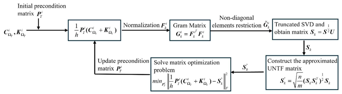
where g_ij represents the non-diagonal elements of the Gram matrix in the ith row and the jth column. Then, the matrix ${\mathit{P}}_T^i({\displaystyle \frac{1}{h}}{\mathit{C}}_{{\mathbf{\Omega }}_T}^i+{\mathit{K}}_{{\mathbf{\Omega }}_T}^i)\in {\mathit{R}}^{m\times n}$ would be approximated to the UNTF. For each flexible body thermal part, the preconditioned matrix is obtained using the flowchart shown in Figure 1. Specifically, it can be described as the following steps:

Step 1: The matrix ${\mathit{P}}_T^i({\displaystyle \frac{1}{h}}{\mathit{C}}_{{\mathbf{\Omega }}_T}^i+{\mathit{K}}_{{\mathbf{\Omega }}_T}^i)$ is normalized to get a matrix ${\mathit{F}}_k^i$, where k indicates the current iteration number.

Step 2: Construct the Gram matrix by ${\mathit{G}}_k^i={\mathit{F}}_k^{i^T}{\mathit{F}}_k^i$. Then, the non-diagonal elements value of this matrix are restricted by formula (29). The matrix after restricting is marked as ${\tilde{\mathit{G}}}_k^i$.

Step 3: To make the rank of the Gram matrix equal to m, the truncated SVD is applied to approximate ${\tilde{\mathit{G}}}_k^i$, and obtains the approximated matrix $\stackrel{⌣}{\mathit{G}}$. Then, calculate the matrix ${\mathit{S}}_{\mathit{k}}={\mathit{S}}^{{\displaystyle \frac{1}{2}}}\mathit{U}$ by utilizing the singular value matrix, which $\stackrel{⌣}{\mathit{G}}={\mathit{S}}_{\mathit{k}}^{\mathit{T}}{\mathit{S}}_{\mathit{k}}$.

Step 4: Construct the matrix to approximate the UNTF by ${\mathit{S}}_{\mathit{k}}^{\prime }=\sqrt{{\displaystyle \frac{n}{m}}}{({\mathit{S}}_{\mathit{k}}{\mathit{S}}_{\mathit{k}}^{\mathit{T}})}^{{\displaystyle \frac{1}{2}}}{\mathit{S}}_{\mathit{k}}$.

Step 5: To make the thermal matrix approximate the UNTF by a precondition matrix ${\mathit{P}}_T^i$, the matrix minimization problem ${\mathit{min}}_{{\mathit{P}}_{\mathit{T}}^{\mathit{i}}}{‖{\mathit{P}}_T^i({\displaystyle \frac{1}{h}}{\mathit{C}}_{{\mathbf{\Omega }}_T}^i+{\mathit{K}}_{{\mathbf{\Omega }}_T}^i)-{\mathit{S}}_{\mathit{k}}^{\prime }‖}_F^2$ is constructed. By solving the problem, the precondition matrix ${\mathit{P}}_{T_{\mathit{k}}}^i$ can be obtained.

Step 6: If $k\le \mathit{iter}$, then set $k=k+1$ and set back to Step 1. Otherwise, exit the constructor and output the preconditioned matrix ${\mathit{P}}_{T_{\mathit{k}}}^i$.

For solving the matrix minimization problem in Step 5, let $\mathit{B}={\mathit{P}}_T^i({\displaystyle \frac{1}{h}}{\mathit{C}}_{{\mathbf{\Omega }}_T}^i+{\mathit{K}}_{{\mathbf{\Omega }}_T}^i)$. Then, take the derivative of the norm with respect to P to equal the zero matrix, which can be expressed as:

$${\displaystyle \frac{\partial {‖\mathit{P}\mathit{B}-{\mathit{S}}_{\mathit{k}}^{\prime }‖}_F^2}{\partial \mathit{P}}}=\mathbf{0}$$

(30)

According to the matrix derivation law [47], the following matrix equations can be obtained:

$$\mathit{P}\mathit{B}={\mathit{S}}_{\mathit{k}}^{\prime }\iff \mathit{P}={\mathit{S}}_{\mathit{k}}^{\prime }{\left(\mathit{B}{\mathit{B}}^{\mathit{T}}\right)}^{-1}$$

(31)

So, the solution of the matrix minimization problem in Step 5 can be obtained by Equation (31).

3.3. Summary of Sparse Model Order Reduction Method for Thermomechanical Dynamic System

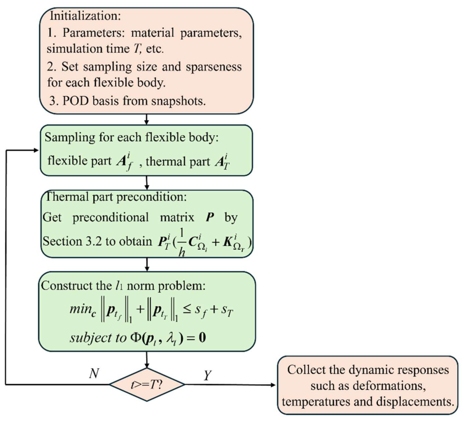
The previous sections detailed the sparse model reduction method for the thermomechanical coupling dynamic system. The analysis flowchart is depicted in Figure 2. The key contributions of this paper are highlighted in green areas. The flowchart outlines the proposed method for analyzing the thermomechanical coupling system, broken into five steps.

Step 1: Initial setup includes defining material parameters, such as Young’s modulus and specific heat, as well as simulation parameters, such as sampling size, sparseness, and duration. Subsequently, the POD basis is calculated from the collected data points using Equation (9). The mass, stiffness, and other constants are determined via inertia shape integration.

Step 2: The Latin Hypercube sampling technique is employed to establish the indices for the equations. Based on these indices, the necessary sampling matrices, including the mass, stiffness, and capacitance matrices, are calculated, eliminating the need to use the entire set.

Step 3: The preconditioning matrix for the thermal Jacobian of the flexible body is obtained using the procedures outlined in Section 3.2.

Step 4: The POD coefficients l₁ norm problem, constrained by the sampling Equation (25) at each time step, is constructed. By using the Greedy-Gauss-Newton method to solve the problem, the coefficients pt and the Lagrange multiplier at each time step are obtained. Then, the deformation, temperature, position, etc., can be collected.

Step 5: If the current time t is less than the simulation time T, go back to Step 2 for the next time step analysis. Otherwise, the simulation is finished.

The key mathematical difference between the proposed method and conventional projection-based reduced-order models (e.g., POD-Galerkin and hyper-reduction) lies in how the governing equations are treated. Conventional methods first project the full-order system onto a low-dimensional subspace via Galerkin projection, yielding a reduced system of dimension $\mathit{r}$ (the number of retained POD modes):

$${\mathit{U}}^T\mathbf{\Phi }(\mathit{U}\mathit{p})=\mathbf{0},\mathit{p}\in {\mathit{R}}^r$$

(32)

where $\mathbf{\Phi }(·)$ is the residual of the full-order equations. The computational cost of this reduced system, however, remains dependent on the full-order dimension $\mathit{N}$ when evaluating nonlinear terms.

In contrast, the proposed method does not perform Galerkin projection. Instead, it directly samples $\mathit{m}\ll \mathit{N}$ equations from the full-order residual and solves for the sparse coefficients $\mathit{p}\in {\mathit{R}}^N$ via l₁ optimization:

$$\mathit{m}\mathit{i}\mathit{n}\parallel \mathit{p}{\parallel }_{1}s.t.\mathit{P}\mathbf{\Phi }(\mathit{U}\mathit{p})=\mathbf{0},\mathit{P}\in {\mathit{R}}^{m\times N}$$

(33)

where $\mathit{P}$ is a sampling matrix selecting $\mathit{m}$ rows of the residual. The reduction is achieved through sparsity: only a few components of $\mathit{p}$ are active at each time step, and these are adaptively selected online. This avoids both the projection error of Galerkin methods and the offline-fixed interpolation points of hyper-reduction techniques such as DEIM.

In the POD-Galerkin method, the number of retained POD bases is determined by a fixed energy criterion during the offline stage, and all retained bases are used for projection. In contrast, in the proposed method, the basis size is chosen to ensure that the state variables can be sparsely represented on the selected basis; only a sparse subset of the retained bases is active online via the l₁ optimization at each time step. The framework itself is not restricted to POD and can adopt any basis, including overcomplete ones, provided that a sparse representation exists for the given system.

4. Numerical Results

This section presents three numerical examples that illustrate the practicality of the proposed method for the thermomechanical coupling system. The simulations were conducted using MATLAB 2019b on a system equipped with an Intel Core i7-10700F processor running at 2.9 GHz and 16 GB of RAM.

Three examples are selected to validate the proposed method progressively. The first example (a double pendulum) demonstrates the method fundamental accuracy in a basic thermomechanical configuration, where thermal radiation introduces a moderate coupling effect. The second example (slider-plate system) introduces frictional heat generation, validating the method ability to handle contact-induced nonlinearities and moving thermal sources. The third example (brake disk) represents a more challenging engineering application, where high thermal gradients and strong frictional heating test the robustness and stability of the method. Together, these examples cover different sources of thermomechanical coupling (radiation, friction, and high-gradient heating) and progressively increase in complexity, providing a comprehensive validation of the proposed framework.

4.1. Example 1: A Double Pendulum

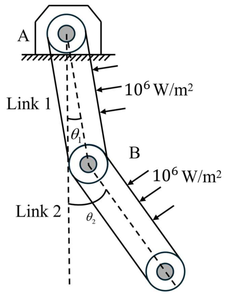
The double pendulum system is presented as the first example, and its structure is shown in Figure 3. In Figure 3, the double pendulum is constructed of two links. Link 1 is fixed to the ground through the revolute joint A with a diameter of 0.085 m. Link 2 is connected to Link 1 by the revolute joint B. In addition, the shape of Link 2 is the same as that of Link 1. The two linkages are modeled as flexible bodies and meshed with 1280 low-order triangular elements. The thickness is 0.03 m. The reference and initial temperature are set to be 293.15 K. The initial angles of the two links are set to 0° and 5°, respectively. In this example, the upper boundary of the two linkages is subjected to 1 $\times$ 10⁶ W/m² radiation flux, while the other boundaries are insulated. In addition, the sparsity of the deformation and thermal field of the two linkages is set to 80 and 20, respectively. The simulation time and step size are set to 4 s and 1 $\times$ 10⁻³ s. The material properties of the two linkages are shown in

Table 1. Material properties for the double pendulum.

Properties	Link 1 and Link 2
Specific heat (J/(kg∙K))	475
Heat conduction (W/(m∙K))	44.5
Thermal expansion (1/K)	2 ${\times 10}^{-5}$
Density (kg/m3)	1000
Young’s modulus (Pa)	7 ${\times 10}^{10}$
Poisson’s ratio	0.3

.

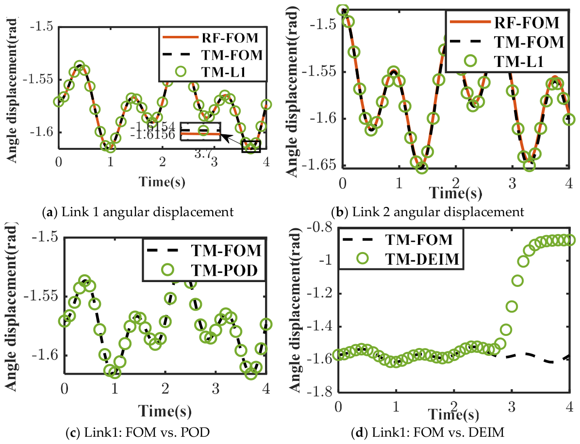
In this example, the rigid-flexible and thermomechanical coupling systems are simulated. Since the full order method (FOM) represents the original high-fidelity dynamics and is widely used as the benchmark for validating reduced-order models, FOM and the proposed l₁ norm method (L1) are utilized to calculate the dynamic responses of the thermomechanical case. In addition, the POD and POD-DEIM methods are utilized compared with the L1 norm method. POD and POD-DEIM use the same snapshot data and share the same number of POD bases for state reduction with the L1 method. For the DEIM, an additional POD basis is constructed for the nonlinear term. The number of its retained modes and the corresponding interpolation points are determined by the energy criterion 0.9999. Specifically, for Link 1, the nonlinear term POD bases are 1277 for the elastic part and 13 for the thermal part, with interpolation points 1277 and 13. For Link 2, the corresponding values are 955 and 13. Firstly, the angular displacements are shown in Figure 4. As shown in Figure 4a,b, small deviations are observed between the rigid-flexible (RF-FOM) and thermomechanical (TF-FOM) models for Link 1, while the deviation for Link 2 increases over time, indicating that the thermal load significantly influences the dynamic characteristics of the double pendulum. The angular displacements computed by the proposed L1 method agree almost perfectly with the TM-FOM throughout the entire simulation. The POD method also yields results consistent with TM-FOM, showing only minor discrepancies. For the DEIM, the angular displacements match TF-FOM well during the initial stage; however, as time progresses, the error gradually accumulates, leading to a noticeable divergence after approximately 2.4 s. This behavior highlights the limitation of DEIM in capturing long-term thermomechanical coupling dynamics.

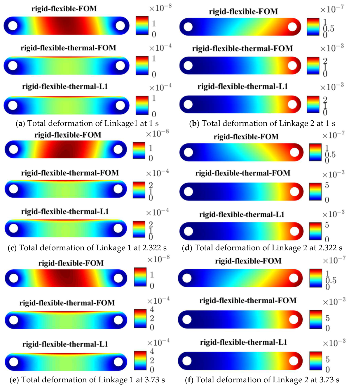
To analyze the deformation distribution of flexible bodies under thermal loading, the total deformation of the linkages at 1 s, 2.332 s, and 3.73 s is shown in Figure 5. As shown in Figure 5, the deformation of the linkages increases by approximately 4 orders of magnitude due to the radiation flux compared with the rigid-flexible case. The maximum deformation of Link 1 is on the upper boundary, where the radiation flux is applied. In addition, the deformation amplitude increases gradually over time, while the rigid-flexible model is almost unchanged. In Figure 5, the thermomechanical deformation calculated by the L1 norm method is nearly identical to that of FOM.

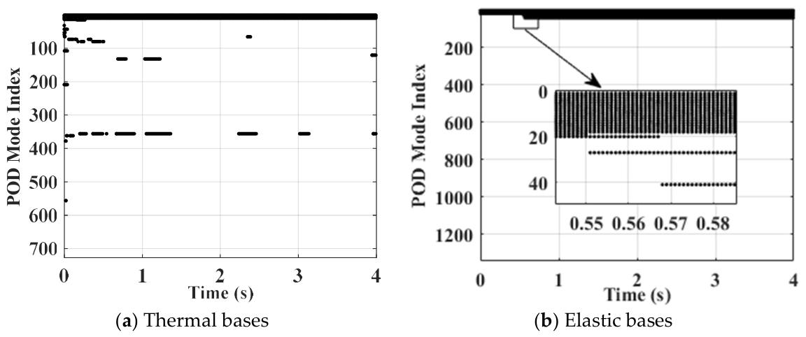
To verify that the adaptive basis selection remains effective after replacing modal bases with POD bases in the thermomechanical setting, Figure 6 compares the evolution of the selected thermal and elastic POD coefficients for Link 1. In both panels, a black dot indicates that the coefficient is non-zero at that time step (activated by the L1 method), while white regions denote zero coefficients. Two observations are worth highlighting. First, the selected elastic bases remain nearly unchanged throughout the simulation, indicating that a persistent set of modes well represents the deformation. Second, the active thermal bases vary over time, indicating that the L1 method adaptively reselects the POD modes as the thermomechanical state evolves.

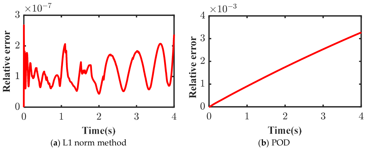
To quantitatively evaluate the accuracy of the L1 norm method and compare it with the traditional projection-based POD approach, Figure 7 presents the relative error curves of both methods with respect to FOM. The following formula calculates the relative errors:

$$e_r={\displaystyle \frac{{‖{\mathit{q}}_{\mathit{FOM}}(t)-{\mathit{q}}_{L1}(t)‖}_2}{{‖{\mathit{q}}_{\mathit{FOM}}(t)‖}_2}}$$

(34)

where q includes all coordinates jointly. As illustrated in Figure 7, a monotonic increase in the POD relative error is observed throughout the 4 s simulation. This trend can be attributed to the construction of the POD basis from a fixed set of modes. As the system evolves, its instantaneous configuration gradually departs from the subspace spanned by these modes, thereby leading to the progressive accumulation of projection and truncation errors. In essence, the POD subspace becomes progressively less representative of the evolving system dynamics. By contrast, the L1 norm method maintains a consistently low error level (maximum error is 2.68 $\times$ 10⁻⁷), indicating that its sparse representation framework is inherently more tolerant to slow, continuous shifts in the motion characteristics of this example.

Additionally, the computational efficiency of the FOM, L1-norm method, and POD method is shown in

Table 2. The efficiency of the FOM and L1 norm method (unit s).

Approach	Matrix Operations	Update (Mass, Jacobian, Residual)	Overall Duration
FOM	4686	4059	8745
POD	241	3201	3442
L1 norm	1236	378	1823

. In Table 2, the computation time of the L1 norm method and the POD method is faster than that of FOM. Computation time accounts for approximately 21% and 39% of that of the FOM. In addition, the L1 norm method achieves the highest computational efficiency during the updates of the mass matrix, Jacobian matrix, and nonlinear functions, yielding an improvement of approximately 90%. In contrast, for the POD method, these update operations account for nearly 93% of the total computational cost. This efficiency advantage arises because the L1 norm method does not require assembling or operating on the full system matrices; instead, only the rows corresponding to the selected sampling indices are evaluated. Consequently, the update process becomes significantly faster.

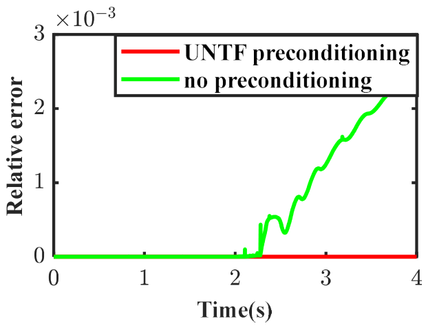
Lastly, Figure 8 presents the evolution of the relative error for the L1 norm method with (red curve) and without (green curve) the proposed UNTF preconditioning. A clear numerical distinction is observed between the two configurations. In the absence of preconditioning, the relative error remains small during the initial stage of the simulation; however, after approximately 2 s, it begins to grow steadily and eventually reaches the order of 10⁻³. This progressive error amplification reflects the numerical instability caused by the strong correlation, which leads to accumulated residuals and degraded convergence of the nonlinear solver, ultimately resulting in a diverging solution trajectory. In contrast, the UNTF preconditioned formulation maintains a consistently low, nearly constant relative error throughout the entire simulation horizon. The stable error profile demonstrates that the proposed preconditioning effectively decorrelates the Jacobian rows and suppresses the propagation of numerical disturbances. Notably, during the period in which the non-preconditioned solver exhibits rapidly increasing error (2–4 s), the preconditioned solver remains fully stable, confirming its robustness in handling the thermomechanical coupling dynamics.

To investigate the influence of the sparsity parameters on the accuracy of the proposed method, a sensitivity study is conducted on the double pendulum example.

Table 3. Sensitivity of accuracy and efficiency to elastic sparsity.

Elastic Sparsity	Max Relative Error	Computational Time
20	2.19 $\times$ 10−4	1990
40	4.81 $\times$ 10−7	2042
60	3.81 $\times$ 10−7	1823

summarizes the max relative errors and CPU times for different elastic sparsity values for Link 1 and Link 2. A similar sensitivity study is conducted for thermal sparsity, and the results are shown in

Table 4. Sensitivity of accuracy and efficiency to thermal sparsity.

Thermal Sparsity	Max Relative Error	Computational Time
5	0.0013	2107
10	5.11 $\times$ 10−6	2054
15	4.21 $\times$ 10−7	1989

. As shown in Table 3 and Table 4, the accuracy degrades significantly when the sparsity parameters are too small. For the elastic sparsity, increasing from 20 to 60 reduces the error from 2.19 $\times$ 10⁻⁴ to 3.81 $\times$ 10⁻⁷. For the thermal sparsity, increasing from 5 to 15 similarly reduces the error from 0.0013 to 4.21 $\times$ 10⁻⁷. In both cases, the error reaches the 10⁻⁷ level when elastic sparsity and thermal sparsity are set to more than 40 and 15, respectively. The computational time remains approximately constant at around 2000 s across all cases, indicating that the efficiency of the method is not sensitive to the choice of sparsity parameters.

4.2. Example 2: A Slider Plate

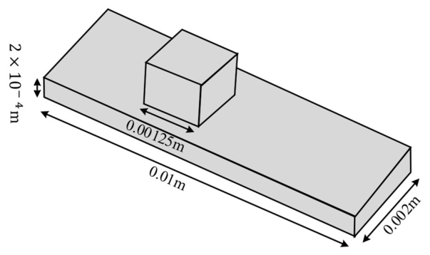
To further demonstrate the feasibility of the proposed method, the dynamic characteristics of frictional heat generation during the movement of the slider on the plate are analyzed. Then, the temperature distribution is compared with the results calculated in [48]. The geometric model of this example is shown in Figure 9. The slider and plate are modeled as flexible bodies, divided into 1336 and 2034 low-order triangular elements, respectively. In this model, the plate is fixed to the ground, and the slider starts at the far left of the plate and moves to the right at 1 m/s. In addition, a 10 MPa pressure is applied to the upper surface of the slider. Since the deformation of the flexible bodies is assumed small in this example, the rigid-body model can be established first to reduce the computational burden of the contact model. The contact force is calculated by the polygonal contact model [49]. Then, the contact elements and forces are collected and imported into the thermomechanical coupling model. The friction coefficient between the slider and the plate is set to be 0.2, while the contact stiffness, damping coefficient, penetration threshold, and velocity critical value of friction are set to be 6.11 $\times$ 10¹³ N/m, 6.1214 $\times$10⁴ Ns/m, 1 $\times$ 10⁻⁹ m, and 0.05 m/s, respectively. The dynamic response of the thermomechanical coupling model is obtained by the proposed L1 norm method. The sample size and sparsity of the flexible part of the slider are set to be 200 and 80, respectively, while the thermal field part is set to be 400 and 100, respectively. The total simulation time and time step are 3.75 $\times$ 10⁻³ s and 3.75 $\times$ 10⁻⁶. The material properties of the slider and plate correspond to the initial temperature condition. The relative parameters are listed in

Table 5. The material parameters of the slider plate system.

Properties	Slider/Plate
Young’s modulus	70.006 GP
Poisson’s ratio	0.3
Density	2700 kg/m3
Thermal expansion	23.8 $\times$ 10−6 °C−1
Heat transfer coefficient	150 Ns/°C

.

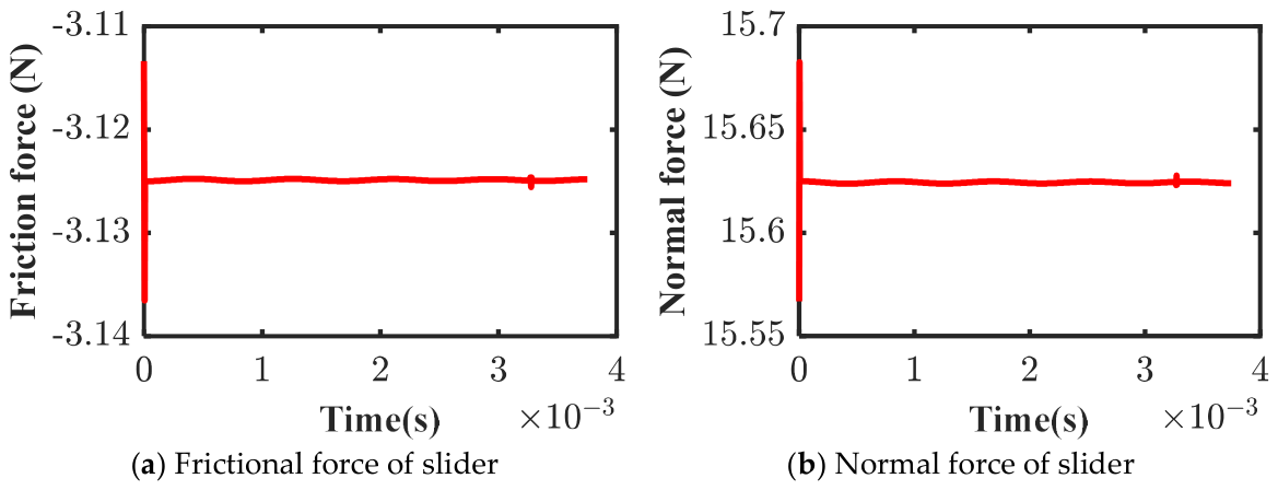
Due to the applied pressure and the slider’s self-weight, frictional heat can be generated between the slider and the plate. The total frictional force and the normal pressure of the slider are calculated using the polygon contact model shown in Figure 10. In Figure 10, fluctuations in frictional and normal forces occurred, resulting from the slider falling from the upper boundary of the plate to the height of the penetration at the beginning of the contact. The average of frictional and normal forces is 3.115 N and 15.625 N.

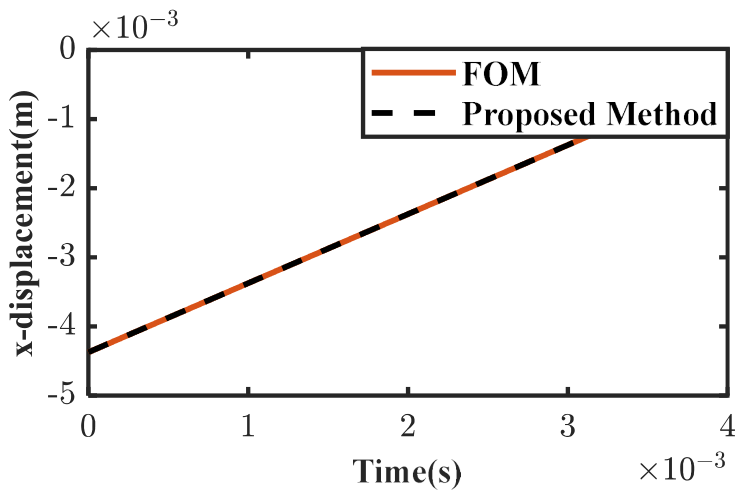
After importing the contact forces into the thermomechanical coupling model, the displacement of the slider along the x-axis was calculated, as shown in Figure 11. In Figure 11, the displacement curve obtained by the L1 norm method is nearly identical to that of FOM as the slider moves to the right at a constant speed. The close agreement confirms that the proposed method accurately captures the rigid motion, as the rigid coordinates are not reduced.

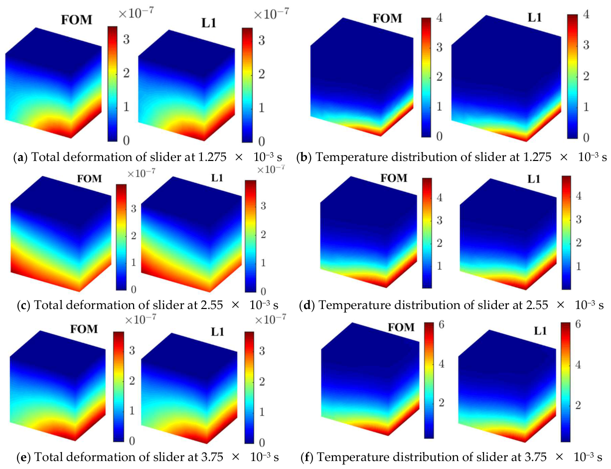
The total deformation distribution and temperature distribution of the slider at 1.275 $\times$ 10⁻³ s, 2.55 $\times$ 10⁻³ s, and 3.75 $\times$ 10⁻³ s are shown in Figure 12. In the deformation distribution, the deformation amplitude increases slightly during sliding. As shown in the temperature distribution, the slider temperature gradually increases as it moves. At the last moment, the maximum temperature calculated by the FOM and L1 norm methods is 6.1380 °C and 6.1382 °C, respectively, while the maximum temperature calculated in [48] is about 6.10 °C. In addition, regardless of the deformation or temperature distribution, the results from the L1 norm method are nearly identical to those from FOM. The above analysis shows that the L1 norm method is suitable for analyzing the dynamic response of the thermomechanical coupling model.

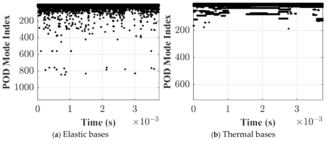
Similarly, Figure 13 illustrates the adaptive basis selection for the plate. Both the elastic and thermal bases vary over time, reflecting the continuously changing contact condition and frictional heat generation as the slider moves along the plate. This indicates that the L1 norm method adaptively reselects the POD modes in response to the evolving thermomechanical state, without relying on a pre-determined offline subspace.

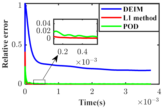
To compare the accuracy of the L1 method with POD and POD-DEIM, the relative errors of the three methods with respect to FOM are presented in Figure 14. For a fair comparison, all methods share the same snapshot data and use the same number of state POD modes. For the DEIM, the nonlinear-term POD bases and interpolation points are also determined by the same energy criterion of 0.9999. Specifically, for the slider, the DEIM bases are 75 and 98 for the elastic and thermal parts, respectively. For the plate, the corresponding values are 6 and 9. As shown in Figure 14, DEIM, the L1 method, and POD experience pronounced errors during the initial transient stage, primarily due to the high-frequency responses introduced by contact activation in the slider-plate friction system. At this stage, the relative errors of the L1 method, POD, and DEIM reach approximately 0.4, 0.2, and 1.0, respectively, with DEIM exhibiting the largest deviation. Once the system transitions into the steady sliding regime, the dynamics become dominated by simple motion patterns. Under these conditions, the POD basis captures the predominant sliding characteristics sufficiently well, and its error stabilizes at around 4 $\times$ 10⁻³. The L1 method achieves the highest accuracy among the three, with its relative error converging to approximately 7 $\times$ 10⁻⁴. In contrast, DEIM fails to recover from the initial transient error and converges to a relatively high steady-state error of about 0.2, indicating that the fixed interpolation points selected offline are not well-suited for the contact-induced nonlinearities in this system.

Table 6. The computational efficiency of FOM and L1 norm method (unit s).

Approach	Matrix Operations	Update (Mass, Jacobian, Residual)	Overall Duration
FOM	240	405	647
POD	175	396	571
L1 norm	186	204	395

summarizes the computational efficiency of the FOM, L1, and POD methods for the present numerical example. Both the L1 method and the POD method achieve significant reductions in computation time compared with FOM, requiring approximately 60% and 88% of FOM, respectively. Notably, the L1 method demonstrates the highest efficiency during updates to the mass matrix, Jacobian matrix, and nonlinear terms, achieving roughly a 50% improvement. In contrast, these update operations account for nearly 69% of the computational cost of the POD method.

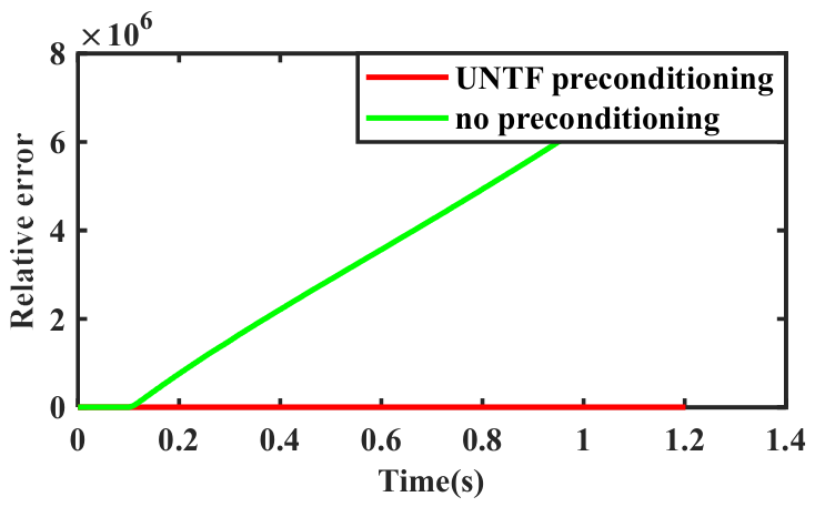
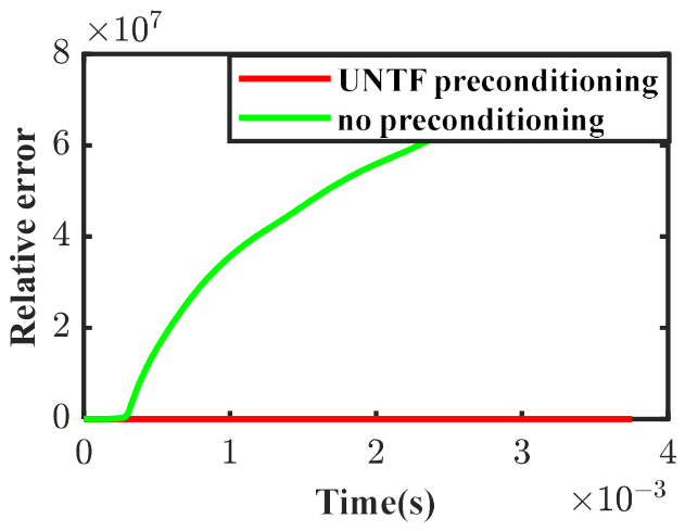
Figure 15 illustrates the relative error of the L1 method with and without UNTF preconditioning. The results show that preconditioning effectively maintains the relative error at a stable level, whereas without preconditioning, the error grows rapidly to the order of 10⁷. This highlights that UNTF preconditioning substantially improves the numerical stability and robustness of the L1 norm method.

Sensitivity studies are also conducted on the slider-plate example for the elastic sparsity of both the slider and the plate. The results are summarized in

Table 7. Sensitivity of accuracy and efficiency to elastic sparsity for slider.

Elastic Sparsity	Max Relative Error	Computational Time
20	0.423	404
40	0.397	397
60	0.402	401

and

Table 8. Sensitivity of accuracy and efficiency to elastic sparsity for plate.

Elastic Sparsity	Max Relative Error	Computational Time
10	2.902	362
20	1.523	345
50	0.738	381

. For the slider, varying sparsity from 20 to 60 yields max relative errors that remain approximately constant around 0.4, indicating that the slider elastic field is relatively insensitive to the sparsity parameter in this range. For the plate, increasing sparsity from 10 to 50 reduces the relative error from 2.902 to 0.738, suggesting that the plate elastic field requires a sufficient sparsity level to achieve reasonable accuracy. The computational time remains stable across all cases (approximately 340–404 s).

4.3. Example 3: A Brake Disk

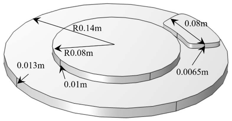
The geometric model of the brake disk is shown in Figure 16 and consists of a disk and a pad. In this model, the pad moves only on the z-axis while the disk rotates around the z-axis. In Figure 16, the radius of the disk is 0.14 m, while the thickness of the disk and pad is 0.013 m and 0.0065 m. In this example, the car is moving forward at 60 km/h, and the tire radius is 0.25 m. Then, the disk rotates at 66.67 rad/s. In addition, an 18 kN force is applied to the top surface of the pad, which would bring it into contact with the disk and generate a frictional force. The friction coefficient is set to 0.7. The material properties of the disk and pad are shown in

Table 9. The material properties of the disk and pad.

Properties	Disk	Pad
Specific heat (J/(kg∙K))	475	935
Heat conduction (W/(m∙K))	44.5	8.7
Thermal expansion (1/K)	12.3 $\times$ 10−6	60 $\times$ 10−6
Density (kg/m3)	7850	2000
Young’s modulus (Pa)	200 $\times$ 109	2000
Poisson’s ratio	0.3	0.3

. The disk and pad are treated as flexible bodies, which were divided into 10,345 and 902 low-order tetrahedra, respectively, and the simulation time and time step are set to 1.2 s and 110-3 s, respectively. When the L1 norm method is applied, the sampling number and sparsity of the elastic and thermal field of the disk are set to (1200, 400) and (200, 50), while the pad sampling number and sparsity are set to (320, 140) and (150, 50).

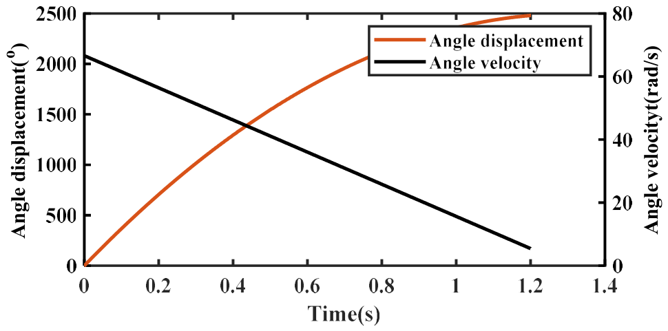
Similar to Example 2, the polygon contact model is used to model the frictional contact between the disk and pad. The contact force is then imported into the thermomechanical system for dynamic analysis. Applying the contact model, the angle displacement and velocity are shown in Figure 17. In Figure 17, the angular velocity decreases linearly, and the angular displacement increases gradually.

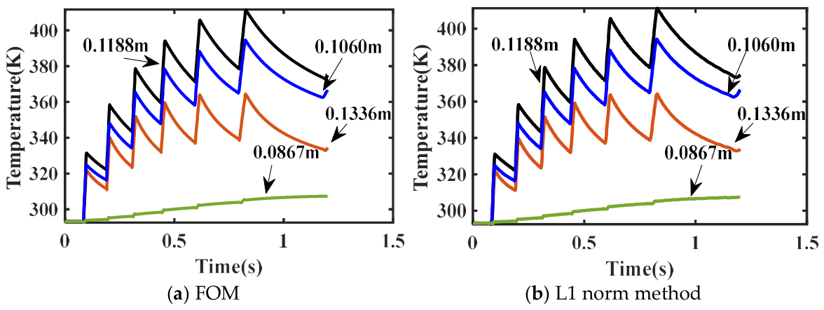
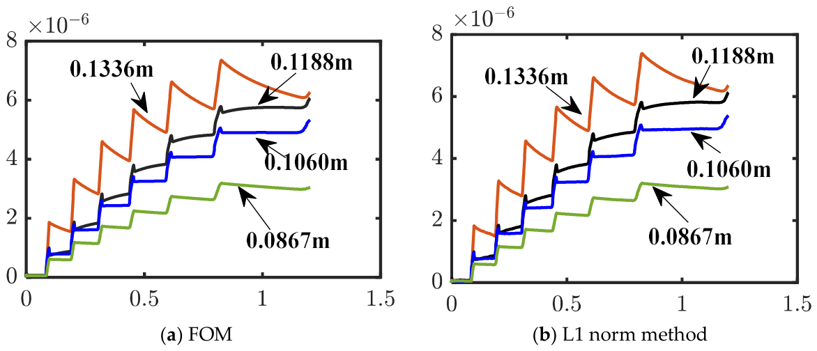
Due to friction, heat flux flows to the disk and pad, and the temperature distribution of the brake disk system changes. The temperature curves of four nodes on the disk surface, which are calculated by the FOM and L1 norm methods, are shown in Figure 18. In Figure 18, the solid black line represents the temperature curve of nodes 0.1188 m away from the rotation axis of the disk, while blue, red, and green lines represent the temperatures of nodes 0.1060 m, 1.336 m, and 0.0867 m away from the rotation axis of the disk, respectively. As shown in Figure 18, the temperature variation appears to be extremely sharp. During each braking cycle, the frictional heat flux is applied over a very narrow contact area and over a short time interval, leading to an intense, highly localized heat input. As a result, steep thermal gradients are formed in the radial direction. Once the brake force is released, the heat rapidly diffuses into the surrounding material and dissipates through convection, causing a rapid temperature drop. This combination of concentrated heat generation and fast subsequent cooling produces spike-like temperature profiles. A similar phenomenon has also been reported in [50,51]. Sharp gradients can challenge the L1-norm method. Since the sparse bases are used to approximate the temperature and deformation fields, insufficient sparsity of these fields with respect to the chosen bases can result in significant approximation errors. To reduce such errors, the number of basis vectors may be increased, or alternative sparse bases with stronger representational capacity may be employed. In addition, nodes closer to the contact area are higher, while nodes farther away are cooler. Comparing the results of (a) and (b) in Figure 18, the temperature curves calculated by the L1 norm method are consistent with the FOM.

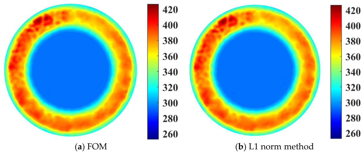
The disk temperature distribution at 1.2 s is shown in Figure 19. As shown in Figure 19, the maximum temperature on the disk surface calculated by FOM is 426.7 K. The maximum temperature calculated in [50] is 432 K. The model error is about 1.2% compared with [50]. In Figure 19, the temperature on the contact area is significantly higher than in the non-contact area, and the farther away from the contact area, the lower the temperature. Additionally, the temperature distribution calculated by the L1 norm method is consistent with FOM.

The total deformation of the four nodes is shown in Figure 20. As shown in Figure 20, the nodal deformation on the disk surface gradually decreased from the outer edge to the inner edge, and the maximum deformation is 7.23 $\times$ 10⁻⁶ m. In addition, the results calculated using the L1 norm method are consistent with FOM.

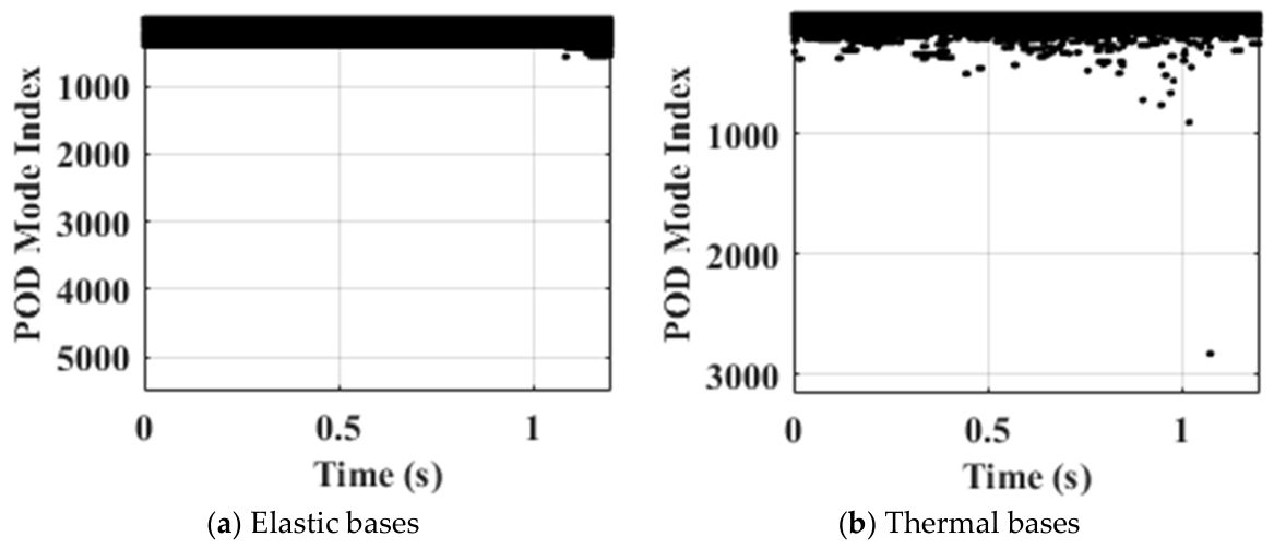
Figure 21 illustrates the adaptive basis selection for the disk. The elastic bases remain relatively stable throughout the simulation, indicating that a persistent set of modes well captures the deformation. In contrast, the thermal bases show clear temporal variation, with the active modes changing as heat flux is generated and dissipated during braking. This is consistent with the highly transient nature of the thermal field in the brake disk, where the temperature distribution evolves rapidly due to localized frictional heating and subsequent cooling. The results confirm that the L1 method adaptively reselects the POD modes in response to changes in the thermomechanical state.

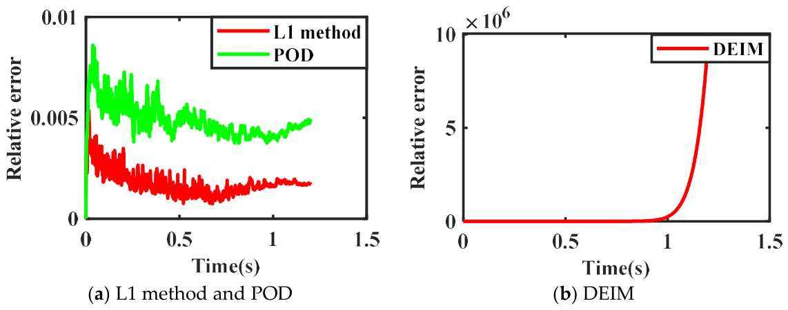
To compare the accuracy of the L1 method with POD and POD-DEIM, the relative errors of the three methods with respect to FOM are shown in Figure 22. For a fair comparison, all methods share the same snapshot data and use the same number of state POD modes. For the DEIM, the nonlinear-term POD bases and interpolation points are also determined by the energy criterion 0.9999. Specifically, for the disk, the DEIM bases are 1199 and 1194 for the elastic and thermal parts, respectively. For the pad, the corresponding values are 582 and 251. As shown in Figure 22. The L1 method and POD exhibit generally similar error trends throughout the simulation, with L1 maintaining a slightly lower error level than POD. In contrast, the DEIM shows a sharp increase in error starting at approximately 1 s, with the relative error rapidly rising to the order of 10⁶. This divergence indicates that the offline-fixed interpolation points selected by DEIM fail to capture the rapidly evolving thermal and frictional fields in the brake disk, leading to a breakdown of the reduced-order model. The results highlight the robustness of the L1 method online adaptive sampling strategy in handling nonlinear thermomechanical coupling, whereas DEIM is vulnerable to instability when the system dynamics deviate from the offline training data.

Table 10. Computation efficiency of FOM and l₁ norm method (Unit s).

Approach	Matrix Operations	Update (Mass, Jacobian, Residual)	Overall Duration
FOM	656	4523	5182
POD	599	3783	4382
L1 norm	322	2241	2566

reports on the computational efficiency of the FOM, L1 norm method, and POD method for this case study. Both reduced-order approaches exhibit notable time savings relative to FOM, with the L1 norm method and POD method requiring approximately 49% and 84% of the full-order computational cost, respectively. The L1 norm method shows the greatest advantage during the updates of the mass matrix, Jacobian matrix, and nonlinear terms, achieving an efficiency improvement of roughly 50%. In comparison, these update procedures remain the dominant contributors to the computational cost of the POD method, accounting for nearly 86% of its total runtime.

Figure 23 presents the relative error of the L1-norm method for the current example, comparing results with and without UNTF preconditioning. The preconditioned formulation maintains a consistently low error level throughout the simulation, whereas the non-preconditioned case exhibits a rapid increase in error, eventually reaching the order of 10⁶. This demonstrates that incorporating UNTF preconditioning significantly enhances the numerical stability and robustness of the L1-based reduction procedure for this example.

Sensitivity studies are also conducted on the brake disk example for both elastic and thermal sparsity. The results are summarized in

Table 11. Sensitivity of accuracy and efficiency to elastic sparsity for disk.

Elastic Sparsity	Max Relative Error	Computational Time
20	0.0144	2347
50	0.0137	2238
100	0.0124	2526

and

Table 12. Sensitivity of accuracy and efficiency to thermal sparsity for disk.

Thermal Sparsity	Max Relative Error	Computational Time
5	0.0735	2359
10	0.0268	2471
30	0.0135	2359

. For the elastic sparsity, varying from 20 to 100 yields relative errors that remain approximately constant around 0.012–0.014, indicating that the elastic field of the disk is largely insensitive to the sparsity parameter. For the thermal sparsity, increasing from 5 to 30 reduces the relative error from 0.0735 to 0.0135, showing a clear improvement. However, compared with the double pendulum case, the improvement is more limited, and the error level remains higher. The computational time remains stable across all cases.

5. Conclusions

This paper proposes a projection-free sparse model reduction framework for thermomechanical coupling dynamics of flexible multibody systems, where the full-order equations are directly sampled online, and the reduced coefficients are recovered via ${\mathit{l}}_1$ norm optimization without Galerkin projection. The framework extends the projection-free paradigm to thermomechanical coupling by replacing modal bases with data-driven POD bases to capture the time-varying thermal subspace and by introducing UNTF preconditioning to ensure stable recovery under thermal-mechanical coupling. These developments enable, for the first time, the application of the projection-free sparse model reduction paradigm to thermomechanical coupling problems.

The numerical results demonstrate the effectiveness of the proposed method across three representative examples. In the double pendulum case, the L1 method achieves the highest accuracy, with relative errors on the order of 10⁻⁷. For the slider-plate and brake disk systems, the L1 method maintains good accuracy, with stable error levels comparable to or slightly better than those of POD-Galerkin, while showing significantly greater robustness than DEIM. Computational efficiency is consistently improved, with total simulation time reduced by more than 40% across all three examples. The UNTF preconditioner is shown to be essential for numerical stability, as the un-preconditioned solver leads to rapidly growing errors.

Sensitivity studies on the sparsity parameters indicate that the required sparsity level depends on the POD basis ability to represent the system dynamics. For systems with dominant low-order dynamics (e.g., the double pendulum), moderate sparsity is sufficient to achieve high accuracy. For systems with strong localized features or complex nonlinearities (e.g., the slider-plate and brake disk), increasing the sparsity yields diminishing returns due to the inherent limitation of global POD bases in capturing localized phenomena. Computational time remains stable across all cases, confirming that efficiency is not sensitive to the choice of sparsity parameters. These findings suggest that the sparsity parameters should be chosen based on a problem-dependent threshold, above which accuracy saturates, rather than relying on a universal fixed value.

The theoretical foundation of the proposed method relies on the well-established restricted isometry property (RIP) in compressed sensing theory. While a new theoretical proof of RIP for the specific thermomechanical system is not provided in this paper, the numerical results across three representative—covering thermal radiation, frictional heat generation, and transient high-gradient heating—provide strong empirical evidence of the method reliability under various thermomechanical conditions.

Despite these advantages, the proposed method has certain limitations when applied to systems with discontinuous contact forces, potentially yielding low-precision dynamic results. This limitation arises not only from the difficulty of accurately capturing rapidly changing contact characteristics through random sampling of the dynamic equations, but also from the insufficient sparsity of the corresponding temperature or deformation fields under the chosen sparse bases. When the true field cannot be sparsely represented, the l₁-based reconstruction becomes less effective. Future research should therefore focus on optimizing the sampling strategy and improving the sparse representation framework to better capture the dynamic characteristics in such cases.

References

1. Wolff, A.; Kukulski, J. Numerical and experimental analysis of the heat transfer process in a railway disc brake tested on a dynamometer stand. Open Eng. 2023, 13, 20220466. [Google Scholar] [CrossRef]
2. Grzes, P.; Kuciej, M. Coupled thermomechanical fe model of a railway disc brake for friction material wear calculations. Wear 2023, 530–531, 205049. [Google Scholar] [CrossRef]
3. Li, Y.; Zhang, Y.; Zhao, Y.; Shi, X. Thermal-mechanical coupling calculation method for deformation error of motorized spindle of machine tool. Eng. Fail. Anal. 2021, 128, 105597. [Google Scholar] [CrossRef]
4. Aggogeri, F.; Merlo, A.; Pellegrini, N. Modeling the thermo-mechanical deformations of machine tool structures in cfrp material adopting data-driven prediction schemes. Mechatronics 2020, 71, 102436. [Google Scholar] [CrossRef]
5. Zhang, J.; Zheng, J. Thermal and mechanical stress analysis in aircraft hybrid panels with multi-bolt joints. Materials 2024, 17, 1872. [Google Scholar] [CrossRef] [PubMed]
6. Kahms, S.; Hindemith, M.; Wangenheim, M. Thermomechanical modeling of aircraft tire–runway contact for transient maneuvers. Tire Sci. Technol. 2023, 52, 258–288. [Google Scholar]
7. Cui, Y.-Q.; Yu, Z.-Q.; Lan, P. A novel method of thermo-mechanical coupled analysis based on the unified description. Mech. Mach. Theory 2019, 134, 376–392. [Google Scholar] [CrossRef]
8. Chen, W.; Dai, S.; Zheng, B. A dynamic thermal-mechanical coupling numerical model to solve the deformation and thermal diffusion of plates. Micromachines 2022, 13, 753. [Google Scholar] [CrossRef] [PubMed]
9. Liu, Y.; Huang, J.; Wang, T.; Sun, P.; Zhou, H. Thermo-mechanical coupled three-dimensional finite element simulation analysis of drilling thermoplastic braided carbon fiber composite and optimization of process parameters. Thin-Walled Struct. 2024, 204, 112263. [Google Scholar] [CrossRef]
10. Wang, H.; Li, L.; Du, X. A thermo-mechanical coupling model for concrete including damage evolution. Int. J. Mech. Sci. 2024, 263, 108761. [Google Scholar] [CrossRef]
11. Sun, W.K.; Yin, B.B.; Akbar, A.; Kodur, V.K.R.; Liew, K.M. A coupled 3d thermo-mechanical peridynamic model for cracking analysis of homogeneous and heterogeneous materials. Comput. Methods Appl. Mech. Eng. 2024, 418, 116577. [Google Scholar] [CrossRef]
12. Yoon, H.C.; Vasudeva, K.K.; Mallikarjunaiah, S.M. Finite element model for a coupled thermo-mechanical system in nonlinear strain-limiting thermoelastic body. Commun. Nonlinear Sci. Numer. Simul. 2022, 108, 106262. [Google Scholar] [CrossRef]
13. Nguyen, M.N.; Bui, T.Q.; Nguyen, N.T.; Truong, T.T.; Lich, L.V. Simulation of dynamic and static thermoelastic fracture problems by extended nodal gradient finite elements. Int. J. Mech. Sci. 2017, 134, 370–386. [Google Scholar] [CrossRef]
14. Šeruga, D.; Nagode, M. A new approach to finite element modelling of cyclic thermomechanical stress-strain responses. Int. J. Mech. Sci. 2019, 164, 105139. [Google Scholar] [CrossRef]
15. Yu, Z.; Cui, Y.; Zhang, Q.; Liu, J.; Qin, Y. Thermo-mechanical coupled analysis of v-belt drive system via absolute nodal coordinate formulation. Mech. Mach. Theory 2022, 174, 104906. [Google Scholar] [CrossRef]
16. Cucchiara, S.; Iollo, A.; Taddei, T.; Telib, H. Model order reduction by convex displacement interpolation. J. Comput. Phys. 2024, 514, 113230. [Google Scholar] [CrossRef]
17. Nguyen, N.C.; Peraire, J. Efficient and accurate nonlinear model reduction via first-order empirical interpolation. J. Comput. Phys. 2023, 494, 112512. [Google Scholar] [CrossRef]
18. Lu, K.; Zhang, K.; Zhang, H.; Gu, X.; Jin, Y.; Zhao, S.; Fu, C.; Yang, Y. A review of model order reduction methods for large-scale structure systems. Shock. Vib. 2021, 2021, 6631180. [Google Scholar] [CrossRef]
19. Tian, Q.; Yu, Z.; Lan, P.; Cui, Y.; Lu, N. Model order reduction of thermo-mechanical coupling flexible multibody dynamics via free-interface component mode synthesis method. Mech. Mach. Theory 2022, 172, 104786. [Google Scholar] [CrossRef]
20. Ares de Parga, S.; Bravo, J.R.; Hernández, J.A.; Zorrilla, R.; Rossi, R. Hyper-reduction for petrov–galerkin reduced order models. Comput. Methods Appl. Mech. Eng. 2023, 416, 116298. [Google Scholar] [CrossRef]
21. Escalona, J.L.; Sugiyama, H.; Shabana, A.A. Modelling of structural flexiblity in multibody railroad vehicle systems. Veh. Syst. Dyn. 2013, 51, 1027–1058. [Google Scholar] [CrossRef]
22. O’Shea, J.J.; Jayakumar, P.; Mechergui, D.; Shabana, A.A.; Wang, L. Reference conditions and substructuring techniques in flexible multibody system dynamics. J. Comput. Nonlinear Dyn. 2018, 13, 041007. [Google Scholar] [CrossRef]
23. Astolfi, A. Model reduction by moment matching for linear and nonlinear systems. IEEE Trans. Autom. Control. 2010, 55, 2321–2336. [Google Scholar] [CrossRef]
24. Scarciotti, G.; Astolfi, A. Data-driven model reduction by moment matching for linear and nonlinear systems. Automatica 2017, 79, 340–351. [Google Scholar] [CrossRef]
25. Amsallem, D.; Zahr, M.; Choi, Y.; Farhat, C. Design optimization using hyper-reduced-order models. Struct. Multidiscip. Optim. 2015, 51, 919–940. [Google Scholar] [CrossRef]
26. Hou, Y.; Liu, C.; Hu, H. Component-level proper orthogonal decomposition for flexible multibody systems. Comput. Methods Appl. Mech. Eng. 2020, 361, 112690. [Google Scholar] [CrossRef]
27. Li, M.; Yan, H.; Wang, L. Data-driven model reduction for pipes conveying fluid via spectral submanifolds. Int. J. Mech. Sci. 2024, 277, 109414. [Google Scholar] [CrossRef]
28. Stahl, S.L.; Prasad, C.; Goparaju, H.; Gaitonde, D. Conditional space-time pod extensions for stability and prediction analysis. J. Comput. Phys. 2023, 492, 112433. [Google Scholar] [CrossRef]
29. Yamashita, H.; Arora, R.; Kanazawa, H.; Sugiyama, H. Reduced-order thermomechanical modeling of multibody systems using floating frame of reference formulation. Proc. Inst. Mech. Eng. Part K J. Multi-Body Dyn. 2019, 233, 617–630. [Google Scholar] [CrossRef]
30. Song, N.; Peng, H.; Kan, Z. A hybrid data-driven model order reduction strategy for flexible multibody systems considering impact and friction. Mech. Mach. Theory 2022, 169, 104649. [Google Scholar] [CrossRef]
31. Bhattacharyya, S.; Tao, J.; Gildin, E.; Ragusa, J.C. Hyper-reduction techniques for efficient simulation of large-scale engineering systems. Arch. Comput. Methods Eng. 2025, 32, 5337–5379. [Google Scholar] [CrossRef]
32. Hale, J.S.; Schenone, E.; Baroli, D.; Beex, L.A.A.; Bordas, S.P.A. A hyper-reduction method using adaptivity to cut the assembly costs of reduced order models. Comput. Methods Appl. Mech. Eng. 2021, 380, 113723. [Google Scholar] [CrossRef]
33. Farhat, C.; Avery, P.; Chapman, T.; Cortial, J. Dimensional reduction of nonlinear finite element dynamic models with finite rotations and energy-based mesh sampling and weighting for computational efficiency. Int. J. Numer. Methods Eng. 2014, 98, 625–662. [Google Scholar] [CrossRef]
34. Shaik, C.; Raja, A.R.; Kalapala, S.S.; Nrusimhi, C.S.L.; Kolusu, S.N.D.D.; Polasi, P.K. A comprehensive review on compressive sensing. In Proceedings of the 2022 International Conference on Applied Artificial Intelligence and Computing (ICAAIC), Salem, India, 9–11 May 2022; IEEE: Piscataway, NJ, USA, 2022; pp. 1723–1727. [Google Scholar]
35. Candes, E.J.; Wakin, M.B. An introduction to compressive sampling. IEEE Signal Process. Mag. 2008, 25, 21–30. [Google Scholar] [CrossRef]
36. Donoho, D.L. Compressed sensing. IEEE Trans. Inf. Theory 2006, 52, 1289–1306. [Google Scholar] [CrossRef]
37. Liang, G.; Huang, Y.; Li, H.; Chen, X.; Lin, J. L1-norm based dynamic analysis of flexible multibody system modeled with trimmed isogeometry. Comput. Methods Appl. Mech. Eng. 2022, 394, 114760. [Google Scholar] [CrossRef]
38. Tsiligianni, E.; Kondi, L.P.; Katsaggelos, A.K. Use of tight frames for optimized compressed sensing. In Proceedings of the 2012 Proceedings of the 20th European Signal Processing Conference (EUSIPCO), Bucharest, Romania, 27–31 August 2012; IEEE: Piscataway, NJ, USA, 2012; pp. 1439–1443. [Google Scholar]
39. Tsiligianni, E.; Kondi, L.P.; Katsaggelos, A.K. Preconditioning for underdetermined linear systems with sparse solutions. IEEE Signal Process. Lett. 2015, 22, 1239–1243. [Google Scholar] [CrossRef]
40. Tong, Z.; Wang, F.; Hu, C.; Wang, J.; Han, S. Preconditioned generalized orthogonal matching pursuit. EURASIP J. Adv. Signal Process. 2020, 2020, 21. [Google Scholar] [CrossRef]
41. Shabana, A.A. Dynamics of Multibody Systems; Cambridge University Press: Cambridge, UK, 2013. [Google Scholar]
42. Sherif, K.; Nachbagauer, K. A detailed derivation of the velocity-dependent inertia forces in the floating frame of reference formulation. J. Comput. Nonlinear Dyn. 2014, 9, 044501. [Google Scholar] [CrossRef]
43. Nithiarasu, P.; Lewis, R.; Seetharamu, K.N. Fundamentals of the Finite Element Method for Heat and Mass Transfer; Wiley: Chichester, UK, 2015. [Google Scholar]
44. Hetnarski, R.; Eslami, M. Thermal Stresses—Advanced Theory and Applications; Springer: Berling, Germany, 2019. [Google Scholar]
45. Pinnau, R. Model reduction via proper orthogonal decomposition. In Model Order Reduction: Theory, Research Aspects and Applications; Schilders, W.H.A., van der Vorst, H.A., Rommes, J., Eds.; Springer: Berlin/Heidelberg, Germany, 2008; pp. 95–109. [Google Scholar]
46. Liang, G.; Huang, Y.; Li, H.; Lin, J. Nonlinear compressed sensing-based adaptive modal shapes selection approach for efficient dynamic response analysis of flexible multibody system. Nonlinear Dyn. 2021, 105, 3393–3407. [Google Scholar] [CrossRef]
47. Petersen, K.B.; Pedersen, M.S. The Matrix Cookbook; Technical University of Denmark: Lyngby, Denmark, 2006. [Google Scholar]
48. Martins, J.M.P.; Neto, D.M.; Alves, J.L.; Oliveira, M.C.; Menezes, L.F. Numerical modeling of the thermal contact in metal forming processes. Int. J. Adv. Manuf. Technol. 2016, 87, 1797–1811. [Google Scholar] [CrossRef]
49. Hippmann, G. Polygonal contact model revisited: Notes on usage and improved implementation. Multibody Syst. Dyn. 2024, 60, 219–231. [Google Scholar] [CrossRef]
50. Bashir, M.; Qayoum, A.; Saleem, S. Analysis of frictional heating and thermal expansion in a disc brake using comsol. J. Phys. Conf. Ser. 2019, 1240, 012094. [Google Scholar] [CrossRef]
51. Adamowicz, A.; Grzes, P. Analysis of disc brake temperature distribution during single braking under non-axisymmetric load. Appl. Therm. Eng. 2011, 31, 1003–1012. [Google Scholar] [CrossRef]
Figure 1. Flowchart of the UNTF preconditioning.
Mathematics 14 02728 g001
Figure 2. The thermomechanical system analysis flowchart using the l1 norm method.
Mathematics 14 02728 g002
Figure 3. Structure of a double pendulum.
Mathematics 14 02728 g003
Figure 4. Linkages angular displacement: (a,b) comparison of rigid-flexible FOM (RF-FOM), thermomechanical FOM (TF-FOM), and the proposed L1 method; (c,d) comparison between TM-FOM and POD, DEIM.
Mathematics 14 02728 g004
Figure 5. Total deformation (unit: m) of Link 1 and Link 2 at three time instants: 1 s, 2.322 s, and 3.73 s. The left column shows the results for Link 1, and the right column for Link 2. Each subplot compares the rigid-flexible FOM (RF-FOM), the thermomechanical FOM (TM-FOM), and the proposed L1 method.
Mathematics 14 02728 g005
Figure 6. Adaptive selection of POD bases over time for Link 1.
Mathematics 14 02728 g006
Figure 7. The relative error of the L1 norm method (with preconditioning) and POD.
Mathematics 14 02728 g007
Figure 8. Relative error with and without preconditioning. Red: with UNTF preconditioning. Green: with preconditioning.
Mathematics 14 02728 g008
Figure 9. The geometric model of the slider plate system.
Mathematics 14 02728 g009
Figure 10. The frictional and normal forces.
Mathematics 14 02728 g010
Figure 11. The x-axis position of the slider.
Mathematics 14 02728 g011
Figure 12. The deformation (unit m) and temperature (unit °C) distribution of the slider.
Mathematics 14 02728 g012
Figure 13. Adaptive selection of POD bases over time for plate.
Mathematics 14 02728 g013
Figure 14. The relative error of DEIM, L1 method, and POD.
Mathematics 14 02728 g014
Figure 15. Relative error of the L1 method with and without preconditioning.
Mathematics 14 02728 g015
Figure 16. Geometrical model of brake disk.
Mathematics 14 02728 g016
Figure 17. Variation in angular displacement and speed of the disk.
Mathematics 14 02728 g017
Figure 18. Variation in the four nodes temperature of the disk. Four curves correspond to nodes at radial distances of 0.0867 m, 0.1060 m, 0.1188 m, and 0.1336 m from the rotation axis.
Mathematics 14 02728 g018
Figure 19. Temperature distribution of the disk at 1.2 s.
Mathematics 14 02728 g019
Figure 20. Deformation distribution of the disk at 1.2 s. Four curves correspond to nodes at radial distances of 0.0867 m, 0.1060 m, 0.1188 m, and 0.1336 m from the rotation axis.
Mathematics 14 02728 g020
Figure 21. Adaptive selection of POD bases over time for disk.
Mathematics 14 02728 g021
Figure 22. Relative errors of the L1 method, POD, and DEIM.
Mathematics 14 02728 g022
Figure 23. Relative error with and without preconditioning.
Mathematics 14 02728 g023