A Temporal Convolutional Network Deep Cox Mixtures Model for Dynamic Risk Prediction

Abstract

Dynamic risk prediction is an important statistical technique for detecting temporal changes in risk and provides quantitative support for early risk identification in clinical decision-making, industrial process monitoring, and financial anomaly detection. This study proposes a Temporal Convolutional Network Deep Cox Mixtures Model (TCN-DCM) for longitudinal survival data by integrating a temporal convolutional network, which learns temporal patterns from longitudinal covariates, with a Deep Cox Mixtures framework that relaxes the conventional proportional hazards assumption. Simulation studies were conducted to compare the proposed model with existing deep learning-based methods, including recurrent deep survival machines and Dynamic-DeepHit, as well as the traditional joint model. The results showed that, when the proportional hazards assumption held, TCN-DCM outperformed the existing deep learning-based models. When the proportional hazards assumption was violated, TCN-DCM achieved predictive performance comparable to that of recurrent deep survival machines and yielded superior results for some evaluation metrics. The proposed model was further applied to a primary biliary cholangitis dataset, where it achieved the best overall predictive performance and demonstrated individualized dynamic survival risk prediction. These findings indicate that TCN-DCM provides a flexible and broadly applicable approach for dynamic risk prediction in longitudinal survival analysis.

1. Introduction

Longitudinal data, which capture the dynamic temporal variation of covariates, serve as an indispensable data foundation for research on individual dynamic prediction [1]. As a critical statistical technique for risk identification in fields including clinical medicine and business administration, dynamic risk prediction provides reliable support for risk assessment and scientific decision-making regarding adverse outcomes such as disease progression, equipment failure, traffic accidents, special treatment (ST) of listed securities, and financial fraud [2,3].

Existing dynamic risk prediction methods are mainly categorized into three paradigms: joint models (JMs), landmark models, and deep learning-based models. The joint model framework decomposes the data into a longitudinal process and a survival process [4]. Information extracted from the longitudinal process via panel data models is incorporated into the subsequent risk model. The most classical specification is the joint modeling of a linear mixed-effects model and the Cox proportional hazards model. The landmark model partitions the full follow-up period into segments at predefined landmark time points and constructs separate risk models for each segment [5]. This framework generates hazard rates at multiple future time points conditional on each landmark, thereby enabling dynamic prediction. For deep learning-based models, the typical architecture consists of two sub-networks designed for longitudinal feature learning and risk estimation, respectively [6]. Departing from the conventional form of statistical models, these data-driven models output dynamic hazard rates through a black-box neural network structure.

While extensions of JMs have been developed to address high-dimensional covariates and population heterogeneity [7,8], these methods generally retain the proportional hazards (PH) assumption. This strict assumption restricts their utility for dynamic risk prediction based on longitudinal data in scenarios where the PH assumption fails to hold. Rizopoulos et al. noted that while landmarking approaches are straightforward to implement, they suffer from inherent misspecification of time effects [9]. Landmark time points must be predefined prior to model application, and the appropriateness of these points depends on prior knowledge of the underlying mechanisms of risk occurrence, which in turn reduces the practical usability of landmark models. More recently, Rizopoulos and Taylor used Super Learning to combine dynamic predictions from joint models with different longitudinal trajectories and association structures, thereby reducing dependence on a single model specification. However, this approach still requires the construction and repeated fitting of a library of candidate joint models and does not completely eliminate model-specification and computational concerns [10].

Among deep learning-based approaches, Dynamic-DeepHit uses an RNN and an attention mechanism to encode longitudinal measurement histories and applies feedforward networks to produce dynamic survival risks [6], whereas RDSM combines recurrent representation learning with fully parametric survival-time distributions [11,12]. More recently, tdCoxSNN incorporated neural networks into a time-dependent Cox model to capture nonlinear effects of time-varying covariates on a continuous-time scale [13], while DySurv used conditional variational inference to jointly process static and longitudinal electronic health-record data [14]. Although these methods improve the ability to learn complex temporal patterns, they do not simultaneously combine longitudinal sequence representation, latent risk heterogeneity, and a within-component Cox structure, and the statistical interpretation of their deep representations remains limited.

Nagpal et al. proposed Deep Cox Mixtures (DCM), which represents individual survival distributions using a finite mixture of Cox models and estimates component-specific relative risks together with nonparametric baseline hazards [15]. This framework can represent population risk heterogeneity and relax the global PH assumption. However, the original DCM primarily relies on static covariate representations and does not include a temporal architecture for extracting ordered information from repeated longitudinal measurements. It therefore cannot directly update its longitudinal representation when new follow-up information becomes available.

Taken together, three issues have not been addressed simultaneously in the existing literature: joint models may be sensitive to the specification of the longitudinal process and association structure; longitudinal deep survival models generally lack an explicit latent Cox mixture structure; and the original DCM does not fully exploit the temporal ordering of longitudinal observations. To address these gaps, we integrate a causal dilated temporal convolutional network with DCM. The TCN extracts a representation of the longitudinal history available up to the current visit, which is then used to estimate both the latent-component probabilities and the component-specific risks. This enables dynamic updating of individualized survival probabilities while retaining a Cox structure within each latent component. We further evaluate the roles of the model components through unified data partitions, parameter sensitivity analyses, and internal ablation experiments.

2. Model

2.1. Individual-Level Data

A longitudinal dataset containing survival information is formally defined as

$$\mathcal{D}={\left\{{〈\left({\mathbf{X}}_{i,j},{\delta }_{i,j},t_i\right)〉}_{j=1}^{J_i}\right\}}_{i=1}^N,$$

where ${\mathbf{X}}_{i,j}$ represents the covariate vector of individual i at the j-th time point, $J_i$ denotes the number of follow-up observations for individual i, and N is the total number of individuals; ${\delta }_{i,j}$ indicates the status of individual i at the j-th time point, taking values that indicate either event occurrence or censoring; and $t_i$ denotes the survival time or censoring time as indicated by ${\delta }_{i,j}$.

2.2. Temporal Convolutional Network

A temporal convolutional network $f:{\mathcal{X}}^T\to {\mathcal{Y}}^T$ is established on the covariates of each individual, such that $y_t$ is determined by $x_0,\dots ,x_t$. The network f minimizes the expected loss between the actual outputs and the predictions:

$$L\left(y_0,\dots ,y_T,f(x_0,\dots ,x_T)\right).$$

(1)

Here, $x_0,\dots ,x_T$ denote the longitudinal covariate inputs arranged according to observation time, and $y_0,\dots ,y_T$ denote the corresponding outputs learned by the temporal convolutional network.

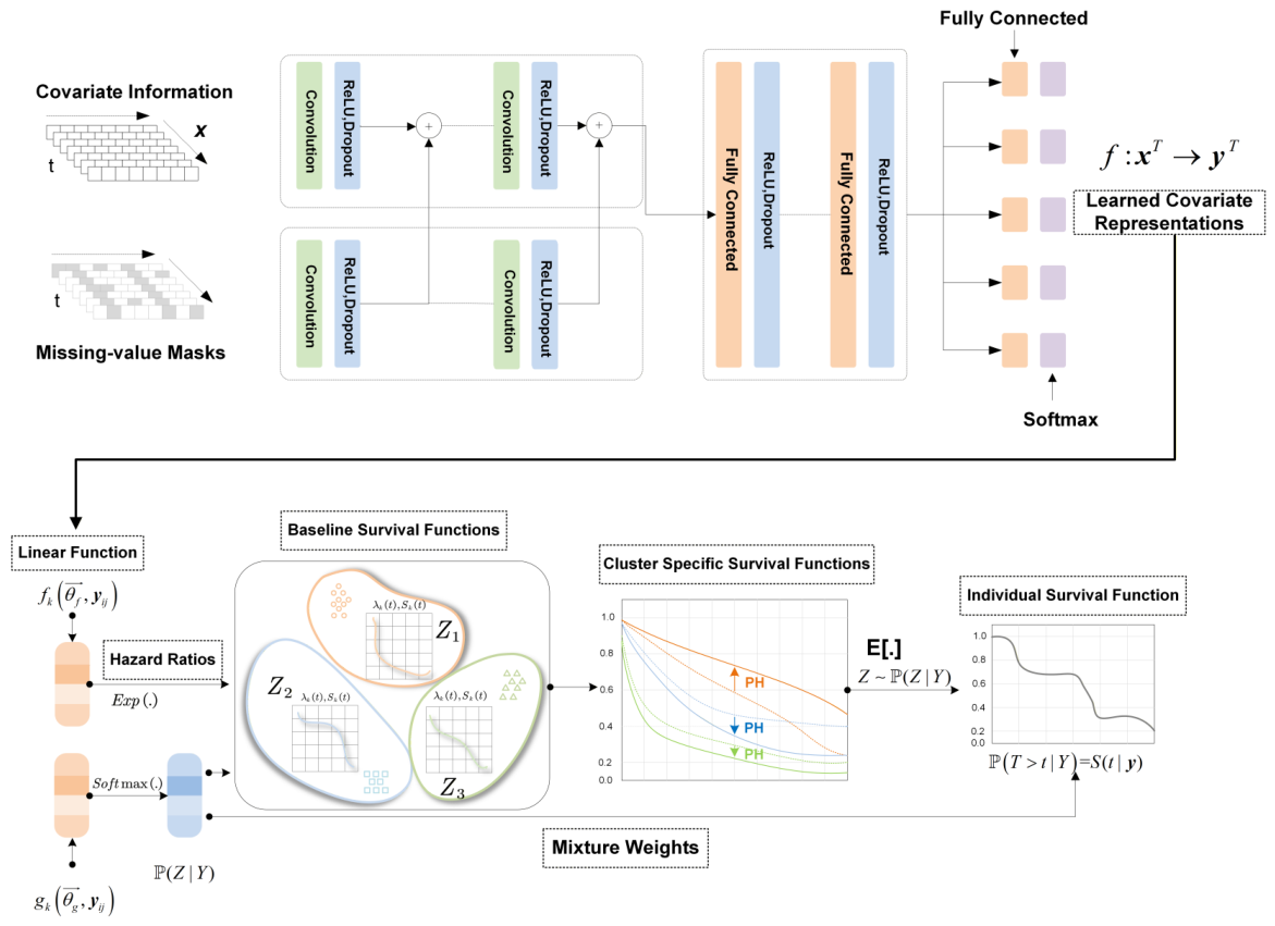
As illustrated in Figure 1, to handle partially missing values in longitudinal data, this study constructs a corresponding binary missing-value mask for each longitudinal covariate. For observed values, standardization is first performed using parameters estimated from the training fold. For missing values, their standardized numerical channels are set to 0, and the corresponding masks are set to 1. The inputs to the TCN consist of longitudinal features and the corresponding missing-value masks. The TCN first extracts local features from the temporal patterns of the data using dilated causal convolution blocks (labeled as “Convolution” blocks in Figure 1) to learn the underlying patterns of longitudinal covariates. Residual blocks are incorporated to refine the feature mapping, thereby mitigating the vanishing and exploding gradient problems in deep networks and improving computational efficiency, ultimately yielding learned covariate representations. Rectified linear unit (ReLU) functions are applied as nonlinear activation functions after each network layer to further alleviate the vanishing gradient issue. Dropout layers are adopted to randomly deactivate a proportion of neural units during training with a predefined probability, thereby reducing model overfitting. For individual i, the original covariate vector $x_{ij}$ observed at the j-th follow-up time point is transformed by the temporal convolutional network into the learned covariate representation $y_{ij}$. This representation encodes all longitudinal covariate information observed for individual i up to and including time $t_i$.

2.3. Deep Cox Mixtures Model

As shown in Figure 1, the Deep Cox Mixtures model assumes that each individual’s survival distribution can be represented as a finite mixture of K Cox models, where K is the number of latent Cox components. The mixture weight of the k-th latent component is determined from the individual’s covariates through the gating function $g(·)$. When $K=1$, the latent-component probability is identically one, the latent Cox mixture structure disappears, and the model reduces to a single TCN-Cox model. The procedure used to select the number of latent Cox components is described in Section 2.5.1.

The full likelihood function of the Deep Cox Mixtures model is formulated as follows:

$$\mathcal{L}\left(\mathit{\theta },{\left\{{\mathrm{\Lambda }}_k\right\}}_{k=1}^K\right)={\displaystyle \prod _{i=1}^{\left|\mathcal{D}\right|}}{\displaystyle \prod _{j=1}^{J_i}}{\displaystyle \sum _{k=1}^K}{\left[{\lambda }_k\left(t_i\mid {\mathbf{y}}_{ij}\right)\right]}^{{\delta }_i}{S}_k\left(t_i\mid {\mathbf{y}}_{ij}\right)\mathbb{P}\left(Z=k\mid {\mathbf{y}}_{ij}\right).$$

(2)

Here, $\overrightarrow{\theta }$ denotes the collection of neural network parameters, and ${\mathrm{\Lambda }}_k$ denotes the baseline cumulative hazard function for the k-th latent Cox cluster, which is estimated using the Breslow estimator as follows:

$${\widehat{\mathrm{\Lambda }}}_k\left(t\right)=\sum _{i:t_i<t}{\displaystyle \frac{1}{{\displaystyle \sum _{j\in {\mathcal{R}}_k\left(t_i\right)}}exp\left\{f_k({\widehat{\theta }}_f,y_j)\right\}}},$$

where the risk set ${\mathcal{R}}_k\left(t_i\right)$ is a set of individuals in the k-th latent cluster that survived beyond time $t_i$. For the k-th latent cluster, the hazard function is

$${\lambda }_k\left(t_i|y_{ij}\right)={\lambda }_k\left(t_i\right)exp\left(f_k\left(\overrightarrow{{\theta }_f},y_{ij}\right)\right),$$

where ${\lambda }_k\left(t_i\right)$ denotes the baseline hazard function of the k-th latent Cox cluster, and $f_k\left(\overrightarrow{{\theta }_f},y_{ij}\right)$ denotes the cluster-specific log-hazard function. The corresponding survival function is

$$S_k\left(t_i|y_{ij}\right)=exp\{-{\int }_0^{t_i}{\lambda }_k\left(s\right)exp(f_k({\overrightarrow{\theta }}_f,y_{ij}))ds\}=S_k{\left(t_i\right)}^{exp\left(f_k\left(\overrightarrow{{\theta }_f},y_{ij}\right)\right)},$$

where $S_k\left(t_i\right)$ denotes the baseline survival function of the k-th latent Cox cluster. The mixture weight is given by

$$\mathbb{P}\left(Z=k\mid y_{ij}\right)={softmax}_k\left(g\left(\overrightarrow{{\theta }_g},y_{ij}\right)\right).$$

Here, $g\left(\overrightarrow{{\theta }_g},y_{ij}\right)$ is the output of the gating function, and ${softmax}_k(·)$ denotes the k-th element of the softmax output. Specifically, let ${\mathbf{a}}_{ij}=g_{\theta }\left({\mathbf{h}}_{ij}\right)=\left(a_{ij1},\dots ,a_{ijK}\right)$ be the K-dimensional vector of gating logits computed from the TCN representation ${\mathbf{h}}_{ij}$. Through the softmax function, the mixture weight of the k-th latent Cox component is defined as

$${\pi }_{ijk}={softmax}_k\left({\mathbf{a}}_{ij}\right)={\displaystyle \frac{exp\left(a_{ijk}\right)}{{\sum }_{\mathit{\ell }=1}^{K}exp\left(a_{ij\mathit{\ell }}\right)}},k=1,\dots ,K.$$

(3)

Consequently, for every individual i and follow-up time $t_{ij}$, the mixture weights satisfy ${\pi }_{ijk}>0$ and ${\displaystyle \sum _{k=1}^K}{\pi }_{ijk}=1$. The quantity ${\pi }_{ijk}$ can therefore be interpreted as the model-estimated probability that the observation at $t_{ij}$ belongs to the k-th latent Cox component.

The gating function $g(·)$ and the linear function $f(·)$ are implemented using fully connected layers. They take the learned covariate representations to estimate the cluster-specific log-hazard function $f_k\left(\overrightarrow{{\theta }_f},y_{ij}\right)$ within each Cox model and the mixture weights $\mathbb{P}\left(Z=k|y_{ij}\right)$, respectively.

The identifiability of TCN-DCM is primarily affected by label switching in the mixture model and by non-unique neural-network parameterizations. Arbitrarily permuting the latent-component labels together with the corresponding gating probabilities, component-specific risk functions, and baseline survival functions leaves the overall mixture survival distribution unchanged; therefore, the numerical labels of the latent components have no fixed intrinsic meaning. In addition, different parameterizations of the TCN, gating network, and component-specific risk network may represent the same or approximately the same input-output function, so individual neural-network weights are not strictly uniquely identifiable. Practical weak identifiability may also arise when two latent components learn highly similar risk structures.

Accordingly, we do not claim strict global identifiability of every network parameter; instead, we focus on the stability of the overall survival distribution, individualized predictions, and latent risk structure.

2.4. Expectation–Maximization Algorithm

To solve the full likelihood function of the proposed model, two sets of covariate-dependent unknown parameters need to be estimated. The cluster-specific log-risk function $f_k\left(\overrightarrow{{\theta }_f},y_{ij}\right)$ and the gating function $g_k\left(\overrightarrow{{\theta }_g},y_{ij}\right)$ are expressed as

$$f_k\left(\overrightarrow{{\theta }_f},y_{ij}\right)={\theta }_{f1}{y}_{ij1}+{\theta }_{f2}{y}_{ij2}+\dots +{\theta }_{fm}{y}_{ijm},$$

$$g_k\left(\overrightarrow{{\theta }_g},y_{ij}\right)={\theta }_{g1}{y}_{ij1}+{\theta }_{g2}{y}_{ij2}+\dots +{\theta }_{gm}{y}_{ijm}.$$

Here, $y_{ijm}$ denotes the m-th element of the learned covariate representation $y_{ij}$.

Due to the large number of parameters to be estimated, it is intractable to obtain the optimal solution directly by maximizing the likelihood function. Therefore, this paper incorporates the initial values of $f_k\left(\overrightarrow{{\theta }_f},y_{ij}\right)$ and $g_k\left(\overrightarrow{{\theta }_g},y_{ij}\right)$ derived from the temporal convolutional network in Section 2.2 into the expectation–maximization (EM) algorithm for parameter estimation [16]. For notational simplicity, $y_i$ denotes the learned covariate representations used for individual i.

The approximate Monte Carlo expectation–maximization (MCEM) algorithm for the Deep Cox Mixtures model is described below [17].

2.4.1. E-Step

In this step, we calculate the posterior probability ${\gamma }_i$ of each individual belonging to the k-th latent cluster.

Since

$${\gamma }_i=\mathbb{P}\left(Z\right|T,Y)\propto \mathbb{P}\left(T\right|Z,Y)=\mathbb{P}{(T=t|Y,Z)}^{{\delta }_i}\mathbb{P}{(T>t|Y,Z)}^{1-{\delta }_i},$$

based on the expressions for the hazard function

$${\lambda }_k\left(t|y_i\right)={\lambda }_k\left(t\right)exp\left(f_k\left(\overrightarrow{{\theta }_f},y_i\right)\right),$$

and the survival probability function

$$S_k\left(t\right|y_i)=S_k{\left(t\right)}^{exp\left(f_k(\overrightarrow{{\theta }_f},y_i)\right)},$$

we derive the event probability estimates as follows:

$$\widehat{\mathbb{P}}\left(T>t\mid Y={\mathbf{y}}_i,Z=k\right)={\widehat{S}}_k{\left(t\right)}^{exp\left\{f_k({\widehat{\mathit{\theta }}}_f,{\mathbf{y}}_i)\right\}},$$

(4a)

$$\widehat{\mathbb{P}}\left(T=t\mid Y={\mathbf{y}}_i,Z=k\right)=-exp\left\{f_k({\widehat{\mathit{\theta }}}_f,{\mathbf{y}}_i)\right\}{\displaystyle \frac{{\widehat{S}}_k{\left(t\right)}^{exp\left\{f_k({\widehat{\mathit{\theta }}}_f,{\mathbf{y}}_i)\right\}}}{{\widehat{S}}_k\left(t\right)}}{\displaystyle \frac{\mathit{\partial }}{\mathit{\partial }t}}{\widehat{S}}_k\left(t\right).$$

(4b)

Here, the baseline survival function ${\widehat{S}}_k\left(t\right)$ is estimated using polynomial spline interpolation.

2.4.2. M-Step

The objective function is defined as

$$Q\left(\mathit{\theta }\right)={\displaystyle \sum _{i=1}^{\left|\mathcal{D}\right|}}{\displaystyle \sum _{k=1}^K}\left[{\gamma }_i^{k}log\mathbb{P}(Z=k\mid Y={\mathbf{y}}_i)+{\zeta }_i^{k}log\mathbb{P}(T=t_i\mid Z=k,Y={\mathbf{y}}_i)\right].$$

(5)

Here, ${\gamma }_i\in [0,1]$ is the posterior probability obtained from the E-step.

Since ${\gamma }_i\propto \mathbb{P}\left(T_i\right|Z_i=k,Y=y_i)$, we use ${\zeta }_i\sim \mathrm{Categorical}\left({\gamma }_i\right)$ as a substitute during parameter inference.

The estimator of $Q(\overrightarrow{\theta })$ is given by

$$\widehat{Q}\left(\mathit{\theta }\right)={\displaystyle \sum _{i=1}^{|{\mathcal{D}}_b|}}{\displaystyle \sum _{k=1}^K}{\gamma }_i^k\log {\mathrm{softmax}}_k\left(g({\mathit{\theta }}_g,{\mathbf{y}}_i)\right)+{\displaystyle \sum _{k=1}^K}log\mathcal{PL}\left({\mathcal{D}}_b^k,\mathit{\theta }\right).$$

(6)

Here, ${\mathcal{D}}_b$ denotes the b-th mini-batch of longitudinal data, and ${\mathcal{D}}_b^k$ represents the subset of longitudinal data belonging to the k-th latent cluster within the b-th mini-batch. $\mathcal{P}\mathcal{L}\left({\mathcal{D}}_b^k,\overrightarrow{\theta }\right)$ is the partial likelihood function based on the Cox model for the k-th latent cluster. The notation ${softmax}_k(·)$ denotes the k-th element of the softmax output, corresponding to the estimated mixture weight of the k-th latent cluster.

The MCEM algorithm does not directly estimate or impute missing longitudinal covariates. It is used only to handle the unobserved latent Cox components and, based on the longitudinal representation, to compute posterior responsibilities and update the model parameters. Specifically, let M denote the number of Monte Carlo latent-component allocations used in each parameter update. According to the posterior responsibilities obtained in the E-step, M sets of component labels are sampled independently, and the corresponding within-component Cox losses are averaged; the gating loss is calculated directly from the posterior responsibilities. When $M>1$, the Breslow baseline survival estimates obtained from the multiple allocations are averaged on a common time grid.

To assess whether generative representation regularization improves longitudinal survival prediction, we additionally considered an optional variational autoencoder (VAE) auxiliary branch during model development.

For individual i at observation time j, the TCN representation $h_{\mathrm{ij}}$ is processed by the VAE encoder to produce a mean vector ${\mu }_{\mathrm{ij}}$ and a log-variance vector $log{\sigma }_{\mathrm{ij}}^2$ for the latent-variable distribution. During training, the latent variable is obtained by the reparameterization trick as

$$z_{\mathrm{ij}}={\mu }_{\mathrm{ij}}+{\sigma }_{\mathrm{ij}}\odot {\epsilon }_{\mathrm{ij}},{\epsilon }_{\mathrm{ij}}\sim N(0,I),$$

$${\mathcal{L}}_{\mathrm{VAE}}={\mathcal{L}}_{\mathrm{rec}}+{\mathcal{L}}_{\mathrm{KL}},$$

$$\mathcal{L}(\mathrm{\Theta };\alpha )={\mathcal{L}}_{\mathrm{Cox}}+{\mathcal{L}}_{\mathrm{gate}}+\alpha {\mathcal{L}}_{\mathrm{VAE}}.$$

Meanwhile, considering both $\widehat{Q}\left(\overrightarrow{\theta },{\mathcal{D}}_b\right)$ and the information loss induced by variational autoencoder (VAE) encoding, the loss function is formulated as

$$Loss\left(\mathit{\theta },{\mathcal{D}}_b\right)=\widehat{Q}\left(\mathit{\theta },{\mathcal{D}}_b\right)+\alpha {Loss}_{\mathrm{VAE}}\left(\mathit{\theta },{\mathcal{D}}_b\right).$$

(7)

Here, ${\mathrm{Loss}}_{\mathrm{VAE}}={\mathcal{L}}_{\mathrm{VAE}}$, and the latent representation is sampled from a Gaussian prior with zero mean and identity covariance matrix [18].

After each epoch, the average negative approximate Q-function was evaluated on the validation set. Training was terminated when either the prespecified maximum number of epochs was reached or the validation loss increased relative to the preceding epoch for three consecutive epochs. The total training and validation losses, component-wise Cox and gating losses, and computation time were recorded at every epoch for numerical convergence diagnostics.

By minimizing the loss function, we update the parameter set $\overrightarrow{\theta }$ and the baseline survival function ${\widehat{S}}_k\left(t\right)$ for each latent cluster. The estimated survival probability of an individual at time t is calculated as

$$\begin{array}{cc}\hfill \widehat{\mathbb{P}}\left(T>t\mid Y={\mathbf{y}}_i\right)& ={\mathbb{E}}_{Z\sim \widehat{\mathbb{P}}(Z\mid Y)}\left[\widehat{\mathbb{P}}\left(T>t\mid Y={\mathbf{y}}_i,Z\right)\right]\hfill \\ \hfill & ={\displaystyle \sum _{k=1}^K}{\widehat{S}}_k{\left(t\right)}^{exp\left\{f_k({\widehat{\mathit{\theta }}}_f,{\mathbf{y}}_i)\right\}}{softmax}_k\left(g({\widehat{\mathit{\theta }}}_g,{\mathbf{y}}_i)\right).\hfill \end{array}$$

(8)

We did not calculate parameter-wise standard errors or an inverse Fisher information matrix for the high-dimensional parameters of the TCN, gating network, and component-specific risk networks. Because the objective is non-convex, the mixture components are subject to label switching, and the optimization involves stochastic Monte Carlo component allocations, uncertainty approximations based on a local Hessian or observed information matrix may be numerically unstable and difficult to interpret for individual neural-network weights.

2.5. Model Specification and Sensitivity Analyses

To ensure comparability across model configurations, all parameter-selection, internal-ablation, and sensitivity analyses used the same patient-level cross-validation folds, input variables, within-fold preprocessing, initialization rules, training procedure, stopping criteria, and evaluation horizons. In each comparison, only the model component or parameter under investigation was changed, while all remaining settings were held fixed.

Candidate configurations were evaluated using the time-dependent concordance index $C^{\mathrm{td}}$, dynamic AUC, and Brier score, together with the composite metric

$$Score={\displaystyle \frac{C^{\mathrm{td}}+AUC+(1-BS)}{3}}.$$

Definitions of $C^{\mathrm{td}}$, AUC, and BS are provided in Section 3.2.

Higher values of $C^{\mathrm{td}}$ and AUC and lower values of BS yield a higher Score. To avoid selecting an unnecessarily complex model because of a negligible numerical difference, we used a parsimony rule: if the Score of a structurally simpler candidate was within 0.005 of the highest Score, the simplest such candidate was selected; otherwise, the configuration with the highest Score was selected. Complete parameter-selection and ablation results are reported in Appendix A.

2.5.1. Selection of the Number of Latent Cox Components

The number of latent Cox components K determines the complexity with which the model represents individual-level risk heterogeneity. A smaller K gives a simpler structure but may not adequately characterize latent risk differences, whereas a larger K increases flexibility but may introduce redundant components and reduce the stability of estimation and component interpretation.

Accordingly, we systematically compared $K\in \{1,2,3,4,5,6\}$. During the comparison of K, the VAE weight, number of Monte Carlo draws, network architecture, number of training epochs, data-preprocessing procedure, random-initialization rule, and cross-validation folds were held fixed, so that differences across configurations primarily reflected the number of latent Cox components.

2.5.2. Selection of the VAE Weight and Number of Monte Carlo Draws

To evaluate the effect of VAE auxiliary regularization on dynamic survival prediction, we considered

$$\alpha \in \{0,0.01,0.1,1\},$$

where $\alpha =0$ denotes the absence of the VAE reconstruction-loss and KL-divergence constraints, whereas the remaining values represent different strengths of auxiliary regularization. For each fixed number of Monte Carlo draws, $\alpha =0$ was compared with the positive VAE weights to determine whether the auxiliary task produced a stable predictive benefit. Allowing $\alpha =0$ to be selected avoided assuming in advance that VAE regularization must improve predictive performance.

Let M denote the number of Monte Carlo latent-component allocations used in each MCEM parameter update. We compared

$$M\in \{1,5,10\}.$$

For a fixed VAE weight, models with different M values were trained using identical data partitions, network architecture, and stopping criteria. This comparison assessed whether additional Monte Carlo draws reduced variation induced by stochastic component allocation and whether any predictive benefit justified the additional computational cost.

After determining K, the candidate combinations of $\alpha$ and M were compared systematically, and the configuration for each data setting was selected according to the composite Score and parsimony rule.

2.5.3. Internal Ablation and Optimization-Stability Analyses

To quantify the contribution of each TCN-DCM component, we conducted the following internal ablation and sensitivity analyses using both the simulated and PBC data.

First, to evaluate the contribution of the masked causal dilated TCN temporal-representation module, the TCN encoder was replaced by landmark-safe cumulative mean pooling to construct a Mean-pooling DCM. This model summarized only longitudinal information available at or before the current landmark time while retaining the missingness indicators, latent Cox mixture structure, and all remaining training settings.

Second, to evaluate the contribution of the Deep Cox latent-mixture structure, the number of latent Cox components was fixed at $K=1$, yielding a TCN-Cox model. This model retained the TCN temporal encoder but removed the multi-component mixture structure and latent-component assignment mechanism. Because $K=1$ was also a candidate in the component-number sensitivity analysis, the same result was used to quantify the independent contribution of the mixture structure.

Third, at the same M, the contribution of the VAE component was evaluated by comparing $\alpha =0$ with the positive VAE weights. The MCEM estimation procedure cannot be removed while retaining the same latent-mixture likelihood; therefore, we compared different values of the number of Monte Carlo draws M and combined these comparisons with fold-level convergence diagnostics to evaluate the predictive and numerical stability of the MCEM implementation.

To evaluate the sensitivity of MCEM optimization to parameter initialization, four prespecified random seeds were examined. Because neural-network parameters admit hidden-unit permutations, rescaling, and other non-unique representations, individual network weights were not compared element by element across initializations. Instead, practical sensitivity was assessed using out-of-fold $C^{\mathrm{td}}$, AUC, BS, the composite Score, and the standard deviation of the Score. The model outputs did not exhibit strong practical sensitivity to the initialization schemes examined.

For each fold, we also recorded the best-validation epoch, stopping epoch, minimum validation loss, and validation loss at stopping, and calculated the proportion of valid training histories to assess the numerical convergence of MCEM optimization. Complete internal-ablation, parameter-sensitivity, random-initialization, and convergence-diagnostic results are provided in

Table A1. Ablation of the temporal-representation module.

Scenario	Temporal Representation	Mean Ctd	Mean AUC	Mean BS	Score
PH	Masked causal dilated TCN	0.7834	0.7878	0.0259	0.8484
PH	Mean-pooling DCM	0.7827	0.7879	0.0268	0.8480
non-PH	Masked causal dilated TCN	0.5946	0.6020	0.1013	0.6984
non-PH	Mean-pooling DCM	0.5921	0.6018	0.1021	0.6973
PBC	Masked causal dilated TCN	0.8133	0.8543	0.1550	0.8375
PBC	Mean-pooling DCM	0.7915	0.8365	0.1584	0.8232

Note: Bold type identifies the masked causal dilated TCN representation retained in the final model for each scenario.

,

Table A2. Sensitivity to the number of latent Cox components.

Scenario	K	Mean Ctd	Mean AUC	Mean BS	Score (SD)
PH	1	0.7147	0.7166	0.0237	0.8025 (0.0355)
PH	2	0.7957	0.7996	0.0262	0.8563 (0.0309)
PH	3	0.7835	0.7873	0.0262	0.8482 (0.0345)
PH	4	0.7810	0.7840	0.0261	0.8463 (0.0354)
PH	5	0.7932	0.7976	0.0258	0.8550 (0.0354)
PH	6	0.7975	0.8014	0.0251	0.8579 (0.0318)
non-PH	1	0.5737	0.5797	0.0977	0.6852 (0.0227)
non-PH	2	0.5827	0.5897	0.1011	0.6904 (0.0205)
non-PH	3	0.5906	0.5973	0.1026	0.6951 (0.0183)
non-PH	4	0.5939	0.6006	0.1013	0.6978 (0.0183)
non-PH	5	0.5976	0.6046	0.1023	0.7000 (0.0191)
non-PH	6	0.5998	0.6076	0.1022	0.7017 (0.0199)
PBC	1	0.7656	0.8038	0.1661	0.8011 (0.0324)
PBC	2	0.7897	0.8299	0.1587	0.8203 (0.0366)
PBC	3	0.8003	0.8387	0.1590	0.8267 (0.0328)
PBC	4	0.8038	0.8425	0.1514	0.8316 (0.0422)
PBC	5	0.8024	0.8427	0.1586	0.8288 (0.0343)
PBC	6	0.8127	0.8532	0.1536	0.8374 (0.0410)

Note: Bold type indicates the configuration selected according to the prespecified Score-based parsimony rule.

,

Table A3. Sensitivity to the VAE regularization weight.

Scenario	VAE Weight (α)	Fixed M	Mean Ctd	Mean AUC	Mean BS	Score
PH	0	1	0.7931	0.7964	0.0270	0.8542
PH	0.01	1	0.7960	0.7998	0.0260	0.8566
PH	0.1	1	0.7934	0.7972	0.0264	0.8547
PH	1	1	0.7969	0.8005	0.0263	0.8571
non-PH	0	1	0.5946	0.6020	0.1013	0.6984
non-PH	0.01	1	0.5939	0.6006	0.1013	0.6978
non-PH	0.1	1	0.5953	0.6021	0.1013	0.6987
non-PH	1	1	0.5962	0.6030	0.1014	0.6993
PBC	0	5	0.8133	0.8542	0.1550	0.8375
PBC	0.01	5	0.8078	0.8493	0.1565	0.8335
PBC	0.1	5	0.8040	0.8463	0.1574	0.8310
PBC	1	5	0.8088	0.8502	0.1559	0.8344

Note: Bold type indicates the configuration selected according to the prespecified Score-based parsimony rule.

,

Table A4. Sensitivity to the number of Monte Carlo draws.

Scenario	M	Fixed (α)	Mean Ctd	Mean AUC	Mean BS	Score
PH	1	0	0.7931	0.7964	0.0270	0.8542
PH	5	0	0.7955	0.7994	0.0270	0.8559
PH	10	0	0.7946	0.7988	0.0261	0.8558
non-PH	1	0	0.5946	0.6020	0.1013	0.6984
non-PH	5	0	0.5948	0.6018	0.1007	0.6987
non-PH	10	0	0.5918	0.5987	0.1026	0.6960
PBC	1	0	0.7949	0.8335	0.1577	0.8236
PBC	5	0	0.8133	0.8542	0.1550	0.8375
PBC	10	0	0.8081	0.8487	0.1505	0.8354

Note: Bold type indicates the configuration selected according to the prespecified Score-based parsimony rule.

,

Table A5. Sensitivity to random initialization in the PH scenario.

Random Seed	Ctd	AUC	BS	Score Mean (SD)
11	0.7237	0.7285	0.0161	0.8120 (0.1184)
111	0.7458	0.7548	0.0171	0.8278 (0.0893)
2026	0.7218	0.7264	0.0178	0.8101 (0.1180)
9999	0.7442	0.7497	0.0177	0.8254 (0.0986)
Median	0.7340	0.7391	0.0174	0.8187 (0.1083)

,

Table A6. Sensitivity to random initialization in the non-PH scenario.

Random Seed	Ctd	AUC	BS	Score Mean (SD)
11	0.5572	0.5682	0.0940	0.6771 (0.0310)
111	0.5664	0.5736	0.0963	0.6812 (0.0288)
2026	0.5633	0.5711	0.0942	0.6801 (0.0455)
9999	0.5723	0.5798	0.0931	0.6864 (0.0315)
Median	0.5649	0.5724	0.0941	0.6807 (0.0313)

,

Table A7. Sensitivity to random initialization in the PBC data.

Random Seed	Ctd	AUC	BS	Score Mean (SD)
11	0.7966	0.8314	0.1606	0.8225 (0.0498)
111	0.8109	0.8499	0.1537	0.8357 (0.0439)
2026	0.8009	0.8334	0.1618	0.8242 (0.0582)
9999	0.8072	0.8426	0.1547	0.8317 (0.0436)
Median	0.8041	0.8380	0.1577	0.8280 (0.0469)

,

Table A8. Fold-level numerical convergence diagnostics for TCN-DCM in the PH simulation.

Repeat	Fold	Best-Validation Epoch	Stopping Epoch	Minimum Validation Loss	Validation Loss at Stopping
1	1	43.0	48.5	4.9563	6.0216
1	2	54.0	60.5	6.1733	7.2137
1	3	45.5	50.5	4.5756	5.2237
1	4	61.0	69.0	4.4188	4.8979
1	5	63.5	67.0	5.8520	6.2788
2	1	1.0	4.0	10.5649	10.7012
2	2	55.5	67.0	5.8193	6.7646
2	3	49.0	57.5	4.7020	5.2775
2	4	68.0	82.0	6.2841	6.9319
2	5	50.0	55.0	5.1367	5.6402
Summary		52.0(46.4–59.6)	59.0(51.6–67.0)	5.4780(4.7656–6.0930)	6.1502(5.3682–6.8900)

Note: Bold type identifies the summary row. Summary values are presented as median (IQR).

,

Table A9. Fold-level numerical convergence diagnostics for TCN-DCM in the non-PH simulation.

Repeat	Fold	Best-Validation Epoch	Stopping Epoch	Minimum Validation Loss	Validation Loss at Stopping
1	1	19.5	24.5	55.8545	56.4814
1	2	18.0	22.5	55.7115	56.1261
1	3	12.5	22.5	53.8232	54.4259
1	4	12.0	23.5	59.6074	60.2503
1	5	23.0	34.0	52.5281	52.9084
2	1	11.5	18.0	58.8098	59.3674
2	2	21.5	27.5	55.3737	55.5861
2	3	30.5	33.5	55.9574	56.7735
2	4	20.5	30.5	53.2925	54.9849
2	5	7.5	14.0	57.0773	57.3991
Summary	—	18.8(12.1–21.3)	24.0(22.5–29.8)	55.7830(54.2108–56.7973)	56.3037(55.1352–57.2427)

Note: Bold type identifies the summary row. Summary values are presented as median (IQR).

and

Table A10. Fold-level numerical convergence diagnostics for TCN-DCM on the PBC data.

Repeat	Fold	Best-Validation Epoch	Stopping Epoch	Minimum Validation Loss	Validation Loss at Stopping
1	1	41	44	13.3173	13.8697
1	2	42	45	15.6902	16.2296
1	3	36	39	18.5957	18.7610
1	4	43	46	17.4578	17.7784
1	5	53	76	14.9128	15.3553
2	1	27	41	18.2836	19.1564
2	2	37	40	12.7060	13.0404
2	3	54	57	12.6083	12.9675
2	4	82	85	15.5493	17.1518
2	5	40	41	12.5163	12.8199
Summary	—	41.5 (37.8–50.5)	44.5 (41.0–54.3)	15.2311 (12.8588–17.0159)	15.7925 (13.2477–17.6218)

Note: Bold type identifies the summary row. Summary values are presented as median (IQR).

.

Code for simulation-data generation and the TCN-DCM model is provided in the Supplementary Materials.

3. Simulation Study

3.1. Simulation Scenarios

Data were generated using a JM. The longitudinal process with j time points was modeled using a linear mixed-effects model, which incorporates the main effects of 10 binary baseline covariates, as well as a random intercept and a random slope [19].

$$y_{ij}\left(t\right)=m_{ij}\left(t\right)+{\epsilon }_{ij}\left(t\right)={\mathbf{x}}_{ij}^{\prime }{\mathit{\beta }}_j+{\mathbf{z}}_{ij}^{\prime }{\mathbf{b}}_{ij}+{\epsilon }_{ij}\left(t\right),$$

(9)

where $y_{ij}\left(t\right)$ denotes one longitudinal measurement of individual i at time point t; $x_{ij}$ and $z_{ij}$ are covariate vectors associated with the fixed-effect vector ${\beta }_j$ and the random-effect vector $b_{ij}$, respectively. The random-effect vector follows a zero-mean normal distribution $b_{ij}\sim N\left(0,G_j\right)$, where $G_j$ is the variance-covariance matrix. The covariate vectors are independent of the random error ${\epsilon }_{ij}\left(t\right)\sim N\left(0,{{\sigma }_j}^2\right)$. The observed estimate of each latent longitudinal covariate is $m_{ij}\left(t\right)$, which includes

$$x_{ij}={\left(1,t,X_{i1},X_{i2},X_{i3}\right)}^{\prime },$$

$$X_{i1},X_{i2},X_{i3}\sim Bernoulli\left(p\right),$$

$$z_{ij}={\left(1,t\right)}^{\prime }.$$

In Scenario (1), the simulated data followed a standard joint-model specification in which the event hazard depended on the current longitudinal value. Scenario (2) incorporated both a time-varying effect of the current longitudinal marker and a cumulative historical-average effect, causing the association between the longitudinal marker and event risk to change over time and thereby strengthening the violation of the global PH assumption.

Scenario (1):

$$h_i\left(t\right)=h_0\left(t\right)exp\left\{{\gamma }^{\prime }{\mathbf{w}}_i+{\alpha }_1{m}_{ij}\left(t\right)\right\}.$$

(10a)

Scenario (2):

$$h_i\left(t\right)=h_0\left(t\right)exp\left\{{\gamma }^{\prime }{\mathbf{w}}_i+\alpha \left(t\right){\tilde{m}}_i\left(t\right)+\eta {\overline{m}}_i\left(t\right)\right\},$$

(10b)

where

$$w_i={\left(X_{i1},X_{i2},X_{i3}\right)}^{\prime },$$

$w_i$ is the vector of baseline covariates. $\alpha \left(t\right)=0.50-{\displaystyle \frac{t}{15}},\eta =0.40;{\tilde{m}}_i\left(t\right)$ denotes the standardized current longitudinal marker, and ${\overline{m}}_i\left(t\right)$ denotes its historical mean up to t. Let ${\mu }_m$ and ${\sigma }_m$ be the mean and sample standard deviation, respectively, of all $m_i\left(t_g\right)$ values. Then ${\tilde{m}}_i\left(t_g\right)={\displaystyle \frac{m_i\left(t_g\right)-{\mu }_m}{{\sigma }_m}}$. In addition, the standardized historical mean of the longitudinal marker up to time t is defined as ${\overline{m}}_i\left(t\right)={\displaystyle \frac{1}{t}}{\int }_0^t{\tilde{m}}_i\left(s\right)ds,t>0$.

The baseline hazard followed a Weibull distribution, specified as

$$h_0\left(t\right)=exp\left({\sigma }_1\right){\sigma }_2{t}^{{\sigma }_2-1}.$$

In addition, seven binary noise variables, $X_{i4},X_{i5},\dots ,X_{i10}$, were simulated as irrelevant covariates in the longitudinal data.

3.2. Performance Evaluation Metrics

We used twice-repeated patient-level five-fold cross-validation. In each repetition, approximately 80% of patients were used for model training and the remaining 20% for out-of-fold evaluation; the two partitions were generated using different prespecified random seeds, and all competing models used the same patient-level fold assignments.

The prediction windows t were set to $[2,3,4,5]$, and the predictive performance of the model was evaluated using the time-dependent concordance index $C^{\mathrm{td}}$, area under the ROC curve (AUC), and Brier score (BS).

For $C^{\mathrm{td}}$, we used the censoring-adjusted estimator proposed by Gerds [20], which is constructed based on the Kaplan–Meier estimator of the inverse probability of censoring weights (IPCW):

$$C^{\mathrm{td}}\left(t\right)=\mathbb{P}\left(\widehat{F}(t\mid {\mathbf{x}}_i)>\widehat{F}(t\mid {\mathbf{x}}_j)\mid {\delta }_i=1,T_i<T_j,T_i\le t\right).$$

(11)

The AUC adjusts sensitivity using the IPCW-based estimate of the censoring distribution [21]:

$$\widehat{Se}(c,t)={\displaystyle \frac{{\sum }_{i=1}^n{\omega }_{i}I\{{\pi }_i\left(t\right)>c,T_i\le t\}}{{\sum }_{i=1}^n{\omega }_{i}I\{T_i<t\}}},$$

(12a)

$$\begin{array}{cc}\hfill {\omega }_i& ={\displaystyle \frac{{\delta }_i}{n\widehat{G}\left(T_i\right)}},\hfill \end{array}$$

(12b)

$$\begin{array}{cc}\hfill \widehat{Sp}(c,t)& ={\displaystyle \frac{{\sum }_{i=1}^{n}I\{{\pi }_i\left(t\right)\le c,T_i>t\}}{{\sum }_{i=1}^{n}I\{T_i>t\}}},\hfill \end{array}$$

(12c)

where $\widehat{Se}(c,t)$ and $\widehat{Sp}(c,t)$ denote the estimated sensitivity and specificity at the classification threshold c and time point t, respectively. $\widehat{G}\left(t\right)$ is the Kaplan–Meier estimator of the censoring distribution, $I\left(·\right)$ is the indicator function, and ${\pi }_i\left(t\right)$ represents the survival probability $\mathbb{P}\left(T>t|X=x_i\right)$ estimated by the classifier.

The BS measures the mean squared error of binary predictions for event occurrence probabilities at the quantiles of event time. In general, a BS value of 0 indicates perfect prediction, while a BS value of 0.25 indicates performance no better than random guessing. A smaller BS value corresponds to more accurate prediction performance.

$${\widehat{BS}}_{\mathrm{IPCW}}\left(t\right)={\displaystyle \frac{1}{n}}{\displaystyle \sum _{i=1}^n}\left[{\displaystyle \frac{{\pi }_i{\left(t\right)}^{2}I\{T_i\le t,{\delta }_i=1\}}{\widehat{G}\left(T_i\right)}}+{\displaystyle \frac{{\{1-{\pi }_i\left(t\right)\}}^{2}I\{T_i>t\}}{\widehat{G}\left(t\right)}}\right].$$

(13)

3.3. Analysis of Simulation Results

According to the selection rules specified in Section 2.5.1 and Section 2.5.2, the final simulation analyses used $(K,\alpha ,M)=(2,0,1)$ under the PH scenario and $(K,\alpha ,M)=(4,0,1)$ under the non-PH scenario. Complete sensitivity results for K, $\alpha$, and M are provided in Table A2, Table A3 and Table A4.

In Scenario (1), where the PH assumption held (

Table 1. Simulation performance of survival data under the PH assumption.

		TCN-DCM		RDSM		DDH		JM
Metric	Horizon	Mean	SD	Mean	SD	Mean	SD	Mean	SD
$C^{\mathrm{td}}$	$t=2$	0.7789	0.0538	0.7285	0.0729	0.5509	0.0788	0.8307	0.0606
	$t=3$	0.7875	0.0438	0.7318	0.0731	0.5539	0.0762	0.8282	0.0616
	$t=4$	0.7851	0.0479	0.7300	0.0750	0.5478	0.0829	0.8244	0.0627
	$t=5$	0.7852	0.0493	0.7280	0.0755	0.5517	0.0838	0.8192	0.0644
AUC	$t=2$	0.7817	0.0535	0.7293	0.0740	0.5451	0.0784	0.8365	0.0616
	$t=3$	0.7915	0.0434	0.7333	0.0750	0.5460	0.0754	0.8362	0.0628
	$t=4$	0.7898	0.0488	0.7325	0.0777	0.5353	0.0826	0.8347	0.0641
	$t=5$	0.7908	0.0506	0.7300	0.0788	0.5344	0.0847	0.8321	0.0665
BS	$t=2$	0.0140	0.0036	0.0126	0.0029	0.0124	0.0027	0.0131	0.0025
	$t=3$	0.0228	0.0054	0.0197	0.0041	0.0197	0.0041	0.0202	0.0036
	$t=4$	0.0315	0.0068	0.0268	0.0051	0.0272	0.0053	0.0269	0.0046
	$t=5$	0.0404	0.0085	0.0344	0.0063	0.0354	0.0070	0.0339	0.0058

Note: Bold type indicates the best mean performance at each prediction horizon; tied best means are all shown in bold. Higher $C^{\mathrm{td}}$ and AUC values and lower BS values indicate better predictive performance.

), the simulated data were generated fully in accordance with the modeling assumptions of the joint model. The joint model was therefore expected to achieve the best predictive performance. Empirically, the joint model outperformed the other benchmark models in both $C^{\mathrm{td}}$ and AUC. TCN-DCM yielded $C^{\mathrm{td}}$ values of approximately 0.77–0.79, all AUC values exceeded 0.75, and all BS values were below 0.05, indicating favorable predictive performance on longitudinal data satisfying the PH assumption. TCN-DCM also generally outperformed RDSM and DDH, and its advantage did not diminish as the prediction horizon increased.

In Scenario (2), where the PH assumption was violated (

Table 2. Simulation performance of survival data under violation of the PH assumption.

		TCN-DCM		RDSM		DDH		JM
Metric	Horizon	Mean	SD	Mean	SD	Mean	SD	Mean	SD
$C^{\mathrm{td}}$	$t=2$	0.5977	0.0326	0.5777	0.0198	0.5351	0.0337	0.5264	0.0262
	$t=3$	0.5975	0.0330	0.5796	0.0207	0.5346	0.0340	0.5285	0.0282
	$t=4$	0.5968	0.0333	0.5801	0.0219	0.5339	0.0323	0.5297	0.0301
	$t=5$	0.5962	0.0340	0.5796	0.0226	0.5343	0.0308	0.5301	0.0311
AUC	$t=2$	0.6036	0.0332	0.5849	0.0213	0.5140	0.0350	0.5302	0.0259
	$t=3$	0.6061	0.0340	0.5903	0.0229	0.5043	0.0358	0.5341	0.0279
	$t=4$	0.6081	0.0347	0.5941	0.0250	0.4945	0.0344	0.5370	0.0300
	$t=5$	0.6102	0.0358	0.5967	0.0264	0.4871	0.0331	0.5391	0.0312
BS	$t=2$	0.0629	0.0050	0.0617	0.0047	0.1246	0.0211	0.0617	0.0048
	$t=3$	0.0896	0.0071	0.0870	0.0065	0.2806	0.0571	0.0873	0.0066
	$t=4$	0.1137	0.0093	0.1095	0.0079	0.2935	0.0554	0.1103	0.0081
	$t=5$	0.1350	0.0115	0.1294	0.0092	0.3053	0.0541	0.1307	0.0093

Note: Bold type indicates the best mean performance at each prediction horizon; tied best means are all shown in bold. Higher $C^{\mathrm{td}}$ and AUC values and lower BS values indicate better predictive performance.

), RDSM and TCN-DCM showed clearly superior predictive performance in different respects. The $C^{\mathrm{td}}$ of TCN-DCM remained close to 0.6, and all AUC values exceeded 0.6, whereas RDSM achieved lower BS values. Thus, TCN-DCM and RDSM showed comparable overall performance for longitudinal data violating the PH assumption. DDH was markedly weaker in both discrimination and prediction error, indicating limited suitability for this simulated non-PH setting. The $C^{\mathrm{td}}$ and AUC of the joint model were lower than those of TCN-DCM and RDSM, while its BS was close to that of RDSM and slightly better than that of TCN-DCM.

To compare the overall performance of TCN-DCM and RDSM under the non-PH scenario more formally, we conducted dataset-level paired analyses. After Holm correction, TCN-DCM achieved significantly higher $C^{\mathrm{td}}$ at all four evaluation horizons and significantly higher AUC at years 2 and 3, whereas RDSM achieved significantly lower BS at all four horizons. Thus, neither model dominated consistently across all metrics: TCN-DCM provided stronger discrimination, while RDSM had a modest advantage in prediction error. Complete paired differences, bootstrap 95% confidence intervals, and Holm-adjusted p-values are provided in

Table A11. Dataset-level paired comparison of TCN-DCM and RDSM in the non-PH simulation.

Metric	Prediction Horizon, Years	Paired Difference Δ	Bootstrap 95% CI	Holm-Adjusted p-Value
$C^{\mathrm{td}}$	2	0.0200	0.0086–0.0331	0.0092
$C^{\mathrm{td}}$	3	0.0179	0.0054–0.0305	0.0110
$C^{\mathrm{td}}$	4	0.0167	0.0040–0.0292	0.0076
$C^{\mathrm{td}}$	5	0.0167	0.0047–0.0290	0.0092
AUC	2	0.0187	0.0059–0.0327	0.0155
AUC	3	0.0158	0.0035–0.0283	0.0335
AUC	4	0.0141	0.0036–0.0252	0.0739
AUC	5	0.0135	0.0015–0.0257	0.0577
BS	2	−0.0012	−0.0018–0.0006	0.0043
BS	3	−0.0026	−0.0038–0.0014	0.0020
BS	4	−0.0042	−0.0059–0.0024	0.0015
BS	5	−0.0057	−0.0081–0.0032	0.0020

Note: Within each dataset and prediction horizon, results from the twice-repeated five-fold cross-validation were averaged before the paired analysis. For $C^{\mathrm{td}}$ and AUC, the paired difference was defined as $\Delta =\mathrm{TCN}-\mathrm{DCM}-\mathrm{RDSM}$. For BS, the paired difference was defined as $\Delta ={\mathrm{BS}}_{\mathrm{RDSM}}-{\mathrm{BS}}_{\mathrm{TCN}-\mathrm{DCM}}$. Positive values therefore favor TCN-DCM, whereas negative values favor RDSM. The 95% confidence intervals were obtained from 1000 dataset-level bootstrap resamples. The p-values were obtained from two-sided Wilcoxon signed-rank tests and adjusted using the Holm procedure across the comparisons of TCN-DCM with RDSM, DDH, and JM within each metric and prediction horizon.

.

To assess robustness across different data conditions, we additionally examined sample sizes $N=300,500,1000$, target censoring rates of 20%, 40%, and 60%, and missing rates of 0%, 10%, and 30%, while holding the remaining data-generating mechanisms and model-training settings fixed. Twenty independent simulated datasets were generated for each setting, and the same twice-repeated five-fold cross-validation procedure as in the primary analysis was used. In both the PH and non-PH scenarios, increasing sample size generally improved $C^{\mathrm{td}}$ and AUC and reduced the standard deviations of the metrics. Increasing missingness mainly reduced discrimination, with a more pronounced effect in the non-PH scenario. Across censoring rates of 20–60%, performance was generally stable, although some deterioration and greater variability appeared at higher censoring rates. Complete results are provided in

Table A12. Sensitivity to sample size.

Scenario	Sample Size	Horizon (Years)	Ctd Mean (SD)	AUC Mean (SD)	BS Mean (SD)
PH	300	2	0.7901 (0.0227)	0.8178 (0.0231)	0.1296 (0.0122)
PH	300	3	0.7878 (0.0221)	0.8275 (0.0223)	0.1526 (0.0143)
PH	300	4	0.7851 (0.0217)	0.8352 (0.0227)	0.1628 (0.0152)
PH	300	5	0.7821 (0.0216)	0.8404 (0.0234)	0.1674 (0.0158)
PH	500	2	0.7974 (0.0178)	0.8266 (0.0190)	0.1249 (0.0077)
PH	500	3	0.7932 (0.0188)	0.8335 (0.0208)	0.1468 (0.0106)
PH	500	4	0.7895 (0.0179)	0.8392 (0.0199)	0.1579 (0.0119)
PH	500	5	0.7865 (0.0177)	0.8449 (0.0199)	0.1622 (0.0127)
PH	1000	2	0.8089 (0.0090)	0.8395 (0.0093)	0.1170 (0.0048)
PH	1000	3	0.8048 (0.0090)	0.8469 (0.0095)	0.1373 (0.0059)
PH	1000	4	0.8017 (0.0092)	0.8538 (0.0103)	0.1464 (0.0069)
PH	1000	5	0.7994 (0.0096)	0.8605 (0.0108)	0.1489 (0.0068)
non-PH	300	2	0.5677 (0.0453)	0.5711 (0.0464)	0.0648 (0.0061)
non-PH	300	3	0.5681 (0.0453)	0.5732 (0.0471)	0.0934 (0.0088)
non-PH	300	4	0.5685 (0.0459)	0.5753 (0.0487)	0.1197 (0.0112)
non-PH	300	5	0.5684 (0.0472)	0.5769 (0.0513)	0.1436 (0.0133)
non-PH	500	2	0.5909 (0.0292)	0.5943 (0.0304)	0.0653 (0.0039)
non-PH	500	3	0.5913 (0.0292)	0.5964 (0.0311)	0.0932 (0.0054)
non-PH	500	4	0.5921 (0.0291)	0.5988 (0.0318)	0.1182 (0.0066)
non-PH	500	5	0.5926 (0.0286)	0.6010 (0.0320)	0.1406 (0.0075)
non-PH	1000	2	0.6121 (0.0238)	0.6172 (0.0243)	0.0624 (0.0020)
non-PH	1000	3	0.6115 (0.0239)	0.6191 (0.0248)	0.0891 (0.0029)
non-PH	1000	4	0.6111 (0.0241)	0.6211 (0.0254)	0.1129 (0.0037)
non-PH	1000	5	0.6109 (0.0242)	0.6235 (0.0259)	0.1341 (0.0044)

,

Table A13. Sensitivity to the target censoring rate.

Scenario	Target Censoring Rate	Horizon (Years)	Ctd Mean (SD)	AUC Mean (SD)	BS Mean (SD)
PH	20%	2	0.8023 (0.0150)	0.8308 (0.0155)	0.1193 (0.0071)
PH	20%	3	0.7983 (0.0155)	0.8378 (0.0164)	0.1411 (0.0090)
PH	20%	4	0.7952 (0.0153)	0.8448 (0.0164)	0.1515 (0.0102)
PH	20%	5	0.7933 (0.0158)	0.8520 (0.0176)	0.1552 (0.0115)
PH	40%	2	0.8002 (0.0164)	0.8301 (0.0171)	0.1239 (0.0085)
PH	40%	3	0.7953 (0.0172)	0.8363 (0.0180)	0.1449 (0.0100)
PH	40%	4	0.7918 (0.0171)	0.8423 (0.0185)	0.1553 (0.0116)
PH	40%	5	0.7889 (0.0169)	0.8477 (0.0181)	0.1591 (0.0121)
PH	60%	2	0.8001 (0.0221)	0.8322 (0.0249)	0.1277 (0.0137)
PH	60%	3	0.7938 (0.0231)	0.8376 (0.0270)	0.1492 (0.0179)
PH	60%	4	0.7887 (0.0243)	0.8425 (0.0275)	0.1568 (0.0209)
PH	60%	5	0.7850 (0.0237)	0.8490 (0.0254)	0.1563 (0.0219)
non-PH	20%	2	0.5907 (0.0237)	0.5953 (0.0249)	0.0648 (0.0046)
non-PH	20%	3	0.5912 (0.0238)	0.5981 (0.0258)	0.0929 (0.0064)
non-PH	20%	4	0.5915 (0.0236)	0.6008 (0.0264)	0.1179 (0.0080)
non-PH	20%	5	0.5915 (0.0233)	0.6030 (0.0269)	0.1404 (0.0092)
non-PH	40%	2	0.5958 (0.0247)	0.5996 (0.0258)	0.0636 (0.0043)
non-PH	40%	3	0.5955 (0.0245)	0.6011 (0.0260)	0.0914 (0.0064)
non-PH	40%	4	0.5953 (0.0245)	0.6028 (0.0265)	0.1166 (0.0082)
non-PH	40%	5	0.5950 (0.0246)	0.6044 (0.0272)	0.1390 (0.0097)
non-PH	60%	2	0.5830 (0.0257)	0.5878 (0.0264)	0.0662 (0.0036)
non-PH	60%	3	0.5826 (0.0260)	0.5897 (0.0272)	0.0948 (0.0052)
non-PH	60%	4	0.5825 (0.0264)	0.5919 (0.0280)	0.1204 (0.0065)
non-PH	60%	5	0.5822 (0.0270)	0.5938 (0.0290)	0.1434 (0.0075)

and

Table A14. Sensitivity to the missing rate.

Scenario	Missing Rate	Horizon (Years)	${\mathit{C}}^{\mathbf{td}}$ Mean (SD)	AUC Mean (SD)	BS Mean (SD)
PH	0%	2	0.8002 (0.0155)	0.8288 (0.0159)	0.1226 (0.0067)
PH	0%	3	0.7970 (0.0161)	0.8372 (0.0170)	0.1443 (0.0092)
PH	0%	4	0.7939 (0.0164)	0.8441 (0.0174)	0.1546 (0.0106)
PH	0%	5	0.7909 (0.0162)	0.8498 (0.0177)	0.1590 (0.0114)
PH	10%	2	0.7972 (0.0161)	0.8261 (0.0164)	0.1229 (0.0087)
PH	10%	3	0.7916 (0.0160)	0.8314 (0.0160)	0.1451 (0.0102)
PH	10%	4	0.7885 (0.0169)	0.8381 (0.0180)	0.1554 (0.0119)
PH	10%	5	0.7869 (0.0173)	0.8457 (0.0195)	0.1588 (0.0130)
PH	30%	2	0.7810 (0.0129)	0.8093 (0.0132)	0.1257 (0.0060)
PH	30%	3	0.7762 (0.0118)	0.8151 (0.0119)	0.1502 (0.0065)
PH	30%	4	0.7730 (0.0114)	0.8216 (0.0114)	0.1628 (0.0070)
PH	30%	5	0.7705 (0.0115)	0.8273 (0.0126)	0.1686 (0.0075)
non-PH	0%	2	0.5954 (0.0313)	0.6001 (0.0315)	0.0652 (0.0041)
non-PH	0%	3	0.5956 (0.0316)	0.6026 (0.0321)	0.0931 (0.0053)
non-PH	0%	4	0.5953 (0.0324)	0.6046 (0.0335)	0.1183 (0.0063)
non-PH	0%	5	0.5948 (0.0334)	0.6063 (0.0350)	0.1409 (0.0070)
non-PH	10%	2	0.5817 (0.0278)	0.5855 (0.0287)	0.0639 (0.0053)
non-PH	10%	3	0.5817 (0.0289)	0.5875 (0.0305)	0.0916 (0.0076)
non-PH	10%	4	0.5812 (0.0301)	0.5889 (0.0324)	0.1164 (0.0093)
non-PH	10%	5	0.5801 (0.0314)	0.5895 (0.0347)	0.1387 (0.0103)
non-PH	30%	2	0.5586 (0.0313)	0.5628 (0.0337)	0.0651 (0.0043)
non-PH	30%	3	0.5581 (0.0318)	0.5643 (0.0356)	0.0923 (0.0064)
non-PH	30%	4	0.5574 (0.0322)	0.5655 (0.0375)	0.1168 (0.0078)
non-PH	30%	5	0.5568 (0.0332)	0.5667 (0.0401)	0.1388 (0.0091)

Note: Each condition included 20 independently simulated datasets. Within each dataset, results from the twice-repeated five-fold cross-validation were first aggregated, after which the independent dataset was treated as the statistical unit. Values are reported as mean (SD) across the independent datasets. Only one design factor was varied at a time, while all remaining data-generating and training settings were held fixed.

.

4. Real-World Case Analysis for Dynamic Risk Prediction

The dataset originates from a clinical trial for primary biliary cholangitis (PBC) conducted at the Mayo Clinic and is a well-known longitudinal survival dataset widely used for evaluating survival and dynamic prediction models [22,23]. Over the 10-year enrollment period of the PBC trial, a total of 424 patients diagnosed with PBC were referred to the Mayo Clinic and met the eligibility criteria for a randomized controlled trial comparing D-penicillamine with placebo. The first 312 enrolled patients participated in the randomized trial: 158 patients received D-penicillamine treatment, while the remaining 154 patients were assigned to the placebo group. An additional 112 patients declined participation in the randomized trial but consented to routine laboratory measurements and long-term survival follow-up.

Each patient in the cohort has longitudinal covariates collected at multiple follow-up time points, yielding a total of 1945 observational records. The dataset includes 20 variables: time to death or censoring, event indicator, treatment assignment, age, sex, serum bilirubin, albumin, diuretic use, prothrombin time, hepatomegaly, ascites, serum aspartate aminotransferase (AST) reflecting liver function, histological disease stage, and other clinical indicators.

4.1. Evaluation Results of Dynamic Prediction Models

According to the selection rules specified in Section 2.5.1 and Section 2.5.2, the final PBC analysis used $(K,\alpha ,M)=(6,0,5)$. Complete sensitivity results are provided in Table A1, Table A2, Table A3 and Table A4.

To evaluate the fit and generalizability of TCN-DCM on real-world data independently, we applied twice-repeated patient-level five-fold cross-validation to the PBC data. TCN-DCM maintained stable out-of-fold discrimination at all three evaluation horizons. Complete out-of-fold evaluation results and 95% confidence intervals are provided in

Table A15. Repeated-cross-validation out-of-fold evaluation of TCN-DCM on the PBC data.

Evaluation Metric	Evaluation Horizon (Years)	Mean	SD	95% CI
$C^{\mathrm{td}}$	4	0.8339	0.0308	0.8146–0.8523
$C^{\mathrm{td}}$	6	0.7990	0.0295	0.7800–0.8154
$C^{\mathrm{td}}$	8	0.7680	0.0303	0.7490–0.7846
AUC	4	0.8734	0.0327	0.8541–0.8911
AUC	6	0.8373	0.0396	0.8142–0.8609
AUC	8	0.8054	0.0414	0.7804–0.8285
BS	4	0.1266	0.0375	0.1063–0.1495
BS	6	0.1626	0.0489	0.1364–0.1942
BS	8	0.1878	0.0448	0.1627–0.2144

Note: The 95% confidence intervals were obtained from 1000 bootstrap resamples.

.

Years 4, 6, and 8 were selected as prediction horizons. TCN-DCM and three competing models were used to predict individual survival probabilities up to these prespecified horizons. The $C^{\mathrm{td}}$, AUC, and BS results indicated strong overall performance of TCN-DCM (

Table 3. Prediction performance of different models on the PBC dataset.

		TCN-DCM		RDSM		DDH		JM
Metric	Horizon	Mean	SD	Mean	SD	Mean	SD	Mean	SD
$C^{\mathrm{td}}$	$t=4$	0.8339	0.0308	0.8143	0.0461	0.6800	0.1321	0.7994	0.0390
	$t=6$	0.7990	0.0295	0.7846	0.0453	0.6721	0.1071	0.7766	0.0428
	$t=8$	0.7680	0.0303	0.7530	0.0423	0.6224	0.1422	0.7495	0.0463
AUC	$t=4$	0.8734	0.0327	0.8536	0.0543	0.6997	0.1529	0.8413	0.0395
	$t=6$	0.8373	0.0396	0.8254	0.0659	0.6959	0.1220	0.8246	0.0554
	$t=8$	0.8054	0.0414	0.7897	0.0696	0.6318	0.1711	0.8061	0.0606
BS	$t=4$	0.1266	0.0375	0.1329	0.0401	0.2046	0.0720	0.1395	0.0306
	$t=6$	0.1626	0.0489	0.1602	0.0438	0.2519	0.0930	0.1652	0.0384
	$t=8$	0.1878	0.0448	0.1891	0.0415	0.3055	0.1220	0.1822	0.0405

Note: Bold type indicates the best mean performance at each prediction horizon. Higher $C^{\mathrm{td}}$ and AUC values and lower BS values indicate better predictive performance.

). TCN-DCM achieved the highest $C^{\mathrm{td}}$ at all three horizons, the highest AUC at the first two horizons, and the lowest BS at year 4; its remaining metrics were also close to the best-performing competitor, indicating favorable overall predictive performance.

To examine the clinical interpretability of the latent Cox components, we further characterized the latent risk states identified by the final TCN-DCM model with $K=6$.

The six latent states showed an overall clinical gradient from relative stability to severe decompensation. States 1 and 2 primarily represented low and intermediate disease severity, respectively; States 3 and 4 were characterized as a rapid biochemical-progression state and a high-bilirubin state with hepatic signs. State 5 exhibited an advanced high-severity profile, whereas State 6 showed marked decompensation, including high bilirubin, low albumin, coagulation abnormalities, ascites, and edema. Complete profiles of the latent states are provided in

Table A16. Clinical characteristics of the six latent risk states identified by TCN-DCM in the PBC data.

Clinical Characteristic	State 1	State 2	State 3	State 4	State 5	State 6
Risk-state label	Low-severity stable state	Intermediate-severity state	Rapid biochemical-progression state	High-bilirubin state with hepatic signs	Advanced high-severity state	Severe decompensated state
Patients, n (%)	136 (43.6%)	67 (21.5%)	6 (1.9%)	8 (2.6%)	22 (7.1%)	73 (23.4%)
Maximum component-assignment probability, median (IQR)	0.34 (0.29, 0.41)	0.31 (0.23, 0.43)	0.25 (0.22, 0.32)	0.29 (0.23, 0.37)	0.32 (0.28, 0.36)	0.38 (0.25, 0.53)
Baseline bilirubin, mg/dL	0.90 (0.60, 1.40)	1.30 (0.80, 2.55)	3.35 (1.40, 5.45)	4.20 (2.20, 5.38)	3.35 (1.90, 6.23)	5.20 (2.10, 11.40)
Annual log-bilirubin slope	0.03 (0.00, 0.13)	0.06 (0.00, 0.23)	0.25 (0.09, 0.43)	0.23 (0.14, 0.32)	0.10 (0.02, 0.27)	0.13 (0.00, 0.32)
Baseline albumin, g/dL	3.67 (3.50, 3.89)	3.60 (3.37, 3.87)	3.40 (3.24, 3.67)	3.56 (3.33, 3.69)	3.45 (3.26, 3.60)	3.20 (2.94, 3.45)
Baseline prothrombin time	10.20 (9.80, 10.60)	10.60 (10.00, 11.00)	10.45 (10.30, 10.97)	10.65 (10.23, 10.90)	11.00 (10.43, 11.55)	11.50 (11.00, 12.20)
Baseline histologic stage	3.00 (2.00, 3.00)	3.00 (2.00, 4.00)	3.00 (3.00, 3.75)	3.00 (3.00, 3.25)	4.00 (3.00, 4.00)	4.00 (3.00, 4.00)
Hepatomegaly, n (%)	40 (29.4%)	26 (38.8%)	5 (83.3%)	6 (75.0%)	18 (81.8%)	65 (89.0%)
Ascites, n (%)	1 (0.7%)	0 (0.0%)	0 (0.0%)	0 (0.0%)	0 (0.0%)	23 (31.5%)
Any edema, n (%)	13 (9.6%)	9 (13.4%)	0 (0.0%)	0 (0.0%)	5 (22.7%)	38 (52.1%)
Deaths, n (%)	26 (19.1%)	27 (40.3%)	5 (83.3%)	7 (87.5%)	13 (59.1%)	62 (84.9%)

Note: Continuous variables are presented as median (IQR), and categorical variables as n (%). ’Any edema’ includes mild and moderate-to-severe edema.

.

4.2. Individual Dynamic Prediction Results

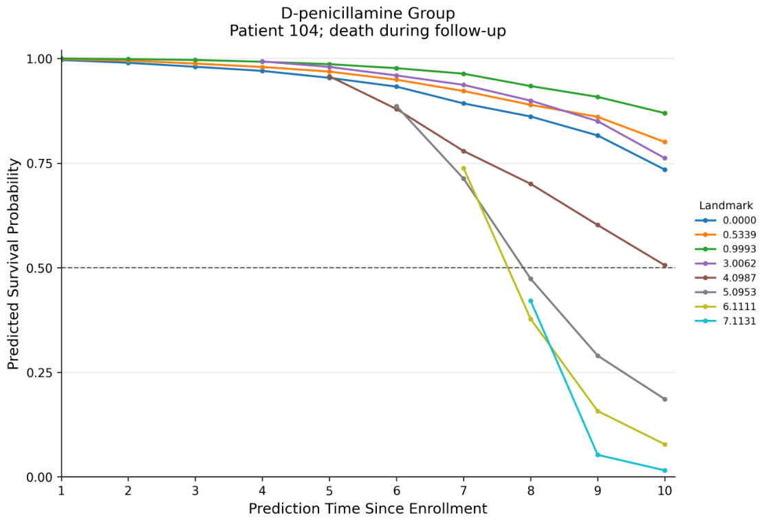
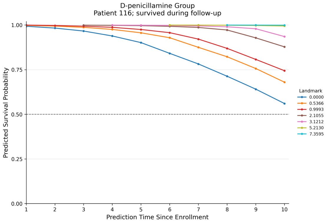
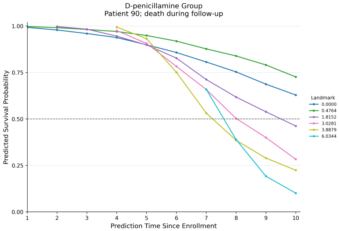
Three representative patients were selected from the PBC data to illustrate the dynamically predicted survival-probability curves generated by TCN-DCM. Patient 116 received D-penicillamine and remained alive throughout follow-up; Patients 104 and 90 also received D-penicillamine but died during follow-up. Figure 2, Figure 3 and Figure 4 show their dynamically predicted survival-probability curves at different observation times. Each curve corresponds to a prediction made at a particular observation time and incorporates only the longitudinal covariate information observed up to and including that time.

As follow-up information for Patient 116 accumulated, the model produced increasingly stable predictions. Based on baseline information at year 0, the model estimated a probability of death before year 9 exceeding 40%. After information at years 0.54 and 1.00 was incorporated under D-penicillamine treatment, the predicted mortality risk decreased substantially, with the estimated probability of death before year 9 falling below 25%. Predictions based on longitudinal information from years 2.11–7.36 showed a further decline and gradual stabilization of the predicted mortality risk.

Patient 104 showed a different dynamic pattern. The model produced relatively high predicted survival probabilities early in follow-up, but the curves shifted downward as new information was incorporated. Based on measurements from baseline through year 3.00, TCN-DCM did not identify the patient as being at high risk of death. As additional longitudinal information accumulated, the predicted survival curves declined progressively. After information at year 5.10 was incorporated, the model estimated an approximately 50% probability of death before year 8. Predictions based on measurements at years 6.11 and 7.11 indicated a further increase in estimated mortality risk.

For Patient 90, who also received D-penicillamine, the model produced a dynamic pattern similar to that of Patient 104, indicating a gradual increase in mortality risk over time.

Overall, the dynamic prediction results for these three patients demonstrate that the TCN-DCM model can continuously update individual survival probability estimates by integrating longitudinal covariate histories observed up to different time points. This provides a time-adaptive framework for individualized risk assessment during clinical follow-up.

5. Discussion

In this study, we proposed the TCN-DCM dynamic prediction model for longitudinal survival data. The model incorporates repeatedly observed covariate information and captures the temporal variation in time-varying covariates, enabling more comprehensive feature extraction for survival prediction. By combining temporal convolutional networks with the Deep Cox Mixtures framework, the proposed model provides a data-driven approach for dynamic survival prediction while relaxing the global PH assumption through latent risk components. Therefore, it retains a connection with classical survival analysis while improving the flexibility of risk modeling for longitudinal data.

The simulation experiments and real-data case analysis showed that TCN-DCM achieved robust predictive performance regardless of whether the PH assumption held or was violated. Further parameter-sensitivity, internal-ablation, random-initialization, and robustness analyses under varying sample sizes, censoring rates, and missing rates showed that TCN-DCM generally maintained stable $C^{\mathrm{td}}$, AUC, and BS performance under the prespecified experimental conditions. MCEM optimization also exhibited a high proportion of valid training histories and consistent convergence characteristics. Although some model components and parameter values produced modest performance changes, the main conclusions were consistent across experimental settings, supporting the numerical stability and predictive robustness of the proposed model. The individualized dynamic prediction analysis further illustrated how predicted survival probabilities were updated as longitudinal follow-up information accumulated, demonstrating the model’s ability to support time-updated individualized risk assessment. These results suggest that the proposed method can provide statistical support for identifying adverse-event risk and adapting risk-intervention strategies in medicine, engineering, economics, and related fields.

References

1. Diggle, P.J.; Heagerty, P.J.; Liang, K.Y.; Zeger, S.L. Analysis of Longitudinal Data; Oxford University Press: Oxford, UK, 2002. [Google Scholar]
2. Asgari, S.; Khalili, D.; Zayeri, F.; Azizi, F.; Hadaegh, F. Dynamic Prediction Models Improved the Risk Classification of Type 2 Diabetes Compared with Classical Static Models. J. Clin. Epidemiol. 2021, 140, 33–43. [Google Scholar] [CrossRef]
3. Achakzai, M.A.K.; Peng, J. Detecting Financial Statement Fraud Using Dynamic Ensemble Machine Learning. Int. Rev. Financ. Anal. 2023, 89, 102827. [Google Scholar] [CrossRef]
4. Wulfsohn, M.S.; Tsiatis, A.A. A Joint Model for Survival and Longitudinal Data Measured with Error. Biometrics 1997, 53, 330–339. [Google Scholar] [CrossRef]
5. van Houwelingen, H.C. Dynamic Prediction by Landmarking in Event History Analysis. Scand. J. Stat. 2007, 34, 70–85. [Google Scholar] [CrossRef]
6. Lee, C.; Yoon, J.; van der Schaar, M. Dynamic-DeepHit: A Deep Learning Approach for Dynamic Survival Analysis With Competing Risks Based on Longitudinal Data. IEEE Trans. Biomed. Eng. 2020, 67, 122–133. [Google Scholar] [CrossRef] [PubMed]
7. Howle, L.E.; Weber, P.W.; Nichols, J.M. Bayesian Approach to Decompression Sickness Model Parameter Estimation. Comput. Biol. Med. 2017, 82, 3–11. [Google Scholar] [CrossRef] [PubMed]
8. Andrinopoulou, E.R.; Nasserinejad, K.; Szczesniak, R.; Rizopoulos, D. Integrating Latent Classes in the Bayesian Shared Parameter Joint Model of Longitudinal and Survival Outcomes. Stat. Methods Med. Res. 2020, 29, 3294–3307. [Google Scholar] [CrossRef] [PubMed]
9. Rizopoulos, D.; Molenberghs, G.; Lesaffre, E.M.E.H. Dynamic Predictions with Time-Dependent Covariates in Survival Analysis Using Joint Modeling and Landmarking. Biom. J. 2017, 59, 1261–1276. [Google Scholar] [CrossRef] [PubMed]
10. Rizopoulos, D.; Taylor, J.M.G. Optimizing Dynamic Predictions from Joint Models Using Super Learning. Stat. Med. 2024, 43, 1315–1328. [Google Scholar] [CrossRef] [PubMed]
11. Nagpal, C.; Li, X.; Dubrawski, A. Deep Survival Machines: Fully Parametric Survival Regression and Representation Learning for Censored Data With Competing Risks. IEEE J. Biomed. Health Inform. 2021, 25, 3163–3175. [Google Scholar] [CrossRef] [PubMed]
12. Nagpal, C.; Jeanselme, V.; Dubrawski, A. Deep Parametric Time-to-Event Regression with Time-Varying Covariates. In Proceedings of Machine Learning Research, Proceedings of the AAAI Spring Symposium on Survival Prediction—Algorithms, Challenges, and Applications, Stanford University, Palo Alto, CA, USA, 22–24 March 2021; PMLR: Cambridge, MA, USA, 2021; Volume 146, pp. 184–193. [Google Scholar]
13. Zeng, L.; Zhang, J.; Chen, W.; Ding, Y. tdCoxSNN: Time-Dependent Cox Survival Neural Network for Continuous-Time Dynamic Prediction. J. R. Stat. Soc. Ser. C Appl. Stat. 2025, 74, 187–203. [Google Scholar] [CrossRef] [PubMed]
14. Mesinovic, M.; Watkinson, P.; Zhu, T. DySurv: Dynamic Deep Learning Model for Survival Analysis with Conditional Variational Inference. J. Am. Med. Inform. Assoc. 2026, 33, 112–122. [Google Scholar] [CrossRef] [PubMed]
15. Nagpal, C.; Yadlowsky, S.; Rostamzadeh, N.; Heller, K. Deep Cox Mixtures for Survival Regression. In Proceedings of Machine Learning Research, Proceedings of the 6th Machine Learning for Healthcare Conference, Virtual Event, 6–7 August 2021; PMLR: Cambridge, MA, USA, 2021; Volume 149, pp. 674–708. [Google Scholar]
16. Dempster, A.P.; Laird, N.M.; Rubin, D.B. Maximum Likelihood from Incomplete Data via the EM Algorithm. J. R. Stat. Soc. Ser. B Stat. Methodol. 1977, 39, 1–22. [Google Scholar] [CrossRef]
17. Wei, G.C.G.; Tanner, M.A. A Monte Carlo Implementation of the EM Algorithm and the Poor Man’s Data Augmentation Algorithms. J. Am. Stat. Assoc. 1990, 85, 699–704. [Google Scholar] [CrossRef]
18. Kingma, D.P.; Welling, M. Auto-Encoding Variational Bayes. In Proceedings of the 2nd International Conference on Learning Representations, Banff, AB, Canada, 14–16 April 2014. [Google Scholar]
19. Pickett, K.L.; Suresh, K.; Campbell, K.R.; Davis, S.; Juarez-Colunga, E. Random Survival Forests for Dynamic Predictions of a Time-to-Event Outcome Using a Longitudinal Biomarker. BMC Med. Res. Methodol. 2021, 21, 216. [Google Scholar] [CrossRef] [PubMed]
20. Gerds, T.A.; Kattan, M.W.; Schumacher, M.; Yu, C. Estimating a Time-Dependent Concordance Index for Survival Prediction Models with Covariate Dependent Censoring. Stat. Med. 2013, 32, 2173–2184. [Google Scholar] [CrossRef] [PubMed]
21. Hung, H.; Chiang, C.T. Optimal Composite Markers for Time-Dependent Receiver Operating Characteristic Curves with Censored Survival Data. Scand. J. Stat. 2010, 37, 664–679. [Google Scholar] [CrossRef]
22. Rustand, D.; van Niekerk, J.; Krainski, E.T.; Rue, H.; Proust-Lima, C. Fast and Flexible Inference for Joint Models of Multivariate Longitudinal and Survival Data Using Integrated Nested Laplace Approximations. Biostatistics 2024, 25, 429–448. [Google Scholar] [CrossRef] [PubMed]
23. Dickson, E.R.; Grambsch, P.M.; Fleming, T.R.; Fisher, L.D.; Langworthy, A. Prognosis in Primary Biliary Cirrhosis: Model for Decision Making. Hepatology 1989, 10, 1–7. [Google Scholar] [CrossRef] [PubMed]
Figure 1. Temporal convolutional network Deep Cox Mixtures model.
Mathematics 14 02727 g001
Figure 2. Dynamically predicted survival-probability curves for Patient 116 in the D-penicillamine group. Patient 116 remained alive during follow-up.
Mathematics 14 02727 g002
Figure 3. Dynamically predicted survival-probability curves for Patient 104 in the D-penicillamine group. Patient 104 died during follow-up.
Mathematics 14 02727 g003
Figure 4. Dynamically predicted survival-probability curves for Patient 90 in the D-penicillamine group. Patient 90 died during follow-up.
Mathematics 14 02727 g004