HBI-Net: Hierarchical Bitemporal Interaction Network for Directional Algal Bloom Change Detection in Multispectral Imagery

Abstract

Satellite remote sensing constitutes a critical methodology for monitoring algal bloom dynamics in eutrophic lakes. However, the majority of existing research predominantly emphasizes single-date extraction or area-based statistics, thereby offering limited pixel-level characterization of bloom appearance and disappearance. These two phenomena bear distinct implications for water quality management: Bloom appearance indicates potential water-quality risks, whereas bloom disappearance often reflects the effectiveness of management interventions or natural decay processes. In this study, we conceptualize bloom monitoring as a directional change-detection problem and introduce the Algal Bloom Change Detection (ABCD) dataset, which comprises 5038 bitemporal Sentinel-2 multispectral image patches from Lake Taihu and Lake Chaohu, annotated into three categories: unchanged, bloom appearance, and bloom disappearance. Furthermore, we propose the Hierarchical Bitemporal Interaction Network (HBI-Net), which integrates a shared Swin-T backbone, a Hierarchical Bitemporal Interaction Block (HBI Block), and a Spatial-Channel Decoder (SC-Decoder). The HBI Block employs signed-temporal-difference gating to maintain change directionality across multiple scales, while the SC-Decoder performs spatial-channel recalibration prior to three-class classification. Experimental results on the ABCD dataset demonstrate that HBI-Net achieves a mean Intersection over Union (mIoU) of 88.08%, outperforming all compared methods; ablation studies further validate the contributions of both the HBI Block and the SC-Decoder. Additionally, when evaluated on the S2Looking building change-detection dataset, HBI-Net attains the highest mIoU, suggesting its potential applicability across different domains.

1. Introduction

Algal bloom outbreaks represent one of the most common environmental hazards in eutrophic lakes, posing significant threats to aquatic ecosystem stability and adversely affecting fisheries, tourism, and other water-dependent economic activities. Consequently, satellite-based monitoring of algal blooms has emerged as a fundamental approach in the management of aquatic environments [1,2].

In algal-bloom monitoring, existing remote sensing studies mainly focus on single-date bloom extraction or time-series area statistics, characterizing bloom presence and temporal variations in total bloom area [3,4,5]. Although these studies have advanced satellite-based bloom monitoring, they provide limited pixel-level characterizations of where blooms appear or disappear between two dates. Newly appearing bloom regions may indicate increasing water-quality risks and require timely warnings, whereas disappearing regions indicate bloom retreat that may result from natural decay, hydrodynamic transport, meteorological variation, or management intervention. Therefore, monitoring bloom dynamics requires not only estimating changes in total area but also locating bloom appearance and disappearance at the pixel level.

Remote sensing change detection provides a natural framework for identifying spatial changes between two observations [6]. However, existing benchmarks and methods predominantly address buildings, disaster damage, and land-cover changes, for which their targets generally exhibit relatively stable geometries and comparatively well-defined semantic boundaries [7,8,9]. These assumptions do not directly transfer to algal blooms, which occur in dynamic aquatic environments and exhibit fragmented shapes, weak boundaries, and spectral ambiguities associated with turbidity, sun glint, and low-density bloom–water transitions [10,11]. Consequently, automatically distinguishing bloom appearance and disappearance between two dates remains an insufficiently explored problem in satellite-based bloom monitoring.

Directional algal-bloom change detection presents two major challenges. First, bloom appearance and disappearance represent opposite state transitions but may exhibit similar spatial patterns and magnitudes of spectral change [12]. A model that primarily captures change magnitude may therefore localize changed pixels while confusing their change directions. Accordingly, bitemporal feature interaction should preserve the temporal order from $T_1$ to $T_2$ and explicitly model direction-aware dependencies rather than treating the two observations as an unordered pair. Second, genuine bloom changes are typically sparse and occur against dynamic water backgrounds. Suspended sediments, high-turbidity water, sun glint, residual floating algae, and mixed bloom–water pixels can produce reflectance responses similar to those associated with true bloom changes. Meanwhile, fragmented bloom patches, irregular boundaries, and weak bloom–water contrast further increase the risk of missed detections and directional misclassification. An effective model must therefore preserve ordered bitemporal evidence while suppressing background-induced responses.

To address these challenges, we have developed the Algal Bloom Change Detection (ABCD) dataset and proposed the Hierarchical Bitemporal Interaction Network (HBI-Net). Utilizing bitemporal Sentinel-2 multispectral imagery, HBI-Net predicts three pixel-level bloom-change states: unchanged, bloom appearance, and bloom disappearance. At the overall level, HBI-Net is designed to learn multi-scale spatial–spectral contexts to effectively handle fragmented bloom patches, irregular boundaries, and low-contrast bloom–water transitions, thereby providing a more robust representation for directional bloom change predictions. The network employs a shared Swin-T backbone to extract multi-scale spatial–spectral features from the two temporal instances, incorporates HBI Blocks to facilitate hierarchical bitemporal interaction while preserving the signed temporal order, and utilizes a signed-difference fusion neck followed by the SC-Decoder to recalibrate directional change features. Specifically, this architecture addresses two critical issues: The HBI Blocks preserve the temporal order from $T_1$ to $T_2$ and enhance direction-aware feature interaction to distinguish bloom appearance from bloom disappearance, whereas the SC-Decoder recalibrates spatial and channel responses to suppress interference from bloom-like water backgrounds. The principal contributions of this work are summarized as follows:

(1)

To facilitate pixel-level detection of directional changes in bloom occurrences, we constructed the ABCD dataset using data from two representative eutrophic lakes, Lake Taihu and Lake Chaohu. This dataset includes three-class annotations categorizing areas as unchanged, bloom appearance, or bloom disappearance.

(2)

We propose the Hierarchical Bitemporal Interaction Block (HBI Block) to preserve temporal directionality during multi-scale feature learning. Integrated within the shared Swin-T backbone, this block employs signed-temporal-difference gating to strengthen direction-aware representations of bloom appearance and disappearance.

(3)

The Spatial-Channel Decoder (SC-Decoder) is designed to mitigate bloom-like interference from water backgrounds. It recalibrates multi-scale directional change features across spatial and channel dimensions, thereby enhancing the recognition of bloom appearance and disappearance in complex aquatic environments.

2. Related Work

2.1. Remote Sensing Change Detection

Remote sensing change detection seeks to identify surface changes between bitemporal images of the same region and has been extensively applied in urban expansion analysis, disaster assessment, land-cover updating, and ecological monitoring. Early approaches relied on hand-crafted techniques, including image differencing, ratioing, change-vector analysis, and threshold segmentation. While these methods are straightforward and interpretable, they are susceptible to radiometric variations, registration errors, imaging conditions, and the selection of thresholds.

With the advancement of deep learning, convolutional neural networks (CNNs), Siamese networks, U-Net-based architectures, and densely connected designs have been extensively employed for bitemporal change feature extraction and fusion. Methods such as FC-EF, FC-Siam-conc, FC-Siam-diff [6], and SNUNet [13] improve change-region recognition through techniques including input-level fusion, shared encoding, feature differencing, and multi-scale decoding. Furthermore, IFN [14] and SiamCRNN [15] investigate the incorporation of deep supervision and recurrent structures. More recently, Transformers and state-space models have been introduced into change-detection frameworks to effectively capture long-range dependencies, global context, and efficient sequence relationships. Representative approaches in this domain include BIT-R18/BIT [16], ChangeFormer [17], ScratchFormer [18], DMINet [19], and ChangeMamba [20].

Recent baseline studies have advanced change detection by addressing complementary aspects. ChangerEx and Changer focus on feature interactions between bitemporal representations [21]; BTC reevaluates and refines established remote sensing change-detection methodologies [22]; BAN investigates the adaptation of foundation models for change detection [23]; MaskCD-Swin-B/MaskCD conceptualizes change detection through a mask-classification framework [24]. Collectively, these approaches encompass the principal model categories examined in this study, including Siamese CNNs, Transformer-based architectures, state-space models, foundation-model-based techniques, and mask-classification strategies. Siamese hierarchical Transformer architectures have been explored for bitemporal remote-sensing damage assessment. For instance, Da et al. [25] proposed SDAFormer, which employs shared Transformer branches for pre- and post-disaster images to leverage correlations between paired images for building localization and damage classification. Recent studies have also highlighted the importance of preserving subtle task-relevant changes in remote sensing change detection while mitigating irrelevant variations, including clouds, shadows, seasonal effects, and noise [26].

Existing change-detection methodologies are well established for bitemporal remote sensing analysis, with prevalent datasets and applications focusing on buildings, roads, disaster damage, and land cover. Representative datasets such as LEVIR-CD [7] and xBD [8] employ binary annotations indicating changed or unchanged regions and have become standard benchmarks for change-region localization. However, lake algal blooms occur within dynamic aquatic environments characterized by indistinct boundaries, fragmented patches, and complex spectral signatures. Consequently, detecting the appearance and disappearance of blooms in multispectral imagery necessitates a directional change-detection approach specifically designed for water-body scenes.

2.2. Algal Bloom Detection in Remote Sensing

Satellite remote sensing provides extensive spatial coverage, frequent revisit intervals, and long-term continuous observation, establishing itself as a crucial tool for monitoring algal blooms and managing aquatic environments [1,2]. Traditional remote sensing approaches to bloom monitoring mainly include spectral-index mapping, threshold-based detection, and water-quality parameter inversion. Spectral-index and threshold-based methods use the characteristic responses of blooms in the visible, red-edge, NIR, and SWIR bands to identify bloom regions in single-date imagery, whereas inversion models estimate indicators such as chlorophyll-a concentrations to characterize bloom distribution and intensity [10,27].

Spectral-index and threshold-based methods retain clear physical interpretability but are susceptible to water-background variations, suspended sediments, turbidity, sun glint, cloud shadows, and changes in imaging conditions. Their decision rules therefore often require recalibration across lakes, seasons, or sensors [11]. Building on single-date observations, satellite time-series analyses use multi-temporal imagery to characterize bloom occurrence frequency, duration, coverage, outbreak intensity, and interannual variability, thereby supporting long-term monitoring and risk assessment [3,4].

More recently, deep learning methods have been applied to algal-bloom detection and water-body remote sensing. By learning complex spatial–spectral representations, these methods improve bloom segmentation under heterogeneous aquatic backgrounds and reduce reliance on fixed thresholds. Compared with conventional index-based approaches, deep models can integrate texture, spatial context, and multi-band information to recognize bloom patches with irregular shapes, indistinct boundaries, or weak spectral responses [5,28]. Their primary outputs, however, are generally bloom segmentation maps for individual dates, whereas time-series studies more commonly summarize changes in bloom area, occurrence frequency, or outbreak intensity at the regional scale.

Several studies have begun to exploit temporal information more explicitly. Ahn et al. [29] constructed multi-period inputs from pre-bloom and during-bloom PlanetScope observations to improve binary mappings of bloom distribution during a bloom period. Using denser hourly GOCI observations, Wang et al. [30] classified pixel-scale diurnal bloom trajectories as decreasing, decrease-then-increase, increasing, or increase-then-decrease. These studies demonstrate the value of temporal context; however, they focus on current-state bloom mapping or within-day trajectory characterization rather than on a bitemporal semantic transition map that jointly labels bloom appearance and disappearance.

This distinction is important because arbitrary observations from two dates may contain simultaneous local appearance and disappearance even when their total bloom areas are similar. A current-state bloom map does not separately label these two opposite transitions, while dense trajectory analysis requires multiple observations and targets temporal evolution rather than the semantic transition between two selected dates. Bloom appearance generally indicates an expansion of the spatial extent of water-quality risk, whereas bloom disappearance may be associated with natural decay, hydrodynamic transport, meteorological variation, or management intervention. Monitoring bloom dynamics, therefore, requires not only locating changed regions but also preserving the temporal order of bitemporal observations to distinguish non-bloom-to-bloom transitions from bloom-to-non-bloom transitions at the pixel level.

2.3. Directional and Semantic Change Detection

Traditional binary change-detection methods classify each pixel as either changed or unchanged. However, many practical applications require not only the identification of change occurrence but also the determination of its direction or semantic category. For instance, urban building analysis differentiates between construction and demolition, which represent two opposite change directions, while land-cover analysis often involves identifying transitions between different classes. Consequently, directional and semantic change detection have emerged as significant advancements in remote sensing change detection. BCTDNet [12] introduces the JINAN-MCD three-class dataset for buildings in Jinan, where pixels are labeled as unchanged, newly constructed, or demolished. This approach explicitly models the opposing directions of construction and demolition using a SAM-based vision foundation model with attribute-aware decoding. Furthermore, SECOND [9] extends this framework by organizing semantic transitions among multiple land-cover classes into a from–to labeling scheme, thereby enabling more fine-grained directional semantic change detection.

Directional or semantic change detection provides more detailed information compared to binary change detection; however, it also demands more rigorous annotation protocols, precise class definitions, and sophisticated feature modeling. Models are required not only to identify regions of change but also to comprehend the state relationships preceding and following the change. Simple fusion methods such as concatenation, subtraction, or unsigned difference applied at later stages often diminish the temporal ordering between dates, thereby impairing directional discrimination [21].

Applied studies in aquatic and wetland environments can be categorized based on the transition information conveyed by their labels. Using bitemporal Sentinel-2 observations, Wieland and Martinis [31] mapped constant water, water loss, water gain, and invalid observations during the 2018 drought in Germany. From a comprehensive Landsat time series, Pickens et al. [32] further distinguished permanent water and stable seasonal water from gain, loss, dry-period, wet-period, and high-frequency transition states. At a more detailed semantic level, Pan et al. [33] employed bitemporal semantic reasoning to identify wetland changes in Dongting Lake, including water loss and transitions from water to vegetation and mudflat, while Qian et al. [34] developed a temporal–spectral–semantic-aware network for multi-class tidal-wetland change detection. At a broader spatial and temporal scale, Nagel et al. [35] differentiated surface-water advance and recession and recorded the timing of these transitions across rivers, lakes, reservoirs, and other water bodies.

Collectively, these studies demonstrate that aquatic change analysis has advanced beyond simple binary change localization to include explicit directional or from–to semantics. However, their class definitions primarily describe changes in open-water extent, shoreline position, or transitions among water, vegetation, mudflat, and other land-cover categories. Bloom appearance and disappearance differ in that both states occur within persistent water bodies and generally do not alter water extent or land-cover classification. Bloom patches also exhibit irregular morphologies, indistinct boundaries, and complex multispectral responses, and their local changes can be obscured by turbidity, residual floating algae, and water-background variability. Therefore, direct pixel-level mapping of bloom appearance and disappearance from arbitrary bitemporal multispectral image pairs remains comparatively underexplored and requires a dedicated dataset and labeling scheme that preserve the temporal direction from $T_1$ to $T_2$.

3. Study Area and Data Description

3.1. Study Area

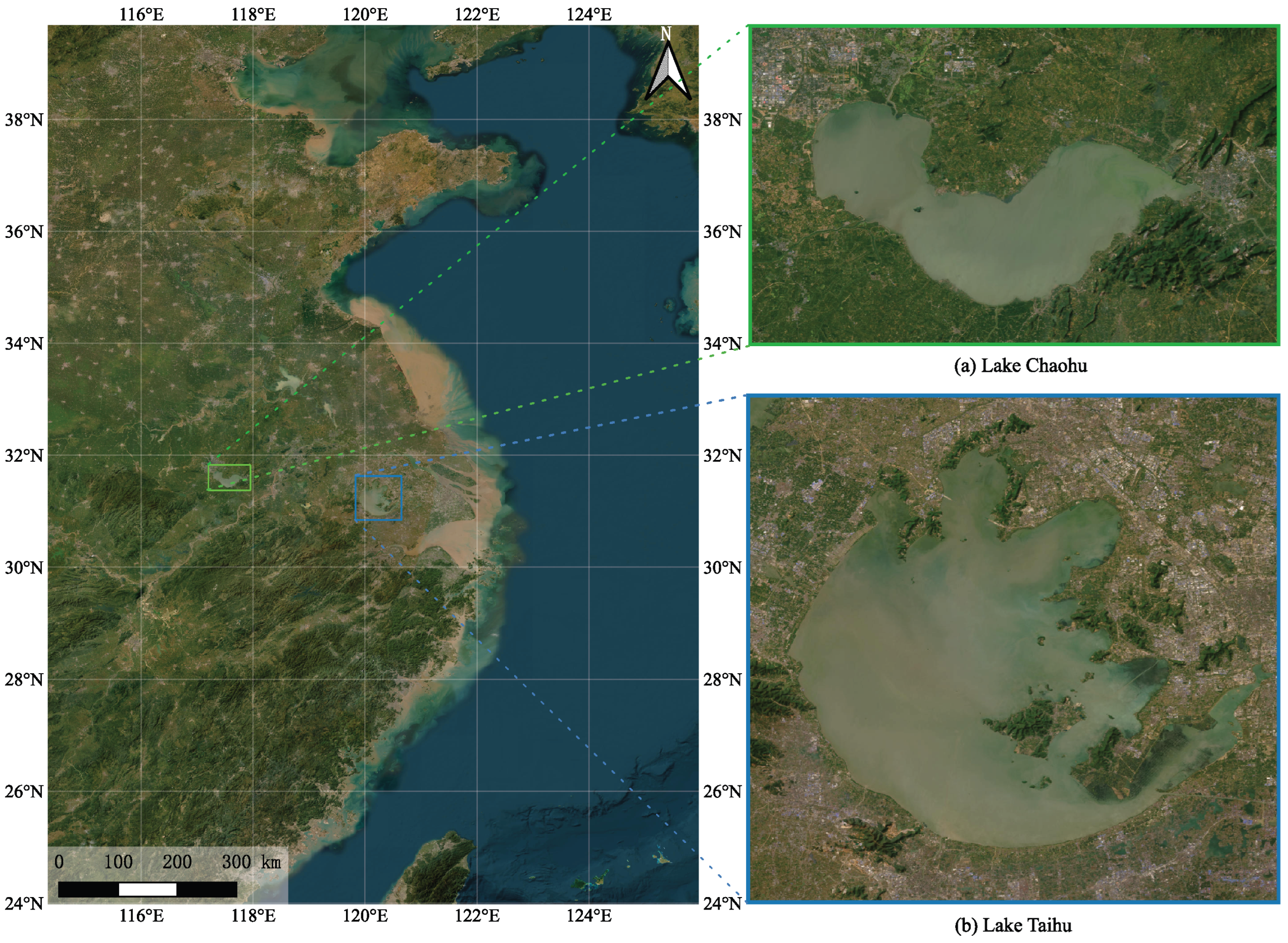
Two representative shallow eutrophic lakes in eastern China, Lake Taihu and Lake Chaohu, were selected as study sites. These lakes differ in terms of watershed development intensity, hydrological characteristics, water exchange dynamics, and bloom development patterns. Collectively, they offer observational samples encompassing frequent bloom outbreaks and urban lake eutrophication. Their geographical locations are illustrated in Figure 1.

Lake Taihu is situated in the central region of the Yangtze River Delta, straddling the boundary between southern Jiangsu Province and northern Zhejiang Province. It represents a typical large, shallow, eutrophic lake in China. The lake’s geographic and morphometric characteristics are detailed in

Table 1. Basic information of the study areas.

Lake	Coordinates	Area (km2)	Mean Depth (m)	Main Bloom-Prone Area
Lake Taihu	$30°{55}^{\prime }$–$31°{33}^{\prime }$ N; $119°{53}^{\prime }$–$120°{36}^{\prime }$ E	2338	1.9	Meiliang Bay, Zhushan Bay, and western shoreline
Lake Chaohu	$31°{25}^{\prime }$–$31°{43}^{\prime }$ N; $117°{16}^{\prime }$–$117°{52}^{\prime }$ E	770	3.0	Western lake region, especially the northwestern shoreline

. Its watershed encompasses the industrial corridor extending across Suzhou, Wuxi, and Changzhou, as well as adjacent densely populated urban areas, which have historically been subjected to combined inputs from industrial wastewater, agricultural runoff, and domestic sewage. Algal blooms predominantly occur during the summer and autumn seasons, exhibiting significant interannual and seasonal variability [36,37].

Lake Chaohu, situated in central Anhui Province, is a significant urban lake adjacent to the city of Hefei. Its geographic and morphometric characteristics are detailed in Table 1. The lake is fed by multiple inflowing rivers, including the Nanfei, Shiwuli, and Pai Rivers, among others, and it connects to the Yangtze River system via the Yuxi River. Due to the rapid expansion of the Hefei metropolitan area, agricultural non-point source pollution, and nutrient inputs from the watershed, Lake Chaohu has remained eutrophic over recent decades, with algal bloom occurrences becoming notably more frequent during the summer and autumn seasons [38,39].

Lake Taihu and Lake Chaohu collectively exemplify representative bloom dynamics observed in shallow eutrophic lakes of eastern China. Variations in lake morphology, watershed pressures, and bloom development between these two lakes enhance the diversity of scenarios within the dataset, thereby facilitating the evaluation of directional change detection across differing lacustrine conditions. The fundamental characteristics of the two lakes are summarized in Table 1.

3.2. Data Acquisition and Dataset Construction

This study utilizes imagery obtained from the Sentinel-2 Multispectral Instrument (MSI) as the primary remote sensing data source. The Sentinel-2 mission [40,41], operated by the twin satellites Sentinel-2A and Sentinel-2B, offers high spatial resolutions, frequent revisit intervals, and multispectral observations encompassing visible, red-edge, NIR, and SWIR bands. These characteristics render the mission particularly suitable for the spatial identification and temporal monitoring of algal blooms in inland lakes. All imagery employed in this study was processed and exported via the Google Earth Engine (GEE) platform [42].

Model inputs were constructed using the Sentinel-2 MSI Level-2A surface reflectance collection (COPERNICUS/S2_SR_HARMONIZED) available on Google Earth Engine. The inputs comprised ten Sentinel-2 reflectance bands (B2, B3, B4, B5, B6, B7, B8, B8A, B11, and B12), with bands B1 and B9 excluded from the network’s input. Band B10 was not considered as an input candidate because it is not included in the Level-2A surface reflectance collection. Due to the varying native spatial resolutions among the bands, all input bands were resampled to a 10 m grid using Google Earth Engine’s default reprojection settings. No additional local resampling was performed thereafter, thereby preserving spatial consistency between the two acquisition dates.

The Sentinel-2 imagery selected for this study covers the period from October 2017 to December 2025, with specific acquisition dates detailed in

Table 2. Selected Sentinel-2 acquisition dates used for ABCD construction.

Lake	Selected Acquisition Dates
Lake Taihu	2019-05-09; 2019-06-03; 2019-08-17; 2019-10-31; 2020-05-03; 2020-07-22; 2020-08-11; 2021-01-13; 2021-01-18; 2021-02-07; 2021-06-22; 2021-09-30; 2021-10-30; 2021-12-29; 2022-02-27; 2022-08-11; 2022-12-24; 2023-01-18; 2023-01-28; 2023-03-04; 2024-01-13; 2024-01-23; 2024-02-12; 2024-03-03; 2024-08-30; 2024-10-29; 2025-01-27; 2025-03-08
Lake Chaohu	2017-10-09; 2019-01-17; 2019-07-11; 2019-09-29; 2019-10-19; 2019-10-24; 2021-09-23; 2021-12-17; 2023-01-31; 2023-02-15; 2023-02-20; 2023-12-27; 2025-01-10; 2025-12-26

. For both Lake Taihu and Lake Chaohu, images were manually chosen based on criteria of low cloud cover and comprehensive coverage of the primary lake area. To facilitate the three-class directional classification task, paired dates were selected to ensure the representation of both appearance and disappearance regions within the dataset. The selection process emphasized image pairs that provided complete observations of the lake interiors while minimizing contamination from clouds and cloud shadows.

Table 2 presents the Sentinel-2 acquisition dates utilized in the construction of ABCD. The number of retained dates varies between the two lakes due to differences in cloud cover, the completeness of the main lake body, and the clarity of the bloom’s spatial distribution.

During preprocessing, persistent main-lake regions were extracted from the JRC Global Surface Water occurrence layer using a 90% occurrence threshold. The resulting water boundary was eroded inward by 30 m to reduce shoreline mixed pixels and minimize interference from near-shore submerged vegetation. For Lake Taihu, the East Taihu region (120.35–120.60° E, 30.95–31.30° N) was additionally excluded because submerged macrophytes and aquaculture installations dominate this area. At the acquisition level, SCL classes 3 (cloud shadow), 8 (medium-probability cloud), 9 (high-probability cloud), and 10 (cirrus) were treated as invalid.

Acquisition-level SCL statistics were computed once for each of the 42 distinct Sentinel-2 acquisitions used in the dataset, including 28 acquisitions for Lake Taihu and 14 for Lake Chaohu. SCL-invalid areas were measured at the native 20 m SCL resolution and converted to 10 m model-grid pixel equivalents. No-data observations were handled separately and excluded from the denominator used to calculate the SCL-invalid percentages.

Table 3. Quantitative summary of spatial lake-region screening and acquisition-level SCL screening.

Lake	Retained Effective Area (km2; % of Candidate Area)	SCL-Invalid Observations Removed (10 m Equivalents; % of Observed)
Lake Taihu	1953.293; 89.781%	6,214,824; 1.137%
Lake Chaohu	736.124; 98.930%	330,078; 0.321%

reports the retained effective lake regions and the invalid observations removed by SCL screening.

Following the preparation of bitemporal image pairs, each pair was partitioned into non-overlapping patches of size $256\times 256$. These patches were subsequently screened based on the proportion of valid water pixels and the distribution of directional change pixels. Each retained sample comprises multispectral image patches from the two time points, accompanied by the corresponding pixel-level directional change annotations. The resulting ABCD dataset consists of 5038 bitemporal patches derived from 41 source scene pairs. To prevent data leakage between neighboring patches across subsets, all patches originating from the same source scene pair were assigned to the same subset. The 41 source scene pairs were divided into 29 for training, six for validation, and six for testing, yielding 3296, 787, and 955 patches, respectively. A public preview release and dataset documentation are available on GitHub at https://github.com/abie9068/ABCD-Dataset/releases/tag/ABCD-Dataset (accessed on 18 July 2026).

3.3. Directional Change Label Generation

Algal blooms undergo rapid changes, possess diffuse boundaries, and display irregular spatial morphology, rendering large-scale pixel-level annotation based on field observations impractical. Therefore, we generate a single-date bloom reference mask for each Sentinel-2 image and derive directional change labels by combining the masks from time points $T_1$ and $T_2$.

The single-date bloom reference mask is derived from the Floating Algae Index (FAI) [10]. The FAI quantifies the extent to which the near-infrared reflectance of a pixel deviates from a spectral baseline, which is linearly interpolated between the red and shortwave-infrared bands. This deviation is pronounced for surfaces affected by cyanobacterial blooms and minimal for typical water bodies:

$$\mathrm{FAI}=R_{\mathrm{NIR}}-R_{\mathrm{NIR}}^{\prime },R_{\mathrm{NIR}}^{\prime }=R_{\mathrm{RED}}+(R_{\mathrm{SWIR}}-R_{\mathrm{RED}})·{\displaystyle \frac{{\lambda }_{\mathrm{NIR}}-{\lambda }_{\mathrm{RED}}}{{\lambda }_{\mathrm{SWIR}}-{\lambda }_{\mathrm{RED}}}},$$

(1)

where $R_{\mathrm{RED}}$, $R_{\mathrm{NIR}}$, and $R_{\mathrm{SWIR}}$ are the surface reflectances of Sentinel-2 bands B4 (665 nm), B8 (842 nm), and B11 (1610 nm), respectively, and ${\lambda }_{\mathrm{RED}}$, ${\lambda }_{\mathrm{NIR}}$, and ${\lambda }_{\mathrm{SWIR}}$ are the corresponding band-center wavelengths.

A fixed FAI cutoff does not consistently distinguish bloom from non-bloom areas across different acquisitions. This inconsistency arises because the FAI distribution varies between scenes due to factors such as acquisition date, residual atmospheric correction errors, suspended sediment, and bloom density. Consequently, applying a global threshold tends to result in over-extraction on certain dates and under-extraction on others. To address this issue, the threshold is determined individually for each scene through visual supervision. Specifically, the FAI map of each acquisition is binarized at uniform increments of 0.005 within the range $[-0.02,0.10]$, generating 25 candidate bloom masks per scene. These candidates are then examined sequentially from the lowest to the highest threshold by comparing them against the B8/B4/B3 false-color composite and the FAI map. The threshold corresponding to the mask that most accurately aligns with the visually identifiable bloom region is selected as the operational threshold for that scene.

GEE was used to generate the FAI maps, SCL-screened valid-water masks, and candidate threshold masks. These layers were exported and overlaid in QGIS, a free and open-source desktop GIS application, along with the B8/B4/B3 false-color composites. Two annotators experienced in interpreting bloom imagery from Lake Taihu and Lake Chaohu independently inspected the candidate masks and manually corrected weak boundaries, fragmented bloom patches, and residual high-reflectance non-bloom regions in QGIS. Their per-scene masks were subsequently reconciled to produce a consensus single-date bloom reference. The corrected single-date masks were then combined programmatically to generate the directional labels. The FAI maps, candidate threshold masks, and valid-water masks were used solely for label generation and quality control and were not incorporated into model training or inference.

Given the bloom reference masks at times $T_1$ and $T_2$, directional change labels are generated by combining the bloom and non-bloom states at these two time points for each pixel. Specifically, a pixel classified as non-bloom at $T_1$ and bloom at $T_2$ is labeled as bloom appearance; conversely, a pixel classified as bloom at $T_1$ and non-bloom at $T_2$ is labeled as bloom disappearance. If the states at both times are identical, the pixel is labeled as unchanged. These label definitions are summarized in

Table 4. Directional change label definition.

${\mathit{T}}_1$ State	${\mathit{T}}_2$ State	Label
non-bloom	non-bloom	unchanged
bloom	bloom	unchanged
non-bloom	bloom	bloom appearance
bloom	non-bloom	bloom disappearance

.

For subsequent visualizations, bitemporal images are presented using the B8/B4/B3 false-color composite to enhance the visual discrimination of bloom-rich regions; however, model training and inference continue to utilize the 10-band reflectance imagery.

4. Methodology

This section introduces the proposed HBI-Net, a network designed for detecting directional bloom changes in bitemporal Sentinel-2 multispectral imagery. The network effectively localizes regions of bloom change and differentiates between bloom appearance and bloom disappearance.

4.1. Overall Architecture of HBI-Net

Let $I^{T_1}$ and $I^{T_2}$ represent the Sentinel-2 multispectral images of an identical region acquired at two distinct dates, $T_1$ and $T_2$. Following spatial co-registration, these images can be expressed as

$$I^{T_1},I^{T_2}\in {\mathbb{R}}^{H\times W\times C}.$$

(2)

The model utilizes co-registered bitemporal multispectral imagery as input and generates a pixel-wise directional change label map as the output:

$$Y\in {\{0,1,2\}}^{H\times W}.$$

(3)

Here, the value 0 indicates no change, 1 represents the appearance of bloom, and 2 signifies the disappearance of bloom. Regions deemed invalid are excluded from both training and evaluation processes by applying a valid-pixel mask. Unlike binary change detection, this task maintains temporal directionality in addition to localizing changes: a transition from non-bloom at time $T_1$ to bloom at time $T_2$ is classified as bloom appearance, whereas a transition from bloom at $T_1$ to non-bloom at $T_2$ is classified as bloom disappearance.

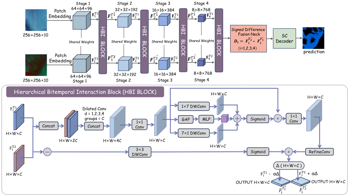
As illustrated in the upper part of Figure 2, HBI-Net comprises a shared Swin-T backbone, the HBI Block, a signed-difference fusion neck, and the SC-Decoder. The shared Swin-T backbone initially extracts multi-scale spatial-spectral features from the two temporal images. HBI Blocks, inserted after each of the four encoder stages, facilitate bitemporal directional interaction. Subsequently, the signed-difference fusion neck computes the signed difference $T_2-T_1$ of the interacted paired features, producing multi-scale directional change features. Finally, the SC-Decoder performs spatial and channel recalibration on these features and generates predictions for unchanged areas, bloom appearance, and bloom disappearance. The internal structure of the HBI Block is further detailed in the lower part of Figure 2, enabling a comprehensive understanding of the block-level operations in conjunction with the overall data flow.

Each component addresses a primary challenge: Swin-T captures fragmented boundaries and regional context; the HBI Block maintains directional semantics from $T_1$ to $T_2$; the SC-Decoder emphasizes potential change regions while mitigating interference from water backgrounds. The subsequent subsections discuss these components in the specified order, with Figure 2 providing a structural reference for the HBI Block.

4.2. Shared Swin-T Backbone

4.2.1. Multispectral Input Embedding

Algal blooms display distinct reflectance properties across the visible, red-edge, NIR, and SWIR spectral bands. The Sentinel-2 spectral bands vary in numerical range, noise characteristics, and semantic significance; consequently, directly utilizing raw multispectral channels for subsequent hierarchical feature extraction complicates the learning process. To address this, the shared Swin-T backbone initially applies a multispectral input embedding to each temporal instance $T_j\in \{T_1,T_2\}$. Specifically, the input image $I^{T_j}\in {\mathbb{R}}^{H\times W\times C}$ undergoes per-band normalization, followed by projection through a non-overlapping patch-projection layer (with patch size $4\times 4$ and stride 4) that maps each local spectral cube to a 96-dimensional token. This is subsequently normalized via layer normalization, yielding the shallowest-level embedding feature map for the corresponding date:

$$F_0^{T_j}=\mathrm{PatchEmbed}\left(I^{T_j}\right),T_j\in \{T_1,T_2\}.$$

(4)

Here, PatchEmbed denotes the multispectral input-embedding module, which consists of a $4\times 4$ non-overlapping patch projection followed by layer normalization. The resulting output feature map has a resolution of $H/4\times W/4$, with each token represented by a 96-dimensional vector. The two dates utilize identical embedding parameters, ensuring that $F_0^{T_1}$ and $F_0^{T_2}$ reside within a comparable representation space.

4.2.2. Hierarchical Feature Extraction

Bloom regions exhibit variable shapes and relatively indistinct boundaries; a single image may concurrently contain large floating blooms, small fragmented patches, and regions with weak boundary transitions. Consequently, a single feature scale is insufficient to capture both local details and regional contexts. To address this, the shared Swin-T backbone extracts multi-scale features from both dates after embedding:

$$\{F_i^{T_j}{\}}_{i=1}^4=B(F_0^{T_j}),T_j\in \{T_1,T_2\}.$$

(5)

Here, B represents the shared Swin-T backbone, $i\in \{1,2,3,4\}$ indicates the feature level, and $F_i^{T_j}$ denotes the feature map corresponding to date $T_j$ at the i-th level. The backbone employs parameter sharing across the two dates, enabling the progressive extraction of multi-scale representations that range from shallow details to deep contextual information. This parameter sharing guarantees that $F_i^{T_1}$ and $F_i^{T_2}$ occupy a comparable representation space, thereby providing the paired hierarchical features necessary for the subsequent HBI Block. The output resolutions and channel dimensions for the four levels are $H/4\times W/4\times 96$, $H/8\times W/8\times 192$, $H/16\times W/16\times 384$, and $H/32\times W/32\times 768$.

Hierarchical feature encoding plays a crucial role in directional bloom change detection. Shallow features retain local boundaries, textures, and spectral variations, which are essential for identifying weak bloom signals and boundary-transition regions characterized by small patches and low-contrast textures. In contrast, deep features capture broader regional contexts, facilitating the differentiation of extensive floating blooms from stable water backgrounds. By means of progressive feature abstraction, the shared Swin-T backbone generates a multi-scale representation that evolves from low-level details to high-level semantic information, forming the foundation for the HBI Block.

4.3. Hierarchical Bitemporal Interaction Block (HBI Block)

The appearance and disappearance of blooms may exhibit similar magnitudes of change but occur in opposite temporal sequences. Effective directional discrimination necessitates explicit modeling of temporal order during feature learning; conventional methods such as simple concatenation, subtraction, or unsigned differencing employed as pre-decoder fusion tend to diminish directional semantic information [21]. Consequently, HBI-Net incorporates the HBI Block following each of the four encoder stages to facilitate explicit interactions between paired bitemporal features. As illustrated in the lower part of Figure 2, each HBI Block receives $F_i^{T_1}$ and $F_i^{T_2}$ at the same scale and outputs the updated features $F_i^{T_1^{\prime }}$ and $F_i^{T_2^{\prime }}$.

4.3.1. Paired Temporal Feature Construction

Directional change detection compares states at two dates, using their correspondence to characterize bloom change. Organizing bitemporal features as pairs offers direct change cues to the HBI Block. Specifically, for bitemporal features $F_i^{T_1}$ and $F_i^{T_2}$ at the i-th scale, we create a paired temporal representation via channel-wise concatenation:

$$Z_i=\mathrm{Concat}(F_i^{T_1},F_i^{T_2}).$$

(6)

4.3.2. Direction-Guided Gated Interaction

Paired features must distinguish effective changes from background noise. Bloom appearance and disappearance usually occur in localized areas, with different channels responding variably. The HBI Block combines a context branch and a signed-difference gating branch to generate a residual update:

$$R_i={\varphi }_i\left(Z_i\right),$$

(7)

$$G_i=\sigma \left({\psi }_i(F_i^{T_2}-F_i^{T_1})\right).$$

(8)

Here, $Z_i$ is the paired temporal representation formed by the channel-wise concatenation of $F_i^{T_1}$ and $F_i^{T_2}$ at the i-th scale; $R_i$ is the multi-scale bitemporal context response from the context branch; $G_i$ is the spatial gating response from the signed-difference branch; $\sigma$ denotes the sigmoid activation. Specifically, ${\varphi }_i$ comprises four parallel grouped $3\times 3$ dilated convolution branches [43] with dilation rates of 1, 2, 3, and 4. Since $Z_i$ has $2C$ channels and the grouped convolutions use groups = C, the paired representation is divided into C groups, with each group containing the $T_1$ and $T_2$ responses of the same semantic channel. Each branch outputs a C-channel feature map; the four branch outputs are then concatenated into a $4C$-channel representation and projected by a $1\times 1$ mixing convolution. This is followed by a channel-axial context block and a refinement convolution consisting of a depthwise $3\times 3$ convolution and a $1\times 1$ convolution. The channel-axial context block mixes channels and applies horizontal and vertical depthwise convolutions to capture row- and column-direction context. The multi-dilation design enables $R_i$ to capture bloom patches, weak boundary transitions, and stripe-shaped water structures of varying sizes at the same scale, providing candidate context responses for the gated update.

${\psi }_i$ includes a depthwise $3\times 3$ convolution and batch normalization, taking the signed temporal difference $F_i^{T_2}-F_i^{T_1}$ as input to produce a direction-aware gate $G_i$ [44]. Unlike the unsigned difference, which only measures change magnitude, the signed difference retains the direction from $T_1$ to $T_2$. Compared to simple bitemporal concatenation, it directly links gating weights to directional response. Thus, the context branch provides updatable multi-scale responses, while the signed-difference gating branch controls the spatial strength of these responses in the directional residual update.

Given the context response and signed-difference gate, the model generates the directional residual term and updates the two-date features:

$${\Delta }_i=R_i\odot G_i,$$

(9)

$$F_i^{T_1^{\prime }}=F_i^{T_1}-{\alpha }_i{\Delta }_i,F_i^{T_2^{\prime }}=F_i^{T_2}+{\alpha }_i{\Delta }_i.$$

(10)

Here, ⊙ denotes element-wise multiplication, and ${\alpha }_i$ is a learnable residual scaling coefficient initialized to 0.1. This initialization limits residual magnitude early in training to stabilize optimization and enables the model to adaptively amplify updates as it converges. The update is applied with opposite signs to the two dates, preserving the temporal order of $F_i^{T_1}$ and $F_i^{T_2}$ during interactions.

4.3.3. Signed Directional Difference Representation

After bitemporal interactions via the HBI Block, features encode change-relevant context. Since distinguishing bloom appearance from disappearance depends on the order from $T_1$ to $T_2$, the signed-difference fusion neck arranges the bitemporal features into an explicit directional change representation:

$$D_i=F_i^{T_2^{\prime }}-F_i^{T_1^{\prime }}.$$

(11)

The difference feature $D_i$ is computed from the bitemporal features after the HBI Block update, capturing both the temporal direction from $T_1$ to $T_2$ and the context-enhanced representation at the i-th scale. Substituting the HBI residual update yields an equivalent decomposition:

$$D_i=\left(F_i^{T_2}-F_i^{T_1}\right)+2{\alpha }_i{\Delta }_i,$$

(12)

The directional difference equals the original signed temporal difference plus twice the gated cross-temporal residual; the factor of 2 results from the symmetric opposite-sign updates to $F_i^{T_1}$ and $F_i^{T_2}$. By preserving temporal order, it offers clearer cues to distinguish bloom appearance from disappearance.

4.4. Spatial-Channel Decoder (SC-Decoder)

Given the multi-scale directional change feature ${\left\{D_i\right\}}_{i=1}^4$ from the signed-difference fusion neck, HBI-Net employs the SC-Decoder to generate pixel-wise directional change predictions. Since multi-scale features include irrelevant responses from stable water backgrounds, turbidity differences, illumination changes, and weak boundaries, directly fusing them would introduce noise into the predictions. Thus, the SC-Decoder recalibrates these features along both channel and spatial dimensions.

4.4.1. Multi-Scale Feature Alignment

The multi-scale directional change features from the signed-difference fusion neck vary in channel count and spatial resolution across levels. To ensure stable multi-level fusion, the decoder projects each scale’s features to a unified channel dimension and upsamples them to the finest encoder stage’s common spatial resolution $H/4\times W/4$:

$$U_i={\mathrm{Up}}_i({\eta }_i\left(D_i\right)).$$

(13)

Here, ${\eta }_i(·)$ represents the channel-projection mapping for the i-th scale, and ${\mathrm{Up}}_i(·)$ denotes the upsampling operation. Features from different scales are concatenated along the channel dimension:

$$Q=\mathrm{Concat}(U_1,U_2,U_3,U_4).$$

(14)

4.4.2. Spatial-Channel Recalibration

The aligned multi-scale change features still include irrelevant responses from stable water backgrounds and turbidity gradients, with different spectral–semantic channels contributing variably to directional bloom change. For clarity, we express channel and spatial recalibration on the fused feature Q:

$$M_c=\sigma (g_c\left(\mathrm{GAP}\left(Q\right)\right)),$$

(15)

$$M_s=\sigma (g_s\left(Q\right)),$$

(16)

$$\widehat{Q}=Q\odot M_c\odot M_s.$$

(17)

Here, $M_c$ and $M_s$ represent the channel and spatial attention weights, respectively; $\mathrm{GAP}(·)$ denotes global average pooling, while $g_c(·)$ and $g_s(·)$ are the channel and spatial recalibration functions.

Channel recalibration selects spectral–semantic responses relevant to directional bloom changes while suppressing irrelevant channels. Spatial recalibration emphasizes potential change regions and reduces large stable water backgrounds.

The recalibration equations above offer a simplified single-feature perspective. In practice, the SC-Decoder employs channel- and spatial-attention mechanisms from CBAM [45] and SE-Net [46] within a UPer [47] decoding path. Each lateral feature is projected to a unified channel dimension and recalibrated, while the PSP top feature is also recalibrated before top–down FPN fusion. Since the decoder input is the multi-scale directional change feature $D_i$ from the signed-difference fusion neck, this recalibration enhances bloom appearance and disappearance regions and suppresses stable water backgrounds.

4.4.3. Prediction and Training Objective

After spatial-channel recalibration, the feature $\widehat{Q}$ integrates multi-scale change information, enhancing potential change regions and channel responses. It is mapped to three-class logits at the decoder resolution and then upsampled to the original image resolution:

$$\begin{array}{cc}\hfill \tilde{O}& =\chi \left(\widehat{Q}\right),\tilde{O}\in {\mathbb{R}}^{H/4\times W/4\times 3},\hfill \\ \hfill O& ={\mathrm{Up}}_{4\times }\left(\tilde{O}\right),O\in {\mathbb{R}}^{H\times W\times 3}.\hfill \end{array}$$

(18)

Here, $\chi (·)$ denotes the final classification mapping at the decoder resolution, and ${\mathrm{Up}}_{4\times }(·)$ denotes bilinear upsampling by a factor of 4. Per-pixel probabilities for the three classes are obtained using softmax:

$$P=\mathrm{softmax}\left(O\right).$$

(19)

Each pixel is assigned the class with the highest probability. Training uses per-pixel three-class supervision, excluding invalid regions from the loss. Dice loss [48] serves as the training objective; details are provided in the experimental section.

$$\Omega =\{n\mid n \mathrm{is} \mathrm{used} \mathrm{for} \mathrm{supervision}\},$$

(20)

$${\mathcal{L}}_{\mathrm{Dice}}=1-{\displaystyle \frac{1}{3}}{\displaystyle \sum _{k=0}^2}{\displaystyle \frac{2{\sum }_{n\in \Omega }{p}_{n,k}{y}_{n,k}+ϵ}{{\sum }_{n\in \Omega }{p}_{n,k}+{\sum }_{n\in \Omega }{y}_{n,k}+ϵ}}.$$

(21)

Here, $\Omega$ denotes the set of valid supervised pixels, $p_{n,k}$ is the predicted probability that pixel n belongs to class k, $y_{n,k}\in \{0,1\}$ is the corresponding one-hot label, and $ϵ$ is a smoothing term preventing division by zero. The Dice loss weights the three classes equally, mitigating the dominance of the abundant unchanged class and ensuring equal optimization weights for bloom appearance and disappearance.

5. Experiments

The experiments are organized around three research questions: (1) Does HBI-Net improve the balanced recognition of unchanged areas, bloom appearance, and bloom disappearance compared with representative change-detection methods on ABCD? (2) How do the Swin-T backbone, HBI Block, and SC-Decoder contribute progressively to directional bloom change detection under the successive ablation settings? (3) Does the proposed architecture remain effective in a non-bloom directional change-detection scenario on S2Looking? To answer these questions, we compare HBI-Net with representative methods on ABCD, analyze its class-wise performance and computational cost, conduct a progressive ablation study, and evaluate its cross-domain applicability on S2Looking. All experiments on ABCD adhere to the input setup, train/validation/test split, and evaluation protocol defined in the dataset section.

5.1. Experimental Settings

5.1.1. Evaluation Metrics

We use mean Intersection over Union (mIoU), mean F-score (mFscore), mean precision (mPrecision), mean recall (mRecall), overall accuracy (OA), and class-wise IoU as evaluation metrics. Let C denote the number of classes; here, $C=3$. For class c, ${\mathrm{TP}}_c$, ${\mathrm{FP}}_c$, and ${\mathrm{FN}}_c$ represent the numbers of true-positive, false-positive, and false-negative pixels, respectively, and N is the total number of valid pixels used in the evaluation. The metrics are defined as follows:

$${\mathrm{IoU}}_c={\displaystyle \frac{{\mathrm{TP}}_c}{{\mathrm{TP}}_c+{\mathrm{FP}}_c+{\mathrm{FN}}_c}},$$

(22)

$$\mathrm{mIoU}={\displaystyle \frac{1}{C}}{\displaystyle \sum _{c=0}^{C-1}}{\mathrm{IoU}}_c,$$

(23)

$$P_c={\displaystyle \frac{{\mathrm{TP}}_c}{{\mathrm{TP}}_c+{\mathrm{FP}}_c}},R_c={\displaystyle \frac{{\mathrm{TP}}_c}{{\mathrm{TP}}_c+{\mathrm{FN}}_c}},$$

(24)

$$\mathrm{mPrecision}={\displaystyle \frac{1}{C}}{\displaystyle \sum _{c=0}^{C-1}}{P}_c,\mathrm{mRecall}={\displaystyle \frac{1}{C}}{\displaystyle \sum _{c=0}^{C-1}}{R}_c,$$

(25)

$$\mathrm{F}{1}_c={\displaystyle \frac{2P_c{R}_c}{P_c+R_c}},\mathrm{mFscore}={\displaystyle \frac{1}{C}}{\displaystyle \sum _{c=0}^{C-1}}\mathrm{F}{1}_c,$$

(26)

$$\mathrm{OA}={\displaystyle \frac{{\sum }_{c=0}^{C-1}{\mathrm{TP}}_c}{N}}.$$

(27)

We use mean Intersection over Union (mIoU) as the primary metric to evaluate balanced performance across the three classes. Class-wise IoU is employed to analyze the recognition of unchanged, appearance, and disappearance categories separately. Overall accuracy (OA) reports the overall correctness rate across all valid pixels, while mean precision (mPrecision), mean recall (mRecall), and mean F-score (mFscore) characterize the precision, completeness, and balance of the predicted regions, respectively.

5.1.2. Implementation and Training Settings

All ABCD experiments are implemented in PyTorch (2.4.1), utilizing MMEngine, MMSegmentation [49], and Open-CD [50]. They are trained and tested on a single NVIDIA GeForce RTX 4090 GPU. HBI-Net employs the bitemporal input setup described in the dataset section. Inputs are normalized using per-band mean and standard deviation statistics computed from the training set, and the same normalization parameters are applied to both $T_1$ and $T_2$.

Unless otherwise stated, all compared methods are trained and evaluated using the same protocol. The detailed training settings are summarized in

Table 5. Training settings used for all compared methods.

Item	Setting
Optimizer	AdamW [51]
Initial learning rate	6 × 10−5
Minimum learning rate	1 × 10−6
Weight decay	0.01
Batch size	8
Total iterations	20,000
Learning-rate schedule	1000-iteration linear warm-up followed by cosine annealing
Data augmentation	Random rotation, random cropping, horizontal flipping, and vertical flipping
Training loss	Three-class Dice loss
Validation interval	Every 2000 iterations
Checkpoint selection	Highest validation mIoU

.

AdamW was selected because it combines parameter-wise adaptive updates, as in Adam, with decoupled weight decay, allowing weight decay to act directly on the model parameters rather than being scaled by adaptive learning rates [51]. Compared to Adam with conventional L2 regularization, this formulation provides more consistent control over parameter regularization. Additionally, compared to SGD, the adaptive first- and second-moment estimates of AdamW facilitate the joint optimization of heterogeneous components in HBI-Net, including the Swin-T backbone, HBI Blocks, and SC-Decoder. Therefore, AdamW was used in conjunction with linear warm-up and cosine annealing throughout the experiments.

5.2. Comparison with Existing Methods on ABCD

5.2.1. Quantitative Results

Table 6. Quantitative comparison on the ABCD test set.

Method	mIoU	mFscore	mPrec.	mRec.	OA	Unch. IoU	App. IoU	Disapp. IoU
FC-Siam-conc	84.97	91.83	92.65	91.07	93.17	89.93	82.64	82.33
SNUNet	84.45	91.53	90.67	92.50	92.72	89.06	83.29	81.00
BIT-R18	82.27	90.20	94.33	87.04	92.15	88.86	80.08	77.88
ChangeFormer	84.35	91.48	89.56	93.78	92.54	88.61	82.19	82.24
ChangerEx	83.85	91.18	89.36	93.34	92.29	88.28	81.89	81.37
ChangeMamba	83.71	91.10	89.71	92.68	92.28	88.35	81.17	81.61
BTC	86.65	92.82	91.64	94.21	93.80	90.56	84.90	84.49
BAN	83.40	90.91	89.95	91.95	92.18	88.29	80.82	81.08
MaskCD-Swin-B	82.44	90.34	88.22	93.17	91.45	86.95	78.70	81.66
HBI-Net	88.08	93.64	93.65	93.63	94.61	91.89	85.86	86.47

The best results are highlighted in bold and underlined. Rows are organized by method family rather than by score. “Unch.,” “App.,” and “Disapp.” denote unchanged, bloom appearance, and bloom disappearance, respectively.

compares HBI-Net with representative change-detection methods from the main model families discussed above. The baselines include Siamese CNNs and nested U-Nets (FC-Siam-conc [6] and SNUNet [13]); Transformer-based methods (BIT-R18/BIT [16] and ChangeFormer [17]; feature-interaction and state-space baselines (ChangerEx/Changer [21] and ChangeMamba [20]); and recent optimized, foundation-model-based, and mask-classification methods (BTC [22], BAN [23], and MaskCD-Swin-B/MaskCD [24]). Collectively, these baselines span the principal architectural paradigms in remote sensing change detection, from classical Siamese CNNs to recent Transformer, state-space, foundation-model-based, and mask-classification frameworks. The table follows this method–family order, with HBI-Net listed last. HBI-Net achieves the highest scores on three overall metrics, mIoU (88.08), mFscore (93.64), and OA (94.61), while attaining the second-highest mPrecision of 93.65. Although BIT-R18 obtains a higher mPrecision, its mRecall and mIoU are considerably lower; in contrast, HBI-Net maintains a more balanced precision–recall profile, resulting in the best mFscore and mIoU. Compared with the second-best method, HBI-Net improves mIoU by 1.43 and mFscore by approximately 0.82.

The comparison highlights the role of temporal ordering in ABCD. Existing baselines mainly emphasize the spatial localization of changed regions, and their fusion operations often convert bitemporal differences into magnitude-oriented change responses. In ABCD, bloom appearance and bloom disappearance are two opposite transitions between water and bloom states. Similar spatial extents and reflectance contrasts can therefore correspond to different labels depending on the order from $T_1$ to $T_2$. HBI-Net embeds this order into feature learning through signed temporal differences. The signed-difference gate conditions feature interaction on the direction of $F_i^{T_2}-F_i^{T_1}$, and the signed fusion neck carries this directional evidence to the decoder. This mechanism links the improvement in mIoU and mFscore to a more balanced recognition of the two minority directional classes, while OA is less sensitive because unchanged water dominates the pixel distribution.

At the class level, HBI-Net achieves IoU scores of 91.89, 85.86, and 86.47 for unchanged, appearance, and disappearance classes, respectively, which are the highest values reported in the table. Compared to the second-best results, HBI-Net improves IoU by 1.33, 0.96, and 1.98 for these three classes, with the largest gain observed in the disappearance class. This class-wise pattern is consistent with the imaging characteristics of algal blooms. Appearance usually corresponds to a water-to-bloom transition that introduces stronger NIR and red-edge responses, whereas disappearance often corresponds to a bloom-to-water transition in which residual floating algae, turbidity, and low-contrast boundary mixtures may still remain. Therefore, disappearance is more likely to be confused with weak stable-water variations or partially decayed bloom signals. The larger improvement on this class indicates that HBI-Net captures transition directions more reliably while detecting changed regions. Mechanistically, the signed-difference gate makes the residual interaction depend on the sign of $F_i^{T_2}-F_i^{T_1}$, and the subsequent signed-difference fusion retains this order when producing directional change features. The SC-Decoder then recalibrates these features spatially and spectrally, suppressing extensive unchanged water while emphasizing channels and locations associated with bloom-to-water and water-to-bloom transitions.

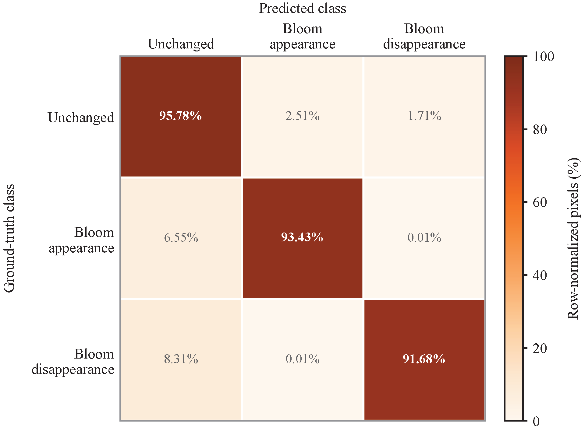
The row-normalized confusion matrix in Figure 3 provides a complementary view of the class-wise error distribution. HBI-Net correctly recognizes 95.78%, 93.43%, and 91.68% of ground-truth unchanged, appearance, and disappearance pixels, respectively. The main errors occur when appearance and disappearance pixels are predicted as unchanged (6.55% and 8.31%, respectively), whereas direct confusion between the two opposite directional classes is only 0.01% in either direction. This pattern indicates that the remaining difficulty lies primarily in the detection of weak or boundary-level changes rather than reversal of the temporal direction.

5.2.2. Model Complexity and Inference Efficiency

To evaluate computational cost and inference efficiency, we report the parameter count, FLOPs, and FPS using the same input configuration and hardware. The results are summarized in

Table 7. Model complexity and inference efficiency comparison on ABCD, listed in the same method–family order as Table 6.

Method	Params	FLOPs	FPS
FC-Siam-conc	1.549 M	5.122 G	262.07
SNUNet	3.013 M	11.866 G	178.91
BIT-R18	2.992 M	8.817 G	89.79
ChangeFormer	25.008 M	10.246 G	37.78
ChangerEx	3.468 M	1.831 G	58.13
ChangeMamba	32.62 M	20.652 G	28.40
BTC	58.953 M	67.432 G	39.30
BAN	68.895 M	29.303 G	30.19
MaskCD-Swin-B	107.28 M	52.155 G	6.45
HBI-Net	64.159 M	68.43 G	30.47

. Classical CNN-based baselines have relatively simple architectures and achieve higher FPS, but their ABCD accuracy is lower than that of recent methods. Transformer-, Mamba-, and attention-enhanced models generally require greater computational resources in exchange for stronger feature representations. HBI-Net has 64.159 million parameters and 68.43 billion FLOPs, and it runs at 30.47 FPS. This speed is comparable to recent high-capacity models, and it is significantly faster than the most computationally intensive mask-classification baseline. Combined with the accuracy results in Table 6, HBI-Net achieves the highest mIoU while maintaining an acceptable inference cost.

The complexity results clarify how the model capacity is used. HBI-Net has fewer parameters than BAN and MaskCD-Swin-B, yet it obtains higher accuracy; it is also much faster than MaskCD-Swin-B. The additional computation is concentrated on hierarchical bitemporal interaction and spatial-channel recalibration, both of which correspond directly to the two principal difficulties of ABCD: directional ambiguity and water-background interference. From an engineering perspective, this is a targeted allocation of capacity. The shared backbone keeps the two temporal branches in a common feature space, and the interaction block modifies paired features through lightweight directional residual updates. This trade-off is important for operational lake monitoring, where large-area and repeated temporal observations require a model that improves directional reliability without making inference prohibitively expensive.

5.2.3. Qualitative Results

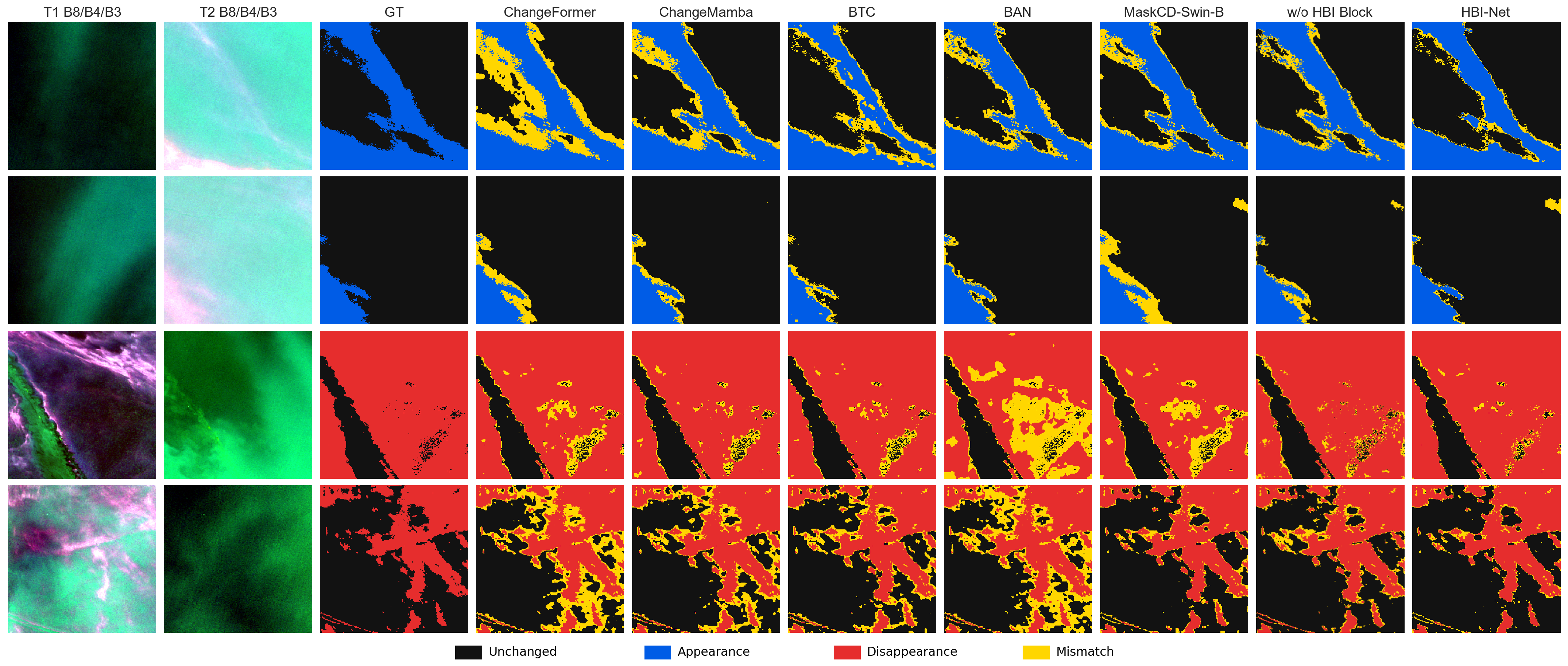
Figure 4 presents a qualitative comparison on the ABCD test set. $T_1$ and $T_2$ are displayed using a B8/B4/B3 false-color composite. Predictions are visualized with three semantic colors, and prediction–ground truth mismatches are highlighted in yellow. In addition to representative existing methods, the two rightmost prediction columns show the same samples without the HBI Block and with the complete HBI-Net, respectively. This paired, ablation-aligned output comparison makes the effect of hierarchical bitemporal interaction directly observable in the final directional predictions. Relative to the variant without the HBI Block, HBI-Net produces fewer yellow mismatch pixels, reduces fragmented predictions and large-scale missed detections, and more closely follows the appearance and disappearance regions in the ground truth.

These visual results correspond to different error mechanisms. Fragmented false detections usually occur when a model responds to local spectral contrast without sufficient spatial context, whereas missed detections occur when sparse bloom patches are overwhelmed by the dominant unchanged-water background. Directional errors arise when the model recognizes that a change has occurred but fails to preserve the temporal order of that change. HBI-Net addresses these three failure modes through different parts of the architecture. The hierarchical Swin-T backbone and the multi-dilation context branch provide regional context for bloom patches with variable sizes; the signed gate prevents the same contextual response from being applied symmetrically to appearance and disappearance; the SC-Decoder suppresses broad stable-water responses before classification. In particular, the output differences between the two rightmost columns are consistent with the quantitative HBI Block ablation results presented in

Table 8. Ablation results on ABCD.

Ablation Setting	mIoU	mFscore	OA	Unch. IoU	App. IoU	Disapp. IoU
ResNet-50 backbone	82.66	90.44	92.21	88.82	79.84	79.31
Swin-T backbone	86.65	92.82	93.80	90.56	84.90	84.49
+HBI Block	87.15	93.11	94.12	91.12	85.04	85.30
+SC-Decoder (HBI-Net)	88.08	93.64	94.61	91.89	85.86	86.47

The best results are highlighted in bold and underlined. Unch., App., and Disapp. denote unchanged, bloom appearance, and bloom disappearance, respectively.

. After introducing hierarchical bitemporal interaction, the predicted regions contain fewer mismatched pixels and better preserve the direction of the transition. Therefore, this side-by-side comparison provides qualitative evidence that complements the numerical ablation findings.

5.3. Ablation Study

To analyze the contribution of each component, we conducted an ablation study; the results are reported in Table 8. The “ResNet-50 backbone” setting uses ResNet-50 [52] as the encoder, while the “Swin-T backbone” setting replaces the encoder with Swin-T [53], a comparably sized hierarchical Transformer backbone, to assess the impact of hierarchical Transformer features on directional bloom change detection. The HBI Block and the SC-Decoder are then added sequentially to evaluate the contributions of hierarchical bitemporal interaction and spatial-channel decoding.

Replacing ResNet-50 with Swin-T increases mIoU from 82.66 to 86.65 and improves appearance and disappearance IoU by 5.06 and 5.18, respectively. This large improvement indicates that the first requirement of directional bloom change detection is a sufficiently strong spatial–spectral representation. Algal blooms have irregular boundaries, fragmented distributions, and scale-varying shapes; a purely convolutional encoder tends to rely on progressively enlarged local receptive fields, whereas the hierarchical shifted-window attention of Swin-T can model wider regional dependencies while preserving multi-scale feature maps. The nearly symmetric improvement on appearance and disappearance also suggests that Swin-T mainly strengthens the common representation needed to detect bloom-related structures before the model explicitly separates their temporal directions.

Adding the HBI Block on top of the Swin-T backbone further raises the mIoU to 87.15, with the disappearance IoU increasing by 0.81. The HBI Block contributes through a direction-consistent interaction rule. The context branch extracts candidate bitemporal responses from paired features, while the signed-difference gate determines where these responses should be injected according to $F_i^{T_2}-F_i^{T_1}$. Because the residual update is added to $T_2$ and subtracted from $T_1$, the resulting feature difference contains both the original temporal contrast and an amplified direction-aware residual. This anti-symmetric update provides a structural explanation for why the HBI Block improves directional classes, particularly disappearance, where the model must distinguish true bloom decay from weak background variations.

Incorporating the SC-Decoder on top results in the full HBI-Net achieving an mIoU of 88.08, which is 0.93 higher than the previous configuration, and it improves the appearance and disappearance IoU by 0.82 and 1.17, respectively. This improvement reflects a third mechanism: After directional features have been formed, the decoder must select reliable evidence from multi-scale features under strong water-background interference. Channel recalibration emphasizes the spectral–semantic channels related to bloom transitions, while spatial recalibration suppresses large unchanged-water regions, turbidity-induced responses, and weak non-bloom reflectance changes. The sequential gains in Table 8 therefore support a layered interpretation of HBI-Net: Swin-T supplies spatial–spectral contexts, the HBI Block encodes ordered temporal interactions, and the SC-Decoder filters the resulting directional evidence before pixel-level classification. The modules are complementary because each one addresses a different stage of the same failure chain.

5.4. Cross-Dataset Evaluation on S2Looking

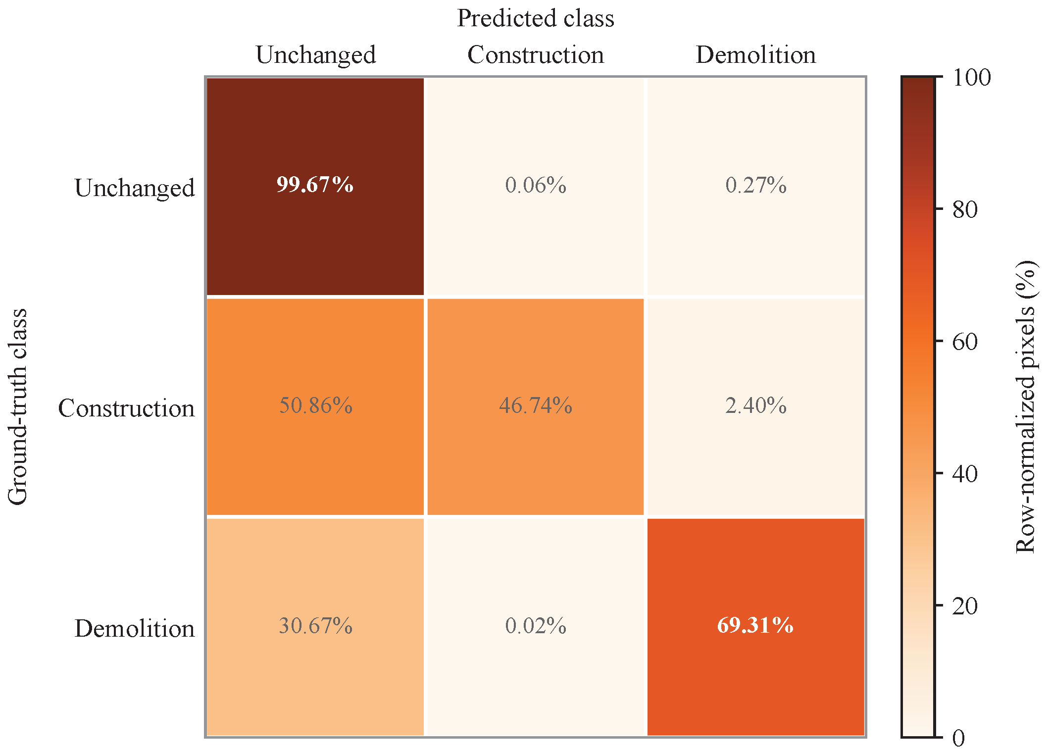
In addition to ABCD, we evaluate HBI-Net on the S2Looking dataset. S2Looking [54] is a large-scale remote sensing dataset for building change detection, containing 5000 high-resolution bitemporal image pairs. Unlike most binary change-detection datasets, S2Looking provides pixel-level annotations for construction and demolition, which we organize into a three-class directional task (unchanged, construction, and demolition), referred to here as S2Looking-building-3class. Building change differs from algal bloom change in spectral signature, morphological structure, and background interference; thus, this experiment tests whether HBI-Net generalizes to a non-bloom directional change-detection scenario.

Table 9. Cross-dataset evaluation on S2Looking-building-3class.

Method	mIoU	OA	Unchanged IoU	Construction IoU	Demolition IoU
FC-Siam-conc	32.94	98.82	98.82	0.00	0.00
SNUNet	38.57	98.77	98.77	2.31	14.63
BIT-R18	50.11	98.98	98.98	19.85	31.50
ChangeFormer	62.25	99.27	99.27	35.13	52.35
ChangerEx	58.78	99.15	99.15	31.67	45.51
ChangeMamba	49.88	98.32	98.32	20.17	31.15
BTC	61.83	99.22	99.21	33.92	52.35
BAN	48.52	99.02	99.01	17.23	29.31
MaskCD-Swin-B	46.54	97.34	97.33	19.52	22.75
HBI-Net	63.33	99.26	99.26	37.04	53.71

The best results are highlighted in bold and underlined. Rows follow the same method–family order as Table 6.

follows the same method–family order as Table 6.

HBI-Net achieves an mIoU of 63.33 on the S2Looking-building-3class dataset, the highest score reported in the table. At the class level, HBI-Net attains IoU scores of 37.04 and 53.71 for construction and demolition, respectively, both outperforming the other methods listed. These results demonstrate that the bitemporal interaction and spatial-channel decoding architecture of HBI-Net effectively generalize to building construction and demolition scenarios, maintaining the ability to distinguish directional change classes.

The significance of this cross-dataset result lies in the difference between the two domains. Buildings and algal blooms differ substantially in spatial resolution, object geometry, spectral characteristics, and background composition. HBI-Net remains competitive on S2Looking because its central inductive bias is more general: Opposite semantic transitions are represented as ordered temporal differences. Construction and demolition are directionally analogous to bloom appearance and disappearance. The improvement on the construction and demolition classes indicates that the model’s generalization comes from directional representation learning, while the high unchanged IoU mainly reflects the class distribution of the dataset.

Figure 5 further reports the row-normalized confusion matrix on the S2Looking-building-3class. The recall values are 99.67%, 46.74%, and 69.31% for unchanged, construction, and demolition, respectively. Most missed construction and demolition pixels are assigned to the unchanged class (50.86% and 30.67%), consistent with the severe pixel-level class imbalance and the small spatial extent of many building changes. By contrast, direct confusion between the two directional change classes remains limited: 2.40% of construction pixels are predicted as demolition, and 0.02% of demolition pixels are predicted as construction. These values complement but are not numerically equivalent to the class IoUs in Table 9, because IoU additionally penalizes false-positive predictions.

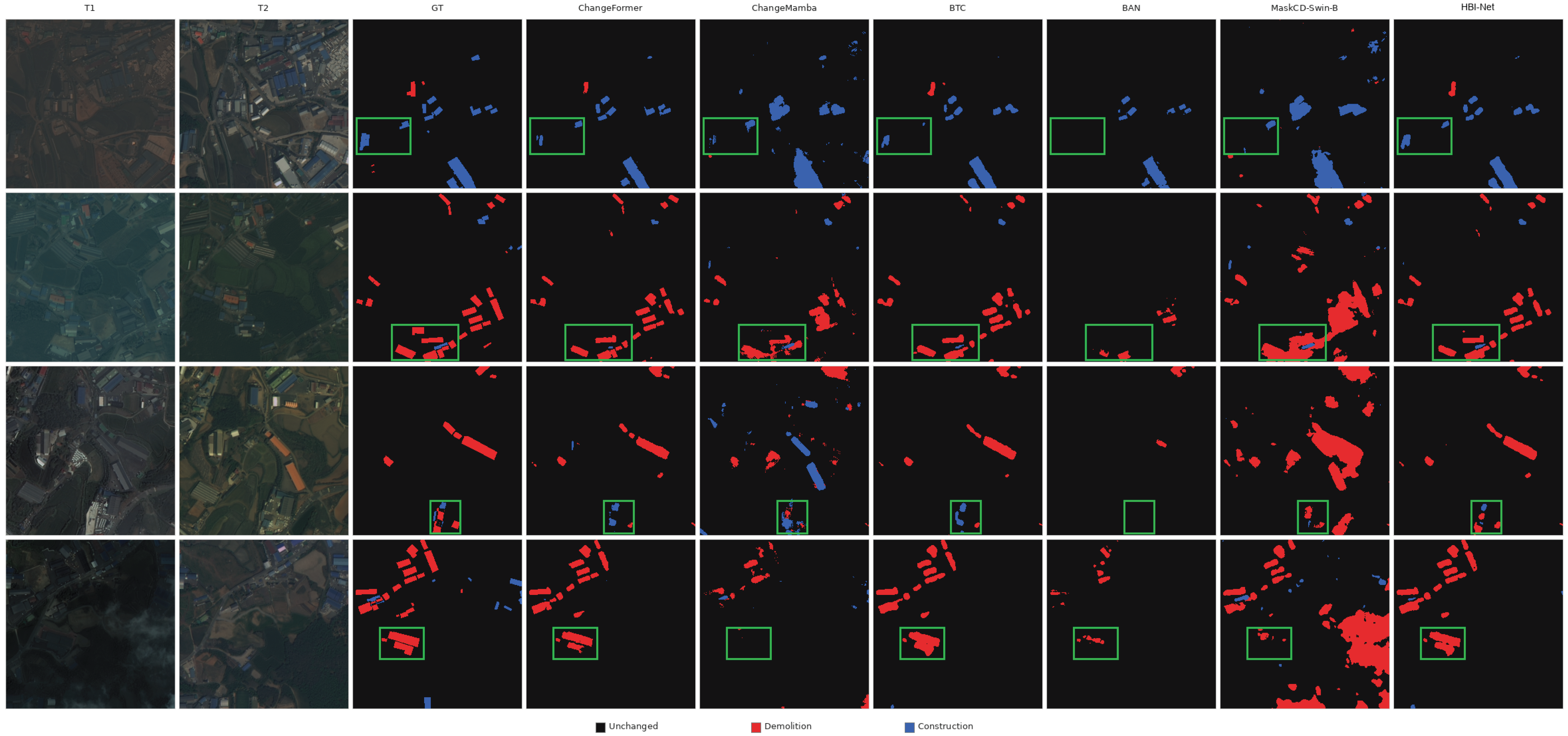
Corresponding qualitative results are presented in Figure 6.

Taken together, these experiments address the three research questions posed at the beginning of this section. The ABCD comparison verifies the overall claim that directional bloom change detection requires a balanced recognition of unchanged, appearance, and disappearance classes under complex aquatic backgrounds. The ablation study explains where the improvement comes from: Hierarchical Transformer features provide spatial–spectral contexts, signed bitemporal interaction preserves temporal order, and spatial-channel recalibration suppresses irrelevant background responses. The S2Looking experiment further shows that the key principle is not limited to algal blooms but applies to directional change-detection tasks in which two change classes represent opposite temporal transitions. Together, these findings indicate that the proposed modules are empirically effective because their mechanisms are aligned with the structure of the task.

6. Conclusions and Future Work

We investigate algal bloom monitoring in eutrophic lakes through the lens of directional change detection. Unlike most previous remote-sensing studies on algal blooms, which primarily focus on single-date bloom extraction, time-series area statistics, or water-quality parameter estimation, we formulate bloom change as a pixel-level, three-class classification task that distinguishes among unchanged areas, bloom appearance, and bloom disappearance. This distinction enables us to differentiate between an increase in the spatial extent of water-quality risk (appearance) and management outcomes or natural decay (disappearance). To support this study, we have developed the ABCD dataset for directional bloom change detection, which includes Sentinel-2 bitemporal multispectral observations of Lake Taihu and Lake Chaohu. Additionally, we propose HBI-Net, which incorporates the HBI Block and the SC-Decoder to jointly model directional differences between paired multispectral images, thereby enhancing the recognition of bloom appearance and disappearance.

On the ABCD dataset, HBI-Net achieves 88.08% mIoU, the highest among the compared change-detection methods. These gains are primarily concentrated on the bloom appearance and bloom disappearance classes and align with the central objective of directional bloom change detection: distinguishing between two semantically opposite change classes. Ablation studies further demonstrate that the Swin-T backbone, the HBI Block, and the SC-Decoder each contribute independently to performance improvements. Additionally, the S2Looking cross-dataset results highlight the method’s potential for cross-domain generalization.

This study has several limitations. In regions with strong turbidity gradients and weak-signal bloom boundaries, the appearance and disappearance of blooms can still be locally misclassified. Moreover, because ABCD currently covers only Lake Taihu and Lake Chaohu, it does not represent the full diversity of lake morphologies, trophic states, and optical regimes. Future work will proceed in three directions. First, ABCD will be extended to additional bloom-prone lakes under different climatic and optical conditions, including Lake Erie, Lake Okeechobee, Lake Winnipeg, and Dianchi Lake. Cross-lake evaluation will be used to assess robustness across various lake morphologies, trophic states, and optical regimes. Second, to improve temporal coverage when cloud-free Sentinel-2 observations are limited, feature-level fusion with complementary Sentinel-1 SAR and Landsat-8/9 optical data will be investigated. Third, boundary-aware loss functions and spatial–morphological priors will be explored to enhance the delineation of weak-signal bloom boundaries. In parallel, weak samples will be addressed through hard-sample mining focused on low-contrast boundary patches and subtle directional changes, combined with targeted spectral–spatial augmentation to reduce local directional confusion and isolated false detections.

References

- Ho, J.C.; Michalak, A.M.; Pahlevan, N. Widespread global increase in intense lake phytoplankton blooms since the 1980s. Nature 2019, 574, 667–670. [Google Scholar] [CrossRef] [PubMed]
- Shen, L.; Xu, H.; Guo, X. Satellite remote sensing of harmful algal blooms (HABs) and a potential synthesized framework. Sensors 2012, 12, 7778–7803. [Google Scholar] [CrossRef] [PubMed]
- Stumpf, R.P.; Wynne, T.T.; Baker, D.B.; Fahnenstiel, G.L. Interannual variability of cyanobacterial blooms in Lake Erie. PLoS ONE 2012, 7, e42444. [Google Scholar] [CrossRef] [PubMed]
- Mishra, S.; Stumpf, R.P.; Schaeffer, B.A.; Werdell, P.J.; Loftin, K.A.; Meredith, A. Measurement of cyanobacterial bloom magnitude using satellite remote sensing. Sci. Rep. 2019, 9, 18310. [Google Scholar] [CrossRef] [PubMed]
- Feng, C.; Wang, S.; Li, Z. Long-term spatial variation of algal blooms extracted using the U-net model from 10 years of GOCI imagery in the East China Sea. J. Environ. Manag. 2022, 321, 115966. [Google Scholar] [CrossRef] [PubMed]
- Daudt, R.C.; Le Saux, B.; Boulch, A. Fully convolutional siamese networks for change detection. In Proceedings of the 2018 25th IEEE International Conference on Image Processing (ICIP); IEEE: New York, NY, USA, 2018; pp. 4063–4067. [Google Scholar] [CrossRef]
- Chen, H.; Shi, Z. A spatial-temporal attention-based method and a new dataset for remote sensing image change detection. Remote Sens. 2020, 12, 1662. [Google Scholar] [CrossRef]
- Gupta, R.; Goodman, B.; Patel, N.; Hosfelt, R.; Sajeev, S.; Heim, E.; Doshi, J.; Lucas, K.; Choset, H.; Gaston, M. Creating xBD: A dataset for assessing building damage from satellite imagery. In Proceedings of the IEEE/CVF Conference on Computer Vision and Pattern Recognition (CVPR) Workshops; IEEE: New York, NY, USA, 2019; pp. 10–17. [Google Scholar]
- Yang, K.; Xia, G.-S.; Liu, Z.; Du, B.; Yang, W.; Pelillo, M.; Zhang, L. Asymmetric siamese networks for semantic change detection in aerial images. IEEE Trans. Geosci. Remote Sens. 2022, 60, 5609818. [Google Scholar] [CrossRef]
- Hu, C. A novel ocean color index to detect floating algae in the global oceans. Remote Sens. Environ. 2009, 113, 2118–2129. [Google Scholar] [CrossRef]
- Garcia, R.A.; Fearns, P.; Keesing, J.K.; Liu, D. Quantification of floating macroalgae blooms using the scaled algae index. J. Geophys. Res. Oceans 2013, 118, 26–42. [Google Scholar] [CrossRef]
- Zhang, W.; Li, J.; Wang, S.; Wan, J. BCTDNet: Building change-type detection networks with the segment anything model in remote sensing images. Remote Sens. 2025, 17, 2742. [Google Scholar] [CrossRef]
- Fang, S.; Li, K.; Shao, J.; Li, Z. SNUNet-CD: A densely connected siamese network for change detection of VHR images. IEEE Geosci. Remote Sens. Lett. 2022, 19, 8007805. [Google Scholar] [CrossRef]
- Zhang, C.; Yue, P.; Tapete, D.; Jiang, L.; Shangguan, B.; Huang, L.; Liu, G. A deeply supervised image fusion network for change detection in high resolution bi-temporal remote sensing images. ISPRS J. Photogramm. Remote Sens. 2020, 166, 183–200. [Google Scholar] [CrossRef]
- Chen, H.; Wu, C.; Du, B.; Zhang, L.; Wang, L. Change detection in multisource VHR images via deep siamese convolutional multiple-layers recurrent neural network. IEEE Trans. Geosci. Remote Sens. 2020, 58, 2848–2864. [Google Scholar] [CrossRef]
- Chen, H.; Qi, Z.; Shi, Z. Remote sensing image change detection with transformers. IEEE Trans. Geosci. Remote Sens. 2022, 60, 5607514. [Google Scholar] [CrossRef]
- Bandara, W.G.C.; Patel, V.M. A transformer-based siamese network for change detection. In Proceedings of the 2022 IEEE International Geoscience and Remote Sensing Symposium; IEEE: New York, NY, USA, 2022; pp. 207–210. [Google Scholar] [CrossRef]
- Noman, M.; Fiaz, M.; Cholakkal, H.; Narayan, S.; Anwer, R.M.; Khan, S.; Khan, F.S. Remote sensing change detection with transformers trained from scratch. IEEE Trans. Geosci. Remote Sens. 2024, 62, 4704214. [Google Scholar] [CrossRef]
- Feng, Y.; Jiang, J.; Xu, H.; Zheng, J. Change detection on remote sensing images using dual-branch multilevel intertemporal network. IEEE Trans. Geosci. Remote Sens. 2023, 61, 4401015. [Google Scholar] [CrossRef]
- Chen, H.; Song, J.; Han, C.; Xia, J.; Yokoya, N. ChangeMamba: Remote sensing change detection with spatiotemporal state space model. IEEE Trans. Geosci. Remote Sens. 2024, 62, 4409720. [Google Scholar] [CrossRef]
- Fang, S.; Li, K.; Li, Z. Changer: Feature interaction is what you need for change detection. IEEE Trans. Geosci. Remote Sens. 2023, 61, 1–11. [Google Scholar] [CrossRef]
- Rolih, B.; Fučka, M.; Wolf, F.; Zajc, L.Č. Be the change you want to see: Revisiting remote sensing change detection practices. IEEE Trans. Geosci. Remote Sens. 2025, 63, 4704811. [Google Scholar] [CrossRef]
- Li, K.; Cao, X.; Meng, D. A new learning paradigm for foundation model-based remote-sensing change detection. IEEE Trans. Geosci. Remote Sens. 2024, 62, 5610112. [Google Scholar] [CrossRef]
- Yu, W.; Zhang, X.; Das, S.; Zhu, X.X.; Ghamisi, P. MaskCD: A remote sensing change detection network based on mask classification. IEEE Trans. Geosci. Remote Sens. 2024, 62, 5631316. [Google Scholar] [CrossRef]
- Da, Y.; Ji, Z.; Zhou, Y. Building damage assessment based on siamese hierarchical transformer framework. Mathematics 2022, 10, 1898. [Google Scholar] [CrossRef]
- Jiang, Z.; Chen, H.; Tang, Y. Sample inflation interpolation for consistency regularization in remote sensing change detection. Mathematics 2024, 12, 3577. [Google Scholar] [CrossRef]
- Gitelson, A. The peak near 700 nm on radiance spectra of algae and water: Relationships of its magnitude and position with chlorophyll concentration. Int. J. Remote Sens. 1992, 13, 3367–3373. [Google Scholar] [CrossRef]
- Kang, J.; Guan, H.; Ma, L.; Wang, L.; Xu, Z.; Li, J. WaterFormer: A coupled transformer and CNN network for waterbody detection in optical remotely-sensed imagery. ISPRS J. Photogramm. Remote Sens. 2023, 206, 222–241. [Google Scholar] [CrossRef]
- Ahn, J.; Kim, K.; Kim, Y.; Kim, H.; Lee, Y. Detection of floating algae blooms on water bodies using PlanetScope images and shifted windows Transformer model. Remote Sens. 2024, 16, 3791. [Google Scholar] [CrossRef]
- Wang, S.; Zhang, X.; Chen, N.; Wang, W. Classifying diurnal changes of cyanobacterial blooms in Lake Taihu to identify hot patterns, seasons and hotspots based on hourly GOCI observations. J. Environ. Manag. 2022, 310, 114782. [Google Scholar] [CrossRef] [PubMed]
- Wieland, M.; Martinis, S. Large-scale surface water change observed by Sentinel-2 during the 2018 drought in Germany. Int. J. Remote Sens. 2020, 41, 4742–4756. [Google Scholar] [CrossRef]
- Pickens, A.H.; Hansen, M.C.; Hancher, M.; Stehman, S.V.; Tyukavina, A.; Potapov, P.; Marroquin, B.; Sherani, Z. Mapping and sampling to characterize global inland water dynamics from 1999 to 2018 with full Landsat time-series. Remote Sens. Environ. 2020, 243, 111792. [Google Scholar] [CrossRef]
- Pan, Y.; Lin, H.; Zang, Z.; Long, J.; Zhang, M.; Xu, X.; Jiang, W. A new change detection method for wetlands based on bi-temporal semantic reasoning UNet++ in Dongting Lake, China. Ecol. Indic. 2023, 155, 110997. [Google Scholar] [CrossRef]
- Qian, S.; Xue, Z.; Jia, M.; Chen, Y.; Su, H. Temporal-spectral-semantic-aware convolutional Transformer network for multi-class tidal wetland change detection in Greater Bay Area. ISPRS J. Photogramm. Remote Sens. 2024, 216, 126–141. [Google Scholar] [CrossRef]
- Nagel, G.W.; Darby, S.E.; Leyland, J. Surface water transitions 1984–2022: A global dataset at annual resolution. Sci. Data 2025, 12, 1729. [Google Scholar] [CrossRef] [PubMed]
- Duan, H.; Ma, R.; Xu, X.; Kong, F.; Zhang, S.; Kong, W.; Hao, J.; Shang, L. Two-decade reconstruction of algal blooms in China’s Lake Taihu. Environ. Sci. Technol. 2009, 43, 3522–3528. [Google Scholar] [CrossRef] [PubMed]
- Shi, K.; Zhang, Y.; Zhou, Y.; Liu, X.; Zhu, G.; Qin, B.; Gao, G. Long-term MODIS observations of cyanobacterial dynamics in Lake Taihu: Responses to nutrient enrichment and meteorological factors. Sci. Rep. 2017, 7, 40326. [Google Scholar] [CrossRef] [PubMed]
- Ma, J.; Jin, S.; Li, J.; He, Y.; Shang, W. Spatio-temporal variations and driving forces of harmful algal blooms in Chaohu Lake: A multi-source remote sensing approach. Remote Sens. 2021, 13, 427. [Google Scholar] [CrossRef]
- Zhou, T.; Li, Y.; Jiang, B.; Alatalo, J.M.; Li, C.; Ni, C. Tracking spatio-temporal dynamics of harmful algal blooms using long-term MODIS observations of Chaohu Lake in China from 2000 to 2021. Ecol. Indic. 2023, 146, 109842. [Google Scholar] [CrossRef]
- Drusch, M.; Del Bello, U.; Carlier, S.; Colin, O.; Fernandez, V.; Gascon, F.; Hoersch, B.; Isola, C.; Laberinti, P.; Martimort, P.; et al. Sentinel-2: ESA’s optical high-resolution mission for GMES operational services. Remote Sens. Environ. 2012, 120, 25–36. [Google Scholar] [CrossRef]
- Main-Knorn, M.; Pflug, B.; Louis, J.; Debaecker, V.; Muller-Wilm, U.; Gascon, F. Sen2Cor for Sentinel-2. In Proceedings of Image and Signal Processing for Remote Sensing XXIII; SPIE: Bellingham, WA, USA, 2017; Volume 10427, p. 1042704. [Google Scholar] [CrossRef]
- Gorelick, N.; Hancher, M.; Dixon, M.; Ilyushchenko, S.; Thau, D.; Moore, R. Google Earth Engine: Planetary-scale geospatial analysis for everyone. Remote Sens. Environ. 2017, 202, 18–27. [Google Scholar] [CrossRef]
- Yu, F.; Koltun, V. Multi-scale context aggregation by dilated convolutions. In Proceedings of the International Conference on Learning Representations (ICLR); OpenReview: Alameda, CA, USA, 2016. [Google Scholar]
- Dauphin, Y.N.; Fan, A.; Auli, M.; Grangier, D. Language modeling with gated convolutional networks. In Proceedings of the 34th International Conference on Machine Learning (ICML); PMLR: Sydney, Australia, 2017; Volume 70, pp. 933–941. [Google Scholar]
- Woo, S.; Park, J.; Lee, J.-Y.; Kweon, I.S. CBAM: Convolutional block attention module. In Proceedings of the European Conference on Computer Vision (ECCV); Springer: Berlin/Heidelberg, Germany, 2018; pp. 3–19. [Google Scholar] [CrossRef]
- Hu, J.; Shen, L.; Sun, G. Squeeze-and-excitation networks. In Proceedings of the IEEE Conference on Computer Vision and Pattern Recognition; IEEE: New York, NY, USA, 2018; pp. 7132–7141. [Google Scholar] [CrossRef]
- Xiao, T.; Liu, Y.; Zhou, B.; Jiang, Y.; Sun, J. Unified perceptual parsing for scene understanding. In Proceedings of the Computer Vision—ECCV 2018: 15th European Conference; Springer: Berlin/Heidelberg, Germany, 2018; pp. 432–448. [Google Scholar] [CrossRef]
- Milletari, F.; Navab, N.; Ahmadi, S.-A. V-Net: Fully convolutional neural networks for volumetric medical image segmentation. In Proceedings of the 2016 Fourth International Conference on 3D Vision (3DV); IEEE: New York, NY, USA, 2016; pp. 565–571. [Google Scholar] [CrossRef]
- MMSegmentation Contributors. MMSegmentation: OpenMMLab Semantic Segmentation Toolbox and Benchmark. 2020. Available online: https://github.com/open-mmlab/mmsegmentation (accessed on 18 July 2026).
- Li, K.; Jiang, J.; Han, C.; Deng, Y.; Chen, K.; Zheng, Z.; Chen, H.; Liu, Z.; Gu, Y.; Zou, Z.; et al. Open-CD: A comprehensive toolbox for change detection. In Proceedings of the 33rd ACM International Conference on Multimedia; ACM: New York, NY, USA, 2025; pp. 13608–13612. [Google Scholar] [CrossRef]
- Loshchilov, I.; Hutter, F. Decoupled weight decay regularization. In Proceedings of the 7th International Conference on Learning Representations; OpenReview: Alameda, CA, USA, 2019. [Google Scholar]
- He, K.; Zhang, X.; Ren, S.; Sun, J. Deep residual learning for image recognition. In Proceedings of the IEEE Conference on Computer Vision and Pattern Recognition; IEEE: New York, NY, USA, 2016; pp. 770–778. [Google Scholar] [CrossRef]
- Liu, Z.; Lin, Y.; Cao, Y.; Hu, H.; Wei, Y.; Zhang, Z.; Lin, S.; Guo, B. Swin Transformer: Hierarchical vision transformer using shifted windows. In Proceedings of the IEEE/CVF International Conference on Computer Vision; IEEE: New York, NY, USA, 2021; pp. 10012–10022. [Google Scholar] [CrossRef]
- Shen, L.; Lu, Y.; Chen, H.; Wei, H.; Xie, D.; Yue, J.; Chen, R.; Lv, S.; Jiang, B. S2Looking: A satellite side-looking dataset for building change detection. Remote Sens. 2021, 13, 5094. [Google Scholar] [CrossRef]
Figure 1.
Geographical locations of the two study lakes: (a) Lake Chaohu and (b) Lake Taihu.
Figure 2.
Overall architecture of HBI-Net and detailed structure of the Hierarchical Bitemporal Interaction Block.
Figure 3.
Row-normalized confusion matrix of HBI-Net on the ABCD test set.
Figure 4.
Qualitative comparison on ABCD, including paired prediction outputs without and with the HBI Block. The two rightmost prediction columns correspond to “w/o HBI Block” and the complete HBI-Net on the same samples. Black, blue, and red denote unchanged, bloom appearance, and bloom disappearance, respectively; yellow marks prediction–GT mismatches, including missed detections, false detections, and appearance/disappearance direction errors.
Figure 5.
Row-normalized confusion matrix of HBI-Net on the S2Looking-building-3class test set.
Figure 6.
Qualitative comparison on S2Looking-building-3class. Black, blue, and red denote unchanged, construction, and demolition, respectively. Green rectangles highlight representative regions for visual comparison.