Efficiency of 3-Additive Linear Multistep Methods for a Stiff Combustion Model

Abstract

Efficient and accurate time integration is essential for simulating combustion processes with stiff, multiscale dynamics arising from diffusion, reaction, and advection interactions. Standard implicit–explicit (IMEX) methods employ a two-additive splitting in which these three physical processes are grouped into only two components, often forcing diffusion and reaction to be treated together despite their different numerical characteristics. This coupling may limit computational efficiency and flexibility. Three-additive splitting methods overcome this limitation by treating diffusion, reaction, and advection as separate components, allowing each process to be integrated using a more suitable implicit or explicit method. Although the theoretical properties of three-additive linear multistep methods (LMMs) have previously been established, their performance has been assessed only on a single benchmark problem. This paper presents the first systematic numerical evaluation of implicit–implicit–explicit (IIE) and implicit–explicit–explicit (IEE) linear multistep methods for a stiff one-dimensional combustion model with FKPP, Ignition, and Fisher reaction kinetics. The three-additive splitting methods are compared with standard IMEX-LMMs of up to fourth order using CPU time, RMS error, and a model-based stability analysis. The results show that the IIE and IEE methods consistently improve computational efficiency while maintaining comparable numerical accuracy and stability. In particular, the first-order methods exhibit larger stability regions than their IMEX counterparts, whereas the higher-order methods retain comparable stability while achieving superior work–precision performance. These findings demonstrate that three-additive LMMs provide an efficient and flexible alternative to conventional IMEX methods for stiff diffusion–reaction–advection systems.

1. Introduction

The diffusion–reaction–advection (DRA) model describes how a quantity spreads due to diffusion, changes through chemical or physical reactions, and is transported by advection through a liquid, gas, or solid environment. These processes are typically modeled using partial differential equations (PDEs). When the spatial domain is discretized using an appropriate scheme—such as finite differences or finite elements—the PDEs are transformed into a system of ordinary differential equations (ODEs) in time. This process yields an initial-value problem (IVP) of the form

$$\begin{array}{cc}\hfill {\displaystyle \frac{d\mathbf{y}}{dt}}\left(t\right)& =\mathbf{F}(t,\mathbf{y}),t\in [t_0,T],\hfill \\ \hfill \mathbf{y}\left(t_0\right)& ={\mathbf{y}}_0,\hfill \end{array}$$

(1)

where $t\in \mathbb{R}$ represents time, $\mathbf{y}\left(t\right)\in {\mathbb{R}}^m$ is the solution vector, and $\mathbf{F}:\mathbb{R}\times {\mathbb{R}}^m\to {\mathbb{R}}^m$ is the right-hand side (RHS) of the ODE system.

In many applications, the RHS $\mathbf{F}$ can be split into two parts:

$$\begin{array}{cc}\hfill {\displaystyle \frac{d\mathbf{y}}{dt}}\left(t\right)& ={\mathbf{f}}^{\left[1\right]}(t,\mathbf{y})+{\mathbf{f}}^{\left[2\right]}(t,\mathbf{y}),t\in [t_0,T],\hfill \\ \hfill \mathbf{y}\left(t_0\right)& ={\mathbf{y}}_0,\hfill \end{array}$$

(2)

which allows different numerical methods to be applied to each part depending on their stiffness or physical properties. A widely used and effective approach for integrating DRA systems is the implicit–explicit (IMEX) scheme, especially in problems where different physical processes operate on widely separated time scales. By treating stiff terms implicitly and nonstiff terms explicitly, IMEX methods combine the stability advantages of implicit schemes with the computational efficiency of explicit schemes [1,2]. This makes them particularly attractive for challenging applications such as fluid dynamics, atmospheric modeling, multiphase flows, and reaction–diffusion systems [3,4].

The idea of IMEX splitting emerged in the late 1970s as a partitioned time-integration technique designed to handle differential equations containing both stiff and nonstiff components [5,6]. Shortly afterward, Crouzeix [7] formulated IMEX schemes within the framework of linear multistep methods (LMMs), establishing a basis for systematic advancements in the field. Since then, various classes of IMEX approaches have been proposed and examined rigorously. In particular, the family of IMEX-LMMs was formally developed and analyzed in [1,2], followed by numerous studies addressing their theoretical properties and practical performance (e.g., [3,4,8,9,10]).

In IMEX additive splitting schemes, the diffusion and reaction components are integrated implicitly, whereas the advection component is handled explicitly. This formulation forces the three physical processes to be grouped into two components, which are not always optimal. For instance, if the model contains a nonlinear and stiff reaction term, treating it together with the usual linear diffusion term in a single implicit step can lead to unnecessary complexity and a higher computational cost. Diffusion models are often well suited to fast linear solvers, whereas reaction terms can be reduced to uncoupled ODE systems that can be solved efficiently using specialized methods. Merging them prevents the full advantages of these properties. To overcome this limitation, a three-additive splitting linear multistep approach was introduced in [11] as an alternative to IMEX splitting. This approach treats diffusion, reaction, and advection separately, thereby providing greater flexibility and efficiency when different physical processes exhibit distinct characteristics. Moreover, it was shown in [11] that three-additive LMMs possess larger stability regions than several IMEX schemes of the same order, making them more effective for stiff DRA systems.

Although the theoretical properties of three-additive linear multistep methods were established in [11], their performance has been assessed only on a single benchmark problem, namely a stiff variant of the standard Brusselator model. Consequently, their effectiveness for representative combustion models with different reaction mechanisms has remained largely unexplored. The objective of the present work is to address this gap through a systematic investigation of the computational efficiency and stability of three-additive splitting methods for a stiff combustion model, together with a comparison against standard IMEX linear multistep methods. This study investigates the performance of several three-additive splitting LMMs through a systematic comparison with widely used IMEX schemes for diffusion–reaction–advection (DRA) combustion models [12]. The comparison focuses on key performance metrics, including numerical accuracy and computational efficiency (CPU time). The results show that the three-additive LMMs generally outperform their tested IMEX counterparts. In addition to accuracy and efficiency, stability plays a central role in the performance of time integration methods for stiff multiscale problems. Therefore, this work also investigates the stability properties of the three-additive LMMs through a model-based analysis, providing further insight into their robustness compared with standard IMEX schemes.

The main contributions of this work are summarized as follows:

• A systematic evaluation of three-additive linear multistep methods on a representative stiff combustion model with FKPP, Ignition, and Fisher reaction kinetics, extending the numerical assessment beyond the single benchmark considered in [11].
• A model-based stability analysis tailored to the combustion problem, including a quantitative characterization of the physically relevant reaction parameter.
• A comprehensive comparison with standard IMEX linear multistep methods in terms of stability, computational efficiency, and numerical accuracy.

The remainder of this paper is organized as follows. Section 2 details the additive numerical schemes and methodology used for comparison. Section 3 introduces the one-dimensional combustion model, considering its formulation with FKPP, Ignition, and Fisher reaction terms. Section 4 investigates the linear stability properties of the three-additive LMMs through a test problem tailored to the characteristics of the combustion model. Section 5 reports numerical experiments conducted using various additive splitting methods. Finally, Section 6 summarizes the main results and concludes the study.

2. k-Step 3-Additive Linear Multistep Methods

The three-additive splitting approach leads to an initial-value problem of the form

$$\begin{array}{cc}\hfill {\displaystyle \frac{d\mathbf{y}}{dt}}\left(t\right)& ={\mathbf{f}}^{\left[1\right]}(t,\mathbf{y})+{\mathbf{f}}^{\left[2\right]}(t,\mathbf{y})+{\mathbf{f}}^{\left[3\right]}(t,\mathbf{y}),t\in [t_0,T],\hfill \\ \hfill \mathbf{y}\left(t_0\right)& ={\mathbf{y}}_0,\hfill \end{array}$$

(3)

where problem (3) is assumed to arise from discretization of the spatial domain of the DRA system. The functions ${\mathbf{f}}^{\left[1\right]},{\mathbf{f}}^{\left[2\right]},$ and ${\mathbf{f}}^{\left[3\right]}$ correspond to the diffusion, reaction, and advection components, respectively. Because ${\mathbf{f}}^{\left[1\right]}$ is typically stiff, it is integrated implicitly, whereas ${\mathbf{f}}^{\left[3\right]}$ is nonstiff and thus handled explicitly. The intermediate term ${\mathbf{f}}^{\left[2\right]}$ may exhibit either stiff or nonstiff behavior and can therefore be treated implicitly or explicitly, leading to the implicit–implicit–explicit (IIE) or implicit–explicit–explicit (IEE) formulations.

Let ${\mathbf{y}}_n$ denote the numerical approximation at $t_n=t_0+n\Delta t$, for a given time-step $\Delta t$. A general k-step three-additive linear multistep method is defined by [11]:

$$\begin{array}{c}{\mathbf{y}}_{n+1}=\hfill \\ {\displaystyle \sum _{j=0}^{k-1}}{a}_j{\mathbf{y}}_{n-j}+\Delta t\left({\displaystyle \sum _{j=-1}^{k-1}}{b}_j^{\left[1\right]}{\mathbf{f}}^{\left[1\right]}(t_{n-j},{\mathbf{y}}_{n-j})+{\displaystyle \sum _{j=w}^{k-1}}{b}_j^{\left[2\right]}{\mathbf{f}}^{\left[2\right]}(t_{n-j},{\mathbf{y}}_{n-j})+{\displaystyle \sum _{j=0}^{k-1}}{b}_j^{\left[3\right]}{\mathbf{f}}^{\left[3\right]}(t_{n-j},{\mathbf{y}}_{n-j})\right).\hfill \end{array}$$

(4)

The term ${\mathbf{f}}^{\left[i\right]}$ is treated implicitly if and only if its future-time coefficient is nonzero; that is, $b_{-1}^{\left[i\right]}\ne 0$. The treatment of ${\mathbf{f}}^{\left[2\right]}$ is controlled by the parameter $w\in \{-1,0\}$: setting $w=-1$ makes ${\mathbf{f}}^{\left[2\right]}$ implicit (IIE), while $w=0$ makes it explicit (IEE). All method coefficients are assumed to be bounded and are chosen to satisfy the required order conditions.

In this work, we consider the IIE and IEE schemes of up to four orders, as shown in

Table 1. IIE methods [11].

IIE Method	Numerical Scheme
IIE1	${\displaystyle \begin{array}{cc}\hfill {\mathbf{y}}_{n+1}={\mathbf{y}}_n& +\frac{\Delta t}{2}\left({\mathbf{f}}^{\left[1\right]}(t_{n+1},{\mathbf{y}}_{n+1})+{\mathbf{f}}^{\left[1\right]}(t_n,{\mathbf{y}}_n)\right)\hfill \\ & +\frac{\Delta t}{2}\left(3{\mathbf{f}}^{\left[2\right]}(t_{n+1},{\mathbf{y}}_{n+1})-{\mathbf{f}}^{\left[2\right]}(t_n,{\mathbf{y}}_n)\right)\hfill \\ & +\Delta t{\mathbf{f}}^{\left[3\right]}(t_n,{\mathbf{y}}_n)\hfill \end{array}}$
IIE2	${\displaystyle \begin{array}{cc}\hfill {\mathbf{y}}_{n+1}={\mathbf{y}}_{n-1}& +\Delta t\left({\mathbf{f}}^{\left[1\right]}(t_{n+1},{\mathbf{y}}_{n+1})+{\mathbf{f}}^{\left[1\right]}(t_{n-1},{\mathbf{y}}_{n-1})\right)\hfill \\ & +2\Delta t\left({\mathbf{f}}^{\left[2\right]}(t_{n+1},{\mathbf{y}}_{n+1})-{\mathbf{f}}^{\left[2\right]}(t_n,{\mathbf{y}}_n)+{\mathbf{f}}^{\left[2\right]}(t_{n-1},{\mathbf{y}}_{n-1})\right)\hfill \\ & +2\Delta t{\mathbf{f}}^{\left[3\right]}(t_n,{\mathbf{y}}_n)\hfill \end{array}}$
IIE3	${\displaystyle \begin{array}{cc}\hfill {\mathbf{y}}_{n+1}& =\frac{18}{11}{\mathbf{y}}_n-\frac{9}{11}{\mathbf{y}}_{n-1}+\frac{2}{11}{\mathbf{y}}_{n-2}\hfill \\ & +\Delta t\left(\frac{6}{11}{\mathbf{f}}^{\left[1\right]}(t_{n+1},{\mathbf{y}}_{n+1})\right)\hfill \\ & +\Delta t\left(\frac{1}{2}{\mathbf{f}}^{\left[2\right]}(t_{n+1},{\mathbf{y}}_{n+1})+\frac{3}{22}{\mathbf{f}}^{\left[2\right]}(t_n,{\mathbf{y}}_n)-\frac{3}{22}{\mathbf{f}}^{\left[2\right]}(t_{n-1},{\mathbf{y}}_{n-1})+\frac{1}{22}{\mathbf{f}}^{\left[2\right]}(t_{n-2},{\mathbf{y}}_{n-2})\right)\hfill \\ & +\Delta t\left(\frac{18}{11}{\mathbf{f}}^{\left[3\right]}(t_n,{\mathbf{y}}_n)-\frac{18}{11}{\mathbf{f}}^{\left[3\right]}(t_{n-1},{\mathbf{y}}_{n-1})+\frac{6}{11}{\mathbf{f}}^{\left[3\right]}(t_{n-2},{\mathbf{y}}_{n-2})\right)\hfill \end{array}}$
IIE4	${\displaystyle \begin{array}{cc}\hfill {\mathbf{y}}_{n+1}& =\frac{48}{25}{\mathbf{y}}_n-\frac{36}{25}{\mathbf{y}}_{n-1}+\frac{16}{25}{\mathbf{y}}_{n-2}-\frac{3}{25}{\mathbf{y}}_{n-3}\hfill \\ & +\Delta t\left(\frac{12}{25}{\mathbf{f}}^{\left[1\right]}(t_{n+1},{\mathbf{y}}_{n+1})\right)\hfill \\ & -\Delta t(\frac{12}{25}{\mathbf{f}}^{\left[2\right]}(t_{n+1},{\mathbf{y}}_{n+1})-\frac{96}{25}{\mathbf{f}}^{\left[2\right]}(t_n,{\mathbf{y}}_n)+\frac{144}{25}{\mathbf{f}}^{\left[2\right]}(t_{n-1},{\mathbf{y}}_{n-1})-\frac{96}{25}{\mathbf{f}}^{\left[2\right]}(t_{n-2},{\mathbf{y}}_{n-2})\hfill \\ & +\frac{24}{25}{\mathbf{f}}^{\left[2\right]}(t_{n-3},{\mathbf{y}}_{n-3}))\hfill \\ & +\Delta t\left(\frac{48}{25}{\mathbf{f}}^{\left[3\right]}(t_n,{\mathbf{y}}_n)-\frac{72}{25}{\mathbf{f}}^{\left[3\right]}(t_{n-1},{\mathbf{y}}_{n-1})+\frac{48}{25}{\mathbf{f}}^{\left[3\right]}(t_{n-2},{\mathbf{y}}_{n-2})-\frac{12}{25}{\mathbf{f}}^{\left[3\right]}(t_{n-3},{\mathbf{y}}_{n-3})\right)\hfill \end{array}}$

and

Table 2. IEE methods [11].

IEE Method	Numerical Scheme
IEE1	${\displaystyle \begin{array}{cc}\hfill {\mathbf{y}}_{n+1}={\mathbf{y}}_n& +\frac{\Delta t}{2}\left({\mathbf{f}}^{\left[1\right]}(t_{n+1},{\mathbf{y}}_{n+1})+{\mathbf{f}}^{\left[1\right]}(t_n,{\mathbf{y}}_n)\right)\hfill \\ & +\frac{\Delta t}{2}\left({\mathbf{f}}^{\left[2\right]}(t_n,{\mathbf{y}}_n)+{\mathbf{f}}^{\left[2\right]}(t_{n-1},{\mathbf{y}}_{n-1})\right)\hfill \\ & +\frac{\Delta t}{2}\left(3{\mathbf{f}}^{\left[3\right]}(t_n,{\mathbf{y}}_n)-{\mathbf{f}}^{\left[3\right]}(t_{n-1},{\mathbf{y}}_{n-1})\right)\hfill \end{array}}$
IEE2	${\displaystyle \begin{array}{cc}\hfill {\mathbf{y}}_{n+1}={\mathbf{y}}_n& +\Delta t\left(\frac{1}{2}{\mathbf{f}}^{\left[1\right]}(t_{n+1},{\mathbf{y}}_{n+1})+\frac{1}{2}{\mathbf{f}}^{\left[1\right]}(t_n,{\mathbf{y}}_n)\right)\hfill \\ & +\Delta t\left(\frac{3}{2}{\mathbf{f}}^{\left[2\right]}(t_n,{\mathbf{y}}_n)-\frac{1}{2}{\mathbf{f}}^{\left[2\right]}(t_{n-1},{\mathbf{y}}_{n-1})\right)\hfill \\ & +\Delta t\left(\frac{4}{3}{\mathbf{f}}^{\left[3\right]}(t_n,{\mathbf{y}}_n)-\frac{1}{6}{\mathbf{f}}^{\left[3\right]}(t_{n-1},{\mathbf{y}}_{n-1})-\frac{1}{6}{\mathbf{f}}^{\left[3\right]}(t_{n-2},{\mathbf{y}}_{n-2})\right)\hfill \end{array}}$
IEE3	${\displaystyle \begin{array}{cc}\hfill {\mathbf{y}}_{n+1}=& \frac{18}{11}{\mathbf{y}}_n-\frac{9}{11}{\mathbf{y}}_{n-1}+\frac{2}{11}{\mathbf{y}}_{n-2}\hfill \\ & +\Delta t\left(\frac{6}{11}{\mathbf{f}}^{\left[1\right]}(t_{n+1},{\mathbf{y}}_{n+1})\right)\hfill \\ & +\Delta t\left(\frac{18}{11}{\mathbf{f}}^{\left[2\right]}(t_n,{\mathbf{y}}_n)-\frac{18}{11}{\mathbf{f}}^{\left[2\right]}(t_{n-1},{\mathbf{y}}_{n-1})+\frac{6}{11}{\mathbf{f}}^{\left[2\right]}(t_{n-2},{\mathbf{y}}_{n-2})\right)\hfill \\ & +\Delta t\left(\frac{47}{22}{\mathbf{f}}^{\left[3\right]}(t_n,{\mathbf{y}}_n)-\frac{69}{22}{\mathbf{f}}^{\left[3\right]}(t_{n-1},{\mathbf{y}}_{n-1})+\frac{45}{22}{\mathbf{f}}^{\left[3\right]}(t_{n-2},{\mathbf{y}}_{n-2})-\frac{1}{2}{\mathbf{f}}^{\left[3\right]}(t_{n-3},{\mathbf{y}}_{n-3})\right)\hfill \end{array}}$

, respectively, and compare their performance with the standard IMEX-LMM counterparts summarized in

Table 3. IMEX-LMM methods [2].

IMEX Method	Numerical Scheme
IMEX1	${\displaystyle \begin{array}{cc}\hfill {\mathbf{y}}_{n+1}={\mathbf{y}}_n& +\frac{\Delta t}{4}\left({\mathbf{f}}^{\left[1\right]}(t_{n+1},{\mathbf{y}}_{n+1})+3{\mathbf{f}}^{\left[1\right]}(t_n,{\mathbf{y}}_n)\right)\hfill \\ & +\Delta t{\mathbf{f}}^{\left[2\right]}(t_n,{\mathbf{y}}_n)\hfill \end{array}}$
MCNAB2	${\displaystyle \begin{array}{cc}\hfill {\mathbf{y}}_{n+1}={\mathbf{y}}_n& +\Delta t\left(\frac{9}{16}{\mathbf{f}}^{\left[1\right]}(t_{n+1},{\mathbf{y}}_{n+1})+\frac{3}{8}{\mathbf{f}}^{\left[1\right]}(t_n,{\mathbf{y}}_n)+\frac{1}{16}{\mathbf{f}}^{\left[1\right]}(t_{n-1},{\mathbf{y}}_{n-1})\right)\hfill \\ & +\Delta t\left(\frac{3}{2}{\mathbf{f}}^{\left[2\right]}(t_n,{\mathbf{y}}_n)-\frac{1}{2}{\mathbf{f}}^{\left[2\right]}(t_{n-1},{\mathbf{y}}_{n-1})\right)\hfill \end{array}}$
SBDF2	${\displaystyle \begin{array}{cc}\hfill {\mathbf{y}}_{n+1}& =\frac{4}{3}{\mathbf{y}}_n-\frac{1}{3}{\mathbf{y}}_{n-1}+\frac{2}{3}\Delta t{\mathbf{f}}^{\left[1\right]}(t_{n+1},{\mathbf{y}}_{n+1})\hfill \\ & +\Delta t\left(\frac{4}{3}{\mathbf{f}}^{\left[2\right]}(t_n,{\mathbf{y}}_n)-\frac{2}{3}{\mathbf{f}}^{\left[2\right]}(t_{n-1},{\mathbf{y}}_{n-1})\right)\hfill \end{array}}$
SBDF3	${\displaystyle \begin{array}{cc}\hfill {\mathbf{y}}_{n+1}& =\frac{18}{11}{\mathbf{y}}_n-\frac{9}{11}{\mathbf{y}}_{n-1}+\frac{2}{11}{\mathbf{y}}_{n-2}\hfill \\ & +\Delta t\left(\frac{6}{11}{\mathbf{f}}^{\left[1\right]}(t_{n+1},{\mathbf{y}}_{n+1})\right)\hfill \\ & +\Delta t\left(\frac{18}{11}{\mathbf{f}}^{\left[2\right]}(t_n,{\mathbf{y}}_n)-\frac{18}{11}{\mathbf{f}}^{\left[2\right]}(t_{n-1},{\mathbf{y}}_{n-1})+\frac{6}{11}{\mathbf{f}}^{\left[2\right]}(t_{n-2},{\mathbf{y}}_{n-2})\right)\hfill \end{array}}$
SBDF4	${\displaystyle \begin{array}{cc}\hfill {\mathbf{y}}_{n+1}& =\frac{48}{25}{\mathbf{y}}_n-\frac{36}{25}{\mathbf{y}}_{n-1}+\frac{16}{25}{\mathbf{y}}_{n-2}-\frac{3}{25}{\mathbf{y}}_{n-3}\hfill \\ & +\Delta t\left(\frac{12}{25}{\mathbf{f}}^{\left[1\right]}(t_{n+1},{\mathbf{y}}_{n+1})\right)\hfill \\ & +\Delta t(\frac{48}{25}{\mathbf{f}}^{\left[2\right]}(t_n,{\mathbf{y}}_n)-\frac{72}{25}{\mathbf{f}}^{\left[2\right]}(t_{n-1},{\mathbf{y}}_{n-1})\hfill \\ & +\frac{48}{25}{\mathbf{f}}^{\left[2\right]}(t_{n-2},{\mathbf{y}}_{n-2})-\frac{12}{25}{\mathbf{f}}^{\left[2\right]}(t_{n-3},{\mathbf{y}}_{n-3}))\hfill \end{array}}$

. It is important to emphasize that the theoretical properties of the three-additive linear multistep methods used in this work, including the order conditions, local truncation error, zero-stability, and linear stability analysis, have been rigorously established in [11]. Since the focus of the present paper is the practical performance of these methods on a representative stiff combustion model, we do not repeat those theoretical derivations here. In particular, it was shown that the k-step IIE methods achieve order $p=k$, whereas the corresponding IEE methods attain order $p=k-1$. For clarity, the order of each method is indicated by its name. The comparative analysis employs two distinct IMEX partitions. First, designed for the IIE versus IMEX comparison, the implicit component, ${\mathbf{f}}^{\left[1\right]}(t,\mathbf{y})$, combines the diffusion and reaction terms, while the advection term constitutes the explicit component, ${\mathbf{f}}^{\left[2\right]}(t,\mathbf{y})$. Conversely, for the comparison involving the IEE and IMEX methods, only the diffusion term is treated implicitly (${\mathbf{f}}^{\left[1\right]}(t,\mathbf{y})$), while the advection and reaction terms are grouped into the explicit part (${\mathbf{f}}^{\left[2\right]}(t,\mathbf{y})$).

3. Combustion Model

Combustion simulations are usually highly complex and require systems of coupled PDEs that model the interactions of several reacting species. These PDEs often express the conservation of mass, momentum, and energy [13].

A reduced one–dimensional model was introduced in [12] to capture the essential combustion behavior with a single scalar PDE. In this formulation, the flow field is prescribed and does not evolve due to the reaction itself. The model is written as:

$$\begin{array}{c}\hfill {\displaystyle \frac{\partial y}{\partial t}}=\left[1+U_0\sin \left(\frac{\pi x}{L}\right)\right]\left(\gamma {\displaystyle \frac{{\partial }^{2}y}{\partial x^2}}-{\displaystyle \frac{\partial y}{\partial x}}\right)+f\left(y\right),\end{array}$$

(5)

where y denotes the mass fraction of the products. The parameter L is the characteristic length scale of the model and is set to $L=1$, following [12,14]. The computational domain is $x\in [10,50]$ and is discretized uniformly using $N=500$ grid points, corresponding to a mesh size of $\Delta x=(50-10)/500=0.08$. Since the coefficient $1+U_0\sin \left(\pi x\right)$ has a spatial period of 2, it completes exactly 20 periods over the computational domain. Therefore, the coefficient is periodic on the computational domain and is consistent with the imposed periodic boundary conditions. The parameter $U_0\in [0,1]$ controls the density and velocity variations in the flow, while $\gamma$ represents the average diffusivity. Following [12,15], the model is tested using $U_0=\{0,0.75,0.99\}$.

This model considers three representative reaction kinetics, each corresponding to a different combustion behavior. The FKPP reaction represents autocatalytic combustion and reaction fronts with smooth propagation, the Ignition model describes combustion processes that occur only after a threshold temperature or reactant concentration is reached, and the Fisher reaction represents strongly nonlinear flame propagation with sharper reaction fronts [12]. The reaction kinetics are defined as

$$\begin{array}{cc}\hfill f_{\mathrm{FKPP}}\left(y\right)& ={\alpha }_{1}y(1-y),\hfill \\ \hfill f_{\mathrm{Ignition}}\left(y\right)& ={\alpha }_2(1-y){(y-y_s)}^{+},\hfill \\ \hfill f_{\mathrm{Fisher}}\left(y\right)& ={\alpha }_3{y}^m(1-y),\hfill \end{array}$$

where ${\alpha }_1$, ${\alpha }_2$, and ${\alpha }_3$ are the reaction rates, $y_s$ is the ignition threshold, ${(y-y_s)}^{+}=\max (y-y_s,0)$, and m is the nonlinearity index of the generalized Fisher model [12]. Since y denotes the mass fraction of the combustion products, it satisfies $0\le y\le 1$. Following [12], the coefficients ${\alpha }_2$ and ${\alpha }_3$ are chosen such that all three reaction terms have the same maximum magnitude, yielding comparable reaction strengths:

$$\begin{array}{ccc}\hfill f_{\mathrm{Ignition}}^{\prime }\left(y\right)=0& \Rightarrow y=\frac{y_s+1}{2},\hfill & \hfill {\alpha }_2=\frac{{\alpha }_1}{{(1-y_s)}^2},\\ \hfill f_{\mathrm{Fisher}}^{\prime }\left(y\right)=0& \Rightarrow y=\frac{m}{m+1},\hfill & \hfill {\alpha }_3=\frac{{\alpha }_1}{4{\left(\frac{m}{m+1}\right)}^m\left(1-\frac{m}{m+1}\right)}.\end{array}$$

Periodic boundary conditions are employed to represent a repeating computational domain and to avoid artificial boundary effects. The initial condition is given by the Gaussian pulse

$$y(x,t_0)=\exp \left[-{\displaystyle \frac{{(x-{\mu }_0)}^2}{{\sigma }_0}}\right],$$

which models a localized ignition kernel and allows the subsequent propagation of the reaction front to be investigated in a controlled and reproducible setting [12].

The parameter values used are ${\alpha }_1=0.1$, $y_s=0.6$, $m=10$, $\gamma =0.1$, ${\sigma }_0=10$, and ${\mu }_0=20.5$. For the numerical experiments, a uniform spatial discretization is employed, dividing the domain into $N+1$ sub-intervals and using centered finite differences for the spatial derivatives. The resulting semi-discrete system is expressed as follows:

$$\begin{array}{c}\hfill {\displaystyle \frac{\mathrm{d}{y}_i}{\mathrm{d}t}}=\left[1+U_0\sin \left(\frac{i\pi \Delta x}{L}\right)\right]\left[{\displaystyle \frac{\gamma }{{(\Delta x)}^2}}(y_{i-1}-2y_i+y_{i+1})-{\displaystyle \frac{1}{2\Delta x}}(y_{i+1}-y_{i-1})\right]+f\left(y_i\right),\end{array}$$

for $i=1,\dots ,N$, with periodicity enforced by $y_0\left(t\right)=y_N\left(t\right)$ and $y_{N+1}\left(t\right)=y_1\left(t\right)$.

4. Model-Based Stability Analysis

To analyze the linear stability properties of the three-additive LMMs, we consider the scalar test problem

$${\displaystyle \frac{dy}{dt}}=-{\mu }^{2}y+\lambda y+i\nu y,$$

(6)

where $\mu ,\nu \in \mathbb{R}$ and $\lambda ={\lambda }_r+i{\lambda }_i\in \mathbb{C}$. This test equation represents a simplified model of the eigenvalues arising from the Jacobians of the split components $f^{\left[i\right]}$, $i=1,2,3$. Following the standard approach used in additive splitting stability analysis, we consider a scalar model problem obtained under the assumption that the split Jacobians are simultaneously diagonalizable. Although this assumption does not generally hold for the variable-coefficient combustion model, the resulting analysis provides qualitative insight into the relative stability properties of the considered time-integration methods rather than an exact characterization of the semi-discrete system. In this context, the terms $-{\mu }^{2}y$, $\lambda y$, and $i\nu y$ represent the diffusion, reaction, and advection components, respectively.

Applying a k-step three-additive LMM to (6) yields the linear recurrence

$$\begin{array}{cc}\left[1+\Delta t{b}_{-1}^{\left[1\right]}{\mu }^2-\Delta t{b}_{-1}^{\left[2\right]}({\lambda }_r+i{\lambda }_i)\right]y_{n+1}+\hfill & \\ & {\displaystyle \sum _{j=0}^{k-1}}\left[a_j-i\Delta t\left(b_j^{\left[2\right]}{\lambda }_i+b_j^{\left[3\right]}\nu \right)+\Delta t{\mu }^2{b}_j^{\left[1\right]}-\Delta t{b}_j^{\left[2\right]}{\lambda }_r\right]y_{n-j}=0.\hfill \end{array}$$

Assuming a solution of the form $y_n={\xi }^n$, the corresponding characteristic polynomial is given by

$$\mathrm{\Phi }\left(\xi \right)=\left(1-b_{-1}^{\left[1\right]}{z}_1-b_{-1}^{\left[2\right]}{z}_3\right){\xi }^k+{\displaystyle \sum _{j=0}^{k-1}}\left(a_j-b_j^{\left[1\right]}{z}_1-b_j^{\left[2\right]}{z}_3-i{b}_j^{\left[3\right]}{z}_2\right){\xi }^{k-j-1},$$

(7)

where the dimensionless parameters are defined as

$$(z_1,z_2,z_3)=(-{\mu }^2\Delta t,\nu \Delta t,\lambda \Delta t).$$

Definition 1.

The three-additive LMM is said to be stable for a given $(z_1,z_2,z_3)$ if all roots $\left\{{\xi }_j\right\}$ of (7) satisfy

$$|{\xi }_j|\le 1,$$

with strict inequality for multiple roots. Accordingly, the stability region is defined as

$$\mathcal{S}=\left\{(z_1,z_2,z_3)\in {\mathbb{C}}^3:\underset{j}{\max }\left|{\xi }_j\right|\le 1\right\}.$$

Unlike classical linear multistep methods, whose stability regions are subsets of $\mathbb{C}$, the stability region of three-additive methods is inherently multidimensional. In particular, $\mathcal{S}\subset {\mathbb{C}}^3\simeq {\mathbb{R}}^6$, making direct visualization and interpretation impractical. This issue was addressed in [11] by considering limiting cases such as $\lambda =i\nu$, $\lambda =-{\mu }^2$, and $\lambda =-{\mu }^2+i\nu$. While these cases provide useful theoretical insights, they do not fully represent the range of behaviors encountered in practical applications.

For the combustion model (5), the Jacobian of the reaction term is real-valued. Therefore, it is reasonable to restrict the stability analysis to real values of $z_3$. This assumption simplifies the analysis while remaining consistent with the underlying physics of the problem. To obtain interpretable results, we analyze two-dimensional slices of the stability region by fixing $z_3$ and examining the corresponding stability region in the $(z_1,z_2)$-plane:

$$\mathcal{S}\left(z_3\right)=\left\{(z_1,z_2):\underset{j}{\max }\left|{\xi }_j(z_1,z_2,z_3)\right|\le 1\right\}.$$

This approach enables direct comparison between different splitting methods under a prescribed reaction strength. In this combustion model, the reaction parameter is given by

$$z_3=\Delta t\lambda \approx \Delta t{f}^{\prime }\left(y^{*}\right),$$

where $f^{\prime }\left(y^{*}\right)$ denotes the local Jacobian of the reaction term evaluated at a representative solution state $y^{*}$. For the FKPP reaction,

$$f_{\mathrm{FKPP}}\left(y\right)={\alpha }_{1}y(1-y),$$

and hence

$$f_{\mathrm{FKPP}}^{\prime }\left(y\right)={\alpha }_1(1-2y).$$

Since $0\le y\le 1$ and ${\alpha }_1=0.1$, we obtain

$$-0.1\le f_{\mathrm{FKPP}}^{\prime }\left(y\right)\le 0.1.$$

For the Ignition reaction,

$$f_{\mathrm{Ignition}}\left(y\right)={\alpha }_2(1-y){(y-y_s)}^{+},$$

where $y_s=0.6$ and

$${\alpha }_2={\displaystyle \frac{{\alpha }_1}{{(1-y_s)}^2}}=0.625.$$

For $y\le y_s$, the derivative is zero, while for $y>y_s$,

$$f_{\mathrm{Ignition}}^{\prime }\left(y\right)={\alpha }_2(1+y_s-2y).$$

Therefore, for $0\le y\le 1$,

$$-0.25\le f_{\mathrm{Ignition}}^{\prime }\left(y\right)\le 0.25.$$

For the Fisher reaction,

$$f_{\mathrm{Fisher}}\left(y\right)={\alpha }_3{y}^m(1-y),$$

with $m=10$ and

$${\alpha }_3={\displaystyle \frac{{\alpha }_1/4}{{\left(\frac{m}{m+1}\right)}^m\left(1-\frac{m}{m+1}\right)}}\approx 0.7133,$$

the derivative is

$$f_{\mathrm{Fisher}}^{\prime }\left(y\right)={\alpha }_3{y}^{m-1}\left(m-(m+1)y\right).$$

For $0\le y\le 1$, this gives approximately

$$-0.7133\le f_{\mathrm{Fisher}}^{\prime }\left(y\right)\le 0.1172.$$

Since the largest time step used in the numerical experiments is $\Delta t=0.1$, the corresponding ranges of the reaction parameter $z_3=\Delta t{f}^{\prime }\left(y\right)$ are

$$\begin{array}{cc}\hfill \mathrm{FKPP}:& z_3\in [-0.01,0.01],\hfill \\ \hfill \mathrm{Ignition}:& z_3\in [-0.025,0.025],\hfill \\ \hfill \mathrm{Fisher}:& z_3\in [-0.0713,0.0117].\hfill \end{array}$$

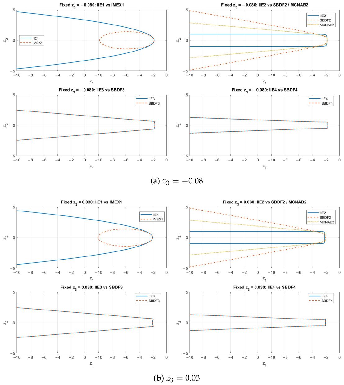
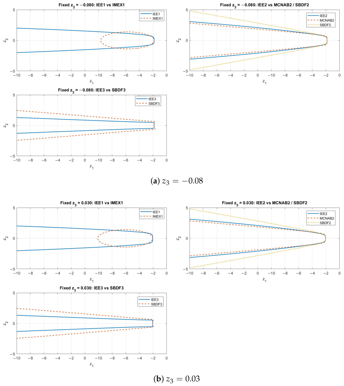
Our analysis indicates that variations in the reaction parameter $z_3$ within the interval $[-0.8,0.03]$ do not significantly alter the stability regions. This behavior is consistent with the relatively small magnitude of $z_3$ in the combustion model and indicates that the stability properties are dominated by the diffusion and advection contributions. Therefore, we present the graph of stability regions for $z_3=-0.08$ and $z_3=0.03$.

Figure 1 and Figure 2 show the contours of the stability regions for the additive splitting methods. In these plots, the stability region is bounded by the contours and the negative real axis. It can be observed that the first-order three-additive LMMs (IIE1 and IEE1) consistently yield larger stability regions than their IMEX counterparts, demonstrating enhanced robustness at low order. In contrast, the second-order three-additive LMMs exhibit noticeable deviations from the corresponding IMEX schemes (MCNAB2 and SBDF2). These differences arise because the second-order methods employ different multistep coefficients than their corresponding IMEX counterparts. By contrast, the third- and fourth-order methods share the same BDF-based implicit discretization as SBDF3 and SBDF4, resulting in largely comparable stability regions. Consequently, the influence of the additive splitting is more pronounced at second order than at higher orders. Furthermore, the relatively small magnitude of the reaction parameter $z_3$ means that it does not significantly alter the stability boundaries, which remain dominated by the diffusion and advection contributions.

5. Numerical Experiments

In this section, we compare the performance of the three-additive splitting methods (IIE and IEE) and the IMEX LMMs listed in Section 2 for the combustion model (5), with the temporal and spatial domains defined as $t\in [0,1]$ and $x\in [10,50]$, using $N=500$ grid points. All the simulations are run in MATLAB R2024b. Starting values and reference MOL solutions are computed with ode15s (AbsTol ${10}^{-12}$, RelTol $2.5\times {10}^{-12}$). As a validation of the reference solution, we recomputed the reference using MATLAB’s ode23tb solver with the same tolerance settings. Across all tested configurations (FKPP, Ignition, and Fisher reaction kinetics with $U_0\in \{0,0.75,0.99\}$), the final-time solutions obtained by ode15s and ode23tb agreed to within $\mathcal{O}\left({10}^{-10}\right)$ in the infinity norm, discrete $L^2$ norm, and relative norm. Therefore, the ode15s solution was used as the reference solution in the reported work–precision diagrams.

The implicit systems arising at each time step were solved using a modified Newton iteration. The most recent available numerical solution was used as the initial guess. At Newton iteration q, the nonlinear residual was written as

$$G\left(u^{\left(q\right)}\right)=u^{\left(q\right)}-\Delta t\left(b_{-1}^{\left[1\right]}{f}^{\left[1\right]}(t_{n+1},u^{\left(q\right)})+b_{-1}^{\left[2\right]}{f}^{\left[2\right]}(t_{n+1},u^{\left(q\right)})\right)-R_n,$$

where $R_n$ contains all known contributions from previous time levels and explicit terms. The Newton correction $\delta u^{\left(q\right)}$ was obtained from

$$J_G\left(u^{\left(q\right)}\right)\delta u^{\left(q\right)}=-G\left(u^{\left(q\right)}\right),$$

where

$$J_G\left(u^{\left(q\right)}\right)=I-\Delta t\left(b_{-1}^{\left[1\right]}{J}^{\left[1\right]}+b_{-1}^{\left[2\right]}{J}^{\left[2\right]}(u^{\left(q\right)})\right).$$

The sparse linear systems were solved using MATLAB’s backslash operator, which applies a sparse direct LU factorization. The Newton iteration was terminated when

$${\parallel \delta u^{\left(q\right)}\parallel }_2<{10}^{-15}$$

or when the maximum number of 20 iterations was reached. The same nonlinear tolerance, maximum iteration count, Jacobian construction, initial guess, and sparse linear solver were used for all methods to ensure a consistent comparison of CPU time.

To minimize random fluctuations, each test was repeated three times, and the smallest runtime was reported as a representative measure of computational performance. Each run used a constant stepsize $\Delta t={\displaystyle \frac{2^{-J}}{10}},J=0,1,\dots ,4$. Work–precision diagrams were used to compare the methods by plotting numerical accuracy versus CPU time. The numerical accuracy was quantified by using RMS error between the computed and reference solutions at the final time, defined as

$$\mathrm{RMS}=\sqrt{{\displaystyle \frac{1}{N}}\sum _{i=1}^N{\left(y_i^{\mathrm{num}}-y_i^{\mathrm{ref}}\right)}^2},$$

where $y_i^{\mathrm{num}}$ denotes the numerical solution, $y_i^{\mathrm{ref}}$ is the reference solution, and N is the number of spatial grid points.

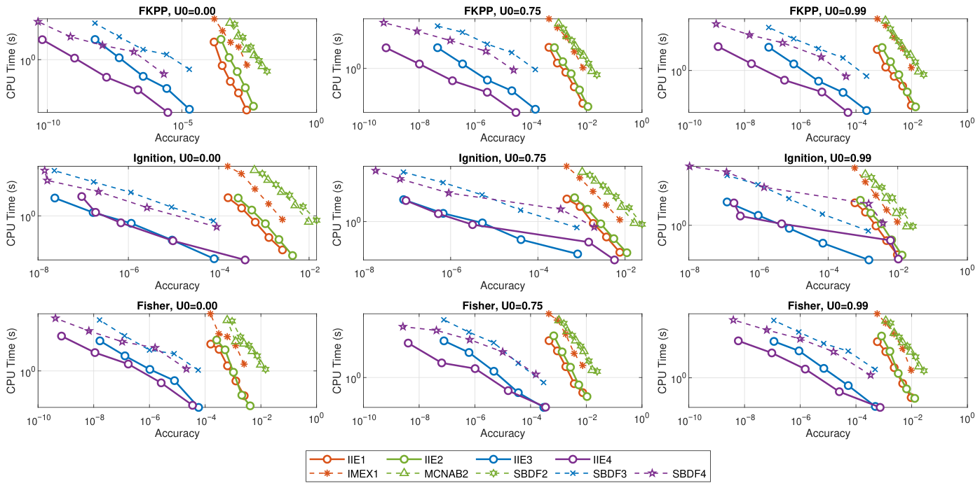
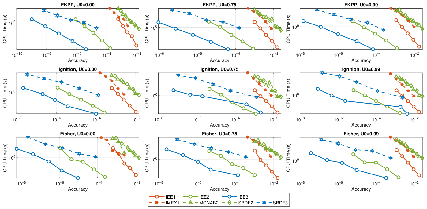
The work–precision diagrams of the experiments are shown in Figure 3 and Figure 4, and they demonstrate that the IIE and IEE methods achieve comparable or higher accuracy while requiring substantially less CPU time than the tested IMEX schemes across all experiments. Among these, the IIE3, IIE4, and IEE3 variants demonstrate the best overall efficiency, providing an optimal balance between the accuracy and computational cost for the combustion model under consideration. To provide a more detailed quantitative comparison, we have included all numerical results used to generate the work–precision diagrams in Appendix A. For each experiment, the appendix reports the RMS error, CPU time, and the speed-up factor, defined as CPU_IMEX/CPU_3-additive. A speed-up factor greater than one indicates that the three-additive method is computationally more efficient than its corresponding IMEX method, whereas a value less than one indicates that the IMEX method is faster. The appendix confirms the trends observed in the work–precision diagrams by showing that the three-additive methods achieve higher computational efficiency than their corresponding IMEX methods in nearly all experiments. Among all reported test cases, only a single experiment yielded a speed-up factor less than one, indicating that the IMEX method was faster in that particular case.

6. Conclusions

This work presented a systematic numerical assessment of three-additive linear multistep methods (IIE/IEE) for a stiff one-dimensional combustion model with FKPP, Ignition, and Fisher reaction kinetics, and compared their performance with widely used IMEX-LMM schemes. The numerical experiments demonstrated that the three-additive methods consistently achieve higher computational efficiency than the corresponding IMEX methods while maintaining comparable numerical accuracy across all tested configurations. These improvements arise from treating diffusion, reaction, and advection as separate components, allowing each process to be integrated using a numerical strategy appropriate to its characteristics.

The stability analysis complements the numerical experiments by showing that the first-order three-additive methods possess larger stability regions than their IMEX counterparts, whereas the higher-order methods retain largely comparable stability properties. Together, these results demonstrate that the additional flexibility provided by three-additive splitting can be achieved without compromising stability, making these methods an attractive alternative for stiff diffusion–reaction–advection systems.

The present study complements the theoretical analysis of the previously developed three-additive LMMs by demonstrating their practical effectiveness on a representative combustion model. Although the formulation requires separating the right-hand side into three components, this introduces little additional implementation complexity once the diffusion, reaction, and advection operators are available separately. The current investigation is limited to a one-dimensional combustion model. Future work will consider multidimensional DRA problems, strongly nonlinear systems, variable diffusion coefficients, and adaptive time-stepping strategies to further assess the applicability of the proposed framework to more realistic combustion simulations.

References

1. Ascher, U.M.; Ruuth, S.J.; Spiteri, R.J. Implicit-explicit Runge–Kutta methods for time-dependent partial differential equations. Appl. Numer. Math. 1997, 25, 151–167. [Google Scholar] [CrossRef] [Scilit]
2. Ruuth, S.J. Implicit-explicit methods for reaction-diffusion problems in pattern formation. J. Math. Biol. 1995, 34, 148–176. [Google Scholar] [CrossRef] [Scilit]
3. Hundsdorfer, W.; Verwer, J.G. Numerical Solution of Time-Dependent Advection-Diffusion-Reaction Equations; Springer: Berlin/Heidelberg, Germany, 2003. [Google Scholar] [CrossRef] [Scilit]
4. Dimarco, G.; Pareschi, L. Implicit-Explicit Linear Multistep Methods for Stiff Kinetic Equations. SIAM J. Numer. Anal. 2016, 55, 667–690. [Google Scholar] [CrossRef] [Scilit]
5. Griepentrog, E. Gemischte Runge-Kutta-verfahren fur steife systeme. Semin. Sekt. Math. 1978, 11, 19–29. [Google Scholar]
6. Hofer, E. A Partially Implicit Method for Large Stiff Systems of ODE’s with Only Few Equations Introducing Small Time-Constants. SIAM J. Numer. Anal. 1976, 13, 645–663. [Google Scholar] [CrossRef] [Scilit]
7. Crouzeix, M. Une méthode multipas implicite-explicite pour l’approximation des équations d’évolution paraboliques. Numer. Math. 1980, 35, 257–276. [Google Scholar] [CrossRef] [Scilit]
8. Boscarino, S.; Pareschi, L.; Russo, G. Implicit–Explicit Runge–Kutta Schemes for Hyperbolic Systems and Kinetic Equations in the Diffusion Limit. Symmetry 2018, 10, 148. [Google Scholar] [CrossRef] [Scilit]
9. Hundsdorfer, W.; Ruuth, S.J. IMEX extensions of linear multistep methods with general monotonicity and boundedness properties. J. Comput. Phys. 2007, 225, 2016–2042. [Google Scholar] [CrossRef] [Scilit]
10. Hundsdorfer, W. Stability Analysis of Time Integration Methods for Stiff Differential Equations. Symmetry 2020, 12, 1023. [Google Scholar] [CrossRef] [Scilit]
11. Mara’Beh, R.A.; Spiteri, R.J.; González, P.; Mantas, J.M. 3-additive linear multi-step methods for diffusion-reaction-advection models. Appl. Numer. Math. 2023, 183, 15–38. [Google Scholar] [CrossRef] [Scilit]
12. Bianco, F.; Chibbaro, S.; Prud, R. Etude d’une Equation de Convection-Reaction-Diffusion en Ecoulement Compressible. 2011. Available online: http://nonlineaire.univ-lille.fr/SNL/media/2011/resumes/CHIBBARO_sergio.pdf (accessed on 4 July 2026).
13. Echekki, T.; Mastorakos, E. Fluid Mechanics and Its Applications. In Turbulent Combustion Modeling; Springer: Dordrecht, The Netherlands, 2011; Volume 95. [Google Scholar]
14. Preuss, A.; Lipoth, J.; Spiteri, R.J. When and how to split? A comparison of two IMEX splitting techniques for solving advection–diffusion–reaction equations. J. Comput. Appl. Math. 2022, 414, 114418. [Google Scholar] [CrossRef] [Scilit]
15. Mara’Beh, R.A.; Mantas, J.; González, P.; Spiteri, R.J. Performance comparison of variable-stepsize IMEX SBDF methods on advection-diffusion-reaction models. Comput. Math. Appl. 2025, 190, 41–56. [Google Scholar] [CrossRef] [Scilit]
Figure 1. Comparison of stability regions for IIE and IMEX methods.
Mathematics 14 02475 g001
Figure 2. Comparison of stability regions for IEE and IMEX methods.
Mathematics 14 02475 g002
Figure 3. Work–precision plots for the IIE and IMEX methods.
Mathematics 14 02475 g003
Figure 4. Work–precision plots for IEE and IMEX methods.
Mathematics 14 02475 g004