


Abstract
Forecasting foreign exchange rates over long time periods depends on economic fundamentals. Short-term predictions, by contrast, depend largely on emotions, governmental announcements, the flow of capital, and media commentary. This paper proposes a suite of methods, collectively referred to as ForExAI, to predict foreign exchange rates based on time series analysis and news article analysis. The time series analysis is based on classical statistical time series techniques, such as ARIMA, as well as machine learning methods using neural networks. Separately, ForExAI uses Large Language Models to analyze news articles based on two kinds of prompts: (i) expert-written based on econometric considerations, (ii) existing prompts documented in the literature. Our findings on time series of exchange rates indicate that there are signals in the time series that can be captured even by simple methods like ARIMA(1,1,1), as well as novel machine learning methods on the time series of foreign exchange rate trades. Further, an adaptation of the Kelly criterion can increase cumulative profits. Finally, an ensemble approach often delivers slightly lower profit, but also lower volatility, leading to a higher Sharpe ratio. Regarding news article analysis, shorter prompts yield far better results than complex ones derived from expert knowledge. This work shows a method for hyperparameter tuning a collection of models that forecast complex time series, as well as the relative virtues of different versions of the Kelly criterion. The results make a pragmatic contribution as well. Because we measure profits ignoring transaction costs, our work is not directly actionable by traders, but the insights could be useful. In addition, our results point to further areas of research for traders.
Keywords:
high-frequency trading; foreign exchange; forecasting; transformers; N-BEATS; N-HiTS; ARIMA; large language models; expert prompts; zero-shot learning; event-driven algorithmic trading MSC:
68-04
JEL Classification:
C45; C53; C63; G12
1. Introduction
Foreign exchange (FX) markets move more than 7.5 trillion United States Dollars (USD) each day, making them the most liquid but also one of the most volatile financial domains in the world [1]. Price dynamics are driven not only by their own autocorrelated technical patterns but also by exogenous macroeconomic events that are reported through global news outlets.
Statistical forecasting methods such as ARIMA [2] and neural networks capture autoregressive patterns yet ignore the semantic signals embedded in breaking headlines. In contrast, natural language processing (NLP) models that infer sentiment from news or social media often react after large moves have already materialized, so it is a struggle to convert their sentiment to profitable trades.
Motivated by these complementary shortcomings, we present ForExAI, a suite of forecasting frameworks that models both univariate time series inference and real-time news article analysis to predict the direction of profitable trades.
We study the currency pairs USD/BRL (US dollar vs. Brazilian Real), USD/CNY (US dollar vs. Chinese Yuan), USD/Euro, and USD/GBP (US dollar vs. British pound) markets over a testing period of 11 months for USD/CNY and USD/BRL, and 16 months for USD/EUR and USD/GBP. Note that the Brazilian Real, Euro, and British Pound trade freely in foreign exchange markets, whereas the Yuan is quite regulated [3]. Our results show that ForExAI delivers statistically significant gains in total profit and profit-per-trade, for the uncontrolled exchange rates, assuming no transaction costs. It also shows gains for the USD/CNY, but those are modest. Such results can be the basis both for further investigation for traders and for market makers. While market makers do not have to pay transaction costs (and sometimes profit from them), they do incur inventory risk. Thus, while our work does not immediately lead to a method for making profits, our methods show signals in foreign exchange markets.
Contributions of ForExAI
This work makes the following contributions:
- Empirical Time Series Forecasting: Studies the behavior and profitability of several high-capacity LLM-based time series models, several neural network-based forecasters for time series, classical forecasting techniques, and simple techniques such as mean reversion, trend, and crossover techniques.
- Empirical News-Related: For news articles, we test several Large Language Models for news sentiment.
- System: Unifies these approaches through an ensemble model that explicitly learns each model’s contribution.
- Theoretical: Assesses the performance of taking positions based on two principled variants of the Kelly criterion as well as fixed positions. Relating predictions of gains and history of gains to the Kelly criterion’s notion of pay-off constitutes the main conceptual (as opposed to empirical) contribution of this paper.
This paper describes the design choices made in the construction of ForExAI and experimentally documents the impact of these choices on trading performance.
2. Base Time Series Methods
This section describes the forecasting and classification methods used to generate predictive signals for the trading strategies detailed in Section 5.2, based solely on time series data (i.e., without looking at news) consisting of sequences of exchange rates. We use several time series forecasting models that learn the next-step mid-price from some subsequence of prices up to the current time: classical econometric approaches such as ARIMA, (ii) neural network architectures (N-BEATS, N-HiTS, and TCN); and (iii) large pre-trained foundation models (Chronos–Bolt and Toto) applied in a zero-shot forecasting setting without task-specific fine-tuning. The predicted mid-prices from these models serve as the basis for the model-driven trading strategies (Section 5.2), which use the direction of the predicted price movement to determine whether to buy, sell, or hold a currency position.
2.1. Classical Forecasting Models
Traditional econometric models such as ARIMA and GARCH have served as foundational tools for modeling the autocorrelated structure of financial time series [2]. These models excel at capturing linear dependencies and volatility clustering, respectively, but struggle to generalize in the presence of non-stationarity or regime shifts. When embedded in trading strategies, forecasts from an ARIMA(1,1,1) specification typically do not generate profits that are statistically different from random trading, reflecting the near-martingale behavior of financial results.
The Autoregressive Fractionally Integrated Moving Average (ARFIMA) model [4,5,6] is an extension of the standard ARIMA class of models, specifically designed to capture long memory and persistence in time series data. While traditional ARMA models are suited for short-memory processes where the influence of past shocks decays exponentially, and ARIMA models handle non-stationarity through integer differencing, many series in finance and economics exhibit a persistence that is stronger than an ARMA process but is still mean-reverting, unlike a unit-root process.
In ARFIMA models with , convergence to the unconditional mean occurs slowly due to long memory. Therefore, although ARFIMA forecasts may display greater persistence at short and medium horizons, dynamic multi-step predictions eventually become flat, similarly to dynamic ARIMA models. This behavior is a direct consequence of the long-memory structure described in [4,5,7] rather than a limitation of estimation or model specification. For these reasons, we use a static ARIMA model only.
2.2. Neural Network-Based Forecasting Models
We consider two categories of neural network-based forecasting models: (i) models that are trained on the training dataset of the time series dataset, and (ii) large pre-trained foundation models applied in a zero-shot setting without task-specific retraining (though with hyperparameter selection).
2.2.1. Models Requiring Training
The models requiring training include N-BEATS, N-HiTS, and the Temporal Convolution Network (TCN). Our experimental methodology replicates our previous work [8], but we briefly summarize it here for completeness.
N-BEATS: N-BEATS [9] is a deep feedforward forecasting model built from a sequence of residual blocks that iteratively refine predictions. Each block produces two outputs: a “backcast,” which reconstructs the input window, and a “forecast,” which contributes to the final prediction [9]. This residual design helps isolate trend and seasonal components, enabling the model to progressively capture unexplained patterns while maintaining interpretability and strong predictive accuracy [9]. Our implementation uses one block and two stacks, each block consisting of five fully connected layers of width 512 with dropout (0.2).
N-HiTS: N-HiTS [10] extends N-BEATS by introducing a hierarchical structure that models temporal patterns at multiple resolutions. By analyzing the time series at coarse and fine scales, the model captures both short-term fluctuations and longer-term dynamics [10]. It also incorporates interpolation layers to enhance robustness and smoothness in the forecasts [10]. Our implementation has one block and two stacks of five layers each, using feed-forward layers of width 512 and dropout 0.2.
Temporal Convolution Network (TCN): TCNs [11,12,13] apply one-dimensional convolutions in a causal and dilated fashion, ensuring that each prediction depends only on past inputs while efficiently covering long time horizons. Residual and skip connections stabilize deep architectures, allowing the model to learn complex temporal dependencies without gradient degradation [11,12,13]. Our implementation uses eight convolutional layers with 64 filters and a kernel size of 3. A dilation base of 2 and weight normalization are applied, with dropout 0.2 for regularization.
2.3. Zero-Shot Models
In contrast to the trained models, Chronos–Bolt and Toto are applied in a zero-shot forecasting setting. These models are large-scale, pre-trained time series foundation models, and we evaluate their out-of-the-box generalization to our data without fine-tuning.
2.3.1. Chronos–Bolt
As described in detail in the related work section Section 20.2, Chronos–Bolt [14] represents an evolution over the original Chronos framework (the Chronos authors request that the same paper reference be used for both Chronos and Chronos–Bolt) and serves as our initial benchmark in this category. In our experiments, we have used the 204M parameter Transformer-based model.
We ingest raw mid-price sequences, delegating the handling of non-stationarity to the model’s intrinsic Instance Normalization layer. Given a historical context window C, the length of which is optimized via hyperparameter search in Section 10, the input is standardized using its local moments. Consequently, the model operates within a normalized space defined by: , where and represent, respectively, the mean and standard deviation of the input window (which is the time period and data that Chronos–Bolt looks at to make a prediction). This adaptive standardization enables the handling of local volatility without need for external scaling.
Chronos–Bolt generates probabilistic forecasts via a regression-based head, targeting a specific set of quantile levels defined during training . This allows predictions to extend beyond the observed input range when supported by the underlying trend. For our trading signal, we isolate the median forecast ( quantile) as the deterministic prediction, . To recover the final price estimate, the inverse affine transformation is applied using the context statistics: . Recall that and are derived exclusively from the input window and thus can change as the time series evolves.
2.3.2. Toto Foundation Model for Financial Time Series Forecasting
Toto [15] is a large-scale 115M parameter foundation model for time-series forecasting that, like Chronos–Bolt [14], operates in a zero-shot setting. Toto is designed to generalize across diverse temporal domains without any task-specific fine-tuning. As such, it employs an internal instance normalization strategy similar to that of Chronos–Bolt to handle distributional shifts. Consequently, we provide raw mid-price sequences to the model, relying on its internal mechanism to standardize inputs based on the local context statistics. This approach ensures that the model adapts to the specific volatility of the input window without requiring training set access.
During inference, Toto generates multiple probabilistic samples for each forecast point. In our experiments, we set the sampling parameter to 64 time steps. We then used the median prediction across samples as the final point forecast. We set the time interval to 60 s to reflect the one-minute spacing in our forex data.
3. Event-Based News-Reading Forecasting Methods
The news analysis portion of our work poses the following question: to what extent do news articles anticipate foreign exchange rate movements? We looked to Large Language Model prompts to convert such news articles into trading signals for two very different exchange scenarios: USD/Chinese Yuan and USD/Brazilian Real.
3.1. News Article Classification Prompts for the Chinese Yuan vs. U.S. Dollar
There are three news prediction prompts for the Chinese Yuan (CNY) vs. U.S. Dollar (USD): a Naive prompt, a Naive+ prompt, and an Expert prompt. All prompts ask the LLM to classify a news article into three categories:
- : Expected CNY appreciation (exchange rate of CNY against USD increase)
- : Expected CNY depreciation (exchange rate of CNY against USD decrease)
- : Neutral sentiment or conflicting signals
The Naive prompt specifies the minimal prompt to predict an article’s impact on an exchange rate. This prompt serves as a baseline.

3.1.1. Naive+ Prompt
The Naive+ prompt extends the Naive prompt with a reference to the relevant currency. This prompt allows for comparing and contrasting with the performance of the Naive prompt. Informally, we hypothesize that additional detail in the prompt will improve performance.

3.1.2. Expert Prompt
The Expert prompt (Appendix B.1) is derived from discussions with one of the co-authors (E.H.), who is an economist. The prompt is designed to operationalize analyst-like behavior. The prompt is tailored specifically to the CNY/USD currency pair, targeting foreign-exchange analysis in offshore Chinese yuan and U.S. dollars. The Expert prompt includes illustrative examples, which are used to shape outputs and to enforce consistent labeling behavior across tasks.
Note that all prompts are used as a “zero-shot” (or “few-shot” in the case of examples) classification. They do not embed domain knowledge.
The prompts (Naive, Naive+, Expert) are used to predict the influence of single news articles on exchange rates. In Section 11, we use training data to tune the hold period hyperparameter (in minutes) for fixed-position size trading. Based on this analysis, we select the best-performing news event model for the USD/CNY exchange rate and test this model/hold period combination on the test data.
3.2. News Article Classification for the Brazilian Real vs. U.S. Dollar
Focusing on the Brazilian Real (BRL)/United States Dollar (USD) exchange rate, we formulate sentiment classification as a three-class problem predicting exchange rate movement direction (up, down, or neutral) given news articles. We assess performance through profitability analysis, comparing trading strategies based on model predictions against market benchmarks.
Given a news article, we use an LLM that infers the expected direction of BRL movement. We formulate this as a three-class classification problem:
where the predicted classes correspond to expected BRL/USD exchange rate movements:
- Up: Expected BRL appreciation (USD/BRL rate decreases)
- Down: Expected BRL depreciation (USD/BRL rate increases)
- Neutral: No significant movement or conflicting signals
3.2.1. Inference Pipeline
We adopted a pipeline utilizing meta-llama/Llama-3.1-70B-Instruct with a temperature of 0 and lucas-leme/FinBERT-PT-BR. The Llama 3.1 70B model provides strong reasoning capabilities and output consistency without the extreme latency of the 405B model, while FinBERT-PT-BR provided a robust, domain-specific baseline for Brazilian Portuguese financial text.
3.2.2. Prompt Engineering Methodology
We design a systematic prompt engineering strategy developed in collaboration with a financial expert (co-author E.H.), progressing through three distinct approaches with increasing levels of task specification and domain knowledge:
Basic Zero-Shot (P0):
Simple prompts establishing the basic role and task.
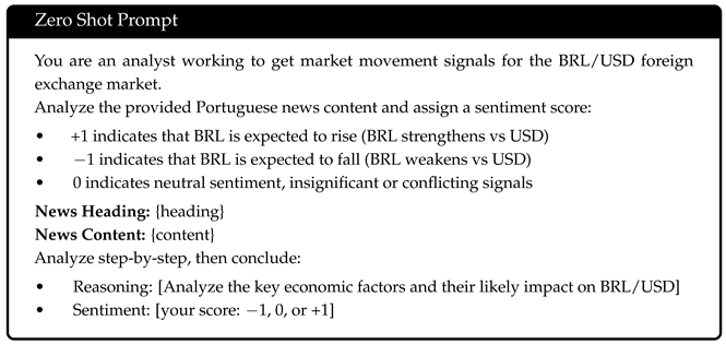
Expert-Guided Zero-Shot (P1):
We used domain expert insights to extend P0 to build a more comprehensive prompt (Appendix B.2) that defines the classification task by refining the prompt with financial criteria. These criteria include market drivers such as US Federal Reserve policy, Brazilian fiscal measures, trade balance, and commodity factors, with specific rules for each variable.
Expert Framework with Examples (P2):
The expert-guided prompt enhanced with few-shot learning using curated examples per class selected to demonstrate the application of the actionable insights across diverse market scenarios, including fiscal policy changes, monetary policy shifts, and commodity price movements. After initial experimentation on the training data with 1, 3, and 5 examples per class, we selected 1 example per class as it best balanced performance with minimal computational overhead (Appendix B.3).
Similar to our proposed USD/CNY prompts, in Section 11.5, we use training data to tune the hold period hyperparameter (in minutes) for fixed-position size trading. Based on this analysis, we select the best-performing news-event model for the USD/BRL exchange rate.
3.3. Comparative News-Event Model Baselines
To establish a comparative baseline for news-event trading, we adopt the prompt engineering framework proposed by Fatouros et al. [16], originally evaluated on FinBERT and GPT-3.5. For our experiments, we employ Llama 3.1 8B Instruct [17] as the generative backbone. While Fatouros et al. utilized six distinct prompts, we restrict our evaluation to the four instance-level (an instance is a single headline) prompts listed below. We exclude the remaining two prompts, which group all the headlines of a given day, because we wanted to compare the approaches on single articles. (In [16], the authors report that no single prompt performed best everywhere, so this exclusion doesn’t eliminate their best-performing approach.) During inference, we utilize a temperature setting of 0, dynamically substituting the template variables (prefixed with $) with the corresponding ticker symbol and headline text. In instances where the model output deviates from the expected token vocabulary, the sample is assigned a ’neutral’ label. To ensure a fair comparison against our proposed prompts, these baseline prompts were executed using an identical inference pipeline, ensuring that any variation in profitability stems directly from the prompt structure rather than backend generation differences.


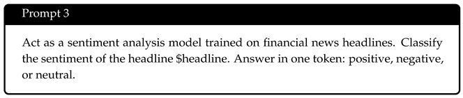
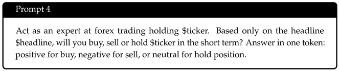
A second sentiment analysis approach is the prompt engineering framework proposed by Ballinari and Maly [18] (Appendix B.4). Their study provides a comparative analysis spanning rule-based lexical systems (Loughran-McDonald, VADER), domain-specific encoders (FinBERT), and the generative Llama 3.1 8B Instruct model, evaluating the latter in both zero-shot and task-specific fine-tuned configurations. For our experiments, we utilize the Llama 3.1 8B Instruct model with its official off-the-shelf weights. Following default settings, inference is conducted at a temperature of 0.6. We dynamically populate the template placeholders (denoted by $) with the specific ticker, title and body text of each news entry to generate directional labels for the target currency.
Note that, following the usage of comparative models in the literature, the trading strategy for these models is “hold until the close of the day.” In contrast, for our prompts in Section 11.5, we treat the hold period as a hyperparameter and tune it for each prompt.
4. Datasets
We use three dataset types: foreign exchange price data, financial news articles (for Chinese Yuan/USD and Brazilian Real/USD), and a collection of news articles, a subset of which are labeled by an expert. Prices reflect short-term market dynamics (within a few minutes), while news may take longer to have an effect, and its effect may last longer.
4.1. FX Price Data
The foreign exchange price data for USD/CNY (U.S. dollar vs. Chinese Yuan) and USD/BRL (U.S. dollar vs. Brazilian Real) were obtained from https://massive.com [19], which provides historical and real-time financial market data. For USD/EUR (U.S. dollar vs. Euro) and USD/GBP (U.S. dollar vs. British Pound), the data were obtained from Bloomberg [20].
Both the bid (buy) and ask (sell) prices were collected at each trade to compute the mid-price, as defined in Equation (2). The resulting mid-price series serves as the primary signal for both model training and inference during trading simulations. The data were collected at a resolution of at most one minute.
The overall sample covers the period from 1 January 2024 to 31 July 2025 for USD/CNY and USD/BRL and 1 January 2024 to 31 December 2025 for USD/EUR and USD/GBP. Specifically, the training dataset spans 1 January–30 June 2024 for all currencies (used to train the models described in Section 2.2.1); the validation dataset spans 1 July–31 August 2024 for all currencies (used to select, for each model described in Section 2.2, the optimal input context length and Kelly parameters, namely the rolling window size d, warm-up length N, and initial fixed fraction defined in Section 6, via grid search on the validation profit, as detailed in Section 10); and the test dataset spans 1 September 2024–31 July 2025 for USD/CNY and USD/BRL and 1 September 2024–31 December 2025 for USD/EUR and USD/GBP (used to evaluate the selected configurations under the trading strategies described in Section 5, with out-of-sample results reported in Section 13 for all currency pairs). For testing, trading was simulated between 9 a.m. and 5 p.m. U.S. Eastern time, when the markets are most active.
To characterize the price dynamics of each currency pair, we report the annualized volatility of the mid-price series, computed from logarithmic returns. Specifically, for a series of mid-prices , the logarithmic return at each period is , and the annualized volatility is , where is the sample standard deviation of computed over the full dataset. The resulting annualized volatilities are reported in Table 1.
Table 1.
Annualized volatility of the mid-price series for each currency pair, computed from logarithmic returns over the full dataset.
The volatility estimates are consistent with the known regulatory regimes of each currency. USD/BRL exhibits the highest annualized volatility (0.0120), reflecting the fact that the Brazilian Real trades freely in open foreign exchange markets and is therefore subject to the full influence of macroeconomic events, capital flows, and investor sentiment. USD/EUR (0.0028) and USD/GBP (0.0026) show moderate and closely comparable volatility levels, as both currencies are freely floating and deeply liquid. USD/CNY, by contrast, exhibits by far the lowest annualized volatility (0.0015), roughly half that of USD/EUR and USD/GBP, and an eighth that of USD/BRL. We will see that this has consequences in our forecasting.
4.2. News Articles
Brazilian Real News Articles: The articles used in our experiments span the period from 12 January 2024 to 30 July 2025, comprising a total of 25,226 articles. These articles were scraped, cleaned, and aggregated from Bom Dia Mercado (Good Morning Market, https://www.bomdiamercado.com.br, accessed on 7 September 2025), a Brazilian financial news wire service. The dataset contains articles with corresponding timestamps at minute-level granularity. The dataset was divided as follows: a subset of articles from 12 January 2024 through 30 June 2024 were used for training and parameter tuning, and the articles from 1 September 2024 through 30 July 2025 were used for testing. Note that in the case of an update to an existing news article, a new version of the article (with a new timestamp) is published.
Chinese Yuan News Articles: The news articles for our experiment were collected between 19 January 2024, and 30 July 2025. In total, 2685 news articles for the currency pair U.S. Dollar and Yuan were obtained over this period, with timestamps recorded at the minute level. We divide the dataset into a training set containing 827 articles from 19 January to 30 June 2024, and a test set containing 1858 articles from 1st September 2024, to 30 July 2025. The news articles themselves were drawn from the LSE Thomson Reuters newswire service [21]. Note that in the case of an update to an existing news article, a new version of the article (with a new timestamp) is published.
5. Time Series-Based Trading Strategies
Time series-based trading strategies look only at the time series of exchange rates, not at news articles or other quantitative indicators. These strategies act on the mid-price, defined as the average of the bid and ask quotes:
where denotes the mid-price of the USD/CNY, USD/BRL, USD/GBP, or USD/EUR exchange rate at time t, is the ask price at time t, and is the bid price at time t. Here, Currency A is the base currency (USD) and Currency B is the quote currency (CNY, BRL, GBP, or EUR). A “buy” action corresponds to going long on USD (buying Currency A, selling Currency B), while a “sell” action corresponds to going short on USD (selling Currency A, buying Currency B). The holding time is one minute. In an environment with transaction costs, holding times may be extended if the current position (e.g., long on currency X and short on currency Y) is still suggested by the model at the end of the holding period.
At each time step t, the fractional change in mid-price is computed as:
The trading rules described throughout this section use a threshold parameter to determine whether a predicted movement is sufficiently large to trigger a trade. Additional experiments using positive threshold values () are described in Appendix A.1.
5.1. Rule-Based Strategies
The strategies Mean Reversion, Trend, and Moving Average Crossover operate purely on previously observed changes in exchange rates. They rely on rule-based heuristics that predict that exchange rate changes will reverse or that they will continue.
5.1.1. Mean Reversion Strategy
The mean reversion strategy assumes that deviations from recent trends are temporary and prices will revert to their previous states. The trading decision is defined as:
5.1.2. Trend Strategy
The trend-following strategy assumes that price movements will persist in the same direction. The decision rule is the opposite of mean reversion:
5.1.3. Moving Average Crossover Strategy
The moving average crossover strategy detects persistent trend reversals by identifying the moment at which two smoothed versions of the price series, computed over different time horizons, switch relative positions [22]. A simple moving average (SMA) of length k is defined as:
where k is the window length and corresponds to lagged mid-prices. Let s denote the short window and l the long window, with . A signal is generated only at the moment the two averages cross. The trading decision is defined as:
Any open position is closed either when the two moving averages converge to equality, , or when an opposite crossover signal arrives. In empirical finance applications, common parameter choices include trading days [22,23]. The optimal pair for each currency pair is selected on the validation dataset using the procedure described in Section 10.
5.2. Model-Driven Strategies
The second group of strategies consists of machine learning models as described in Section 2.2, either directly or as part of an ensemble system. These models infer the next mid-price based on historical context.
Formally, given the past n timesteps, a model forecasts the mid-price at :
where corresponds to machine learning (ML) models and large language models (LLMs) adapted for time series forecasting, detailed in Section 2.2, and n represents the input context length of the model.
The predicted percentage change is:
The trading rule is as follows:
Beyond trading profitability, we assess the raw predictive accuracy of each forecasting model f by comparing the predicted fractional price change (Equation (9)) against the realized change (Equation (3)) on the test data. Predictive accuracy is measured using four metrics: root mean squared error (RMSE), mean absolute scaled error (MASE), mean absolute percentage error (MAPE), and symmetric mean absolute percentage error (sMAPE). The results are reported in Section 17.
5.3. Ensemble Strategy
The ensemble strategy consolidates the predictive signals produced by the previously described strategies, using a regression model to infer the next price movement directly from the real-valued percentage changes predicted by each strategy.
At each time step t, let denote the predicted percentage change generated by the mean reversion strategy. The trend strategy is not included, as its predicted price change is exactly the negative of mean reversion and would therefore add no new information. Let denote the predicted percentage change produced by the i-th forecasting model, where and the forecasting models are described in Section 2.2.
The ensemble feature vector at time t is constructed by concatenating these real-valued predictions:
A regression function , implemented as a Ridge Linear Regressor, is trained to map this feature vector to a predicted percentage change in mid-price from one timestep to the next:
The model is trained using historical data, where the supervision signal is the realized mid-price change:
computed using mid-prices outside market hours to avoid lookahead bias.
In our implementation, the regression model g is retrained in a rolling manner to reflect the most recent market dynamics. Specifically, on each trading day d, the regressor used for inference is trained exclusively on data observed prior to day d, ensuring that no future information is incorporated. This training procedure is executed once per day at 9:00 a.m., immediately before the start of the trading window. To determine the optimal regularization parameter of the Ridge regressor, we employ hyperparameter optimization via Optuna [24], using a time series cross-validation scheme. is selected by trying values between and 100. For each candidate value, the model is trained and evaluated three times on consecutive, non-overlapping windows of the most recent 80% of available historical data, always training on earlier data and testing on later data to respect the time ordering. The candidate value that produces the lowest average prediction error across the three evaluations is selected. Based on experimentation on the validation data, re-optimizing the ridge regressor hyperparameter once per week produces the best results.
The resulting predicted change is then converted into a trading action:
Since is linear, the fitted coefficient associated with the i-th component of directly quantifies the contribution of model i to the ensemble forecast. These weights are interpretable: a positive means the ensemble has learned, from historical data, to trust model i’s predicted price movement, while a negative means the ensemble has learned to invert it, indicating that model i’s predictions are opposed to realized price movements. The magnitude of reflects the relative influence of each component, providing a data-driven ranking of forecaster usefulness for each currency pair.
6. Time Series-Based Trading: Kelly-Based Position Sizing
The Kelly fraction is computed dynamically to adjust position sizes based on the observed performance of each trading strategy.
For each strategy (e.g., mean reversion, Chronos–Bolt), we maintain and update after every trade:
- , : counts of winning and losing trades,
- : sum of positive profits,
- : sum of absolute losses.
- Thus, , , , and all change after each new trade. In our implementation, these running statistics are computed over a rolling window of the most recent d trading days rather than over the full history. This windowing allows the estimates to adapt to non-stationary market conditions, giving greater weight to recent performance while discarding outdated information that may no longer be representative. The optimal window length d is determined using the validation dataset to maximize overall profitability, and the selected values for each strategy are reported in Section 10.
From these running statistics, after trade t, we estimate:
Here, is the empirical ratio of the average gain when a method wins with the average gain when the method loses. This ratio is thus analogous to the payoff in the original Kelly formulation when a bettor accepts b (average gain) to 1 (average loss) odds. While the calculation of looks at history, we also want to take into account the prediction for the next trade.
To incorporate the model’s prediction for the current trade, we also keep track of predicted gains. Let
be the running average of all predicted gains up to and including trade t (even for trades that ultimately lose). We then define a prediction-based weight
The Kelly fraction for trade t is then
Relationship to the Classical Kelly formula: Equation (23) has the same form as the classical Kelly formula, viz. , where p and q () are the win and lose probabilities and b is the payoff odds. Our p and q are the same as for Kelly. The term is an approximation of the payoff odds. Thus, the higher (the historic payoff) and the higher (the predicted gain relative to the historical gain), the greater the bet.
In practice, we separate the procedure into a short “warm-up” phase and a Kelly-driven phase. For the first N trades, we do not trust the early estimates of , , and (because there are too few wins and losses), so we use a fixed, small fraction ,
solely to accumulate enough data to stabilize , , , and . The hyperparameters N and are determined using the validation dataset, where they are selected to maximize overall profitability. The resulting values for each strategy are reported in Section 10.
After this warm-up period (), we switch to the model-weighted Kelly fraction (23) to size positions:
The Kelly formula can produce negative values when either the probability of losing is high or the win–loss ratio is unfavorable. In those cases, we set the Kelly fraction to 0 and trade nothing.
6.1. Active vs. Passive Kelly
We call a strategy that changes , , , and only when equation model actually trades Active Kelly. That is, only when Equation (25) is in the case do any of , , , or .
However, even when a method under Kelly trades nothing, it could still keep track of whether its predictions were correct or not. That would influence and . Thus, if a prediction were correct, that could increase even though no trade happens. However, for the purpose of the calculations of and , and are affected only by situations in which an actual trade based on the prediction takes place. We call a strategy that changes and , though not , and even when Kelly suggests a zero bet Passive Kelly.
Formally, we keep track of another two variables and that are updated every time a prediction is made, regardless of whether . In contrast, and are updated only when . The update rules then proceed as follows:
- , : counts of winning and losing trades,
- , : counts of winning and losing predictions
That is, the calculation for changes, which causes the calculation for to change, because those have to do with the probabilities of wins and losses but not their magnitudes. The magnitude calculations for and remain the same. Gathering win/loss information even when not trading intuitively should help. The experiments show otherwise, as we will see.
7. News Article-Time Trading: Position Size and Hold Period
Our LLM models for news analysis predict only the direction of a currency exchange rate change based on the content of the article. These predictions are converted into a fixed-sized and fixed-hold period trading strategy. We use a fixed-sized bet rather than a variable Kelly-based method because news article analysis predicts only a direction, not a predicted gain, so using the Kelly criterion is not appropriate. For time series predictions, our models predict exchange rate prices. These price predictions are converted into a variable-sized trading and a variable-hold strategy.
Fixed Position Size and Hold for News Analysis
In the fixed position scheme, each trade (long or short) is executed with a constant position size of
There are three other policy decisions with respect to fixed-sized and fixed-hold trading on news articles.
- 1.
- If multiple events occur during the same time period, a single trade is executed on the basis of the majority vote. If there is no majority, no trade is executed.
- 2.
- If an event occurs while an existing trade is executing, a new independent trade is executed. Thus, multiple trades may be executed simultaneously and may be in different directions.
- 3.
- At the end of the trading day (5 pm), all trades are closed, regardless of the remaining hold time. In other words, no trades are held beyond 5 pm.
8. Evaluation Metrics for the Experiments Based Purely on the Exchange Rate Time Series
For time series trading, to obtain stable and comparable estimates across strategies and currency pairs, each trading strategy was executed times using different random seeds, where each run () represents a complete trading simulation. This repetition helps account for stochastic variation due to model initialization and sampling effects in the models and configurations selected from Section 10, ensuring that the reported results reflect consistent, expectation-based performance rather than outcomes from a single random realization. We then aggregate the resulting outcomes.
For News article trading, with the temperature set to 0, we execute the trading simulation 10 times with different random seeds, since current LLM architectures have slight variations due to various system factors. The results did not vary significantly due to these system variations.
We report five evaluation metrics: the average cumulative profit (ACP), the average profit per trade (APPT), the annualized average monthly Sharpe ratio (AAMSR) computed by averaging the monthly Sharpe ratios, then annualizing by multiplying by , average maximum drawdown (AMDD), and average skewness (ASKEW). The ACP measures overall effectiveness of a model. The APPT measures effectiveness of a model on a basis relative to each trade, providing some evidence of how the model would interactive with trading costs. The sharpe ratio is a measure relative reward to risk (as measured by the standard deviation of returns). Maximum drawdown is another measure of risk. Finally, skewness measures the distribution of returns around the mean. Positive skew shapes tend toward profitability.
Let denote the profit of strategy s at time t in run . Because of randomness, some runs may bet at time t and others may not. Let the total number of trades over all runs (between 1 and J) and all times (between 1 and T) be . The average profit per trade (APPT) for strategy s for all runs and all times up to T is then:
The average cumulative profit () for method s is simply the total profit divided by J:
For the Annualized Average Monthly Sharpe ratio, profits are first aggregated at the monthly level. Let denote the set of time indices belonging to month m, and define the monthly profit for run j as
We then compute the average monthly profit across runs:
Let and denote the mean and standard deviation of across all months. In keeping with standard financial reporting [25], we report the Annualized Average Monthly Sharpe ratio as defined by:
Maximum drawdown measures the worst sustained loss experienced by a strategy over the evaluation horizon and is widely used as a practical measure of downside risk. It captures the largest decline from a previous portfolio peak to a subsequent trough. Let denote the cumulative portfolio value of strategy s at time t for run j. Define the peak portfolio value up to time t as:
The maximum drawdown for run j is then:
The average maximum drawdown across all runs is:
More negative drawdown values indicate larger sustained losses and therefore higher portfolio risk.
Finally, we report skewness as a measure of asymmetry in the distribution of profits. Positive skewness indicates that the distribution contains relatively larger positive outcomes compared to negative outcomes, whereas negative skewness indicates the opposite. Because trading profit distributions are often non-symmetric, skewness provides additional information beyond the mean and variance regarding the shape of the return distribution.
For each run j, let , , and denote the mean, median, and standard deviation of the profit distribution for strategy s, respectively. We compute the Pearson median skewness coefficient [26] for run j as:
The average skewness across all runs is then:
Positive skewness is generally considered desirable in trading strategies because it reflects the possibility of larger positive returns relative to negative returns.
9. Validation Measurements of Trading Strategies
Statistical Significance of Average Cumulative Profits
To evaluate whether the observed profits of each trading strategy reflect predictive power rather than random chance, we performed a non-parametric significance analysis based on a randomized permutation test. For a given strategy M and currency C, we consider the set of realized profits across k runs (where each run started with a different random seed) and compare them against k randomized trading baselines. Each randomized baseline executes trades by independently tossing a fair coin at each decision point to determine whether to buy or sell a currency, thereby removing any predictive signal while preserving the overall trading structure.
Let and denote the sample means of the k strategy profits and the k randomized profits, respectively. Define the observed difference in means of random vs. model as
Under the null hypothesis that the trading strategies return no better results than random choices, the difference should be statistically similar to 0. To decide this question, we perform a p-value calculation as follows: we concatenate the group of random baseline profits and the group of method profits and then permute them (sometimes called “shuffling”). For each such permutation (or shuffle), we find a mean difference between the first k and the second k. Thus, N times, we will shuffle the profits and evaluate the difference in means of the first k and the second k. If the number of times the mean of the first k exceeds the mean of the second k by at least is R, then the p-value is . This procedure measures the probability of obtaining a profit at least as large as the observed one under random reassignment. In our experiments, we set .
To assess the profit amount, we compute a confidence interval for the profits using bootstrap resampling. Specifically, we generate bootstrap samples by sampling with replacement from the original profits. For each bootstrap replicate , we compute the mean profit and then construct the confidence interval using the empirical quantiles of the resulting distribution. Letting , the lower and upper bounds are given by the and quantiles of the profit [27,28].
10. Model Tuning Procedures and Results for Forecasting Models
We adopted the same training procedure for all trained forecasting models (N-BEATS, N-HiTS, and TCN) described in Section 2.2.1. Training proceeded as follows:
- 1.
- Optimizer and training setup: Each model was trained using the Adam optimizer [29] with a learning rate of , a batch size of 1024, and for 50 epochs on a single NVIDIA A100 GPU, using mean squared error (MSE) as the loss function. The learning rate, batch size, and number of epochs were selected based on the configuration yielding the lowest MSE on the validation dataset. For ARIMA, we did a grid search on the parameters and found that ARIMA(1,1,1) worked the best on the validation data.
- 2.
- Prediction length: Since the objective is to forecast the next mid-price at a one-minute resolution, the prediction length was fixed to one step across all models, including the zero-shot foundation models Chronos–Bolt and Toto.
- 3.
- Input context length: The input context window size C was treated as a tunable hyperparameter. We evaluated for each model, selecting the value that maximized average cumulative profit on the validation dataset (1 July 2024–31 August 2024) under a fixed betting fraction. To account for randomness in model initialization and zero-shot sampling, each trading simulation was repeated ten times per model–context pair, and results were averaged.
- 4.
- Moving average crossover window: For the moving average crossover strategy only, the short and long window pair was selected from the candidates by maximizing average cumulative profit on the validation dataset for a fixed-position size strategy.
- 5.
- Kelly parameters: With the optimal context length fixed, we jointly tuned the Kelly-related hyperparameters for both the Active and Passive Kelly (see Section 6.1) via grid search. Specifically, we evaluated all combinations of (rolling window size in days), (warm-up length), and (initial fixed betting fraction). The configuration yielding the highest average cumulative profit on the validation dataset was selected.
The results of the input context length sweep are reported for each currency pair and fixed-size position strategy in Table 2, Table 3, Table 4 and Table 5, where the boldface entry in each row indicates the optimal context length selected for that model. The optimal Kelly parameters identified via grid search for each model and strategy are subsequently reported in Table A23, Table A24, Table A25, Table A26, Table A27, Table A28, Table A29 and Table A30. Because reporting results across all parameter combinations would take far too much space, we include only the best-performing configuration per model and strategy.
Table 2.
Average cumulative profit (see Section 8) using fixed position size on the validation set (1 July 2024 to 31 August 2024) for USD/CNY as a function of input chunk length. Each entry is averaged over ten random seeds. For ARIMA, the chunk length denotes the number of historical data points used to fit the ARIMA(1,1,1) model. The boldface entry in each row indicates the optimal chunk length selected for that model.
Table 3.
Average cumulative profit (see Section 8) using fixed position size on the validation set (1 July 2024 to 31 August 2024) for USD/BRL as a function of input chunk length. Each entry is averaged over ten random seeds. For ARIMA, the chunk length denotes the number of historical data points used to fit the ARIMA(1,1,1) model. The boldface entry in each row indicates the optimal chunk length selected for that model.
Table 4.
Average cumulative profit (see Section 8) using fixed position size on the validation set (1 July 2024 to 31 August 2024) for USD/GBP as a function of input chunk length. Each entry is averaged over ten random seeds. For ARIMA, the chunk length denotes the number of historical data points used to fit the ARIMA(1,1,1) model. The boldface entry in each row indicates the optimal chunk length selected for that model.
Table 5.
Average cumulative profit (see Section 8) using fixed position size on the validation set (1 July 2024 to 31 August 2024) for USD/EUR as a function of input chunk length. Each entry is averaged over ten random seeds. For ARIMA, the chunk length denotes the number of historical data points used to fit the ARIMA(1,1,1) model. The boldface entry in each row indicates the optimal chunk length selected for that model.
As we will see in the test sections, validation-optimal configurations do not necessarily transfer to the out-of-sample test period. Accordingly, test results are reported both for the strategy selected during validation and for the strategy that performed best on the test data. As shown in the trading-performance tables in Section 13 and Section 14, models such as Toto, Ensemble, and Chronos–Bolt compete closely on the validation data, while ARIMA emerges as the strongest performer over the test horizon.
Table 6 reports the average cumulative profit, for a fixed-position-size strategy, on the validation set (1 July 2024 to 31 August 2024) for each candidate moving average crossover pair across all four currency pairs.
Table 6.
Average cumulative profit (USD) on the validation set (1 July 2024 to 31 August 2024) for the moving average crossover strategy across all candidate window pairs and currency pairs. The boldface entry in each row indicates the optimal pair selected for that currency.
Table 7 consolidates the validation-optimal configurations across all four currency pairs (Active and Passive) that yielded the higher average cumulative profit on the validation set. For each entry, the best-performing trading strategy is reported together with its related model-specific parameter C, rolling window size d (the number of recent trading days over which the win/loss statistics are accumulated for the Kelly fraction), warm-up length N (the number of initial trades executed at the fixed fraction before switching to the dynamic Kelly fraction), and initial fixed betting fraction (the fraction of capital committed per trade during the warm-up phase) (see Section 6.1). For rule-based strategies (Mean Reversion and Trend), no input context length is reported, as these methods operate directly on the most recent price observations without a learned model. Complete hyperparameter tuning results are available in Appendix C.
Table 7.
Summary of validation-optimal configurations for each currency pair, selecting the Kelly variant that produced the higher average cumulative profit on the validation set (1 July 2024 to 31 August 2024). For USD/BRL and USD/GBP, Passive Kelly is selected, as it yields a higher average cumulative profit on the validation set; Active Kelly is selected for USD/CNY and USD/EUR.
11. Choice of LLM Architectures and Prompts for News Analysis
In our initial experimentation, we evaluated several large language model (LLM) architectures to optimize the balance between reasoning capability and computational efficiency. We focused on the Llama 3.1 family, specifically exploring the 8B, 70B, and 405B parameter models. While the 405B model demonstrated exceptional theoretical capability, its significant inference latency rendered it impractical for high-frequency trading simulations where timely signal generation is critical.
To mitigate this inference bottleneck, we applied knowledge distillation between models within the same family. Specifically, we utilized the highly capable meta-llama/Llama-3.1-405B-Instruct and 70B-Instruct as teacher models to train the smaller, more computationally efficient Llama-3.1-8B-Instruct student model. Alongside distillation, we experimented with 8-bit post-training quantization (INT8) on the model weights to further reduce the memory footprint and accelerate inference. Despite these optimization efforts, our profitability analysis indicated that these compression techniques yielded inconsistent classification behavior. The degradation in nuanced reasoning, which is essential for accurate financial sentiment extraction, ultimately reduced overall trading accuracy.
To ensure reliable and profitable signal generation, we finalized our pipeline using the uncompressed meta-llama/Llama-3.1-70B-Instruct in bfloat16 precision. By deploying the model via vLLM with a tensor parallel size of 2, we achieved acceptable inference speeds while fully preserving the model’s predictive integrity and output consistency.
11.1. Model Parameter Setting for USD/BRL
To establish deterministic and reliable signal generation for the USD/BRL currency pair, we optimized our model parameters using the designated training data (articles published between 12 January 2024, and 30 June 2024). To evaluate different approaches, our pipeline generates concurrent predictions using both meta-llama/Llama-3.1-70B-Instruct and lucas-leme/FinBERT-PT-BR to serve as independent comparative models.
For the Llama 3.1 70B model, we adopted a sampling temperature of 0.0. This strictly deterministic setting minimizes output variance, which is crucial for maintaining consistent signal generation in automated trading applications. We also enforced a maximum token generation limit of 1024 tokens. As previously noted, while we initially tested 8-bit post-training quantization, the resulting inconsistencies in classification led us to rely exclusively on full-precision (bfloat16) inference to guarantee signal reliability.
For the sequence classification component using FinBERT-PT-BR, we processed the Brazilian Portuguese financial texts directly rather than translating them, to preserve domain-specific nuance. To optimize throughput, we employed batched inference where possible and mapped the model’s raw sentiment labels directly to our numeric prediction scale (−1, 0, +1) to integrate seamlessly with the Llama 3.1 outputs. All outputs were constrained to generate valid predictions to ensure consistent downstream integration.
11.2. Prompt Consistency and Stability Analysis for USD/BRL
To evaluate prompt stability, we analyzed the consistency of the model’s reasoning chains and final predictions across 10 replications utilizing a sampling temperature of 0.0. The analysis revealed that reasoning chain behaviors vary significantly depending on prompt complexity.
For our simpler prompts, the outputs were highly deterministic. The basic zero-shot prompt (P0) achieved 99.8% reasoning consistency and 99.96% prediction consistency across replications. The expert-guided zero-shot prompt (P1), which adds structured actionable insights, achieved 99.9% reasoning consistency and 99.99% prediction consistency.
However, the expert framework with examples (P2) exhibited a marked divergence. P2 extends P1 with few-shot examples and chain-of-thought demonstrations, resulting in a significantly longer input context. For P2, reasoning consistency dropped to 29.6%, although final prediction consistency remained robust at 90.74%.
We attribute this divergence to floating-point rounding differences that accumulate across the GPU attention layers due to the increased sequence length. Even at a temperature of 0.0, where the model greedily selects the highest-probability token, minute numerical differences can cause a different token to be selected when two tokens have nearly identical probabilities. Once the output diverges at a single token, the autoregressive generation follows a different reasoning path.
Importantly, despite 70.4% of the P2 reasoning chains diverging, over 90% of the final predictions remained unchanged, indicating that the divergent reasoning paths largely converge on the same conclusion. Furthermore, the divergent P2 runs did not scatter randomly; they clustered into two stable groups with near-perfect internal agreement. This clustering suggests that the bifurcation occurs at specific, logical decision points in the reasoning process rather than resulting from random noise.
11.3. Model and Parameter Setting for USD/CNY
We chose DeepSeek-V3 Chat as our default LLM for USD/CNY label generation. This decision was driven by API cost efficiency and strong Chinese-text capability, which we expected to better capture China-related news signals relevant to CNY. Accordingly, we used DeepSeek-V3 Chat (Dec 2024) with default parameters as the baseline model in our USD/CNY prediction.
In our experiments, we used the default values for this model, except for temperature which we set to 0. Thus our settings are: frequency_penalty defaults to 0, presence_penalty defaults to 0, temperature set to 0 (instead of the default 1), and top_p defaults to 1.
11.4. Additional Considerations
We initially explored both translation-based and direct processing approaches. We began by translating Portuguese financial news to English and verifying classification performance, but we observed superior results when providing Portuguese content directly to the LLMs. Consequently, we adopted direct Portuguese and Chinese processing to preserve semantic nuances and domain-specific terminology prevalent in economic news, as this approach yielded better sentiment classification accuracy compared to translated news articles.
To allow comparisons with the literature, we include results for FinBERT (trained on English-language financial texts [30]), Chinese FinBERT2 [31], and FinBERT-PT-BR for Brazilian Portuguese [32].
11.5. Selecting the Optimal Prompt and Fixed-Size Trade Hold Period
As part of the hyperparameter tuning, we performed a tuning procedure with different fixed hold periods to determine the best hold period for the fixed-size position trading strategy (Table 8). Note that LLM trading always uses a fixed position size trading strategy because the LLM models do not generate a probability of success, a required element to compute the Kelly position size.
Table 8.
Cumulative profit over the training data (1 January 2024 to 30 June 2024) for various LLM prompt strategies for different hold periods as measured by total profit on the training data, using the fixed position sizing. Note that the data size is larger here than for the time series analysis of Section 10 because no training is necessary for news article analysis based on prompts. The Naive+ prompt for the US dollar vs. Chinese Yuan, USD/CNY, having a hold period of 120 min and FinBERT2 for USD/BRL (hold period: 120 min) achieved the highest total profits.
Comparing LLM tuning with forecast model tuning, we note that the magnitude of profit (loss) of LLM trading is small compared to forecasting models. Our explanation for this difference is the frequency of trading. News events occur multiple times per day, but forecasting models may trade every minute, depending on trading patterns.
When comparing the various prompts for trading, profit (loss) generally increases (decreases) with the hold period. Our explanation for this trend is that increasing the hold time allows for more time for the currency to move in some direction.
The USD/CNY prompts of Naive and Naive+ indicate that simple prompts work better. Following the same logic, and contrary to our expectations, the longer and more detailed Expert prompt performs the worst of all the prompts across most of the hold periods. The performance of FinBERT2 is surprisingly uneven, considering that the model was trained on Chinese financial text. Finally, the best combination of prompt and hold period for the USD/CNY is the Naive+ prompt with a hold period of 120 min. We select this prompt and hold period for the remaining experiments with USD/CNY.
Considering the US dollar vs. Brazilian Real (USD/BRL) prompts, we note that the addition of examples to a detailed expert prompt has a mixed impact during short hold periods. But, all expert prompts perform poorly over longer hold periods. Finally, FinBERT2 strongly outperforms all variations of expert prompts over a longer hold period. For the remaining USD/BRL experiments, we use the FinBERT2 model with a 120 min hold period for USD/BRL trading.
12. Experiments on Time Series Forecasters
Model selection, input context length, and Kelly strategy parameters (the rolling window size d, warm-up length N, initial fixed fraction ) for all forecasting models follow the procedure described in Section 10. After identifying the optimal configuration for each model based on performance on the validation dataset, we conducted out-of-sample trading simulations on the test dataset for all currency pairs (USD/CNY, USD/BRL, USD/GBP, USD/EUR). All models were trained and validated using data from 1 January 2024 to 31 August 2024, while all reported trading results are evaluated on the held-out test period spanning 1 September 2024 to 31 July 2025.
Trading starts with $1,000,000 in holdings.
13. Trading Strategies Results for USD/Chinese Yuan
We begin our discussion with the least profitable currency pair: US dollar vs. Chinese Yuan. While the profit here is low, many of the qualitative conclusions here hold for other currency pairs.
13.1. Active and Passive Kelly Position Size Trading Results
Figure 1 and Figure 2 show the ACP trajectories for the USD/CNY test dataset using Active and Passive Kelly, respectively. (Recall that these results depend on hyperparameter tuning settings of Table A23 and Table A24). These graphs include all trading strategies described in Section 5 and the forecasting models from Section 2.2, using their best-performing configurations identified in Section 10. All simulations were conducted with Active and Passive Kelly-based position sizing, described in Section 6.1, and averaged over ten independent runs to ensure result stability.
Figure 1.
Active Kelly on US dollar vs. Chinese Yuan. Average cumulative profit (ACP) trajectories for all trading strategies using active Kelly (Section 6.1) bet sizing.
Figure 2.
Passive Kelly for US dollar vs. Chinese Yuan. Average cumulative profit (ACP) trajectories for all trading strategies using Passive Kelly (Section 6.1) bet sizing. Please see analysis in text.
Table 9 and Table 10 summarize, for each trading strategy, the final average cumulative profit (), the average profit per trade (), and the risk-adjusted performance measured by the annualized average monthly Sharpe ratio () for the USD/CNY test dataset under Active and Passive Kelly, respectively.
Table 9.
Active Kelly (Section 6.1) trading performance of all trading strategies on the US dollar vs. Chinese Yuan test dataset (1 September 2024 to 31 July 2025). For time series-based approaches, Ensemble achieves the highest average cumulative profit, average profit per trade, and average annualized monthly Sharpe ratio. The Trend model was the best for the validation set (indicated by the asterisk (*)). It is still good, but not as good as the Ensemble method, which was less profitable on the validation set.
Table 10.
Passive Kelly (Section 6.1) trading performance of all trading strategies on the US dollar vs. Chinese Yuan test dataset (1 September 2024 to 31 July 2025). For time series-based approaches, ARIMA achieves the highest average cumulative profit, average profit per trade, and average annualized monthly Sharpe ratio. Trend was better on the validation set and remains profitable here, though only barely.
News event models are incompatible with the Kelly criterion because they do not produce a probability of success for the prediction based on the news article. We will discuss fixed position size trading for news event models in Section 13.5.
13.2. Discussion of Results for Kelly Position Size for USD/CNY
For Active Kelly, given the hyperparameter tuning in Table A23, we would expect all models to produce profitable results during the test period, with the Trend model performing best, followed by ARIMA and Ensemble. During testing, all models except TCN and Moving Avg. Crossover have a positive cumulative profit (Table 9). Ensemble has the highest cumulative profit, with ARMIA being a close second. For profit per trade, however, ARMIA has the highest profit per trade. Ensemble has a much higher Sharpe ratio than ARMIA as a result of a lower standard deviation of returns.
Similarly, for Passive Kelly, Table A24 indicates the same ordering of best models: Trend, then ARIMA, and third place, Ensemble. However, ARIMA performs well across all metrics (Table 10), followed by Ensemble and N-BEATS. (N-BEATS rarely performs this well.) Interestingly, Passive Kelly ARIMA outperforms every model in Active Kelly for the US Dollar vs. Chinese Yuan exchange rate.
13.3. Fixed Position Size Trading for USD/CNY
The results for the fixed position size trading include both pure time series approaches and news-based approaches.
13.4. Time Series Forecasting Results for Fixed Position Size for USD/CNY
The results for the models for the USD/CNY exchange rate using fixed position sizing (Figure 3 and Table 11) again show minimal profits and losses compared to the $1 million of initial capital, mostly under 0.1%. That said, among the time series forecasting models, the ARIMA model has the highest average cumulative profit, highest average profit per trade, highest skewness, the lowest drawdown, and lowest p-value. The confidence interval range shows a small but consistent profit. However, the Ensemble model has a better Sharpe ratio. Similar to Kelly Position Size, the Fixed Position size strategy shows that the ARIMA and Ensemble models learn a profitable signal over time. Note that the better-performing models also steadily increase average cumulative profitability over time.
Figure 3.
US dollar vs. Chinese Yuan. Average Cumulative profit (ACP) trajectories for all trading strategies using fixed bet sizing.
Table 11.
Trading performance of Fixed position size trading strategies of all models on the USD/CNY test dataset. The news-event strategy using the Fatouros_p3 model achieved the highest total average profit, average profit per trade, and the highest Sharpe ratio of any news-related method. The Ensemble approach gives the highest Sharpe ratio. The gains are very modest, however, in terms of average cumulative profit and average profit per trade.
A note of caution for Fixed Position size strategy results. Cumulative profit and profit per trade results depend directly on the fixed position size traded in the simulation. These numbers can be increased by simply increasing the fixed trading position size. Because of this effect, Sharpe ratio, drawdown, and skewness offer more nuanced measurements.
13.5. News Article Forecasting for Fixed Position Size for USD/CNY
The results for the news event models for the USD/CNY exchange rate using fixed position size (Figure 3 and Table 11) show that, among the news event models, four of the six models are profitable. However, only two models (Fatouros_p3 and Fatouros_p4) have statistically significant results at the p-value threshold of 0.05.
The Fatouros_p3 model has the highest average cumulative profit, the highest average profit per trade, and the highest monthly Sharpe ratio. The p-value is well under 0.05, indicating statistical significance. Also, the confidence interval of Fatouros_p3 is fully in the profitable range.
Comparing the texts of the different prompts, we note that slight variations in the wording result in vastly different performances. Generally, the shorter the prompt, the better the performance. The Fatouros prompts are notable because (i) they all use only the headline, and (ii) the trading strategy opens a position when the news article arrives and closes the position at the end of the day. The Ballinari prompt is a long (expert) description of economic factors that uses the same strategy of closing at the end of the day, but performs poorly.
13.6. Overall Conclusion of the Chinese Yuan vs. US Dollar Exchange Rate Experiments
Although some methods did find a signal in the data, the overall performance of all the methods tested indicates that the signal is weak. Alleged governmental manipulation of the Yuan–dollar exchange rate [3] appears to defeat prediction models.
14. Trading Results for USD/Brazilian Real
14.1. Active and Passive Kelly Position Size Trading Results
Figure 4 and Figure 5 show the ACP trajectory for the USD/BRL test dataset using Active and Passive Kelly, respectively. These plots include all trading strategies described in Section 5 and the forecasting models from Section 2.2, using their best-performing configurations identified in Section 10. All simulations were conducted with Active and Passive Kelly-based position sizing, described in Section 6.1, and averaged over ten independent runs to ensure result stability.
Figure 4.
US dollar vs. Brazilian Real. Average cumulative profit (ACP) trajectories for all trading strategies using Active Kelly (Section 6.1) bet sizing. Please see the analysis in the text.
Figure 5.
US dollar vs. Brazilian Real. Average cumulative profit (ACP) trajectories for all trading strategies using Passive Kelly (Section 6.1) bet sizing. Please see analysis in text.
Table 12 and Table 13 summarize, for each trading strategy, the final average cumulative profit (), the average profit per trade (), and the risk-adjusted performance measured by the annualized average monthly Sharpe ratio () for the USD/BRL test datasets for Active and Passive Kelly, respectively.
Table 12.
Active Kelly (Section 6.1) trading performance of all trading strategies on the US dollar vs. Brazilian Real test dataset (1 September 2024 to 31 July 2025). For time series based approaches, ARIMA achieves the highest average cumulative profit and average profit per trade. The average annualized monthly Sharpe ratio indicates that Ensemble may be a viable trading strategy. Chronos was best in validation, and it is third best here.
Table 13.
Passive Kelly (Section 6.1) trading performance of all trading strategies on the US dollar vs. Brazilian Real test dataset (1 September 2024 to 31 July 2025). For time series based approaches, ARIMA achieves the highest average cumulative profit and average profit per trade. The Ensemble method obtains the highest average annualized monthly Sharpe ratio. Chronos–Bolt was best on the validation set and has the second-best average cumulative profit and average profit per trade and a high Sharpe ratio on the test set.
14.2. Discussion of Results for Kelly Position Size for USD/BRL
For Active Kelly, considering the hyperparameter tuning of Table A25, we would expect that all models produce profitable results during the test period except for trend, and the best performing models to be Chronos–Bolt, then ARIMA, and Ensemble in third place (but almost a tie for second). During testing, all models have a positive cumulative profit (Table 12), except for Moving Avg. Crossover. ARIMA performs spectacularly well, with a profit double the underlying investment, with the highest cumulative profit and very high profit per trade. Chronos–Bolt also offers a very high cumulative profit and profit per trade. The Ensemble model produces lower profits and profits per trade, but the highest Sharpe ratio. Similar to USD/CNY, Ensemble has a much higher Sharpe ratio than ARIMA as a result of a lower standard deviation of returns.
Similarly, for Passive Kelly, Table A26 indicates a similar ordering of the best models: Chronos–Bolt, then Ensemble, and a close third place of ARIMA. However, ARIMA performs well for cumulative profit and profit per trade (Table 13), but the Ensemble model offers the highest Sharpe Ratio.
Interestingly, unlike USD/CNY, Active Kelly outperforms Passive Kelly for every model on the cumulative profit metric. The results are more mixed for profit per trade and Sharpe ratio, where Active Kelly sometimes performs better and sometimes worse compared to Passive Kelly, depending on the model.
14.3. Discussion of Fixed-Size Position for USD/BRL
The results for the forecasting models for the USD/BRL exchange rate using fixed position sizing (Figure 6 and Table 14) show that, among the time series forecasting models, the ARIMA model has the highest average cumulative profit and highest average profit per trade. The Trend model and the Moving Avg. Crossover model are not profitable. The Ensemble model has the highest monthly Sharpe ratio. Note that this Sharpe ratio is higher than any model for Active and Passive Kelly for USD/BRL. Also note that fixed position side trading produces maximum drawdowns that are orders of magnitude smaller than Active and Passive Kelly. The p-value for all models in fixed position size trading indicate that the results for all models are statistically significant. The confidence intervals for all these models are also profitable, except for the two losing models. The overall structure of the average cumulative profits time series is notable, similar to the Active and Passive Kelly versions of trading strategies for USD/BRL.
Figure 6.
Average Cumulative profit (ACP) trajectories for all trading strategies using fixed bet sizing. Results are shown for US dollar vs. Brazilian Real.
Table 14.
Fixed position size trading performance of all trading strategies with all models on the USD/BRL test dataset. For time series models, ARIMA achieves the highest average cumulative profit and average profit per trade. Chronos–Bolt (best in the validation set) remains profitable and has a high Sharpe ratio. The Ensemble model has the highest Sharpe ratio. Among the news models, Fatouros_p1 has the best performance across almost all metrics, but Fatouros_p3, which was the best for the Yuan, also has reasonable performance.
14.4. News Article Forecasting for Fixed Position Size for USD/Brazilian Real
The results for the news event models for the USD/BRL exchange rate using fixed position sizing show that four of the six models have positive culumulative profit. All models show p-value statistical significance at the 0.05 level. The much stronger statistical results of the USD/BRL data, compared to the USD/CNY data, may be due to the much larger news dataset.
The Fatouros_p1 model has the highest average cumulative profit, the highest average profit per trade, and the highest monthly Sharpe ratio among the news events models. This model has a high average skewness, indicating that the profit curve skews to the right. The confidence interval is also significant. Comparing the texts of the different prompts and the results of the news event models, we note that the shorter prompts appear to perform better, but remarkably even the small variations in the language of the prompts produce widely varying results.
Understanding the underlying properties of prompts and Large Language Models is an active area of research. Recent work [33] investigates the performance of expert persona prompts compared to task-focused prompts and concludes that expert personas have lower accuracy. All of our prompts, except the Naive prompt, use expert persona language such as “You are a sentiment classifier…” or “Act as a financial expert…”. Even the seemingly minor variations in language in the Fatouros family of prompts produce results that vary by a factor of approximately 4 for the Chinese Yuan (Table 11) to a factor of approximately 100 for the Brazilian Real (Table 14).
Surprisingly, FinBERT-PT-BR demonstrates relatively low performance despite being pre-trained on financial information. In addition to the issues of prompt engineering mentioned above, we speculate that another factor may explain this result. The FinBERT-PT-BR foundation model was constructed using only financial text, while the news articles in this study are more general. Since the underlying distributions of the two datasets are different, some news article information may be poorly represented by the FinBERT-PT-BR model.
15. Trading Results for USD/British Pound
15.1. Active and Passive Kelly Position Size Trading Results
Figure 7 and Figure 8 show the ACP trajectory for the USD/GBP test dataset using Active and Passive Kelly, respectively. These plots include all trading strategies described in Section 5 and the forecasting models from Section 2.2, using their best-performing configurations identified in Section 10. All simulations were conducted with Active and Passive Kelly-based position sizing, described in Section 6.1, and averaged over ten independent runs to ensure result stability.
Figure 7.
US dollar vs. British Pound.Average cumulative profit (ACP) trajectories for all trading strategies using Active Kelly (Section 6.1) bet sizing. Please see the analysis in the text.
Figure 8.
US dollar vs. British Pound. Average cumulative profit (ACP) trajectories for all trading strategies using Passive Kelly (Section 6.1) bet sizing. Please see analysis in text.
Table 15 and Table 16 summarize, for each trading strategy, the final average cumulative profit (), the average profit per trade (), and the risk-adjusted performance measured by the annualized average monthly Sharpe ratio () for the USD/BRL test datasets for Active and Passive Kelly, respectively.
Table 15.
Active Kelly (Section 6.1) trading performance of all trading strategies on the US dollar vs. British Pound test dataset (1 September 2024 to 31 December 2025). For time series based approaches, the Mean Reversion model achieves the highest average cumulative profit, average profit per trade, and average annualized monthly Sharpe ratio. ARIMA was best on the validation data. Even the best Sharpe ratios are barely acceptable, however.
Table 16.
Passive Kelly (Section 6.1) trading performance of all trading strategies on the US dollar vs. British Pound test dataset (1 September 2024 to 31 December 2025). For time series approaches, the Toto model achieves the highest average cumulative profit. Chronos–Bolt achieves the highest average profit per trade and average annualized monthly Sharpe ratio. Moving Avg. Crossover was best on the validation data, but it loses money here.
15.2. Discussion of Results for Kelly Position Size for USD/GBP
For Active Kelly, considering the hyperparameter tuning of Table A27, we would expect that all models produce profitable results during the test period, and the best performing models to be ARIMA, then the Toto model, and for third place, the Trend model. During testing, the Mean Reversion model outperforms all other models (Table 15).
Similarly, for Passive Kelly, Table A28 indicates a different ordering of best performing models: Moving Avg. Crossover, ARIMA, then Toto. However, the Toto model performs the best for cumulative profit, where Chronos–Bolt has the best profit per trade and Sharpe ratio (Table 16). Also note that the magnitude of the results for USD/GBP is much smaller than USD/BRL. The validation procedure that picks Moving Avg. Crossover fails in this instance, choosing a losing model. This failure of the validation procedure to pick a profitable model only occurs in this case. To mitigate this risk, the validation period should be extended to three months.
15.3. Fixed Position Size Trading Results for USD/GBP
The results for the forecasting models for the USD/GBP exchange rate using fixed position sizing (Figure 9 and Table 17) show that, among the time series forecasting models, the Mean Reversion model achieves the highest average cumulative profit, average profit per trade, and annualized average monthly Sharpe ratio.
Figure 9.
Average Cumulative profit (ACP) trajectories for all trading strategies using fixed bet sizing. Results are shown for US dollar vs. British Pound.
Table 17.
Fixed position size trading performance of all trading strategies on the USD/GBP test dataset. Mean Reversion achieves the highest average cumulative profit, average profit per trade and annualized average monthly Sharpe ratio .
16. Trading Results for USD/EUR
16.1. Active and Passive Kelly Position Size Trading Results
Figure 10 and Figure 11 show the ACP trajectory for the USD/EUR test dataset using Active and Passive Kelly respectively. These plots include all trading strategies described in Section 5 and the forecasting models from Section 2.2, using their best-performing configurations identified in Section 10. All simulations were conducted with Active and Passive Kelly-based position sizing, described in Section 6.1, and averaged over ten independent runs to ensure result stability.
Figure 10.
US dollar vs. European Euro. Average cumulative profit (ACP) trajectories for all trading strategies using Active Kelly (Section 6.1) bet sizing. Please see the analysis in the text.
Figure 11.
US dollar vs. European Euro. Average cumulative profit (ACP) trajectories for all trading strategies using Passive Kelly (Section 6.1) bet sizing. Please see analysis in text.
Table 18 and Table 19 summarize, for each trading strategy, the final average cumulative profit (), the average profit per trade (), and the risk-adjusted performance measured by the annualized average monthly Sharpe ratio () for the USD/BRL test datasets for Active and Passive Kelly, respectively.
Table 18.
Active Kelly (Section 6.1) trading performance of all trading strategies on the US dollar vs. Euro test dataset (1 September 2024 to 31 December 2025). For time series-based approaches, Ensemble achieves the highest average cumulative profit, average profit per trade, and annualized average monthly Sharpe ratio. The Ensemble method was also best on the Validation data.
Table 19.
Passive Kelly (Section 6.1) trading performance of all trading strategies on the US dollar vs. Euro test dataset (1 September 2024 to 31 December 2025). For time series-based approaches, the Ensemble strategy achieves the highest average cumulative profit per trade and annualized average monthly Sharpe ratio . ARIMA achieves the highest average profit per trade. Mean reversion performed the best on the valid data.
16.2. Discussion of Results for Kelly Position Size for USD/EUR
For Active Kelly, considering the hyperparameter tuning of Table A29, we would expect that all models produce profitable results during the test period, and the best performing models to be the Ensemble model in first place, the Mean Reversion model in second place, and ARIMA in third place. During testing, all models have a positive cumulative profit (Table 18), except for the Trend model and the Moving Avg. Crossover model. The Ensemble model produces the best results for average cumulative profit, average profit per trade, and annualized average monthly Sharpe ratio.
Similarly, for Passive Kelly, Table A30 indicates a similar ordering of the best models, with Ensemble in first with the ARIMA model in second, and a distant third place of Mean Reversion. However, the Trend model performs well for average profit per trade (Table 19), but the Ensemble model offers the highest Sharpe Ratio.
16.3. Fixed Position Size Trading Results for USD/EUR
The results for the forecasting models for the USD/GBP exchange rate using fixed position sizing (Figure 12 and Table 20) show that, among the time series forecasting models, the Mean Reversion model achieves the highest average cumulative profit, average profit per trade, and annualized average monthly Sharpe ratio.
Figure 12.
Average Cumulative profit (ACP) trajectories for all trading strategies using fixed bet sizing. Results are shown for US dollar vs. Euro.
Table 20.
Fixed position size trading performance of all trading strategies on the USD/EUR test dataset. Mean reversion achieves the highest average cumulative profit, average profit per trade, and annualized average monthly Sharpe ratio .
16.4. Discussion of Fixed-Size Position for USD/EUR
Among the models of the hyperparameter tuning of the hold period for fixed-size position (Table 5), we would expect three models to perform well, almost in a three-way tie: Toto, Ensemble, and ARMIA. The testing results for this group of models, for Average Cumulative Profit, shows that the Ensemble model performs the best, followed by the Toto model, then ARMIA.
Overall, across all models, Mean Reversion performs the best. This result is surprising, since the USD/EUR foreign exchange market has a large volume. We would expect in such an active market, the profitability of Mean Reversion model would be detected and exploited by traders, leading to its elimination as a profitable strategy.
Note that seven of the ten models are profitable, and while the size of the profits compared to the investment is small, the Average Cumulative Profits can be increased by increasing the fixed position size. Examining the Annualized Average Monthly Sharpe Ratio shows several models to have very high values (any value above 3 is considered very good).
17. Predictive Accuracy of Forecasting Models
Table 21 reports the predictive accuracy of each forecasting model across all four currency pairs on the test dataset (1 September 2024 to 31 July 2025 for USD/CNY and USD/BRL and 1 September 2024 to 31 December 2025 for USD/EUR and USD/GBP) for a fixed trading strategy, as measured by RMSE (root mean squared error), MASE (mean absolute scaled error), MAPE (mean average percentage error), and sMAPE (symmetric mean absolute percentage error). Among the models, Chronos–Bolt and Toto consistently achieve the lowest error across all currency pairs and metrics, reflecting their strong zero-shot generalization. By contrast, N-BEATS and N-HiTS exhibit substantially higher MASE and MAPE values, suggesting that their predictions, while directionally useful for trading, are less accurate in magnitude. These results should be interpreted alongside the trading performance tables, as a model with lower predictive error does not necessarily yield higher profits.
Table 21.
Predictive accuracy of forecasting models on the test dataset (1 September 2024 to 31 July 2025 for USD/CNY and USD/BRL and 1 September 2024 to 31 December 2025 for USD/EUR and USD/GBP) across all four currency pairs. Chronos–Bolt and Toto consistently achieve the lowest prediction errors across all pairs.
18. Transaction Costs
The results reported in Section 13, Section 14, Section 15 and Section 16 assume zero transaction costs. This section examines the impact of brokerage commissions on the profitability of each trading strategy. We adopt the flat-rate commission structure of Interactive Brokers’ IDEAL PRO platform, which charges $2.50 per order (or USD equivalent) for trades up to $50,000 notional, inclusive of all exchange and regulatory fees. Given that our simulations use a fixed position size of $10,000 USD per trade (Equation (31)), the minimum per-order fee of $2.50 applies uniformly across all fixed-position trades. For Kelly-based strategies, the position size varies dynamically according to the Kelly fraction (Section 6). However, because the Kelly fraction is small in practice, the resulting position sizes remain well below the $50,000 notional threshold, and the flat minimum fee of $2.50 per order therefore applies uniformly to Kelly-based trades as well.
For each strategy, currency pair, and position sizing scheme (Active Kelly, Passive Kelly, and Fixed), the transaction cost-adjusted average cumulative profit is computed as:
where is the average cumulative profit of strategy s as defined in Equation (2), is the average number of trades across the ten random-seed runs, and is the per-trade commission. The values of are taken directly from Table 9, Table 10, Table 11, Table 12, Table 13, Table 14, Table 15, Table 16, Table 17, Table 18, Table 19 and Table 20. Results are reported in Table 22, Table 23, Table 24 and Table 25.
Table 22.
Average number of trades , total transaction cost , and transaction cost-adjusted average cumulative profit () for all trading strategies on the USD/CNY test dataset (1 September 2024 to 31 July 2025). is computed as , where values are drawn from Table 9, Table 10 and Table 11. With the exception of Passive Kelly ARIMA, transaction costs eliminate the profitability of all strategies.
Table 23.
Average number of trades , total transaction cost , and transaction cost-adjusted average cumulative profit () for all trading strategies on the USD/BRL test dataset (1 September 2024 to 31 July 2025). is computed as , where values are drawn from Table 12, Table 13 and Table 14. Kelly-based strategies remain substantially profitable after transaction costs for ARIMA, Chronos–Bolt, Toto, Mean Reversion, N-HiTS, N-BEATS, TCN, and Ensemble. Fixed position sizing eliminates profitability for all time series models. Among the news-event models under fixed sizing, Fatouros_p1, Fatouros_p2, Fatouros_p3, and Ballinari_p remain profitable.
Table 24.
Average number of trades , total transaction cost , and transaction cost-adjusted average cumulative profit () for all trading strategies on the USD/GBP test dataset (1 September 2024 to 31 December 2025). is computed as , where values are drawn from Table 15, Table 16 and Table 17. Only Active Kelly Mean Reversion yields a positive . All other strategies, including those that were profitable before transaction costs, are rendered unprofitable once commissions are applied.
Table 25.
Average number of trades , total transaction cost , and transaction-cost-adjusted average cumulative profit () for all trading strategies on the USD/EUR test dataset (1 September 2024 to 31 December 2025). is computed as , where values are drawn from Table 18, Table 19 and Table 20. With the exception of Passive Kelly Trend, transaction costs eliminate the profitability of all strategies.
The results across all four currency pairs reveal a consistent pattern. Transaction costs of $2.50 per trade eliminate the profitability of the overwhelming majority of strategies. The primary mechanism is trade frequency. Fixed position sizing strategies execute on the order of 80,000–140,000 trades over the test period, generating transaction cost burdens of $200,000–$350,000 that dwarf the gross profits reported in Section 13, Section 14, Section 15 and Section 16. Kelly-based strategies are less severely affected due to their lower and more selective trade counts, but even here, only USD/BRL produces a substantial set of survivors.
19. Analysis of Kelly Fractions on the Test Set
To assess the stability and magnitude of the Kelly fractions realized during the test period, we report, for each trading strategy, currency pair, and Kelly variant, the mean Kelly fraction and its standard deviation , both computed over all decision points, including those where the formula yields a non-positive value and is set to zero (Equation (25)), and averaged across ten independent random-seed runs.
Table 26, Table 27, Table 28 and Table 29 report these statistics for USD/CNY, USD/BRL, USD/GBP, and USD/EUR, respectively.
Table 26.
Mean Kelly fraction and standard deviation of the realized Kelly fractions on the test dataset (1 September 2024 to 31 July 2025) for USD/CNY, averaged across ten random-seed runs.
Table 27.
Mean Kelly fraction and standard deviation of the realized Kelly fractions on the test dataset (1 September 2024 to 31 July 2025) for USD/BRL, averaged across ten random-seed runs.
Table 28.
Mean Kelly fraction and standard deviation of the realized Kelly fractions on the test dataset (1 September 2024 to 31 December 2025) for USD/GBP, averaged across ten random-seed runs.
Table 29.
Mean Kelly fraction and standard deviation of the realized Kelly fractions on the test dataset (1 September 2024 to 31 December 2025) for USD/EUR, averaged across ten random-seed runs.
20. Related Work
20.1. Neural Network-Based Forecasting Models for Time Series Data
With the advent of deep learning, neural architectures such as LSTMs [34,35], Temporal Convolutional Networks [11,12,13], and Transformer-based sequence models [30,36,37,38,39] have demonstrated improved performance by learning long-range dependencies and non-linear interactions without requiring strict parametric assumptions. In foreign-exchange settings specifically, such models have been shown to predict short-term price movements and volatility surfaces with greater precision than purely statistical baselines [40].
20.2. Large Language Models Applied to Time Series Data
Recent efforts have sought to create foundational models for time series by adapting the Transformer-based architectures that have been successful in natural language directly to time series. A notable example is Chronos, a model family based on the T5 architecture [41]. To apply a language model to continuous time series, Chronos transforms the data into a sequence of discrete tokens. This transformation is achieved through a two-step process: the time series (in our case, the training part of the time series) is first normalized using mean-scaling, and then its values are quantized into a fixed set of bins, where the number of bins defines the model’s vocabulary size. The model is then trained on these tokenized sequences using a standard cross-entropy loss, enabling it to perform probabilistic zero-shot forecasts on unseen data [14].
Chronos–Bolt, an update of the Chronos model, forgoes tokenization to incorporate patching, a method also used by models like PatchTST, where the input time series is segmented into smaller contiguous non-overlapping sub-sequences or “patches” [42,43,44]. In Chronos–Bolt, each patch is composed of 16 data points. These patches are fed to the model as input tokens. This technique seems to improve the model’s ability to learn local patterns and significantly reduces computational load, thereby allowing it to process longer historical contexts.
In a similar vein, Toto, a foundation model developed by Datadog, leverages large-scale pretraining for zero-shot forecasting [45]. Toto is a Transformer model trained on one trillion time series data points, with datasets from both Datadog’s internal observability metrics and publicly available time series collections [45]. Because Toto is trained on such a wide variety of time series, it appears to learn domain-agnostic temporal representations and capture multiscale trends [45].
20.3. News-Based Forecasting
The pure time series forecasting approaches operate in isolation from macroeconomic signals and news events. By contrast, much work has utilized natural language processing to extract predictive signals from news articles, financial disclosures, and social media networks. Early lexicon-based or bag-of-words approaches extracted polarity scores from news and social media to forecast equity or currency moves [46,47,48].
The advent of pretrained language models has markedly increased representational power. FinBERT2 [30] adapts BERT [37] to financial sentiment classification, while FinGPT [39] extends the capabilities of GPT [38] to a broad spectrum of financial tasks. Studies have suggested that sentiment extracted from highly credible outlets can serve as a leading indicator, often anticipating abnormal returns around macro announcements [49]. However, textual signals alone often lack the temporal precision to align cleanly with minute-level price movements, and their predictive power diminishes in periods of low news volume or market overreaction. Moreover, many sentiment-driven models are reactive because the news articles on which they are based capture only post-event shifts rather than anticipating them.
Recognizing these complementary weaknesses, recent studies combine price-based features with textual sentiment. Some fuse scalar sentiment scores with lagged returns in linear regressions or shallow networks [50]. Others embed news headlines jointly with technical indicators in deep architectures [51]. Although these hybrids tended to outperform single-modality baselines and showed greater robustness during volatility spikes, some authors criticized them for relying on naive early concatenation, lack principled temporal alignment, or for only providing limited interpretability [40].
Following these developments and criticisms, recent work evaluated LLMs in financial sentiment classification tasks. Fatouros et al. [16] compared FinBERT [30], an encoder-only transformer adapted to the financial domain, with ChatGPT, a decoder-only model, in a zero-shot classification setting. Their evaluation used 2291 manually annotated foreign exchange news headlines collected from ForexLive and FXStreet over an 86-day period (January–May 2023). The dataset spanned five major currency pairs (AUDUSD, EURCHF, EURUSD, GBPUSD, USDJPY). For 4 out of the 6 prompts that were tested, each headline was labeled according to its expected short-term directional impact. As for the rest, a daily sentiment based on the aggregate of the day’s headlines was generated. We delve into the first four prompts and obtain sentiment-driven trading simulation results for the USDBRL and USDCNY tickers in Table 12 and Table 9, respectively.
More recently, Ballinari and Maly [18] explored the effectiveness of fine-tuning large language models for this task by adapting a Llama 3.1 8B model to a curated dataset of 251,845 FX analysis articles from Investing.com, DailyFX, and FXStreet. Their work demonstrates that domain-specific fine-tuning yields sentiment classifiers that outperform traditional lexicon-based methods and established benchmarks like FinBERT. A key contribution is the explicit distinction between past-oriented (descriptive) and future-oriented (predictive) sentiment within news text. The approach was validated through backtested trading strategies. A daily sentiment signal was derived from a simple majority vote over individual article sentiments, defaulting to a neutral stance when the counts of positive (+1) and negative (−1) articles were close. This signal generated superior risk-adjusted returns compared to baseline methods, including the non-finetuned version of Llama 3.1 8B. Simulating trades using the prompt and off-the-shelf model weights are shown in Table 9 and Table 12 and for the US Dollar vs. Yuan and US Dollar vs. Brazilian Real, respectively.
20.4. Efficient Market Hypothesis (EMH)
The Efficient Market Hypothesis (EMH) particularly has both weak and semi-strong forms, as formalized by [52]. Under the weak form of EMH [53], asset prices fully reflect all information contained in past prices, implying that time series–based prediction should not yield systematic excess returns. The semi-strong form further posits that all publicly available information, including news releases, is instantaneously incorporated into prices.
Our findings show statistically significant predictive signals from both time series models and less significant signals from news-based approaches. However, we do not interpret our results as a rejection of market efficiency in a strict sense. Instead, they are consistent with a growing body of literature suggesting that financial markets may exhibit localized and transient inefficiencies, particularly at high-frequency horizons [54].
Several mechanisms can explain this phenomenon. First, market microstructure effects—including bid–ask bounce, order flow imbalances, and latency in information dissemination—can generate short-lived predictability even in otherwise efficient markets. These effects are especially relevant at the one-minute resolution considered in this study.
Second, limits to arbitrage [55] imply that even if inefficiencies are detected, they may persist due to risk constraints. This is particularly important in foreign exchange markets, where high-frequency trading involves non-trivial execution risks.
Third, information processing delays may arise in the context of news-based trading. Although the Efficient Market Hypothesis assumes instantaneous incorporation of public information, empirical evidence suggests that markets may require time to interpret complex macroeconomic announcements [49]. Our findings that simpler prompts outperform expert-designed ones further suggest that overly complex interpretations may not align with actual market reactions, which are often driven by heuristic or sentiment-based processing.
Finally, our results are consistent with the perspective that exchange rates exhibit near-martingale behavior with small, exploitable deviations, as documented in the international finance literature (e.g., Exchange Rate Economics) [56,57]. In this view, predictability is not strong enough to generate large, risk-adjusted profits over the long term, but may still be detectable in short term settings.
Therefore, rather than contradicting EMH, our results suggest that: Markets are broadly efficient at medium and long horizons, but they may exhibit short-lived, economically constrained predictability at high frequencies, particularly when combining statistical learning methods with structured information extraction from news. This interpretation aligns with a modern, nuanced view of market efficiency [54,58,59] in which efficiency is not absolute but conditional on time scale.
21. Conclusions and Future Work
Folk myths about the hopelessness of foreign exchange trading come in two forms: (i) foreign exchange trading is for fools, because currencies are all manipulated, or (ii) fluctuations are entirely random. This work appears to validate myth (i) in an exchange rate that is likely manipulated (Chinese Yuan vs. US dollar). However, the work invalidates (ii) for uncontrolled (or imperfectly controlled) currency pairs (viz. Brazilian Real, Euro, and British Pound vs. US dollar) for short-term trading.
In the uncontrolled case, short-term (a few minutes) exchange rate changes can be predicted using both simple historical techniques like ARIMA(1,1,1) and Mean Reversion (which showed profits for all currencies, even including the Chinese Yuan), special purpose LLM forecasters like Chronos–Bolt and Toto, as well as ensemble machine learning techniques on the time series of exchange rates. By contrast, longer-term technical trading (graphing) methods such as trend and moving average crossover performed irregularly, sometimes making profits and sometimes losing big.
Equally important, in almost every case, the method chosen in the training and validation period worked well in the testing period, though was not always the best. Moreover, we also found that hyperparameter tuning, especially tuning the amount of history used in forecasting, matters a lot.
Among the news-based approaches, Fatouros_p1, Fatouros_p2, and Fatouros_p3 showed consistent gains with decent Sharpe ratios for the two currencies (Chinese Yuan and Brazilian Real) on which they were tested.
The Kelly criterion based on the size of predicted profits and the size of historically realized profits proves to be extremely helpful in terms of cumulative profits given the initial capital size, though it does not improve the Sharpe ratio. This paper explored two versions of the Kelly Criteria: one which adjusts the amount to trade only based on the results of previous trades done by a trading strategy (Active Kelly) and one which gathers information to influence future trades even when the trading strategy does not trade (Passive Kelly). We hypothesized that Passive Kelly would perform better, but in the end, neither won over the other, with Active Kelly enjoying a slight edge.
Thresholds sometimes increase but sometimes decrease the Sharpe ratio uniformly on currency pairs and in general do not help because too many trades are thrown out. One surprising result was that certain core strategies like ARIMA(1,1,1) show a loss with thresholds for the US dollar vs. Euro.
Regarding transaction costs, fixed position sizing strategies are rendered unprofitable across all four currency pairs due to their high trade frequency, which generates commission burdens of $200,000–$350,000 over the test period. Kelly-based strategies fare better for USD/BRL, where the high gross profitability of ARIMA and Chronos–Bolt proves sufficient to absorb transaction costs but are similarly eliminated for USD/CNY, USD/GBP, and USD/EUR. Among news-event models, the low trade frequency of the Fatouros prompts and Ballinari_p for USD/BRL allows those strategies to remain profitable even after commissions.
Future Work
The main conceptual future work is to understand why these forecasting models work well on time series. Speculations include: the herd behavior of traders may result in an underlying pattern which can be detected thanks to the large size of the modeling corpus. However, those are merely speculations. A similar question is to understand why simple news-related prompts based on headlines perform better than prompts based on financial expertise.
Another promising avenue for future work is whether combining different time series may improve predictions further. The paper by [60] shows a method to use the correlation among different time series to predict anomalies. A similar idea could be used for exchange rate movements.
Finally, the success of both the time-series and news-event models suggests that integrating news with time series analysis may be profitable. However, combining these models introduces significant challenges regarding how to combine news events, which influence markets over several hours with exchange rate information which changes on a sub-minute time scale. Given these representation complexities, we defer the development of a hybrid ensemble to future research.
We invite researchers to use our software for other currencies and trading strategies.
The code and pointers to the public data will be available upon publication.
Author Contributions
Conceptualization: E.H., A.T., D.S. Methodology: E.H., A.T., C.Z., D.S., B.L., E.L., Z.B., Y.H., A.G.A., Software: A.G.A., Z.B., Y.H., B.L., E.L., A.T., C.Z., Validation: D.S., E.H., A.T., B.L., Formal analysis: E.H., A.T., D.S., B.L., Investigation: E.H., A.T., C.Z., D.S., B.L., E.L., G.S., Z.B., Y.H., A.G.A., Data curation: B.L., Z.B., A.G.A., G.S., C.Z., Y.H., Writing—original draft preparation: E.H., A.T., D.S., B.L., E.L., Z.B., A.G.A., G.S., Writing—review and editing: E.H., A.T., D.S., B.L., Z.B., Y.H., A.G.A., Visualization: B.L., Supervision: E.H., A.T., D.S., Funding acquisition: D.S. All authors have read and agreed to the published version of the manuscript.
Funding
This research was partly funded by NYU Wireless.
Institutional Review Board Statement
Not applicable.
Data Availability Statement
The software and data are available at https://github.com/bkmulusew/ml_fx_trading, accessed on 20 June 2026.
Acknowledgments
We thank Mustafa Kocak and Sohail Hodarkar for helpful comments.
Conflicts of Interest
The authors declare no conflicts of interest. The funders had no role in the design of the study; in the collection, analyses, or interpretation of data; in the writing of the manuscript; or in the decision to publish the results.
Appendix A. Threshold-Based Trading
Appendix A.1. Threshold Derivation and Decision Rules
The primary experiments in this paper use a threshold value of in the trading rules defined in Equations (4), (5), (10), and (14), and the corresponding results are reported in the main body of the paper. This appendix investigates whether filtering out small predicted movements improves performance by evaluating strictly positive threshold values () for the pure time series trading strategies.
All model-specific hyperparameters, including input context length and Kelly parameters, follow the configurations identified in Section 10. Threshold selection is performed on top of those fixed configurations. For each forecasting model and currency pair, the three candidate threshold values described below are evaluated on the validation set (1 July 2024 through 31 August 2024), and the candidate producing the highest Average Cumulative Profit (ACP) is selected for the final test-period evaluation. The zero-threshold baseline () is excluded from this search, as its results are already reported in the main body.
The threshold candidates are derived empirically from the training data (1 January 2024 through 30 June 2024) by computing percentiles of the absolute percentage change in the mid-price time series:
where denotes the mid-price at time t. Specifically, we use the 25th, 50th, and 75th percentiles of this distribution for each currency pair. Table A1 summarizes the resulting candidates.
Table A1.
Positive threshold candidates derived from the training data using percentiles of the absolute percentage change in the mid-price time series.
Appendix A.2. Threshold Selection on the Validation Set
We evaluate each candidate on the validation set (1 July 2024 through 31 August 2024) for every model and currency pair. As with the context length and Kelly parameter searches described in Section 10, each simulation is repeated ten times per model–threshold combination using random seed and total profits are averaged to account for stochastic variation. For each model, the threshold producing the highest Average Cumulative Profit (ACP) on the validation set is carried forward to the test-period evaluation reported in the subsequent subsections.
The moving average crossover strategy is excluded from this section. Unlike forecasting-based strategies, the moving average crossover strategy generates signals only at the exact point where the short-term and long-term moving averages cross. At these crossover events, the strategy directly produces a buy or sell decision rather than a predicted price change magnitude. As a result, there is no continuous prediction value to compare against a threshold T. Applying in this setting is therefore not meaningful.
For USD/EUR, the 25th and 50th percentile threshold candidates both evaluate to zero (Table A1), leaving only a single strictly positive candidate (, the 75th percentile). Since the validation search is restricted to , this value is adopted as the default threshold for all.
Table A2, Table A3, Table A4, Table A5, Table A6, Table A7, Table A8, Table A9 and Table A10 report the validation-set ACP for each model, threshold candidate, currency pair, and Kelly variant. The boldface entry in each row identifies the selected threshold for that model.
Table A2.
Average cumulative profit (USD) on the validation set (1 July 2024 to 31 August 2024) for USD/CNY under Active Kelly as a function of prediction threshold T. Threshold candidates correspond to the 25th, 50th, and 75th percentiles of the absolute percentage change distribution computed from the training data (Table A1). The boldface entry in each row indicates the optimal threshold selected for that model.
Table A3.
Average cumulative profit (USD) on the validation set (1 July 2024 to 31 August 2024) for USD/CNY under Passive Kelly, as a function of prediction threshold T. Threshold candidates correspond to the 25th, 50th, and 75th percentiles of the absolute percentage change distribution computed from the training data (Table A1). The boldface entry in each row indicates the optimal threshold selected for that model.
Table A4.
Average cumulative profit (USD) on the validation set (1 July 2024 to 31 August 2024) for USD/CNY using fixed position as a function of prediction threshold T. Threshold candidates correspond to the 25th, 50th, and 75th percentiles of the absolute percentage change distribution computed from the training data (Table A1). The boldface entry in each row indicates the optimal threshold selected for that model.
Table A5.
Average cumulative profit (USD) on the validation set (1 July 2024 to 31 August 2024) for USD/BRL under Active Kelly as a function of prediction threshold T. Threshold candidates correspond to the 25th, 50th, and 75th percentiles of the absolute percentage change distribution computed from the training data (Table A1). The boldface entry in each row indicates the optimal threshold selected for that model.
Table A6.
Average cumulative profit (USD) on the validation set (1 July 2024 to 31 August 2024) for USD/BRL under Passive Kelly as a function of prediction threshold T. Threshold candidates correspond to the 25th, 50th, and 75th percentiles of the absolute percentage change distribution computed from the training data (Table A1). The boldface entry in each row indicates the optimal threshold selected for that model.
Table A7.
Average cumulative profit (USD) on the validation set (1 July 2024 to 31 August 2024) for USD/BRL using fixed position as a function of prediction threshold T. Threshold candidates correspond to the 25th, 50th, and 75th percentiles of the absolute percentage change distribution computed from the training data (Table A1). The boldface entry in each row indicates the optimal threshold selected for that model.
Table A8.
Average cumulative profit (USD) on the validation set (1 July 2024 to 31 August 2024) for USD/GBP under Active Kelly as a function of prediction threshold T. Threshold candidates correspond to the 50th and 75th percentiles of the absolute percentage change distribution computed from the training data (Table A1). The boldface entry in each row indicates the optimal threshold selected for that model.
Table A9.
Average cumulative profit (USD) on the validation set (1 July 2024 to 31 August 2024) for USD/GBP under Passive Kelly as a function of prediction threshold T. Threshold candidates correspond to the 50th and 75th percentiles of the absolute percentage change distribution computed from the training data (Table A1). The boldface entry in each row indicates the optimal threshold selected for that model.
Table A10.
Average cumulative profit (USD) on the validation set (1 July 2024 to 31 August 2024) for USD/GBP using fixed position as a function of prediction threshold T. Threshold candidates correspond to the 50th and 75th percentiles of the absolute percentage change distribution computed from the training data (Table A1). The boldface entry in each row indicates the optimal threshold selected for that model.
Appendix A.3. Trading Strategies Results for USD/CNY Using Thresholds
Appendix A.3.1. Active and Passive Kelly Position Size Trading Results Using Thresholds
Figure A1.
Active Kelly US dollar vs. Chinese Yuan with thresholds. Average cumulative profit (ACP) trajectories for all trading strategies using Active Kelly (Section 6.1) bet sizing and thresholds.
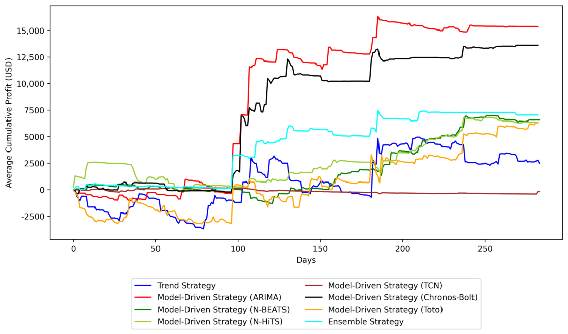
Table A11.
Active Kelly (Section 6.1) trading performance of all trading strategies on the US dollar vs. Chinese Yuan test dataset (1 September 2024 to 31 July 2025) with thresholds. For time series-based approaches, Mean Reversion achieves the highest average cumulative profit and average profit per trade.
Figure A2.
Passive Kelly US dollar vs. Chinese Yuan with thresholds. Average cumulative profit (ACP) trajectories for all trading strategies using passive Kelly (Section 6.1) bet sizing.
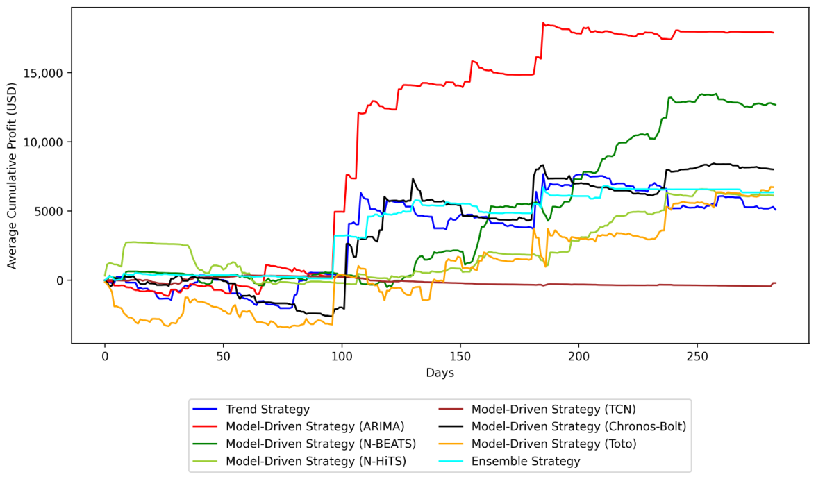
Table A12.
Passive Kelly (Section 6.1) trading performance of all trading strategies on the US dollar vs. Chinese Yuan test dataset (1 September 2024 to 31 July 2025) with thresholds. For time series-based approaches, Mean Reversion achieves the highest average cumulative profit and average profit per trade.
Appendix A.3.2. Fixed Position Size Trading for USD/CNY Using Thresholds
The results for fixed-position-size trading include both pure time-series approaches and news-based approaches.
Figure A3.
US dollar vs. Chinese Yuan. Average Cumulative profit (ACP) trajectories for all trading strategies using fixed bet sizing with thresholds.
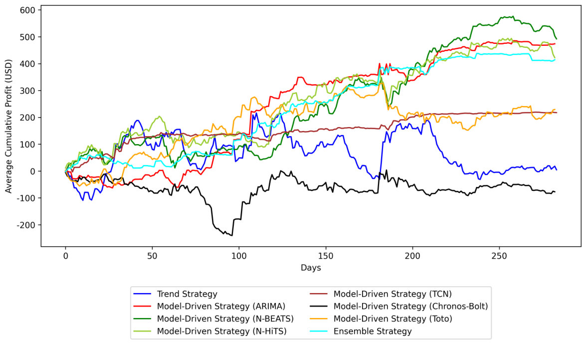
Table A13.
Trading performance of Fixed position size strategy of all time series trading strategies on the USD/CNY test dataset with thresholds. The N-BEATS model has the highest average cumulative profit. The Ensemble model has the highest average profit per trade and Sharpe ratio.
Appendix A.4. Trading Results for USD/BRL Using Thresholds
Appendix A.4.1. Active and Passive Kelly Position Size Trading Results Using Thresholds
Figure A4.
US dollar vs. Brazilian Real. Average cumulative profit (ACP) trajectories for all trading strategies using Active Kelly (Section 6.1) bet sizing with thresholds. Please see the analysis in the text.
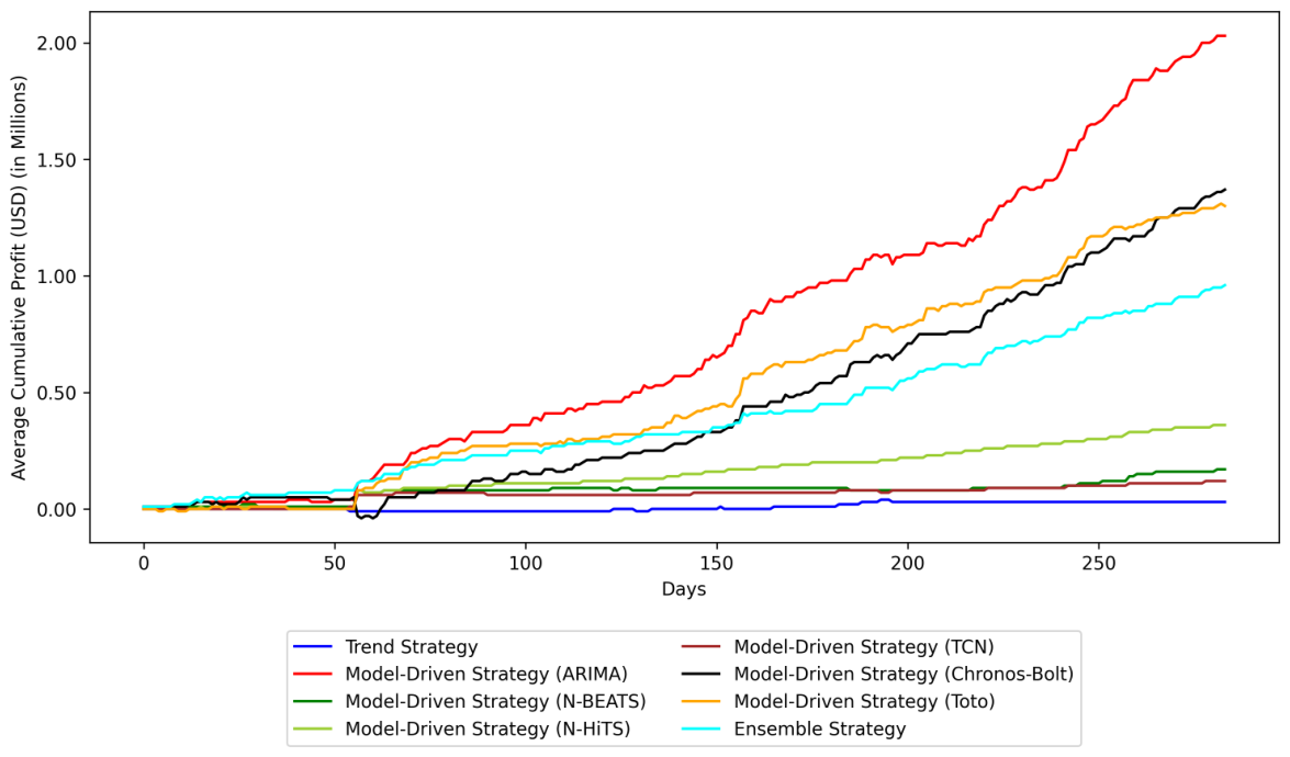
Figure A5.
US dollar vs. Brazilian Real. Average cumulative profit (ACP) trajectories for all trading strategies using Passive Kelly (Section 6.1) bet sizing with thresholds. Please see analysis in text.
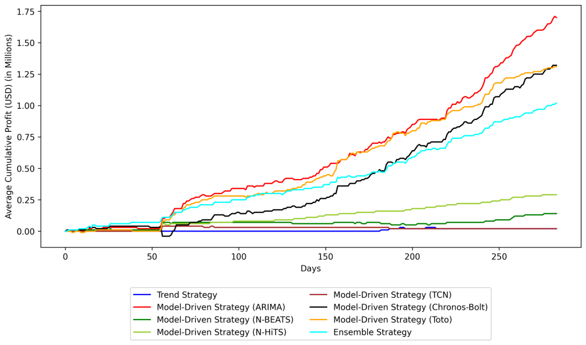
Table A14.
Active Kelly (Section 6.1) trading performance of all trading strategies on the US dollar vs. Brazilian Real test dataset (1 September 2024 to 31 July 2025) with thresholds. For time series approaches, ARIMA achieves the highest average cumulative profit and average profit per trade. The average annualized monthly Sharpe ratio indicates that Ensemble may be a viable trading strategy.
Table A15.
Passive Kelly (Section 6.1) trading performance of all trading strategies on the US dollar vs. Brazilian Real test dataset (1 September 2024 to 31 July 2025) with thresholds. For time series based approaches, the ARIMA achieves the highest average cumulative profit. The average annualized monthly Sharpe ratio indicates that Ensemble may be a viable trading strategy.
Appendix A.4.2. Fixed Position Size Trading Results for USD/BRL Using Thresholds
Figure A6.
Average Cumulative profit (ACP) trajectories for all trading strategies using fixed bet sizing with thresholds. Results are shown for US dollar vs. Brazilian Real.
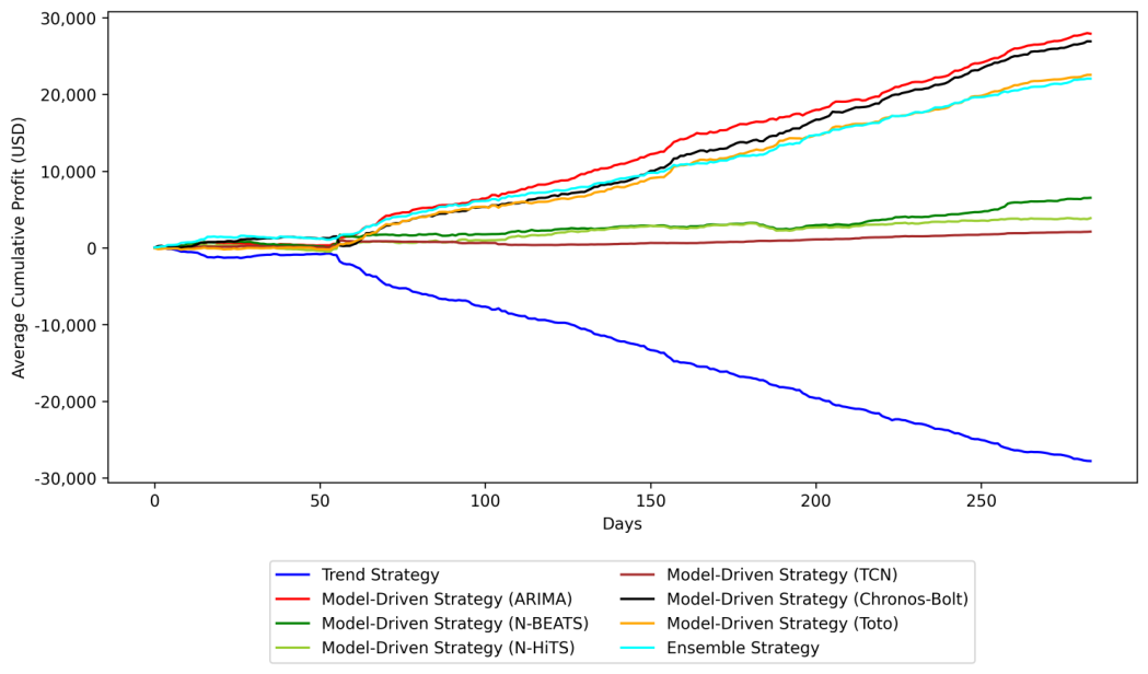
Table A16.
Fixed position size trading performance of all trading strategies on the USD/BRL test dataset with thresholds. ARIMA achieves the highest average cumulative profit and average profit per trade. The average annualized monthly Sharpe ratio and p-value indicate that Ensemble may be a viable trading strategy.
Appendix A.5. Trading Results for USD/GBP Using Thresholds
Appendix A.5.1. Active and Passive Kelly Position Size Trading Results Using Thresholds
Figure A7.
US dollar vs. British Pound. Average cumulative profit (ACP) trajectories for all trading strategies using Active Kelly (Section 6.1) bet sizing with thresholds. Please see the analysis in the text.
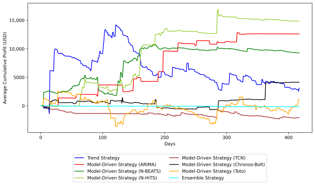
Figure A8.
US dollar vs. British Pound. Average cumulative profit (ACP) trajectories for all trading strategies using Passive Kelly (Section 6.1) bet sizing with thresholds. Please see analysis in text.
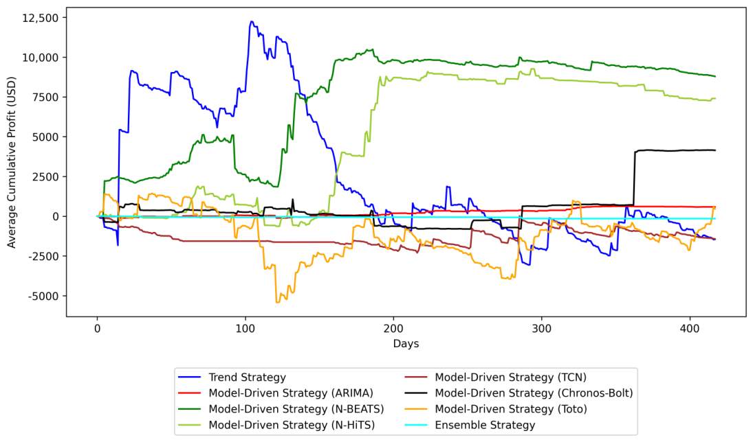
Table A17.
Active Kelly (Section 6.1) trading performance of all trading strategies on the US dollar vs. British Pound test dataset (1 September 2024 to 31 December 2025) with thresholds. For time series approaches, Mean reversion achieves the highest average cumulative profit and average annualized monthly Sharpe ratio.
Table A18.
Passive Kelly (Section 6.1) trading performance of all trading strategies on the US dollar vs. British Pound test dataset (1 September 2024 to 31 December 2025) with thresholds. For time series based approaches, the N-BEATS strategy achieves the highest average cumulative profit. ARIMA achieves the highest average profit per trade and average annualized monthly Sharpe ratio.
Appendix A.5.2. Fixed Position Size Trading Results for USD/GBP Using Thresholds
Figure A9.
Average Cumulative profit (ACP) trajectories for all trading strategies using fixed bet sizing with thresholds. Results are shown for US dollar vs. British Pound.
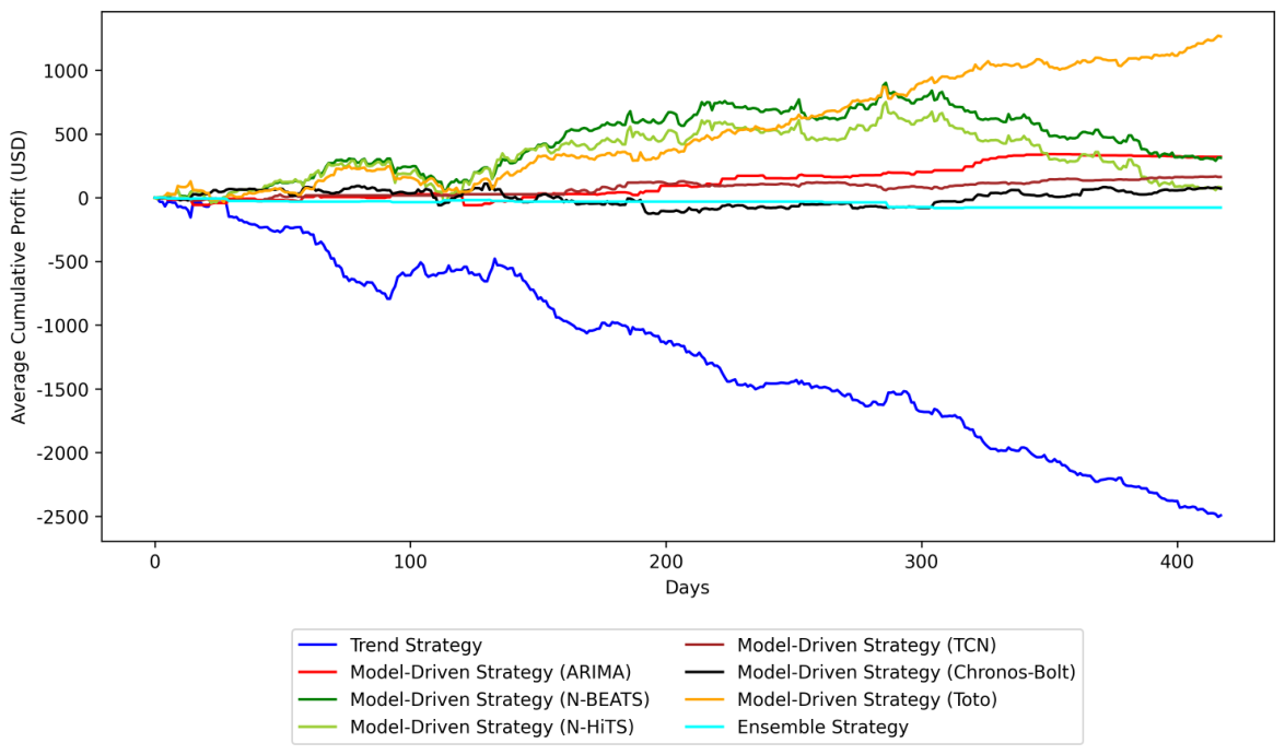
Table A19.
Fixed position size trading performance of all trading strategies on the USD/GBP test dataset with thresholds. Mean Reversion achieves the highest average cumulative profit and Sharpe ratio.
Appendix A.6. Trading Results for USD/EUR Using Thresholds
Appendix A.6.1. Active and Passive Kelly Position Size Trading Results Using Thresholds
Figure A10.
US dollar vs. European Euro. Average cumulative profit (ACP) trajectories for all trading strategies using Active Kelly (Section 6.1) bet sizing with thresholds. Please see the analysis in the text.
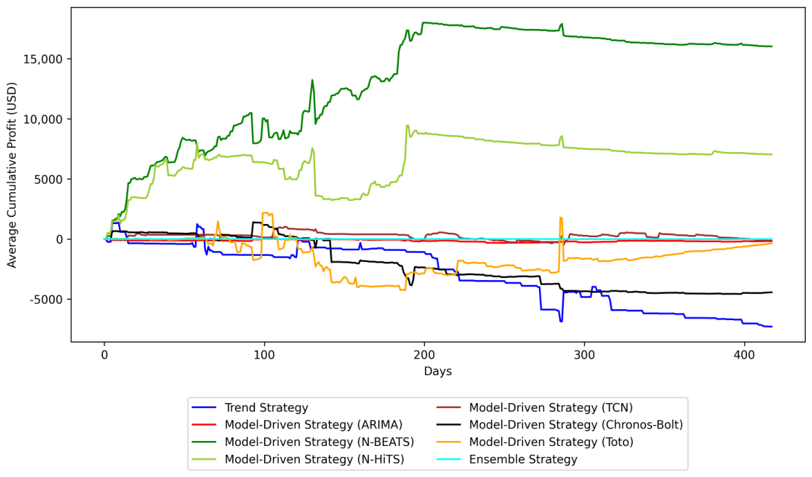
Figure A11.
US dollar vs. European Euro. Average cumulative profit (ACP) trajectories for all trading strategies using Passive Kelly (Section 6.1) bet sizing with thresholds. Please see analysis in text.
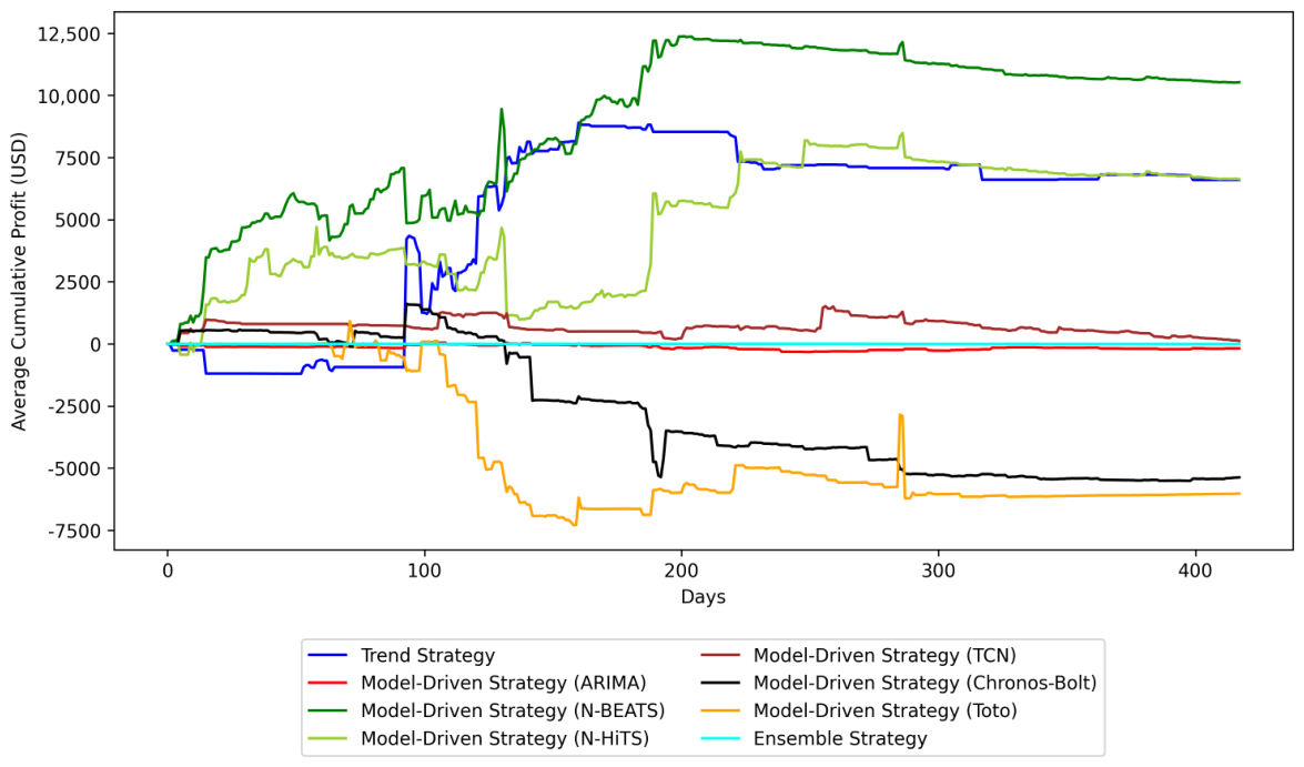
Table A20.
Active Kelly (Section 6.1) trading performance of all trading strategies on the US dollar vs. Euro test dataset (1 September 2024 to 31 December 2025) with thresholds. For time series based approaches, Mean Reversion achieves the highest average cumulative profit, average profit per trade, and annualized average monthly Sharpe ratio .
Table A21.
Passive Kelly (Section 6.1) trading performance of all trading strategies on the US dollar vs. Euro test dataset (1 September 2024 to 31 December 2025). For time series based approaches, the Mean Reversion strategy achieves the highest average cumulative profit per trade and annualized average monthly Sharpe ratio . Trend achieves the highest average profit per trade.
Appendix A.6.2. Fixed Position Size Trading Results for USD/EUR Using Thresholds
Figure A12.
Average Cumulative profit (ACP) trajectories for all trading strategies using fixed bet sizing with thresholds. Results are shown for US dollar vs. Euro.
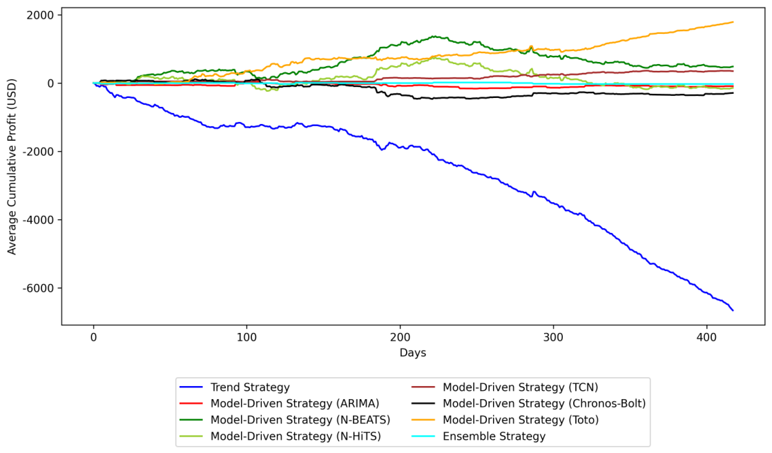
Table A22.
Fixed position size trading performance of all trading strategies on the USD/EUR test dataset with thresholds. Mean reversion achieves the highest average cumulative profit, average profit per trade, and annualized average monthly Sharpe ratio .
Appendix A.6.3. Note on Identical Active and Passive Kelly Results for USD/EUR Using Thresholds
Table A20 and Table A21 show identical average cummulative profit values for some strategies under both Active and Passive Kelly. This is a direct consequence of the positive threshold applied in this appendix. The threshold filters out all predicted moves below a minimum size, which reduces the number of executed trades so severely that the Kelly criterion never fully activates. Specifically, the implementation requires a minimum number of completed trades within the rolling window of d days before switching from the fixed warm-up fraction to the dynamic Kelly fraction (Section 6). When the threshold is high, this minimum is never reached: the d-day window expires and resets the accumulated win/loss statistics before enough trades have occurred. As a result, the Kelly fraction remains at throughout the entire test period. Since the only difference between Active and Passive Kelly lies in how is estimated from trade history, and no such history accumulates here, both variants reduce to the same fixed fraction and produce identical results. This phenomenon is specific to USD/EUR under positive thresholds and does not arise in the zero-threshold results reported in Section 16, where trade frequency is sufficient to activate the dynamic Kelly fraction.
Appendix B. Prompt Templates
Appendix B.1. Expert Prompt for CNY Exchange Rate
The Expert prompt’s construction follows a fixed, explicit sequence. First, a role is specified to establish the model’s standpoint and expected voice. Second, a task is defined to delimit the objective and scope of the response. Third, background information is provided in the form of abbreviations to standardize terminology and reduce ambiguity. Finally, multiple examples are appended, including news items mapped to corresponding labels and lexical cues in which specific words trigger specific labels. These elements are then combined to form the Expert prompt, integrating role specification, task definition, abbreviation-based background, and example-driven guidance into a single, deployable instruction.
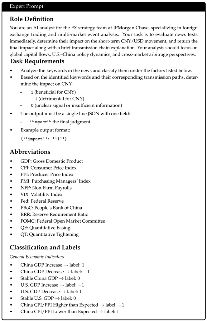
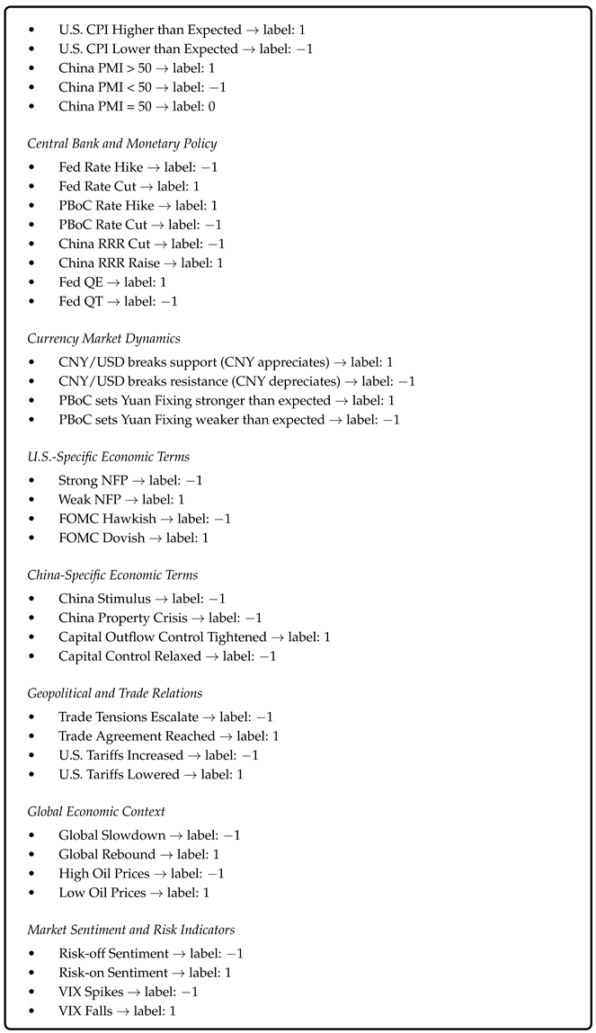
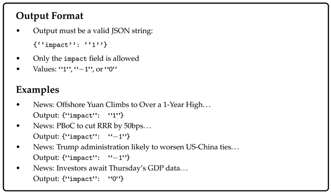
Appendix B.2. Expert Prompt for BRL Without Examples
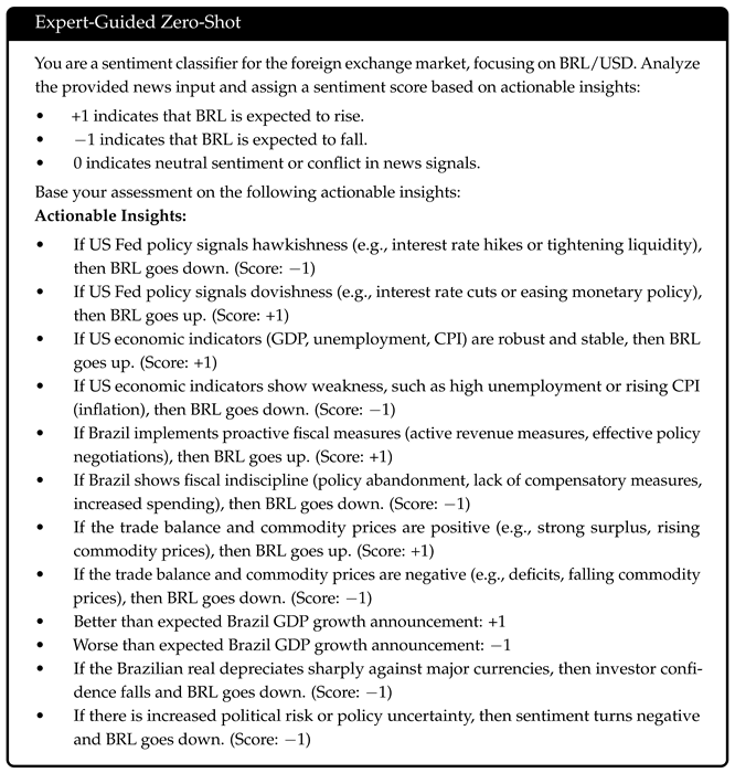
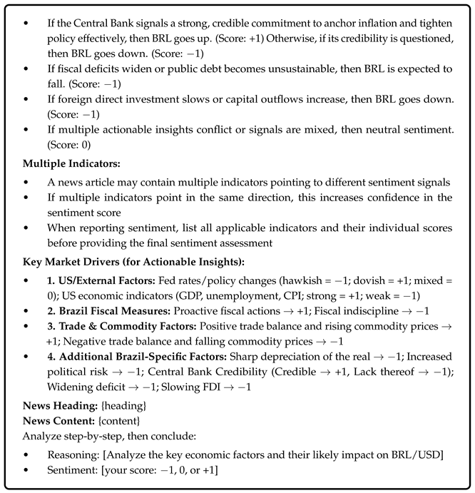
Appendix B.3. Expert Prompt for BRL with Examples
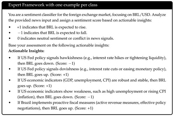
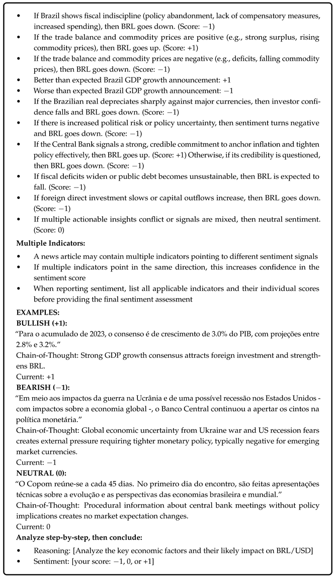
Appendix B.4. Ballinari and Maly Prompt
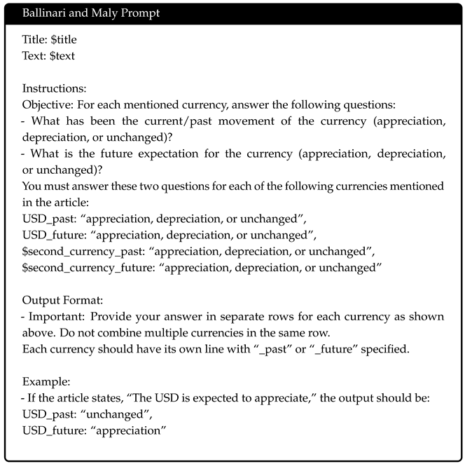
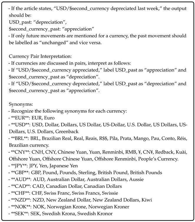
Appendix C. Optimal Kelly Parameters via Grid Search
Table A23, Table A24, Table A25, Table A26, Table A27, Table A28, Table A29 and Table A30 report the optimal Kelly parameters selected via grid search on the validation set for the Active and Passive Kelly strategies, respectively, for each model and currency pair.
Table A23.
Optimal Active Kelly parameters and corresponding average cumulative profit on the validation set (1 July 2024 to 31 August 2024) for USD/CNY. Here, d denotes the rolling window size (days), N the warm-up length (number of trades), and the initial fixed betting fraction used during the warm-up period (see Section 6.1). Trend with achieves the highest average cumulative profit.
Table A24.
Optimal Passive Kelly parameters and corresponding average cumulative profit on the validation set (1 July 2024 to 31 August 2024) for USD/CNY. Column definitions follow Table A23. Trend with achieves the highest average cumulative profit.
Table A25.
Optimal Active Kelly parameters and corresponding average cumulative profit on the validation set (1 July 2024 to 31 August 2024) for USD/BRL. Column definitions follow Table A23. Chronos–Bolt with achieves the highest average cumulative profit.
Table A26.
Optimal Passive Kelly parameters and corresponding average cumulative profit on the validation set (1 July 2024 to 31 August 2024) for USD/BRL. Column definitions follow Table A23. Chronos–Bolt with achieves the highest average cumulative profit.
Table A27.
Optimal Active Kelly parameters and corresponding average cumulative profit on the validation set (1 July 2024 to 31 August 2024) for USD/GBP. Column definitions follow Table A23. ARIMA with achieves the highest average cumulative profit.
Table A28.
Optimal Passive Kelly parameters and corresponding average cumulative profit on the validation set (1 July 2024 to 31 August 2024) for USD/GBP. Column definitions follow Table A23. Moving Avg. Crossover with achieves the highest average cumulative profit.
Table A29.
Optimal Active Kelly parameters and corresponding average cumulative profit on the validation set (1 July 2024 to 31 August 2024) for USD/EUR. Column definitions follow Table A23. Ensemble with achieves the highest average cumulative profit.
Table A30.
Optimal Passive Kelly parameters and corresponding average cumulative profit on the validation set (1 July 2024 to 31 August 2024) for USD/EUR. Column definitions follow Table A23. Mean Reversion with achieves the highest average cumulative profit.
References
- Triennial Central Bank Survey of Foreign Exchange and Over-the-Counter (OTC) Derivatives Markets in 2022. 2022. Available online: https://www.bis.org/statistics/rpfx22.htm (accessed on 10 January 2026).
- Box, G.E.; Jenkins, G.M.; Reinsel, G.C.; Ljung, G.M. Time Series Analysis: Forecasting and Control; John Wiley & Sons: Hoboken, NJ, USA, 2015. [Google Scholar]
- von Beschwitz, B. Internationalization of the Chinese Renminbi: Progress and Outlook; FEDS Notes; Board of Governors of the Federal Reserve System: Washington, DC, USA, 2024; pp. 30–33. [Google Scholar]
- Granger, C.W.; Joyeux, R. An introduction to long-memory time series models and fractional differencing. J. Time Ser. Anal. 1980, 1, 15–29. [Google Scholar]
- Hosking, J. Fractional differencing. Biometrika 1981, 68, 165–176. [Google Scholar]
- Beran, J. Statistics for Long-Memory Processes; Routledge: London, UK, 2017. [Google Scholar]
- Baillie, R.T. Long memory processes and fractional integration in econometrics. J. Econom. 1996, 73, 5–59. [Google Scholar] [CrossRef] [Scilit]
- Hadad, E.; Hodarkar, S.; Lemeneh, B.; Shasha, D. Machine Learning-Enhanced Pairs Trading. Forecasting 2024, 6, 434–455. [Google Scholar] [CrossRef] [Scilit]
- Oreshkin, B.N.; Carpov, D.; Chapados, N.; Bengio, Y. N-BEATS: Neural basis expansion analysis for interpretable time series forecasting. arXiv 2019, arXiv:1905.10437. [Google Scholar] [CrossRef] [Scilit]
- Challu, C.; Olivares, K.G.; Oreshkin, B.N.; Ramirez, F.G.; Canseco, M.M.; Dubrawski, A. Nhits: Neural hierarchical interpolation for time series forecasting. Proc. AAAI Conf. Artif. Intell. 2023, 37, 6989–6997. [Google Scholar] [CrossRef] [Scilit]
- Lea, C.; Flynn, M.D.; Vidal, R.; Reiter, A.; Hager, G.D. Temporal convolutional networks for action segmentation and detection. In Proceedings of the IEEE Conference on Computer Vision and Pattern Recognition, Honolulu, HI, USA, 21–26 July 2017; pp. 156–165. [Google Scholar]
- Bai, S.; Kolter, J.Z.; Koltun, V. An empirical evaluation of generic convolutional and recurrent networks for sequence modeling. arXiv 2018, arXiv:1803.01271. [Google Scholar]
- Wan, R.; Mei, S.; Wang, J.; Liu, M.; Yang, F. Multivariate Temporal Convolutional Network: A Deep Neural Networks Approach for Multivariate Time Series Forecasting. Electronics 2019, 8, 876. [Google Scholar] [CrossRef] [Scilit]
- Ansari, A.F.; Stella, L.; Turkmen, C.; Zhang, X.; Mercado, P.; Shen, H.; Shchur, O.; Rangapuram, S.S.; Arango, S.P.; Kapoor, S.; et al. Chronos: Learning the Language of Time Series. arXiv 2024, arXiv:2403.07815. [Google Scholar]
- Cohen, B.; Khwaja, E.; Wang, K.; Masson, C.; Ramé, E.; Doubli, Y.; Abou-Amal, O. Toto: Time Series Optimized Transformer for Observability. arXiv 2024, arXiv:2407.07874. [Google Scholar]
- Fatouros, G.; Soldatos, J.; Kouroumali, K.; Makridis, G.; Kyriazis, D. Transforming sentiment analysis in the financial domain with ChatGPT. Mach. Learn. Appl. 2023, 14, 100508. [Google Scholar] [CrossRef] [Scilit]
- Grattafiori, A.; Dubey, A.; Jauhri, A.; Pandey, A.; Kadian, A.; Al-Dahle, A.; Letman, A.; Mathur, A.; Schelten, A.; Vaughan, A.; et al. The Llama 3 Herd of Models. arXiv 2024, arXiv:2407.21783. [Google Scholar]
- Ballinari, D.; Maly, J. FX Sentiment Analysis with Large Language Models; Working Papers 2025-11; Swiss National Bank: Zurich, Switzerland, 2025. [Google Scholar]
- Massive. Massive: Real-Time and Historical Market Data APIs. 2025. Available online: https://massive.com (accessed on 29 August 2025).
- Bloomberg, L.P. Bloomberg Terminal. 2026. Available online: https://www.bloomberg.com/professional/solution/bloomberg-terminal/ (accessed on 15 January 2026).
- London Stock Exchange Group and Thomson Reuters. LSE Thomson Reuters Newswire Service. 2025. Available online: https://www.lseg.com/en/data-analytics/financial-news-service (accessed on 29 August 2025).
- Brock, W.; Lakonishok, J.; LeBaron, B. Simple technical trading rules and the stochastic properties of stock returns. J. Financ. 1992, 47, 1731–1764. [Google Scholar] [CrossRef] [Scilit]
- Acharya, P. An R-Based Analysis of a Moving Average Crossover Strategy vs. Buy-and-Hold: Evidence from Several Major Tech Stocks. SSRN Working Paper 2025. Epub ahead of printing. [Google Scholar] [CrossRef] [Scilit]
- Akiba, T.; Sano, S.; Yanase, T.; Ohta, T.; Koyama, M. Optuna: A Next-generation Hyperparameter Optimization Framework. In Proceedings of the 25th ACM SIGKDD International Conference on Knowledge Discovery & Data Mining, Anchorage, AK, USA, 4–8 August 2019; pp. 2623–2631. [Google Scholar]
- Lo, A.W. The Statistics of Sharpe Ratios. Financ. Anal. J. 2002, 58, 36–52. [Google Scholar] [CrossRef] [Scilit]
- Joanes, D.N.; Gill, C.A. Comparing measures of sample skewness and kurtosis. J. R. Stat. Soc. Ser. D (Stat.) 1998, 47, 183–189. [Google Scholar] [CrossRef] [Scilit]
- Efron, B.; Tibshirani, R.J. An Introduction to the Bootstrap; Chapman & Hall/CRC: Boca Raton, FL, USA, 1993. [Google Scholar]
- Good, P. Permutation, Parametric, and Bootstrap Tests of Hypotheses; Springer Series in Statistics; Springer: Berlin/Heidelberg, Germany, 2005. [Google Scholar]
- Kingma, D.P.; Ba, J. Adam: A Method for Stochastic Optimization. arXiv 2017, arXiv:1412.6980. [Google Scholar]
- Araci, D. Finbert: Financial sentiment analysis with pre-trained language models. arXiv 2019, arXiv:1908.10063. [Google Scholar]
- Xu, X.; Wen, F.; Chu, B.; Fu, Z.; Lin, Q.; Liu, J.; Fei, B.; Li, Y.; Zhou, L.; Yang, Z. FinBERT2: A Specialized Bidirectional Encoder for Bridging the Gap in Finance-Specific Deployment of Large Language Models. In Proceedings of the 31st ACM SIGKDD Conference on Knowledge Discovery and Data Mining V.2, KDD ’25, Toronto, ON, Canada, 3–7 August 2025; pp. 5117–5128. [Google Scholar] [CrossRef] [Scilit]
- Leme, L. FinBERT-PT-BR: Financial BERT for Brazilian Portuguese. 2023. Available online: https://huggingface.co/lucas-leme/FinBERT-PT-BR (accessed on 15 January 2024).
- Hu, Z.; Rostami, M.; Thomason, J. Expert Personas Improve LLM Alignment but Damage Accuracy: Bootstrapping Intent-Based Persona Routing with PRISM. arXiv 2026, arXiv:2603.18507. [Google Scholar]
- Hochreiter, S.; Schmidhuber, J. Long Short-Term Memory. Neural Comput. 1997, 9, 1735–1780. [Google Scholar] [CrossRef] [Scilit] [PubMed]
- Fischer, T.; Krauss, C. Deep learning with long short-term memory networks for financial market predictions. Eur. J. Oper. Res. 2018, 270, 654–669. [Google Scholar] [CrossRef] [Scilit]
- Vaswani, A.; Shazeer, N.; Parmar, N.; Uszkoreit, J.; Jones, L.; Gomez, A.N.; Kaiser, Ł.; Polosukhin, I. Attention is all you need. In Proceedings of the 31st Conference on Neural Information Processing Systems (NIPS 2017), Long Beach, CA, USA, 4–9 December 2017; Volume 30. [Google Scholar]
- Devlin, J.; Chang, M.W.; Lee, K.; Toutanova, K. Bert: Pre-training of deep bidirectional transformers for language understanding. In Proceedings of the 2019 Conference of the North American Chapter of the Association for Computational Linguistics: Human Language Technologies, Volume 1 (Long and Short Papers), Minneapolis, MN, USA, 2–7 June 2019; pp. 4171–4186. [Google Scholar]
- Radford, A.; Narasimhan, K.; Salimans, T.; Sutskever, I. Improving Language Understanding by Generative Pre-Training. 2018. Available online: https://www.mikecaptain.com/resources/pdf/GPT-1.pdf (accessed on 15 January 2026).
- Liu, X.Y.; Wang, G.; Yang, H.; Zha, D. Fingpt: Democratizing internet-scale data for financial large language models. arXiv 2023, arXiv:2307.10485. [Google Scholar]
- Sezer, O.B.; Gudelek, M.U.; Ozbayoglu, A.M. Financial time series forecasting with deep learning: A systematic literature review: 2005–2019. Appl. Soft Comput. 2020, 90, 106181. [Google Scholar] [CrossRef] [Scilit]
- Raffel, C.; Shazeer, N.; Roberts, A.; Lee, K.; Narang, S.; Matena, M.; Zhou, Y.; Li, W.; Liu, P.J. Exploring the Limits of Transfer Learning with a Unified Text-to-Text Transformer. arXiv 2023, arXiv:1910.10683. [Google Scholar]
- Das, A.; Kong, W.; Sen, R.; Zhou, Y. A decoder-only foundation model for time-series forecasting. arXiv 2023, arXiv:2310.10688. [Google Scholar]
- Zuo, Z.; Liu, Z.; Zheng, Z.; Huang, Z.; Zhu, S.; Yu, Z.; Kwok, J.T. AutoTimes: A foundation model for time-series forecasting. arXiv 2024, arXiv:2401.12345. [Google Scholar]
- Nie, Y.; Nguyen, N.H.; Sinthong, P.; Kalagnanam, J. A Time Series is Worth 64 Words: Long-term Forecasting with Transformers. arXiv 2023, arXiv:2211.14730. [Google Scholar]
- Cohen, B.; Khwaja, E.; Doubli, Y.; Lemaachi, S.; Lettieri, C.; Masson, C.; Miccinilli, H.; Ramé, E.; Ren, Q.; Rostamizadeh, A.; et al. This Time is Different: An Observability Perspective on Time Series Foundation Models. arXiv 2025, arXiv:2505.14766. [Google Scholar]
- Loughran, T.; McDonald, B. When is a liability not a liability? Textual analysis, dictionaries, and 10-Ks. J. Financ. 2011, 66, 35–65. [Google Scholar]
- Nassirtoussi, A.K.; Aghabozorgi, S.; Wah, T.Y.; Ngo, D.C.L. Text mining for market prediction: A systematic review. Expert Syst. Appl. 2014, 41, 7653–7670. [Google Scholar] [CrossRef] [Scilit]
- Jeon, Y.; McCurdy, T.H.; Zhao, X. News as sources of jumps in stock returns: Evidence from 21 million news articles for 9000 companies. J. Financ. Econ. 2022, 145, 1–17. [Google Scholar] [CrossRef] [Scilit]
- Tetlock, P.C. Giving content to investor sentiment: The role of media in the stock market. J. Financ. 2007, 62, 1139–1168. [Google Scholar] [CrossRef] [Scilit]
- Zhang, W.; Skiena, S. Trading strategies to exploit blog and news sentiment. Proc. Int. AAAI Conf. Web Soc. Media 2010, 4, 375–378. [Google Scholar] [CrossRef] [Scilit]
- Ding, X.; Zhang, Y.; Liu, T.; Duan, J. Deep learning for event-driven stock prediction. In Proceedings of the International Joint Conference on Artificial Intelligence, Buenos Aires, Argentina, 25–31 July 2015; Volume 15, pp. 2327–2333. [Google Scholar]
- Fama, E.F. Efficient capital markets: A review of theory and empirical work. J. Financ. 1970, 25, 383–417. [Google Scholar] [CrossRef] [Scilit]
- Anil, K.; Neha. Testing the Weak Form Efficient Market Hypothesis: An Interpretive Study of Market Efficiency Via Literary Logic and Evidence. J. Glob. Econ. Manag. Bus. Res. 2025, 17, 26–36. [Google Scholar] [CrossRef] [Scilit]
- Lo, A.W. The adaptive markets hypothesis: Market efficiency from an evolutionary perspective. J. Portf. Manag. 2004, 15–29. [Google Scholar] [CrossRef] [Scilit]
- Shleifer, A.; Vishny, R.W. The limits of arbitrage. J. Financ. 1997, 52, 35–55. [Google Scholar] [CrossRef] [Scilit]
- Meese, R.A.; Rogoff, K. Empirical exchange rate models of the seventies: Do they fit out of sample? J. Int. Econ. 1983, 14, 3–24. [Google Scholar]
- Engel, C.; West, K.D. Exchange rates and fundamentals. J. Political Econ. 2005, 113, 485–517. [Google Scholar] [CrossRef] [Scilit]
- Fama, E.F. Efficient capital markets: II. J. Financ. 1991, 46, 1575–1617. [Google Scholar] [CrossRef] [Scilit]
- Grossman, S.J.; Stiglitz, J.E. On the impossibility of informationally efficient markets. Am. Econ. Rev. 1980, 70, 393–408. [Google Scholar]
- Pellicani, A.; Pio, G.; Ceci, M. CARROT: Simultaneous prediction of anomalies from groups of correlated cryptocurrency trends. Expert Syst. Appl. 2025, 260, 125457. [Google Scholar] [CrossRef] [Scilit]
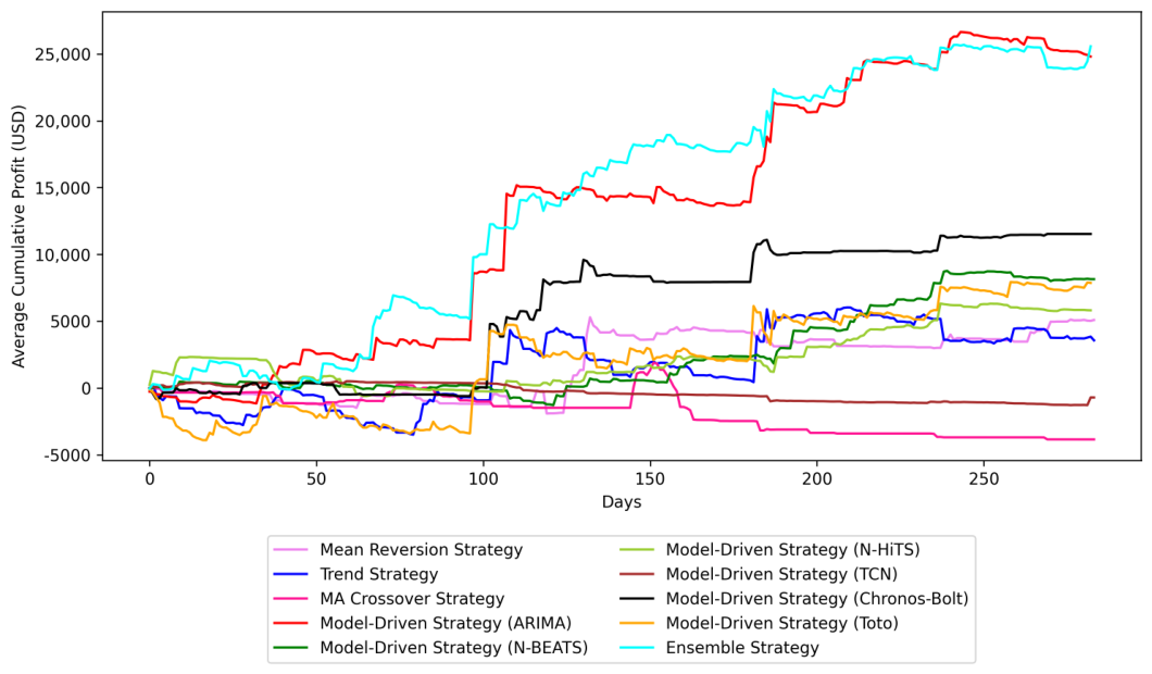
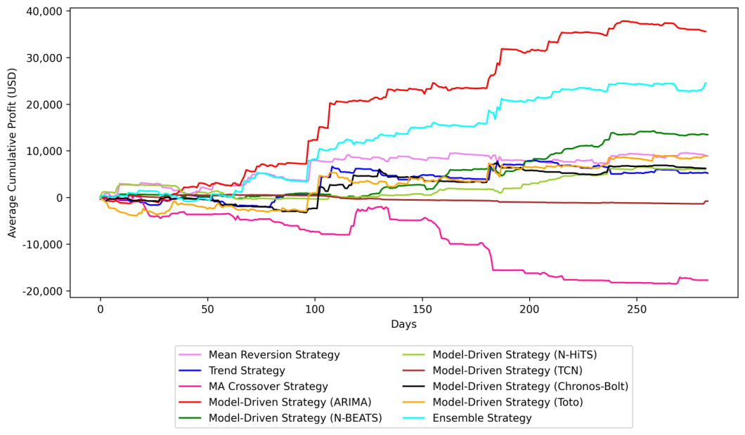
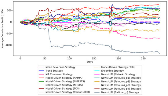
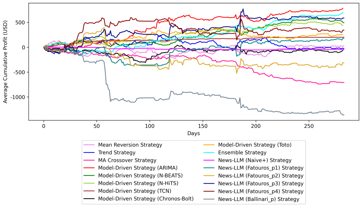
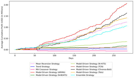
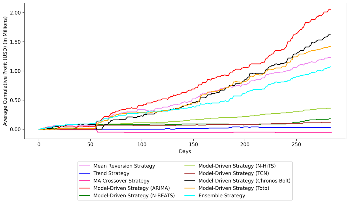
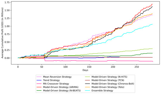
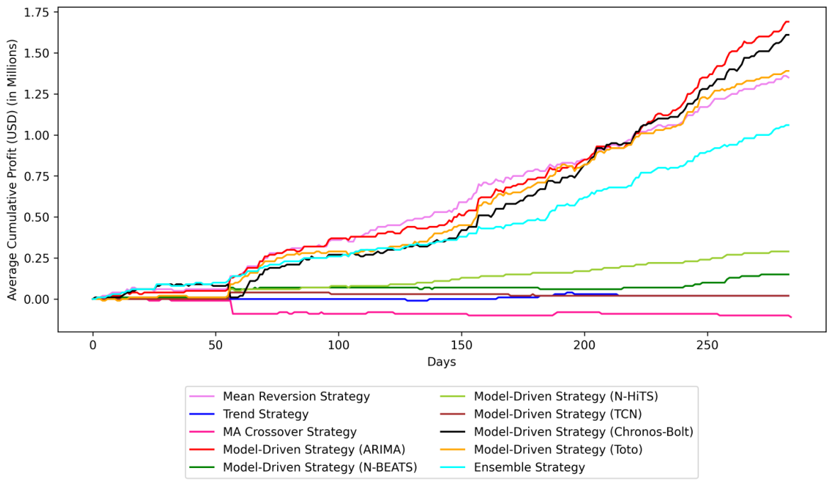
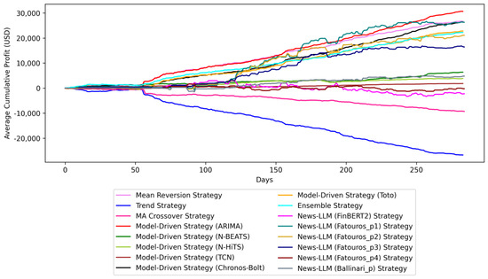
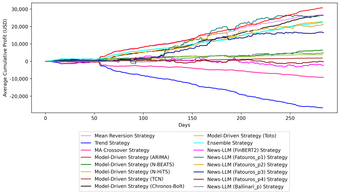
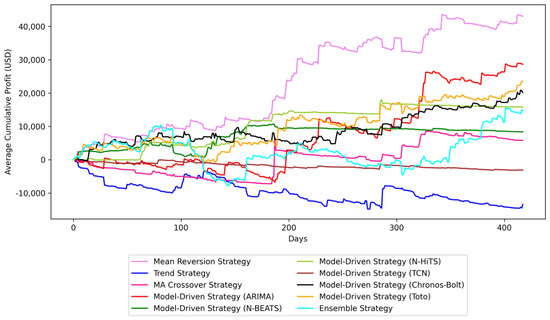
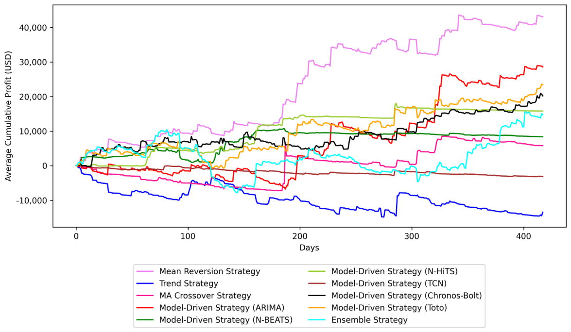
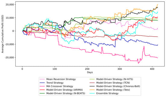
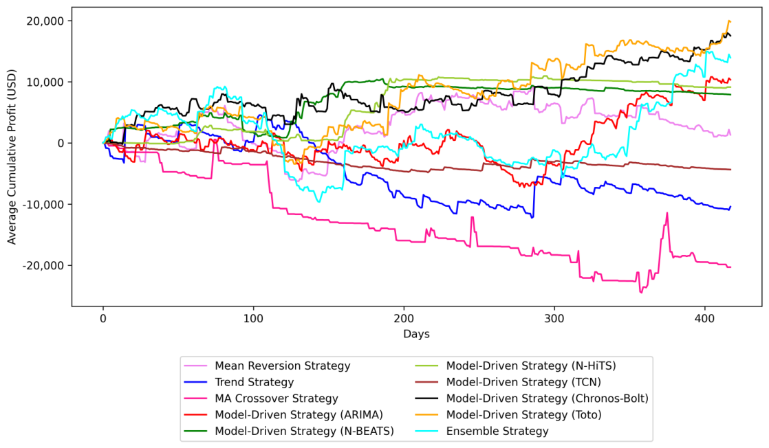
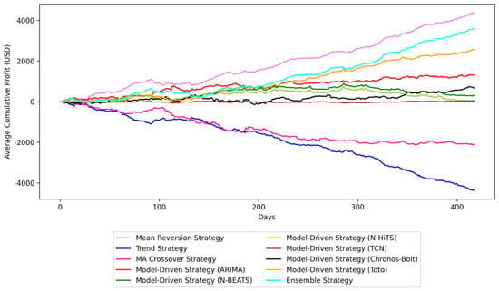
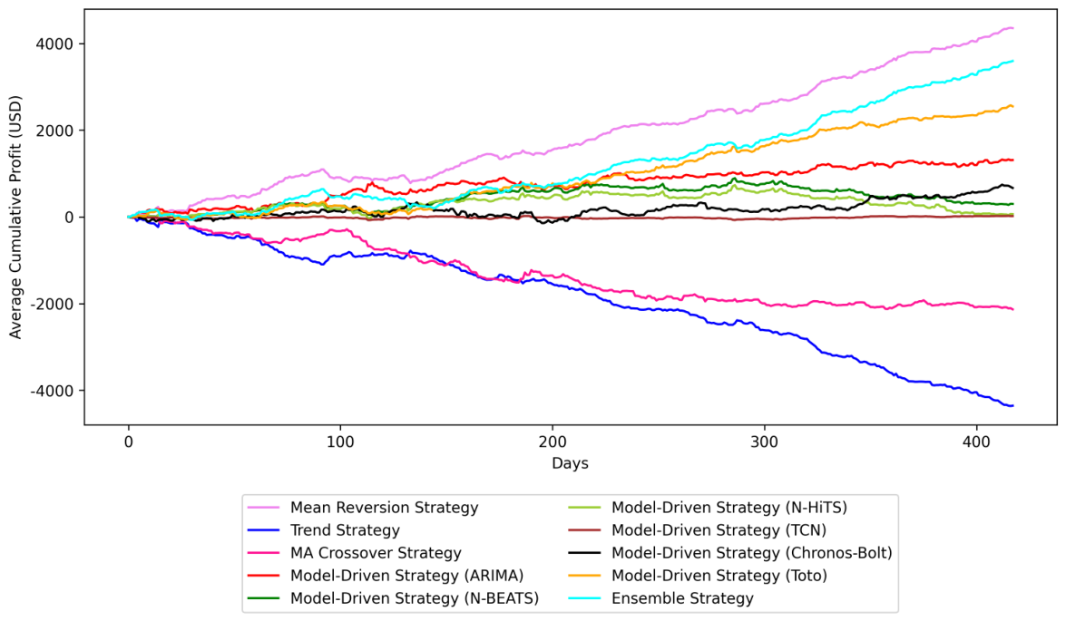
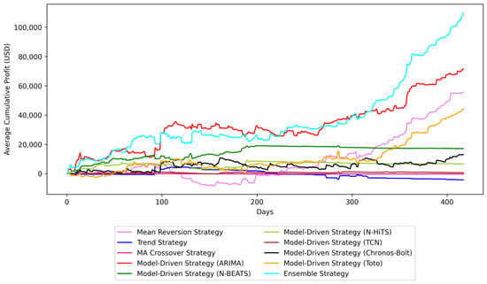
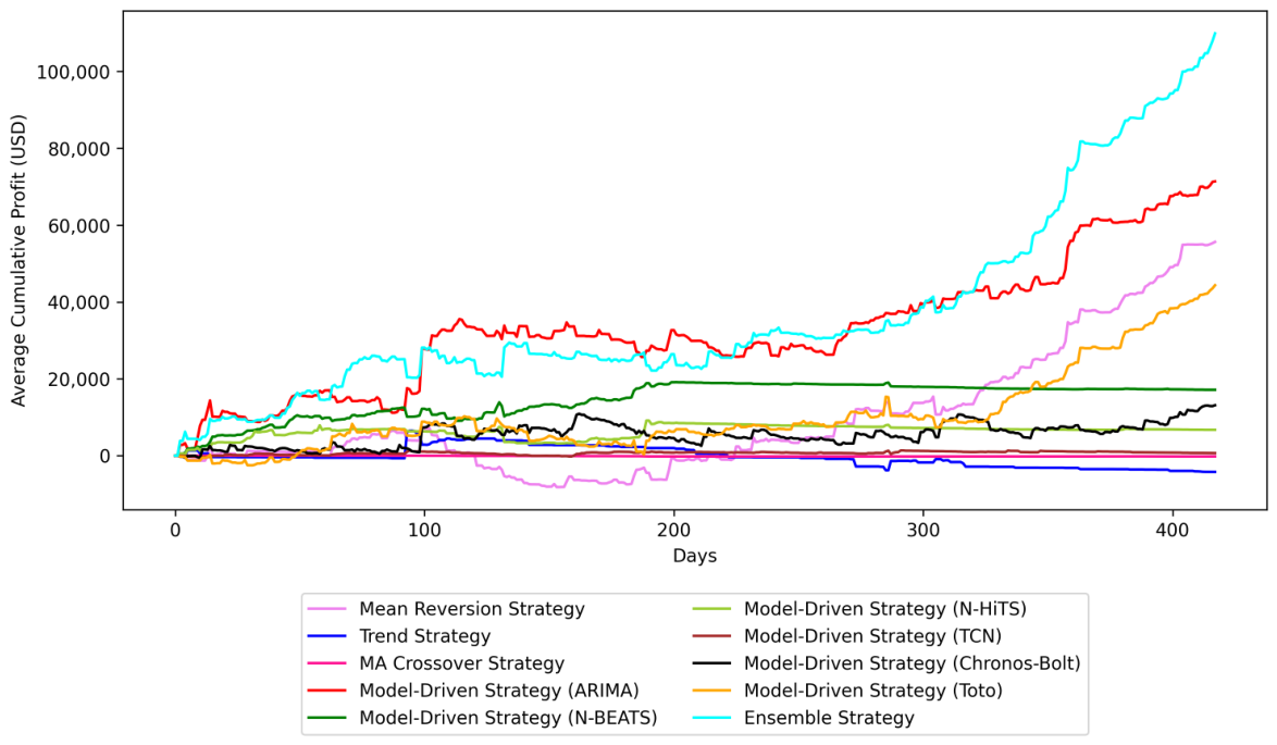
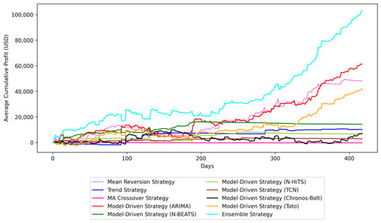
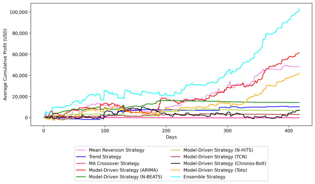
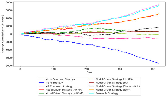
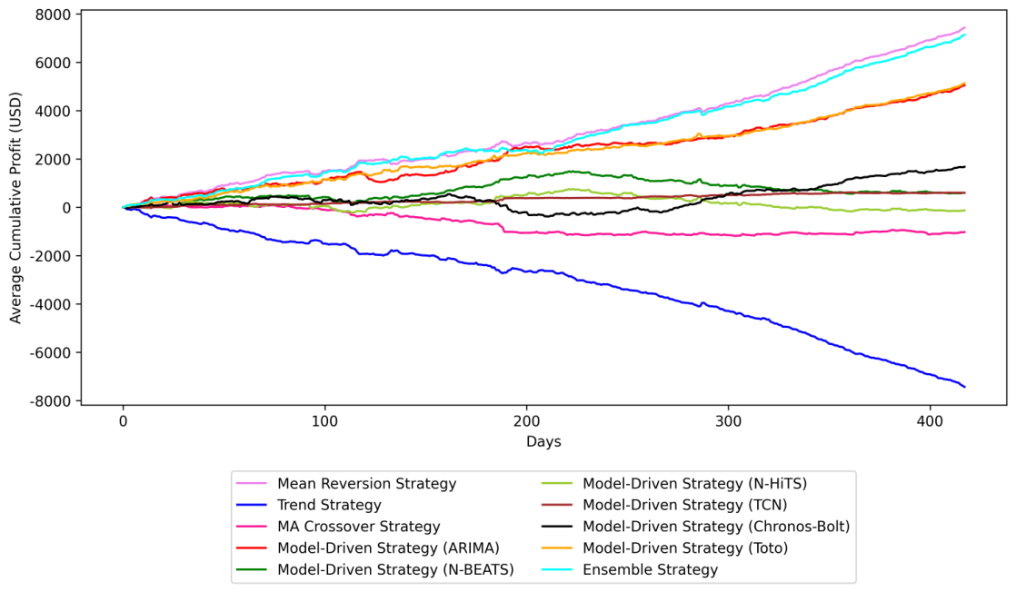

Disclaimer/Publisher’s Note: The statements, opinions and data contained in all publications are solely those of the individual author(s) and contributor(s) and not of MDPI and/or the editor(s). MDPI and/or the editor(s) disclaim responsibility for any injury to people or property resulting from any ideas, methods, instructions or products referred to in the content. |
© 2026 by the authors. Licensee MDPI, Basel, Switzerland. This article is an open access article distributed under the terms and conditions of the Creative Commons Attribution (CC BY) license.