Simulation of Signed Probability Distributions ^†

Abstract

The notion of negative probability is almost one hundred years old, and so far, some results have been obtained in the direction of the theoretical development of the notion of extended probability. However, there is still a strong need for computational methods and tools, and the presented article is aimed at filling this gap. Several examples, including Feynman’s problem, of the numerical simulation of signed probability distributions are provided for the first time, along with the results of the simulation using the developed software toolbox. The presented methods and results might open wide possibilities for using signed probabilities in the fields of quantum computing, decision making, finance, insurance, large language models and artificial intelligence, and other fields where the use of signed probability distributions can extend the current level of mathematical modeling.

1. Introduction: History and Motivation

One can hardly imagine today’s mathematics without using negative numbers. However, in the case of probability theory, the use of negative probabilities is currently very limited.

One reason for that is the problem of the interpretation of negative probabilities—but the problem of the interpretation and acceptance of negative numbers was not easier. Focusing only on the development of European mathematics, let us recall [1] that Michael Stifel wrote about negative numbers as absurd numbers; Gerolamo Cardano considered negative roots of equations impossible solutions and called them fictitious; Franciscus Vieta discarded negative numbers entirely; Blaise Pascal regarded the subtraction of four from zero as total nonsense.

In the context of this article, the approach of René Descartes is worth special attention. He called negative roots of equations false, because they represent numbers less than nothing. However, he demonstrated that, given an equation, one can obtain another equation (and, actually, an infinite number of such equations) whose roots are larger than the roots of the original equation by any given quantity, which means that an equation with negative roots could be transformed into an equation with positive roots. Because of this, Descartes inclined to accept the notion of a negative number [1].

The history of negative probability repeats, in some sense, the history of negative numbers. The need to solve important challenging problems often leads to entering previously unknown grounds and exploring them without hesitation. The notion of negative probability appeared first in quantum mechanics, and three great physicists, all Nobel laureates, contributed to that.

In 1932, Eugene Wigner wrote [2] about using negative probabilities in intermediate derivations:

“Of course $P(x_1,\dots x_n;p_1,\dots ,p_n)$ cannot be really interpreted as the simultaneous probability for coordinates and momenta, as is clear from the fact that it may take negative values. But, of course, this must not hinder the use of it in calculations as an auxiliary function which obeys many relations we would expect from such a probability.”

In his Bakerian lecture, given in 1940 and published in 1942, Paul Dirac provided an extended discussion on negative energies and negative probabilities, and seconded to Wigner [3]:

“Negative energies and probabilities should not be considered as nonsense. They are well-defined concepts mathematically, like a negative sum of money, since the equations which express the important properties of energies and probabilities can still be used when they are negative. Thus negative energies and probabilities should be considered simply as things which do not appear in experimental results.”

In 1987, Richard Feynman [4] also discussed the notion of negative probability and even provided an illustrative example with conditional probabilities, which is one of the examples of numerical simulation in this paper. Feynman wrote that

“A probability greater than unity presents no problem different from that of negative probabilities”,

because they both are used in intermediate computations, and the final result is always expressed as a positive number between zero and one.

The lecture by Paul Dirac, who was a Lucasian Professor at the University of Cambridge, provided motivation to Maurice Bartlett, who was also a professor at Cambridge, for writing the first mathematical paper [5] on negative probability and creating its theoretical foundation.

“It has been shown that orthodox probability theory may consistently be extended to include probability numbers outside the conventional range, and in particular negative probabilities.”

“Negative probabilities must always be combined with positive ones to give an ordinary probability before a physical interpretation is admissible.”

“…a negative probability implies automatically a complementary probability greater than unity.”

Bartlett also introduced the notion of “extraordinary random variables” and their signed probability-generating functions:

“Random variables are correspondingly generalized to include extraordinary random variables; these have been defined in general, however, only through their characteristic functions.”

Bartlett’s work inspired some further theoretical explorations aimed at the development of a general theory of extended probability, such as in [6,7,8,9,10,11].

Naturally, there were also attempts of interpretation of the notion of negative probability [12,13,14,15,16]. However, the interpretations of signed probability distributions still did not receive proper attention.

There are interesting works on the applications of negative probability in finance by Haug [17] and by Burgin and Meissner [18,19]. Some ideas for applications have been collected by Blass and Gurevich [20].

And here we come to the important reason for the current limited use of negative probabilities: there are some theoretical developments, but there is a total lack of suitable computational tools. A demonstration of how simulations of signed (or extended) probability distributions can be done is the main motivation for the present paper.

The first steps in this direction were made only very recently by Leonenko and Podlubny. In the work [21], the Monte Carlo method for numerical differentiation of non-integer order has been developed (73 years after the publication of the Monte Carlo method for integration in [22]), and in the papers [23,24], the signed probability distributions (generalized Sibuya distribution) were used for the numerical evaluation of fractional-order derivatives. In the case of fractional-order differentiation, the number of sign changes in the probability-generating function of the generalized Sibuya distribution is finite, and it was possible to use this to reduce the problem of the simulation of ordinary probability distributions with non-negative probabilities.

In the present article, several new types of examples of numerical simulation of signed probability distributions are presented. In particular, for the first time, a numerical simulation of the famous Richard Feynman example is provided. These examples of simulations provide additional light on how we can understand signed probability distributions.

2. Example 1: Partial Coins

The first-ever example of the numerical simulation of a signed probability distribution with an infinite number of sign changes (“half of a coin”, or a half-coin) has been provided by Leonenko and Podlubny only in 2025 [25], exactly 20 years after a half-coin was introduced in 2005 theoretically by G. Székely [26]. A “half-coin” is not a physical half of a round metal disk still having two sides, but a random variable taking an infinite number of values—some with positive probabilities, some with negative probabilities, alternating.

A partial $\mu$-coin is defined using its probability-generating function

$$f\left(x\right)={\left({\displaystyle \frac{1+x}{2}}\right)}^{\mu }=2^{-\mu }{\displaystyle \sum _{m=0}^{\infty }}{p}_m{x}^m,\mu \in (0,1),$$

(1)

where the coefficients $p_m=\left({\displaystyle \genfrac{}{}{0pt}{}{\mu }{m}}\right)$ have alternating signs starting from $m=1$:

$$p_0>0,p_1>0,p_2<0,p_3>0,p_4<0,p_5>0,p_6<0,\dots$$

The way to the simulation of signed probability distributions, which is in some sense similar to Descartes’ approach to dealing with negative numbers, was indicated by Imre Ruzsa and Gábor Székely [26]:

Theorem 1 

(Ruzsa–Székely [26,27,28]). For every generalized generating function f of a signed probability distribution there exist two generating functions g and h of ordinary non-negative probability distributions such that $fg=h$.

The proof of this theorem can be found in [27] (Theorem 1) or in [28] (Lemma 3.6).

This theorem guarantees the existence of g and h, but not the uniqueness, and it does not provide any method for constructing the functions g and h.

However, if we somehow determine the generating functions for the distributions g and h, then we can do the simulation using the following steps [25]

• Step 1. Expand the probability-generating functions g and h into power series, and compute their coefficients.
• Step 2. Using the coefficients of the power series, compute the cumulated mass distribution functions $G\left(x\right)$ and $H\left(x\right)$.
• Step 3. Generate a set of uniformly distributed points $U_i$ in $(0,1)$.
• Step 4. For each $U_i$ find a pair of the values $G_i$ and $H_i$; for this, the method of the inverse cumulated mass probability function can be used.
• Step 5. The differences of $H_i$ and $G_i$ give the values $F_i=H_i-G_i$ of the simulated signed distribution f.

The beauty consists in the fact that the difference of the outputs of the simultaneous trials of H and G is either zero or one, and simultaneously running two independent copies of a half-coin process produces the same outputs as tossing a normal coin. In ref. [25], this method was used for simulating various types of partial coins (one-third-coins, etc.) and biased partial coins. The key instrument in searching for H and G was the Sibuya distribution [29] and the software tools [30] for its simulation developed earlier [24].

For the $\mu$-coin (0 < $\mu$ < 1) the pairs of suitable ordinary non-negative probability distributions g and h are [25]:

$$g_k\left(x\right)=\left(1-{(1-x)}^{\mu }\right)x^k,$$

(2)

$$h_k\left(x\right)=2^{-\mu }{x}^k\left({(1+x)}^{\mu }-{(1-x^2)}^{\mu }\right),$$

(3)

where k can be $-1,0,1,2,3,4,\dots$ The proof that the probability-generating functions (2) and (3) define the ordinary non-negative probability distributions is given in [25] and can be used for simulating the signed probability distribution given by the probability distribution function (1).

The functions $g_k\left(x\right)$ are given by the generating function of the Sibuya distribution multiplied by $x^k$, and $h_k\left(x\right)$ are the products of $f\left(x\right)$ and $g_k\left(x\right)$.

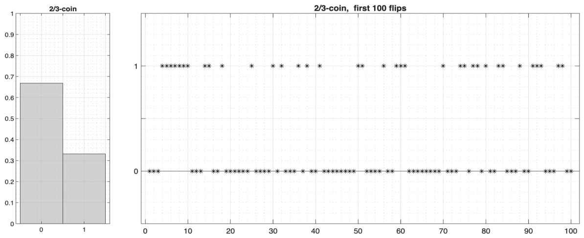
The simulations can be done using the five-step method described above, implemented in the form of a toolbox for MATLAB [31], which can be used for further experiments. The results of one simulation for $\mu ={\displaystyle \frac{2}{3}}$ (a two-thirds-coin) are shown in Figure 1. Other examples of the simulation of partial coins (and biased partial coins) can be found in [25].

3. Example 2

Let us consider a signed probability distribution f with the following generating function, which is not an infinite series, but a polynomial:

$$f\left(x\right)=1-{\displaystyle \frac{1}{2}}x+{\displaystyle \frac{1}{2}}{x}^2.$$

(4)

The support of f is $\{0,1,2\}$, with $p_0=1$, $p_1=-0.5$, and $p_2=0.5$. Obviously, $p_0+p_1+p_2=1$, and formally using the standard formula for the expectation, we have

$$\mathbb{E}\left(f\right)=1·0+(-0.5)·1+0.5·2=0.5.$$

(5)

Let us show how one can obtain the ordinary probability-generating functions $g\left(x\right)$ and $h\left(x\right)$ necessary for simulating the signed probability distribution f given by (4).

On the way to a generating function for $g\left(x\right)$, let us take $g\left(x\right)$ in the following form with positive coefficients:

$$g\left(x\right)=a_0+a_{1}x,a_0\ge 0,a_1\ge 0,a_0+a_1=1.$$

(6)

Then the corresponding probability-generating function $h\left(x\right)$ is:

$$h\left(x\right)=f\left(x\right)g\left(x\right)=a_0+\left(a_1-{\displaystyle \frac{1}{2}}{a}_0\right)x+\left({\displaystyle \frac{1}{2}}{a}_0-{\displaystyle \frac{1}{2}}{a}_1\right)x^2+{\displaystyle \frac{1}{2}}{a}_1{x}^3.$$

(7)

Taking into account (6), we observe that the sum of the coefficient of $h\left(x\right)$ is equal to one, and it remains only to ensure that all coefficients of $h\left(x\right)$ are non-negative, that is, $a_1-{\displaystyle \frac{1}{2}}{a}_0\ge 0$ and $a_0\ge a_1$, which means that ${\displaystyle \frac{1}{2}}\le a_0\le {\displaystyle \frac{2}{3}}$.

Different values of $a_0$ produce different pairs of the probability-generating functions (6) and (7), which can be used for simulating the signed probability distribution f given by (4). Namely, taking $a_0=b$, $a_1=1-b$ for $b\in [{\displaystyle \frac{1}{2}},{\displaystyle \frac{2}{3}}]$ yields different pairs of ordinary probability distributions g and h.

Let us take, for example, $a_0=0.6$, then $a_1=0.4$. Then we have

$$g\left(x\right)=0.6+0.4x,$$

(8)

$$h\left(x\right)=0.6+0.1x+0.1x^2+0.2x^3.$$

(9)

In this case, the ordinary probability distribution g has the support $\{0,1\}$ with probabilities $p_0=0.6$, $p_1=0.4$.

The ordinary probability distribution h has the support $\{0,1,2,3\}$ with probabilities $p_0=0.6$, $p_1=0.1$, $p_2=0.1$, $p_3=0.2$.

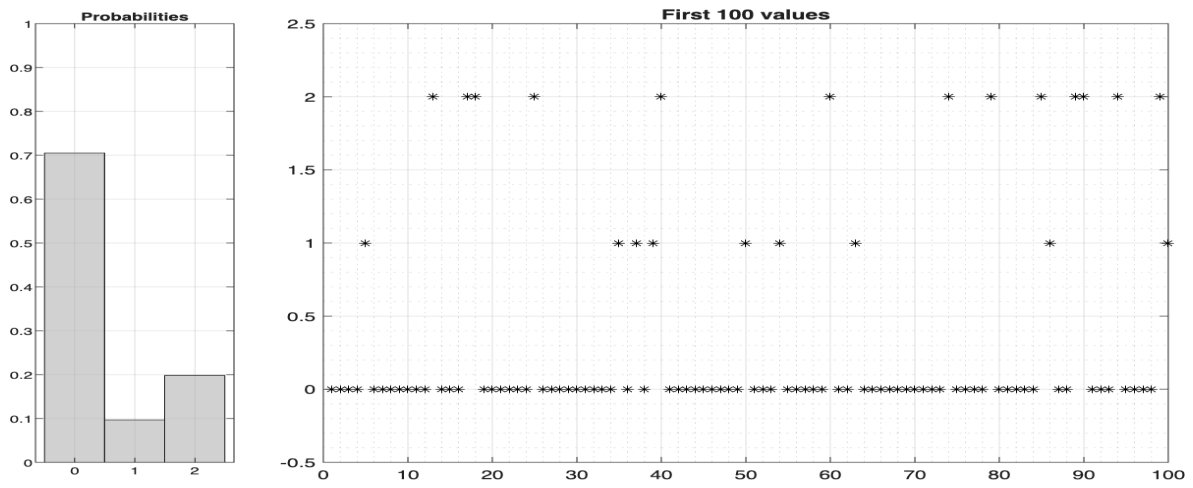
The results of the simulation using $N=10,000$ uniformly distributed points and $b=0.6$ are shown in Figure 2. The simulated expectation is close to (5):

$$\tilde{\mathbb{E}}\left(f\right)=0.7052·0+0.0967·1+0.1981·2=0.4929\approx \mathbb{E}\left(f\right).$$

The provided toolbox [32] allows simulations with different values of N, $a_0$, and $a_1$.

4. Example 3

The example provided in this section is preparation for the simulation of Feynman’s example in the next section.

At first sight, it looks similar to the example in Section 3 but does not allow obtaining the expressions for $g\left(x\right)$ and $h\left(x\right)$ in the form of polynomials. The key role here is played by the geometric probability distribution.

Let us consider a signed probability distribution f with the following probability-generating function:

$$f\left(x\right)=0.2+1.2x-0.4x^2.$$

(10)

The support of f is $\{0,1,2\}$, with $p_0=0.2$, $p_1=1.2$, and $p_2=-0.4$. Obviously, $p_0+p_1+p_2=1$, and

$$\mathbb{E}\left(f\right)=0.2·0+1.2·1+(-0.4)·2=0.4.$$

(11)

On the way to a generating function for $g\left(x\right)$, let us take some $0<q<1$, and consider

$$\tilde{g}\left(x\right)={\displaystyle \sum _{n=0}^{\infty }}{q}^n{x}^n$$

$$\tilde{h}\left(x\right)=f\left(x\right)\tilde{g}\left(x\right)=(0.2+1.2x-0.4x^2){\displaystyle \sum _{n=0}^{\infty }}{q}^n{x}^n.$$

Let $b_n$ be the coefficient of $x^n$ in $\tilde{h}\left(x\right)$. The first two coefficients are positive:

$$b_0=0.2>0,b_1=0.2q+1.2>0,$$

and we have to investigate the remaining coefficients $b_n$ for $n\ge 2$:

$$\begin{array}{ccc}\hfill b_n& =& 0.2q^n+1.2q^{n-1}-0.4q^{n-2}\hfill \\ & =& q^{n-2}\left(0.2q^2+1.2q-0.4\right).\hfill \end{array}$$

All $b_n>0$ for $n\ge 2$ if

$$0.2q^2+1.2q-0.4>0,$$

or

$$q^2+6q-2>0.$$

The roots are $r=-3\pm \sqrt{11}\approx -3\pm 3.3166$, and the root in $(0,1)$ is

$$r_{*}=-3+\sqrt{11}\approx 0.3166.$$

So, for

$$q\in (\sqrt{11}-3,1),$$

we get $\tilde{g}\left(x\right)$ with positive coefficients and $\tilde{h}\left(x\right)=\tilde{g}\left(x\right)f\left(x\right)$ also with all positive coefficients.

We need to ensure that the sum of the coefficients of g and h equals one. For the function $\tilde{g}\left(x\right)$ the sum of the coefficients is not one, but

$$S_q={\displaystyle \sum _{n=0}^{\infty }}{q}^n={\displaystyle \frac{1}{1-q}},$$

so we have to take $g\left(x\right)=(1-q)\tilde{g}\left(x\right)$, that is,

$$g\left(x\right)=(1-q){\displaystyle \sum _{n=0}^{\infty }}{q}^n{x}^n,$$

(12)

and then

$$h\left(x\right)=(1-q)f\left(x\right){\displaystyle \sum _{n=0}^{\infty }}{q}^n{x}^n.$$

(13)

Different values of $q\in (\sqrt{11}-3,1)$ yield different suitable pairs of ordinary non-negative probability distributions g and h given by their probability-generating functions (12) and (13), which can be used for simulations of the signed probability distribution f.

5. Example 4: Feynman’s Example

Now we can use the previous example (Section 4) for simulating the famous Feynman example of the idea of using negative probabilities [4]:

“First let us consider a simple probability problem, and how we usually calculate things, and then see what would happen if we allowed some of our normal probabilities in the calculations to be negative.”

The Feynman example can be presented as follows.

Suppose that a system can be in two conditions, A and B, occurring with probabilities $P\left(A\right)=0.7$ and $P\left(B\right)=0.3$, and in each of these conditions, the probabilities of the resulting outputs {0, 1, 2} are different (see

Table 1. Feynman’s example.

Result R	Condition A	Condition B
	P(A) = 0.7	P(B) = 0.3
$R_0=0$	0.1	0.2
$R_1=1$	0.6	1.2
$R_2=2$	0.3	$-0.4$

). Obviously,

$$P(R_0/A)+P(R_1/A)+P(R_2/A)=1,$$

$$P(R_0/B)+P(R_1/B)+P(R_2/B)=1,$$

and the total probabilities of the resulting outputs are

$$\begin{array}{ccc}& & P\left(R_0\right)=P(R_0/A)+P(R_0/B)=0.7·0.1+0.3·0.2=0.13,\hfill \\ & & P\left(R_1\right)=P(R_1/A)+P(R_1/B)=0.7·0.6+0.3·1.2=0.78,\hfill \\ & & P\left(R_2\right)=P(R_2/A)+P(R_2/B)=0.7·0.3+0.3·(-0.4)=0.09,\hfill \end{array}$$

and their sum is equal to one. The expectation $\mathbb{E}\left(R\right)$ of the system in the Feynman example is:

$$\mathbb{E}\left(R\right)=P\left(R_0\right)·R_0+P\left(R_1\right)·R_1+P\left(R_2\right)·R_2=0.96.$$

(14)

Feynman could not do numerical simulations due to the lack of tools for simulating signed probability distributions—but we can do that now.

For the simulation, let us generate, for example, $N=10,000$ uniformly distributed random points (the provided toolbox [32] allows simulations with different values of N).

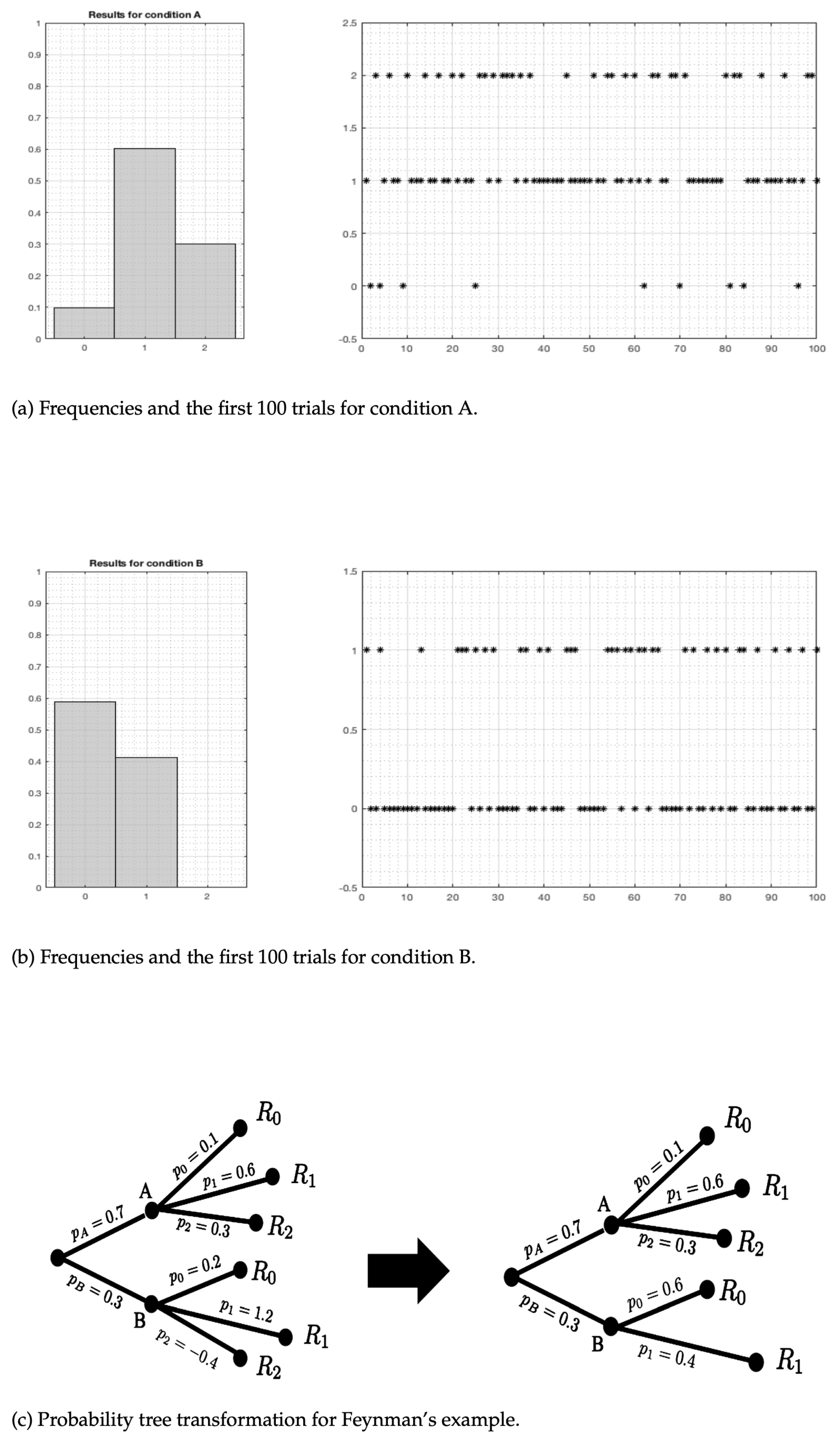
In the first stage of this particular numerical simulation, 6987 points fell to condition A, and 3013 points went to condition B.

In the second stage, the classical simulation for condition A produced 690 values of the output $R_0$, 4204 values of $R_1$, and 2093 values of $R_2$, which, in total, gives 6987 values that went to A. The frequencies of the output values and the first 100 trials are shown in Figure 3a.

The simulation for condition B realized following Section 4 with the parameter $q=0.9$ produced 1774 values of $R_0$, 1239 values of $R_1$, and zero values of $R_2$, which, in total, gives 3013 values that went to B. This means that the computed expectation for condition B is $0.5888·0+0.4112·1+0·2=0.4112$, which is close to what follows from (10). The frequencies of the output values and the first 100 trials are shown in Figure 3b.

Overall, the output $R_0$ appeared 2462 times, the output $R_1$ appeared 5263 times, and the output $R_2$ appeared 2093 times, giving the corresponding frequencies.

This means that the simulated expectation is close to (14):

$$\tilde{\mathbb{E}}\left(R\right)=0.2464R_0+0.5263R_1+0.2093R_2=0.9629\approx \mathbb{E}\left(R\right).$$

If we consider the signed probability tree representation of Table 1, shown in Figure 3c on the left, then we observe that it is actually equivalent to the probability tree with positive probabilities, which is shown on the right. Such understanding—reconfiguration of a probability tree with positive and negative probabilities into a probability tree with non-negative probabilities—applies also to other examples of the simulation of signed probability distributions provided in this paper. This opens wide possibilities for using signed probabilities in the fields of quantum computing, decision making, finance, insurance, large language models and artificial intelligence, and other fields where the use of signed probability distributions can extend the current level of mathematical modeling.

6. Extension of Feynman’s Example

Let us consider a slight generalization of Feynman’s example:

$$f\left(x\right)=a_0+a_{1}x-a_2{x}^2,$$

(15)

with $a_0>0$, $a_1>0$, $a_2>0$, $a_0+a_1+a_2=1$. Also, let us take $0<q<1$.

Let us take the same function $g\left(x\right)$ as in (12), then

$$h\left(x\right)=(1-q)\left(a_0+(a_1+a_{0}q)x+{\displaystyle \sum _{n=0}^{\infty }}\left(a_0{q}^2+a_{1}q-a_2\right)q^n{x}^{n+2}\right).$$

(16)

Figure 3. Feynman’s example.

Figure 3. Feynman’s example.

We are interested in having all coefficients of $h\left(x\right)$ positive. Having already $a_0>0$ and $a_1+a_{0}q>0$, we only have to require

$$a_0{q}^2+a_{1}q-a_2>0.$$

This allows us to produce more “Feynman-like” examples of probability-generating functions of signed probability distributions, for example, $f_1\left(x\right)=0.2+1.4x-0.6x^2$, $f_2\left(x\right)=0.5+0.6x-0.1x^2$, $f_3\left(x\right)=0.1+1.5x-0.6x^2$, etc.

7. Conclusions and Discussion

From Bartlett’s remark that “extraordinary random variables…can be defined only through their characteristic functions” it follows that we have to work with probability-generating functions. The Ruzsa–Székely theorem is the only currently available tool that guarantees the existence but not the uniqueness of a pair of two ordinary non-negative probability distributions, which can be used for simulating a signed (extended, generalized) probability distribution. Currently, there is no general method for finding such pairs of ordinary distributions for simulating a signed probability distribution. Finding a general method is an open problem of great importance.

The main characteristic, the expectation, is in simulations the same as the expectation computed formally using the output values of a random variable and the signed probabilities of those output values.

However, the results of simulations show that the computed frequencies of the output values differ from those signed probabilities, and these frequencies are naturally non-negative. Also, in some situations (see the examples in this paper and the paper [25]), the output values are also different from what one would expect from the signed probability-generating function.

The examples provided in this paper are the first ever of such kind, and they can be used as templates and benchmarks for other methods of simulation of signed probability distributions that might be developed in the future and/or as templates for creating other examples of simulations of signed probability distributions. Hopefully, they might be used for simulations in applied problems, where signed probability distributions of the considered types appear.

The presented method and examples of simulation might open wide possibilities for using signed probabilities in the fields of quantum computing, decision making, finance, insurance, large language models and artificial intelligence, and other fields where the use of negative probabilities and signed probability distributions can extend the current level of mathematical modeling.