Quadruple Controlled Metric-Type Spaces with Fixed-Point Results and Applications to Boundary Value Problem

Abstract

In this paper, we introduce a novel class of quadruple controlled metric-type spaces formulated in a four-dimensional setting. Within this framework, we extend the notion of a $\Theta$-contraction mapping to accommodate such spaces. By employing these concepts, we establish several new fixed-point theorems that significantly generalize and enhance the existing results in the literature. The validity and effectiveness of the proposed approach are demonstrated through carefully constructed illustrative examples within the defined space and for the derived fixed-point results. Finally, an application to a boundary value problem is presented, highlighting the potential of the developed theory. Furthermore, a coupled four-component thermo-chemical system was examined as an additional application, demonstrating the broader applicability of the proposed framework.

1. Introduction

Metric spaces constitute one of the most fundamental frameworks in analysis and fixed-point theory, providing the mathematical foundation for studying distance, convergence, continuity, and stability. Since their introduction, metric spaces have played a central role in establishing existence and uniqueness results for a wide variety of mathematical models [1]. However, the increasing complexity of modern applications has revealed limitations in the classical metric structure, particularly when interactions among several variables cannot be adequately represented through a conventional two-point distance.

To overcome these limitations, numerous generalizations of metric spaces have been developed over the years. These extensions aim to provide more flexible distance structures while preserving the essential properties required for fixed-point analysis. As a result, generalized metric frameworks have significantly broadened the scope of fixed-point theory and have enabled the study of nonlinear problems that cannot be effectively treated within classical metric spaces [2,3,4,5,6,7,8].

Among the most influential developments in this direction is the concept of an S-metric space introduced by Sedghi et al. [9], where the distance is determined by a function of three variables rather than two. This innovative approach stimulated extensive research activity and led to several important generalizations, including $S_b$-metric spaces [10], extended $S_b$-metric spaces [11], extended S-metric spaces of type $(\alpha ,\beta )$ [12], and triple controlled S-metric-type spaces [13], see also [14]. These generalized structures have provided increasingly flexible settings for establishing fixed-point theorems under weaker and more general contractive conditions.

Building on the development of two-variable and three-variable distance functions, Sarma et al. [15] introduced the concept of a four-dimensional metric space. This higher-dimensional framework allows the simultaneous treatment of interactions among four elements and provides a richer structure for modeling complex nonlinear phenomena. Such spaces are particularly useful when the generalized distance depends on several interrelated components whose collective behavior cannot be adequately represented within lower-dimensional settings.

From an application perspective, four-dimensional frameworks provide a natural setting for studying problems involving several interacting quantities simultaneously. In many mathematical models arising from differential equations, dynamical systems, coupled processes, and boundary value problems, the behavior of one component is often influenced by multiple related components. A four-dimensional distance structure enables these interactions to be incorporated directly into the underlying space rather than being treated separately. Consequently, it offers a more faithful representation of the intrinsic relationships among the variables and facilitates the formulation of contractive conditions that reflect the multi-component nature of the problem under consideration.

Although several advances have been achieved in four-dimensional metric spaces and their variants, the available frameworks remain relatively limited in terms of the flexibility of their control mechanisms. In particular, the existing approaches do not allow each component of the generalized distance to be governed independently. Consequently, certain classes of nonlinear mappings and contractive conditions cannot be naturally accommodated within the current four-dimensional setting. To the best of our knowledge, no quadruple controlled metric-type structure has yet been introduced in the context of four-dimensional metric spaces.

Motivated by these developments, we introduce a new class of spaces, termed quadruple controlled metric-type spaces (QCMSs)This framework generalizes controlled four-dimensional metric-type spaces through the incorporation of four independent control functions and may be regarded as a natural extension of the triple controlled metric-type spaces investigated in, among others [13,16], see also [5,6,8,13]. By assigning a distinct control function to each component of the generalized distance, the proposed structure offers a higher degree of flexibility and enables the treatment of a wider class of mappings and contractive conditions than those considered in existing four-dimensional settings.

The significance of QCMS extends beyond a straightforward increase in the number of control functions. The presence of an additional control parameter allows for a more refined representation of heterogeneous interactions among the four components of the generalized distance, making the framework particularly suitable for systems in which variables influence the underlying dynamics to different degrees. Such situations arise naturally in coupled boundary value problems and other nonlinear models involving multiple interacting states. Moreover, QCMS encompasses several known four-dimensional metric-type structures as special cases, thereby providing a unified and more general setting for the development of fixed-point theory and its applications.

The main contributions of this paper are summarized as follows. First, we introduce the notion of a quadruple controlled metric-type space and investigate its fundamental properties. Second, we extend the concept of a $\Theta$-contraction, originally introduced by Jleli and Samet [17], to this new framework and define the notion of a quadruple controlled ${\Theta }_{\Omega }$-contractive mapping. Third, we establish new existence and uniqueness theorems for fixed points in complete QCMSs, thereby extending and generalizing several related results available in the literature. Furthermore, illustrative examples are provided to demonstrate that the proposed framework genuinely extends existing four-dimensional metric-type structures. Finally, an application to a nonlinear boundary value problem is presented, illustrating the effectiveness of the developed theory and highlighting its potential for studying differential equations within generalized metric settings.

2. Preliminaries

The definition of the four-dimensional metric-type space was presented by Sarma et al. in [15].

Definition 1

([15]). Let $\Omega \ne \varnothing$, and let $B_4:{\Omega }^4\to [0,\infty )$ be a mapping so that for every $x,y,z,w$ and $a\in \Omega$, the following is satisfied:

(1) 

$B_4(x,y,z,w)=0$ iff $x=y=z=w$;

(2) 

$B_4(x,y,z,w)\le B_4(x,x,x,a)+B_4(y,y,y,a)+B_4(z,z,z,a)+B_4(w,w,w,a)$.

The pair $(\Omega ,B_4)$ is called a four-dimensional metric space.

We illustrate some examples of four-dimensional metric spaces.

Example 1

([15]). Let $\Omega \ne \varnothing$, and define the mapping $B_4:{\Omega }^4\to \mathbb{R}$, by

$$B_4(x,y,z,w)=\left\{\begin{array}{cc}0\hfill & \mathit{if}x=y=z=w,\hfill \\ 1\hfill & \mathit{otherwise}.\hfill \end{array}\right.$$

Then, $(\Omega ,B_4)$ is a four-dimensional metric space.

Example 2

([15]). Let $\Omega =\mathbb{R}$, and define the mapping $B_4:{\Omega }^4\to [0,\infty )$, for all $x,y,z,w\in \mathbb{R}$, by

$$B_4(x,y,z,w)=|x-z|+|y-z|+|x+y+z-3w|.$$

Then, $(\Omega ,B_4)$ is a four-dimensional metric space.

Example 3

([18]). Let $\Omega =\mathbb{N}\cup 0$, and define the mapping $B_4:{\Omega }^4\to [0,\infty )$ by

$$B_4(x,y,z,w)=\left\{\begin{array}{cc}0\hfill & \mathit{if}x=y=z=w,\hfill \\ x^2+y^2+z^2+w^2\hfill & \mathit{otherwise}.\hfill \end{array}\right.$$

Then, $(\Omega ,B_4)$ is a four-dimensional metric space.

The four-dimensional b-metric space is defined as an extension of a four-dimensional metric space. It relaxes the traditional triangle inequality by introducing a constant $s\ge 1$.

Definition 2.

Let $\Omega \ne \varnothing$ and let $\mathrm{{\rm Y}}:{\Omega }^4\to [0,\infty )$ be a mapping. Let $s\ge 1$ be a real constant; for every $x,y,z,w,a\in \Omega$, the following holds:

(1) 

$\mathrm{{\rm Y}}(x,y,z,w)=0$ if and only if $x=$ $y=z=w$;

(2) 

$\mathrm{{\rm Y}}(x,x,x,y)=\mathrm{{\rm Y}}(y,y,y,x)$;

(3) 

$\mathrm{{\rm Y}}(x,y,z,w)\le s\left[\mathrm{{\rm Y}}(x,x,x,a)+\mathrm{{\rm Y}}(y,y,y,a)+\mathrm{{\rm Y}}(z,z,z,a)+\mathrm{{\rm Y}}(w,w,w,a)\right].$

Then the pair $(\Omega ,\mathrm{{\rm Y}})$ is called a four-dimensional b-metric space.

The concept of a controlled four-dimensional metric-type space is defined below.

Definition 3.

Let $\Omega \ne \varnothing$, and let $\mathrm{{\rm Y}}:{\Omega }^4\to [0,\infty )$ be a mapping and consider the function $\mu :{\Omega }^2\to [1,\infty )$, so that for every $x,y,z,w$ and $a\in \Omega$, the following is satisfied:

(1) 

$\mathrm{{\rm Y}}(x,y,z,w)=0$ if $x=y=z=w$;

(2) 

$\mathrm{{\rm Y}}(x,x,x,y)=\mathrm{{\rm Y}}(y,y,y,x)$;

(3) 

$\mathrm{{\rm Y}}(x,y,z,w)\le \mu (x,a)\mathrm{{\rm Y}}(x,x,x,,a)+\mu (y,a)\mathrm{{\rm Y}}(y,y,y,a)+\mu (z,a)\mathrm{{\rm Y}}(z,z,z,a)+\mu (w,a)\mathrm{{\rm Y}}(w,w,w,a)$.

The pair $(\Omega ,\mathrm{{\rm Y}})$ is called a controlled four-dimensional metric-type space.

Next, we introduce the novel concept of a quadruple controlled four-dimensional metric-type space, which serves as a natural generalization of the triple controlled metric-type space; see, for example, [13,16]. The introduction of a fourth control function significantly enhances the flexibility of the underlying distance structure, allowing for a more refined characterization of interactions among multiple variables.

Definition 4.

Let $\Omega \ne \varnothing$, and let $\mathrm{{\rm Y}}:{\Omega }^4\to [0,\infty )$ be a mapping and consider the control functions $\beta ,\mu ,\gamma ,\eta :{\Omega }^2\to [1,\infty )$, such that for all $x,y,z,w$ and $a\in \Omega$, it satisfies the following:

(1) 

$\mathrm{{\rm Y}}(x,y,z,w)=0$ iff $x=y=z=w$;

(2) 

$\mathrm{{\rm Y}}(x,x,x,y)=\mathrm{{\rm Y}}(y,y,y,x)$.

(3) 

$\mathrm{{\rm Y}}(x,y,z,w)\le \beta (x,a)\mathrm{{\rm Y}}(x,x,x,,a)+\mu (y,a)\mathrm{{\rm Y}}(y,y,y,a)+\eta (z,a)\mathrm{{\rm Y}}(z,z,z,a)+\gamma (w,a)\mathrm{{\rm Y}}(w,w,w,a)$.

The pair $(\Omega ,\mathrm{{\rm Y}})$ is called a quadruple controlled metric-type space; it will be abbreviated by $QCMS$.

Remark 1.

For special cases, Definition 4 yields the following concepts:

(1) 

By taking

$$\beta (x,a)=\mu (x,a)=\gamma (x,a)=\eta (x,a),for allx,a\in \Omega ,$$

in Definition 4, the pair $(\Omega ,\mathrm{{\rm Y}})$ reduces to a controlled four-dimensional metric space.

(2) 

By taking

$$\beta (x,a)=\mu (x,a)=\gamma (x,a)=\eta (x,a)=s\ge 1,for allx,a\in \Omega ,$$

in Definition 4, then $(\Omega ,\mathrm{{\rm Y}})$ reduces to a four-dimensional b-metric space.

(3) 

By taking $s=1$, in Definition 4, then $(\Omega ,\mathrm{{\rm Y}})$ reduces to a four-dimensional metric space.

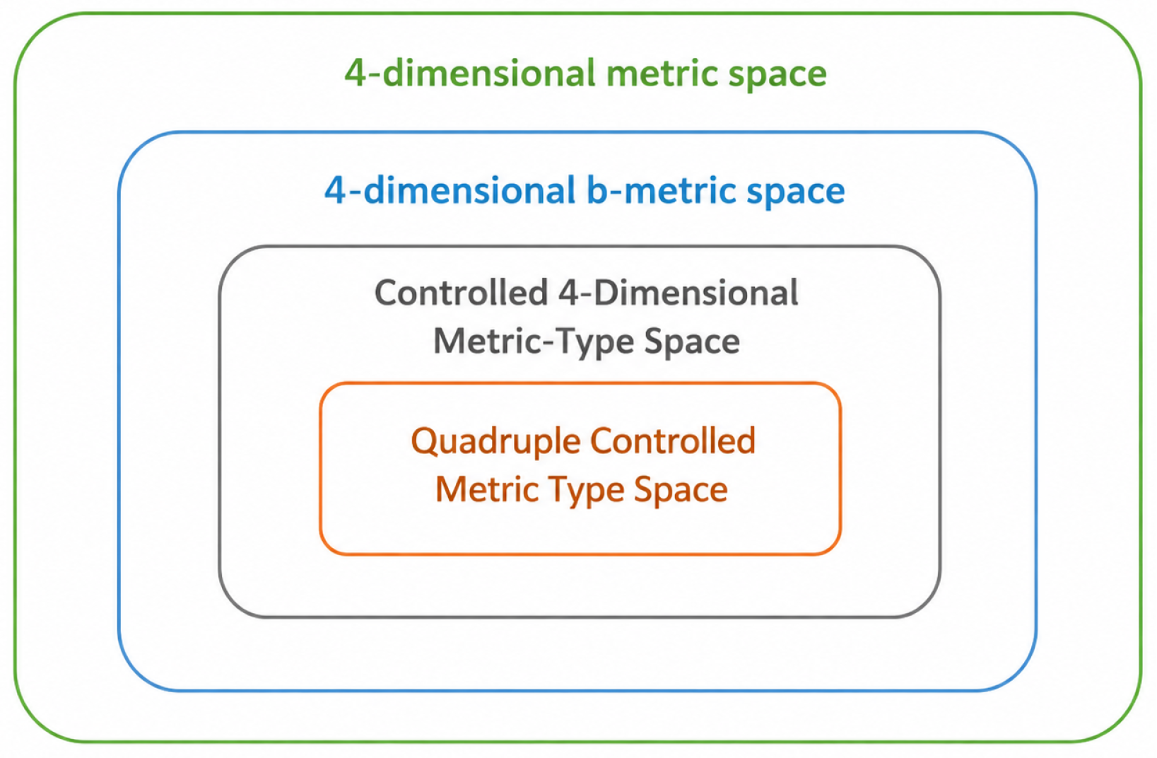
The preceding remark yields the following inclusion relationship:

Quadruple controlled metric-type space ⊂ controlled four-dimensional metric-type space ⊂ four-dimensional b-metric-type space ⊂ four-dimensional metric-type space.

A schematic representation of these inclusions is provided in Figure 1.

Examples of quadruple controlled metric-type spaces are presented below.

Example 4.

Let $\Omega =\{1,2,3,4\}$, and define the mapping $\mathrm{{\rm Y}}:{\Omega }^4\to [0,\infty )$ and the control functions $\beta ,\mu ,\eta ,\gamma :{\Omega }^2\to [1,\infty )$ by:

$$\mathrm{{\rm Y}}(x,y,z,w)=\left\{\begin{array}{cc}0\hfill & \mathit{if}x=y=z=w,\hfill \\ {\displaystyle \frac{1}{x}}\hfill & \mathit{if}x=y=z\mathit{is}\mathit{even},\mathit{and}w\mathit{is}\mathit{odd}\hfill \\ {\displaystyle \frac{1}{w}}\hfill & \mathit{if}w\mathit{is}\mathit{even},\mathit{and}x=y=z\mathit{is}\mathit{odd}\hfill \\ 1\hfill & \mathit{otherwise}.\hfill \end{array}\right.$$

and, $\beta (x,a)=1+x+a,\mu (x,a)=1+xa,\eta (x,a)=1,$ and $\gamma (x,a)=2+x+a$.

One can easily show that condition (1) of Definition 4 is satisfied. To show condition (2) is satisfied, we need to consider cases; for example, if $x=y=z$ is even and w is odd, then

$$\mathrm{{\rm Y}}(x,x,x,y)={\displaystyle \frac{1}{x}}=\mathrm{{\rm Y}}(y,y,y,x).$$

Similarly for the other cases. To verify condition (3), let us take, for example, $x=1,y=2,z=3,w=4$ and suppose $a=2$, we see that

$$\begin{array}{ccc}\hfill \mathrm{{\rm Y}}(1,2,3,4)=1& \le & \beta (1,2)\mathrm{{\rm Y}}(1,1,1,2)+\mu (2,2)\mathrm{{\rm Y}}(2,2,2,2)\hfill \\ & & +\eta (3,2)\mathrm{{\rm Y}}(3,3,3,2)+\gamma (4,2)\mathrm{{\rm Y}}(4,4,4,2).\hfill \\ & \le & (1+2+1)(1/2)+(1+4)\left(0\right)+1(1/2)+(2+4+2)\left(1\right).\hfill \\ & =& 2+0+1/2+8=21/2.\hfill \end{array}$$

Next, if $x=y=z=2,w=4$ and suppose $a=3$, we see that

$$\begin{array}{ccc}\hfill \mathrm{{\rm Y}}(2,2,2,4)={\displaystyle \frac{1}{2}}& \le & \beta (2,3)\mathrm{{\rm Y}}(2,2,2,3)+\mu (2,3)\mathrm{{\rm Y}}(2,2,2,3)\hfill \\ & & +\eta (2,3)\mathrm{{\rm Y}}(2,2,2,3)+\gamma (4,3)\mathrm{{\rm Y}}(3,3,3,4).\hfill \\ & \le & (1+2+3)(1/2)+(1+2(3\left)\right)(1/2)+1(1/2)+(2+3+4)(1/4).\hfill \\ & =& 6/2+7/2+1/2+9/4=37/4.\hfill \end{array}$$

In similar way, one can check all the other cases; hence, $(\Omega ,\mathrm{{\rm Y}})$ is a quadruple controlled metric space. Note that as $\beta \ne \mu \ne \eta \ne \gamma$; hence, this is an example of a quadruple controlled metric-type space which is not a controlled four-dimensional metric-type space. Furthermore, clearly it is not a four-dimensional b-metric-type space.

Example 5.

Let $\Omega =[0,2]$. Define the mapping $\mathrm{{\rm Y}}:{\Omega }^4\to [0,\infty )$ by $\mathrm{{\rm Y}}(x,y,z,w)=|x-z|+|y-z|+|x+y+z-3w|$. Consider the functions $\beta ,\mu ,\eta ,\gamma :\Omega \times \Omega \to [1,\infty )$ defined by $\beta (x,y)=1+x+y$, $\mu (x,y)=1+x$, $\eta (x,y)=1+y$, and

$$\gamma (x,y)=\left\{\begin{array}{cc}x+y\hfill & \mathit{if}x\in [0,1),\hfill \\ 1\hfill & \mathit{otherwise}.\hfill \end{array}\right.$$

One can verify that $(\Omega ,\mathrm{{\rm Y}})$ is a quadruple controlled metric-type space.

Next, we recall the notions of convergent and Cauchy sequences, along with completeness and open balls in a $QCMS$.

Definition 5.

Let $(\Omega ,\mathrm{{\rm Y}})$ be a $QCMS$ and let $\left\{x_n\right\}$ be any sequence in Ω.

(1) We say the sequence $\left\{x_n\right\}$ converges to w in $\Omega ,$ if $\mathrm{{\rm Y}}(x_n,x_n,x_n,w)\to 0$, as $n\to \infty$. Furthermore, from the symmetry, this also gives $\mathrm{{\rm Y}}(w,w,w,x_n)\to 0$, as $n\to \infty$.

(2) The sequence $\left\{x_n\right\}$ is referred to as a Cauchy sequence if for every $\epsilon >0$, there exists $N\in \mathbb{N}$ such that $\mathrm{{\rm Y}}(x_n,x_n,x_n,x_m)<\epsilon$ for all $m,n\ge N.$

(3) The space $(\Omega ,\mathrm{{\rm Y}})$ is called complete if every Cauchy sequence in Ω is convergent.

The next lemma illustrates the uniqueness of the limit of a convergent sequence.

Lemma 1.

Let $(\Omega ,\mathrm{{\rm Y}})$ be a $QCMS$ and let $\left\{x_n\right\}$ be any sequence in Ω. Furthermore, the limits of the control functions $\beta ,\mu ,\gamma ,\eta :{\Omega }^2\to [1,\infty )$ exists. If the sequence is convergent then its limits is unique.

Proof. 

$$\begin{array}{ccc}\hfill \mathrm{{\rm Y}}(x,x,x,y)& \le & \beta (x,x_n)\mathrm{{\rm Y}}(x,x,x,x_n)+\mu (x,x_n)\mathrm{{\rm Y}}(x,x,x,x_n)\hfill \\ & +& \eta (x,x_n)\mathrm{{\rm Y}}(x,x,x,x_n)+\gamma (y,x_n)\mathrm{{\rm Y}}(y,y,y,x_n).\hfill \end{array}$$

(1)

Taking the limit as n tends to infinity in Equation (1), and the fact ${lim}_{n\to \infty }\beta (x,x_n),$${lim}_{n\to \infty }\mu (x,x_n)$, ${lim}_{n\to \infty }\eta (x,x_n)$ and ${lim}_{n\to \infty }\gamma (x,x_n),$ exists and is finite. We conclude $\mathrm{{\rm Y}}(x,x,x,y)=0,$ and thus, $x=y$. □

Jleli and Samet [17] introduced a new type of contraction which is called the $\Theta$-contraction and established some new fixed-point theorems for such a contraction in the context of generalized metric spaces.

Definition 6.

Let Θ denote the collection of all mappings $\theta :(0,\infty )\to (1,\infty )$ that satisfy the following properties:

(θ1) θ is non-decreasing.

(θ2) For every sequence $\left\{t_m\right\}\subset (0,\infty )$,

$$\underset{m\to \infty }{lim}{t}_m=0^{+}\iff \underset{m\to \infty }{lim}\theta \left(t_m\right)=1.$$

(θ3) There exist constants $k\in (0,1)$, and $M\in (0,\infty ]$, such that

$$\underset{t\to 0^{+}}{lim}{\displaystyle \frac{\theta \left(t\right)-1}{t^k}}=M.$$

The notion of a $\Theta$-contraction within the framework of a quadruple controlled metric-type space $(\Omega ,\mathrm{{\rm Y}})$ will be referred to as a ${\Theta }_{\Omega }$-contraction. Next, we present the definition of quadruple controlled ${\Theta }_{\Omega }$-contractive mapping.

Definition 7.

Consider a quadruple controlled metric-type space $(\Omega ,\mathrm{{\rm Y}})$ with Ω non-empty, and let $T:\Omega \to \Omega$ be a mapping. Then, T is called a quadruple controlled ${\Theta }_{\Omega }$-contractive mapping provided that there exist $\theta \in {\Theta }_{\Omega }$ and a constant $r\in (0,1)$ for which the following condition is fulfilled:

$$\begin{array}{ccc}\hfill \mathit{For}\mathit{all}x,y,z,w\in \Omega ,& with& \mathrm{{\rm Y}}(Tx,Ty,Tz,Tw)\ne 0,then\hfill \\ & & \theta \left(\mathrm{{\rm Y}}(Tx,Ty,Tz,Tw)\right)\le {\left[\theta \left(\mathrm{{\rm Y}}(x,y,z,w)\right)\right]}^r.\hfill \end{array}$$

3. Main Results

In this section, we present two main fixed-point theorems in the setting of a complete quadruple controlled metric-type Space $(\Omega ,\mathrm{{\rm Y}})$. The first theorem is established using the concept of a quadruple controlled ${\Theta }_{\Omega }$–contractive mapping, while the second result is obtained through another contractive condition adapted to the QCMS framework. By combining these contractive assumptions with the structural inequality given in Definition 4, we construct a Picard iterative sequence and prove that it is Cauchy. The completeness of the space ensures the convergence of the sequence, leading to the existence and uniqueness of the fixed point for the considered mappings.

Theorem 1.

Let $(\Omega ,\mathrm{{\rm Y}})$ be a complete $QCMS$, where $\Omega \ne \varnothing$. Let $T:\Omega \to \Omega$ be a quadruple controlled ${\Theta }_{\Omega }$-contraction, as in Definition 7. For any $x_0\in \Omega$, the sequence $\left\{x_n\right\}$ is formed by $x_n=T^n{x}_0$; assume that the following holds:

$$\underset{m\ge 1}{sup}\underset{n\to \infty }{lim}{\displaystyle \frac{\gamma (x_m,x_{n+1})\left[\beta (x_{n+1},x_{n+2})+\mu (x_{n+1},x_{n+2})+\eta (x_{n+1},x_{n+2})\right]}{[\beta (x_n,x_{n+1})+\mu (x_n,x_{n+1})+\eta (x_n,x_{n+1})]}}<1.$$

(2)

In addition, for each $x\in \Omega$, the limits

$$\underset{n\to \infty }{lim}\beta (x,x_n),\underset{n\to \infty }{lim}\mu (x_n,x),\underset{n\to \infty }{lim}\eta (x_n,x),\underset{n\to \infty }{lim}\gamma (x_n,x)$$

(3)

and

$$\underset{n\to \infty }{lim}\beta (x_n,x),\underset{n\to \infty }{lim}\mu (x,x_n),\underset{n\to \infty }{lim}\eta (x,x_n)\mathrm{and}\underset{n\to \infty }{lim}\gamma (x,x_n)\mathrm{exists}\mathrm{and}\mathrm{finite}.$$

(4)

Then, T possesses a unique fixed point in Ω.

Proof. 

Let $x_0$ be any arbitrary point in $\Omega$. Construct a sequence $\left\{x_n\right\}$ using an iteration as follows: $T{x}_0=x_1,T{x}_1=x_2$; thus, $T^n{x}_0=x_n,$ for all $n\in N$.

If for some $m\in \mathbb{N}$, $T^m{x}_0=T^{m+1}{x}_0$, then this implies that $T^m{x}_0$ is a fixed point of the mapping T. Hence, without loss of generality, we can suppose that $x_n\ne x_{n+1}$, i.e.,

$$\mathrm{{\rm Y}}(T^n{x}_0,T^n{x}_0,T^n{x}_0,T^{n+1}{x}_0)>0,\mathrm{for}\mathrm{all}n\in \mathbb{N}.$$

Utilizing 2 and applying it recursively, we obtain

$$\begin{array}{cc}\hfill \theta \left(\mathrm{{\rm Y}}(x_n,x_n,x_n,x_{n+1})\right)& =\theta \left(\mathrm{{\rm Y}}(T{x}_{n-1},T{x}_{n-1},T{x}_{n-1},T{x}_n)\right)\hfill \\ & \le {\left[\theta \left(\mathrm{{\rm Y}}(x_{n-1},x_{n-1},x_{n-1},x_n)\right)\right]}^r\hfill \\ & \le {\left[\theta \left(\mathrm{{\rm Y}}(x_{n-2},x_{n-2},x_{n-2},x_{n-1})\right)\right]}^{r^2}\hfill \\ & \le {\left[\theta \left(\mathrm{{\rm Y}}(x_{n-3},x_{n-3},x_{n-3},x_{n-2})\right)\right]}^{r^3}\le \cdots \le {\left[\theta \left(\mathrm{{\rm Y}}(x_0,x_0,x_0,x_1)\right)\right]}^{r^n}\hfill \end{array}$$

(5)

Therefore, as $\theta \left(t\right)>1$, we have

$$1<\theta \left(\mathrm{{\rm Y}}(x_n,x_n,x_n,x_{n+1})\right)\le {\left[\theta \left(\mathrm{{\rm Y}}(x_0,x_0,x_0,x_1)\right)\right]}^{r^n}.$$

(6)

As $0<r<1$, by making n tends to infinity in Equation (6), we deduce

$$\underset{n\to \infty }{lim}\theta \left(\mathrm{{\rm Y}}(x_n,x_n,x_n,x_{n+1})\right)=1.$$

Employing property $\left(\theta 2\right)$, we obtain

$$\underset{n\to \infty }{lim}\mathrm{{\rm Y}}(x_n,x_n,x_n,x_{n+1})=0.$$

(7)

By $\left(\theta 3\right)$, there exists k such that $0<k<1$ and $M\in (0,\infty ]$ so that

$$\underset{n\to \infty }{lim}{\displaystyle \frac{\theta \left(\mathrm{{\rm Y}}(x_n,x_n,x_n,x_{n+1})\right)-1}{{\left[\mathrm{{\rm Y}}(x_n,x_n,x_n,x_{n+1})\right]}^k}}=M.$$

(8)

Case 1: Assume $0<M<\infty$, and let $L={\displaystyle \frac{M}{2}}$; by Equation (8), there is some $n_0\in N$, such that for all $n\ge n_0$, we obtain

$$\left|{\displaystyle \frac{\theta \left(\mathrm{{\rm Y}}(x_n,x_n,x_n,x_{n+1})\right)-1}{{\left[\mathrm{{\rm Y}}(x_n,x_n,x_n,x_{n+1})\right]}^k}}-M\right|\le L.$$

This yields

$$L=M-L\le {\displaystyle \frac{\theta \left(\mathrm{{\rm Y}}(z_n,z_{n+1})\right)-1}{{\left[\mathrm{{\rm Y}}(z_n,z_{n+1})\right]}^k}},\forall n\ge n_0.$$

Thus, for every $n\ge n_0$, we have

$$n{\left[\mathrm{{\rm Y}}(x_n,x_n,x_n,x_{n+1})\right]}^k\le n[{\displaystyle \frac{\theta \left(\mathrm{{\rm Y}}(x_n,x_n,x_n,x_{n+1})\right)-1}{L}}]$$

By utilizing (6), we get

$$n{\left[\mathrm{{\rm Y}}(x_n,x_n,x_n,x_{n+1})\right]}^k\le n[{\displaystyle \frac{{\left[\theta \left(\mathrm{{\rm Y}}(x_0,x_0,x_0,x_1)\right)\right]}^{r^n}-1}{L}}].$$

As $n\to \infty$, in the above inequality, we obtain

$$\underset{n\to \infty }{lim}n[\mathrm{{\rm Y}}{\left((x_n,x_n,x_n,x_{n+1})\right]}^k=0.$$

(9)

Case 2: Let $M=\infty$; assume that $L>0$ is arbitrary. Then, by the definition of the limit, there exists $n_1\in N$ such that

$${\displaystyle \frac{\theta \left(\mathrm{{\rm Y}}(x_n,x_n,x_n,x_{n+1})\right)-1}{{\left[\mathrm{{\rm Y}}(x_n,x_n,x_n,x_{n+1})\right]}^k}}\ge L,\forall n\ge n_1,$$

which gives

$$n{\left[\mathrm{{\rm Y}}(x_n,x_n,x_n,x_{n+1})\right]}^k\le n[{\displaystyle \frac{\theta \left(\mathrm{{\rm Y}}(x_n,x_n,x_n,x_{n+1})\right)-1}{L}}]$$

Again, utilizing (6) in the above inequality and then making $n\to \infty$, we get

$$\underset{n\to \infty }{lim}n{\left[\mathrm{{\rm Y}}(x_n,x_n,x_n,x_{n+1})\right]}^k=0.$$

(10)

Thus, combining (9) and (10), we conclude that for any $M\in (0,\infty ]$ and $0<k<1,$ there exists some $\widehat{N}\in N$, where $\tilde{N}=max\{n_0,n_1\}$ such that

$$\mathrm{{\rm Y}}(x_n,x_n,x_n,x_{n+1})\le {\displaystyle \frac{1}{n^{1/k}}},\forall n\ge \widehat{N}.$$

(11)

To demonstrate $\left\{x_n\right\}$ is a Cauchy sequence, consider all $m,n\in \mathbb{N}$ with condition $n<m$; thus, we obtain;

$$\begin{array}{cc}\hfill \mathrm{{\rm Y}}(x_n,x_n,x_n,x_m)& \le \beta (x_n,x_{n+1})\mathrm{{\rm Y}}(x_n,x_n,x_n,x_{n+1})+\mu (x_n,x_{n+1})\mathrm{{\rm Y}}(x_n,x_n,x_n,x_{n+1})\hfill \\ & +\eta (x_n,x_{n+1})\mathrm{{\rm Y}}(x_n,x_n,x_n,x_{n+1})+\gamma (x_m,x_{n+1})\mathrm{{\rm Y}}(x_{n+1},x_{n+1},x_{n+1},x_m).\hfill \\ & \le \beta (x_n,x_{n+1})\mathrm{{\rm Y}}(x_n,x_n,x_n,x_{n+1})+\mu (x_n,x_{n+1})\mathrm{{\rm Y}}(x_n,x_n,x_n,x_{n+1})\hfill \\ & +\eta (x_n,x_{n+1})\mathrm{{\rm Y}}(x_n,x_n,x_n,x_{n+1})\hfill \\ & +\gamma (x_m,x_{n+1})[\beta (x_{n+1},x_{n+2})\mathrm{{\rm Y}}(x_{n+1},x_{n+1},x_{n+1},x_{n+2})\hfill \\ & +\mu (x_{n+1},x_{n+2})\mathrm{{\rm Y}}(x_{n+1},x_{n+1},x_{n+1},x_{n+2})+\eta (x_{n+1},x_{n+2})\mathrm{{\rm Y}}(x_{n+1},x_{n+1},x_{n+1},x_{n+2})\hfill \\ & +\gamma (x_m,x_{n+2})\mathrm{{\rm Y}}(x_{n+2},x_{n+2},x_{n+2},x_m)].\hfill \\ & \le \beta (x_n,x_{n+1})\mathrm{{\rm Y}}(x_n,x_n,x_n,x_{n+1})+\mu (x_n,x_{n+1})\mathrm{{\rm Y}}(x_n,x_n,x_n,x_{n+1})\hfill \\ & +\eta (x_n,x_{n+1})\mathrm{{\rm Y}}(x_n,x_n,x_n,x_{n+1})\hfill \\ & +\gamma (x_m,x_{n+1})\beta (x_{n+1},x_{n+2})\mathrm{{\rm Y}}(x_{n+1},x_{n+1},x_{n+1},x_{n+2})\hfill \\ & +\gamma (x_m,x_{n+1})\mu (x_{n+1},x_{n+2})\mathrm{{\rm Y}}(x_{n+1},x_{n+1},x_{n+1},x_{n+2})\hfill \\ & +\gamma (x_m,x_{n+1})\eta (x_{n+1},x_{n+2})\mathrm{{\rm Y}}(x_{n+1},x_{n+1},x_{n+1},x_{n+2})\hfill \\ & +\gamma (x_m,x_{n+1})\gamma (x_m,x_{n+2})[\beta (x_{n+2},x_{n+3})\mathrm{{\rm Y}}(x_{n+2},x_{n+2},x_{n+2},x_{n+3})\hfill \\ & +\mu (x_{n+2},x_{n+3})\mathrm{{\rm Y}}(x_{n+2},x_{n+2},x_{n+2},x_{n+3})\hfill \\ & +\eta (x_{n+2},x_{n+3})\mathrm{{\rm Y}}(x_{n+2},x_{n+2},x_{n+2},x_{n+3})\hfill \\ & +\gamma (x_m,x_{n+3})\mathrm{{\rm Y}}(x_{n+3},x_{n+3},x_{n+3},x_m)].\hfill \\ \hfill ⋮& \end{array}$$

$$\begin{array}{cc}\hfill \mathrm{{\rm Y}}(x_n,x_n,x_n,x_m)& \le \beta (x_n,x_{n+1})\mathrm{{\rm Y}}(x_n,x_n,x_n,x_{n+1})+\mu (x_n,x_{n+1})\mathrm{{\rm Y}}(x_n,x_n,x_n,x_{n+1})\hfill \\ & +\eta (x_n,x_{n+1})\mathrm{{\rm Y}}(x_n,x_n,x_n,x_{n+1})\hfill \\ & +{\displaystyle \sum _{i=n+1}^{m-2}}[\beta (x_i,x_{i+1})+\mu (x_i,x_{i+1})+\eta (x_i,x_{i+1})]\mathrm{{\rm Y}}(x_i,x_i,x_i,x_{i+1})\left({\displaystyle \prod _{j=n+1}^i}\gamma (x_m,x_j)\right)\hfill \\ & +{\displaystyle \prod _{i=n+1}^{m-1}}\gamma (x_m,x_i)\mathrm{{\rm Y}}(x_{m-1},x_{m-1},x_{m-1},x_m).\hfill \end{array}$$

$$\begin{array}{cc}\hfill \mathrm{{\rm Y}}(x_n,x_n,x_n,x_m)& \le [\beta (x_n,x_{n+1})+\mu (x_n,x_{n+1})+\eta (x_n,x_{n+1})]\mathrm{{\rm Y}}(x_n,x_n,x_n,x_{n+1})\hfill \\ & +{\displaystyle \sum _{i=n+1}^{m-1}}[\beta (x_i,x_{i+1})+\mu (x_i,x_{i+1})+\eta (x_i,x_{i+1})]\mathrm{{\rm Y}}(x_i,x_i,x_i,x_{i+1})\left({\displaystyle \prod _{j=n+1}^i}\gamma (x_m,x_j)\right)\hfill \end{array}$$

(12)

Applying Equation (11) into Equation (12), it becomes

$$\begin{array}{cc}\hfill \mathrm{{\rm Y}}(x_n,x_n,x_n,x_m)& \le [\beta (x_n,x_{n+1})+\mu (x_n,x_{n+1})+\eta (x_n,x_{n+1})]({\displaystyle \frac{1}{n^{1/k}}})\hfill \\ & +{\displaystyle \sum _{i=n+1}^{m-1}}[\beta (x_i,x_{i+1})+\mu (x_i,x_{i+1})+\eta (x_i,x_{i+1})]({\displaystyle \frac{1}{i^{1/k}}})\left({\displaystyle \prod _{j=n+1}^i}\gamma (x_m,x_j)\right)\hfill \\ & \le [\beta (x_n,x_{n+1})+\mu (x_n,x_{n+1})+\eta (x_n,x_{n+1})]({\displaystyle \frac{1}{n^{1/k}}})\hfill \\ & +{\displaystyle \sum _{i=1}^{m-1}}[\beta (x_i,x_{i+1})+\mu (x_i,x_{i+1})+\eta (x_i,x_{i+1})]({\displaystyle \frac{1}{i^{1/k}}})\left({\displaystyle \prod _{j=1}^i}\gamma (x_m,x_j)\right).\hfill \end{array}$$

(13)

$$\begin{array}{cc}\hfill \mathrm{{\rm Y}}(x_n,x_n,x_n,x_m)& \le [\beta (x_n,x_{n+1})+\mu (x_n,x_{n+1})+\eta (x_n,x_{n+1})]\left({\displaystyle \frac{1}{n^{1/k}}}\right)\hfill \\ & +{\displaystyle \sum _{i=1}^{\infty }}[\beta (x_i,x_{i+1})+\mu (x_i,x_{i+1})+\eta (x_i,x_{i+1})]\left({\displaystyle \frac{1}{i^{1/k}}}\right)\left({\displaystyle \prod _{j=1}^i}\gamma (x_m,x_j)\right).\hfill \end{array}$$

First note that by (4), it follows that

$$\underset{n\to \infty }{lim}[\beta (x_n,x_{n+1})+\mu (x_n,x_{n+1})+\eta (x_n,x_{n+1})]\left({\displaystyle \frac{1}{n^{1/k}}}\right)=0.$$

(14)

Next, we show the series in (14) is absolutely convergent using the ratio test.

Let

$$a_i=\left[\beta (x_i,x_{i+1})+\mu (x_i,x_{i+1})+\eta (x_i,x_{i+1})\right]\left({\displaystyle \frac{1}{i^{1/k}}}\right)\left({\displaystyle \prod _{j=1}^i}\gamma (x_m,x_j)\right),i\ge 1.$$

Observe that

$${\displaystyle \frac{a_{i+1}}{a_i}}={\displaystyle \frac{[\beta (x_{i+1},x_{i+2})+\mu (x_{i+1},x_{i+2})+\eta (x_{i+1},x_{i+2})]\left(\frac{1}{{(i+1)}^{1/k}}\right)\left({\prod }_{j=1}^{i+1}\gamma (x_m,x_j)\right)}{\left[\beta (x_i,x_{i+1})+\mu (x_i,x_{i+1})+\eta (x_i,x_{i+1})\right]\left(\frac{1}{i^{1/k}}\right)\left({\prod }_{j=1}^i\gamma (x_m,x_j)\right)}}.$$

Hence,

$${\displaystyle \frac{a_{i+1}}{a_i}}={\displaystyle \frac{\gamma (x_m,x_{i+1})\left[\beta (x_{i+1},x_{i+2})+\mu (x_{i+1},x_{i+2})+\eta (x_{i+1},x_{i+2})\right]}{\left[\beta (x_i,x_{i+1})+\mu (x_i,x_{i+1})+\eta (x_i,x_{i+1})\right]}}{\left({\displaystyle \frac{i}{i+1}}\right)}^{1/k}.$$

Taking the limit as $i\to \infty$, and using assumption (2), together with

$$\underset{i\to \infty }{lim}{\left({\displaystyle \frac{i}{i+1}}\right)}^{1/k}=1,$$

Apply the ratio test

$$\underset{i\to \infty }{lim}{\displaystyle \frac{a_{i+1}}{a_i}}=\underset{m\ge 1}{sup}\underset{i\to \infty }{lim}{\displaystyle \frac{\gamma (x_m,x_{i+1})\left[\beta (x_{i+1},x_{i+2})+\mu (x_{i+1},x_{i+2})+\eta (x_{i+1},x_{i+2})\right]}{\left[\beta (x_i,x_{i+1})+\mu (x_i,x_{i+1})+\eta (x_i,x_{i+1})\right]}}<1.$$

(15)

Therefore, by Equations (14) and (15), we deduce

$$\underset{n,m\to \infty }{lim}\mathrm{{\rm Y}}(x_n,x_n,x_n,x_m)=0.$$

We conclude that $\left\{x_n\right\}$ is a Cauchy sequence. From the completeness of $(\Omega ,\mathrm{{\rm Y}})$, the sequence converges to some $u\in \Omega$, i.e.,

$$\underset{n\to \infty }{lim}\mathrm{{\rm Y}}(x_n,x_n,x_n,u)=0.$$

(16)

In the following paragraph, we will illustrate that $u$ is a fixed point of the mapping $T$, i.e., $Tu=u$. Initially, we will show that ${lim}_{n\to \infty }\mathrm{{\rm Y}}(T{x}_n,T{x}_n,T{x}_n,Tu)=0.$

Assume that $\mathrm{{\rm Y}}(T{x}_n,T{x}_n,T{x}_n,Tu)>0$ for all n. By Definition 6, we have

$$ln\left(\theta \left(\mathrm{{\rm Y}}(T{x}_n,T{x}_n,T{x}_n,Tu)\right)\right)\le r\left(ln\left(\theta \left(\mathrm{{\rm Y}}(x_n,x_n,x_n,u)\right)\right)\right)\le ln\left(\theta \left(\mathrm{{\rm Y}}(x_n,x_n,x_n,u)\right)\right),$$

which implies by $\left(\theta 1\right)$ that $\mathrm{{\rm Y}}(T{x}_n,T{x}_n,T{x}_n,Tu)\le \mathrm{{\rm Y}}(x_n,x_n,x_n,u)$. Taking the limit as n tends to infinity, this gives ${lim}_{n\to \infty }\mathrm{{\rm Y}}(T{x}_n,T{x}_n,T{x}_n,Tu)=0$. Therefore, from

$$\mathrm{{\rm Y}}(u,u,u,Tu)=\underset{n\to \infty }{lim}\mathrm{{\rm Y}}(x_{n+1},x_{n+1},x_{n+1},Tu)=\underset{n\to \infty }{lim}\mathrm{{\rm Y}}(T{x}_n,T{x}_n,T{x}_n,Tu)=0,$$

(17)

one can deduce that $Tu=u$.

To prove the uniqueness of the fixed point, assume that T has two fixed points u and v such that $u\ne v$, then

$$\begin{array}{ccc}\hfill \theta \left(\mathrm{{\rm Y}}\right(u,u,u,v\left)\right)& =& \theta \left(\mathrm{{\rm Y}}\right(Tu,Tu,Tu,Tv\left)\right).\hfill \\ & \le & {\left[\theta \left(\mathrm{{\rm Y}}(u,u,u,v)\right)\right]}^r.\hfill \\ & <& \theta \left(\mathrm{{\rm Y}}\right(u,u,u,v\left)\right),\hfill \end{array}$$

which is a contradiction; hence, $u=v$, so T has a unique fixed point. □

Let $(\Omega ,\mathrm{{\rm Y}})$ be a complete quadruple controlled metric-type space ($QCMS$). If the control functions satisfy $\beta =\mu =\gamma =\eta$, then $(\Omega ,\mathrm{{\rm Y}})$ reduces to a complete controlled four-dimensional metric-type space. Consequently, the following corollary follows directly from Theorem 1 as a particular case.

Corollary 1.

Let $(\Omega ,\mathrm{{\rm Y}})$ be a complete controlled four-dimensional metric-type space, where $\Omega \ne \varnothing$. Let $T:\Omega \to \Omega$ bis a controlled ${\Theta }_{\Omega }$-contraction as in Definition 7. For any $x_0\in \Omega$, define the sequence $\left\{x_n\right\}$ by $x_n=T^n{x}_0$, and assume the following holds:

$$\underset{m\ge 1}{sup}\underset{n\to \infty }{lim}{\displaystyle \frac{\beta (x_m,x_{n+1})\beta (x_{n+1},x_{n+2})}{\beta (x_n,x_{n+1})}}<1.$$

(18)

Moreover, for every $x\in \Omega$, the limits

$$\underset{n\to \infty }{lim}\beta (x,x_n)\mathit{and}\underset{n\to \infty }{lim}\beta (x_n,x)\mathit{exists}\mathit{and}\mathit{finite}.$$

(19)

Then, T possesses a unique fixed point in Ω .

Proof. 

Follow the proof of Theorem 1 by letting $\beta =\mu =\gamma =\eta$. □

The following example will illustrate our main Theorem 1.

Example 6.

Let $\Omega =[0,2]$. Define the mapping $\mathrm{{\rm Y}}:{\Omega }^4\to [0,\infty )$ by $\mathrm{{\rm Y}}(x,y,z,w)=|x-z|+|y-z|+|x+y+z-3w|$, and let the functions $\beta ,\mu ,\eta ,\gamma :\Omega \times \Omega \to [1,\infty )$ be defined as in Example 5. One can verify that $(\Omega ,\mathrm{{\rm Y}})$ is a complete quadruple controlled metric-type space.

Let the contraction mapping $T:\Omega \to \Omega$ be defined as $T\left(x\right)={\displaystyle \frac{x}{4}}$, and let $\theta :(0,\infty )\to (1,\infty )$, be given as $\theta \left(t\right)=e^{\sqrt{t}}$. Then, $\theta \in \Theta$. The sequence $\left\{x_n\right\}$ is formed by letting $x_0=1$, then using the iteration $T{x}_{n-1}=x_n$, we obtain $x_1=T{x}_0=T\left(1\right)={\displaystyle \frac{1}{4}},x_2=T\left({\displaystyle \frac{1}{4}}\right)={\displaystyle \frac{1}{4^2}}$; thus, $x_n=T^n\left(1\right)={\displaystyle \frac{1}{4^n}}$ for all $n\in \mathbb{N}$. Next, we investigate the conditions of Theorem 1,

$$\begin{gathered} {\displaystyle \frac{\gamma (x_m,x_{n+1})\left[\beta (x_{n+1},x_{n+2})+\mu (x_{n+1},x_{n+2})+\eta (x_{n+1},x_{n+2})\right]}{[\beta (x_n,x_{n+1})+\mu (x_n,x_{n+1})+\eta (x_n,x_{n+1})]} \\ =\left({\displaystyle \frac{1}{4^m}}+{\displaystyle \frac{1}{4^{n+1}}}\right)\left({\displaystyle \frac{(1+\frac{1}{4^{n+1}}+\frac{1}{4^{n+2}})+(1+\frac{1}{4^{n+1}})+(1+\frac{1}{4^{n+2}})}{(1+\frac{1}{4^n}+\frac{1}{4^{n+1}})+(1+\frac{1}{4^n})+(1+\frac{1}{4^{n+1}})}}\right).} \end{gathered}$$

Taking the limits,

$$\underset{m\ge 1}{sup}\underset{n\to \infty }{lim}\left({\displaystyle \frac{1}{4^m}}+{\displaystyle \frac{1}{4^{n+1}}}\right)\left({\displaystyle \frac{(1+\frac{1}{4^{n+1}}+\frac{1}{4^{n+2}})+(1+\frac{1}{4^{n+1}})+(1+\frac{1}{4^{n+2}})}{(1+\frac{1}{4^n}+\frac{1}{4^{n+1}})+(1+\frac{1}{4^n})+(1+\frac{1}{4^{n+1}})}}\right)<1.$$

(20)

Furthermore, one can easily show

$$\underset{n\to \infty }{lim}\beta (x,{\displaystyle \frac{1}{4^n}}),\underset{n\to \infty }{lim}\mu ({\displaystyle \frac{1}{4^n}},x),\underset{n\to \infty }{lim}\eta ({\displaystyle \frac{1}{4^n}},x)\mathit{and}\underset{n\to \infty }{lim}\gamma ({\displaystyle \frac{1}{4^n}},x)\mathit{exists}\mathit{and}\mathit{finite}.$$

To check if T is ${\Theta }_{\Omega }$-contraction mapping with $r=1/2$, i.e., we want to investigate if $\theta \left(\mathrm{{\rm Y}}(Tx,Ty,Tz,Tw)\right)\le {\left[\theta \left(\mathrm{{\rm Y}}(x,y,z,w)\right)\right]}^{1/2}$ holds, we first observe that

$$\begin{array}{ccc}\hfill \mathrm{{\rm Y}}(Tx,Ty,Tz,Tw)& =& |Tx-Tz|+|Ty-Tz|+|Tx+Ty+Tz-3Tw|.\hfill \\ & =& |{\displaystyle \frac{x}{4}}-{\displaystyle \frac{z}{4}}|+|{\displaystyle \frac{y}{4}}-{\displaystyle \frac{z}{4}}|+|{\displaystyle \frac{x}{4}}+{\displaystyle \frac{y}{4}}+{\displaystyle \frac{z}{4}}-3{\displaystyle \frac{w}{4}}|.\hfill \\ & =& {\displaystyle \frac{1}{4}}\left(|x-z|+|y-z|+|x+y+z-3w|\right)={\displaystyle \frac{1}{4}}\left(\mathrm{{\rm Y}}(x,y,z,w)\right).\hfill \end{array}$$

Hence, for any $x,y,z$ and $w\in [0,2]$, we have

$$\begin{array}{ccc}\hfill \theta \left(\mathrm{{\rm Y}}\right(Tx,Ty,Tz,Tw)& =& \theta ({\displaystyle \frac{1}{4}}\left(\mathrm{{\rm Y}}(x,y,z,w)\right).\hfill \\ & =& e^{\sqrt{{\displaystyle \frac{1}{4}}\left(\mathrm{{\rm Y}}(x,y,z,w)\right)}}=e^{{\displaystyle \frac{1}{2}}\sqrt{\left(\mathrm{{\rm Y}}\right(x,y,z,w\left)\right)}}.\hfill \\ & =& {\left(e^{\sqrt{\left(\mathrm{{\rm Y}}\right(x,y,z,w)}}\right)}^{1/2}={\left[\theta \left(\mathrm{{\rm Y}}(x,y,z,w)\right)\right]}^{1/2}.\hfill \end{array}$$

We have shown that $\theta \left(\mathrm{{\rm Y}}(Tx,Ty,Tz,Tw)\right)\le {\left[\theta \left(\mathrm{{\rm Y}}(x,y,z,w)\right)\right]}^{1/2}$, for every $x,y,z,w\in [0,2]$. Thus, all the requirement of Theorem 1 are fulfilled, so T has a unique fixed point $x=0$ in Ω .

We now prove a fixed-point theorem for mappings on a complete quadruple controlled metric space (QCMS). By combining the contractive condition with the structural inequality in Definition 4, we construct a Picard iterative sequence and show that it is Cauchy. The completeness of the space then guarantees convergence, which leads directly to the existence and uniqueness of the fixed point.

Theorem 2.

Let $(\Omega ,\mathrm{{\rm Y}})$ be a complete QCMS, and let $g:\Omega \to \Omega$ be a continuous mapping satisfying

$$\mathrm{{\rm Y}}(gx,gy,gz,gw)\le P\left(\mathrm{{\rm Y}}\right(x,y,z,w\left)\right),\forall x,y,z,w\in \Omega ,$$

where $P:[0,\infty )\to [0,\infty )$ is a strictly increasing function such that

$$\underset{n\to \infty }{lim}{P}^n\left(t\right)=0,\forall t\ge 0.$$

For each $x\in \Omega$, define

$$M(\mathrm{{\rm Y}},g,x)=sup\{\mathrm{{\rm Y}}(x,x,x,g^{j}x):j\in \mathbb{N}\cup \left\{0\right\}\}.$$

(21)

Assume that there exists $x_0\in \Omega$ so that

$$M(\mathrm{{\rm Y}},g,x_0)<\infty .$$

If $\left\{x_n\right\}$ is the Picard sequence given by

$$x_n=g^n\left(x_0\right),n\in \mathbb{N}\cup \left\{0\right\},$$

and assume that for any x, the limits of

$$\beta (x,x_{n+1}),\mu (x,x_{n+1}),\eta (x,x_{n+1}),and\gamma (x,x_{n+1})$$

exists and bounded as $n\to \infty$, then g has a unique fixed point in Ω .

Proof. 

Let $x_0\in \Omega$ be such that $M(\mathrm{{\rm Y}},g,x_0)<\infty$, and define

$$x_n=g^n\left(x_0\right),n\in \mathbb{N}\cup \left\{0\right\}.$$

We first show that $\left\{x_n\right\}$ is a Cauchy sequence. For every $n\ge 1$ and $j\in \mathbb{N}\cup \left\{0\right\}$, by the contractive condition, we have

$$\begin{array}{ccc}\hfill \mathrm{{\rm Y}}(x_n,x_n,x_n,x_{n+j})=\mathrm{{\rm Y}}(g{x}_{n-1},g{x}_{n-1},g{x}_{n-1},g{x}_{n+j-1})& \le & P\left(\mathrm{{\rm Y}}(x_{n-1},x_{n-1},x_{n-1},x_{n+j-1})\right).\hfill \\ & \le & P^2\left(\mathrm{{\rm Y}}(x_{n-2},x_{n-2},x_{n-2},x_{n+j-2})\right).\hfill \end{array}$$

Thus, repeating this argument n times, we get

$$\mathrm{{\rm Y}}(x_n,x_n,x_n,x_{n+j})\le P^n\left(\mathrm{{\rm Y}}(x_0,x_0,x_0,x_j)\right).$$

By Equation (21), we have

$$\mathrm{{\rm Y}}(x_0,x_0,x_0,x_j)\le M(\mathrm{{\rm Y}},g,x_0).$$

Furthermore, as P is strictly increasing,

$$P^n\left(\mathrm{{\rm Y}}(x_0,x_0,x_0,x_j)\right)\le P^n\left(M(\mathrm{{\rm Y}},g,x_0)\right).$$

Hence, it follows that

$$\mathrm{{\rm Y}}(x_n,x_n,x_n,x_{n+j})\le P^n\left(M(\mathrm{{\rm Y}},g,x_0)\right).$$

Because

$$\underset{n\to \infty }{lim}{P}^n\left(M(\mathrm{{\rm Y}},g,x_0)\right)=0,$$

we conclude that for each $\epsilon >0$, there exists $N\in \mathbb{N}$ such that

$$\mathrm{{\rm Y}}(x_n,x_n,x_n,x_m)<\epsilon ,\forall m\ge n\ge N.$$

Hence, by Definition 4, $\left\{x_n\right\}$ is a Cauchy sequence in $\Omega$. Since $(\Omega ,\mathrm{{\rm Y}})$ is complete, there exists $u\in \Omega$ such that

$$\mathrm{{\rm Y}}(x_n,x_n,x_n,u)\to 0\mathrm{as}n\to \infty .$$

(22)

i.e., the sequence $\left\{x_n\right\}$ converges to u, as $n\to \infty$. Continuity of g implies the sequence $\left\{g{x}_n\right\}$ converges to $gu$, as $n\to \infty$.

Therefore, we obtain

$$\mathrm{{\rm Y}}(g{x}_n,g{x}_n,g{x}_n,gu)\to 0\mathrm{as}n\to \infty .$$

(23)

Now, to show u is a fixed point of g. Using the QCMS inequality in Definition 4 with $a=x_{n+1}$, and writing $x_{n+1}$ as $g{x}_n$ in the last term, we obtain

$$\begin{gathered} \mathrm{{\rm Y}}(u,u,u,gu)\le \beta (u,x_{n+1})\mathrm{{\rm Y}}(u,u,u,x_{n+1})+\mu (u,x_{n+1})\mathrm{{\rm Y}}(x_{n+1},x_{n+1},x_{n+1},u) \\ +\eta (u,x_{n+1})\mathrm{{\rm Y}}(x_{n+1},x_{n+1},x_{n+1},u)+\gamma (gu,x_{n+1})\mathrm{{\rm Y}}(g{x}_n,g{x}_n,g{x}_n,gu). \end{gathered}$$

Hence, letting $n\to \infty$, and utilizing the fact that control functions

$$\beta (u,x_{n+1}),\mu (u,x_{n+1}),\eta (u,x_{n+1}),and\gamma (gu,x_{n+1})$$

are bounded, and by Equations (22) and (23), we obtain

$$\mathrm{{\rm Y}}(u,u,u,gu)=0.$$

By Definition 4 (1), this implies

$$u=gu.$$

Thus, u is a fixed point of g.

To prove the uniqueness of the fixed point, let $u_1,u_2\in \Omega$ be two distinct fixed points of g. Then,

$$\mathrm{{\rm Y}}(u_1,u_1,u_1,u_2)=\mathrm{{\rm Y}}(g{u}_1,g{u}_1,g{u}_1,g{u}_2)\le P\left(\mathrm{{\rm Y}}(u_1,u_1,u_1,u_2)\right).$$

Iterating, we obtain

$$\mathrm{{\rm Y}}(u_1,u_1,u_1,u_2)\le P^n\left(\mathrm{{\rm Y}}(u_1,u_1,u_1,u_2)\right),\forall n\in \mathbb{N}.$$

Letting $n\to \infty$, we get

$$\mathrm{{\rm Y}}(u_1,u_1,u_1,u_2)=0.$$

Again, by Definition 4 (1), we conclude that $u_1=u_2$.

Therefore, g has a unique fixed point in $\Omega$. □

4. Application

The application of fixed-point methods to establish the existence, uniqueness, and well-posedness of differential and fractional differential equations has been extensively investigated in recent years. Such approaches provide powerful tools for studying nonlinear problems in function spaces under various contractive conditions. For some recent developments in this direction, we refer the reader to [19,20].

4.1. Nonlinear Initial Value Problem

In this subsection, we apply Theorem 2 to establish the existence and uniqueness of a solution for a nonlinear initial value problem. The idea is to reformulate the differential equation into an equivalent integral equation and then use the fixed-point result in the framework of a quadruple controlled metric-type space.

Let the initial value problem be given by

$$x^{\prime }\left(t\right)=F(t,x\left(t\right)),t\in [0,1],$$

subject to the initial condition

$$x\left(0\right)=x_0.$$

It is well known that this problem is equivalent to the integral equation

$$x\left(t\right)=x_0+{\int }_0^{t}F(s,x\left(s\right))ds,t\in [0,1].$$

Let

$$\Omega =C\left(\right[0,1],\mathbb{R})$$

be the space of all continuous real-valued functions on $[0,1]$ equipped with the supremum norm

$${\parallel x\parallel }_{\infty }=\underset{t\in [0,1]}{max}\left|x\left(t\right)\right|.$$

Step 1: Construction of the QCMS.

Define the mapping

$$\mathrm{{\rm Y}}:{\Omega }^4\to [0,\infty )$$

by

$$\mathrm{{\rm Y}}(x,y,z,w)=\underset{t\in [0,1]}{max}\left(\left|x\right(t)-z(t\left)\right|+\left|y\right(t)-z(t\left)\right|+\left|x\right(t)+y(t)+z(t)-3w(t\left)\right|\right).$$

The control functions are defined by

$$\beta (x,a)=1+{\parallel x\parallel }_{\infty }+{\parallel a\parallel }_{\infty },$$

$$\mu (x,a)=1+{\parallel x\parallel }_{\infty }^2+{\parallel a\parallel }_{\infty }^2,$$

$$\eta (x,a)={1+\parallel x-a\parallel }_{\infty },$$

and

$$\gamma (x,a)=1+{\parallel x\parallel }_{\infty }+{\parallel a\parallel }_{\infty }+{\parallel x-a\parallel }_{\infty }.$$

Then, $(\Omega ,\mathrm{{\rm Y}})$ is a complete quadruple controlled metric-type space.

Step 2: Definition of the operator.

Define the operator $T:\Omega \to \Omega$ by

$$\left(Tx\right)\left(t\right)=x_0+{\int }_0^{t}F(s,x\left(s\right))ds.$$

A fixed point $x^{*}\in \Omega$ of T satisfies

$$x^{*}\left(t\right)=x_0+{\int }_0^{t}F(s,x^{*}\left(s\right))ds,$$

which means that $x^{*}$ is a solution of the boundary value problem.

Step 3: Verification of the contractive condition.

Assume that there exists a strictly increasing function

$$P:[0,\infty )\to [0,\infty )$$

such that

$$\underset{n\to \infty }{lim}{P}^n\left(r\right)=0,\forall r\ge 0,$$

and

$$|F(t,u)-F(t,v)|\le {\displaystyle \frac{1}{5}}P\left(\right|u-v\left|\right)$$

for all $t\in [0,1]$ and $u,v\in \mathbb{R}$.

The constant ${\displaystyle \frac{1}{5}}$ is chosen to guarantee that the integral operator remains contractive after combining the four terms appearing in the definition of the quadruple controlled metric-type function $\mathrm{{\rm Y}}$. Indeed, the estimate obtained below involves several contributions arising from the four-dimensional structure of $\mathrm{{\rm Y}}$. Choosing a coefficient strictly less than ${\displaystyle \frac{1}{4}}$ ensures that the accumulated contribution remains below one, thereby preserving the contractive condition required by Theorem 2. The specific value ${\displaystyle \frac{1}{5}}$ is selected for convenience; more generally, any constant $c\in (0,{\displaystyle \frac{1}{4}})$ could be used in place of ${\displaystyle \frac{1}{5}}$ and the proof would remain valid.

For any $x,z\in \Omega$, we have

$$|\left(Tx\right)\left(t\right)-\left(Tz\right)\left(t\right)|\le {\int }_0^t|F(s,x\left(s\right))-F(s,z\left(s\right))|ds\le {\displaystyle \frac{1}{5}}{\int }_0^{t}P\left(\right|x\left(s\right)-z\left(s\right)\left|\right)ds.$$

Since P is increasing and $t\in [0,1]$, it follows that

$$|\left(Tx\right)\left(t\right)-\left(Tz\right)\left(t\right)|\le {\displaystyle \frac{1}{5}}{P(\parallel x-z\parallel }_{\infty }).$$

Similarly,

$$|\left(Ty\right)\left(t\right)-\left(Tz\right)\left(t\right)|\le {\displaystyle \frac{1}{5}}{P(\parallel y-z\parallel }_{\infty }).$$

Moreover,

$$\begin{array}{cc}\hfill \left|\right(Tx\left)\right(t)+(Ty\left)\right(t)+(Tz\left)\right(t)-3(Tw\left)\right(t\left)\right|& \le \left|\right(Tx\left)\right(t)-(Tw\left)\right(t\left)\right|\hfill \\ & +\left|\right(Ty\left)\right(t)-(Tw\left)\right(t\left)\right|\hfill \\ & +\left|\right(Tz\left)\right(t)-(Tw\left)\right(t\left)\right|\hfill \\ & \le {\displaystyle \frac{1}{5}}{P(\parallel x-w\parallel }_{\infty })+{\displaystyle \frac{1}{5}}{P(\parallel y-w\parallel }_{\infty })+{\displaystyle \frac{1}{5}}{P(\parallel z-w\parallel }_{\infty }).\hfill \end{array}$$

Assume in addition that P is subadditive, that is,

$$P(a+b)\le P\left(a\right)+P\left(b\right),a,b\ge 0.$$

Using the monotonicity and subadditivity of P together with the above estimates, we obtain

$$\mathrm{{\rm Y}}(Tx,Ty,Tz,Tw)\le P\left(\mathrm{{\rm Y}}\right(x,y,z,w\left)\right).$$

Thus, the contraction condition of Theorem 2 is satisfied.

Remark 2.

A simple example satisfying the assumptions of Theorem 2 is given by

$$P\left(r\right)={\displaystyle \frac{1}{2}}r,r\ge 0.$$

Clearly, P is strictly increasing and

$$P^n\left(r\right)={\displaystyle \frac{r}{2^n}},$$

which implies

$$\underset{n\to \infty }{lim}{P}^n\left(r\right)=0,\forall r\ge 0.$$

More generally, every function of the form

$$P\left(r\right)=kr,0<k<1,$$

satisfies the assumptions of Theorem 2. Consequently, the class of admissible functions P is nonempty and contains a broad family of linear contractions frequently used in fixed-point theory and applications to differential equations.

Assume that there exists $x_0\in \Omega$ such that

$$M(T,g,x_0)<\infty ,$$

and that the control functions remain bounded along the Picard sequence, then all hypotheses of Theorem 2 are satisfied. Therefore, the operator T admits a unique fixed-point $x^{*}\in \Omega$. Consequently, the initial value problem

$$x^{\prime }\left(t\right)=F(t,x\left(t\right)),x\left(0\right)=x_0,$$

has a unique solution in $C\left(\right[0,1],\mathbb{R})$.

4.2. A Coupled Four-Component Thermo-Chemical System

In many engineering and industrial processes, several physical quantities evolve simultaneously and influence each other. Examples include thermo-chemical reactors, environmental monitoring systems, climate control systems, and energy conversion processes. Such models naturally involve multiple interacting state variables and therefore provide an appropriate setting for the application of the quadruple controlled metric-type space introduced in this paper.

Consider the coupled system

$$\left\{\begin{array}{c}{T}^{\prime }\left(t\right)=F_1(t,T\left(t\right),C\left(t\right),K\left(t\right),H\left(t\right)),\hfill \\ C^{\prime }\left(t\right)=F_2(t,T\left(t\right),C\left(t\right),K\left(t\right),H\left(t\right)),\hfill \\ K^{\prime }\left(t\right)=F_3(t,T\left(t\right),C\left(t\right),K\left(t\right),H\left(t\right)),\hfill \\ H^{\prime }\left(t\right)=F_4(t,T\left(t\right),C\left(t\right),K\left(t\right),H\left(t\right)),\hfill \end{array}\right.t\in [0,1],$$

(24)

subject to the initial conditions

$$T\left(0\right)=T_0,C\left(0\right)=C_0,K\left(0\right)=K_0,H\left(0\right)=H_0.$$

(25)

Here,

• $T\left(t\right)$ represents the temperature,
• $C\left(t\right)$ represents the chemical concentration,
• $K\left(t\right)$ represents the pressure,
• $H\left(t\right)$ represents the humidity.

The four variables are mutually dependent and describe the overall state of the system.

Integrating each equation yields the equivalent system of integral equations

$$\begin{array}{cc}\hfill T\left(t\right)& =T_0+{\int }_0^t{F}_1(s,T\left(s\right),C\left(s\right),K\left(s\right),H\left(s\right))ds,\hfill \\ \hfill C\left(t\right)& =C_0+{\int }_0^t{F}_2(s,T\left(s\right),C\left(s\right),K\left(s\right),H\left(s\right))ds,\hfill \\ \hfill K\left(t\right)& =K_0+{\int }_0^t{F}_3(s,T\left(s\right),C\left(s\right),K\left(s\right),H\left(s\right))ds,\hfill \\ \hfill H\left(t\right)& =H_0+{\int }_0^t{F}_4(s,T\left(s\right),C\left(s\right),K\left(s\right),H\left(s\right))ds.\hfill \end{array}$$

(26)

Let

$$\Omega =C{([0,1],\mathbb{R})}^4,$$

equipped with the norm

$${\parallel X\parallel }_{\infty }=\underset{t\in [0,1]}{max}\left\{\left|T\right(t\left)\right|,\left|C\right(t\left)\right|,\left|K\right(t\left)\right|,\left|H\right(t\left)\right|\right\},$$

where

$$X=(T,C,K,H).$$

Define the quadruple controlled metric-type function

$$\begin{array}{cc}\hfill \mathrm{{\rm Y}}(X,Y,Z,W)=\underset{t\in [0,1]}{max}& (\parallel X(t)-Z(t)\parallel +\parallel Y(t)-Z(t)\parallel \hfill \\ & +\parallel X\left(t\right)+Y\left(t\right)+Z\left(t\right)-3W\left(t\right)\parallel ),\hfill \end{array}$$

(27)

where $\parallel ·\parallel$ denotes the Euclidean norm in ${\mathbb{R}}^4$.

Define the control functions by

$$\beta (X,A)=1+{\parallel X\parallel }_{\infty }+{\parallel A\parallel }_{\infty },$$

$$\mu (X,A)=1+{\parallel X\parallel }_{\infty }^2+{\parallel A\parallel }_{\infty }^2,$$

$$\eta (X,A)={1+\parallel X-A\parallel }_{\infty },$$

and

$$\gamma (X,A)=1+{\parallel X\parallel }_{\infty }+{\parallel A\parallel }_{\infty }+{\parallel X-A\parallel }_{\infty }.$$

Then $(\Omega ,\mathrm{{\rm Y}})$ forms a complete quadruple controlled metric-type space.

Now define the operator $\mathcal{T}:\Omega \to \Omega$ by

$$\mathcal{T}\left(X\right)=\left({\mathcal{T}}_1\left(X\right),{\mathcal{T}}_2\left(X\right),{\mathcal{T}}_3\left(X\right),{\mathcal{T}}_4\left(X\right)\right),$$

where

$${\mathcal{T}}_1\left(X\right)\left(t\right)=T_0+{\int }_0^t{F}_1(s,T,C,K,H)ds,$$

$${\mathcal{T}}_2\left(X\right)\left(t\right)=C_0+{\int }_0^t{F}_2(s,T,C,K,H)ds,$$

$${\mathcal{T}}_3\left(X\right)\left(t\right)=K_0+{\int }_0^t{F}_3(s,T,C,K,H)ds,$$

and

$${\mathcal{T}}_4\left(X\right)\left(t\right)=H_0+{\int }_0^t{F}_4(s,T,C,K,H)ds.$$

Assume that there exists a strictly increasing function

$$P:[0,\infty )\to [0,\infty )$$

such that

$$\underset{n\to \infty }{lim}{P}^n\left(r\right)=0,r\ge 0,$$

and

$$\parallel F_i(t,U)-F_i(t,V)\parallel \le {\displaystyle \frac{1}{20}}P(\parallel U-V\parallel ),$$

for all $t\in [0,1]$, $U,V\in {\mathbb{R}}^4$ and $i=1,2,3,4$.

Then, for every $X,Y,Z,W\in \Omega$,

$$\parallel {\mathcal{T}}_i\left(X\right)-{\mathcal{T}}_i\left(Z\right)\parallel \le {\displaystyle \frac{1}{20}}{P(\parallel X-Z\parallel }_{\infty }),$$

and similarly for the remaining components.

Combining the four estimates and using the definition of $\mathrm{{\rm Y}}$, we obtain

$$\mathrm{{\rm Y}}\left(\mathcal{T}\left(X\right),\mathcal{T}\left(Y\right),\mathcal{T}\left(Z\right),\mathcal{T}\left(W\right)\right)\le P\left(\mathrm{{\rm Y}}(X,Y,Z,W)\right).$$

Hence, the contractive condition of Theorem 2 is satisfied.

Furthermore, the space $(\Omega ,\mathrm{{\rm Y}})$ is complete and the control functions remain bounded along the Picard sequence generated by $\mathcal{T}$. Therefore, all assumptions of Theorem 2 hold. Consequently, $\mathcal{T}$ admits a unique fixed point

$$X^{*}=(T^{*},C^{*},K^{*},H^{*})\in \Omega .$$

Thus, the coupled thermo-chemical system possesses a unique solution on $[0,1]$.

Remark 3.

This application illustrates one of the main advantages of the proposed quadruple controlled metric-type space. While the above problem could be reformulated in a classical product Banach space, the quadruple metric framework directly incorporates the interaction among the four state variables through a single four-dimensional distance function. As a result, the contractive condition is formulated in terms of the collective behaviour of the entire system rather than treating each component separately. This makes the proposed framework particularly suitable for coupled four-component models arising in engineering, environmental sciences, thermo-chemical processes, epidemiology, and other multi-variable dynamical systems.

Unlike the scalar initial value problem considered in Section 4.1, the present model consists of four strongly coupled state variables. Although a product Banach space formulation is possible, the proposed QCMS framework allows the interaction among the four components to be incorporated directly into the generalized distance function. Consequently, the contractive condition is expressed through a single four-dimensional structure rather than through separate component-wise estimates. This demonstrates that the proposed framework is naturally adapted to coupled four-dimensional systems and is not merely a reformulation of a classical metric approach.

5. Conclusions

In this article, we introduced a novel concept of a quadruple controlled metric-type space in four dimensions. The notion of $\Theta$-contraction was successfully extended to this new setting and was defined as ${\Theta }_{\Omega }$-contraction mapping. We established two main fixed-point theorems on a complete quadruple controlled metric-type space $(\Omega ,\mathrm{{\rm Y}})$: the first based on the quadruple controlled ${\Theta }_{\Omega }$-contraction framework, and the second derived via the construction of a Picard iterative sequence. To demonstrate the validity and applicability of our results, we provided illustrative examples within the proposed space as well as for the obtained fixed-point theorems. Finally, an application to a boundary value problem was presented, highlighting the potential of the developed theory. Furthermore, a coupled four-component thermo-chemical system was examined as an additional application, demonstrating the broader applicability of the proposed framework.

References

1. Banach, S. Sur les operations dans les ensembles et leur application aux equation sitegrales. Fundam. Math. 1922, 3, 133–181. [Google Scholar] [CrossRef]
2. Azmi, F.M. Wardowski Contraction on Controlled S-Metric Type Spaces with Fixed Point Results. Int. J. Anal. Appl. 2024, 22, 151. [Google Scholar] [CrossRef]
3. Bakhtin, A. The contractive mapping principle in almost metric spaces. Funct. Anal. Gos. Ped. Inst. Unianowsk 1989, 30, 26–37. [Google Scholar]
4. Kamran, T.; Samreen, M.; UL Ain, Q. A Generalization of b-metric space and some fixed point theorems. Mathematics 2017, 5, 19. [Google Scholar] [CrossRef]
5. Mlaiki, N.; Aydi, H.; Souayah, N.; Abdeljawad, T. Controlled Metric Type Spaces and the Related contractive Principle. Mathematics 2018, 6, 194. [Google Scholar] [CrossRef]
6. Abdeljawad, T.; Mlaiki, N.; Aydi, H.; Souayah, N. Double controlled metric type spaces and some fixed point results. Mathematics 2018, 6, 320. [Google Scholar] [CrossRef]
7. Azmi, F.M. New fixed point results in double controlled metric type spaces with applications. AIMS Math. 2023, 8, 1592–1609. [Google Scholar] [CrossRef]
8. Tasneem, Z.S.; Kalpana, G.; Abdeljawad, T. A different approach to fixed point theorems on triple controlled metric type spaces with a numerical experiment. Dyn. Syst. Appl. 2021, 30, 111–130. [Google Scholar] [CrossRef]
9. Sedghi, S.; Shobe, N.; Aliouche, A. A generalization of fixed point theorems in S-metric spaces. Mat. Vesn. 2012, 64, 258–266. [Google Scholar]
10. Souayah, N.; Mlaiki, N. A fixed point theorem in Sb-metric spaces. J. Math. Comput. Sci. 2016, 16, 131–139. [Google Scholar]
11. Mlaiki, N. Extended Sb-metric spaces. J. Math. Anal. 2018, 9, 124–135. [Google Scholar]
12. Qaralleh, R.; Tallafha, A.; Shatanawi, W. Some Fixed-Point Results in Extended S-Metric Space of Type (α, β). Symmetry 2023, 15, 1790. [Google Scholar] [CrossRef]
13. Azmi, F.M. New Contractive Mappings and Solutions to Boundary-Value Problems in Triple Controlled Metric Type Spaces. Symmetry 2022, 14, 2270. [Google Scholar] [CrossRef]
14. Ekiz Yazici, N.; Ege, O.; Mlaiki, N.; Mukheimer, A. Controlled S-Metric-Type Spaces and Applications to Fractional Integrals. Symmetry 2023, 15, 1100. [Google Scholar] [CrossRef]
15. Sarma, K.; Rao, C.S.; Kumar, S.R. B4-metric spaces and Contractions. Int. J. Eng. Res. Appl. 2023, 13, 43–50. [Google Scholar]
16. Gopalan, K.; Zubair, S.T.; Abdeljawad, T.; Mlaiki, N. New Fixed Point Theorem on Triple Controlled Metric Type Spaces with Applications to Volterra—Fredholm Integro-Dynamic Equations. Axioms 2022, 11, 19. [Google Scholar] [CrossRef]
17. Jleli, M.; Samet, B. A new generalization of the Banach contraction principle. J. Inequal. App. 2014, 2014, 38. [Google Scholar] [CrossRef]
18. Rao, C.S.; Kumar, S.R.; Sarma, K.K.M. Fixed Point Theorems on 4-dimensional ball metric spaces and their Applications. J. Appl. Sci. Eng. 2024, 27, 1560–6686. [Google Scholar] [CrossRef]
19. Shiri, B.; Shi, Y.G.; Baleanu, D. The well-posedness of incommensurate FDEs in the space of continuous functions. Symmetry 2024, 16, 1058. [Google Scholar] [CrossRef]
20. Haddouchi, F.; Samei, M.E.; Rezapour, S. Existence and stability results for a sequential ψ-Hilfer fractional integro-differential equations with nonlocal boundary conditions. arXiv 2023, arXiv:2302.12220. [Google Scholar]
Figure 1. Relation between spaces in four-dimensional metric spaces.
Mathematics 14 02165 g001
Disclaimer/Publisher’s Note: The statements, opinions and data contained in all publications are solely those of the individual author(s) and contributor(s) and not of MDPI and/or the editor(s). MDPI and/or the editor(s) disclaim responsibility for any injury to people or property resulting from any ideas, methods, instructions or products referred to in the content.