Stability Analysis and PINN Approach on 2D Singular Reaction–Diffusion System

Highlights

• A modified prey–predator model with human interference is proposed.
• A PINN–Adam deep learning framework is built to approximate the 2D singular systems’ solutions.

Abstract

This study investigates the application of physics-informed neural networks (PINNs) to two-dimensional reaction–diffusion biological models with singular terms. Motivated by the classical prey–predator framework, we propose an improved model that incorporates human influence into the ecological environment. The stability of the reaction–diffusion system is analyzed, and an analytical solution is derived for a specific case to provide theoretical support for the numerical model. In addition, a PINN–Adam deep learning algorithm is developed to effectively handle the singular characteristics of the system. Unlike traditional finite element methods (FEMs), which rely on grid-based discretization, the proposed method utilizes random spatiotemporal sampling, leading to improved computational flexibility and prediction accuracy. The proposed approach is validated using real-world fish population data from coral reef ecosystems along the South Australian coast, demonstrating its effectiveness in modeling complex ecological dynamics.

1. Introduction

In prominent fields of fluid dynamics, thermodynamics, and ecology, researchers frequently encounter numerous high-dimensional partial differential equation (PDE) models. These complex PDE systems are commonly addressed through dimensionality reduction techniques or approximated via numerical methods, including the finite element method (FEM) [1], the finite volume method (FVM) [2], particle-based approaches [3], and the finite cell method (FCM) [4]. Nevertheless, approximating higher-dimensional PDEs with conventional numerical methods demands exorbitant computational resources to maintain solution accuracy [5]. The exponential growth of elements and nodes associated with increasing dimensionality substantially amplifies computational expenses.

This computational challenge has motivated growing interest in deep learning approaches for PDE solutions in recent years. With the successful integration of deep learning into PDE research, various physics-informed neural network architectures have emerged to tackle the inherent limitations of traditional numerical methods in high-dimensional contexts. The seminal work by Raissi et al. [6] in 2019 introduced physics-informed neural networks (PINNs), which solve PDEs by minimizing the residuals at collocation points in the domain. This framework provides enhanced flexibility in handling diverse boundary conditions while facilitating solutions to both parametric and inverse problems. Existing deep learning approaches for solving PDEs can be broadly categorized into operator learning methods and physics-informed methods that directly approximate the solution using governing equations [7].

Subsequent developments have produced methods rooted in variational principles, including diffusion generative models (DGMs), PINNs, and Galerkin-based variational physics-informed neural networks (VPINNs). These approaches employ sophisticated loss function designs to optimize quantities of interest [8]. The hp-VPINN methodology, building upon subdomain Petrov–Galerkin formulations, enables hp refinement through domain decomposition, incorporating both h refinement and p refinement with high-order polynomial projections [8]. For stochastic PDE challenges, Yang et al. [9] developed PI-GANs in 2020—a groundbreaking generative adversarial network architecture that seamlessly integrates physical constraints with stochastic differential equation (SDE) solutions.

With the rapid development of the field, PINN applications have expanded to diverse engineering and scientific domains, including PM2.5 dispersion modeling [10], thermal transport analysis [11], energy storage optimization [12], fluid dynamics simulations [13], and structural engineering investigations [14]. Concurrently, neural network frameworks are rapidly gaining traction as formidable mathematical assets for solving complex nonlinear systems and multi-scale problems. Recent advancements have successfully deployed intelligent learning paradigms to investigate shallow-water wave equations [15], resolve free-flow coupled porous media models [16], and analytical solutions for probabilistic physical systems [17]. Furthermore, data-driven and physics-informed models have extended their reach to high-fidelity engineering simulations, such as reconstructing 3D physical fields from limited 2D dimensions via advanced neural network schemes [18].

Nevertheless, conventional approaches often resort to dimensionality reduction prior to analyzing inherently high-dimensional spatiotemporal problems [10]. Traditional finite element implementations for such problems suffer from prohibitive memory requirements for grid sampling and excessive computational durations. While Yang et al. [9]’s PI-GANs effectively address stochastic PDEs through their physics-informed GAN framework, the existing literature lacks applications of PINNs for efficiently solving singular-term-containing equation systems in two-dimensional spatiotemporal domains.

This study presents a novel application of PINNs to two-dimensional spatiotemporal systems containing singular terms, achieving both computational efficiency and accuracy. Singular terms in reaction–diffusion systems often lead to reduced regularity of solutions and may cause instability in numerical computations. When such systems are solved using physics-informed neural networks (PINNs), these difficulties can further affect the training process, resulting in slow convergence or loss of accuracy. Despite the growing use of PINNs for PDE problems, the treatment of singular systems, especially in two-dimensional spatiotemporal settings, remains limited. In this work, we consider a reaction–diffusion predator–prey model with human interference and study the existence and stability of its equilibrium solutions in the presence of singular terms. To compute the solutions, a PINN combined with the Adam optimizer is employed, which allows us to handle the singular behavior without relying on mesh-based discretization. Overall, this work brings together singular PDE modeling, stability analysis, and physics-informed neural networks in a unified framework for two-dimensional ecological systems.

The remaining sections are organized as follows: Section 2 details an enhanced predator–prey model and its stability characteristics. Section 3 revisits PINN fundamentals and the PINN–Adam optimization scheme, emphasizing iterative methodologies while introducing a specialized activation function for system solutions. Section 4 conducts comparative analyses between conventional methods and PINNs for two-dimensional spatiotemporal cases, evaluating neural network effectiveness. Section 5 demonstrates real-world applications where PINN–Adam training results validate practical applicability. Finally, concluding remarks and future research directions are presented in Section 6.

2. Model Formulation and Solution Analysis

2.1. Extended Ecological Model with Anthropogenic Factors

The classical reaction–diffusion framework for population dynamics establishes the governing equation:

$$\begin{array}{c}\hfill {\displaystyle \frac{\partial p}{\partial t}}=D\Delta p+pf(z,p)\end{array}$$

(1)

where $p(z,t)\in {\mathbb{R}}^n$ represents the population density vector at spatial coordinate z and time t, D denotes the diffusion coefficient matrix, and $f(z,p)$ characterizes species-specific growth dynamics. Originating from Skellam’s seminal work [19], this modeling paradigm has been significantly extended in subsequent ecological studies [20,21].

Modern ecological models utilize various functional response functions to describe the interactions between predators and prey, such as the ratio-dependent model [22] and the Beddington–DeAngelis response [23]. Their functional response function forms are as follows:

$$h\left(u\right)={\displaystyle \frac{mu}{au+bv}},h\left(u\right)={\displaystyle \frac{mu}{au+bv+c}}$$

where $h\left(u\right)$ represent the functional response function; u and v represent the population densities of prey and predators, respectively; m is the maximum predation rate; a and b are half-saturation constants; and c is the interference coefficient among predators. Compared to traditional Holling-type models, the Beddington–DeAngelis response function better captures the interference effects among predators, particularly at high predator densities, where such effects significantly reduce predation efficiency. Additionally, this model incorporates the saturation effect of prey, making it more flexible and accurate in describing complex ecological systems.

To better simulate interference among predators, we incorporate the linear influence of human activities into the Beddington–DeAngelis model, resulting in Formula (2). Human activities have been recognized as a major factor influencing ecological dynamics, including habitat destruction, overfishing, and environmental pollution, which can significantly alter predator–prey interactions [24,25]. The meanings of all parameters are described in

Table 1. System parameterization.

Parameter	Interpretation
$\alpha$	Prey–predator interaction scaling factor
c	Predation efficiency coefficient
m	Biomass conversion rate
d	Predator mortality rate
$h_i$	Anthropogenic impact coefficients

.

$$\left\{\begin{array}{c}{\displaystyle \frac{\partial p_1}{\partial t}}=d_1\Delta p_1+p_1\left(1-p_1-{\displaystyle \frac{c{p}_2}{p_1+\alpha p_2}}-h_1{p}_3\right),\mathbf{z}\in \mathsf{\Omega },t>0\hfill \\ {\displaystyle \frac{\partial p_2}{\partial t}}=d_2\Delta p_2+p_2\left(-d+{\displaystyle \frac{m{p}_1}{p_1+\alpha p_2}}-h_2{p}_3\right),\mathbf{z}\in \mathsf{\Omega },t>0\hfill \\ p_i(\mathbf{z},0)=p_i^0\left(\mathbf{z}\right)\ge 0,\mathbf{z}\in \mathsf{\Omega },i=1,2\hfill \end{array}\right.$$

(2)

Population density is not affected by biological activities in the system and reaches a time-independent dynamic equilibrium in a short period of time. Thus we get Formula (3), where r represents human population growth rate.

$$0=\Delta p_3+r{p}_3(1-p_3),\mathbf{z}\in \mathsf{\Omega }$$

(3)

The Neumann boundary conditions (4) indicate that the system is isolated and has no exchange with the outside world at the border.

$${\displaystyle \frac{\partial p_i}{\partial \mathbf{n}}}=0,\mathbf{z}\in \partial \mathsf{\Omega },t>0,i=1,2,3$$

(4)

2.2. Well-Posedness of Singular Reaction–Diffusion System

The functional response term ${\displaystyle \frac{c{p}_2}{p_1+\alpha p_2}}$ is the classical Beddington–DeAngelis functional response, which incorporates predator interference. The presence of the denominator $p_1+\alpha p_2$ introduces a potential singularity when $p_1+\alpha p_2=0$. Therefore, before conducting the stability analysis, it is necessary to verify that the singular manifold does not intersect the biologically relevant invariant region.

We first show that the system preserves non-negativity.

Proposition 1 (Positivity).

Let the initial data satisfy $p_i(z,0)\ge 0$ for $i=1,2$. Then the solution of the system remains non-negative for all $t>0$.

Proof. 

The reaction terms vanish when $p_1=0$ or $p_2=0$. Under homogeneous Neumann boundary conditions, the parabolic comparison principle ensures that the non-negative cone is positively invariant. Therefore, the solution remains non-negative for all $t>0$. □

Corollary 1 (Well-defined singular term).

Since $p_1,p_2\ge 0$, we have $p_1+\alpha p_2>0$ whenever at least one species is present. Therefore, the singular manifold

$$S=\{(p_1,p_2):p_1+\alpha p_2=0\}$$

lies outside the biologically meaningful invariant region. Hence, although the system contains a singular term, this singularity cannot be reached from non-negative initial data.

2.3. Local Stability Analysis

The system’s matrix formulation reveals its hybrid parabolic–elliptic structure:

$$E{\displaystyle \frac{\partial p}{\partial t}}=D\Delta p+\mathsf{\Phi }(p)$$

(5)

where $E=\mathrm{diag}(1,1,0)$, $D=\mathrm{diag}(d_1,d_2,1)$, and $\mathsf{\Phi }\left(p\right)$ encapsulates nonlinear species interactions.

Theorem 1 (Steady-State Solutions).

For domain Ω with $C^1$ boundary and growth rate $r>{\lambda }_1\left(\mathsf{\Omega }\right)$, where ${\lambda }_1$ denotes the principal eigenvalue of the Laplacian eigenproblem $\Delta u+\lambda u=0$, the third equation admits three non-negative solutions:

$$\begin{array}{c}\hfill p_3^s(\mathbf{z}),{\underline{p}}_3=0,{\overline{p}}_3=1\end{array}$$

satisfying asymptotic properties:

$$\begin{array}{c}\hfill \underset{r\searrow {\lambda }_1}{\lim }{p}_3^s=0,\underset{r\to \infty }{\lim }{p}_3^s=1\end{array}$$

where ↘ denotes the right-sided limit.

Proof. 

Consider the elliptic equation

$$0=\Delta p_3+r{p}_3(1-p_3)$$

under homogeneous Neumann boundary conditions. It can be verified that the constant functions $p_3=0$ and $p_3=1$ are solutions.

For $r>{\lambda }_1\left(\mathsf{\Omega }\right)$, the classical bifurcation theory for semilinear elliptic equations ensures the existence of a nontrivial positive solution $p_3^s\left(z\right)$. Moreover, standard results yield

$$\underset{r\searrow {\lambda }_1}{\lim }{p}_3^s=0,\underset{r\to \infty }{\lim }{p}_3^s=1.$$

This completes the proof. □

The third equation is elliptic and describes the human population evolving on a much faster time scale than the ecological populations. Consequently, the human density rapidly approaches its steady state. Solving

$$0=\Delta p_3+r{p}_3(1-p_3)$$

under homogeneous Neumann boundary conditions yields the spatially homogeneous steady state $p_3\equiv 1$. Therefore, at ecological time scales, the full system reduces to the following two-dimensional reaction–diffusion system:

$$\left\{\begin{array}{c}{\displaystyle \frac{\partial p_1}{\partial t}}=d_1\Delta p_1+p_1\left(1-p_1-{\displaystyle \frac{c{p}_2}{p_1+\alpha p_2}}-h_1\right),\hfill \\ {\displaystyle \frac{\partial p_2}{\partial t}}=d_2\Delta p_2+p_2\left(-d+{\displaystyle \frac{m{p}_1}{p_1+\alpha p_2}}-h_2\right).\hfill \end{array}\right.$$

The equilibria of the full parabolic–elliptic system coincide with those of the reduced system augmented by $p_3\equiv 1$. Hence, the stability analysis of the reduced system characterizes the steady-state structure of the full model.

Theorem 2 (Positive Equilibrium Existence).

Under parameter constraints:

$$\begin{array}{c}\hfill 1-{\displaystyle \frac{\alpha }{c}}(1-h_1)<{\displaystyle \frac{d+h_2}{m}}<1\end{array}$$

(6)

the system possesses unique positive equilibrium $e:=(u*,v*)$ with components, where $u*$ and $v*$ correspond to the equilibrium densities of $p_1$ and $p_2$ respectively:

$$\begin{array}{cc}\hfill u*& =1-h_1-{\displaystyle \frac{c}{\alpha }}\left(1-{\displaystyle \frac{d+h_2}{m}}\right)\hfill \\ \hfill v*& ={\displaystyle \frac{1}{\alpha }}\left({\displaystyle \frac{m}{d+h_2}}-1\right)u*\hfill \end{array}$$

(7)

satisfying $0<u*<1-h_1$ and $v*>0$. Equilibrium becomes non-physical when ${\displaystyle \frac{d+h_2}{m}}\ge 1$.

Proof. 

For positive equilibria, we require $p_1>0$ and $p_2>0$. Hence, the equilibrium conditions reduce to

$$1-p_1-{\displaystyle \frac{c{p}_2}{p_1+\alpha p_2}}-h_1=0,-d+{\displaystyle \frac{m{p}_1}{p_1+\alpha p_2}}-h_2=0.$$

From the second equation, we obtain

$${\displaystyle \frac{m{p}_1}{p_1+\alpha p_2}}=d+h_2,$$

which yields

$$p_2={\displaystyle \frac{1}{\alpha }}\left({\displaystyle \frac{m}{d+h_2}}-1\right)p_1.$$

Substituting this expression into the first equation, we obtain

$$u*=1-h_1-{\displaystyle \frac{c}{\alpha }}\left(1-{\displaystyle \frac{d+h_2}{m}}\right),v*={\displaystyle \frac{1}{\alpha }}\left({\displaystyle \frac{m}{d+h_2}}-1\right)u*.$$

The positivity of the equilibrium requires

$$1-{\displaystyle \frac{\alpha }{c}}(1-h_1)<{\displaystyle \frac{d+h_2}{m}}<1.$$

This completes the proof. □

Lemma 1 (Hurwitz Criterion).

Let

$${\mu }^2+a_1\mu +a_0=0$$

be a quadratic polynomial. Then all roots have negative real parts if and only if

$$a_1>0,a_0>0.$$

Equivalently, for a $2\times 2$ matrix A, all eigenvalues have negative real parts if and only if

$$\mathrm{Tr}(A)<0,\mathrm{Det}(A)>0.$$

Theorem 3 (Stability Criteria).

For parameters satisfying Theorem 2’s conditions:

(S1) When $c\le \alpha$, the equilibrium e remains locally asymptotically stable for all $d_1,d_2>0$ and interference coefficients $h_1,h_2>0$.

(S2) For $c>\alpha$, stability requires:

$$\begin{array}{c}\hfill {\lambda }_1(d_1+d_2)-{\displaystyle \frac{c}{\alpha }}{\displaystyle \frac{m-d}{m}}{\displaystyle \frac{d}{m}}>0\end{array}$$

where ${\lambda }_1$ denotes the principal eigenvalue of the Sturm–Liouville problem.

Proof. 

The stability analysis follows the classical approach for reaction–diffusion systems with Neumann boundary conditions. By expanding the solution in terms of the eigenfunctions of the Laplacian operator and reducing the PDE system to an infinite-dimensional system of ODEs, the stability can be characterized through the eigenvalues of the corresponding linearized matrices, as established in [26]. Under the conditions of Theorem 2, the system admits a unique positive equilibrium $e:=(u*,v*)$. To investigate its local stability, we linearize the system at e.

Let ${\left\{{\lambda }_n\right\}}_{n\in {\mathbb{N}}_0}$ denote the eigenvalues of the Laplacian operator $-\Delta$ under homogeneous Neumann boundary conditions. Then, the linearized system can be decomposed into a sequence of ordinary differential systems of the form

$${\dot{X}}_n={\phi }_n^{*}{X}_n,$$

where

$${\phi }_n^{*}=\left(\begin{array}{cc}{A}_n& B\\ C& D_n\end{array}\right),$$

with

$$A_n=-{\displaystyle \frac{m^2\alpha +c{d}^2-c{m}^2+d_1{\lambda }_n\alpha m^2}{m^2\alpha }}-h_1,B=-{\displaystyle \frac{c{d}^2}{m^2}},$$

$$C={\displaystyle \frac{{(m-d)}^2}{m\alpha }},D_n=-{\displaystyle \frac{{\lambda }_n{d}_{2}m+md-d^2}{m}}-h_2.$$

The characteristic equation associated with ${\phi }_n^{*}$ is given by

$${\mu }^2-\mathrm{Tr}\left({\phi }_n^{*}\right)\mu +\det \left({\phi }_n^{*}\right)=0,$$

where

$$\mathrm{Tr}\left({\phi }_n^{*}\right)=A_n+D_n,\det \left({\phi }_n^{*}\right)=A_n{D}_n-BC.$$

According to Lemma 1, the local asymptotic stability is guaranteed if

$$\mathrm{Tr}\left({\phi }_n^{*}\right)<0,\det \left({\phi }_n^{*}\right)>0.$$

A direct computation yields

$$\mathrm{Tr}\left({\phi }_n^{*}\right)=-{\lambda }_n(d_1+d_2)-{\displaystyle \frac{m^2\alpha +c{d}^2-c{m}^2}{m^2\alpha }}-{\displaystyle \frac{md-d^2}{m}}-h_1-h_2.$$

$$\det \left({\phi }_n^{*}\right)=\left(-{\displaystyle \frac{m^2\alpha +c{d}^2-c{m}^2+d_1{\lambda }_n\alpha m^2}{m^2\alpha }}-h_1\right)\left(-{\displaystyle \frac{{\lambda }_n{d}_{2}m+md-d^2}{m}}-h_2\right)+{\displaystyle \frac{c{d}^2{(m-d)}^2}{m^3\alpha }}.$$

Under the condition

$$1-{\displaystyle \frac{\alpha }{c}}(1-h_1)<{\displaystyle \frac{d+h_2}{m}}<1,$$

it follows that $m>d$.

If $c\le \alpha$, then

$${\displaystyle \frac{m^2\alpha +c{d}^2-c{m}^2}{m^2\alpha }}>0,{\displaystyle \frac{md-d^2}{m}}>0,$$

which implies that

$$\mathrm{Tr}\left({\phi }_n^{*}\right)<0,\det \left({\phi }_n^{*}\right)>0$$

for all $d_1,d_2>0$ and $h_1,h_2>0$.

If $c>\alpha$, by the monotonicity of the eigenvalues ${\left\{{\lambda }_n\right\}}_{n=1}^{\infty }$, a direct computation shows that when

$${\lambda }_1(d_1+d_2)-{\displaystyle \frac{c}{\alpha }}·{\displaystyle \frac{m-d}{m}}·{\displaystyle \frac{d}{m}}>0,$$

we still have

$$\mathrm{Tr}\left({\phi }_n^{*}\right)<0,\det \left({\phi }_n^{*}\right)>0.$$

Therefore, by the Hurwitz criterion, all eigenvalues of ${\phi }_n^{*}$ have negative real parts. Hence, the positive equilibrium e is locally asymptotically stable. □

3. PINN–Adam Model for Singular System

In this section, we focus on the case of the system in two-dimensional space, giving the spatiotemporal $\mathsf{\Omega }\times T$, where $\mathsf{\Omega }\in {\mathbb{R}}^2$ is a rectangular area, $T\in \mathbb{R}$. For the system (5), let $p(\mathbf{z},t)$ be the exact solution where $\mathbf{z}=(z_1,z_2)\in \mathsf{\Omega }$, $t\in T$. To approximate the nontrivial solution, a PINN–Adam model is employed. The objective of PINN’s method is to train a neural network $\mathrm{NN}(\mathbf{z},t,{\theta }_{k+1})$ that approximates the exact solution by $\widehat{p}(\mathbf{z},t)$.

3.1. Deep Neural Network Architecture

PINN typically approximates the problem by using a fully connected neural network (FCNN), which consists of an input layer, one or more hidden layers, and an output layer. For an FCNN network with N hidden layers, the dimension of each hidden layer is denoted by $H_l,l=1,2,\dots ,N$. In the l-th layer of the network, the weight matrix is represented by $W_l\in {\mathbb{R}}^{H_{l+1}\times H_l}$, and the bias vector is represented by $b_l\in {\mathbb{R}}^{H_l}$. The input data is given by $p_{\mathrm{in}}=(\mathbf{z},t)\in \mathsf{\Omega }\times T$, while the output data is $p_{\mathrm{out}}=\{{\widehat{p}}_1(\mathbf{z},t),{\widehat{p}}_2(\mathbf{z},t),{\widehat{p}}_3(\mathbf{z},t)\}\in {\mathbb{R}}^3$. Then the network structure can be represented as

$$\begin{array}{cc}\hfill \mathrm{Input}\mathrm{layer}:& p_0=p_{\mathrm{in}}\hfill \\ \hfill \mathrm{Hidden}\mathrm{layer}:& p_l=\sigma (W_l{p}_{l-1}+b_l),1\le l\le N\hfill \\ \hfill \mathrm{Output}\mathrm{layer}:& p_{\mathrm{out}}=W_{N+1}{p}_N+b_{N+1}\hfill \end{array}$$

(8)

where $p_l\in {\mathcal{R}}^{H_l},l=0,1,2,\dots ,N$ represents the output at layer l, and $\sigma$ represents the activation function.

This neural network could be written as $\mathrm{NN}(\mathbf{z},t,\theta )$, where $\theta =[W_1,\dots ,W_N,b_1,\dots ,b_N]$ is the set of total weight matrices and bias vectors in the network. According to the general approximation theorem [27], an FCNN with two infinitely wide hidden layers can approximate any function. Therefore, we can always obtain an approximate solution of the system (5) through neural networks.

The selection of activation function in neural networks can significantly affect the training efficiency and model performance, so the selection of activation function is particularly important [28]. Rahaman et al. [29] demonstrated that deep neural networks exhibit a spectral bias toward low-frequency functions, which contributes to their strong generalization ability. Neural networks exhibit good generalization ability when dealing with low-frequency functions. This is due to the “spectral bias” problem; that is, the network easily learns low-frequency components, but has difficulty learning high-frequency components. The selection of the activation function in a deep neural network significantly impacts the training stability and optimization efficiency. In our proposed 2D singular reaction–diffusion system, although the algebraic equations contain potentially singular denominators, Theorem 1 and Corollary 1 rigorously guarantee that the trajectories of population densities starting from non-negative initial states are confined within a positive invariant region. This theoretical foundation ensures that the denominators never vanish, thereby preserving the absolute smoothness and boundedness of the biological solutions. Consequently, the hyperbolic tangent function is designated as the activation function. As demonstrated by Rahaman et al. [29], deep neural networks possess an inherent “spectral bias,” inherently prioritizing the learning of low-frequency smooth functions. The infinitely differentiable nature of tanh aligns seamlessly with this spectral bias and the smooth characteristics of our system’s solutions. This alignment effectively stabilizes the computation of high-order partial derivatives via automatic differentiation, preventing numerical oscillations and mitigating the risk of gradient explosions near the boundary zones.

$$\begin{array}{c}\hfill \tanh \left(u\right)={\displaystyle \frac{e^u-e^{-u}}{e^u+e^{-u}}}\end{array}$$

(9)

In PINN, we use ${\widehat{p}}_{\mathrm{out}}$ to represent the approximate solution of network $\mathrm{NN}(\mathbf{z},t,\widehat{\theta })$ under the $\widehat{\theta }$. The input data is represented as $D=\{p({\mathbf{z}}_{\mathbf{1}},t_1),p({\mathbf{z}}_{\mathbf{2}},t_2),\dots ,p({\mathbf{z}}_{{\mathbf{N}}_{\mathrm{D}}},t_{N_{\mathrm{D}}})\}$, so the network loss function $\mathcal{L}$ can be expressed as:

$$\begin{array}{c}\hfill \mathcal{L}={\gamma }_{\mathrm{data}}{\mathcal{L}}_{\mathrm{data}}+{\gamma }_{\mathrm{PDE}}{\mathcal{L}}_{\mathrm{PDE}}+{\gamma }_{\mathrm{bc}}{\mathcal{L}}_{\mathrm{bc}}+{\gamma }_{\mathrm{ic}}{\mathcal{L}}_{\mathrm{ic}}\end{array}$$

(10)

where

$$\begin{array}{c}\hfill {\mathcal{L}}_{\mathrm{data}}={\displaystyle \frac{1}{N_{\mathrm{D}}}}{\displaystyle \sum _{i=1}^{N_{\mathrm{D}}}}{\left|{\widehat{p}}_{\mathrm{out}}({\mathbf{z}}_{\mathbf{i}},t_i)-p({\mathbf{z}}_{\mathbf{i}},t_i)\right|}^2\end{array}$$

(11)

$$\begin{array}{cc}\hfill {\mathcal{L}}_{\mathrm{PDE}}& ={\displaystyle \frac{1}{N_{\mathrm{PDE}}}}{\displaystyle \sum _{i=1}^{N_{\mathrm{PDE}}}}{\left|E{\displaystyle \frac{\partial {\widehat{p}}_{\mathrm{out}}({\mathbf{z}}_{\mathbf{i}},t_i)}{\partial t}}-D\Delta {\widehat{p}}_{\mathrm{out}}({\mathbf{z}}_{\mathbf{i}},t_i)-f\left({\widehat{p}}_{\mathrm{out}}({\mathbf{z}}_{\mathbf{i}},t_i)\right)\right|}^2\hfill \end{array}$$

(12)

$$\begin{array}{c}\hfill {\mathcal{L}}_{\mathrm{bc}}={\displaystyle \frac{1}{N_{\mathrm{b}}}}{\displaystyle \sum _{i=1}^{N_{\mathrm{b}}}}{\left|{\displaystyle \frac{\partial {\widehat{p}}_{\mathrm{out}}({\mathbf{z}}_{\mathbf{i}},t_i)}{\partial \mathbf{n}}}\right|}^2\end{array}$$

(13)

$$\begin{array}{c}\hfill {\mathcal{L}}_{\mathrm{ic}}={\displaystyle \frac{1}{N_{\mathrm{i}}}}{\displaystyle \sum _{i=1}^{N_{\mathrm{i}}}}{\left|{\widehat{p}}_{\mathrm{out}}({\mathbf{z}}_{\mathbf{i}},t_i)-p_i^0\left(\mathbf{z}\right)\right|}^2\end{array}$$

(14)

where $N_{\mathrm{D}}$ is the number of experimental data points, $N_{\mathrm{PDE}}$ is the number of interior collocation points for PDE residuals, $N_{\mathrm{b}}$ is the number of boundary sampling points, $N_{\mathrm{i}}$ is the number of initial sampling points, and ${\gamma }_{\mathrm{data}}$, ${\gamma }_{\mathrm{PDE}}$, ${\gamma }_{\mathrm{bc}}$, ${\gamma }_{\mathrm{ic}}$ represent data, equation, boundary conditions, loss weights for initial conditions, respectively.

3.2. Adam Optimizer

We chose the Adam optimizer [30] to iteratively adjust the learning rate, thereby enabling the model to converge to the optimal solution. Compared with traditional gradient descent methods, the Adam optimizer can adaptively adjust the learning rate of each parameter during the update process and usually converges in fewer iterations. The superiority of this optimizer has been proven by multiple studies and has been widely used in the field of deep learning. Some researchers [31] point out that the Adam algorithm generally generates better DNN generalization characteristics than the L-BFGS-B algorithm. Therefore, we choose the Adam optimizer to iteratively adjust $\theta$ to converge to the optimal solution. ${\theta }_{k+1}$ represents the results of the $(k+1)$-th iteration. The $(k+1)$-th iteration is as follows.

• Update the momentum term $m_{k+1}$ and the variance term $v_{k+1}$

  $$\begin{array}{cc}\hfill & m_{k+1}={\beta }^1{m}_k+(1-{\beta }^1){\nabla }_{\theta }\mathcal{L}\left(\theta \right),\hfill \\ \hfill & v_{k+1}={\beta }^2{v}_k+(1-{\beta }^2){\left[{\nabla }_{\theta }\mathcal{L}\left(\theta \right)\right]}^2\hfill \end{array}$$

  where ${\beta }^1,{\beta }^2\in [0,1]$ represent the exponential decay rate of the moment estimates, and ${\nabla }_{\theta }\mathcal{L}\left(\theta \right)$ represents the gradient of the loss function with respect to the trainable parameter. The initial values of $m_0$ and $v_0$ for the momentum term $m_l$ and the variance term $v_l$ are 0.
• Update the parameter ${\theta }_{k+1}$

  $${\theta }_{k+1}={\theta }_k-{\displaystyle \frac{{\alpha }_{k+1}{m}_{k+1}}{\sqrt{v_{k+1}}+ϵ}}$$

  where $ϵ$ represents a very small number that prevents dividing by zero, and ${\alpha }_{l+1}$ represents the $(l+1)$-th learning rate, with an initial value set as $0.001$. Its iterative formula is

  $${\alpha }_{l+1}={\alpha }_l{\displaystyle \frac{\sqrt{1-{\beta }_l^1}}{1-{\beta }_l^2}}$$

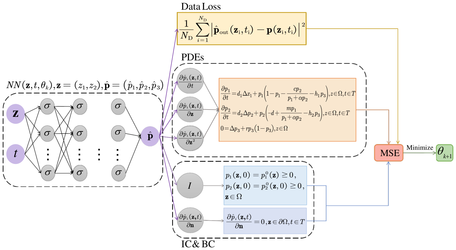
The iteration ends when a specific number of iterations is reached or a predetermined error threshold between the obtained successive solutions is satisfied. The PINN frame diagram and training process for solving singular systems proposed in this paper are shown in Figure 1.

4. Effectiveness of the PINN–Adam Model Under Overdevelopment Conditions

From Theorem 2, we get an analytical solution for the special case under the over-exploitation of the habitat. To investigate the capability of PINNs and traditional methods in solving models, two methods are used to solve PDEs in the spatiotemporal domain of $\mathcal{D}=\mathsf{\Omega }\times (0,T)$. Particularly, T is set in a range long enough to show the stability of the solution. After several tries, we select the parameter that T = 20, while the $\mathsf{\Omega }$ is set in $[0,1]\times [0,1]$.

In particular, the numerical values of equilibrium solutions and their spatial distribution in the results of equations are focused. According to Theorem 3, the parameters satisfy the necessary conditions for the existence of equilibrium solutions, as given by Formula (6).

In Section 4.1, we first focus on the solution of the PINN. And in Section 4.2, we present the traditional solution results, along with a comparison between the solution results of the PINN and traditional methods.

4.1. PINN Solution Results

In this section, we set up two cases that contain two situations in Theorem 3 and then solve them. The parameter settings are shown in

Table 2. Parameter under two simulated situations.

Situation	${\mathit{d}}_1$	${\mathit{d}}_2$	c	$\mathit{\alpha }$	d	m	${\mathit{h}}_1$	${\mathit{h}}_2$
Sit1	${10}^{-5}$	${10}^{-5}$	1.0	0.5	0.9	1.0	0.1	0.01
Sit2	${10}^{-5}$	${10}^{-5}$	0.8	1.2	0.5	1.0	0.1	0.2

, and the initial distributions for both cases are:

$$\begin{array}{c}\hfill p_1=0.5\times (si{n}^2\pi z_1+si{n}^2\pi z_2)+0.3\end{array}$$

(15)

$$\begin{array}{c}\hfill p_2=0.5\times (si{n}^2\pi z_1+si{n}^2\pi z_2)+0.2\end{array}$$

(16)

The parameters in Sit1 represent a situation where population $p_2$ is less affected by humans but has a higher population mortality. It also satisfies [Theorem 3, (S2)]. At the same time, the initial distribution (15) meets the Neumann boundary conditions and simulates the characteristic of higher density in the center of the region, which conforms to the law of nature.

This set of parameters satisfies the necessary conditions for the existence of an equilibrium solution (6), and the corresponding equilibrium solution is obtained as $u_{Sit1}^{*}$ = 0.7200, $v_{Sit1}^{*}$ = 0.1424 according to Formula (7).

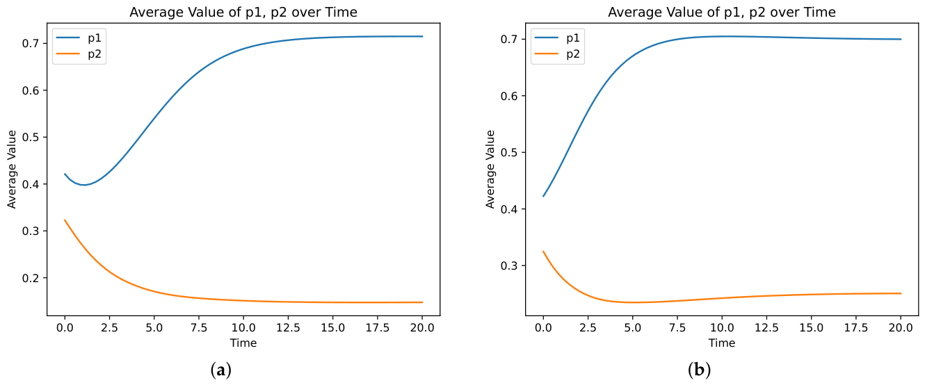
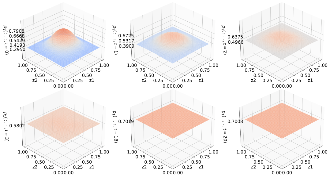
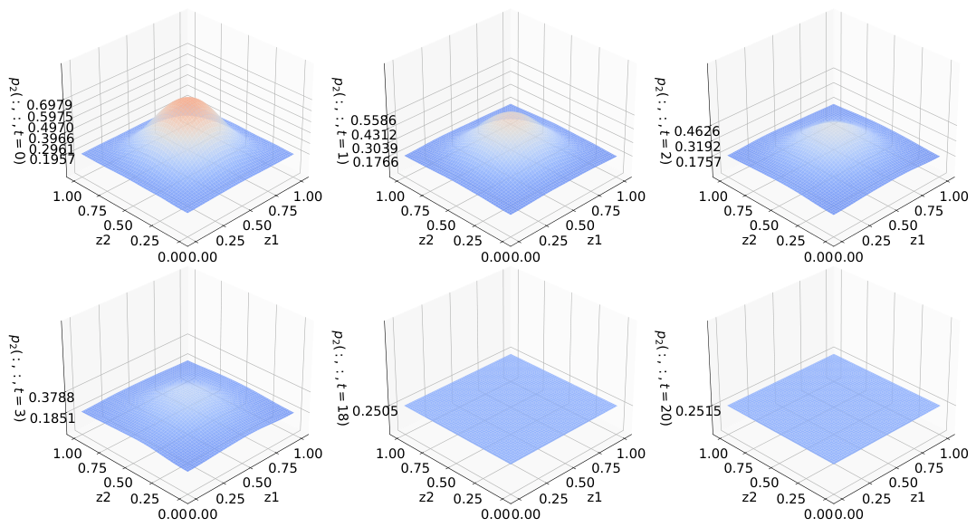
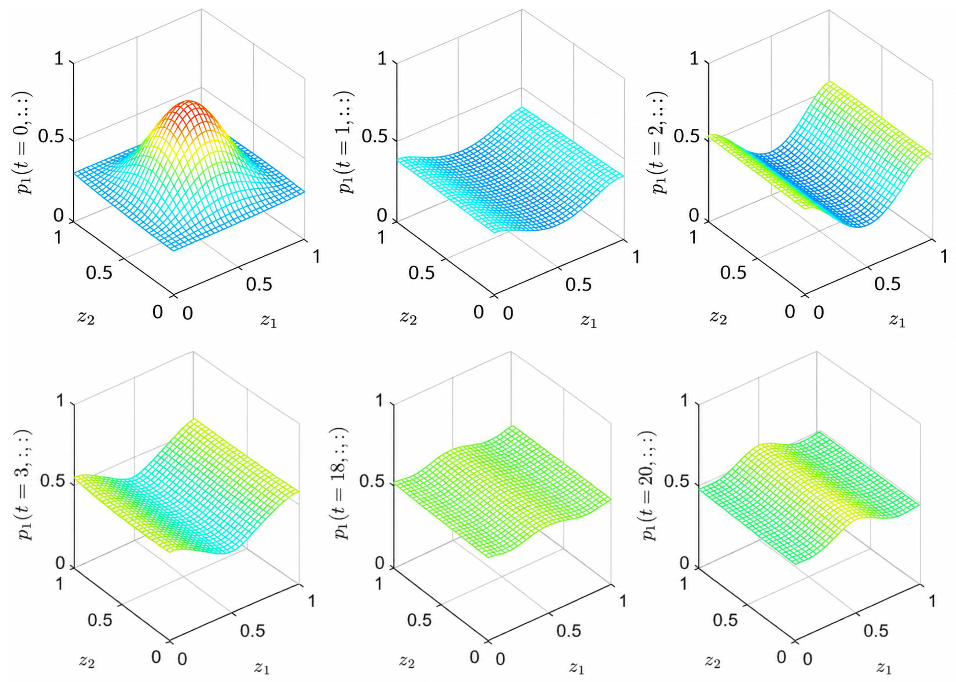
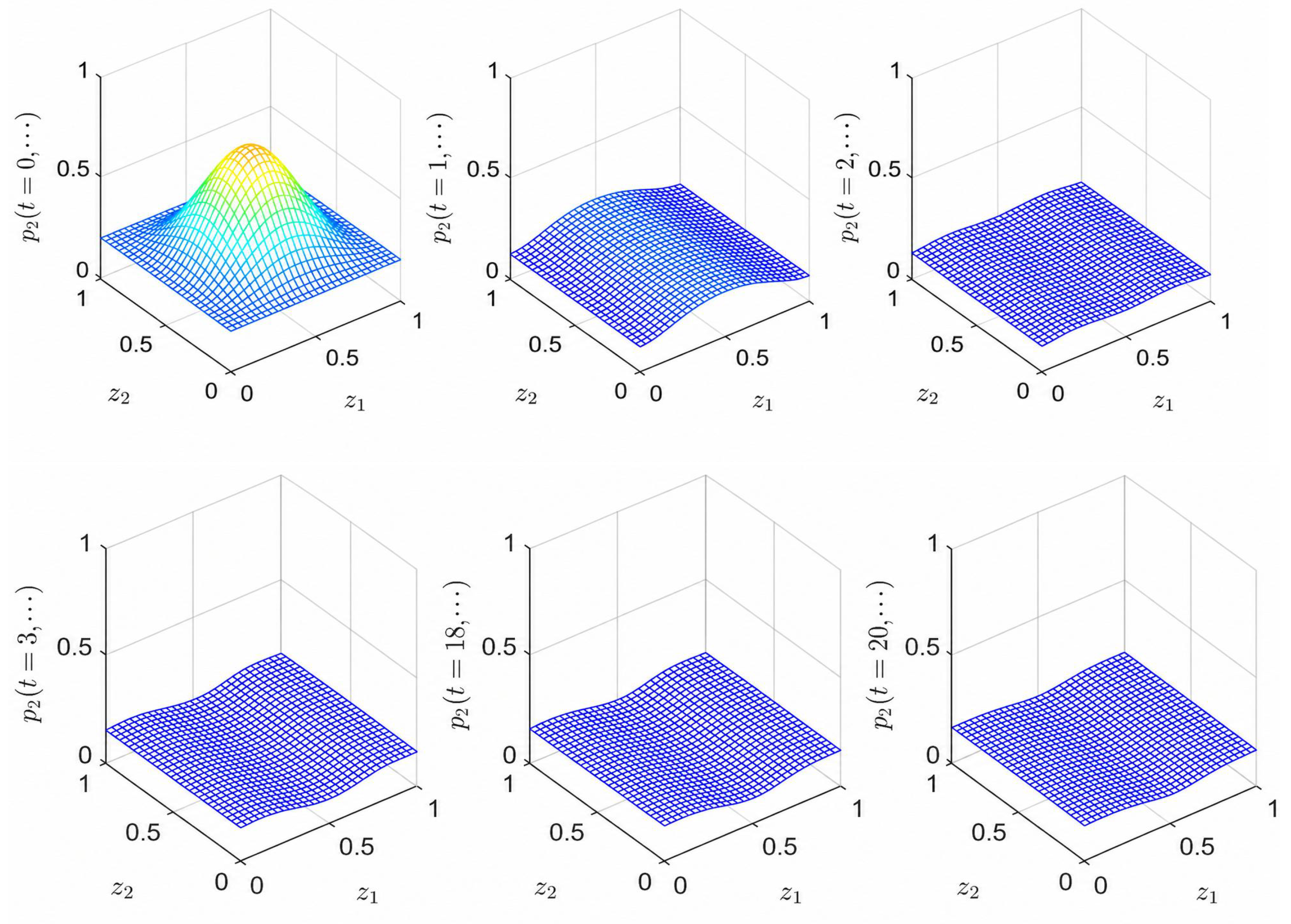
Under such conditions, we use 8000 periods of the Adam optimization scheme to train a PINN with five hidden layers and a width of 64 to solve the problem and obtain the results shown in Figure 2a,b. As shown in

Table 3. Sensitivity analysis of training epochs.

Epochs	Best Step	MAE	${\mathit{L}}_2$	${\mathit{L}}_{\mathit{\infty }}$	Training Time (s)
2000	2000	0.001271	0.132843	0.002922	165.577438
4000	4000	0.001076	0.120972	0.002439	325.022055
6000	6000	0.000572	0.069033	0.001710	485.468377
8000	7600	0.000601	0.071750	0.001761	640.489386
10,000	7600	0.000626	0.075353	0.001605	797.605144

, the prediction accuracy improves rapidly with increasing epochs in the early stage and gradually stabilizes after approximately 7600 steps. Although larger maximum epochs slightly improve the error metrics, the additional computational cost becomes significant. Therefore, 8000 epochs were selected to balance computational efficiency and model accuracy. To justify the selection of hyperparameters, a sensitivity analysis of the network architecture was conducted, as shown in

Table 4. Sensitivity analysis of network architecture.

Layers	Nodes	MAE	${\mathit{L}}_2$	${\mathit{L}}_{\mathit{\infty }}$
3	64	0.000343	0.041553	0.001046
4	64	0.000910	0.107489	0.003004
5	64	0.000216	0.025223	0.000573
5	128	0.000601	0.071750	0.001761
6	128	0.000631	0.072461	0.001795
7	128	0.000501	0.061083	0.001243

. Different combinations of hidden layers and neurons were tested under the same training settings. The architecture with five hidden layers and 64 neurons achieved the lowest MAE, $L_2$, and $L_{\infty }$ errors among all tested configurations. Therefore, this architecture was selected for the final simulations due to its superior accuracy and stability. It can be observed that population $p_1$ and population $p_2$ converge to the desired steady state in $\mathsf{\Omega }$ and remain stable in T, which is consistent with the result deduced in Section 3. The solution at $T=20$ is compared with the theoretical equilibrium solution with an error of 0.0054 and 0.0010.

For the second case, we select the parameters in Sit2, leaving the initial distribution and PINN unadjusted. It represents the situation that population $p_2$ is greatly affected by humans, but population mortality is low. It satisfies [Theorem 3, (S1)].

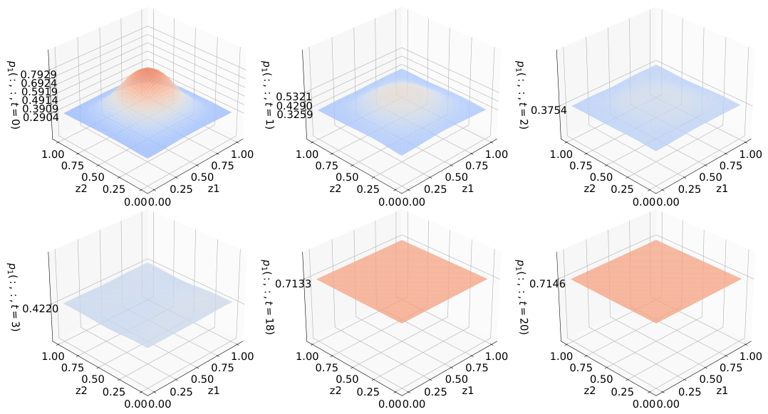
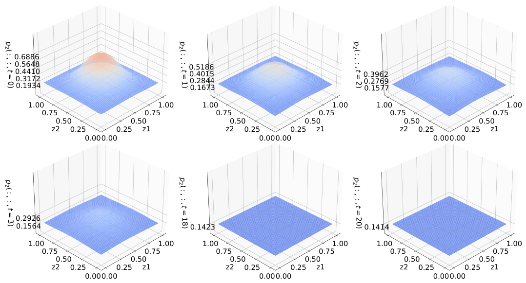
When the necessary conditions (6) are met, the results shown in Figure 3, Figure 4, Figure 5 and Figure 6 are obtained. Similar to the first case, with Formula (7), the results show a stable result in the spatial and temporal distributions of population density, and the error is 0.0008 and 0.0015 compared with the equilibrium solution $u_{Sit2}^{*}$ = 0.7000, $v_{Sit2}^{*}$ = 0.2500 calculated.

4.2. Traditional Methods and Comparison

For traditional baseline validation, conventional numerical analysis is standardly implemented utilizing a standard second-order piecewise nonlinear Galerkin finite element method for spatial discretization, which is sequentially coupled with an adaptive time-stepping scheme designed for stiff ordinary differential equations. Under initial and boundary conditions structurally analogous to those described in Section 4.1, and considering the severe numerical instabilities and grid-discretization stiffness that standard finite element meshes encounter when directly resolving full two-dimensional singular algebraic denominators, the comparative finite element scheme is projected onto a representative one-dimensional spatial domain mapped across thirty uniform fixed nodes while extending the temporal progression up to two hundred intervals to securely capture asymptotic behavior. This localized non-optimized grid distribution yields a total of six hundred thousand independent spatiotemporal tensor points requiring sequential algebraic evaluation, serving as a rigid baseline numerical benchmark that operates entirely without localized error estimators, advanced grid-optimization routines, or adaptive mesh refinement techniques. The corresponding numerical tracking trajectories are presented in Figure 7, Figure 8, Figure 9 and Figure 10 to illustrate the evolutionary trend under simplified geometric dimensions, demonstrating in sharp contrast that the proposed continuous physics-informed neural network model natively accommodates the full two-dimensional spatiotemporal singular coordinates and distribution pools without the necessity of dimensional reduction, grid dependencies, or complex mesh regeneration routines.

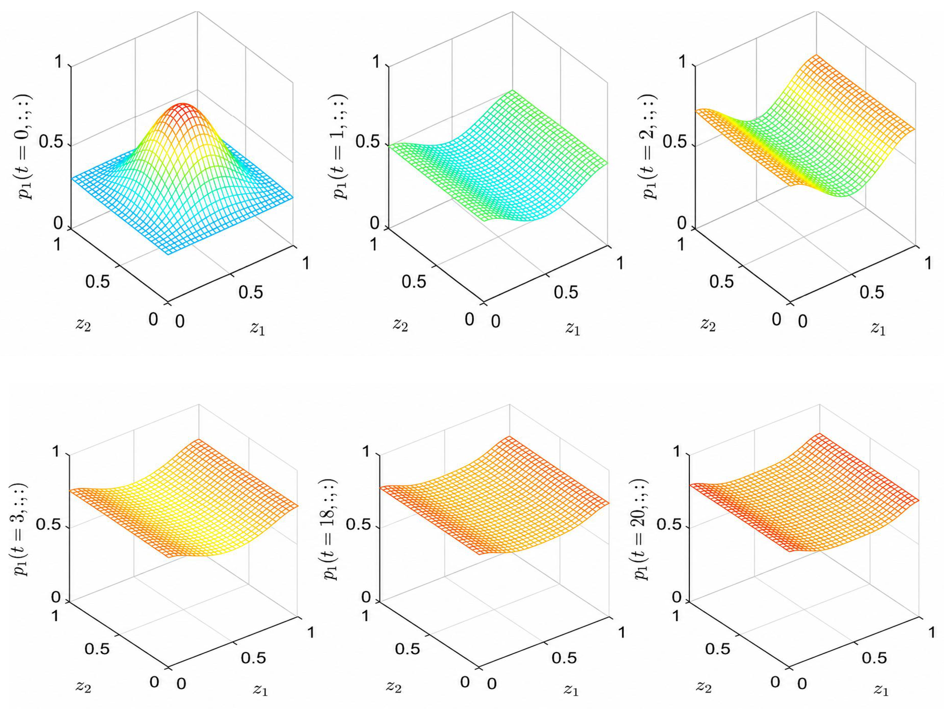
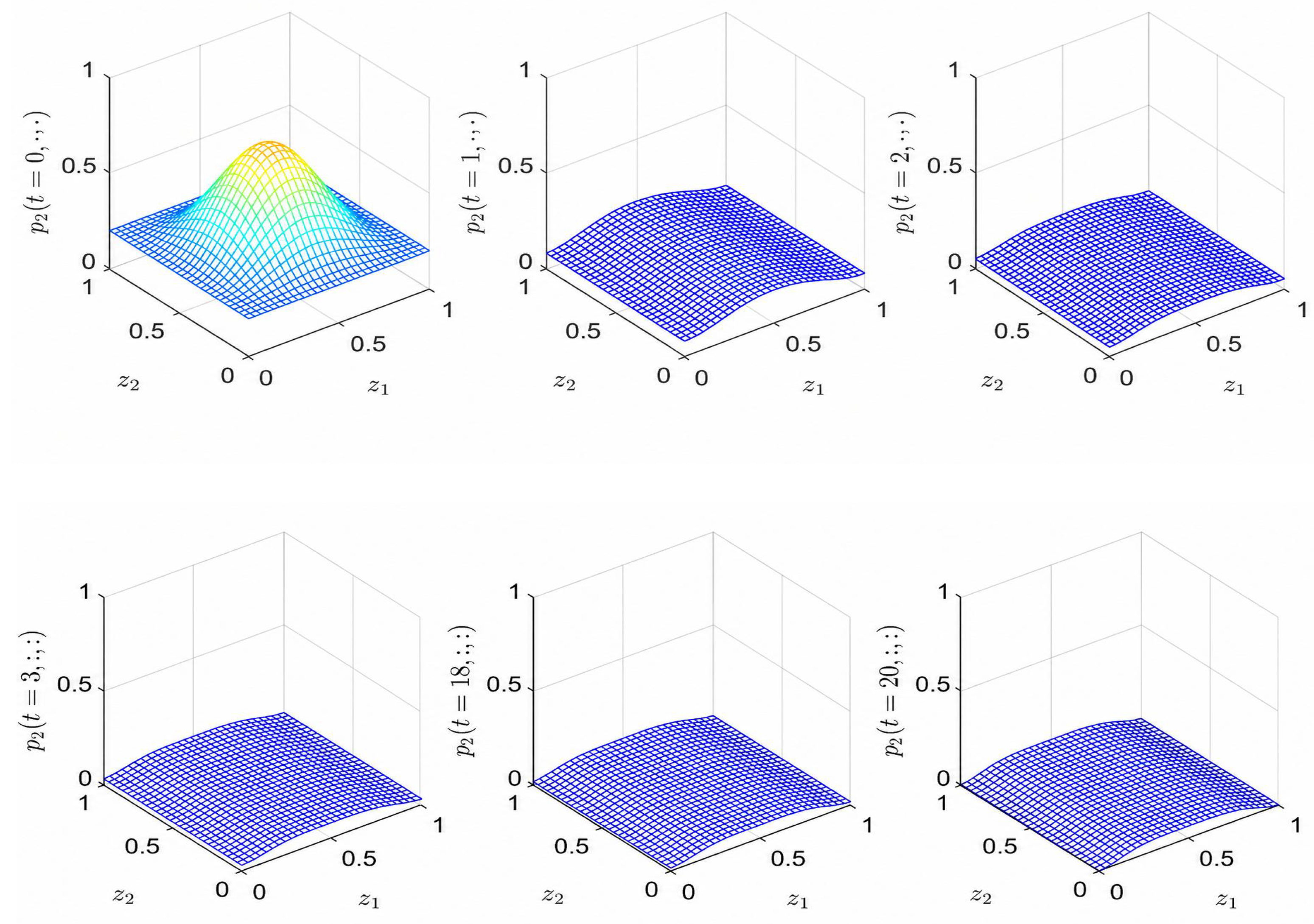
Observing Figure 7 and Figure 8, it can be found that the population has not stabilized within the time range shown in the figure. In Sit1, the average density at the final time point obtained by the FEM is $u_{Sit1}$ = 0.7398, $v_{Sit1}$ = 0.04440, as shown in Figure 9 and Figure 10. The error is 0.0198 and 0.098 compared to the equilibrium solution $u_{Sit1}^{*}$ = 0.7200, $v_{Sit1}^{*}$ = 0.1424, while the error of the PINN is only 0.0054 and 0.0010.

Under the condition of Sit2, the average density at the final time point is $u_{Sit2}$ = 0.5157, $v_{Sit2}$ = 0.1553, while the error is 0.1843 and 0.1018, compared to the equilibrium solution $u_{Sit2}^{*}$ = 0.7000, $v_{Sit2}^{*}$ = 0.2500. However, in the same case, the error of the PINN is only 0.0008 and 0.0015, which is more than 10 times less than the error of the FEM. Under the current implementation, PINN achieves notably lower errors compared to the FEM. While traditional methods such as the FEM can, in principle, achieve higher accuracy with mesh refinement and higher-order elements, such improvements typically come with rapidly increasing computational costs due to the curse of dimensionality. In contrast, PINN avoids mesh generation and demonstrates competitive accuracy with reduced memory requirements, making it a promising alternative for solving high-dimensional singular reaction-diffusion systems.

Table 5. The solution errors compared with the PINN and FEM.

Situation	Methods	MAE	${\mathit{L}}_2$ Norm	${\mathit{L}}_{\mathit{\infty }}$ Norm
Sit1	FEM	0.09687	3.065	0.1339
	PINN	0.0004273	0.07077	0.001291
Sit2	FEM	0.2115	6.387	0.50751
	PINN	0.0006581	0.03934	0.001436

shows the solving errors of the PINN and FEM. It can be seen from the table that the PINN is superior to the FEM in MAE, $L_2$, $L_{\infty }$ under two situations. Especially in the case of Sit2, the $L_2$ of the PINN is $6.116\times {10}^{-3}$ times that of the FEM, which indicates that the PINN is significantly better than traditional methods. In the case of Sit1, although the PINN is still excellent, it is not as good as the previous case. It might be that the PINN has more advantages in dealing with situations where there is low mortality and little influence by humans.

5. Application to Notolabrus Tetricus Population Prediction

In this section, we apply our model and assess the proposed PDE model by fitting its parameters to an actual biological dataset. Notolabrus tetricus is one of the most abundant fish species on the coastal coral reefs of South Australia [32], and it feeds on abalones, specifically Haliotis rubra, which is widely distributed in these reefs. First, we search for publicly available datasets and process the actual observational data. Population density and latitude–longitude data for both Notolabrus tetricus and Haliotis rubra are sourced from the publicly available datasets of the Australian Ocean Data Network (AODN). Second, we establish a two-dimensional spatial PDE model and utilize the PINN–Adam model to solve the inverse problem and obtain a fitter parameter. On a rectangular area defined by the geographical coordinates—the southwest corner at $43.5°$ S, $147.5°$ E, and the northeast corner at $42°$ S, $148.5°$ E—we selected data from 308 observation points within this rectangular area for the years 2006 and 2007 to evaluate the PDEs.

5.1. Data Source and Data Processing

To prevent spatial overfitting and manage computational complexity during neural network training, a proximity-based spatial density clustering and downsampling scheme is initially applied to the empirical observation infrastructure. The raw dataset encompasses three hundred and eight monitoring stations positioned along the South Australian coastline, which display substantial geographic density redundancy. By identifying contiguous observation nodes located within tight spatial proximity and clustering them based on geographic distance coordinates, a single representative station possessing the most comprehensive and continuous historical records is selected to act as the topological anchor for each localized cluster, thereby compressing the redundant monitoring array into seventy-one unique backbone stations. Following this spatial filtering and clustering pipeline, the population data are normalized by utilizing the historical maximum density observed across all functional stations as the environmental carrying capacity limit. To reconstruct the complete continuous spatial distributions of Notolabrus tetricus and Haliotis rubra across the domain, a linear radial basis function interpolation is subsequently performed on the filtered observation nodes, successfully smoothing out localized observational gaps while strictly preserving the authentic boundary geometry and coordinate alignment necessary for the subsequent stability analysis and physics-informed neural network evaluations. Moreover, the selection of linear radial basis functions for restoring continuous spatial distributions is deliberately customized to align with the intrinsic mathematical property of the downstream PINN–Adam framework. Linear RBF interpolation operates on the principle of geometric neutrality, constructing a smooth, unbiased baseline without injecting artificial high-order nonlinearities or subjective empirical priors that could conflict with the biological governing equations.

5.2. Parameters Fitness and Prediction

Based on Section 5.1, we select the population density data of Notolabrus tetricus for the years 2006 and 2007, and use the population spatial distributions of Notolabrus tetricus and Haliotis rubra as initial values. With $\mathsf{\Omega }=[0,1]\times [0,1],T=[0,10]$ as the spatial and temporal domains, we employ the PINN to solve the problem. The parameter settings are:

$$\begin{array}{c}\hfill d_1=0.001,d_2=0.001,c=1.0,\alpha =0.5,d=0.9,m=1.0,h_1=0.1,h_2=0.01,r=5.0\end{array}$$

(17)

The initial values of the parameters are provided to the PINN. The PINN is composed of five hidden layers, each consisting of 64 units, with the tanh activation function applied to all hidden layers. Considering the gradient descent optimization method, the PINN is trained using the Adam optimization scheme for 8000 epochs to obtain the solution. The optimal parameters obtained are:

$$\begin{array}{c}{d}_1=3.16\times {10}^{-3},d_2=1.32\times {10}^{-3},c=1.56,\alpha =0.671,h_1=1.10\times {10}^{-1},h_2=8.88\times {10}^{-3},\hfill \\ d=7.75\times {10}^{-1},m=1.06,r=4.99\hfill \end{array}$$

(18)

Considering the sensitivity of the inverse problem solution to historical data, we conduct multiple experiments.

Table 6. The mean and coefficient of variation for equation errors and parameters.

Parameters	MEAN	VAR	CV
$d_1$	$2.60\times {10}^{-3}$	$9.52\times {10}^{-7}$	$3.76\times {10}^{-1}$
$d_2$	$1.26\times {10}^{-3}$	$1.08\times {10}^{-8}$	$8.25\times {10}^{-2}$
c	$1.44$	$4.08\times {10}^{-2}$	$1.40\times {10}^{-2}$
$\alpha$	$7.17\times {10}^{-1}$	$6.35\times {10}^{-3}$	$1.11\times {10}^{-1}$
$h_1$	$1.11\times {10}^{-1}$	$3.00\times {10}^{-6}$	$1.56\times {10}^{-2}$
$h_2$	$8.58\times {10}^{-3}$	$2.7\times {10}^{-7}$	$6.06\times {10}^{-2}$
d	$7.97\times {10}^{-1}$	$1.49\times {10}^{-3}$	$4.85\times {10}^{-2}$
m	$1.04$	$8.33\times {10}^{-4}$	$2.77\times {10}^{-2}$
r	$4.99$	$9.23\times {10}^{-5}$	$1.93\times {10}^{-3}$

displays the equation errors, mean parameters, and coefficients of variation (CVs) obtained from multiple solution results. The CVs for all indicators are within a certain magnitude, demonstrating the stability of the solution results and parameters.

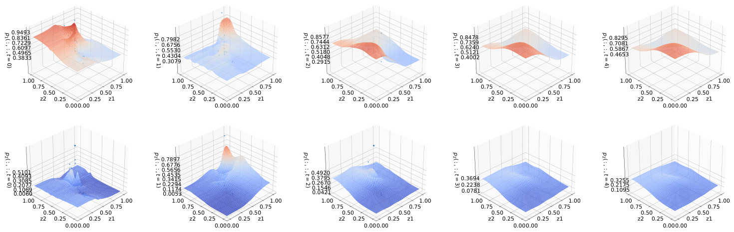
Figure 11 shows the solution results obtained from the model. The first three time points represent the fitting of real data, while the last two time points are predictions of the population density. The results demonstrate that in the actual population distribution, its evolution aligns with the equation’s pattern, and the existence of the equilibrium solution of the equation is independent of the initial conditions.

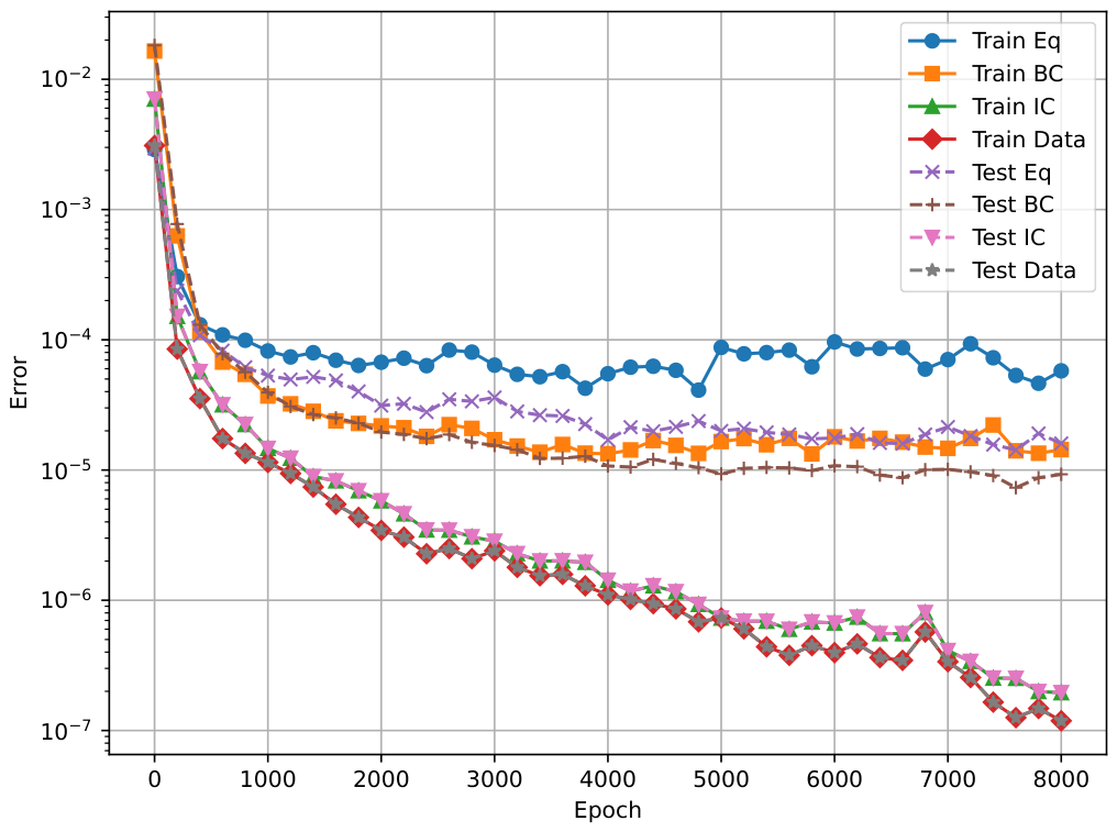
Figure 12 displays the convergence of the errors for various components of the equation during the training process of the PINN. Notably, the IC error is less than $1\times {10}^{-3}$. We observe that the error of the PINN method is less than ${10}^{-3}$, which shows a significant advantage compared with the error of the traditional finite element method. In our experiments, under the same initial conditions and parameters, the error of the FEM is usually between ${10}^{-2}$ and ${10}^{-3}$, which is significantly higher than the result of the PINN method, indicating that the PINN is capable of fitting the real-world scenario with high accuracy.

Regarding the operational assumption of simplifying the human factor to a constant value of $p_3\equiv 1$ during the empirical simulation pipeline, it is crucial to recognize that while this elimination of dynamic anthropogenic pressure serves as a baseline configuration, it introduces a specific simplification drawback concerning real-world ecological feedback loops. This decoupling was primarily enforced in the numerical experiments to establish a controlled mathematical benchmark, thereby isolating the pure reaction–diffusion spatiotemporal dynamics of the predator and prey fish populations without the confounding, fast-scale variations typically introduced by dynamic harvesting metrics. To mitigate this structural limitation and enhance the ecological realism of the model, future mathematical expansions must reintroduce time-dependent or density-gradient-based human fishing terms to capture the coupled, long-term evolution between economic incentives, policy regulations, and marine biomass stability.

6. Conclusions

We have proposed an improved prey–predator model that considers the impact of human activities on the population system. Due to the singularity of the system, the conditions for equilibrium existence are discussed, and a solution formula for a specific case is presented. A physics-informed neural network (PINN), with attention paid to its iterative methods and activation function, is used to solve these 2D singular PDE systems. Compared with traditional finite element methods, the PINN exhibits more than a 10-fold improvement in the accuracy of population density estimation across different parametric conditions. The Mean Absolute Error (MAE) of the model when choosing the PINN is reduced by 99%. The simulation cases demonstrate that the PINN exhibits superior performance in 2D space compared to traditional methods. Finally, the model is evaluated under real-world conditions, validating its effectiveness in modeling fish data from coral reefs along the coast of South Australia. On the test set, the Mean Squared Error (MSE) reaches $1.93\times {10}^{-3}$, which proves the good solving capability of the PINN. In summary, utilizing the PINN to solve the newly proposed model is effective in high-dimensional spaces and can be well applied to real ecological environments, providing valuable insights and references for understanding actual ecological phenomena. In addition to its theoretical contributions, the proposed framework provides a practical tool for analyzing and predicting spatiotemporal dynamics in real ecological systems. In particular, it can be applied to evaluate the impact of human activities on species interactions, predict population evolution under different environmental conditions, and support decision-making in ecological conservation and resource management. Moreover, the proposed PINN-based approach offers a flexible and efficient alternative for solving high-dimensional PDE systems, and can be extended to other application domains such as environmental modeling, epidemiology, and complex physical processes.

In terms of future research perspectives, several promising directions warrant further exploration to expand the scope and impact of this framework. First, while the current system relies on the theoretical smoothness of solutions to bypass singular regions, future work should develop self-adaptive or dynamic loss-weighting mechanisms, such as learning rate annealing or residual-based attention, to automatically balance the severe gradient disparities near singular manifolds when dealing with harsher singular systems. Furthermore, since real-world marine ecosystems, like reef fish habitats, are inherently subject to stochastic environmental fluctuations and anthropogenic seasonal shifts, integrating our current deterministic 2D reaction–diffusion model into a stochastic partial differential equation framework solved via physics-informed generative adversarial networks represents a vital subsequent step. However, the reliance on a relatively brief temporal sequence for real-world fish population verification remains a bottleneck of the current stage of this work. To address this, as more extensive longitudinal ecological monitoring programs mature along the South Australian coast, we aim to extend the forecasting horizon by incorporating multi-year, high-frequency temporal data into the PINN–Adam framework, thereby allowing for a more rigorous assessment of the model’s long-term predictive stability. Lastly, to eliminate the need for retraining whenever initial spatial distributions change, future endeavors will focus on implementing advanced operator learning architectures such as Fourier neural operators or deep operator networks to learn the entire solution operator, thereby facilitating instantaneous, zero-shot ecological forecasting and real-time decision-making for wildlife conservation and marine resource management.

References

1. Zienkiewicz, O.C. Achievements and some unsolved problems of the finite element method. Int. J. Numer. Methods Eng. 2000, 47, 9–28. [Google Scholar] [CrossRef] [Scilit]
2. Versteeg, H.; Malalasekera, W. The finite volume method. In An Introduction to Computational Fluid Dynamics; John Wiley & Sons: New York, NY, USA, 1995; pp. 102–206. [Google Scholar]
3. Onate, E.; Roger, O. (Eds.) Particle-Based Methods: Fundamentals and Applications; Springer Science & Business Media: Berlin/Heidelberg, Germany, 2011. [Google Scholar]
4. Bürchner, T.; Kopp, P.; Kollmannsberger, S.; Rank, E. Isogeometric multi-resolution full waveform inversion based on the finite cell method. Comput. Methods Appl. Mech. Eng. 2023, 417, 116286. [Google Scholar] [CrossRef] [Scilit]
5. Michael, I.; Dirk, P. MooAFEM: An object oriented Matlab code for higher-order adaptive FEM for (nonlinear) elliptic PDEs. Appl. Math. Comput. 2023, 442, 127731. [Google Scholar] [CrossRef] [Scilit]
6. Raissi, M.; Perdikaris, P.; Karniadakis, G. Physics-informed neural networks: A deep learning framework for solving forward and inverse problems involving nonlinear partial differential equations. J. Comput. Phys. 2019, 378, 686–707. [Google Scholar] [CrossRef] [Scilit]
7. Yan, X.B.; Xu, Z.Q.J.; Ma, Z. Laplace-based fractional physics-informed neural networks for solving forward and inverse problems of subdiffusion. arXiv 2023, arXiv:2304.00909. [Google Scholar]
8. Zhao, C.; Zhang, F.; Lou, W.; Wang, X.; Yang, J. A comprehensive review of advances in physics-informed neural networks and their applications in complex fluid dynamics. Phys. Fluids 2024, 36, 101301. [Google Scholar] [CrossRef] [Scilit]
9. Liu, Y.; Dongkun, Z.; Karniadakis, G.E. Physics-informed generative adversarial networks for stochastic differential equations. SIAM J. Sci. Comput. 2020, 42, A292–A317. [Google Scholar] [CrossRef] [Scilit]
10. Wang, Y.; Wang, H.; Zhang, S. Quantifying prediction and intervention measures for PM2.5 by a PDE model. J. Clean. Prod. 2020, 268, 122131. [Google Scholar] [CrossRef] [Scilit]
11. Farmer, J.; Oian, C.A.; Bowman, B.A.; Khan, T. Empirical loss weight optimization for PINN modeling laser bio-effects on human skin for the 1D heat equation. Mach. Learn. Appl. 2024, 16, 100563. [Google Scholar] [CrossRef] [Scilit]
12. Priyadarshi, G.; Murali, C.; Agarwal, S.; Naik, B.K. Parametric investigation and optimization of phase change material-based thermal energy storage integrated desiccant coated energy exchanger through physics informed neural networks oriented deep learning approach. J. Energy Storage 2024, 80, 110231. [Google Scholar] [CrossRef] [Scilit]
13. Zhang, T.; Yan, R.; Zhang, S.; Yang, D.; Chen, A. Application of Fourier feature physics-information neural network in model of pipeline conveying fluid. Thin-Walled Struct. 2024, 198, 111693. [Google Scholar] [CrossRef] [Scilit]
14. Xu, C.; Cao, B.T.; Yuan, Y.; Meschke, G. Transfer learning based physics-informed neural networks for solving inverse problems in engineering structures under different loading scenarios. Comput. Methods Appl. Mech. Eng. 2023, 405, 115852. [Google Scholar] [CrossRef] [Scilit]
15. González-Gaxiola, O.; Hart-Simmons, M.; Ahmed, H.M.; Biswas, A. A Novel Neural Network-Based Symbolic Approach for Shallow-Water Waves with Surface Tension. Fluids 2026, 11, 100. [Google Scholar] [CrossRef] [Scilit]
16. Liu, K.; Wu, J. Dual Adaptive Neural Network for Solving Free-Flow Coupled Porous Media Models Under Unique Continuation Problem. Computation 2025, 13, 228. [Google Scholar] [CrossRef] [Scilit]
17. Zhang, Y.; Zhang, R.F.; Yuen, K.V. Neural network-based analytical solver for Fokker-Planck equation. Eng. Appl. Artif. Intell. 2023, 125, 106721. [Google Scholar] [CrossRef] [Scilit]
18. Peng, S.; Yang, S.; Gao, B.; Liu, W.; Wang, F.; Tang, Z. Prediction of 3D temperature field through single 2D temperature data based on transfer learning-based PINN model in laser-based directed energy deposition. J. Manuf. Process. 2025, 138, 140–156. [Google Scholar] [CrossRef] [Scilit]
19. Skellam, J. Random dispersal in theoretical populations. Bull. Math. Biol. 1991, 53, 135–165. [Google Scholar] [CrossRef] [Scilit]
20. Escudero, C.; Buceta, J.; de la Rubia, F.J.; Lindenberg, K. Extinction in population dynamics. Phys. Rev. E 2004, 69, 021908. [Google Scholar] [CrossRef] [Scilit]
21. Wang, W.; Liu, Q.X.; Jin, Z. Spatiotemporal complexity of a ratio-dependent predator-prey system. Phys. Rev. E 2007, 75, 051913. [Google Scholar] [CrossRef] [Scilit] [PubMed]
22. Ko, W.; Ahn, I. A diffusive one-prey and two-competing-predator system with a ratio-dependent functional response: I, long time behavior and stability of equilibria. J. Math. Anal. Appl. 2013, 397, 9–28. [Google Scholar] [CrossRef] [Scilit]
23. Chen, W.; Wang, M. Qualitative analysis of predator-prey models with Beddington-DeAngelis functional response and diffusion. Math. Comput. Model. 2005, 42, 31–44. [Google Scholar] [CrossRef] [Scilit]
24. Pauly, D. Anecdotes and the shifting baseline syndrome of fisheries. Trends Ecol. Evol. 1995, 10, 430. [Google Scholar] [CrossRef] [Scilit] [PubMed]
25. Jackson, J.B.; Kirby, M.X.; Berger, W.H.; Bjorndal, K.A.; Botsford, L.W.; Bourque, B.J.; Warner, R.R. Historical overfishing and the recent collapse of coastal ecosystems. Science 2001, 293, 629–637. [Google Scholar] [CrossRef] [Scilit]
26. Jiang, Y.; Zhang, Q.; Wang, H. Modeling boyciana–fish–human interaction with partial differential algebraic equations. Math. Biosci. 2016, 277, 141–152. [Google Scholar] [CrossRef] [Scilit]
27. Leshno, M.; Lin, V.Y.; Pinkus, A.; Schocken, S. Multilayer feedforward networks with a nonpolynomial activation function can approximate any function. Neural Netw. 1993, 6, 861–867. [Google Scholar] [CrossRef] [Scilit]
28. Ramachandran, P.; Zoph, B.; Le, Q.V. Searching for Activation Functions. arXiv 2017, arXiv:1710.05941. [Google Scholar] [CrossRef] [Scilit]
29. Rahaman, N.; Baratin, A.; Arpit, D.; Draxler, F.; Lin, M.; Hamprecht, F.A.; Bengio, Y.; Courville, A. On the Spectral Bias of Neural Networks. In Proceedings of the 36th International Conference on Machine Learning; PMLR: New York, NY, USA, 2019; Volume 97, pp. 5301–5310. [Google Scholar]
30. Kingma, D.P.; Ba, J. Adam: A Method for Stochastic Optimization. arXiv 2014, arXiv:1412.6980. [Google Scholar]
31. He, Q.; Barajas-Solano, D.; Tartakovsky, G.; Tartakovsky, A.M. Physics-informed neural networks for multiphysics data assimilation with application to subsurface transport. Adv. Water Resour. 2020, 141, 103610. [Google Scholar] [CrossRef] [Scilit]
32. Shepherd, S.A.; Clarkson, P.S. Diet, feeding behaviour, activity and predation of the temperate blue-throated wrasse, Notolabrus tetricus. Mar. Freshw. Res. 2001, 52, 311–322. [Google Scholar] [CrossRef] [Scilit]
Figure 1. Framework about the PINNs.
Mathematics 14 02148 g001
Figure 2. Evolution of the average density of population p 1 and population p 2 , taking values as in two situations. (a) Evolution of the average density of population p 1 and population p 2 in Sit1 in Table 3. (b) Evolution of the average density of population p 1 and population p 2 in Sit2 in Table 3.
Mathematics 14 02148 g002
Figure 3. The evolution of population density p 1 under parameter setting Sit1 in Table 3.
Mathematics 14 02148 g003
Figure 4. The evolution of population density p 2 under parameter setting Sit1 in Table 3.
Mathematics 14 02148 g004
Figure 5. The evolution of population density p 1 under parameter setting Sit2 in Table 3.
Mathematics 14 02148 g005
Figure 6. The evolution of population density p 2 under parameter setting Sit2 in Table 3.
Mathematics 14 02148 g006
Figure 7. The evolution of population density p 1 under parameter setting Sit1 in Table 3.
Mathematics 14 02148 g007
Figure 8. The evolution of population density p 2 under parameter setting Sit1 in Table 3.
Mathematics 14 02148 g008
Figure 9. The evolution of population density p 1 under parameter setting Sit2 in Table 3.
Mathematics 14 02148 g009
Figure 10. The evolution of population density p 2 under parameter setting Sit2 in Table 3.
Mathematics 14 02148 g010
Figure 11. (Top row): the evolution of the density of p 1 ; (bottom row): the evolution of the density of p 2 .
Mathematics 14 02148 g011
Figure 12. PDE errors of the model during the training.
Mathematics 14 02148 g012