Matched–Mismatched Uncertainty Compensation in Dynamic SMC Using Optimal Fractional Loop-Transfer-Recovery Observer

Abstract

A new fractional dynamic sliding mode control (FD-SMC) framework is introduced to reduce chattering in the control of fractional-order chaotic systems. In this method, chattering is eliminated by placing a fractional integrator before the system control input. As a result, the augmented system has a higher dimension than the original system, meaning that additional states are introduced. Effective control therefore requires identifying or estimating these new states or the corresponding plant model. To address this issue, a robust optimal fractional loop-transfer-recovery observer (ROF-LTRO) is developed. Furthermore, the key advantage of sliding mode control (SMC)—its invariance to matched uncertainties—is often lost in many plants such as chaotic systems, because many of them contain mismatched uncertainties. To restore and extend the invariance property, multiple sliding surfaces combined with a virtual control input are employed. In addition, the proposed FD-SMC and ROF-LTRO do not rely on prior knowledge of uncertainty bounds, which is beneficial for practical implementation. Then, a two-stage design procedure based on two-surface definition is presented, and simulation results are provided for the extended fractional Duffing–Holmes chaotic system (EF-DHCS) under both matched and mismatched uncertainties.

1. Introduction

The motivation for using sliding mode control (SMC) lies in its invariance property, which enables robust performance in the presence of uncertainties and disturbances—despite the practical challenges of implementing SMC in real systems [1,2]. Among the characteristics of SMC, invariance is considered stronger than general robustness [1,3]. However, SMC faces two major issues: chattering and mismatched uncertainties.

Chattering refers to small-amplitude, high-frequency but finite oscillations that can damage mechanical and electrical components [1]. Four main design strategies have been introduced to mitigate chattering, namely, boundary-layer SMC (BL-SMC), adaptive boundary-layer SMC (ABL-SMC), higher-order SMC (HO-SMC), and dynamic SMC (D-SMC) [1], as well as intelligent approaches such as fuzzy [4,5].

BL-SMC and ABL-SMC fail to preserve the invariance property [4,5,6,7]. HO-SMC can reduce chattering by shifting switching effects to higher-order derivatives of the output [8,9,10], and several algorithms exist for implementing second-order [11,12,13] and higher-order SMC [9,10]. However, HO-SMC typically requires knowledge or estimation of higher-order derivatives of the plant model [8,9,10,11,12,13], which is a major limitation. For instance, when the relative degree is two, model derivatives must often be estimated using observers such as sliding differentiators [8]. However, in D-SMC, an integrator (or another strictly low-pass filter) is placed before the plant input [14,15], effectively filtering out high-frequency switching and eliminating chattering [15,16,17,18,19]. However, this increases the system order by one, meaning that the augmented model must be fully known for SMC design [17,19]. Thus, D-SMC requires the plant model, whereas HO-SMC requires its derivatives—giving D-SMC an advantage.

Fuzzy approaches are generally classified into two categories: direct and indirect. In direct approaches, the fuzzy system functions as the main controller, whereas in indirect approaches, the fuzzy system plays a secondary or supportive role within the controller structure [20].

Uncertainties also significantly affect system stability, performance, and robustness [3,21]. When uncertainty enters through the input channel, it is classified as matched; otherwise, it is mismatched [21]. Mismatched uncertainties remove the invariance property of SMC [21], prompting extensive research [22,23,24,25,26,27,28,29,30,31,32,33,34,35,36,37,38,39,40,41,42,43]. Yet, many approaches still suffer from chattering because the Sign function appears directly in the control input [22,23,24,25,26,27,28,29,30,31]. Some methods are conceptually or practically complex [23,34], while others apply only to linear systems [23,33]. Several works rely on known uncertainty bounds [35,36,37], disturbance observers [26], sliding differentiators [29], or extended state observers [28]. Other approaches minimize mismatched uncertainty effects using LMI-based techniques [38] or employ multiple sliding surfaces [39,40], though chattering persists in [41,42,43]. Moreover, multiple sliding surfaces are used in some works [43], in which the Sign function is directly available in control signal. Finally, some works are based on fuzzy systems [44,45,46]. But comparison of fuzzy-based and non-fuzzy-based controllers is not reliable.

Fractional calculus has gained attention due to its effectiveness in modeling dynamical systems, including chaotic systems [47]. Fractional-order models can accurately describe many physical, mathematical, and engineering processes [48,49,50]. This has led to developments in fractional stability theory [51,52], fractional controllers, and identification methods [53]. Fractional sliding mode control (F-SMC) has emerged due to its invariance properties [54]. Examples include adaptive F-SMC [54], integral SMC for fractional chaotic tracking [55], terminal F-SMC for synchronization [56], fractional higher-order SMC (FHO-SMC) based on PI control [57], and diffusive-representation-based FHO-SMC [58]. Output-feedback F-SMC for unknown fractional chaotic systems is proposed in [59], and an LQR-based F-SMC appears in [60]. However, chattering remains a central challenge across these works. Therefore, the main goal of this study is to present a new fractional dynamic sliding mode (FD-SMC) method. Then, the plant model should be identified using an observer.

Generally, the main objective of the observer design is to utilize the known system inputs and outputs to estimate unmeasurable system parts. The output of the observer and the main system is used as feedback for the observer to reform it [61,62,63,64,65,66,67]. The identification concept consists of a wide range in system control such as state observer [61,62,67], disturbance observer [63] and model identification [64,65,66,67]. It is worth mentioning that the main drawback of these observers is their need to have knowledge of the system model upper bound.

To address both chattering and mismatched uncertainties in fractional-order chaotic systems, this study combines multiple sliding surfaces with a new fractional dynamic SMC (FD-SMC) framework. Because FD-SMC requires estimation of the sliding surface, we introduce a robust optimal fractional loop-transfer-recovery observer (ROF-LTRO) to estimate the unknown components. This ensures that the sliding surface is fully available. The proposed method is conceptually simple, does not require uncertainty bounds in either FD-SMC or ROF-LTRO, and is therefore well-suited for practical implementation. To demonstrate its advantages, we apply it to an extended fractional Duffing–Holmes chaotic system (EF-DHCS) with both matched and mismatched uncertainties.

The main contributions of this paper are as follows:

• A new FD-SMC structure is introduced.
• Chattering is eliminated through the FD-SMC framework.
• A new ROF-LTRO scheme is developed to estimate unknown uncertainties.
• An EF-DHCS with matched and mismatched uncertainties is constructed.
• The proposed method effectively handles mismatched uncertainties.

The remainder of the paper is organized as follows: Section 2 presents the problem formulation; Section 3 details the ROF-LTRO design; Section 4 discusses the control input design; and Section 5 and Section 6 provide simulation results and conclusions.

2. Problem Formulation

Definition 1.

Caputo q-order differentiation and integration of function $\mathrm{g}(\mathrm{t})$ with respect to time $\mathrm{t}$ are denoted by [67,68]:

$${\mathrm{D}}_{{\mathrm{t}}_0}^{\mathrm{q}}\mathrm{g}(\mathrm{t})={\displaystyle \frac{1}{\Gamma (1-\mathrm{q})}}{\displaystyle {\int }_{{\mathrm{t}}_0}^{\mathrm{t}}\frac{{\mathrm{g}}^{\prime }(\mathrm{\tau })}{{(\mathrm{t}-\mathrm{\tau })}^{\mathrm{q}}}}\mathrm{d}\mathrm{\tau }$$

(1)

$${\mathrm{I}}_{{\mathrm{t}}_0}^{\mathrm{q}}\mathrm{g}(\mathrm{t})={\displaystyle \frac{1}{\Gamma (\mathrm{q})}}{\displaystyle {\int }_{{\mathrm{t}}_0}^{\mathrm{t}}{(\mathrm{t}-\mathrm{\tau })}^{\mathrm{q}-1}\mathrm{g}(\mathrm{\tau })}\mathrm{d}\mathrm{\tau }$$

(2)

where $\mathrm{t}>{\mathrm{t}}_0$ and $0<\mathrm{q}<1$ are time series and degree of differentiating, respectively, and $\Gamma (\mathrm{q})$ is the Gamma function defined as $\Gamma (\mathrm{q})={\displaystyle {\int }_0^{\infty }{\mathrm{\tau }}^{\mathrm{q}-1}{\mathrm{e}}^{-\mathrm{\tau }}\mathrm{d}\mathrm{\tau }}$.

Remark 1.

From here and in the continuation of this paper, we suppose that the initial time of fractional derivative is zero, i.e., ${\mathrm{t}}_0=0$. Moreover, for simplicity, the subscript ${\mathrm{t}}_0$ is also eliminated and hence we write ${\mathrm{D}}^{\mathrm{q}}$ and ${\mathrm{I}}^{\mathrm{q}}$ instead of ${\mathrm{D}}_{{\mathrm{t}}_0}^{\mathrm{q}}$ and ${\mathrm{I}}_{{\mathrm{t}}_0}^{\mathrm{q}}$.

Theorem 1.

For a constant $\mathrm{g}(\mathrm{t})=\mathrm{k}$ one can write:

$${\mathrm{I}}^{\mathrm{q}}\mathrm{k}={\displaystyle \frac{\mathrm{k}{\mathrm{t}}^{\mathrm{q}}}{\mathrm{q}\Gamma (\mathrm{q})}}$$

(3)

Proof. 

According to (2), we have:

$${\mathrm{I}}^{\mathrm{q}}\mathrm{k}={\displaystyle \frac{1}{\Gamma (\mathrm{q})}}{\displaystyle {\int }_{{\mathrm{t}}_0}^{\mathrm{t}}{\left(\mathrm{t}-\mathrm{\tau }\right)}^{\mathrm{q}-1}\mathrm{k}}\mathrm{d}\mathrm{\tau }={\displaystyle \frac{\mathrm{k}}{\Gamma (\mathrm{q})}}{\displaystyle {\int }_{{\mathrm{t}}_0}^{\mathrm{t}}{\left(\mathrm{t}-\mathrm{\tau }\right)}^{\mathrm{q}-1}}\mathrm{d}\mathrm{\tau }=\left.{\displaystyle \frac{-\mathrm{k}}{\mathrm{q}\Gamma (\mathrm{q})}}{\left(\mathrm{t}-\mathrm{\tau }\right)}^{\mathrm{q}}\right|\begin{array}{c}\mathrm{t}\\ 0\end{array}={\displaystyle \frac{\mathrm{k}{\mathrm{t}}^{\mathrm{q}}}{\mathrm{q}\Gamma (\mathrm{q})}}$$

(4)

Now consider a class of fractional chaotic system as follows:

$$\begin{array}{l}{\mathrm{D}}^{\mathrm{q}}{\mathrm{x}}_1={\mathrm{x}}_2+{\mathrm{f}}_1(\mathrm{x},\mathrm{t})\\ {\mathrm{D}}^{\mathrm{q}}{\mathrm{x}}_2=\mathrm{v}+{\mathrm{f}}_2(\mathrm{x},\mathrm{t})\end{array}$$

(5)

Let $\mathrm{x}={[{\mathrm{x}}_1,{\mathrm{x}}_2]}^{\mathrm{T}}$ denote the accessible system state vector, $\mathrm{y}={\mathrm{x}}_1$ the system output, and $\mathrm{v}$ the control input, and let ${\mathrm{f}}_1$ and ${\mathrm{f}}_2$ represent the unknown matched and mismatched uncertainties, respectively. The system output is given by $\mathrm{y}$. The objective is to design the control input $\mathrm{v}$ using a chattering-free FD-SMC scheme such that $\mathrm{y}={\mathrm{x}}_1$ converges to zero despite the presence of uncertainties $\mathrm{f}={[{\mathrm{f}}_1,{\mathrm{f}}_2]}^{\mathrm{T}}$, while preserving the invariance property. As previously noted, because the system contains mismatched uncertainty ${\mathrm{f}}_1$, fractional traditional SMC (FT-SMC) is not applicable. To address this challenge, FD-SMC with multiple sliding surfaces is adopted. The first step is to apply a state-feedback transformation to system (5) of the form $\mathrm{v}={\mathrm{a}}_1{\mathrm{x}}_1+{\mathrm{a}}_2{\mathrm{x}}_2+\mathrm{u}$, where ${\mathrm{a}}_1$ and ${\mathrm{a}}_2$ are constants, and $\mathrm{u}$ is the new control input to be designed.

$$\begin{array}{l}{\mathrm{D}}^{\mathrm{q}}{\mathrm{x}}_1={\mathrm{x}}_2+{\mathrm{f}}_1(\mathrm{x},\mathrm{t})\\ {\mathrm{D}}^{\mathrm{q}}{\mathrm{x}}_2={\mathrm{a}}_1{\mathrm{x}}_1+{\mathrm{a}}_2{\mathrm{x}}_2+\mathrm{u}+{\mathrm{f}}_2(\mathrm{x},\mathrm{t})\end{array}$$

(6)

Refer to the first part of (6):

$${\mathrm{D}}^{\mathrm{q}}{\mathrm{x}}_1={\mathrm{x}}_2+{\mathrm{f}}_1(\mathrm{x},\mathrm{t})$$

(7)

In the first step, we can consider the state ${\mathrm{x}}_2$ as the virtual input control signal of (7) and therefore, we calculate a smooth ${\mathrm{x}}_2$ (called desired ${\mathrm{x}}_2$ or ${\mathrm{x}}_{\mathrm{d}2}$) such that $\mathrm{y}={\mathrm{x}}_1$ converges to zero. In this case, uncertainty ${\mathrm{f}}_1(\mathrm{x},\mathrm{t})$ is matched with respect to ${\mathrm{x}}_2$. Therefore, we define the following sliding surface.

$${\mathrm{s}}_1=\mathrm{k}{\mathrm{X}}_1,{\mathrm{X}}_1={[{\mathrm{x}}_1,{\mathrm{D}}^{\mathrm{q}}{\mathrm{x}}_1,{\mathrm{D}}^{2\mathrm{q}}{\mathrm{x}}_1]}^{\mathrm{T}},\mathrm{k}=[{\mathrm{k}}_1,{\mathrm{k}}_2,{\mathrm{k}}_3]$$

(8)

The coefficients ${\mathrm{k}}_1,{\mathrm{k}}_2,{\mathrm{k}}_3$ are properly chosen such that the zero dynamics of sliding surface would be stable; i.e., ${\mathrm{X}}_1$ converges to zero when ${\mathrm{s}}_1$ becomes zero. Now refer to the second part of (6):

$${\mathrm{D}}^{\mathrm{q}}{\mathrm{x}}_2={\mathrm{a}}_1{\mathrm{x}}_1+{\mathrm{a}}_2{\mathrm{x}}_2+\mathrm{u}+{\mathrm{f}}_2(\mathrm{x},\mathrm{t})$$

(9)

In the second step, the aim is to calculate a smooth input control signal $\mathrm{u}$ such that the state ${\mathrm{x}}_2$ tracks the desired value ${\mathrm{x}}_{\mathrm{d}2}$ obtained from the first step. Then, the following sliding surface is defined.

$${\mathrm{s}}_2=\mathrm{\lambda }({\mathrm{X}}_2-{\mathrm{X}}_{\mathrm{d}2}),{\mathrm{X}}_2={[{\mathrm{x}}_2,{\mathrm{D}}^{\mathrm{q}}{\mathrm{x}}_2]}^{\mathrm{T}},{\mathrm{X}}_{\mathrm{d}2}={[{\mathrm{x}}_{\mathrm{d}2},{\mathrm{D}}^{\mathrm{q}}{\mathrm{x}}_{\mathrm{d}2}]}^{\mathrm{T}},\mathrm{\lambda }=[{\mathrm{\lambda }}_1,{\mathrm{\lambda }}_2]$$

(10)

Then, coefficients ${\mathrm{\lambda }}_1,{\mathrm{\lambda }}_2$ are properly chosen such that the zero dynamics of sliding surface would be stable; i.e., when ${\mathrm{s}}_2$ becomes zero ${\mathrm{X}}_2$ converges to ${\mathrm{X}}_{\mathrm{d}2}$. □

But there is a problem in the calculation of these surfaces (8) and (10). Only state $\mathrm{X}={[{\mathrm{x}}_1,{\mathrm{x}}_2]}^{\mathrm{T}}$ is accessible, and variables ${\mathrm{D}}^{\mathrm{q}}{\mathrm{x}}_1,{\mathrm{D}}^{2\mathrm{q}}{\mathrm{x}}_1,{\mathrm{D}}^{\mathrm{q}}{\mathrm{x}}_2$ cannot be evaluated due to the unknown uncertainty $\mathrm{f}={[{\mathrm{f}}_1,{\mathrm{f}}_2]}^{\mathrm{T}}$. To solve this problem, we proposed a new ROF-LTRO, which is described in the next section.

3. ROF-LTRO Design

Since ${\mathrm{D}}^{\mathrm{q}}{\mathrm{x}}_1,{\mathrm{D}}^{2\mathrm{q}}{\mathrm{x}}_1,{\mathrm{D}}^{\mathrm{q}}{\mathrm{x}}_2$ cannot be evaluated correctly, a robust optimal fractional observer is suggested to estimate them, called ROF-LTRO. By taking the time fractional derivative of ${\mathrm{X}}_1$ and ${\mathrm{X}}_2$, one can show that they satisfy the following equations.

$$\begin{array}{l}{\mathrm{D}}^{\mathrm{q}}{\mathrm{X}}_1={\mathrm{E}}_1{\mathrm{X}}_1+{\mathrm{H}}_1({\mathrm{D}}^{2\mathrm{q}}{\mathrm{x}}_2+{\Delta }_1)\\ {\mathrm{D}}^{\mathrm{q}}{\mathrm{X}}_2={\mathrm{E}}_2{\mathrm{X}}_2+{\mathrm{H}}_2({\mathrm{a}}_1{\mathrm{a}}_2{\mathrm{x}}_1+{\mathrm{a}}_1{\mathrm{x}}_2+{{\mathrm{a}}_2}^2{\mathrm{x}}_2+{\mathrm{a}}_2\mathrm{u}+{\mathrm{D}}^{\mathrm{q}}\mathrm{u}+{\Delta }_2)\end{array}$$

(11)

and:

$${\mathrm{E}}_1=\left[\begin{array}{ccc}0& 1& 0\\ 0& 0& 1\\ 0& 0& 0\end{array}\right],{\mathrm{H}}_1=\left[\begin{array}{c}0\\ 0\\ 1\end{array}\right],{\mathrm{E}}_2=\left[\begin{array}{cc}0& 1\\ 0& 0\end{array}\right],{\mathrm{H}}_2=\left[\begin{array}{c}0\\ 1\end{array}\right]$$

(12)

where ${\Delta }_{\mathrm{i}}:\mathrm{i}=1,2$ are the unknown uncertainties.

$${\Delta }_1={\mathrm{D}}^{2\mathrm{q}}{\mathrm{f}}_1(\mathrm{x},\mathrm{t}),{\Delta }_2={\mathrm{a}}_2{\mathrm{D}}^{\mathrm{q}}{\mathrm{f}}_2(\mathrm{x},\mathrm{t})$$

(13)

Assumption 1.

Note that for the chaotic systems, ${\Delta }_1$ and ${\Delta }_2$ are bounded. Furthermore, by choosing ${\mathrm{a}}_2=0$, one can conclude that ${\Delta }_2=0$, and therefore the effect of matched uncertainty vanishes and just mismatched uncertainty can remain.

For the dynamical systems (11), the following ROF-LTRO is suggested to estimate the vector ${\mathrm{X}}_{\mathrm{i}}$.

$$\begin{array}{l}{\mathrm{D}}^{\mathrm{q}}{\widehat{\mathrm{X}}}_1={\mathrm{E}}_1{\widehat{\mathrm{X}}}_1+{\mathrm{H}}_1({\mathrm{D}}^{2\mathrm{q}}{\mathrm{x}}_{\mathrm{d}2})+{\mathrm{L}}_1({\mathrm{x}}_1-{\mathrm{G}}_1{\widehat{\mathrm{X}}}_1)\\ {\mathrm{D}}^{\mathrm{q}}{\widehat{\mathrm{X}}}_2={\mathrm{E}}_2{\widehat{\mathrm{X}}}_2+{\mathrm{H}}_2({\mathrm{a}}_1{\mathrm{a}}_2{\mathrm{x}}_1+{\mathrm{a}}_1{\mathrm{x}}_2+{{\mathrm{a}}_2}^2{\mathrm{x}}_2+{\mathrm{a}}_2\mathrm{u}+{\mathrm{D}}^{\mathrm{q}}\mathrm{u})+{\mathrm{L}}_2({\mathrm{x}}_2-{\mathrm{G}}_2{\widehat{\mathrm{X}}}_2)\end{array}$$

(14)

where:

$${\mathrm{G}}_1=[1,0,0],{\mathrm{G}}_2=[1,0],{\mathrm{L}}_{\mathrm{i}}={\mathrm{P}}_{\mathrm{i}}{{\mathrm{G}}_{\mathrm{i}}}^{\mathrm{T}}/\mathrm{\mu } ,\mathrm{\mu }>0:\mathrm{i}=1,2$$

(15)

and moreover, ${\mathrm{P}}_{\mathrm{i}}$ will be calculated from the following Riccati equation.

$$({\mathrm{I}}_{\mathrm{i}}+{\mathrm{E}}_{\mathrm{i}}){\mathrm{P}}_{\mathrm{i}}+{\mathrm{P}}_{\mathrm{i}}{({\mathrm{I}}_{\mathrm{i}}+{\mathrm{E}}_{\mathrm{i}})}^{\mathrm{T}}-{\mathrm{P}}_{\mathrm{i}}{{\mathrm{G}}_{\mathrm{i}}}^{\mathrm{T}}{\mathrm{G}}_{\mathrm{i}}{\mathrm{P}}_{\mathrm{i}}/\mathrm{\mu }+\phi {\mathrm{H}}_{\mathrm{i}}{{\mathrm{H}}_{\mathrm{i}}}^{\mathrm{T}}=0:\mathrm{i}=1,2$$

(16)

where $\phi >0$ is sufficiently large and ${\mathrm{I}}_{\mathrm{i}}$ is the identity matrix with appropriate dimensions. Note that the first components of ${\mathrm{X}}_1$ and ${\mathrm{X}}_2$ are system states and are available but the other components are not.

Lemma 1.

Since $({\mathrm{E}}_{\mathrm{i}}+{\mathrm{I}}_{\mathrm{i}},{\mathrm{H}}_{\mathrm{i}},{\mathrm{G}}_{\mathrm{i}})$ is minimum-phase, the solution ${\mathrm{P}}_{\mathrm{i}}$ of the observer Riccati Equation (16) satisfies $\underset{\phi \to \infty }{\lim } ({\mathrm{P}}_{\mathrm{i}}/\phi )=0:\mathrm{i}=1,2$ [68].

Theorem 2.

The ROF-LTRO in (14) achieves a small estimation error ${\tilde{\mathrm{X}}}_1={\mathrm{X}}_1-{\widehat{\mathrm{X}}}_1$ in the sense that $\underset{\mathrm{t}\to \infty }{\lim } ‖{\tilde{\mathrm{X}}}_1(\mathrm{t})‖=0$ as $\phi \to \infty$.

Proof. 

From (11) and (14), one can write:

$${\mathrm{D}}^{\mathrm{q}}{\tilde{\mathrm{X}}}_1=({\mathrm{E}}_1-{\mathrm{L}}_1{\mathrm{G}}_1){\tilde{\mathrm{X}}}_1+{\mathrm{H}}_1 {\Delta }_1+{\mathrm{H}}_1({\mathrm{D}}^{2\mathrm{q}}{\mathrm{x}}_2-{\mathrm{D}}^{2\mathrm{q}}{\mathrm{x}}_{\mathrm{d}2})$$

(17)

Set the Lyapunov function ${\mathrm{V}}_{\mathrm{i}}={{\tilde{\mathrm{X}}}_1}^{\mathrm{T}}{{\mathrm{P}}_1}^{-1}{\tilde{\mathrm{X}}}_1$ for the error dynamic (17) and calculate its derivative.

$${\mathrm{D}}^{\mathrm{q}}{\mathrm{V}}_1\le -2{\mathrm{V}}_1-{\displaystyle \frac{1}{\mathrm{\mu }}}{‖{\mathrm{G}}_1{\tilde{\mathrm{X}}}_1‖}^2-\phi {‖{{\mathrm{H}}_1}^{\mathrm{T}}{{\mathrm{P}}_1}^{-1}{\tilde{\mathrm{X}}}_1‖}^2+2\left(‖{\Delta }_1‖+‖{\mathrm{D}}^{2\mathrm{q}}{\mathrm{x}}_2-{\mathrm{D}}^{2\mathrm{q}}{\mathrm{x}}_{\mathrm{d}2}‖\right) ‖{{\mathrm{H}}_1}^{\mathrm{T}}{{\mathrm{P}}_1}^{-1}{\tilde{\mathrm{X}}}_1‖$$

(18)

or:

$$\begin{array}{l}{\mathrm{D}}^{\mathrm{q}}{\mathrm{V}}_1\le -2{\mathrm{V}}_1-{\displaystyle \frac{1}{\mathrm{\mu }}}{‖{\mathrm{G}}_1{\tilde{\mathrm{X}}}_1‖}^2-\phi {‖{{\mathrm{H}}_1}^{\mathrm{T}}{{\mathrm{P}}_1}^{-1}{\tilde{\mathrm{X}}}_1‖}^2+2\left(‖{\Delta }_1‖+‖{\mathrm{D}}^{2\mathrm{q}}{\mathrm{x}}_2-{\mathrm{D}}^{2\mathrm{q}}{\mathrm{x}}_{\mathrm{d}2}‖\right)‖{{\mathrm{H}}_1}^{\mathrm{T}}{{\mathrm{P}}_1}^{-1}{\tilde{\mathrm{X}}}_1‖\\ -{\displaystyle \frac{{\left(‖{\Delta }_1‖+‖{\mathrm{D}}^{2\mathrm{q}}{\mathrm{x}}_2-{\mathrm{D}}^{2\mathrm{q}}{\mathrm{x}}_{\mathrm{d}2}‖\right)}^2}{\phi }}+{\displaystyle \frac{{\left(‖{\Delta }_1‖+‖{\mathrm{D}}^{2\mathrm{q}}{\mathrm{x}}_2-{\mathrm{D}}^{2\mathrm{q}}{\mathrm{x}}_{\mathrm{d}2}‖\right)}^2}{\phi }}\end{array}$$

(19)

In other words:

$$\begin{array}{l}{\mathrm{D}}^{\mathrm{q}}{\mathrm{V}}_1\le -2{\mathrm{V}}_1-{\displaystyle \frac{1}{\mathrm{\mu }}}{‖{\mathrm{G}}_1{\tilde{\mathrm{X}}}_1‖}^2-{\left(\sqrt{\phi }‖{{\mathrm{H}}_1}^{\mathrm{T}}{{\mathrm{P}}_1}^{-1}{\tilde{\mathrm{X}}}_1‖ -{\displaystyle \frac{\left(‖{\Delta }_1‖+‖{\mathrm{D}}^{2\mathrm{q}}{\mathrm{x}}_2-{\mathrm{D}}^{2\mathrm{q}}{\mathrm{x}}_{\mathrm{d}2}‖\right)}{\sqrt{\phi }}}\right)}^2\\ +{\displaystyle \frac{{\left(‖{\Delta }_1‖+‖{\mathrm{D}}^{2\mathrm{q}}{\mathrm{x}}_2-{\mathrm{D}}^{2\mathrm{q}}{\mathrm{x}}_{\mathrm{d}2}‖\right)}^2}{\phi }}\end{array}$$

(20)

Therefore, when $\phi ‖{{\mathrm{H}}_1}^{\mathrm{T}}{{\mathrm{P}}_1}^{-1}{\tilde{\mathrm{X}}}_1‖=\left(‖{\Delta }_1‖+‖{\mathrm{D}}^{2\mathrm{q}}{\mathrm{x}}_2-{\mathrm{D}}^{2\mathrm{q}}{\mathrm{x}}_{\mathrm{d}2}‖\right)$, the maximum of the last two terms in (18) occurs, and the maximum value is ${\left(‖{\Delta }_1‖+‖{\mathrm{D}}^{2\mathrm{q}}{\mathrm{x}}_2-{\mathrm{D}}^{2\mathrm{q}}{\mathrm{x}}_{\mathrm{d}2}‖\right)}^2/\phi$. Hence:

$$\begin{array}{l}{\mathrm{D}}^{\mathrm{q}}{\mathrm{V}}_1\le -2{\mathrm{V}}_1-{\displaystyle \frac{1}{\mathrm{\mu }}}{‖{\mathrm{G}}_1{\tilde{\mathrm{X}}}_1‖}^2+{\displaystyle \frac{{\left(‖{\Delta }_1‖+‖{\mathrm{D}}^{2\mathrm{q}}{\mathrm{x}}_2-{\mathrm{D}}^{2\mathrm{q}}{\mathrm{x}}_{\mathrm{d}2}‖\right)}^2}{\phi }}\\ \le -{\mathrm{V}}_1-\left({\mathrm{V}}_1-{\displaystyle \frac{{\left(‖{\Delta }_1‖+‖{\mathrm{D}}^{2\mathrm{q}}{\mathrm{x}}_2-{\mathrm{D}}^{2\mathrm{q}}{\mathrm{x}}_{\mathrm{d}2}‖\right)}^2}{\phi }}\right)\end{array}$$

(21)

From the last equation, ${\mathrm{D}}^{\mathrm{q}}{\mathrm{V}}_1<-{\mathrm{V}}_1$ as long as ${\mathrm{V}}_1>{\left(‖{\Delta }_1‖+‖{\mathrm{D}}^{2\mathrm{q}}{\mathrm{x}}_2-{\mathrm{D}}^{2\mathrm{q}}{\mathrm{x}}_{\mathrm{d}2}‖\right)}^2/\phi$. Therefore, one has $\underset{\mathrm{t}\to \infty }{\lim }{\mathrm{V}}_1(\mathrm{t})\le {\left(‖{\Delta }_1‖+‖{\mathrm{D}}^{2\mathrm{q}}{\mathrm{x}}_2-{\mathrm{D}}^{2\mathrm{q}}{\mathrm{x}}_{\mathrm{d}2}‖\right)}^2/\phi$. Using ${\mathrm{V}}_1(\mathrm{t})\ge \underset{¯}{\mathrm{\sigma }}({{\mathrm{P}}_1}^{-1}){‖{\tilde{\mathrm{X}}}_1‖}^2=1/\overline{\mathrm{\sigma }}({\mathrm{P}}_1){‖{\tilde{\mathrm{X}}}_1‖}^2$ one can derive:

$$\underset{\mathrm{t}\to \infty }{\lim }‖{\tilde{\mathrm{X}}}_1(\mathrm{t})‖\le \sqrt{{\displaystyle \frac{\overline{\mathrm{\sigma }}({\mathrm{P}}_1)}{\phi }}}\left(‖{\Delta }_1‖+‖{\mathrm{D}}^{2\mathrm{q}}{\mathrm{x}}_2-{\mathrm{D}}^{2\mathrm{q}}{\mathrm{x}}_{\mathrm{d}2}‖\right)$$

(22)

Note that based on Assumption 1, ${\Delta }_1$ is bounded. Moreover, for the chaotic systems, ${\mathrm{D}}^{2\mathrm{q}}{\mathrm{x}}_2$ and ${\mathrm{D}}^{2\mathrm{q}}{\mathrm{x}}_{\mathrm{d}2}$ are also bounded. Finally, by using Lemma 1, one concludes that:

$$\underset{\begin{array}{l}\mathrm{t}\to \infty \\ \phi \to \infty \end{array}}{\lim } ‖{\tilde{\mathrm{X}}}_1‖=0\Rightarrow \underset{\begin{array}{l}\mathrm{t}\to \infty \\ \phi \to \infty \end{array}}{\lim }{\widehat{\mathrm{X}}}_1={\mathrm{X}}_1$$

(23)

□

Theorem 3.

The ROF-LTRO in (14) achieves a small estimation error ${\tilde{\mathrm{X}}}_2={\mathrm{X}}_2-{\widehat{\mathrm{X}}}_2$ in the sense that $\underset{\mathrm{t}\to \infty }{\lim } ‖{\tilde{\mathrm{X}}}_2(\mathrm{t})‖=0$ as $\phi \to \infty$.

Proof. 

From (11) and (14), one can write:

$${\mathrm{D}}^{\mathrm{q}}{\tilde{\mathrm{X}}}_2=({\mathrm{E}}_2-{\mathrm{L}}_2{\mathrm{G}}_2){\tilde{\mathrm{X}}}_2+{\mathrm{H}}_2 {\Delta }_2$$

(24)

Set the Lyapunov function ${\mathrm{V}}_2={{\tilde{\mathrm{X}}}_2}^{\mathrm{T}}{{\mathrm{P}}_2}^{-1}{\tilde{\mathrm{X}}}_2$ for the error dynamic (24) and calculate its derivative.

$${\mathrm{D}}^{\mathrm{q}}{\mathrm{V}}_2\le -2{\mathrm{V}}_2-{\displaystyle \frac{1}{\mathrm{\mu }}}{‖{\mathrm{G}}_2{\tilde{\mathrm{X}}}_2‖}^2-\phi {‖{{\mathrm{H}}_2}^{\mathrm{T}}{{\mathrm{P}}_2}^{-1}{\tilde{\mathrm{X}}}_2‖}^2+2\left(‖{\Delta }_2‖\right) ‖{{\mathrm{H}}_2}^{\mathrm{T}}{{\mathrm{P}}_2}^{-1}{\tilde{\mathrm{X}}}_2‖$$

(25)

or:

$${\mathrm{D}}^{\mathrm{q}}{\mathrm{V}}_2\le -2{\mathrm{V}}_2-{\displaystyle \frac{1}{\mathrm{\mu }}}{‖{\mathrm{G}}_2{\tilde{\mathrm{X}}}_2‖}^2-\phi {‖{{\mathrm{H}}_2}^{\mathrm{T}}{{\mathrm{P}}_2}^{-1}{\tilde{\mathrm{X}}}_2‖}^2+2\left(‖{\Delta }_2‖\right)‖{{\mathrm{H}}_2}^{\mathrm{T}}{{\mathrm{P}}_2}^{-1}{\tilde{\mathrm{X}}}_2‖ -{\displaystyle \frac{{\left(‖{\Delta }_2‖\right)}^2}{\phi }}+{\displaystyle \frac{{\left(‖{\Delta }_2‖\right)}^2}{\phi }}$$

(26)

In other words:

$${\mathrm{D}}^{\mathrm{q}}{\mathrm{V}}_2\le -2{\mathrm{V}}_2-{\displaystyle \frac{1}{\mathrm{\mu }}}{‖{\mathrm{G}}_2{\tilde{\mathrm{X}}}_2‖}^2-{\left(\sqrt{\phi }‖{{\mathrm{H}}_2}^{\mathrm{T}}{{\mathrm{P}}_2}^{-1}{\tilde{\mathrm{X}}}_2‖ -{\displaystyle \frac{\left(‖{\Delta }_2‖\right)}{\sqrt{\phi }}}\right)}^2+{\displaystyle \frac{{\left(‖{\Delta }_2‖\right)}^2}{\phi }}$$

(27)

Therefore, when $\phi ‖{{\mathrm{H}}_2}^{\mathrm{T}}{{\mathrm{P}}_2}^{-1}{\tilde{\mathrm{X}}}_2‖=\left(‖{\Delta }_2‖\right)$, the maximum of the last two terms in (25) occurs, and the maximum value is ${\left(‖{\Delta }_2‖\right)}^2/\phi$. Hence:

$${\mathrm{D}}^{\mathrm{q}}{\mathrm{V}}_2\le -2{\mathrm{V}}_2-{\displaystyle \frac{1}{\mathrm{\mu }}}{‖{\mathrm{G}}_2{\tilde{\mathrm{X}}}_2‖}^2+{\displaystyle \frac{{\left(‖{\Delta }_2‖\right)}^2}{\phi }}\le -{\mathrm{V}}_2-\left({\mathrm{V}}_2-{\displaystyle \frac{{\left(‖{\Delta }_2‖\right)}^2}{\phi }}\right)$$

(28)

From the last equation, ${\mathrm{D}}^{\mathrm{q}}{\mathrm{V}}_2<-{\mathrm{V}}_2$ as long as ${\mathrm{V}}_2>{\left(‖{\Delta }_2‖\right)}^2/\phi$. Therefore, one has $\underset{\mathrm{t}\to \infty }{\lim }{\mathrm{V}}_2(\mathrm{t})\le {\left(‖{\Delta }_2‖\right)}^2/\phi$. Using ${\mathrm{V}}_2(\mathrm{t})\ge \underset{¯}{\mathrm{\sigma }}({{\mathrm{P}}_2}^{-1}){‖{\tilde{\mathrm{X}}}_2‖}^2=1/\overline{\mathrm{\sigma }}({\mathrm{P}}_2){‖{\tilde{\mathrm{X}}}_2‖}^2$ one can derive:

$$\underset{\mathrm{t}\to \infty }{\lim }‖{\tilde{\mathrm{X}}}_2(\mathrm{t})‖\le \sqrt{{\displaystyle \frac{\overline{\mathrm{\sigma }}({\mathrm{P}}_2)}{\phi }}}\left(‖{\Delta }_2‖\right)$$

(29)

Note that based on Assumption 1, for chaotic systems, ${\Delta }_2$ is bounded. Finally, using Lemma 1, one concludes that:

$$\underset{\begin{array}{l}\mathrm{t}\to \infty \\ \phi \to \infty \end{array}}{\lim } ‖{\tilde{\mathrm{X}}}_2‖=0\Rightarrow \underset{\begin{array}{l}\mathrm{t}\to \infty \\ \phi \to \infty \end{array}}{\lim }{\widehat{\mathrm{X}}}_2={\mathrm{X}}_2$$

(30)

□

4. Design of Input Control Signal

As we stated before, the procedure of calculation of input control signal $\mathrm{u}$ consists of two steps, which are detailed in this section.

4.1. First Step

Now, the estimated sliding surface of (8) can be written as follows.

$${\mathrm{s}}_1=\mathrm{k}{\widehat{\mathrm{X}}}_1,{\widehat{\mathrm{X}}}_1={[{\mathrm{x}}_1,{\mathrm{D}}^{\mathrm{q}}{\widehat{\mathrm{x}}}_1,{\mathrm{D}}^{2\mathrm{q}}{\widehat{\mathrm{x}}}_1]}^{\mathrm{T}}$$

(31)

where ${\mathrm{D}}^{\mathrm{q}}{\widehat{\mathrm{x}}}_1$ and ${\mathrm{D}}^{2\mathrm{q}}{\widehat{\mathrm{x}}}_1$ are obtained from the first part of observer (14).

Theorem 4.

The following auxiliary signal causes the sliding surface  ${\mathrm{s}}_1$ to converge to zero when ${\mathrm{\delta }}_1>0$ and ${\mathrm{\sigma }}_1>0$.

$${\mathrm{D}}^{2\mathrm{q}}{\mathrm{x}}_{\mathrm{d}2}=-{\left(\mathrm{k}{\mathrm{H}}_1\right)}^{-1}\left(\mathrm{k}{\mathrm{E}}_1{\widehat{\mathrm{X}}}_1+\mathrm{k}{\mathrm{L}}_1({\mathrm{x}}_1-{\mathrm{G}}_1{\widehat{\mathrm{X}}}_1)+{\mathrm{\delta }}_1 \mathrm{s}\mathrm{i}\mathrm{g}\mathrm{n}({\mathrm{s}}_1)+{\mathrm{\sigma }}_1 {\mathrm{s}}_1\right)$$

(32)

Proof. 

Consider the Lyapunov function ${\mathrm{V}}_1=0.5{{\mathrm{s}}_1}^2$; then, ${\mathrm{D}}^{\mathrm{q}}{\mathrm{V}}_1={\mathrm{s}}_1{\mathrm{D}}^{\mathrm{q}}{\mathrm{s}}_1$ and moreover, from (14) and (31) we have:

$${\mathrm{D}}^{\mathrm{q}}{\mathrm{s}}_1=\mathrm{k}{\mathrm{D}}^{\mathrm{q}}{\widehat{\mathrm{X}}}_1=\mathrm{k}{\mathrm{E}}_1{\widehat{\mathrm{X}}}_1+\mathrm{k}{\mathrm{H}}_1{\mathrm{D}}^{2\mathrm{q}}{\mathrm{x}}_{\mathrm{d}2}+\mathrm{k}{\mathrm{L}}_1({\mathrm{x}}_1-{\mathrm{G}}_1{\widehat{\mathrm{X}}}_1)$$

(33)

where ${\mathrm{L}}_1$ has been defined in (15). By replacing ${\mathrm{D}}^{2\mathrm{q}}{\mathrm{x}}_{\mathrm{d}2}$ from (32) into (33), it follows that:

$${\mathrm{D}}^{\mathrm{q}}{\mathrm{s}}_1=-{\mathrm{\delta }}_1 \mathrm{s}\mathrm{i}\mathrm{g}\mathrm{n}({\mathrm{s}}_1)-{\mathrm{\sigma }}_1 {\mathrm{s}}_1$$

(34)

Hence:

$${\mathrm{D}}^{\mathrm{q}}{\mathrm{V}}_1\le {\mathrm{s}}_1{\mathrm{D}}^{\mathrm{q}}{\mathrm{s}}_1\le -{\mathrm{\delta }}_1 \left|{\mathrm{s}}_1\right|-{\mathrm{\sigma }}_1 {{\mathrm{s}}_1}^2\le -{\mathrm{\delta }}_1 \left|{\mathrm{s}}_1\right|$$

(35)

Suppose ${\mathrm{t}}_1$ is the reaching time, i.e., ${\mathrm{s}}_1({\mathrm{t}}_1)=0$; then, consider two cases:

• First case: When ${\mathrm{s}}_1>0$, then ${\mathrm{D}}^{\mathrm{q}}{\mathrm{s}}_1\le -{\mathrm{\delta }}_1$ or ${\mathrm{I}}^{\mathrm{q}}\left({\mathrm{D}}^{\mathrm{q}}{\mathrm{s}}_1\right)\le {\mathrm{I}}^{\mathrm{q}}\left(-{\mathrm{\delta }}_1\right)$, and using Theorem 1 results in the following:

$$-{\mathrm{s}}_1(0)\le {\displaystyle \frac{-{\mathrm{\delta }}_1{{\mathrm{t}}_1}^{\mathrm{q}}}{\mathrm{q}\Gamma (\mathrm{q})}}$$

(36)

Second case: When ${\mathrm{s}}_1<0$, then ${\mathrm{D}}^{\mathrm{q}}{\mathrm{s}}_1\ge +{\mathrm{\delta }}_1$ or ${\mathrm{I}}^{\mathrm{q}}\left({\mathrm{D}}^{\mathrm{q}}{\mathrm{s}}_1\right)\ge {\mathrm{I}}^{\mathrm{q}}\left(+{\mathrm{\delta }}_1\right)$, and using Theorem 1 results in the following:

$$-{\mathrm{s}}_1(0)\ge {\displaystyle \frac{+{\mathrm{\delta }}_1{{\mathrm{t}}_1}^{\mathrm{q}}}{\mathrm{q}\Gamma (\mathrm{q})}}$$

(37)

Then, it is easy to show that ${{\mathrm{t}}_1}^{\mathrm{q}}\le {\displaystyle \frac{\mathrm{q}\Gamma (\mathrm{q})}{{\mathrm{\delta }}_1}}\left|{\mathrm{s}}_1(0)\right|$ and finally:

$${\mathrm{t}}_1\le {\left({\displaystyle \frac{\mathrm{q}\Gamma (\mathrm{q})}{{\mathrm{\delta }}_1}}\left|{\mathrm{s}}_1(0)\right|\right)}^{{\displaystyle \frac{1}{\mathrm{q}}}}$$

(38)

□

4.2. Second Step

As before, the estimated sliding surface of (10) can be written as follows.

$${\mathrm{s}}_2=\mathrm{\lambda }({\widehat{\mathrm{X}}}_2-{\mathrm{X}}_{\mathrm{d}2}),{\widehat{\mathrm{X}}}_2={[{\mathrm{x}}_2,{\mathrm{D}}^{\mathrm{q}}{\widehat{\mathrm{x}}}_2]}^{\mathrm{T}}$$

(39)

where ${\mathrm{D}}^{\mathrm{q}}{\widehat{\mathrm{x}}}_2$ are obtained from the second part of observer (14).

Theorem 5.

The following auxiliary signal causes the sliding surface  ${\mathrm{s}}_2$ to converge to zero, when ${\mathrm{\delta }}_2>0$ and ${\mathrm{\sigma }}_2>0$.

$$\begin{array}{l}{\mathrm{D}}^{\mathrm{q}}\mathrm{u}=-({\mathrm{a}}_1{\mathrm{a}}_2{\mathrm{x}}_1+{\mathrm{a}}_1{\mathrm{x}}_2+{{\mathrm{a}}_2}^2{\mathrm{x}}_2+{\mathrm{a}}_2\mathrm{u}) -{\left(\mathrm{\lambda }{\mathrm{H}}_2\right)}^{-1}\left(\mathrm{\lambda }{\mathrm{E}}_2{\widehat{\mathrm{X}}}_2+\mathrm{\lambda }{\mathrm{L}}_2({\mathrm{x}}_2-{\mathrm{G}}_2{\widehat{\mathrm{X}}}_2)\right)\\ -{\left(\mathrm{\lambda }{\mathrm{H}}_2\right)}^{-1}\left(-\mathrm{\lambda }{\mathrm{D}}^{\mathrm{q}}{\mathrm{X}}_{\mathrm{d}2}+{\mathrm{\delta }}_2 \mathrm{s}\mathrm{i}\mathrm{g}\mathrm{n}({\mathrm{s}}_2)+{\mathrm{\sigma }}_2 {\mathrm{s}}_2\right)\end{array}$$

(40)

Proof. 

Consider the Lyapunov function ${\mathrm{V}}_2=0.5{{\mathrm{s}}_2}^2$; then, ${\mathrm{D}}^{\mathrm{q}}{\mathrm{V}}_2\le {\mathrm{s}}_2{\mathrm{D}}^{\mathrm{q}}{\mathrm{s}}_2$ and moreover, from (14) and (39) we have:

$$\begin{array}{l}{\mathrm{D}}^{\mathrm{q}}{\mathrm{s}}_2=\mathrm{\lambda }({\mathrm{D}}^{\mathrm{q}}{\widehat{\mathrm{X}}}_2-{\mathrm{D}}^{\mathrm{q}}{\mathrm{X}}_{\mathrm{d}2})\\ =\mathrm{\lambda }{\mathrm{E}}_2{\widehat{\mathrm{X}}}_2+\mathrm{\lambda }{\mathrm{H}}_2({\mathrm{a}}_1{\mathrm{a}}_2{\mathrm{x}}_1+{\mathrm{a}}_1{\mathrm{x}}_2+{{\mathrm{a}}_2}^2{\mathrm{x}}_2+{\mathrm{a}}_2\mathrm{u}+{\mathrm{D}}^{\mathrm{q}}\mathrm{u})+\mathrm{\lambda }{\mathrm{L}}_2({\mathrm{x}}_2-{\mathrm{G}}_2{\widehat{\mathrm{X}}}_2)-\mathrm{\lambda }{\dot{\mathrm{X}}}_{\mathrm{d}2}\end{array}$$

(41)

where ${\mathrm{L}}_2$ has been defined in (11). By replacing ${\mathrm{D}}^{\mathrm{q}}\mathrm{u}$ from (40) into (41), it follows that:

$${\mathrm{D}}^{\mathrm{q}}{\mathrm{s}}_2=-{\mathrm{\delta }}_2 \mathrm{s}\mathrm{i}\mathrm{g}\mathrm{n}({\mathrm{s}}_2)-{\mathrm{\sigma }}_2 {\mathrm{s}}_2$$

(42)

Hence:

$${\mathrm{D}}^{\mathrm{q}}{\mathrm{V}}_2\le {\mathrm{s}}_2{\mathrm{D}}^{\mathrm{q}}{\mathrm{s}}_2\le -{\mathrm{\delta }}_1 \left|{\mathrm{s}}_2\right|-{\mathrm{\sigma }}_1 {{\mathrm{s}}_2}^2\le -{\mathrm{\delta }}_1 \left|{\mathrm{s}}_2\right|$$

(43)

Suppose ${\mathrm{t}}_2$ is the reaching time, i.e., ${\mathrm{s}}_2({\mathrm{t}}_2)=0$; then, as in the previous theorem, we can conclude that:

$${\mathrm{t}}_2\le {\left({\displaystyle \frac{\mathrm{q}\Gamma (\mathrm{q})}{{\mathrm{\delta }}_2}}\left|{\mathrm{s}}_2(0)\right|\right)}^{{\displaystyle \frac{1}{\mathrm{q}}}}$$

(44)

□

Remark 2.

Note that the Sign function or discontinuity has appeared in  ${\mathrm{D}}^{\mathrm{q}}\mathrm{u}$ and then $\mathrm{u}$ is smooth and without chattering because the integration acts as a low-pass filter. The same result is true for ${\mathrm{D}}^{2\mathrm{q}}{\mathrm{x}}_{\mathrm{d}2}$ which is discontinuous, and ${\mathrm{D}}^{\mathrm{q}}{\mathrm{x}}_{\mathrm{d}2}$ and ${\mathrm{x}}_{\mathrm{d}2}$ are smooth. Thus, sliding surface (39) can be defined.

5. Simulation Results

Consider the following fractional Duffing–Holmes chaotic system [47].

$$\begin{array}{l}{\mathrm{D}}^{\mathrm{q}}{\mathrm{x}}_1={\mathrm{x}}_2\\ {\mathrm{D}}^{\mathrm{q}}{\mathrm{x}}_2={\mathrm{x}}_1-{\mathrm{x}}_1^3-0.5{\mathrm{x}}_2+1.3\cos (\mathrm{t})+\mathrm{v}(\mathrm{t})\end{array}$$

(45)

Now, the following two degrees EF-DHCS is proposed by the authors, which have both matched and mismatched uncertainties.

$$\begin{array}{l}{\mathrm{D}}^{\mathrm{q}}{\mathrm{x}}_1={\mathrm{x}}_2+{\mathrm{f}}_1(\mathrm{x},\mathrm{t})\\ {\mathrm{D}}^{\mathrm{q}}{\mathrm{x}}_2={\mathrm{f}}_2(\mathrm{x},\mathrm{t})+\mathrm{v}(\mathrm{t})\\ {\mathrm{f}}_1(\mathrm{x},\mathrm{t})={\mathrm{x}}_1\sin ({\mathrm{x}}_2),{\mathrm{f}}_2(\mathrm{x},\mathrm{t})={\mathrm{x}}_1-{\mathrm{x}}_1^3-0.5{\mathrm{x}}_2+1.3\cos (\mathrm{t})+\mathrm{v}(\mathrm{t})\end{array}$$

(46)

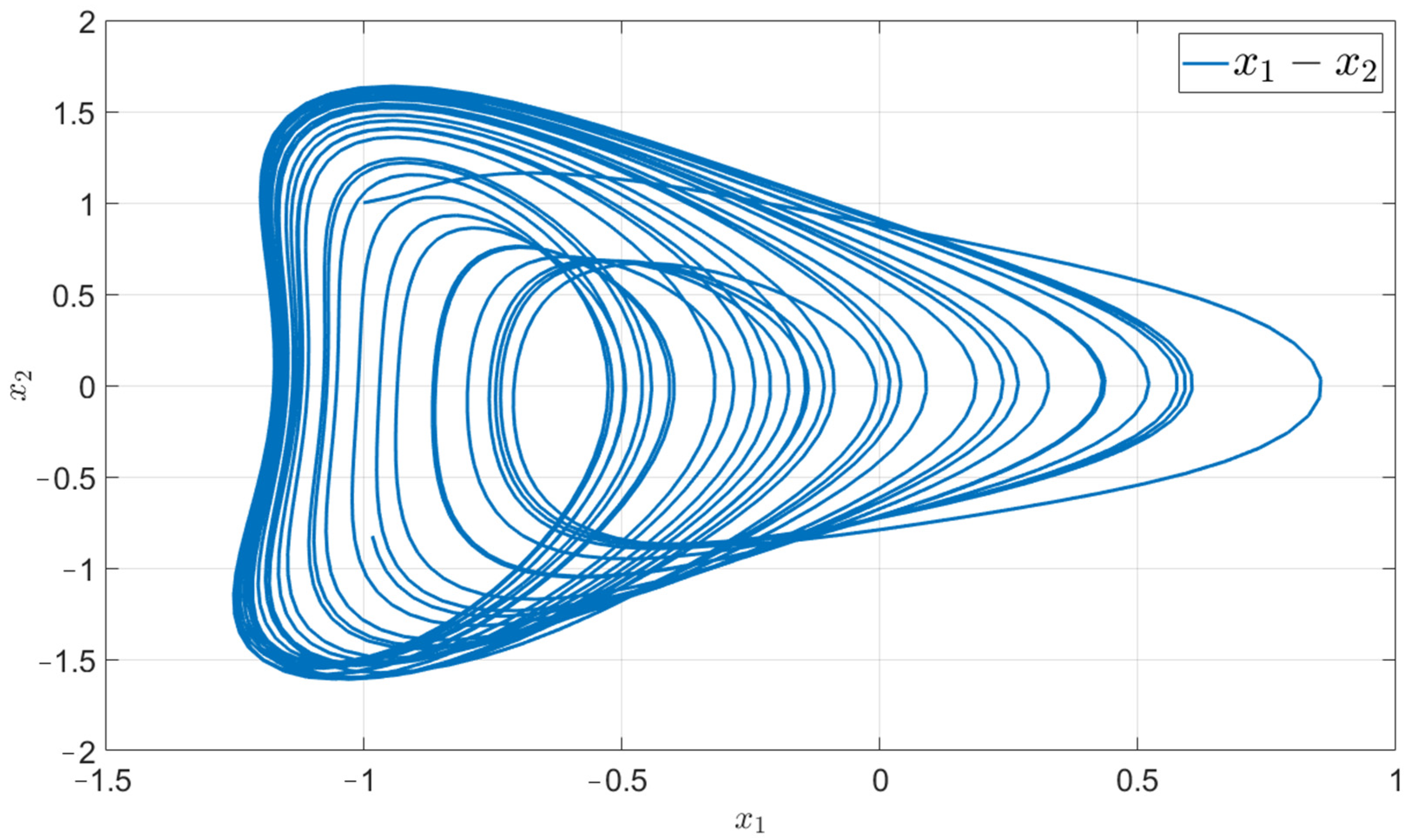
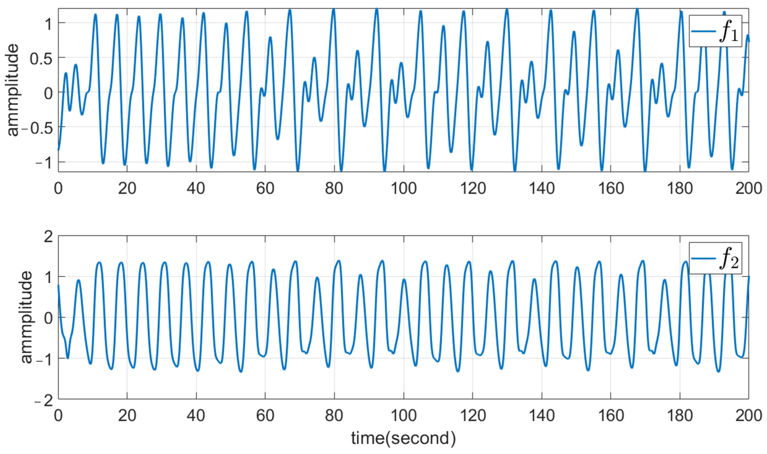
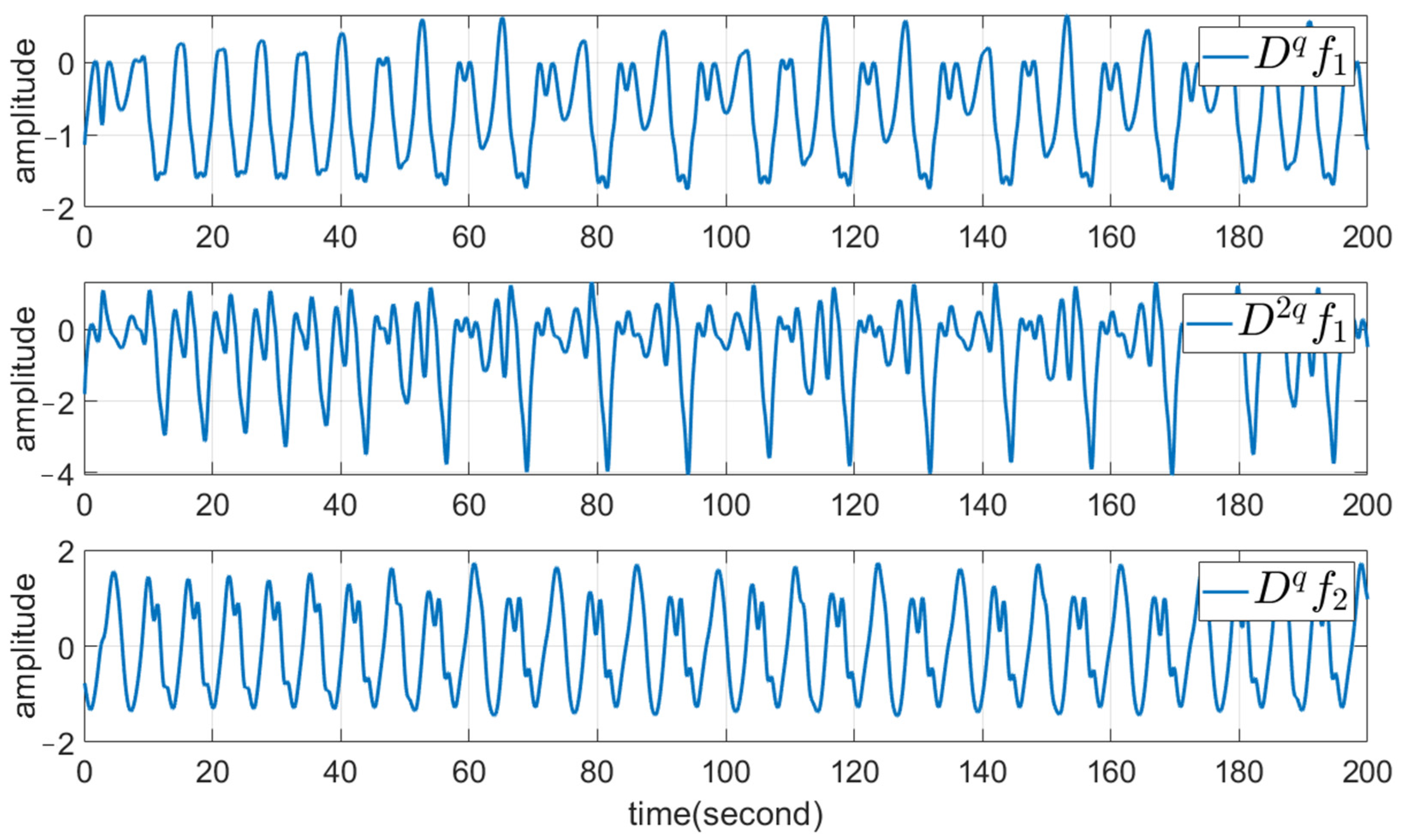
where $\mathrm{x}={[{\mathrm{x}}_1,{\mathrm{x}}_2]}^{\mathrm{T}}$ denotes the accessible system state vector and $\mathrm{y}={\mathrm{x}}_1$ is the system output. With $\mathrm{q}=0.95$ and ${\mathrm{x}}_1(0)=-1$, ${\mathrm{x}}_2(0)=1$, the chaotic behavior is shown in Figure 1. The boundedness of functions ${\mathrm{f}}_1$, ${\mathrm{f}}_2$, ${\Delta }_1$ and ${\Delta }_2$ is shown in Figure 2 and Figure 3 respectively. The parameters of sliding surfaces (8) and (10) are chosen as ${\mathrm{k}}_1=0.5$, ${\mathrm{k}}_2=0.5$, ${\mathrm{k}}_3=1$, ${\mathrm{\lambda }}_1=0.1$, and ${\mathrm{\lambda }}_2=1$. Other design parameters are ${\mathrm{\delta }}_1=2$, ${\mathrm{\delta }}_2=2$, ${\mathrm{\sigma }}_1=0.5$, and ${\mathrm{\sigma }}_2=0.5$; moreover, ${\mathrm{a}}_1=-1$, ${\mathrm{a}}_2=0$, $\mathrm{\mu }=1$, and $\phi =\mathrm{10,000}$. The initial conditions are chosen as ${\mathrm{x}}_1(0)=1$, ${\mathrm{x}}_2(0)=1$ and ${\dot{\mathrm{x}}}_1(0)=0$, ${\ddot{\mathrm{x}}}_1(0)=0$, and ${\dot{\mathrm{x}}}_2(0)=0$. To calculate the derivative of input control signal ${\mathrm{D}}^{\mathrm{q}}\mathrm{u}$, the initial value of $\mathrm{u}$ is needed which is set to zero, i.e., $\mathrm{u}(0)=0$. Simulation was done by MATLAB-R2022a with a fixed step time of 0.001.

Remark 3.

Considering Equations (22) and (29), we have:

$$\sqrt{{\displaystyle \frac{\overline{\mathrm{\sigma }}({\mathrm{P}}_1)}{\phi }}}=0.8527,\sqrt{{\displaystyle \frac{\overline{\mathrm{\sigma }}({\mathrm{P}}_2)}{\phi }}}=0.4057$$

(47)

So, the big value of $\phi =\mathrm{10,000}$ is not very critical in a closed-loop system.

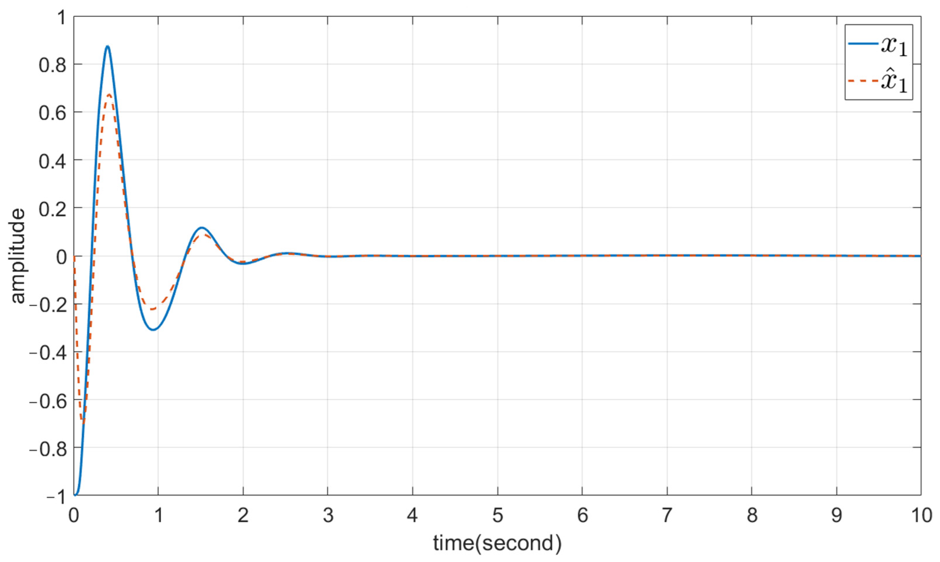
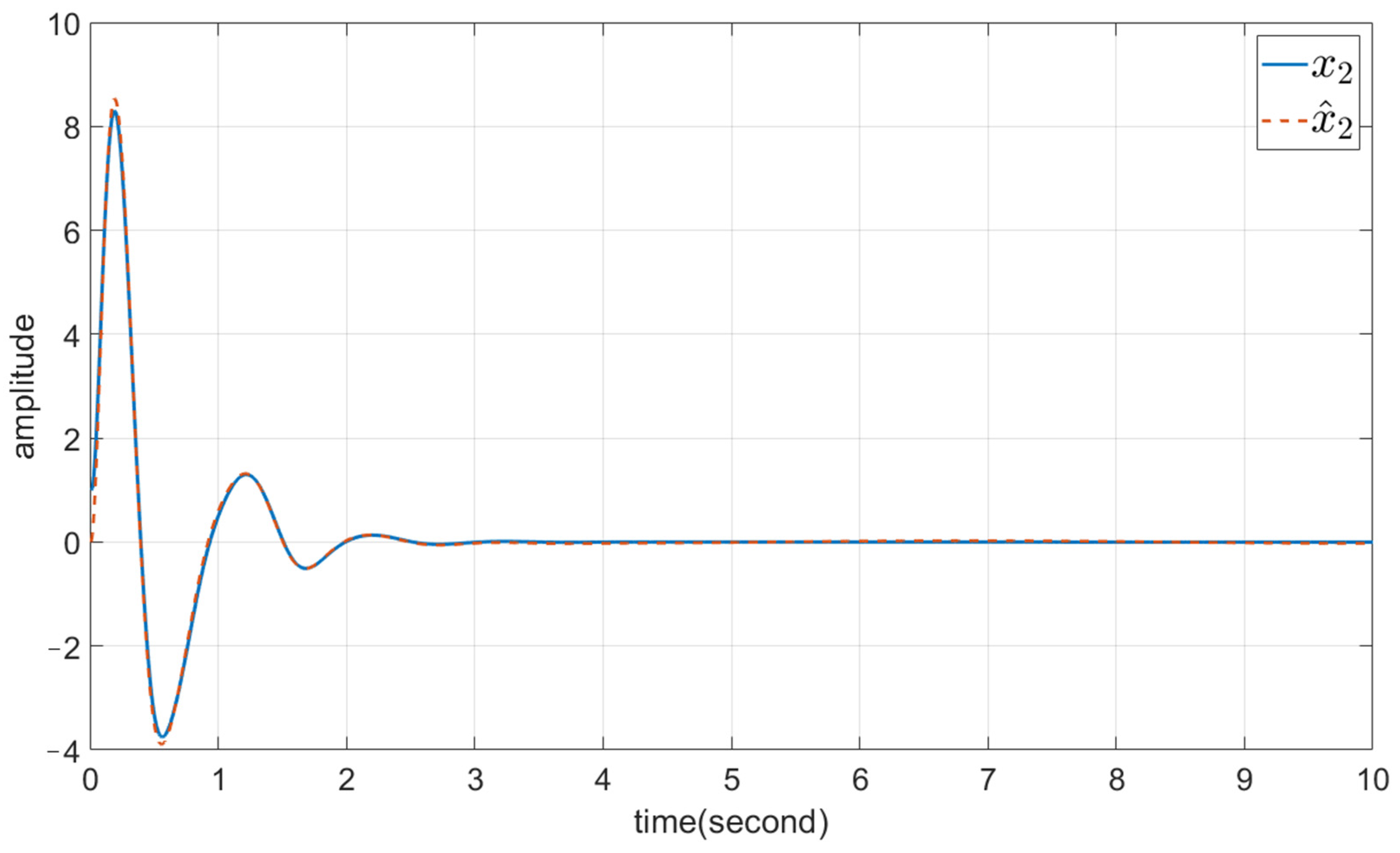
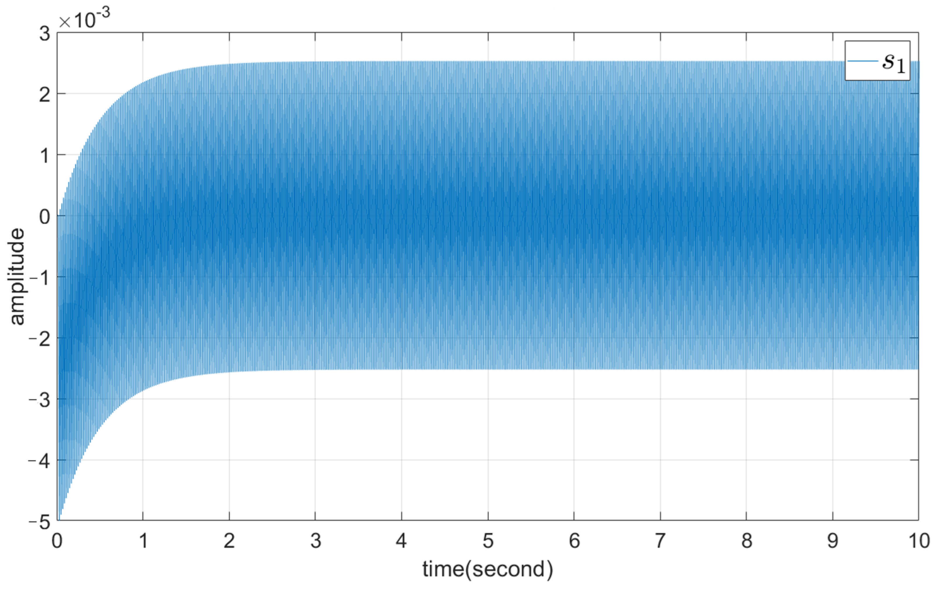
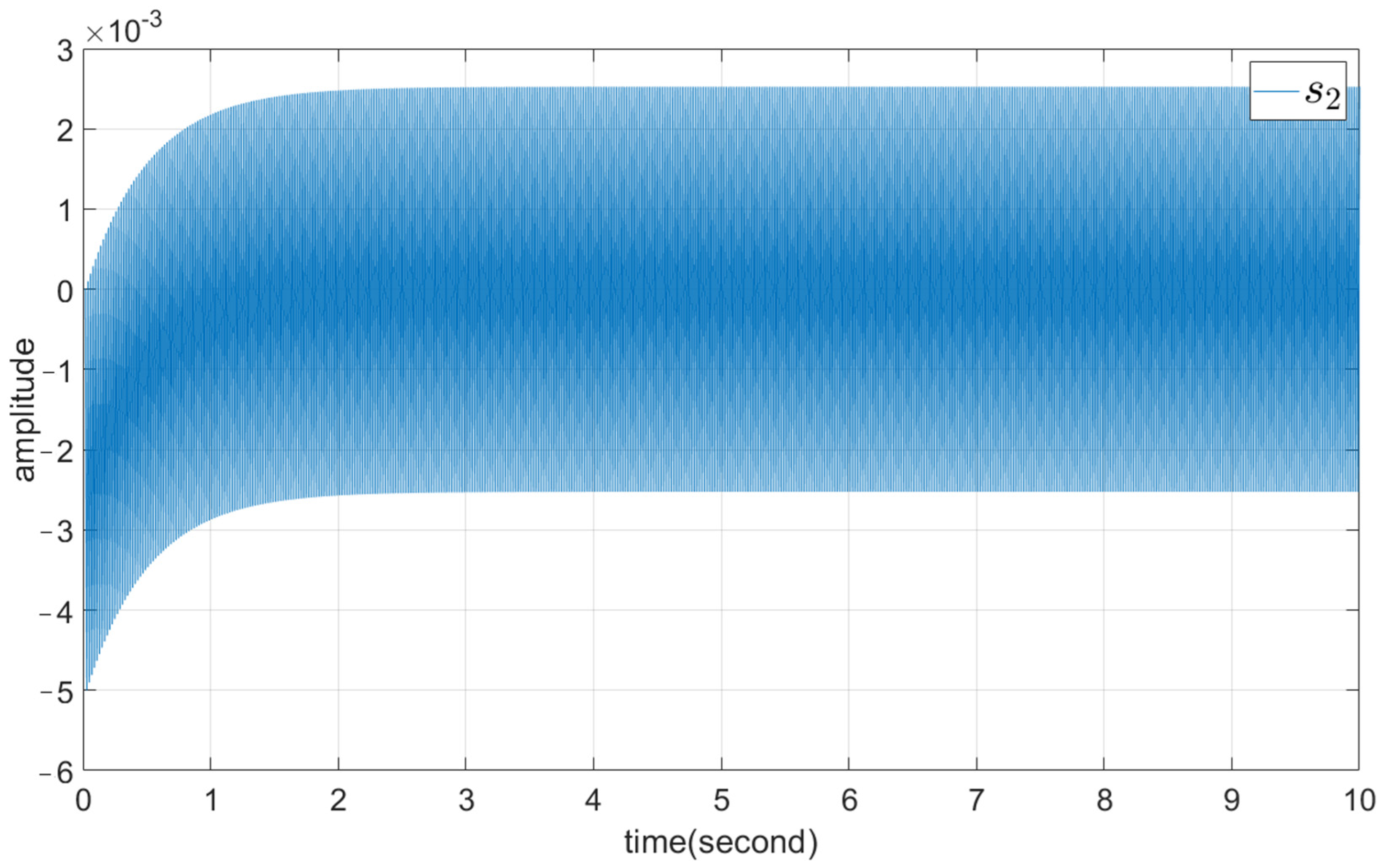
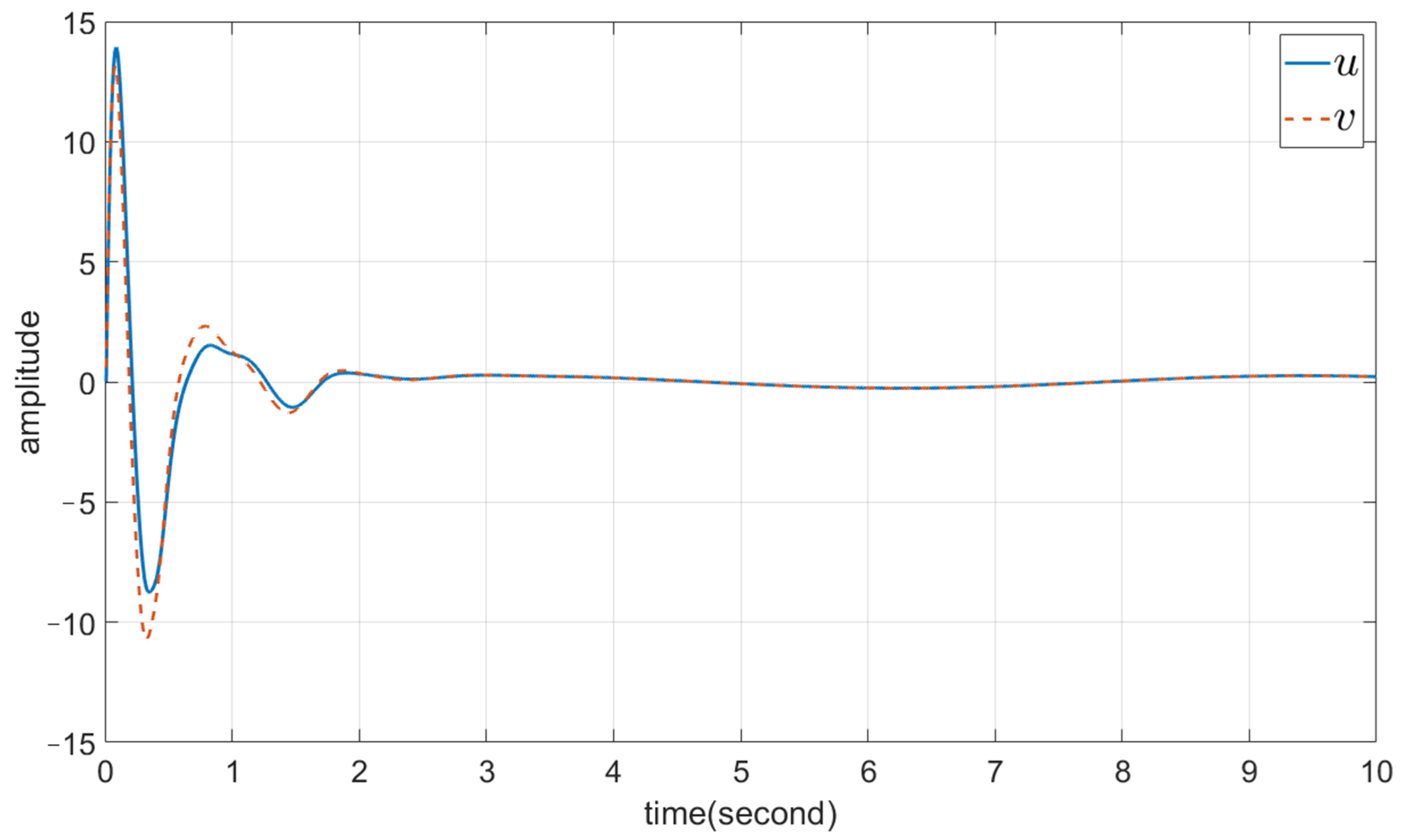
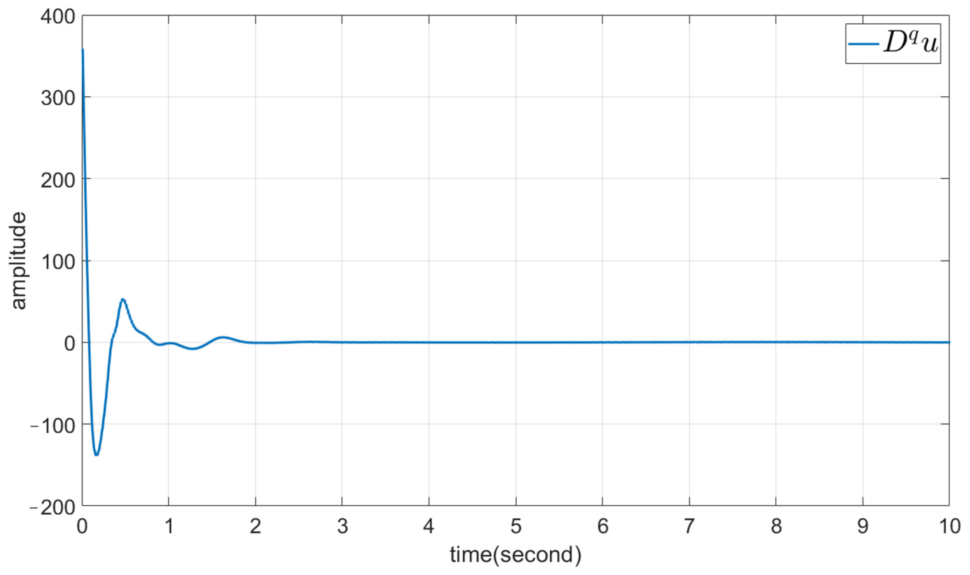
The simulation outcomes are presented in Figure 4, Figure 5, Figure 6, Figure 7, Figure 8 and Figure 9. Figure 4 and Figure 5 illustrate the system states. As shown in Figure 4, the system output converges to zero despite the presence of uncertainties. Figure 6 and Figure 7 display the sliding surfaces, which also converge to zero. The switching amplitude produced by the Sign function remains very small in the vicinity of these surfaces. Figure 8 demonstrates that the system control input $\mathrm{u}$ is smooth and free of switching behavior. Although the initial value of the auxiliary signal ${\mathrm{D}}^{\mathrm{q}}\mathrm{u}$ in Figure 9 is large, it is irrelevant because this signal is not applied directly to the system. Overall, the simulation confirms that the proposed method eliminates chattering while preserving the invariance property for both matched and mismatched uncertainties.

Remark 4.

In the proposed simulation scenario, the entire system dynamics are treated as uncertainties—either matched or mismatched. This can be seen from (13), which covers all the system dynamics as the uncertainty into the variables ${\Delta }_1={\mathrm{D}}^{2\mathrm{q}}{\mathrm{f}}_1(\mathrm{x},\mathrm{t})$ and ${\Delta }_2={\mathrm{a}}_2{\mathrm{D}}^{\mathrm{q}}{\mathrm{f}}_2(\mathrm{x},\mathrm{t})$. In other words, the approach is model-free.

Remark 5.

Refer to Equations (1) and (2); then, the fractional derivative and integration at any given moment depends on the state of the system in the past, that is, the total time since the beginning of the experiment. So, it can be more robust from the ordinary derivative and integration. Therefore, fractional-order systems are useful in studying the anomalous behavior of dynamical systems in physics, electrochemistry, biology, viscoelasticity and chaotic systems.

6. Conclusions

Fractional traditional sliding mode control (FT-SMC) suffers from two main limitations: chattering and sensitivity to mismatched uncertainties. This paper introduces a new method to address both issues for the extended fractional Duffing–Holmes chaotic system (EF-DHCS). The proposed solution employs fractional dynamic sliding mode control (FD-SMC) to regulate the output of nonlinear systems affected by mismatched uncertainties, using a structure based on multiple sliding surfaces. To overcome the challenge of estimating the sliding surface in FD-SMC, a robust optimal fractional loop-transfer-recovery observer (ROF-LTRO) is incorporated. Notably, the design does not require knowledge of the upper bound of uncertainties in either FD-SMC or ROF-LTRO, which is a significant advantage for practical implementation. The proposed method is conceptually straightforward, easy to implement, and completely free of chattering. Moreover, it preserves the invariance property for both matched and mismatched uncertainties.

References

1. Lee, H.; Utkin, V.-I. Chattering suppression methods in sliding mode control systems. Annu. Rev. Control 2007, 31, 179–188. [Google Scholar] [CrossRef]
2. Karami-Mollaee, A.; Pariz, N.; Shanechi, H.M. Position control of servomotors using neural dynamic sliding mode. J. Dyn. Syst. Meas. Control. Trans. ASME 2011, 133, 141–150. [Google Scholar] [CrossRef]
3. Perruquetti, W.; Pierre-Barbot, J. Sliding Mode Control in Engineering; Marcel Dekker: New York, NY, USA, 2002. [Google Scholar]
4. Allamehzadeh, H.; Cheung, J.Y. Optimal fuzzy sliding mode control with adaptive boundary layer. WSEAS Trans. Syst. 2004, 3, 1887–1892. [Google Scholar]
5. Zhang, X. Sliding mode-like fuzzy logic control with adaptive boundary layer for multiple-variable discrete. J. Intell. Syst. 2016, 25, 209–220. [Google Scholar] [CrossRef]
6. Chen, H.-M.; Renn, J.-C.; Su, J.-P. Sliding mode control with varying boundary layers for an electro-hydraulic position servo system. Int. J. Adv. Manuf. Technol. 2005, 26, 117–123. [Google Scholar] [CrossRef]
7. Fuh, C.-C. Variable-thickness boundary layers for sliding mode control. J. Mar. Sci. Technol. 2008, 16, 288–294. [Google Scholar] [CrossRef]
8. Levant, A. Robust exact differentiation via sliding mode techniques. Automatica 1998, 34, 379–384. [Google Scholar] [CrossRef]
9. Karami-Mollaee, A.; Barambones, O. Higher order sliding mode control of MIMO induction motors: A new adaptive approach. Mathematics 2023, 11, 4558. [Google Scholar] [CrossRef]
10. Zhu, Q.; Zhang, J.; Liu, Z.; Yu, S. Robust higher-order nonsingular terminal sliding mode control of unknown nonlinear dynamic systems. Mathematics 2025, 13, 1559. [Google Scholar] [CrossRef]
11. Bartolini, G.; Ferrara, A.; Usai, E. Chattering avoidance by second-order sliding mode control. IEEE Trans. Autom. Control 1998, 43, 241–246. [Google Scholar] [CrossRef]
12. Kchaou, A.; Naamane, A.; Koubaa, Y.; M’sirdi, N. Second order sliding mode-based MPPT control for photovoltaic applications. Sol. Energy 2017, 155, 758–769. [Google Scholar] [CrossRef]
13. Cao, T.N.T.; Pham, B.T.; Nguyen, N.T.; Vu, D.-L.; Truong, N.-V. Second-order terminal sliding mode control for trajectory tracking of a differential drive robot. Mathematics 2024, 12, 2657. [Google Scholar] [CrossRef]
14. Chen, M.-S.; Chen, C.-H.; Yang, F.-Y. An LTR-observer based dynamic sliding mode control for chattering reduction. Automatica 2007, 43, 1111–1116. [Google Scholar] [CrossRef]
15. Karami-Mollaee, A. Design of dynamic sliding mode controller for active suspension system. Modares Mech. Eng. 2016, 16, 51–58. [Google Scholar]
16. Karami-Mollaee, A.; Tirandaz, H. Adaptive fuzzy fault tolerant control using dynamic sliding mode. Int. J. Control Autom. Syst. 2018, 16, 360–367. [Google Scholar] [CrossRef]
17. Karami-Mollaee, A.; Tirandaz, H. Estimation of load torque in induction motors via dynamic sliding mode control and new nonlinear state observer. J. Mech. Sci. Technol. 2018, 32, 2283–2288. [Google Scholar] [CrossRef]
18. Karami-Mollaee, A.; Shojaei, A.A.; Barambones, O.; Fauzi, O. Dynamic sliding mode control of pitch blade wind turbine using sliding mode observer. Trans. Inst. Meas. Control 2022, 44, 3028–3038. [Google Scholar] [CrossRef]
19. Karami-Mollaee, A.; Barambones, O. On neural observer in dynamic sliding mode control of permanent magnet synchronous wind generator. Mathematics 2024, 12, 2246. [Google Scholar] [CrossRef]
20. Ding, Q.; Chen, H.; Jiang, C.; Chen, Z. Combined indirect and direct method for adaptive fuzzy output feedback control of nonlinear system. J. Syst. Eng. Electron. 2007, 18, 120–124. [Google Scholar] [CrossRef]
21. Slotine, J.J.E.; Li, W. Applied Nonlinear Control; Prentice Hall: Englewood Cliffs, NJ, USA, 1991. [Google Scholar]
22. Chan, M.-L.; Tao, C.W.; Lee, T.-T. Sliding mode controller for linear systems with mismatched time-varying uncertainties. J. Frankl. Inst. 2000, 337, 105–115. [Google Scholar] [CrossRef]
23. Choi, H.H. LMI-based sliding surface design for integral sliding mode control of mismatched uncertain systems. IEEE Trans. Autom. Control 2007, 52, 736–742. [Google Scholar] [CrossRef]
24. Wen, C.-C.; Cheng, C.-C. Design of sliding surface for mismatched uncertain systems to achieve asymptotical stability. J. Frankl. Inst. 2008, 345, 926–941. [Google Scholar] [CrossRef]
25. Wang, Y.; Jiang, C.; Zhou, D.; Gao, F. Variable structure control for a class of nonlinear systems with mismatched uncertainties. Appl. Math. Comput. 2008, 200, 387–400. [Google Scholar] [CrossRef]
26. Yang, J.; Li, S.; Yu, X. Sliding-mode control for systems with mismatched uncertainties via a disturbance observer. IEEE Trans. Ind. Electron. 2013, 60, 160–169. [Google Scholar] [CrossRef]
27. Yang, J.; Li, S.; Su, J.; Yu, X. Continuous nonsingular terminal sliding mode control for systems with mismatched disturbances. Automatica 2013, 49, 2287–2291. [Google Scholar] [CrossRef]
28. Ginoya, D.; Shendge, P.D.; Phadke, S.B. Sliding mode control for mismatched uncertain systems using an extended disturbance observer. IEEE Trans. Ind. Electron. 2014, 61, 1983–1992. [Google Scholar] [CrossRef]
29. Yang, J.; Su., J.; Li, S.; Yu, X. High-order mismatched disturbance compensation for motion control systems via a continuous dynamic sliding-mode approach. IEEE Trans. Ind. Inform. 2014, 10, 604–614. [Google Scholar] [CrossRef]
30. Ginoya, D.; Shendge, P.D.; Phadke, S.B. Disturbance observer based sliding mode control of nonlinear mismatched uncertain systems. Commun. Nonlinear Sci. Numer. Simul. 2015, 26, 98–107. [Google Scholar] [CrossRef]
31. Fanbiao, L.; Ligang, W.; Peng, S.; Cheng-Chew, L. State estimation and sliding mode control for semi-Markovian jump systems with mismatched uncertainties. Automatica 2015, 51, 385–393. [Google Scholar] [CrossRef]
32. Zhang, Y.; Li, R.; Xue, T.; Lei, Z. Exponential sliding mode tracking control via back-stepping approach for a hypersonic vehicle with mismatched uncertainty. J. Frankl. Inst. 2016, 353, 2319–2343. [Google Scholar] [CrossRef]
33. Zheng, B.-C.; Park, J.H. Sliding mode control design for linear systems subject to quantization parameter mismatch. J. Frankl. Inst. 2016, 353, 37–53. [Google Scholar] [CrossRef]
34. Shyu, K.-K.; Tsai, Y.-W.; Lai, C.-K. A dynamic output feedback controllers for mismatched uncertain variable structure systems. Automatica 2001, 37, 775–779. [Google Scholar] [CrossRef]
35. Yan, X.-G.; Spurgeon, S.K.; Edwards, C. Dynamic sliding mode control for a class of systems with mismatched uncertainty. Eur. J. Control 2005, 11, 1–10. [Google Scholar] [CrossRef]
36. Xiang, W.; Chen, F. An adaptive sliding mode control scheme for a class of chaotic systems with mismatched perturbations and input nonlinearities. Commun. Nonlinear Sci. Numer. Simul. 2001, 16, 1–9. [Google Scholar] [CrossRef]
37. Mondal, S.; Mahanta, C. Chattering free adaptive multivariable sliding mode controller for systems with matched and mismatched uncertainty. ISA Trans. 2013, 52, 335–341. [Google Scholar] [CrossRef] [PubMed]
38. Polyakov, A.; Poznyak, A. Invariant ellipsoid method for minimization of unmatched disturbances effects in sliding mode control. Automatica 2011, 47, 1450–1454. [Google Scholar] [CrossRef]
39. Huang, A.-C.; Chen, Y.-C. Adaptive multiple-surface sliding control for non-autonomous systems with mismatched uncertainties. Automatica 2004, 40, 1939–1945. [Google Scholar] [CrossRef]
40. Tsai, Y.-C.; Huang, A.-C. FAT-based adaptive control for pneumatic servo systems with mismatched uncertainties. Mech. Syst. Signal Process. 2008, 22, 1263–1273. [Google Scholar] [CrossRef]
41. You, L.; Li, X. Observer-based sliding mode control of impulsive systems with unknown mismatched disturbances. Expert Syst. Appl. 2025, 276, 127092. [Google Scholar] [CrossRef]
42. Dong, H.; Yang, X.; Kuang, Z.; Liu, M. On practical terminal sliding-mode control for system with or without mismatched uncertainty. J. Frankl. Inst. 2022, 359, 8084–8106. [Google Scholar] [CrossRef]
43. Moulay, E.; Lechappe, V.; Bernuau, E.; Defoort, M.; Plestan, F. Fixed-time sliding-mode control with mismatched disturbances. Automatica 2022, 136, 110009. [Google Scholar] [CrossRef]
44. Thanh, H.L.N.N.; Hong, S.K. An extended multi-surface sliding control for matched/mismatched uncertain nonlinear systems through a lumped disturbance estimator. IEEE Access 2020, 8, 91468–91475. [Google Scholar] [CrossRef]
45. Hou, L.; Li, W.; Shen, H.; Li, T. Fuzzy sliding mode control for systems with matched and mismatched uncertainties/disturbances based on ENDOB. IEEE Access 2018, 7, 666–673. [Google Scholar] [CrossRef]
46. Min, W.; Liu, Q. An improved adaptive fuzzy backstepping control for nonlinear mechanical systems with mismatched uncertainties. Automatika 2019, 60, 1–10. [Google Scholar] [CrossRef]
47. Ivo, P. Fractional Order Nonlinear Systems; Springer: Berlin/Heidelberg, Germany, 2011. [Google Scholar]
48. Kilbsa, A.A.; Srivastava, H.M.; Trujillo, J.J. Theory and Applications of Fractional Differential Equations; Elsevier: New York, NY, USA, 2006; Volume 204. [Google Scholar]
49. Podlubny, I. Fractional Differential Equations: An Introduction to Fractional Derivatives, Fractional Differential Equations, to Methods of Their Solution and Some of Their Applications; Academic Press: San Diego, DC, USA, 1998; Volume 198. [Google Scholar]
50. Rapaić, M.R.; Jeličić, Z.D. Optimal control of a class of fractional heat diffusion systems. Nonlinear Dyn. 2010, 62, 39–51. [Google Scholar] [CrossRef]
51. Aguila-Camacho, N.; Duarte-Mermoud, M.A.; Gallegos, J.A. Lyapunov functions for fractional order systems. Commun. Nonlinear Sci. Numer. Simul. 2014, 19, 2951–2957. [Google Scholar] [CrossRef]
52. Li, Y.; Chen, Y.; Podlubny, I. Stability of fractional-order nonlinear dynamic systems: Lyapunov direct method and generalized Mittag Leffler stability. Comput. Math. Appl. 2010, 59, 181021. [Google Scholar] [CrossRef]
53. Shantanu, D. Functional Fractional Calculus for System Identification and Controls; Springer: Berlin/Heidelberg, Germany, 2008. [Google Scholar]
54. Efe, M.Ö.; Kasnakoglu, C. A fractional adaptation law for sliding mode control. Int. J. Adapt. Control Signal Process. 2008, 22, 968–986. [Google Scholar] [CrossRef]
55. Muoz-Vzquez, A.J.; Parra-Vega, V.; Snchez-Orta, A. Fractional integral sliding modes for robust tracking of nonlinear systems. Nonlinear Dyn. 2017, 87, 895–901. [Google Scholar] [CrossRef]
56. Ni, J.; Liu, L.; Liu, C.; Hu, X. Fractional order fixed-time nonsingular terminal sliding mode synchronization and control of fractional order chaotic systems. Nonlinear Dyn. 2017, 89, 2065–2083. [Google Scholar] [CrossRef]
57. Jakovljević, B.; Pisano, A.; Rapaić, M.R.; Usai, E. On the sliding-mode control of fractional-order nonlinear uncertain dynamics. Int. J. Robust Nonlinear Control 2016, 26, 782–798. [Google Scholar] [CrossRef]
58. Bettayeb, M.; Djennoune, S. Design of sliding mode controllers for nonlinear fractional-order systems via diffusive representation. Nonlinear Dyn. 2016, 84, 593–605. [Google Scholar] [CrossRef]
59. Dadras, S.; Momeni, H.R. Fractional-order dynamic output feedback sliding mode control design for robust stabilization of uncertain fractional-order nonlinear systems. Asian J. Control 2014, 16, 489–497. [Google Scholar] [CrossRef]
60. Zhang, D.; Cao, L.; Tang, S. Fractional-order sliding mode control for a class of uncertain nonlinear systems based on LQR. Int. J. Adv. Robot. Syst. 2017, 14, 1729881417694290. [Google Scholar] [CrossRef]
61. Liu, Y.-T.; Kung, T.-T.; Chang, K.-M.; Chen, S.-Y. Observer-based adaptive sliding mode control for pneumatic servo system. Precis. Eng. 2013, 37, 522–530. [Google Scholar] [CrossRef]
62. Xia, Y.; Zhu, Z.; Fu, M. Back-stepping sliding mode control for missile systems based on an extended state observer. IET Control Theory Appl. 2011, 5, 93–102. [Google Scholar] [CrossRef]
63. Fuyang, C.; Lei, W.; Zhang, K.; Tao, G.; Jiang, B. A novel nonlinear resilient control for a quadrotor UAV via backstepping control and nonlinear disturbance observer. Nonlinear Dyn. 2016, 85, 1281–1295. [Google Scholar] [CrossRef]
64. Butt, Q.R.; Bhatti, A.I.; Mufti, M.R.; Rizvi, M.A.; Awan, I. Modeling and online parameter estimation of intake manifold in gasoline engines using sliding mode observer. Simul. Model. Pract. Theory 2013, 32, 138–154. [Google Scholar] [CrossRef]
65. Davila, J.; Fridman, L.; Levant, A. Second-order sliding mode observer for mechanical systems. IEEE Trans. Autom. Control 2005, 50, 1785–1789. [Google Scholar] [CrossRef]
66. Xiong, Y.; Saif, M. Sliding mode observer for nonlinear uncertain systems. IEEE Trans. Autom. Control 2001, 46, 2012–2017. [Google Scholar] [CrossRef]
67. Benchaib, A.; Rachid, A.; Audrezet, E.; Tadjine, M. Real time sliding-mode observer and control of an induction motor. IEEE Trans. Ind. Electron. 1999, 46, 128–138. [Google Scholar] [CrossRef]
68. Doyle, J.C.; Stein, G. Robustness with observers. IEEE Trans. Autom. Control 1979, 24, 607–611. [Google Scholar] [CrossRef]
Figure 1. Chaotic behavior of system.
Mathematics 14 02130 g001
Figure 2. Time series of functions f 1 and f 2 .
Mathematics 14 02130 g002
Figure 3. Time series of functions Δ 1 and Δ 2
Mathematics 14 02130 g003
Figure 4. First state and its estimation.
Mathematics 14 02130 g004
Figure 5. Second state and its estimation.
Mathematics 14 02130 g005
Figure 6. First sliding surface.
Mathematics 14 02130 g006
Figure 7. Second sliding surface.
Mathematics 14 02130 g007
Figure 8. Input control signals.
Mathematics 14 02130 g008
Figure 9. Fractional derivative of input control signal (auxiliary signal).
Mathematics 14 02130 g009
Disclaimer/Publisher’s Note: The statements, opinions and data contained in all publications are solely those of the individual author(s) and contributor(s) and not of MDPI and/or the editor(s). MDPI and/or the editor(s) disclaim responsibility for any injury to people or property resulting from any ideas, methods, instructions or products referred to in the content.