ISS in Different Norms of Coupled Nonlinear Parabolic PDEs with Dirichlet Boundary Disturbances

Abstract

This paper addresses the input-to-state stability (ISS) in different $L^q$-norms for a class of coupled nonlinear partial differential equations of parabolic type subject to both in-domain disturbances and Dirichlet boundary disturbances, where $q\in [1,+\infty )$. Specifically, we first prove the continuous dependence of solutions to the system on initial data and disturbances in different $L^q$-norms by using the generalized Lyapunov method, and subsequently derive ISS estimates via a density argument. The main challenge arises in handling the nonlinear coupling terms and deriving ISS small-gain conditions within the generalized Lyapunov framework, as each coupling term depends on all other state variables of the system.

1. Introduction

Over the past decade, extensive research efforts have been devoted to the development of input-to-state stability (ISS) theory for infinite-dimensional systems governed by partial differential equations (PDEs) [1,2,3,4,5]. It is widely known that the Lyapunov method is commonly employed for stability analysis. While employing this method to ISS for parabolic PDEs with in-domain disturbances and Robin or Neumann boundary disturbances does not present essential difficulties, applying it to PDEs with Dirichlet boundary disturbances is fraught with challenges, as demonstrated in [1].

To overcome the difficulties posed by Dirichlet boundary disturbances, most existing literature proposes the establishment of ISS for PDEs with Dirichlet boundary disturbances via non-Lyapunov methods, as summarized in [6]. However, these non-Lyapunov methods often lack universality and are difficult to generalize to a broader class of PDEs. Given that the Lyapunov method is a fundamental tool for stability analysis and is generally easier to implement compared to non-Lyapunov approaches, exploring how to employ the Lyapunov method to establish the ISS for PDEs with Dirichlet boundary disturbances is of significant theoretical and practical importance.

Within the framework of Lyapunov stability, a novel method, namely the generalized Lyapunov method, was adopted to establish the global ISS estimates in various norms for the viscous Burgers’ equation with Dirichlet boundary disturbances [7]. The key to this method lies in constructing a generalized Lyapunov functional (GLF) based on Stampacchia’s truncation techniques and the approximations of Lyapunov functionals. Compared with classical Lyapunov functionals, the GLF has two distinctive features: it can be positive semi-definite and its formulation may depend on disturbances. These features enable more flexible selection of Lyapunov candidates for PDEs with Dirichlet boundary disturbances, providing a new perspective for ISS analysis of PDEs.

Building upon this foundation, the generalized Lyapunov method was further applied to the ISS assessment of two classes of PDEs: parabolic equations with Dirichlet boundary disturbances and coupled parabolic equations with only distributed in-domain disturbances [8]. Notably, the generalized Lyapunov method enables ISS analysis for parabolic PDEs with variable coefficients and Dirichlet boundary disturbances. Moreover, the method has also been applied to investigate the stabilization problem for a class of parabolic PDEs with Dirichlet and Robin boundary disturbances, establishing ISS in the $L^{\infty }$-norm for the closed-loop system under output feedback control [9]. Nevertheless, applying the generalized Lyapunov method to coupled parabolic PDEs with Dirichlet boundary disturbances deserves in-depth investigation, which motivates the work of this paper.

Another motivation of this research stems from the broad prospects demonstrated by coupled parabolic PDEs in various scientific and engineering fields, which provide a modeling framework for multi-agent systems, networked distributed parameter systems, neural networks, etc. For instance, in multi-agent systems, this model has been utilized to achieve cooperative output regulation [10], flatness-based motion planning [11], and consensus control in diffusion networks [12]; in the cooperative control of networked distributed parameter systems, it has been applied to address problems such as leader–follower synchronization [13] and synchronization controller design based on active disturbance rejection control [14]; in the field of neural networks, this framework also provides a theoretical basis for analyzing issues such as global exponential stability [15,16], impulsive synchronization [17], and adaptive synchronization [18] in reaction–diffusion neural networks. These studies demonstrate the powerful capability of coupled PDEs in modeling and analyzing complex spatiotemporal dynamic behaviors. Considering the aforementioned wide-ranging applications, it is of great significance to establish the stability of coupled parabolic PDEs with Dirichlet boundary disturbances.

It is worth mentioning that the continuous dependence of solutions of PDEs on initial data and disturbances is not only significant in the development of regularity theory but also plays a key role in the ISS analysis of the system [19]. Theoretically, the continuous dependence of solutions enables the extension of ISS properties from dense subspaces to the entire state spaces (Lemma 1.4.2, p. 25 in [19]). This allows us to establish the ISS estimates by using the technique of approximation and Lyapunov or non-Lyapunov methods within the framework of either classical or weak solutions. Notably, in [20], the continuous dependence in the $L^{\infty }$-norm was established for weak solutions of nonlinear parabolic equations with Robin boundary conditions by using the De Giorgi iteration method. Then, this result was used to derive small-gain conditions that ensure the ISS in the $L^{\infty }$-norm for a class of cascaded nonlinear parabolic PDEs [20].

Following these developments, the aim of this paper is to establish the ISS estimates for a class of coupled nonlinear parabolic PDEs with Dirichlet boundary disturbances, based on the application of the generalized Lyapunov method. Specifically, we first prove the continuous dependence of solutions on initial data and disturbances in different $L^q$-norms with $q\in [1,+\infty )$, and then, by combining a density argument, also establish ISS estimates in the $L^q$-norms for the system.

Compared with existing literature, the main contributions of this paper are twofold:

(i)

Coupled nonlinear PDEs composed of n components are considered, in which each coupling term depends on all other state variables of the system except its corresponding component, and small-gain conditions ensuring the ISS property of the system are provided.

(ii)

The effects of both in-domain disturbances and Dirichlet boundary disturbances are addressed simultaneously, and explicit ISS estimates for the system are obtained in different $L^q$-norms with $q\in [1,+\infty )$.

In the rest of this paper, we first introduce some basic notations. Section 2 presents the problem setting, main results, and methodology; Section 2.1 provides the problem formulation and related definitions; Section 2.2 presents the properties of the continuous dependence of solutions on initial data and disturbances and the main results on the ISS in different norms; Section 2.3 introduces the main idea of the generalized Lyapunov method used for stability analysis, as well as some technical lemmas. Section 3 is devoted to the proofs of main results: we first employ the generalized Lyapunov method to establish the continuous dependence and then, by combining this result with a density argument, derive the ISS estimates. The proofs are organized into three subsections according to the range of q: Section 3.1 provides a proof for some $q\in [2,+\infty )$ satisfying a certain condition; Section 3.2 provides a proof for all $q\in [2,+\infty )$; and Section 3.3 provides a proof for all $q\in [1,2]$. In each subsection, both the continuous dependence and the ISS estimate are proved in the corresponding $L^q$-norm. Numerical simulations are provided in Section 4 to illustrate the ISS property for coupled nonlinear parabolic PDEs with Dirichlet boundary disturbances. Concluding remarks are provided in Section 5.

Notation. Let $\mathbb{R}:=\left(-\infty ,+\infty \right)$, ${\mathbb{R}}_{>0}:=\left(0,+\infty \right)$, ${\mathbb{R}}_{\ge 0}:=\left[0,+\infty \right)$, and ${\mathbb{R}}_{\le 0}:=\left(-\infty ,0\right]$.

For $q\in \left[1,+\infty \right)$ and an arbitrary open or closed domain $\Omega$ in ${\mathbb{R}}^1$ or ${\mathbb{R}}^2$, the notation of $L^q\left(\Omega \right)$ denotes the standard Lebesgue spaces with elements defined over $\Omega$. The norms of a function u in $L^q\left(0,1\right)$ with $q\in \left[1,+\infty \right)$ and $L^{\infty }\left(0,1\right)$ are defined as ${\parallel u\parallel }_{L^q\left(0,1\right)}:={\left({\int }_0^1{\left|u\left(x\right)\right|}^q\mathrm{d}x\right)}^{{\displaystyle \frac{1}{q}}}$ and ${\parallel u\parallel }_{L^{\infty }\left(0,1\right)}:=\mathrm{ess}{\sup }_{x\in \left(0,1\right)}\left|u\left(x\right)\right|$, respectively. For any $T\in {\mathbb{R}}_{>0}$, let $Q_T:=\left(0,1\right)\times \left(0,T\right)$ and ${\overline{Q}}_T:=[0,1]\times [0,T]$. Let $Q_{\infty }:=\left(0,1\right)\times {\mathbb{R}}_{>0}$ and ${\overline{Q}}_{\infty }:=[0,1]\times {\mathbb{R}}_{\ge 0}$. The norms of a function u in $L^{\infty }\left(0,T\right)$ and $L^{\infty }\left(Q_T\right)$ are defined as $L^{\infty }\left(0,T\right):=\mathrm{ess}{\sup }_{t\in \left(0,T\right)}\left|u\left(t\right)\right|$ and ${\parallel u\parallel }_{L^{\infty }\left(Q_T\right)}:=\mathrm{ess}{\sup }_{\left(x,t\right)\in Q_T}\left|u\left(x,t\right)\right|$, respectively. Let $C\left(\Omega \right):=\{v:\Omega \to \mathbb{R}|v$ is continuous on $\Omega \}$, $C^{2,1}\left({\overline{Q}}_T\right):=\{v:{\overline{Q}}_T\to \mathbb{R}|v,v_z,$$v_{zz},v_t\in C\left({\overline{Q}}_T\right)\}$, and $C^{\infty }\left(Q_T\right):=\{v:Q_T\to \mathbb{R}|v$ is infinitely differentiable on $Q_T\}$. For $l\in {\mathbb{R}}_{>0}$, the notations of Hölder spaces ${\mathcal{H}}^l\left({\mathbb{R}}_{\ge 0}\right),{\mathcal{H}}^l\left(\left[0,1\right]\right),{\mathcal{H}}^{l,{\displaystyle \frac{l}{2}}}\left({\overline{Q}}_{\infty }\right),{\mathcal{H}}^{l,{\displaystyle \frac{l}{2}}}\left(Q_T\right)$ used in this paper are adopted from Chapter I of [21]. For $T\in {\mathbb{R}}_{>0}$, and $q\in [1,+\infty )$, let $C\left([0,T];L^q(0,1)\right)$ be the space of continuous functions from $[0,T]$ to $L^q(0,1)$.

Let $\mathcal{K}:=\{\gamma :{\mathbb{R}}_{\ge 0}\to {\mathbb{R}}_{\ge 0}|\gamma \left(0\right)=0,\gamma$ is continuous, strictly increasing}, ${\mathcal{K}}_{\infty }:=\{\gamma \in \mathcal{K}:\gamma$ is unbounded}, $\mathcal{L}:=\{\gamma :{\mathbb{R}}_{\ge 0}\to {\mathbb{R}}_{\ge 0}|\gamma$ is continuous, strictly decreasing, ${lim}_{s\to \infty }\gamma \left(s\right)=0\}$, $\mathcal{KL}:=\{\beta :{\mathbb{R}}_{\ge 0}\times {\mathbb{R}}_{\ge 0}\to {\mathbb{R}}_{\ge 0}|\beta$ is continuous, $\beta \left(·,t\right)\in \mathcal{K},\forall t\in {\mathbb{R}}_{\ge 0}$, and $\beta \left(s,·\right)\in \mathcal{L},\forall s\in {\mathbb{R}}_{>0}\}$.

2. Problem Setting, Main Results, and Methodology

In this section, we state the problem setting and main results, followed by an introduction to the generalized Lyapunov method employed in the ISS analysis, as well as two classical inequalities.

2.1. Problem Setting

We consider a class of coupled nonlinear parabolic PDEs with Dirichlet boundary disturbances:

$${\displaystyle \frac{\partial v_i}{\partial t}}\left(x,t\right)=a_i{\displaystyle \frac{{\partial }^2{v}_i}{\partial x^2}}\left(x,t\right)-b_i{v}_i\left(x,t\right)+h_i\left(\widehat{{\mathbf{v}}_{\mathbf{i}}}\left(x,t\right)\right)+f_i\left(x,t\right),\left(x,t\right)\in Q_{\infty },$$

(1a)

$$v_i\left(0,t\right)=d_i\left(t\right),t\in {\mathbb{R}}_{>0},$$

(1b)

$$v_i\left(1,t\right)=g_i\left(t\right),t\in {\mathbb{R}}_{>0},$$

(1c)

$$v_i\left(x,0\right)=v_{0i}\left(x\right),x\in \left(0,1\right),$$

(1d)

where $i=1,2,\dots ,n$ with $n\ge 2$, $a_i$ and $b_i$ are positive constants, and the functions $h_i:{\mathbb{R}}^{n-1}\to \mathbb{R}$ satisfy

$$\{\begin{array}{c}{h}_i\left(0\right)=0,\hfill \\ |h_i\left(s\right)-h_i\left(\tau \right)|\le L_i|s-\tau |,\forall s,\tau \in {\mathbb{R}}^{n-1},\hfill \end{array}$$

(2)

where $L_i$ are positive constants, the functions $f_i\left(x,t\right)$ represent in-domain disturbances, $d_i\left(t\right)$ and $g_i\left(t\right)(i=1,2,\dots ,n)$ represent Dirichlet boundary disturbances, $\mathbf{v}:=\left(v_i\right):=\left(v_1,v_2,\dots ,v_n\right)$ represents the state with $\widehat{{\mathbf{v}}_{\mathbf{i}}}:=(v_1,v_2,\dots ,v_{i-1},v_{i+1},\dots ,v_n)$, and ${\mathbf{v}}_0:=\left(v_{0i}\right):=\left(v_{01},v_{02},\dots ,v_{0n}\right)$ is the given initial data.

Throughout this paper, without special statements, we always assume that for all $T\in {\mathbb{R}}_{>0}$,

$$\begin{array}{c}\hfill f_i\in L^{\infty }\left({\overline{Q}}_T\right),d_i,g_i\in L^{\infty }\left(0,T\right),v_{0i}\in L^{\infty }\left(0,1\right),i=1,2,\cdots ,n.\end{array}$$

(3)

Now, we present the definitions of a classical solution and a generalized solution for system (1).

Definition 1.

A vector function $\mathbf{v}:=\left(v_i\right)$ is called a classical solution of system (1) if for each i, $v_i\in C^{2,1}\left({\overline{Q}}_T\right)$ with any $T\in {\mathbb{R}}_{>0}$ and Equation (1) is satisfied pointwise.

For any $T\in {\mathbb{R}}_{>0}$, multiplying both sides of Equation (1a) by an arbitrary smooth function $\eta (x,t)$, integrating over the domain $Q_T$ and applying integration by parts leads to the following definition of a generalized solution for the system.

Definition 2.

Let $q\in [1,+\infty )$. A vector function $\mathbf{v}:=\left(v_i\right)$ is called a generalized solution of system (1) if for each i, $v_i\in C\left([0,T];L^q(0,1)\right)$ with any $T\in {\mathbb{R}}_{>0}$, and for each $\eta \in C^{\infty }\left(Q_T\right)$ satisfying

$$\begin{array}{cc}\hfill \eta \left(0,t\right)& =\eta \left(1,t\right)={\eta }_x\left(0,t\right)={\eta }_x\left(1,t\right)=0,\forall t\in [0,T],\hfill \\ \hfill \eta \left(x,T\right)& =0,\forall x\in (0,1),\hfill \end{array}$$

it holds that

$$\begin{array}{cc}\hfill & -{\int }_{Q_T}{v}_i{\eta }_t\mathrm{d}x\mathrm{d}t-{\int }_0^1{v}_{0i}\left(x\right)\eta (x,0)\mathrm{d}x-{\int }_{Q_T}{a}_i{v}_i{\eta }_{xx}\mathrm{d}x\mathrm{d}t+{\int }_{Q_T}{b}_i{v}_i\eta \mathrm{d}x\mathrm{d}t\hfill \\ \hfill =& {\int }_{Q_T}\left(h_i\left(\widehat{{\mathbf{v}}_{\mathbf{i}}}\right)+f_i\right)\eta \mathrm{d}x\mathrm{d}t,i=1,2,\dots ,n.\hfill \end{array}$$

The definitions of continuous dependence on initial data and disturbances for the solution of system (1) and the ISS for system (1) are given below.

Definition 3.

For $p\in [1,+\infty )$, we say that the solution of system (1) depends continuously on initial data and disturbances in the $L^q$-norm, if for all $T\in {\mathbb{R}}_{>0}$ and all $\epsilon \in {\mathbb{R}}_{>0}$ there exists $\delta =\delta (T,\epsilon )\in {\mathbb{R}}_{>0}$ such that for any two solutions $\mathbf{v}:=\left(v_i\right)$ and $\mathbf{w}:=\left(w_i\right)$ of system (1) corresponding to the pairs of initial data and disturbances $\left(f_{1i},d_{1i},g_{1i},v_{0i}\right)$ and $\left(f_{2i},d_{2i},g_{2i},w_{0i}\right)$, respectively, whenever

$$\begin{array}{cc}\hfill & {\parallel {\mathbf{v}}_0-{\mathbf{w}}_0\parallel }_{L^q\left(0,1\right)}+\underset{1\le i\le n}{max}\parallel f_{1i}-f_{2i}{\parallel }_{L^{\infty }\left(Q_T\right)}+\underset{1\le i\le n}{max}{\parallel d_{1i}-d_{2i}\parallel }_{L^{\infty }\left(0,T\right)}\hfill \\ \hfill +& \underset{1\le i\le n}{max}{\parallel g_{1i}-g_{2i}\parallel }_{L^{\infty }\left(0,T\right)}<\delta ,\hfill \end{array}$$

it holds that

$$\begin{array}{cc}& \parallel \mathbf{v}\left(·,t\right)-\mathbf{w}\left(·,t\right){\parallel }_{L^q\left(0,1\right)}<\epsilon ,\forall t\in [0,T],\hfill \end{array}$$

where, and throughout this paper, ${\mathbf{v}}_0:=\left(v_{0i}\right)$, ${\mathbf{w}}_0:=\left(w_{0i}\right)$, and for any fixed $t\in {\mathbb{R}}_{\ge 0}$, the norm of a function $\mathbf{u}\left(·,t\right):=\left(u_i(·,t)\right)$ in ${\left(L^q\left(0,1\right)\right)}^n$ with $q\in \left[1,+\infty \right)$ is defined by $\parallel \mathbf{u}\left(·,t\right){\parallel }_{L^q\left(0,1\right)}:={\left({\sum }_{i=1}^n{\parallel u_i\left(·,t\right)\parallel }_{L^q\left(0,1\right)}^q\right)}^{{\displaystyle \frac{1}{q}}}$.

Definition 4.

For $q\in \left[1,+\infty \right)$, we say that system (1) is input-to-state stable (ISS) in the $L^q$-norm w.r.t the in-domain disturbances $f_i$ and boundary disturbances $d_i,g_i$, $i=1,2,\dots ,n$, if there exist functions $\beta \in \mathcal{KL}$ and ${\gamma }_0,{\gamma }_1,{\gamma }_2\in \mathcal{K}$ such that the solution $\mathbf{v}$ admits the following estimate:

$$\begin{array}{cc}\hfill \parallel \mathbf{v}\left(·,T\right){\parallel }_{L^q\left(0,1\right)}\le & \beta \left(\parallel {\mathbf{v}}_0{\parallel }_{L^q\left(0,1\right)},T\right)\hfill \\ \hfill & +\underset{1\le i\le n}{max}\left\{{\gamma }_0\left(\parallel f_i{\parallel }_{L^{\infty }\left(Q_T\right)}\right),{\gamma }_1\left(\parallel d_i{\parallel }_{L^{\infty }\left(0,T\right)}\right),{\gamma }_2\left(\parallel g_i{\parallel }_{L^{\infty }\left(0,T\right)}\right)\right\},\forall T\in {\mathbb{R}}_{>0}.\hfill \end{array}$$

In this paper, by using the generalized Lyapunov method, we first prove the continuous dependence on initial data and disturbances in the $L^q$-norm with $q\in [1,+\infty )$ for solutions of system (1) and then, based on this result, establish the ISS estimates in the $L^q$-norm for system (1).

2.2. Main Results

In this section, we first present continuous dependence results in different norms for solutions of system (1) and then the corresponding ISS estimates for the systems.

2.2.1. Continuous Dependence in Different Norms

We present the continuous dependence results in the $L^q$-norm for system (1) in the following three cases: for some $q\in [2,+\infty )$, for all $q\in [2,+\infty )$, and for all $q\in [1,2]$.

First, for notational simplicity, let

$$\begin{array}{cc}\hfill \mathcal{H}:=& {\mathcal{H}}^{\alpha ,{\displaystyle \frac{\alpha }{2}}}\left({\overline{Q}}_{\infty }\right)\times {\mathcal{H}}^{1+\alpha }\times {\mathcal{H}}^{1+\alpha }\left({\mathbb{R}}_{\ge 0}\right)\times {\mathcal{H}}^{2+\alpha }\left(\left[0,1\right]\right),\hfill \\ \hfill {\mathcal{H}}_c:=& \left\{(f,d,g,v)\in \mathcal{H}\left|v\right(0)=d(0),v(1)=g(0)\right\},\hfill \end{array}$$

where $\alpha \in (0,1)$ is a constant.

Now, for some $q\in [2,+\infty )$ satisfying a certain condition, we state the following result, whose proof is provided in Section 3.1.

Proposition 1

(Continuous dependence in the $L^q$-norm for some $q\in [2,+\infty )$). Assume that $b_i\in {\mathbb{R}}_{\ge 0}$, $i=1,2,\dots ,n$, and there exist constants ${\epsilon }_0\in \left(0,1\right)$ and $q\in [2,+\infty )$ such that

$$\begin{array}{c}\hfill 2\left({\epsilon }_0+{\displaystyle \frac{{\left(q-1\right)}^{q-1}}{{\epsilon }_0^{q-1}{q}^q}}\right)\left(n-1\right)\overline{L}<{\displaystyle \frac{4\left(q-1\right)}{q^2}}{\pi }^2\underline{a}+\underline{b},\end{array}$$

(4)

where $\underline{a}:=\underset{1\le i\le n}{min}\left\{a_i\right\},\underline{b}:=\underset{1\le i\le n}{min}\left\{b_i\right\}$, and $\overline{L}:=\underset{1\le i\le n}{max}\left\{L_i\right\}$.

If the initial data and disturbances

$$\begin{array}{c}\hfill (f_i,d_i,g_i,v_{0i})\in {\mathcal{H}}_c,i=1,2,\cdots ,n,\end{array}$$

(5)

then, system (1) admits a unique classical solution. Moreover, the solution depends continuously on $(f_i,d_i,g_i,v_{0i})$ in the $L^q$-norm, having the estimate

$$\begin{array}{cc}\hfill \parallel \mathbf{v}\left(·,T\right)-\mathbf{w}\left(·,T\right){\parallel }_{L^q\left(0,1\right)}\le & 2^{{\displaystyle \frac{q-1}{q}}}·e^{-{\displaystyle \frac{C_{1}T}{q}}}\parallel {\mathbf{v}}_0-{\mathbf{w}}_0{\parallel }_{L^q\left(0,1\right)}+C_2\underset{1\le i\le n}{max}\{{\displaystyle \frac{1}{b_i}}{\parallel f_{1i}-f_{2i}\parallel }_{L^{\infty }\left(Q_T\right)},\hfill \\ \hfill & \parallel d_{1i}-d_{2i}{\parallel }_{L^{\infty }\left(0,T\right)},{\parallel g_{1i}-g_{2i}\parallel }_{L^{\infty }\left(0,T\right)}\},\forall T\in {\mathbb{R}}_{>0},\hfill \end{array}$$

(6)

where $\mathbf{v}:=\left(v_i\right)$ and $\mathbf{w}:=\left(w_i\right)$ are solutions of system (1) corresponding to the pair of initial data and disturbances $\left(f_{1i},d_{1i},g_{1i},v_{0i}\right)\in {\mathcal{H}}_c$, and $\left(f_{2i},d_{2i},g_{2i},w_{0i}\right)\in {\mathcal{H}}_c$, respectively, and $C_1:=\left({\displaystyle \frac{4\left(q-1\right)}{q^2}}{\pi }^2\underline{a}+\underline{b}-2\left({\epsilon }_0+{\displaystyle \frac{{\left(q-1\right)}^{q-1}}{{\epsilon }_0^{q-1}{q}^q}}\right)(n-1)\overline{L}\right)q$, $C_2:=(2^q{C}_{{\epsilon }_0}qn\left(n-1\right)\overline{L}$$·{\displaystyle \frac{1}{C_1}}+2^{q-1}{n)}^{{\displaystyle \frac{1}{q}}}$, and $C_{{\epsilon }_0}:={\displaystyle \frac{{\left(q-1\right)}^{q-1}}{{\epsilon }_0^{q-1}{q}^q}}$ are positive constants.

Remark 1.

Inequality (4) is a small-gain-type condition for ensuring the stability of the entire system with finite couplings, which depends on the number n of subsystems. Note that as long as condition (4) holds, ${\epsilon }_0$ can be any constant in $(0,1)$. Moreover, for given $n,\overline{L},\underline{a},\underline{b}$, and $q\in [2,+\infty )$, by minimizing the left-hand side of inequality (4), the optimal ${\epsilon }_0$ is obtained as ${\epsilon }_0:={\displaystyle \frac{q-1}{q}}$. In particular, when $q=2$, inequality (4) is simplified to $2\left({\epsilon }_0+{\displaystyle \frac{1}{4{\epsilon }_0}}\right)\left(n-1\right)\overline{L}<{\pi }^2\underline{a}+\underline{b}$, which, by setting ${\epsilon }_0={\displaystyle \frac{1}{2}}$, can be easily fulfilled if the system parameters satisfy $2\left(n-1\right)\overline{L}<{\pi }^2\underline{a}+\underline{b}$. This small-gain condition not only ensures the continuous dependence of solutions, but also serves as a foundation for establishing the ISS of system (1) with disturbances in Section 2.2.2. Note that condition (4) is trivial for $n=1$.

When the parameter conditions are strengthened, we can establish the continuous dependence of solutions on initial data and disturbances in the $L^q$-norm for all $q\in [2,+\infty )$, which is stated as the following proposition. The proof is provided in Section 3.2.

Proposition 2

(Continuous dependence in the $L^q$-norm for all $q\in [2,+\infty )$). Assume that $b_i\in {\mathbb{R}}_{>0}$, $i=1,2,\dots ,n$, and

$$\begin{array}{c}\hfill 4\left(n-1\right)\overline{L}<\underline{b},\end{array}$$

(7)

where $\underline{b}:=\underset{1\le i\le n}{min}\left\{b_i\right\},\overline{L}:=\underset{1\le i\le n}{max}\left\{L_i\right\}$.

If the initial data and disturbances satisfy the same regularity and compatibility condition (5) as in Proposition 1, then system (1) admits a unique classical solution. Moreover, the solution depends continuously on $(f_i,d_i,g_i,v_{0i})$ in the $L^q$-norm for all $q\in [2,+\infty )$, having the estimate

$$\begin{array}{cc}\hfill \parallel \mathbf{v}\left(·,T\right)-\mathbf{w}\left(·,T\right){\parallel }_{L^q\left(0,1\right)}\le & 2^{{\displaystyle \frac{q-1}{q}}}·e^{-{\displaystyle \frac{C_{3}T}{q}}}\parallel {\mathbf{v}}_0-{\mathbf{w}}_0{\parallel }_{L^q\left(0,1\right)}+C_4\underset{1\le i\le n}{max}\{{\displaystyle \frac{1}{b_i}}{\parallel f_{1i}-f_{2i}\parallel }_{L^{\infty }\left(Q_T\right)},\hfill \\ & \parallel d_{1i}-d_{2i}{\parallel }_{L^{\infty }\left(0,T\right)},{\parallel g_{1i}-g_{2i}\parallel }_{L^{\infty }\left(0,T\right)}\},\forall T\in {\mathbb{R}}_{>0},\hfill \end{array}$$

(8)

where $\mathbf{v}:=\left(v_i\right)$ and $\mathbf{w}:=\left(w_i\right)$ are solutions of system (1) corresponding to the pair of initial data and disturbances $\left(f_{1i},d_{1i},g_{1i},v_{0i}\right)\in {\mathcal{H}}_c$, and $\left(f_{2i},d_{2i},g_{2i},w_{0i}\right)\in {\mathcal{H}}_c$, respectively, and $C_3:=-4\left(n-1\right){\left(q-1\right)}^{{\displaystyle \frac{q-1}{q}}}\overline{L}+q\underline{b}$ and $C_4:={\left(2^{q}n\left(n-1\right){\displaystyle \frac{1}{C_3}}·{\left(q-1\right)}^{{\displaystyle \frac{q-1}{q}}}\overline{L}+2^{q-1}n\right)}^{{\displaystyle \frac{1}{q}}}$ are positive constants.

Furthermore, under the same assumptions as in Proposition 2, we can establish the continuous dependence of solutions on initial data and disturbances in the $L^q$-norm for all $q\in [1,2]$, as shown in the following proposition, whose proof is provided in Section 3.3.

Proposition 3

(Continuous dependence in the $L^q$-norm for all $q\in [1,2]$). Under the same assumptions of Proposition 2, the solution of system (1) depends continuously on initial data and disturbances in the $L^q$-norm for all $q\in [1,2]$, having the estimate

$$\begin{array}{cc}\hfill \parallel \mathbf{v}\left(·,T\right)-\mathbf{w}\left(·,T\right){\parallel }_{L^q\left(0,1\right)}\le & 2q^{{\displaystyle \frac{1}{q}}}·e^{-{\displaystyle \frac{C_{5}T}{q}}}\parallel {\mathbf{v}}_0-{\mathbf{w}}_0{\parallel }_{L^q\left(0,1\right)}+C_6\underset{1\le i\le n}{max}\{{\displaystyle \frac{1}{b_i}}{\parallel f_{1i}-f_{2i}\parallel }_{L^{\infty }\left(Q_T\right)},\hfill \\ & \parallel d_{1i}-d_{2i}{\parallel }_{L^{\infty }\left(0,T\right)},{\parallel g_{1i}-g_{2i}\parallel }_{L^{\infty }\left(0,T\right)}\},\forall T\in {\mathbb{R}}_{>0},\hfill \end{array}$$

(9)

where $\mathbf{v}:=\left(v_i\right)$ and $\mathbf{w}:=\left(w_i\right)$ are solutions of system (1) corresponding to the pair of initial data and disturbances $\left(f_{1i},d_{1i},g_{1i},v_{0i}\right)\in {\mathcal{H}}_c$, and $\left(f_{2i},d_{2i},g_{2i},w_{0i}\right)\in {\mathcal{H}}_c$, respectively, and $C_5:=-2q\left(n-1\right)\overline{L}+\underline{b}$ and $C_6:={\left(2^{q+1}qn+2^{q+1}n(n-1)\overline{L}·{\displaystyle \frac{1}{C_5}}\right)}^{{\displaystyle \frac{1}{q}}}$ are positive constants.

2.2.2. ISS in Different Norms

Based on the continuous dependence of solutions and a density argument, we can establish the ISS in different norms for system (1) under condition (3).

First, in accordance with Proposition 1, the ISS in the $L^q$-norm with some $q\in [2,+\infty )$ is ensured by the following theorem, which constitutes the first main result of this paper. Its proof is given in Section 3.1.

Theorem 1

(ISS in the $L^q$-norm for some $q\in [2,+\infty )$). Assume that $b_i\in {\mathbb{R}}_{\ge 0}$, $i=1,2,\dots ,n$, and there exist constants ${\epsilon }_0\in \left(0,1\right)$ and $q\in [2,+\infty )$ such that (4) is fulfilled. Then, for any initial data and disturbances satisfying (3), system (1) admits a generalized solution $\mathbf{v}:=\left(v_i\right)$. Moreover, if the generalized solution is unique, then system (1) is ISS in the $L^q$-norm, having the estimate

$$\begin{array}{cc}\hfill \parallel \mathbf{v}\left(·,T\right){\parallel }_{L^q\left(0,1\right)}\le & 2^{{\displaystyle \frac{q-1}{q}}}·e^{-{\displaystyle \frac{C_{1}T}{q}}}{\parallel {\mathbf{v}}_0\parallel }_{L^q\left(0,1\right)}\hfill \\ \hfill & +C_2\underset{1\le i\le n}{max}\left\{{\displaystyle \frac{1}{b_i}}\parallel f_i{\parallel }_{L^{\infty }\left(Q_T\right)},\parallel d_i{\parallel }_{L^{\infty }\left(0,T\right)},{\parallel g_i\parallel }_{L^{\infty }\left(0,T\right)}\right\},\forall T\in {\mathbb{R}}_{>0},\hfill \end{array}$$

(10)

where $C_1,C_2$ are the same as in Proposition 1.

Remark 2.

Theorem 1 shows that the small-gain condition (4) not only guarantees the continuous dependence of solutions in the $L^q$-norm for some $q\in [2,+\infty )$ but also ensures the ISS in the same norm for the system.

Next, in accordance with Proposition 2, the ISS in the $L^q$-norm for all $q\in [2,+\infty )$ is ensured by the following theorem, which is the second main result of this paper. Its proof is given in Section 3.2.

Theorem 2

(ISS in the $L^q$-norm for all $q\in [2,+\infty )$). Assume that $b_i\in {\mathbb{R}}_{>0}$, $i=1,2,\dots ,n$, and condition (7) is fulfilled. Then, for any initial data and disturbances satisfying (3), system (1) admits a generalized solution $\mathbf{v}:=\left(v_i\right)$. Moreover, if the generalized solution is unique, then system (1) is ISS in the $L^q$-norm for all $q\in [2,+\infty )$, having the estimate

$$\begin{array}{cc}\hfill \parallel \mathbf{v}\left(·,T\right){\parallel }_{L^q\left(0,1\right)}\le & 2^{{\displaystyle \frac{q-1}{q}}}·e^{-{\displaystyle \frac{C_{3}T}{q}}}{\parallel {\mathbf{v}}_0\parallel }_{L^q\left(0,1\right)}\hfill \\ \hfill & +C_4\underset{1\le i\le n}{max}\left\{{\displaystyle \frac{1}{b_i}}\parallel f_i{\parallel }_{L^{\infty }\left(Q_T\right)},\parallel d_i{\parallel }_{L^{\infty }\left(0,T\right)},{\parallel g_i\parallel }_{L^{\infty }\left(0,T\right)}\right\},\forall T\in {\mathbb{R}}_{>0},\hfill \end{array}$$

(11)

where $C_3,C_4$ are the same as in Proposition 2.

Finally, in accordance with Proposition 3, the ISS in the $L^q$-norm for all $q\in [1,2]$ is ensured by the following theorem, which is the third main result of this paper. Its proof is given in Section 3.3.

Theorem 3

(ISS in the $L^q$-norm for all $q\in [1,2]$). Assume that $b_i\in {\mathbb{R}}_{>0}$, $i=1,2,\dots ,n$, and the condition (7) is fulfilled. Then, for any initial data and disturbances satisfying (3), system (1) admits a generalized solution $\mathbf{v}:=\left(v_i\right)$. Moreover, if the generalized solution is unique, then system (1) is ISS in the $L^q$-norm for all $q\in [1,2]$, having the estimate

$$\begin{array}{cc}\hfill \parallel \mathbf{v}\left(·,T\right){\parallel }_{L^q\left(0,1\right)}\le & 2q^{{\displaystyle \frac{1}{q}}}·e^{-{\displaystyle \frac{C_{5}T}{q}}}{\parallel {\mathbf{v}}_0\parallel }_{L^q\left(0,1\right)}\hfill \\ \hfill & +C_6\underset{1\le i\le n}{max}\left\{{\displaystyle \frac{1}{b_i}}\parallel f_i{\parallel }_{L^{\infty }\left(Q_T\right)},\parallel d_i{\parallel }_{L^{\infty }\left(0,T\right)},{\parallel g_i\parallel }_{L^{\infty }\left(0,T\right)}\right\},\forall T\in {\mathbb{R}}_{>0},\hfill \end{array}$$

(12)

where $C_5,C_6$ are the same as in Proposition 3.

Regarding the generalized solutions stated in Theorems 1–3, we provide the following remark.

Remark 3.

In the case of $q>1$, the Galerkin method (seeChapter 7 in [22]) can be employed to prove the existence of a weak solution, which is naturally a generalized solution in the sense of this paper. However, for $q=1$, due to the non-reflexivity of the space $C([0,T];L^q(0,1))$, this method is not suitable for establishing the existence of a weak solution, and hence that of a generalized solution.

As for the uniqueness of generalized solutions, the energy method, commonly used to prove uniqueness of weak solutions (seeTheorem 4, p. 379 in [22]), encounters substantial difficulties in the present setting. This is because a general $L^q$ framework with $q\in [1,+\infty )$ is considered, and moreover, time derivatives do not appear in the definition of a generalized solution. Consequently, by virtue of the Lipschitz continuity of the nonlinear terms, assumptions on the uniqueness of generalized solutions are proposed in Theorems 1–3 to ensure the ISS in different norms of the system.

2.3. Methodology

In this section, we briefly introduce the main idea of the generalized Lyapunov method, which is extensively employed in this paper. We also present two technical lemmas required in the proof of main results.

The main idea of applying the generalized Lyapunov method to establish the continuous dependence of solutions on the initial data and Dirichlet boundary disturbances, as well as the ISS in different norms, lies in constructing disturbance-dependent and positive semi-definite Lyapunov candidates by using the technique of Stampacchia’s truncation. Specifically,

(i)

When establishing the ISS in the $L^q$-norm with $q\in [2,+\infty )$ for system (1), we let k be a positive constant dependent on the disturbances. For any $p>1$, define truncation functions:

$$g\left(s\right):=\{\begin{array}{ccc}{s}^p,\hfill & \hfill & s\in {\mathbb{R}}_{\ge 0},\hfill \\ 0,\hfill & \hfill & s\in {\mathbb{R}}_{<0},\hfill \end{array},G\left(s\right):={\int }_0^{s}g\left(\tau \right)\mathrm{d}\tau ,\forall s\in \mathbb{R},$$

(13)

which have the following properties:

$$g\left(s\right)\in {\mathbb{R}}_{\ge 0},g^{\prime }\left(s\right)\in {\mathbb{R}}_{\ge 0},G\left(s\right)\in {\mathbb{R}}_{\ge 0},\forall s\in \mathbb{R},$$

(14a)

$$g\left(s\right)=G\left(s\right)=0,\forall s\in {\mathbb{R}}_{\le 0},$$

(14b)

$$G\left(s\right)={\displaystyle \frac{1}{p+1}}g\left(s\right)s={\displaystyle \frac{1}{p+1}}{g}^{{\displaystyle \frac{p+1}{p}}}\left(s\right),\forall s\in \mathbb{R}.$$

(14c)

We consider the functional $V\left(\mathbf{v}\right):={\sum }_{i=1}^n{\int }_0^1\left(G\left(v_i-k\right)+G\left(-v_i-k\right)\right)\mathrm{d}x$ as a Lyapunov candidate. By computing the derivative of $V\left(\mathbf{v}\right)$ and applying Gronwall’s inequality, the ISS in the $L^q$-norm with $q\in [2,+\infty )$ can be obtained.

It is noteworthy that the functional $V\left(\mathbf{v}\right)$ has the following properties:

• It is always non-negative and vanishes when $|v_i|\in \left[0,k\right]$ for all $i=1,2,\dots$$,n$. Thus, it is a positive semi-definite functional;
• If $k=0$, it becomes the classical Lyapunov functional ${\displaystyle \frac{1}{p+1}}{\sum }_{i=1}^n{\int }_0^1{\left|v_i\right|}^{p+1}\mathrm{d}x$ for system (1) in the absence of disturbances.

Therefore, $V\left(\mathbf{v}\right)$ can be seen as a generalized Lyapunov functional [8].

(ii)

When establishing the ISS in the $L^q$-norm with $q\in [1,2]$ for system (1), we still let k be a positive constant dependent on the disturbances, while the function $g\left(s\right)$ is constructed differently. Indeed, for any fixed $\epsilon \in {\mathbb{R}}_{>0}$, we first let

$${\rho }_{\epsilon }\left(s\right):=\{\begin{array}{ccc}s,\hfill & \hfill & s\ge \epsilon ,\hfill \\ -{\displaystyle \frac{s^4}{8{\epsilon }^3}}+{\displaystyle \frac{3s^2}{4\epsilon }}+{\displaystyle \frac{3\epsilon }{8}},\hfill & \hfill & 0\le s<\epsilon ,\hfill \\ {\displaystyle \frac{3\epsilon }{8}},\hfill & \hfill & s\in {\mathbb{R}}_{<0},\hfill \end{array}$$

(15)

which is $C^1$-continuous w.r.t the variable s and satisfies (see [23]):

$$max\left\{\left|s\right|,{\displaystyle \frac{3\epsilon }{8}}\right\}\le {\rho }_{\epsilon }\left(s\right)\le \left|s\right|+{\displaystyle \frac{3\epsilon }{8}},\forall s\in \mathbb{R},$$

(16a)

$${\rho }_{\epsilon }^{\prime }\left(s\right)=0,\forall s\in {\mathbb{R}}_{\le 0},$$

(16b)

$$0\le {\rho }_{\epsilon }^{\prime }\left(s\right)\le 1,\forall s\in \mathbb{R},$$

(16c)

$${\rho }_{\epsilon }\left(s\right)\le {\rho }_{\epsilon }^{\prime }\left(s\right)s+{\displaystyle \frac{3\epsilon }{8}},\forall s\in \mathbb{R}.$$

(16d)

Then, for any $p\in \left(0,1\right)$, we define

$$\begin{array}{c}\hfill g\left(s\right):={\rho }_{\epsilon }^p\left(s\right)-{\left({\displaystyle \frac{3\epsilon }{8}}\right)}^p,G\left(s\right):={\int }_0^{s}g\left(\tau \right)\mathrm{d}\tau ,\forall s\in \mathbb{R},\end{array}$$

(17)

which satisfy

$$g\left(s\right)\in {\mathbb{R}}_{\ge 0},g^{\prime }\left(s\right)\in {\mathbb{R}}_{\ge 0},G\left(s\right)\in {\mathbb{R}}_{\ge 0},\forall s\in \mathbb{R},$$

(18a)

$$g\left(s\right)=G\left(s\right)=0,\forall s\in {\mathbb{R}}_{\le 0},$$

(18b)

$$G\left(s\right)\le g\left(s\right)s\le \left({\rho }_{\epsilon }^p\left(s\right)-{\left({\displaystyle \frac{3\epsilon }{8}}\right)}^p\right)\left|s\right|,\forall s\in \mathbb{R},$$

(18c)

$${\displaystyle \frac{1}{p+1}}{s}^{p+1}\le G\left(s\right)+{\left({\displaystyle \frac{3\epsilon }{8}}\right)}^{p}s,\forall s\in {\mathbb{R}}_{\ge 0}.$$

(18d)

Similarly, by computing the derivative of $V\left(\mathbf{v}\right)$ and applying Gronwall’s inequality, the ISS in the $L^q$-norm with $q\in [1,2]$ can be obtained. Notably, the functional $V\left(\mathbf{v}\right)$ is also positive semi-definite and becomes a classical Lyapunov functional for system (1) in the absence of disturbances.

The following two technical lemmas are needed in the ISS analysis of system (1).

Lemma 1

(Young’s inequality with $\epsilon$, p. 706 in [22]). Let $p,q\in \left(1,+\infty \right)$ satisfy ${\displaystyle \frac{1}{p}}+{\displaystyle \frac{1}{q}}=1$. It holds that

$$\begin{array}{c}\hfill ab\le \epsilon a^p+C\left(\epsilon \right)b^q,\forall a,b\in {\mathbb{R}}_{>0},\forall \epsilon \in {\mathbb{R}}_{>0},\end{array}$$

where $C\left(\epsilon \right):={\left(\epsilon p\right)}^{-{\displaystyle \frac{q}{p}}}{q}^{-1}$.

Lemma 2

(Gronwall’s inequality, p. 708 in [22]). For $T\in {\mathbb{R}}_{>0}$, let $\eta (·)$ be an absolutely continuous function on $\left[0,T\right]$, which satisfies the differential inequality

$$\begin{array}{c}\hfill {\eta }^{\prime }\left(t\right)\le \varphi \left(t\right)\eta \left(t\right)+\psi \left(t\right)\mathrm{for}\mathrm{a}.\mathrm{e}.t\in \left[0,T\right],\end{array}$$

where $\varphi (·)$ and $\psi (·)$ are integrable functions on $\left[0,T\right]$. Then,

$$\begin{array}{c}\hfill \eta \left(t\right)\le e^{{\int }_0^t\varphi \left(s\right)\mathrm{d}s}\eta \left(0\right)+{\int }_0^t{e}^{{\int }_s^t\varphi \left(r\right)\mathrm{d}r}\psi \left(s\right)\mathrm{d}s,\forall t\in \left[0,T\right].\end{array}$$

3. Proofs of the Main Results

In this section, we first employ the generalized Lyapunov method to prove the continuous dependence of solutions on initial data and disturbances in different norms. Based on these results and combined with a density argument, we then derive the ISS estimates for the system in the corresponding norms.

3.1. Proofs of Continuous Dependence and ISS in the $L^q$-Norm for Some $q\in [2,+\infty )$

We now employ the generalized Lyapunov method to prove Proposition 1 and Theorem 1, respectively, namely, the continuous dependence of solutions on initial data and disturbances and the ISS in the $L^q$-norm for system (1) with some $q\in [2,+\infty )$.

Proof of Proposition 1.

By Theorem 7.1 in Chapter $VII$ of [21] (pp. 596–597), for any given initial data and disturbances satisfying condition (5), system (1) admits a unique classical solution $\mathbf{v}:=\left(v_i\right)\in {\left({\mathcal{H}}^{2+\alpha ,1+{\displaystyle \frac{\alpha }{2}}}\left(Q_T\right)\right)}^n$.

We now prove that these solutions depend continuously on initial data and disturbances.

Let $\mathbf{v}:=\left(v_i\right)$ and $\mathbf{w}:=\left(w_i\right)$ be two classical solutions of system (1) corresponding to the pair of initial data and disturbances $\left(f_{1i},d_{1i},g_{1i},v_{0i}\right)\in {\mathcal{H}}_c$, and $\left(f_{2i},d_{2i},g_{2i},w_{0i}\right)\in {\mathcal{H}}_c$, respectively.

Let $u_i:=v_i-w_i,f_i:=f_{1i}-f_{2i},d_i:=d_{1i}-d_{2i},g_i:=g_{1i}-g_{2i},u_{0i}:=v_{0i}-w_{0i}$; then, we get

$${\displaystyle \frac{\partial u_i}{\partial t}}\left(x,t\right)=a_i{\displaystyle \frac{{\partial }^2{u}_i}{\partial x^2}}\left(x,t\right)-b_i{u}_i\left(x,t\right)+h_i\left(\widehat{{\mathbf{v}}_{\mathbf{i}}}\left(x,t\right)\right)-h_i\left(\widehat{{\mathbf{w}}_{\mathbf{i}}}\left(x,t\right)\right)+f_i\left(x,t\right),\left(x,t\right)\in Q_{\infty },$$

(19a)

$$u_i\left(0,t\right)=d_i\left(t\right),t\in {\mathbb{R}}_{>0},$$

(19b)

$$u_i\left(1,t\right)=g_i\left(t\right),t\in {\mathbb{R}}_{>0},$$

(19c)

$$u_i\left(x,0\right)=u_{0i}\left(x\right),x\in \left(0,1\right).$$

(19d)

Let $g\left(s\right)$ and $G\left(s\right)$ be defined by (13). Let the function $h\left(s\right)$ be defined by

$$h\left(s\right):=\{\begin{array}{ccc}{\displaystyle \frac{2\sqrt{p}}{p+1}}{s}^{{\displaystyle \frac{p+1}{2}}},\hfill & \hfill & s\in {\mathbb{R}}_{\ge 0},\hfill \\ 0,\hfill & \hfill & s\in {\mathbb{R}}_{<0}.\hfill \end{array}$$

It follows that

$$\begin{array}{c}\hfill {\left(h^{\prime }\left(s\right)\right)}^2=g^{\prime }\left(s\right),{\left(h\left(s\right)\right)}^2={\displaystyle \frac{4p}{p+1}}G\left(s\right),\forall s\in \mathbb{R}.\end{array}$$

(20)

For any $T\in {\mathbb{R}}_{>0}$, let

$$\begin{array}{cc}\hfill k:=& \underset{1\le i\le n}{max}\left\{{\displaystyle \frac{1}{b_i}}\parallel f_i{\parallel }_{L^{\infty }\left(Q_T\right)},\parallel d_i{\parallel }_{L^{\infty }\left(0,T\right)},{\parallel g_i\parallel }_{L^{\infty }\left(0,T\right)}\right\}.\hfill \end{array}$$

(21)

By (19a), we have for all $t\in \left(0,T\right)$:

$$\begin{array}{cc}\hfill {\displaystyle \frac{\mathrm{d}}{\mathrm{d}t}}\left({\displaystyle \sum _{i=1}^n}{\int }_0^{1}G\left(u_i-k\right)\mathrm{d}x\right)& ={\displaystyle \sum _{i=1}^n}{\int }_0^{1}g\left(u_i-k\right)·{\displaystyle \frac{\partial u_i}{\partial t}}\mathrm{d}x\hfill \\ \hfill & ={\displaystyle \sum _{i=1}^n}{\int }_0^{1}g\left(u_i-k\right)\left(a_i{\displaystyle \frac{{\partial }^2{u}_i}{\partial x^2}}-b_i{u}_i+h_i\left(\widehat{{\mathbf{v}}_{\mathbf{i}}}\right)-h_i\left(\widehat{{\mathbf{w}}_{\mathbf{i}}}\right)+f_i\right)\mathrm{d}x.\hfill \end{array}$$

(22)

Let $\underline{a}:=\underset{1\le i\le n}{min}\left\{a_i\right\}$. By integrating by parts and utilizing (14b), (20), and Friedrichs’ inequality (see [19]), we obtain for all $t\in \left(0,T\right)$:

$$\begin{array}{cc}\hfill {\displaystyle \sum _{i=1}^n}{\int }_0^{1}g\left(u_i-k\right)·a_i{\displaystyle \frac{{\partial }^2{u}_i}{\partial x^2}}\mathrm{d}x=& {\displaystyle \sum _{i=1}^n}\left(a_{i}g\left(u_i-k\right)·{\displaystyle \frac{\partial u_i}{\partial x}}{|}_{x=0}^{x=1}-{\int }_0^1{a}_i{\left({\displaystyle \frac{\partial u_i}{\partial x}}\right)}^2·g^{\prime }\left(u_i-k\right)\mathrm{d}x\right)\hfill \\ \hfill =& -{\displaystyle \sum _{i=1}^n}{\int }_0^1{a}_i{\left(h^{\prime }\left(u_i-k\right)·{\displaystyle \frac{\partial u_i}{\partial x}}\right)}^2\mathrm{d}x\hfill \\ \hfill =& -{\displaystyle \sum _{i=1}^n}{\int }_0^1{a}_i{\left({\displaystyle \frac{\partial h(u_i-k)}{\partial x}}\right)}^2\mathrm{d}x\hfill \\ \hfill \le & -{\pi }^2{\displaystyle \sum _{i=1}^n}{\int }_0^1{a}_i{h}^2\left(u_i-k\right)\mathrm{d}x\hfill \\ \hfill \le & -{\displaystyle \frac{4p}{p+1}}{\pi }^2\underline{a}{\displaystyle \sum _{i=1}^n}{\int }_0^{1}G\left(u_i-k\right)\mathrm{d}x.\hfill \end{array}$$

(23)

For any $t\in \left(0,T\right)$, define

$$\begin{array}{c}\hfill A_i\left(t\right)=\{x\in \left(0,1\right)\left|\right|u_i\left(x,t\right)|\ge k\},i=1,2,\dots ,n.\end{array}$$

(24)

By (2), we get

$$\begin{array}{cc}\hfill & {\displaystyle \sum _{i=1}^n}{\int }_0^{1}g\left(u_i-k\right)·\left(h_i\left(\widehat{{\mathbf{v}}_{\mathbf{i}}}\right)-h_i\left(\widehat{{\mathbf{w}}_{\mathbf{i}}}\right)\right)\mathrm{d}x\hfill \\ \hfill \le & {\displaystyle \sum _{i=1}^n}{\int }_0^{1}g\left(u_i-k\right)·|h_i\left(\widehat{{\mathbf{v}}_{\mathbf{i}}}\right)-h_i\left(\widehat{{\mathbf{w}}_{\mathbf{i}}}\right)|\mathrm{d}x\hfill \\ \hfill \le & {\displaystyle \sum _{i=1}^n}{\int }_0^1{L}_{i}g\left(u_i-k\right)·|\widehat{{\mathbf{v}}_{\mathbf{i}}}-\widehat{{\mathbf{w}}_{\mathbf{i}}}|\mathrm{d}x\hfill \\ \hfill \le & {\displaystyle \sum _{i=1}^n}\sum _{j\ne i}{\int }_0^1{L}_{i}g\left(u_i-k\right)·\left|u_j\right|\mathrm{d}x\hfill \\ \hfill =& {\displaystyle \sum _{i=1}^n}\sum _{j\ne i}{\int }_0^1{L}_{i}g\left(u_i-k\right)·\left(|u_j|-k\right)\mathrm{d}x+{\displaystyle \sum _{i=1}^n}\sum _{j\ne i}{\int }_0^1{L}_{i}g\left(u_i-k\right)·k\mathrm{d}x.\hfill \end{array}$$

(25)

From (25) and Lemma 1, we obtain

$$\begin{array}{cc}\hfill & {\displaystyle \sum _{i=1}^n}{\int }_0^{1}g\left(u_i-k\right)·\left(h_i\left(\widehat{{\mathbf{v}}_{\mathbf{i}}}\right)-h_i\left(\widehat{{\mathbf{w}}_{\mathbf{i}}}\right)\right)\mathrm{d}x\hfill \\ \hfill \le & {\displaystyle \sum _{i=1}^n}\sum _{j\ne i}{\int }_{A_j}{L}_{i}g\left(u_i-k\right)·\left(|u_j|-k\right)\mathrm{d}x+{\displaystyle \sum _{i=1}^n}\sum _{j\ne i}{\int }_0^1{L}_{i}g\left(u_i-k\right)·k\mathrm{d}x\hfill \\ \hfill \le & \epsilon {\displaystyle \sum _{i=1}^n}\sum _{j\ne i}{\int }_{A_j}{L}_i{g}^{{\displaystyle \frac{p+1}{p}}}\left(u_i-k\right)\mathrm{d}x+C_{\epsilon }{\displaystyle \sum _{i=1}^n}\sum _{j\ne i}{\int }_{A_j}{L}_i{\left(|u_j|-k\right)}^{p+1}\mathrm{d}x\hfill \\ & +\epsilon {\displaystyle \sum _{i=1}^n}\sum _{j\ne i}{\int }_0^1{L}_i{g}^{{\displaystyle \frac{p+1}{p}}}\left(u_i-k\right)\mathrm{d}x+C_{\epsilon }{\displaystyle \sum _{i=1}^n}\sum _{j\ne i}{\int }_0^1{L}_i·k^{p+1}\mathrm{d}x\hfill \\ \hfill \le & 2\epsilon {\displaystyle \sum _{i=1}^n}\sum _{j\ne i}{\int }_0^1{L}_i{g}^{{\displaystyle \frac{p+1}{p}}}\left(u_i-k\right)\mathrm{d}x+C_{\epsilon }{\displaystyle \sum _{i=1}^n}\sum _{j\ne i}{\int }_{A_j}{L}_i{\left(|u_j|-k\right)}^{p+1}\mathrm{d}x\hfill \\ & +C_{\epsilon }{\displaystyle \sum _{i=1}^n}\sum _{j\ne i}{\int }_0^1{L}_i·k^{p+1}\mathrm{d}x,\forall t\in \left(0,T\right),\hfill \end{array}$$

(26)

where $\epsilon \in (0,1)$ is an arbitrary constant and $C_{\epsilon }:={\displaystyle \frac{p^p}{{\epsilon }^p{\left(p+1\right)}^{p+1}}}\in {\mathbb{R}}_{>0}$.

Let $\overline{L}:=\underset{1\le i\le n}{max}\left\{L_i\right\}$. Since $G\left(s\right)={\displaystyle \frac{1}{p+1}}{g}^{{\displaystyle \frac{p+1}{p}}}\left(s\right)$ for $s\in \mathbb{R}$, we obtain

$$\begin{array}{cc}\hfill 2\epsilon {\displaystyle \sum _{i=1}^n}\sum _{j\ne i}{\int }_0^1{L}_i{g}^{{\displaystyle \frac{p+1}{p}}}\left(u_i-k\right)\mathrm{d}x=& 2\epsilon \left(p+1\right){\displaystyle \sum _{i=1}^n}\sum _{j\ne i}{\int }_0^1{L}_{i}G\left(u_i-k\right)\mathrm{d}x\hfill \\ \hfill \le & 2\epsilon \left(p+1\right)\left(n-1\right)\overline{L}{\displaystyle \sum _{i=1}^n}{\int }_0^{1}G\left(u_i-k\right)\mathrm{d}x,\forall t\in \left(0,T\right).\hfill \end{array}$$

(27)

By (14c), we have

$$\begin{array}{cc}\hfill C_{\epsilon }{\displaystyle \sum _{i=1}^n}\sum _{j\ne i}{\int }_{A_j}{L}_i{\left(|u_j|-k\right)}^{p+1}\mathrm{d}x\le & C_{\epsilon }\overline{L}{\displaystyle \sum _{i=1}^n}\sum _{j\ne i}{\int }_{A_j}{\left(|u_j|-k\right)}^{p+1}\mathrm{d}x\hfill \\ \hfill =& C_{\epsilon }\left(n-1\right)\overline{L}{\displaystyle \sum _{i=1}^n}{\int }_{A_i}{\left(|u_i|-k\right)}^{p+1}\mathrm{d}x\hfill \\ \hfill =& C_{\epsilon }\left(p+1\right)\left(n-1\right)\overline{L}{\displaystyle \sum _{i=1}^n}{\int }_{A_i}G\left(|u_i|-k\right)\mathrm{d}x\hfill \\ \hfill =& C_{\epsilon }\left(p+1\right)\left(n-1\right)\overline{L}{\displaystyle \sum _{i=1}^n}{\int }_0^{1}G\left(|u_i|-k\right)\mathrm{d}x,\forall t\in \left(0,T\right).\hfill \end{array}$$

(28)

By (26)–(28), and

$$\begin{array}{cc}\hfill & C_{\epsilon }{\displaystyle \sum _{i=1}^n}\sum _{j\ne i}{\int }_0^1{L}_i·k^{p+1}\mathrm{d}x\le C_{\epsilon }n\left(n-1\right)\overline{L}·k^{p+1},\hfill \end{array}$$

we obtain for all $t\in \left(0,T\right)$:

$$\begin{array}{cc}\hfill & {\displaystyle \sum _{i=1}^n}{\int }_0^{1}g\left(u_i-k\right)·\left(h_i\left(\widehat{{\mathbf{v}}_{\mathbf{i}}}\right)-h_i\left(\widehat{{\mathbf{w}}_{\mathbf{i}}}\right)\right)\mathrm{d}x\hfill \\ \hfill \le & 2\epsilon \left(p+1\right)\left(n-1\right)\overline{L}{\displaystyle \sum _{i=1}^n}{\int }_0^{1}G\left(u_i-k\right)\mathrm{d}x+C_{\epsilon }n\left(n-1\right)\overline{L}·k^{p+1}\hfill \\ \hfill & +C_{\epsilon }\left(p+1\right)\left(n-1\right)\overline{L}{\displaystyle \sum _{i=1}^n}{\int }_0^{1}G\left(|u_i|-k\right)\mathrm{d}x.\hfill \end{array}$$

(29)

Let $\underline{b}:=\underset{1\le i\le n}{min}\left\{b_i\right\}$. By (14c), we have

$$\begin{array}{cc}\hfill {\displaystyle \sum _{i=1}^n}{\int }_0^{1}g\left(u_i-k\right)\left(-b_i{u}_i+f_i\right)\mathrm{d}x\le & {\displaystyle \sum _{i=1}^n}{\int }_0^{1}g\left(u_i-k\right)\left(-b_i{u}_i+b_{i}k\right)\mathrm{d}x\hfill \\ \hfill \le & -\left(p+1\right)\underline{b}{\displaystyle \sum _{i=1}^n}{\int }_0^{1}G\left(u_i-k\right)\mathrm{d}x,\forall t\in \left(0,T\right).\hfill \end{array}$$

(30)

Then, we deduce by (22), (23), (29) and (30) that

$$\begin{array}{cc}\hfill & {\displaystyle \frac{\mathrm{d}}{\mathrm{d}t}}\left({\displaystyle \sum _{i=1}^n}{\int }_0^{1}G\left(u_i-k\right)\mathrm{d}x\right)\hfill \\ \hfill \le & -{\displaystyle \frac{4p}{p+1}}{\pi }^2\underline{a}{\displaystyle \sum _{i=1}^n}{\int }_0^{1}G\left(u_i-k\right)\mathrm{d}x+2\epsilon \left(p+1\right)\left(n-1\right)\overline{L}{\displaystyle \sum _{i=1}^n}{\int }_0^{1}G\left(u_i-k\right)\mathrm{d}x\hfill \\ & +C_{\epsilon }\left(p+1\right)\left(n-1\right)\overline{L}{\displaystyle \sum _{i=1}^n}{\int }_0^{1}G\left(|u_i|-k\right)\mathrm{d}x+C_{\epsilon }n\left(n-1\right)\overline{L}·k^{p+1}\hfill \\ \hfill & -\left(p+1\right)\underline{b}{\displaystyle \sum _{i=1}^n}{\int }_0^{1}G\left(u_i-k\right)\mathrm{d}x\hfill \\ \hfill =& -\left({\displaystyle \frac{4p}{{\left(p+1\right)}^2}}{\pi }^2\underline{a}-2\epsilon \left(n-1\right)\overline{L}+\underline{b}\right)\left(p+1\right)·{\displaystyle \sum _{i=1}^n}{\int }_0^{1}G(u_i-k)\mathrm{d}x\hfill \\ \hfill & +C_{\epsilon }\left(p+1\right)\left(n-1\right)\overline{L}{\displaystyle \sum _{i=1}^n}{\int }_0^{1}G\left(|u_i|-k\right)\mathrm{d}x+C_{\epsilon }n\left(n-1\right)\overline{L}·k^{p+1},\forall t\in \left(0,T\right).\hfill \end{array}$$

(31)

Analogously, for any $T\in {\mathbb{R}}_{>0}$, letting k be defined by (21), we may obtain

$$\begin{array}{cc}\hfill & {\displaystyle \frac{\mathrm{d}}{\mathrm{d}t}}\left({\displaystyle \sum _{i=1}^n}{\int }_0^{1}G\left(-u_i-k\right)\mathrm{d}x\right)\hfill \\ \hfill \le & -\left({\displaystyle \frac{4p}{{\left(p+1\right)}^2}}{\pi }^2\underline{a}-2\epsilon \left(n-1\right)\overline{L}+\underline{b}\right)\left(p+1\right)·{\displaystyle \sum _{i=1}^n}{\int }_0^{1}G(-u_i-k)\mathrm{d}x\hfill \\ & +C_{\epsilon }\left(p+1\right)\left(n-1\right)\overline{L}{\displaystyle \sum _{i=1}^n}{\int }_0^{1}G\left(|u_i|-k\right)\mathrm{d}x+C_{\epsilon }n\left(n-1\right)\overline{L}·k^{p+1},\forall t\in \left(0,T\right).\hfill \end{array}$$

(32)

Combining (31) and (32), we have

$$\begin{array}{cc}\hfill & {\displaystyle \frac{\mathrm{d}}{\mathrm{d}t}}\left({\displaystyle \sum _{i=1}^n}{\int }_0^1\left(G\left(u_i-k\right)+G\left(-u_i-k\right)\right)\mathrm{d}x\right)\hfill \\ \hfill =& {\displaystyle \frac{\mathrm{d}}{\mathrm{d}t}}\left({\displaystyle \sum _{i=1}^n}{\int }_0^{1}G\left(u_i-k\right)\mathrm{d}x\right)+{\displaystyle \frac{\mathrm{d}}{\mathrm{d}t}}\left({\displaystyle \sum _{i=1}^n}{\int }_0^{1}G\left(-u_i-k\right)\mathrm{d}x\right)\hfill \\ \hfill \le & -\left({\displaystyle \frac{4p}{{\left(p+1\right)}^2}}{\pi }^2\underline{a}-2\epsilon \left(n-1\right)\overline{L}+\underline{b}\right)\left(p+1\right)·({\displaystyle \sum _{i=1}^n}{\int }_0^{1}G(u_i-k)\mathrm{d}x\hfill \\ \hfill & +{\displaystyle \sum _{i=1}^n}{\int }_0^{1}G(-u_i-k)\mathrm{d}x)+2C_{\epsilon }n\left(n-1\right)\overline{L}·k^{p+1}\hfill \\ \hfill & +2C_{\epsilon }\left(p+1\right)\left(n-1\right)\overline{L}{\displaystyle \sum _{i=1}^n}{\int }_0^{1}G\left(|u_i|-k\right)\mathrm{d}x,\forall t\in \left(0,T\right).\hfill \end{array}$$

Since $G\left(|u_i|-k\right)=G\left(u_i-k\right)+G\left(-u_i-k\right)$ for all $i=1,2,\dots ,n$, we get

$$\begin{array}{cc}\hfill & {\displaystyle \frac{\mathrm{d}}{\mathrm{d}t}}\left({\displaystyle \sum _{i=1}^n}{\int }_0^1\left(G\left(u_i-k\right)+G\left(-u_i-k\right)\right)\mathrm{d}x\right)\hfill \\ \hfill \le & -\left({\displaystyle \frac{4p}{{\left(p+1\right)}^2}}{\pi }^2\underline{a}-2\epsilon \left(n-1\right)\overline{L}+\underline{b}-2C_{\epsilon }\left(n-1\right)\overline{L}\right)\left(p+1\right)·({\displaystyle \sum _{i=1}^n}{\int }_0^1(G\left(u_i-k\right)\hfill \\ \hfill & +G\left(-u_i-k\right)\left)\mathrm{d}x\right)+2C_{\epsilon }n\left(n-1\right)\overline{L}·k^{p+1},\forall t\in \left(0,T\right).\hfill \end{array}$$

(33)

Let $q:=p+1$ and $\epsilon :={\epsilon }_0\in \left(0,1\right)$, where ${\epsilon }_0$ and q are the same as in (4). It holds that

$$\begin{array}{cc}\hfill C_1:=& \left({\displaystyle \frac{4p}{{\left(p+1\right)}^2}}{\pi }^2\underline{a}-2\epsilon \left(n-1\right)\overline{L}+\underline{b}-2C_{\epsilon }(n-1)\overline{L}\right)·\left(p+1\right)\in {\mathbb{R}}_{>0}.\hfill \end{array}$$

Applying Gronwall’s inequality to (33), we obtain

$$\begin{array}{cc}\hfill & {\displaystyle \sum _{i=1}^n}{\int }_0^1\left(G\left(u_i\left(x,T\right)-k\right)+G\left(-u_i\left(x,T\right)-k\right)\right)\mathrm{d}x\hfill \\ \hfill \le & e^{-C_{1}T}{\displaystyle \sum _{i=1}^n}{\int }_0^1\left(G\left(u_{0i}\left(x\right)-k\right)+G\left(-u_{0i}\left(x\right)-k\right)\right)\mathrm{d}x+{\int }_0^T{e}^{-C_1\left(T-t\right)}·2C_{\epsilon }n\left(n-1\right)\overline{L}{k}^{p+1}\mathrm{d}t.\hfill \end{array}$$

Since $G\left(|u_i|-k\right)=G\left(u_i-k\right)+G\left(-u_i-k\right)$ for all $i=1,2,\dots ,n$, we get

$$\begin{array}{cc}\hfill & {\displaystyle \sum _{i=1}^n}{\int }_0^{1}G\left(|u_i\left(x,T\right)|-k\right)\mathrm{d}x\hfill \\ \hfill \le & e^{-C_{1}T}{\displaystyle \sum _{i=1}^n}{\int }_0^{1}G\left(|u_{0i}\left(x\right)|-k\right)\mathrm{d}x+2C_{\epsilon }n\left(n-1\right)\overline{L}{k}^{p+1}·{\displaystyle \frac{1}{C_1}}.\hfill \end{array}$$

(34)

Note that $G\left(s\right)={\displaystyle \frac{1}{p+1}}{s}^{p+1}$ for all $s\in {\mathbb{R}}_{\ge 0}$ and $G\left(\theta +\rho \right)\le 2^p(G\left(\theta \right)+G\left(\rho \right))$ for all $\theta ,\rho \in \mathbb{R}$. We infer from (34) that

$$\begin{array}{cc}\hfill & {\displaystyle \sum _{i=1}^n}\left({\displaystyle \frac{1}{p+1}}{\int }_0^1{\left|u_i\left(x,T\right)\right|}^{p+1}\mathrm{d}x\right)\hfill \\ \hfill =& {\displaystyle \sum _{i=1}^n}\left({\int }_0^{1}G\left(|u_i\left(x,T\right)|-k+k\right)\mathrm{d}x\right)\hfill \\ \hfill \le & {\displaystyle \sum _{i=1}^n}\left(2^p{\int }_0^{1}G\left(|u_i\left(x,T\right)|-k\right)\mathrm{d}x+2^p{\int }_0^{1}G\left(k\right)\mathrm{d}x\right)\hfill \\ \hfill \le & 2^p{e}^{-C_{1}T}{\displaystyle \sum _{i=1}^n}{\int }_0^{1}G\left(|u_{0i}\left(x\right)|-k\right)\mathrm{d}x+2^{p+1}{C}_{\epsilon }n\left(n-1\right)\overline{L}{k}^{p+1}·{\displaystyle \frac{1}{C_1}}+2^p{\displaystyle \sum _{i=1}^n}{\int }_0^{1}G\left(k\right)\mathrm{d}x\hfill \\ \hfill \le & 2^p{e}^{-C_{1}T}{\displaystyle \sum _{i=1}^n}{\int }_0^{1}G\left(|u_{0i}\left(x\right)|\right)\mathrm{d}x+2^{p+1}{C}_{\epsilon }n\left(n-1\right)\overline{L}{k}^{p+1}·{\displaystyle \frac{1}{C_1}}+2^p{\displaystyle \sum _{i=1}^n}{\int }_0^{1}G\left(k\right)\mathrm{d}x\hfill \\ \hfill =& {\displaystyle \frac{2^p{e}^{-C_{1}T}}{p+1}}{\displaystyle \sum _{i=1}^n}{\int }_0^1{\left|u_{0i}\left(x\right)\right|}^{p+1}\mathrm{d}x+2^{p+1}{C}_{\epsilon }n\left(n-1\right)\overline{L}{k}^{p+1}·{\displaystyle \frac{1}{C_1}}+{\displaystyle \frac{2^p}{p+1}}{\displaystyle \sum _{i=1}^n}{\int }_0^1{k}^{p+1}\mathrm{d}x\hfill \\ \hfill =& {\displaystyle \frac{2^p{e}^{-C_{1}T}}{p+1}}{\displaystyle \sum _{i=1}^n}{\int }_0^1{\left|u_{0i}\left(x\right)\right|}^{p+1}\mathrm{d}x+2^{p+1}{C}_{\epsilon }n\left(n-1\right)\overline{L}{k}^{p+1}·{\displaystyle \frac{1}{C_1}}+{\displaystyle \frac{2^p}{p+1}}{k}^{p+1}n.\hfill \end{array}$$

(35)

It follows that

$$\begin{array}{cc}\hfill & \parallel \mathbf{u}\left(·,T\right){\parallel }_{L^{p+1}\left(0,1\right)}^{p+1}\hfill \\ \hfill \le & 2^p{e}^{-C_{1}T}{\parallel {\mathbf{u}}_0\parallel }_{L^{p+1}\left(0,1\right)}^{p+1}+\left(2^{p+1}{C}_{\epsilon }\left(p+1\right)n\left(n-1\right)\overline{L}·{\displaystyle \frac{1}{C_1}}+2^{p}n\right)k^{p+1}.\hfill \end{array}$$

(36)

Therefore, it holds that

$$\begin{array}{cc}\hfill \parallel \mathbf{u}\left(·,T\right){\parallel }_{L^{p+1}\left(0,1\right)}\le & 2^{{\displaystyle \frac{p}{p+1}}}·e^{-{\displaystyle \frac{C_{1}T}{p+1}}}{\parallel {\mathbf{u}}_0\parallel }_{L^{p+1}\left(0,1\right)}+{\left(2^{p+1}{C}_{\epsilon }\left(p+1\right)n\left(n-1\right)\overline{L}·{\displaystyle \frac{1}{C_1}}+2^{p}n\right)}^{{\displaystyle \frac{1}{p+1}}}k\hfill \\ \hfill =& 2^{{\displaystyle \frac{p}{p+1}}}·e^{-{\displaystyle \frac{C_{1}T}{p+1}}}{\parallel {\mathbf{u}}_0\parallel }_{L^{p+1}\left(0,1\right)}+{\left(2^{p+1}{C}_{\epsilon }\left(p+1\right)n\left(n-1\right)\overline{L}·{\displaystyle \frac{1}{C_1}}+2^{p}n\right)}^{{\displaystyle \frac{1}{p+1}}}\hfill \\ & ·\underset{1\le i\le n}{max}\left\{{\displaystyle \frac{1}{b_i}}\parallel f_i{\parallel }_{L^{\infty }\left(Q_T\right)},\parallel d_i{\parallel }_{L^{\infty }\left(0,T\right)},{\parallel g_i\parallel }_{L^{\infty }\left(0,T\right)}\right\}.\hfill \end{array}$$

(37)

Letting $q:=p+1$, we obtain

$$\begin{array}{cc}\hfill \parallel \mathbf{v}\left(·,T\right)-\mathbf{w}\left(·,T\right){\parallel }_{L^q\left(0,1\right)}\le & 2^{{\displaystyle \frac{q-1}{q}}}·e^{-{\displaystyle \frac{C_{1}T}{q}}}\parallel {\mathbf{v}}_0-{\mathbf{w}}_0{\parallel }_{L^q\left(0,1\right)}+C_2\underset{1\le i\le n}{max}\{{\displaystyle \frac{1}{b_i}}{\parallel f_{1i}-f_{2i}\parallel }_{L^{\infty }\left(Q_T\right)},\hfill \\ \hfill & \parallel d_{1i}-d_{2i}{\parallel }_{L^{\infty }\left(0,T\right)},{\parallel g_{1i}-g_{2i}\parallel }_{L^{\infty }\left(0,T\right)}\},\hfill \end{array}$$

where $C_2:={\left(2^q{C}_{{\epsilon }_0}qn\left(n-1\right)\overline{L}·{\displaystyle \frac{1}{C_1}}+2^{q-1}n\right)}^{{\displaystyle \frac{1}{q}}}$.

Thus, the estimate (6) holds true with $q\in \left(2,+\infty \right)$. Moreover, by letting $p\to 1$, we conclude that (6) also holds true with $q=2$. □

Inspired by Lemma 1.4.2, p. 25 in [19], we now use the density argument and the property of continuous dependence of solutions on initial data and disturbances to assess the ISS for system (1).

Proof of Theorem 1.

For any $f_i\in L^{\infty }\left({\overline{Q}}_T\right),d_i,g_i\in L^{\infty }\left(0,T\right),v_{0i}\in L^{\infty }(0,1)$, $i=1,2,\dots ,n$, we construct an approximation sequence $\left\{\left(f_i^{\left(k\right)},d_i^{\left(k\right)},g_i^{\left(k\right)},v_{0i}^{\left(k\right)}\right)\right\}$ in ${\mathcal{H}}_c$ such that ${\parallel f_i^{\left(k\right)}-f_i\parallel }_{L^{\infty }\left(Q_T\right)}\to 0$, $\parallel d_i^{\left(k\right)}-d_i{\parallel }_{L^{\infty }\left(0,T\right)}\to 0$, $\parallel g_i^{\left(k\right)}-g_i{\parallel }_{L^{\infty }\left(0,T\right)}\to 0$, and $\parallel v_{0i}^{\left(k\right)}-v_{0i}{\parallel }_{L^q\left(0,1\right)}\to 0$, as $k\to \infty$. Then, according to Proposition 1, for each $\left(f_i^{\left(k\right)},d_i^{\left(k\right)},g_i^{\left(k\right)},v_{0i}^{\left(k\right)}\right)\in {\mathcal{H}}_c$, the approximation system, which has the same form as (1), admits a classical solution ${\mathbf{v}}^{\left(k\right)}:=\left(v_i^{\left(k\right)}\right)$.

For any m and l, consider two classical solutions ${\mathbf{v}}^{\left(m\right)}$ and ${\mathbf{v}}^{\left(l\right)}$, whose corresponding initial data and disturbances are $\left(f_i^{\left(m\right)},d_i^{\left(m\right)},g_i^{\left(m\right)},v_{0i}^{\left(m\right)}\right)$ and $\left(f_i^{\left(l\right)},d_i^{\left(l\right)},g_i^{\left(l\right)},v_{0i}^{\left(l\right)}\right)$, respectively. Proposition 1 ensures that for any $T\in {\mathbb{R}}_{>0}$, we have

$$\begin{array}{cc}\hfill \parallel {\mathbf{v}}^{\left(m\right)}\left(·,T\right)-{\mathbf{v}}^{\left(l\right)}\left(·,T\right){\parallel }_{L^q\left(0,1\right)}\le & 2^{{\displaystyle \frac{q-1}{q}}}·e^{-{\displaystyle \frac{C_{1}T}{q}}}{\parallel {\mathbf{v}}_0^{\left(m\right)}-{\mathbf{v}}_0^{\left(l\right)}\parallel }_{L^q\left(0,1\right)}\hfill \\ \hfill & +C_2\underset{1\le i\le n}{max}\{{\displaystyle \frac{1}{b_i}}\parallel f_i^{\left(m\right)}-f_i^{\left(l\right)}{\parallel }_{L^{\infty }\left(Q_T\right)},{\parallel d_i^{\left(m\right)}-d_i^{\left(l\right)}\parallel }_{L^{\infty }\left(0,T\right)},\hfill \\ \hfill & \parallel g_i^{\left(m\right)}-g_i^{\left(l\right)}{\parallel }_{L^{\infty }\left(0,T\right)}\},\hfill \end{array}$$

(38)

where $C_1,C_2$ are the same as in Proposition 1.

Since the sequence $\left\{\left(f_i^{\left(k\right)},d_i^{\left(k\right)},g_i^{\left(k\right)},v_{0i}^{\left(k\right)}\right)\right\}$ is a Cauchy sequence in $L^{\infty }\left(Q_T\right)\times L^{\infty }\left(0,T\right)\times L^{\infty }\left(0,T\right)\times L^q\left(0,1\right)$, the right-hand side of inequality (38) tends to 0 as $m,l\to \infty$. Therefore, for any $T\in {\mathbb{R}}_{>0}$, the left-hand side of inequality (38) satisfies

$$\begin{array}{c}\hfill \parallel {\mathbf{v}}^{\left(m\right)}\left(·,T\right)-{\mathbf{v}}^{\left(l\right)}\left(·,T\right){\parallel }_{L^q\left(0,1\right)}\to 0\mathrm{as}m,l\to \infty ,\end{array}$$

which means that for each component i, $\left\{v_i^{\left(k\right)}\right\}$ is a Cauchy sequence in $C\left([0,T],L^q(0,1)\right)$.

Due to the completeness of the space $C\left([0,T],L^q(0,1)\right)$, there exists a function $v_i\in C\left([0,T],L^q(0,1)\right)$ for each i such that

$$\begin{array}{c}\hfill \underset{k\to \infty }{lim}\underset{t\in [0,T]}{sup}{\parallel v_i^{\left(k\right)}(·,t)-v_i(·,t)\parallel }_{L^q(0,1)}=0.\end{array}$$

Taking $\eta \in C^{\infty }\left(Q_T\right)$ with $\eta (0,t)=\eta (1,t)={\eta }_x\left(0,t\right)={\eta }_x\left(1,t\right)=0$ for all $t\in [0,T]$ and $\eta (x,T)=0$ for all $x\in (0,1)$ as a test function for the approximation system and using integration by parts, we obtain

$$\begin{array}{cc}\hfill & -{\int }_{Q_T}{v}_i^{\left(k\right)}{\eta }_t\mathrm{d}x\mathrm{d}t-{\int }_0^1{v}_{0i}^{\left(k\right)}\left(x\right)\eta (x,0)\mathrm{d}x-{\int }_{Q_T}{a}_i{v}_i^{\left(k\right)}{\eta }_{xx}\mathrm{d}x\mathrm{d}t+{\int }_{Q_T}{b}_i{v}_i^{\left(k\right)}\eta \mathrm{d}x\mathrm{d}t\hfill \\ \hfill =& {\int }_{Q_T}\left(h_i\left({\widehat{{\mathbf{v}}_{\mathbf{i}}}}^{\left(k\right)}\right)+f_i\right)\eta \mathrm{d}x\mathrm{d}t,i=1,2,\dots ,n.\hfill \end{array}$$

Letting $k\to \infty$, we obtain

$$\begin{array}{cc}\hfill & -{\int }_{Q_T}{v}_i{\eta }_t\mathrm{d}x\mathrm{d}t-{\int }_0^1{v}_{0i}\left(x\right)\eta (x,0)\mathrm{d}x-{\int }_{Q_T}{a}_i{v}_i{\eta }_{xx}\mathrm{d}x\mathrm{d}t+{\int }_{Q_T}{b}_i{v}_i\eta \mathrm{d}x\mathrm{d}t\hfill \\ \hfill =& {\int }_{Q_T}\left(h_i\left(\widehat{{\mathbf{v}}_{\mathbf{i}}}\right)+f_i\right)\eta \mathrm{d}x\mathrm{d}t,i=1,2,\dots ,n.\hfill \end{array}$$

According to the definition of the generalized solution in Definition 2, $\mathbf{v}:=\left(v_i\right)$ is a generalized solution of system (1).

Now, for two pairs of initial data and disturbances $\left(f_i^{\left(k\right)},d_i^{\left(k\right)},g_i^{\left(k\right)},v_{0i}^{\left(k\right)}\right)\in {\mathcal{H}}_c$ and $(0,0,0,0)$, substituting the corresponding classical solutions $\mathbf{v}$ and $\mathbf{0}$ into (6), we obtain

$$\begin{array}{cc}\hfill \parallel {\mathbf{v}}^{\left(k\right)}\left(·,T\right){\parallel }_{L^q\left(0,1\right)}\le & 2^{{\displaystyle \frac{q-1}{q}}}·e^{-{\displaystyle \frac{C_{1}T}{q}}}{\parallel {\mathbf{v}}_0^{\left(k\right)}\parallel }_{L^q\left(0,1\right)}\hfill \\ \hfill & +C_2\underset{1\le i\le n}{max}\left\{{\displaystyle \frac{1}{b_i}}\parallel f_i^{\left(k\right)}{\parallel }_{L^{\infty }\left(Q_T\right)},\parallel d_i^{\left(k\right)}{\parallel }_{L^{\infty }\left(0,T\right)},{\parallel g_i^{\left(k\right)}\parallel }_{L^{\infty }\left(0,T\right)}\right\},\hfill \end{array}$$

where $C_1,C_2$ are the same as in Proposition 1. Then, letting $k\to \infty$, the above inequality implies

$$\begin{array}{cc}\hfill \parallel \mathbf{v}\left(·,T\right){\parallel }_{L^q\left(0,1\right)}\le & 2^{{\displaystyle \frac{q-1}{q}}}·e^{-{\displaystyle \frac{C_{1}T}{q}}}{\parallel {\mathbf{v}}_0\parallel }_{L^q\left(0,1\right)}+C_2\underset{1\le i\le n}{max}\left\{{\displaystyle \frac{1}{b_i}}\parallel f_i{\parallel }_{L^{\infty }\left(Q_T\right)},\parallel d_i{\parallel }_{L^{\infty }\left(0,T\right)},{\parallel g_i\parallel }_{L^{\infty }\left(0,T\right)}\right\}.\hfill \end{array}$$

Thus, the generalized solution $\mathbf{v}=\left(v_i\right)$ satisfies the ISS estimate (10) in Theorem 1. □

3.2. Proofs of Continuous Dependence and ISS in the $L^q$-Norm for All $q\in [2,+\infty )$

We employ the generalized Lyapunov method to prove Proposition 2 and Theorem 2, respectively, namely, the continuous dependence of solutions on initial data and disturbances and the ISS in the $L^q$-norm for system (1) with all $q\in [2,+\infty )$. This proof essentially follows the same procedure as that of Proposition 1, with the main difference lying in the treatment of the term.

Proof of Proposition 2.

Indeed, for (23) in the proof of Proposition 1, using the definition of k and properties of $g\left(s\right)$, we obtain for all $t\in \left(0,T\right)$:

$$\begin{array}{c}\hfill {\displaystyle \sum _{i=1}^n}{\int }_0^{1}g\left(u_i-k\right)·a_i{\displaystyle \frac{{\partial }^2{u}_i}{\partial x^2}}\mathrm{d}x=-{\int }_0^1{a}_i{\left({\displaystyle \frac{\partial u_i}{\partial x}}\right)}^2·g^{\prime }\left(u_i-k\right)\mathrm{d}x\le 0.\end{array}$$

(39)

Then, by (22), (29), (30) and (39), we get

$$\begin{array}{cc}\hfill & {\displaystyle \frac{\mathrm{d}}{\mathrm{d}t}}\left({\displaystyle \sum _{i=1}^n}{\int }_0^{1}G\left(u_i-k\right)\mathrm{d}x\right)\hfill \\ \hfill \le & -\left(-2\epsilon \left(n-1\right)\overline{L}+\underline{b}\right)\left(p+1\right)·{\displaystyle \sum _{i=1}^n}{\int }_0^{1}G(u_i-k)\mathrm{d}x\hfill \\ & +C_{\epsilon }\left(p+1\right)\left(n-1\right)\overline{L}{\displaystyle \sum _{i=1}^n}{\int }_0^{1}G\left(|u_i|-k\right)\mathrm{d}x+C_{\epsilon }n\left(n-1\right)\overline{L}·k^{p+1},\forall t\in \left(0,T\right),\hfill \end{array}$$

where $\epsilon$ is an arbitrary constant in $\left(0,1\right)$, $C_{\epsilon }:={\displaystyle \frac{p^p}{{\epsilon }^p{\left(p+1\right)}^{p+1}}}\in {\mathbb{R}}_{>0}$, $\overline{L}:=\underset{1\le i\le n}{max}\left\{L_i\right\}$, and $\underline{b}:=\underset{1\le i\le n}{min}\left\{b_i\right\}$.

As in the proof of (32), it holds that

$$\begin{array}{cc}\hfill & {\displaystyle \frac{\mathrm{d}}{\mathrm{d}t}}\left({\displaystyle \sum _{i=1}^n}{\int }_0^{1}G\left(-u_i-k\right)\mathrm{d}x\right)\hfill \\ \hfill \le & -\left(-2\epsilon \left(n-1\right)\overline{L}+\underline{b}\right)\left(p+1\right)·{\displaystyle \sum _{i=1}^n}{\int }_0^{1}G(-u_i-k)\mathrm{d}x\hfill \\ & +C_{\epsilon }\left(p+1\right)\left(n-1\right)\overline{L}{\displaystyle \sum _{i=1}^n}{\int }_0^{1}G\left(|u_i|-k\right)\mathrm{d}x+C_{\epsilon }n\left(n-1\right)\overline{L}·k^{p+1},\forall t\in \left(0,T\right).\hfill \end{array}$$

Analogous to (33), we obtain

$$\begin{array}{cc}\hfill & {\displaystyle \frac{\mathrm{d}}{\mathrm{d}t}}\left({\displaystyle \sum _{i=1}^n}{\int }_0^1\left(G\left(u_i-k\right)+G\left(-u_i-k\right)\right)\mathrm{d}x\right)\hfill \\ \hfill \le & -\left(-2\epsilon \left(n-1\right)\overline{L}+\underline{b}-2C_{\epsilon }\left(n-1\right)\overline{L}\right)\left(p+1\right)·\left({\displaystyle \sum _{i=1}^n}{\int }_0^1(G\left(u_i-k\right)+G\left(-u_i-k\right))\mathrm{d}x\right)\hfill \\ \hfill & +2C_{\epsilon }n\left(n-1\right)\overline{L}·k^{p+1},\forall t\in \left(0,T\right).\hfill \end{array}$$

(40)

Let $\epsilon :={\displaystyle \frac{p^{\frac{p}{p+1}}}{p+1}}\in \left(0,1\right)$; then, $C_{\epsilon }=\epsilon$, and from (7), we have

$$\begin{array}{c}\hfill -2\epsilon \left(n-1\right)\overline{L}+\underline{b}-2C_{\epsilon }\left(n-1\right)\overline{L}=-4\epsilon \left(n-1\right)\overline{L}+\underline{b}\ge -4\left(n-1\right)\overline{L}+\underline{b}\in {\mathbb{R}}_{>0}.\end{array}$$

Thus,

$$\begin{array}{c}\hfill C_3:=\left(-2\epsilon \left(n-1\right)\overline{L}+\underline{b}-2C_{\epsilon }\left(n-1\right)\overline{L}\right)·\left(p+1\right)=-4\left(n-1\right)p^{{\displaystyle \frac{p}{p+1}}}\overline{L}+\left(p+1\right)\underline{b}\in {\mathbb{R}}_{>0}.\end{array}$$

Applying Gronwall’s inequality to (40) and noting that $G\left(|u_i|-k\right)=G\left(u_i-k\right)+G\left(-u_i-k\right)$ for $i=1,2,\dots ,n$, we obtain

$$\begin{array}{c}\hfill {\displaystyle \sum _{i=1}^n}{\int }_0^{1}G\left(|u_i\left(x,T\right)|-k\right)\mathrm{d}x\le e^{-C_{3}T}{\displaystyle \sum _{i=1}^n}{\int }_0^{1}G\left(|u_{0i}\left(x\right)|-k\right)\mathrm{d}x+2C_{\epsilon }n\left(n-1\right)\overline{L}{k}^{p+1}·{\displaystyle \frac{1}{C_3}}.\end{array}$$

Analogous to (35)–(37), we deduce that

$$\begin{array}{cc}\hfill \parallel \mathbf{u}\left(·,T\right){\parallel }_{L^{p+1}\left(0,1\right)}\le & 2^{{\displaystyle \frac{p}{p+1}}}·e^{-{\displaystyle \frac{C_{3}T}{p+1}}}\parallel {\mathbf{u}}_0{\parallel }_{L^{p+1}\left(0,1\right)}+{\left(2^{p+1}{C}_{\epsilon }\left(p+1\right)n\left(n-1\right)\overline{L}·{\displaystyle \frac{1}{C_3}}+2^{p}n\right)}^{{\displaystyle \frac{1}{p+1}}}\hfill \\ \hfill & ·\underset{1\le i\le n}{max}\left\{{\displaystyle \frac{1}{b_i}}\parallel f_i{\parallel }_{L^{\infty }\left(Q_T\right)},\parallel d_i{\parallel }_{L^{\infty }\left(0,T\right)},{\parallel g_i\parallel }_{L^{\infty }\left(0,T\right)}\right\}.\hfill \end{array}$$

Letting $q:=p+1$, it holds that

$$\begin{array}{cc}\hfill \parallel \mathbf{v}\left(·,T\right)-\mathbf{w}\left(·,T\right){\parallel }_{L^q\left(0,1\right)}\le & 2^{{\displaystyle \frac{q-1}{q}}}·e^{-{\displaystyle \frac{C_{3}T}{q}}}\parallel {\mathbf{v}}_0-{\mathbf{w}}_0{\parallel }_{L^q\left(0,1\right)}+C_4\underset{1\le i\le n}{max}\{{\displaystyle \frac{1}{b_i}}{\parallel f_{1i}-f_{2i}\parallel }_{L^{\infty }\left(Q_T\right)},\hfill \\ \hfill & \parallel d_{1i}-d_{2i}{\parallel }_{L^{\infty }\left(0,T\right)},{\parallel g_{1i}-g_{2i}\parallel }_{L^{\infty }\left(0,T\right)}\},\hfill \end{array}$$

where $C_4:={\left(2^q{C}_{\epsilon }qn\left(n-1\right)\overline{L}·{\displaystyle \frac{1}{C_3}}+2^{q-1}n\right)}^{{\displaystyle \frac{1}{q}}}={\left(2^{q}n\left(n-1\right){\displaystyle \frac{1}{C_3}}·{\left(q-1\right)}^{{\displaystyle \frac{q-1}{q}}}\overline{L}+2^{q-1}n\right)}^{{\displaystyle \frac{1}{q}}}\in {\mathbb{R}}_{>0}$. Due to the arbitrariness of $p\in (1,+\infty )$, we conclude that the estimate (8) holds true with $q\in \left[2,+\infty \right)$. □

By analogy with the proof of Theorem 1, Theorem 2 can be proved.

Proof of Theorem 2.

By virtue of the continuous dependence result in Proposition 2, Theorem 2 can be established by following the same strategy as in the proof of Theorem 1, combined with the standard density argument. The detailed proof is therefore omitted. □

3.3. Proofs of Continuous Dependence and ISS in the $L^q$-Norm for All $q\in [1,2]$

We employ the generalized Lyapunov method to prove Proposition 3 and Theorem 3, respectively, namely, the continuous dependence of solutions on initial data and disturbances in the $L^q$-norm for system (1) with all $q\in [1,2]$.

Proof of Proposition 3.

Let $\mathbf{v}:=\left(v_i\right)$ and $\mathbf{w}:=\left(w_i\right)$ be two classical solutions of system (1) corresponding to the pair of initial data and disturbances $\left(f_{1i},d_{1i},g_{1i},v_{0i}\right)\in {\mathcal{H}}_c$, and $\left(f_{2i},d_{2i},g_{2i},w_{0i}\right)\in {\mathcal{H}}_c$, respectively. Let $u_i:=v_i-w_i,f_i:=f_{1i}-f_{2i},d_i:=d_{1i}-d_{2i},g_i:=g_{1i}-g_{2i},u_{0i}:=v_{0i}-w_{0i}$; then, we get (Section 3.1).

Let ${\rho }_{\epsilon }\left(s\right)$ be defined by (15) and k be defined by (21). By (19a), we have for all $t\in \left(0,T\right)$:

$$\begin{array}{cc}\hfill & {\displaystyle \frac{\mathrm{d}}{\mathrm{d}t}}\left({\displaystyle \sum _{i=1}^n}{\int }_0^{1}G\left(u_i-k\right)\mathrm{d}x\right)\hfill \\ \hfill =& {\displaystyle \sum _{i=1}^n}{\int }_0^{1}g\left(u_i-k\right)\left(a_i{\displaystyle \frac{{\partial }^2{u}_i}{\partial x^2}}-b_i{u}_i+h_i\left(\widehat{{\mathbf{v}}_{\mathbf{i}}}\right)-h_i\left(\widehat{{\mathbf{w}}_{\mathbf{i}}}\right)+f_i\right)\mathrm{d}x.\hfill \end{array}$$

(41)

By integrating by parts and utilizing (18), we have for all $t\in \left(0,T\right)$:

$$\begin{array}{cc}\hfill {\displaystyle \sum _{i=1}^n}{\int }_0^{1}g\left(u_i-k\right)·a_i{\displaystyle \frac{{\partial }^2{u}_i}{\partial x^2}}\mathrm{d}x=& {\displaystyle \sum _{i=1}^n}\left(a_{i}g\left(u_i-k\right)·{\displaystyle \frac{\partial u_i}{\partial x}}{|}_{x=0}^{x=1}-{\int }_0^1{a}_i{u}_{ix}^2{g}^{\prime }\left(u_i-k\right)\mathrm{d}x\right)\hfill \\ \hfill \le & 0.\hfill \end{array}$$

(42)

For any $t\in \left(0,T\right)$, let $A_i\left(t\right)$ be defined by (24) and define

$$\begin{array}{c}\hfill B_i\left(t\right):=\{x\in \left(0,1\right)|u_i\left(x,t\right)\ge k\},i=1,2,\dots ,n.\end{array}$$

As in the proof of (26), we deduce that

$$\begin{array}{cc}\hfill & {\displaystyle \sum _{i=1}^n}{\int }_0^{1}g\left(u_i-k\right)·\left(h_i\left(\widehat{{\mathbf{v}}_{\mathbf{i}}}\right)-h_i\left(\widehat{{\mathbf{w}}_{\mathbf{i}}}\right)\right)\mathrm{d}x\hfill \\ \hfill \le & 2{\epsilon }_1{\displaystyle \sum _{i=1}^n}\sum _{j\ne i}{\int }_0^1{L}_i{g}^{{\displaystyle \frac{p+1}{p}}}\left(u_i-k\right)\mathrm{d}x+C_{{\epsilon }_1}{\displaystyle \sum _{i=1}^n}\sum _{j\ne i}{\int }_{A_j}{L}_i{\left(|u_j|-k\right)}^{p+1}\mathrm{d}x\hfill \\ & +C_{{\epsilon }_1}{\displaystyle \sum _{i=1}^n}\sum _{j\ne i}{\int }_0^1{L}_i·k^{p+1}\mathrm{d}x,\forall t\in \left(0,T\right),\hfill \end{array}$$

(43)

where ${\epsilon }_1\in (0,1)$ is an arbitrary constant and $C_{{\epsilon }_1}:={\displaystyle \frac{p^p}{{\epsilon }_1^p{\left(p+1\right)}^{p+1}}}\in {\mathbb{R}}_{>0}$.

We need to estimate the first and second terms in the right-hand side of (43). Indeed, by (16a) and using the inequality ${\left(a+c\right)}^p\le a^p+c^p$ for $a,c\in {\mathbb{R}}_{\ge 0}$ and $p\in \left(0,1\right)$, we have

$$\begin{array}{c}\hfill g\left(s\right)={\rho }_{\epsilon }^p\left(s\right)-{\left({\displaystyle \frac{3\epsilon }{8}}\right)}^p\le {\left(\left|s\right|+{\displaystyle \frac{3\epsilon }{8}}\right)}^p-{\left({\displaystyle \frac{3\epsilon }{8}}\right)}^p\le {\left|s\right|}^p,\forall s\in \mathbb{R}.\end{array}$$

(44)

Let $\overline{L}:=\underset{1\le i\le n}{max}\left\{L_i\right\}$. By (44), we obtain

$$\begin{array}{cc}\hfill 2{\epsilon }_1{\displaystyle \sum _{i=1}^n}\sum _{j\ne i}{\int }_0^1{L}_i{g}^{{\displaystyle \frac{p+1}{p}}}\left(u_i-k\right)\mathrm{d}x\le & 2{\epsilon }_1\overline{L}{\displaystyle \sum _{i=1}^n}\sum _{j\ne i}{\int }_{B_i}{g}^{{\displaystyle \frac{p+1}{p}}}\left(u_i-k\right)\mathrm{d}x\hfill \\ \hfill \le & 2{\epsilon }_1\overline{L}{\displaystyle \sum _{i=1}^n}\sum _{j\ne i}{\int }_{B_i}{\left(u_i-k\right)}^{p+1}\mathrm{d}x,\forall t\in \left(0,T\right),\hfill \end{array}$$

which, along with (18d), implies for all $t\in \left(0,T\right)$ that

$$\begin{array}{cc}\hfill 2{\epsilon }_1{\displaystyle \sum _{i=1}^n}\sum _{j\ne i}{\int }_0^1{L}_i{g}^{{\displaystyle \frac{p+1}{p}}}\left(u_i-k\right)\mathrm{d}x\le & 2{\epsilon }_1\overline{L}{\displaystyle \sum _{i=1}^n}\sum _{j\ne i}{\int }_{B_i}{\left(u_i-k\right)}^{p+1}\mathrm{d}x\hfill \\ \hfill \le & 2{\epsilon }_1\left(p+1\right)\overline{L}{\displaystyle \sum _{i=1}^n}\sum _{j\ne i}{\int }_{B_i}G\left(u_i-k\right)\mathrm{d}x\hfill \\ \hfill & +2{\epsilon }_1\left(p+1\right)\overline{L}{\displaystyle \sum _{i=1}^n}\sum _{j\ne i}{\int }_{B_i}{\left({\displaystyle \frac{3\epsilon }{8}}\right)}^p·\left(u_i-k\right)\mathrm{d}x\hfill \\ \hfill \le & 2{\epsilon }_1\left(p+1\right)\left(n-1\right)\overline{L}{\displaystyle \sum _{i=1}^n}{\int }_0^{1}G\left(u_i-k\right)\mathrm{d}x\hfill \\ \hfill & +{\left({\displaystyle \frac{3\epsilon }{8}}\right)}^p·2{\epsilon }_1\left(p+1\right)\left(n-1\right)\overline{L}{\displaystyle \sum _{i=1}^n}{\int }_0^1|u_i-k|\mathrm{d}x.\hfill \end{array}$$

(45)

By (18d), we get for all $t\in \left(0,T\right)$:

$$\begin{array}{cc}\hfill C_{{\epsilon }_1}{\displaystyle \sum _{i=1}^n}\sum _{j\ne i}{\int }_{A_j}{L}_i{\left(|u_j|-k\right)}^{p+1}\mathrm{d}x\le & C_{{\epsilon }_1}\left(n-1\right)\overline{L}{\displaystyle \sum _{i=1}^n}{\int }_{A_i}{\left(|u_i|-k\right)}^{p+1}\mathrm{d}x\hfill \\ \hfill \le & C_{{\epsilon }_1}\left(p+1\right)\left(n-1\right)\overline{L}{\displaystyle \sum _{i=1}^n}{\int }_{A_i}G\left(|u_i|-k\right)\mathrm{d}x\hfill \\ \hfill & +{\left({\displaystyle \frac{3\epsilon }{8}}\right)}^p·C_{{\epsilon }_1}\left(p+1\right)\left(n-1\right)\overline{L}{\displaystyle \sum _{i=1}^n}{\int }_{A_i}\left(|u_i|-k\right)\mathrm{d}x\hfill \\ \hfill \le & C_{{\epsilon }_1}\left(p+1\right)\left(n-1\right)\overline{L}{\displaystyle \sum _{i=1}^n}{\int }_0^{1}G\left(|u_i|-k\right)\mathrm{d}x\hfill \\ \hfill & +{\left({\displaystyle \frac{3\epsilon }{8}}\right)}^p·C_{{\epsilon }_1}\left(p+1\right)\left(n-1\right)\overline{L}{\displaystyle \sum _{i=1}^n}{\int }_0^1\left|\right|u_i|-k|\mathrm{d}x.\hfill \end{array}$$

(46)

Then, by (43), (45) and (46), it holds that

$$\begin{array}{cc}\hfill & {\displaystyle \sum _{i=1}^n}{\int }_0^{1}g\left(u_i-k\right)·\left(h_i\left(\widehat{{\mathbf{v}}_{\mathbf{i}}}\right)-h_i\left(\widehat{{\mathbf{w}}_{\mathbf{i}}}\right)\right)\mathrm{d}x\hfill \\ \hfill \le & 2{\epsilon }_1\left(p+1\right)\left(n-1\right)\overline{L}{\displaystyle \sum _{i=1}^n}{\int }_0^{1}G\left(u_i-k\right)\mathrm{d}x+C_{{\epsilon }_1}n\left(n-1\right)\overline{L}·k^{p+1}\hfill \\ \hfill & +C_{{\epsilon }_1}\left(p+1\right)\left(n-1\right)\overline{L}{\displaystyle \sum _{i=1}^n}{\int }_0^{1}G\left(|u_i|-k\right)\mathrm{d}x\hfill \\ & +{\left({\displaystyle \frac{3\epsilon }{8}}\right)}^p·2{\epsilon }_1\left(p+1\right)\left(n-1\right)\overline{L}{\displaystyle \sum _{i=1}^n}{\int }_0^1|u_i-k|\mathrm{d}x\hfill \\ \hfill & +{\left({\displaystyle \frac{3\epsilon }{8}}\right)}^p·C_{{\epsilon }_1}\left(p+1\right)\left(n-1\right)\overline{L}{\displaystyle \sum _{i=1}^n}{\int }_0^1\left|\right|u_i|-k|\mathrm{d}x,\forall t\in \left(0,T\right).\hfill \end{array}$$

(47)

Let $\underline{b}:=\underset{1\le i\le n}{min}\left\{b_i\right\}$. By (18c), we have

$$\begin{array}{cc}\hfill {\displaystyle \sum _{i=1}^n}{\int }_0^{1}g\left(u_i-k\right)\left(-b_i{u}_i+f_i\right)\mathrm{d}x& \le {\displaystyle \sum _{i=1}^n}{\int }_0^{1}g\left(u_i-k\right)\left(-b_i{u}_i+b_{i}k\right)\mathrm{d}x\hfill \\ \hfill & \le -\underline{b}{\displaystyle \sum _{i=1}^n}{\int }_0^{1}G\left(u_i-k\right)\mathrm{d}x,\forall t\in \left(0,T\right).\hfill \end{array}$$

(48)

By (41), (42), (47) and (48), we obtain

$$\begin{array}{cc}\hfill & {\displaystyle \frac{\mathrm{d}}{\mathrm{d}t}}\left({\displaystyle \sum _{i=1}^n}{\int }_0^{1}G\left(u_i-k\right)\mathrm{d}x\right)\hfill \\ \hfill \le & 2{\epsilon }_1\left(p+1\right)\left(n-1\right)\overline{L}{\displaystyle \sum _{i=1}^n}{\int }_0^{1}G\left(u_i-k\right)\mathrm{d}x+C_{{\epsilon }_1}\left(p+1\right)\left(n-1\right)\overline{L}{\displaystyle \sum _{i=1}^n}{\int }_0^{1}G\left(|u_i|-k\right)\mathrm{d}x\hfill \\ \hfill & +{\left({\displaystyle \frac{3\epsilon }{8}}\right)}^p·2{\epsilon }_1\left(p+1\right)\left(n-1\right)\overline{L}{\displaystyle \sum _{i=1}^n}{\int }_0^1|u_i-k|\mathrm{d}x-\underline{b}{\displaystyle \sum _{i=1}^n}{\int }_0^{1}G\left(u_i-k\right)\mathrm{d}x\hfill \\ \hfill & +{\left({\displaystyle \frac{3\epsilon }{8}}\right)}^p·C_{{\epsilon }_1}\left(p+1\right)\left(n-1\right)\overline{L}{\displaystyle \sum _{i=1}^n}{\int }_0^1\left|\right|u_i|-k|\mathrm{d}x+C_{{\epsilon }_1}n\left(n-1\right)\overline{L}·k^{p+1}\hfill \\ \hfill :=& -\left(-2{\epsilon }_1\left(p+1\right)\left(n-1\right)\overline{L}+\underline{b}\right){\displaystyle \sum _{i=1}^n}{\int }_0^{1}G\left(u_i-k\right)\mathrm{d}x\hfill \\ \hfill & +C_{{\epsilon }_1}\left(p+1\right)\left(n-1\right)\overline{L}{\displaystyle \sum _{i=1}^n}{\int }_0^{1}G\left(|u_i|-k\right)\mathrm{d}x+{\left({\displaystyle \frac{3\epsilon }{8}}\right)}^p·P_1\left(t\right)\hfill \\ \hfill & +C_{{\epsilon }_1}n\left(n-1\right)\overline{L}·k^{p+1},\forall t\in \left(0,T\right),\hfill \end{array}$$

(49)

where

$$\begin{array}{c}\hfill P_1\left(t\right):=\left(p+1\right)\left(n-1\right)\overline{L}\left(2{\epsilon }_1{\displaystyle \sum _{i=1}^n}{\int }_0^1|u_i-k|\mathrm{d}x+C_{{\epsilon }_1}{\displaystyle \sum _{i=1}^n}{\int }_0^1\left|\right|u_i|-k|\mathrm{d}x\right).\end{array}$$

Analogously, for any $T\in {\mathbb{R}}_{>0}$, we infer that

$$\begin{array}{cc}\hfill & {\displaystyle \frac{\mathrm{d}}{\mathrm{d}t}}\left({\displaystyle \sum _{i=1}^n}{\int }_0^{1}G\left(-u_i-k\right)\mathrm{d}x\right)\hfill \\ \hfill \le & 2{\epsilon }_1\left(p+1\right)\left(n-1\right)\overline{L}{\displaystyle \sum _{i=1}^n}{\int }_0^{1}G\left(-u_i-k\right)\mathrm{d}x+C_{{\epsilon }_1}\left(p+1\right)\left(n-1\right)\overline{L}{\displaystyle \sum _{i=1}^n}{\int }_0^{1}G\left(|u_i|-k\right)\mathrm{d}x\hfill \\ \hfill & +{\left({\displaystyle \frac{3\epsilon }{8}}\right)}^p·2{\epsilon }_1\left(p+1\right)\left(n-1\right)\overline{L}{\displaystyle \sum _{i=1}^n}{\int }_0^1|-u_i-k|\mathrm{d}x-\underline{b}{\displaystyle \sum _{i=1}^n}{\int }_0^{1}G\left(u_i-k\right)\mathrm{d}x\hfill \\ \hfill & +{\left({\displaystyle \frac{3\epsilon }{8}}\right)}^p·C_{{\epsilon }_1}\left(p+1\right)\left(n-1\right)\overline{L}{\displaystyle \sum _{i=1}^n}{\int }_0^1\left|\right|u_i|-k|\mathrm{d}x+C_{{\epsilon }_1}n\left(n-1\right)\overline{L}·k^{p+1}\hfill \\ \hfill :=& -\left(-2{\epsilon }_1\left(p+1\right)\left(n-1\right)\overline{L}+\underline{b}\right){\displaystyle \sum _{i=1}^n}{\int }_0^{1}G\left(u_i-k\right)\mathrm{d}x\hfill \\ \hfill & +C_{{\epsilon }_1}\left(p+1\right)\left(n-1\right)\overline{L}{\displaystyle \sum _{i=1}^n}{\int }_0^{1}G\left(|u_i|-k\right)\mathrm{d}x\hfill \\ & +{\left({\displaystyle \frac{3\epsilon }{8}}\right)}^p·P_2\left(t\right)+C_{{\epsilon }_1}n\left(n-1\right)\overline{L}·k^{p+1},\forall t\in \left(0,T\right),\hfill \end{array}$$

(50)

where

$$\begin{array}{c}\hfill P_2\left(t\right):=\left(p+1\right)\left(n-1\right)\overline{L}\left(2{\epsilon }_1{\displaystyle \sum _{i=1}^n}{\int }_0^1|-u_i-k|\mathrm{d}x+C_{{\epsilon }_1}{\displaystyle \sum _{i=1}^n}{\int }_0^1||u_i|-k|\mathrm{d}x\right).\end{array}$$

Combining (49) and (50), and using the fact that $G\left(|u_i|-k\right)=G\left(u_i-k\right)+G\left(-u_i-k\right)$ for $i=1,2,\dots ,n$, we have

$$\begin{array}{cc}\hfill & {\displaystyle \frac{\mathrm{d}}{\mathrm{d}t}}\left({\displaystyle \sum _{i=1}^n}{\int }_0^1\left(G\left(u_i-k\right)+G\left(-u_i-k\right)\right)\mathrm{d}x\right)\hfill \\ \hfill =& {\displaystyle \frac{\mathrm{d}}{\mathrm{d}t}}\left({\displaystyle \sum _{i=1}^n}{\int }_0^{1}G\left(u_i-k\right)\mathrm{d}x\right)+{\displaystyle \frac{\mathrm{d}}{\mathrm{d}t}}\left({\displaystyle \sum _{i=1}^n}{\int }_0^{1}G\left(-u_i-k\right)\mathrm{d}x\right)\hfill \\ \hfill \le & -\left(-2{\epsilon }_1\left(p+1\right)\left(n-1\right)\overline{L}+\underline{b}\right)·\left({\displaystyle \sum _{i=1}^n}{\int }_0^{1}G(u_i-k)\mathrm{d}x+{\displaystyle \sum _{i=1}^n}{\int }_0^{1}G(-u_i-k)\mathrm{d}x\right)\hfill \\ \hfill & +2C_{{\epsilon }_1}n\left(n-1\right)\overline{L}·k^{p+1}+2C_{{\epsilon }_1}\left(p+1\right)\left(n-1\right)\overline{L}{\displaystyle \sum _{i=1}^n}{\int }_0^{1}G\left(|u_i|-k\right)\mathrm{d}x\hfill \\ \hfill & +{\left({\displaystyle \frac{3\epsilon }{8}}\right)}^p·\left(P_1\left(t\right)+P_2\left(t\right)\right)\hfill \\ \hfill =& -\left(-2{\epsilon }_1\left(p+1\right)\left(n-1\right)\overline{L}+\underline{b}-2C_{{\epsilon }_1}\left(p+1\right)\left(n-1\right)\overline{L}\right)·({\displaystyle \sum _{i=1}^n}{\int }_0^1(G\left(u_i-k\right)\hfill \\ \hfill & +G\left(-u_i-k\right)\left)\mathrm{d}x\right)+2C_{{\epsilon }_1}n\left(n-1\right)\overline{L}·k^{p+1}+{\left({\displaystyle \frac{3\epsilon }{8}}\right)}^p·\left(P_1\left(t\right)+P_2\left(t\right)\right),\forall t\in \left(0,T\right).\hfill \end{array}$$

(51)

Let ${\epsilon }_1:={\displaystyle \frac{p}{p+1}}\in \left(0,1\right)$; then, $C_{{\epsilon }_1}={\displaystyle \frac{p^p}{{\epsilon }^p{\left(p+1\right)}^{p+1}}}={\displaystyle \frac{1}{p+1}}$ and thus, ${\epsilon }_1+C_{{\epsilon }_1}=1$.

Note that condition (7) and $p\in (0,1)$ ensure that

$$\begin{array}{cc}\hfill -2{\epsilon }_1\left(p+1\right)\left(n-1\right)\overline{L}+\underline{b}-2C_{{\epsilon }_1}\left(p+1\right)\left(n-1\right)\overline{L}=& -2\left(p+1\right)\left(n-1\right)\overline{L}+\underline{b}\hfill \\ \hfill \ge & -4\left(n-1\right)\overline{L}+\underline{b}\hfill \\ \hfill >& 0.\hfill \end{array}$$

Thus, $C_5:=-2{\epsilon }_1\left(p+1\right)\left(n-1\right)\overline{L}+\underline{b}-2C_{{\epsilon }_1}\left(p+1\right)(n-1)\overline{L}=-2\left(p+1\right)\left(n-1\right)\overline{L}+\underline{b}\in {\mathbb{R}}_{>0}$.

Applying Gronwall’s inequality to (51), we obtain

$$\begin{array}{cc}\hfill & {\displaystyle \sum _{i=1}^n}{\int }_0^1\left(G\left(u_i\left(x,T\right)-k\right)+G\left(-u_i\left(x,T\right)-k\right)\right)\mathrm{d}x\hfill \\ \hfill \le & e^{-C_{5}T}{\displaystyle \sum _{i=1}^n}{\int }_0^1\left(G\left(u_{0i}\left(x\right)-k\right)+G\left(-u_{0i}\left(x\right)-k\right)\right)\mathrm{d}x\hfill \\ \hfill & +{\int }_0^T{e}^{-C_5\left(T-t\right)}·2C_{{\epsilon }_1}n\left(n-1\right)\overline{L}{k}^{p+1}\mathrm{d}t+{\int }_0^T{e}^{-C_5\left(T-t\right)}·{\left({\displaystyle \frac{3\epsilon }{8}}\right)}^p·\left(P_1\left(t\right)+P_2\left(t\right)\right)\mathrm{d}t.\hfill \end{array}$$

Since $G\left(|u_i|-k\right)=G\left(u_i-k\right)+G\left(-u_i-k\right)$ for $i=1,2,\dots ,n$, it follows that

$$\begin{array}{cc}\hfill {\displaystyle \sum _{i=1}^n}{\int }_0^{1}G\left(|u_i\left(x,T\right)|-k\right)\mathrm{d}x\le & e^{-C_{5}T}{\displaystyle \sum _{i=1}^n}{\int }_0^{1}G\left(|u_{0i}\left(x\right)|-k\right)\mathrm{d}x+2C_{{\epsilon }_1}n\left(n-1\right)\overline{L}{k}^{p+1}·{\displaystyle \frac{1}{C_5}}\hfill \\ & +{\left({\displaystyle \frac{3\epsilon }{8}}\right)}^p{\int }_0^T{e}^{-C_5\left(T-t\right)}·\left(P_1\left(t\right)+P_2\left(t\right)\right)\mathrm{d}t.\hfill \end{array}$$

(52)

By (18d) and (52), we have

$$\begin{array}{cc}\hfill & {\displaystyle \sum _{i=1}^n}\left({\displaystyle \frac{1}{p+1}}{\int }_0^1{\left|{\displaystyle \frac{1}{2}}{u}_i\left(x,T\right)\right|}^{p+1}\mathrm{d}x\right)\hfill \\ \hfill \le & {\displaystyle \sum _{i=1}^n}\left({\int }_0^{1}G\left({\displaystyle \frac{1}{2}}\left|u_i\left(x,T\right)\right|\right)\mathrm{d}x+{\int }_0^1{\left({\displaystyle \frac{3\epsilon }{8}}\right)}^p·\left({\displaystyle \frac{1}{2}}\left|u_i\left(x,T\right)\right|\right)\mathrm{d}x\right)\hfill \\ \hfill =& {\displaystyle \sum _{i=1}^n}{\int }_0^{1}G\left({\displaystyle \frac{1}{2}}\left(|u_i\left(x,T\right)|-k\right)+{\displaystyle \frac{1}{2}}k\right)\mathrm{d}x+{\displaystyle \frac{1}{2}}·{\left({\displaystyle \frac{3\epsilon }{8}}\right)}^p{\displaystyle \sum _{i=1}^n}{\parallel u_i\left(·,T\right)\parallel }_{L^1\left(0,1\right)}\hfill \\ \hfill \le & {\displaystyle \sum _{i=1}^n}{\int }_0^{1}G\left(|u_i\left(x,T\right)|-k\right)\mathrm{d}x+{\displaystyle \sum _{i=1}^n}{\int }_0^{1}G\left(k\right)\mathrm{d}x+{\displaystyle \frac{1}{2}}·{\left({\displaystyle \frac{3\epsilon }{8}}\right)}^p{\displaystyle \sum _{i=1}^n}{\parallel u_i\left(·,T\right)\parallel }_{L^1\left(0,1\right)}\hfill \\ \hfill \le & e^{-C_{5}T}{\displaystyle \sum _{i=1}^n}{\int }_0^{1}G\left(|u_{0i}\left(x\right)|-k\right)\mathrm{d}x+2C_{{\epsilon }_1}n\left(n-1\right)\overline{L}{k}^{p+1}·{\displaystyle \frac{1}{C_5}}\hfill \\ \hfill & +{\left({\displaystyle \frac{3\epsilon }{8}}\right)}^p{\int }_0^T{e}^{-C_5\left(T-t\right)}·\left(P_1\left(t\right)+P_2\left(t\right)\right)\mathrm{d}t+{\displaystyle \sum _{i=1}^n}{\int }_0^{1}G\left(k\right)\mathrm{d}x\hfill \\ \hfill & +{\displaystyle \frac{1}{2}}·{\left({\displaystyle \frac{3\epsilon }{8}}\right)}^p{\displaystyle \sum _{i=1}^n}{\parallel u_i\left(·,T\right)\parallel }_{L^1\left(0,1\right)}.\hfill \end{array}$$

(53)

Since

$$\begin{array}{c}\hfill {\left(a+c\right)}^p\le a^p+c^p,\forall a,c\in {\mathbb{R}}_{\ge 0},p\in \left(0,1\right),\end{array}$$

(54)

by (16a), (18c) and (54), we have

$$\begin{array}{cc}\hfill {\displaystyle \sum _{i=1}^n}{\int }_0^{1}G\left(|u_{0i}\left(x\right)|-k\right)\mathrm{d}x\le & {\displaystyle \sum _{i=1}^n}{\int }_0^1\left({\rho }_{\epsilon }^p\left(|u_{0i}\left(x\right)|-k\right)-{\left({\displaystyle \frac{3\epsilon }{8}}\right)}^p\right)\left|\right|u_{0i}\left(x\right)|-k|\mathrm{d}x\hfill \\ \hfill \le & {\displaystyle \sum _{i=1}^n}{\int }_0^1\left({\left(\left|\right|u_{0i}\left(x\right)|-k|+{\displaystyle \frac{3\epsilon }{8}}\right)}^p-{\left({\displaystyle \frac{3\epsilon }{8}}\right)}^p\right)·\left|\right|u_{0i}\left(x\right)|-k|\mathrm{d}x\hfill \\ \hfill \le & {\displaystyle \sum _{i=1}^n}{\int }_0^1\left|\right|u_{0i}\left(x\right){|-k|}^{p+1}\mathrm{d}x\hfill \\ \hfill \le & {\displaystyle \sum _{i=1}^n}\left(max\left\{{\int }_0^1{\left|u_{0i}\left(x\right)\right|}^{p+1}\mathrm{d}x,k^{p+1}\right\}\right)\hfill \\ \hfill \le & {\displaystyle \sum _{i=1}^n}{\int }_0^1{\left|u_{0i}\left(x\right)\right|}^{p+1}\mathrm{d}x+n{k}^{p+1},\hfill \end{array}$$

(55)

and

$$\begin{array}{cc}\hfill {\int }_0^{1}G\left(k\right)\mathrm{d}x\le & {\int }_0^1\left({\rho }_{\epsilon }^p\left(k\right)-{\left({\displaystyle \frac{3\epsilon }{8}}\right)}^p\right)k\mathrm{d}x\hfill \\ \hfill & \le {\int }_0^1\left({\left(k+{\displaystyle \frac{3\epsilon }{8}}\right)}^p-{\left({\displaystyle \frac{3\epsilon }{8}}\right)}^p\right)k\mathrm{d}x\hfill \\ \hfill & \le {\int }_0^1{k}^p·k\mathrm{d}x\hfill \\ \hfill & =k^{p+1}.\hfill \end{array}$$

(56)

Then, we deduce by (53), (55) and (56) that

$$\begin{array}{cc}\hfill & {\displaystyle \sum _{i=1}^n}\left({\displaystyle \frac{1}{p+1}}{\int }_0^1{\left|{\displaystyle \frac{1}{2}}{u}_i\left(x,T\right)\right|}^{p+1}\mathrm{d}x\right)\hfill \\ \hfill \le & e^{-C_{5}T}{\displaystyle \sum _{i=1}^n}{\int }_0^1{\left|u_{0i}\left(x\right)\right|}^{p+1}\mathrm{d}x+e^{-C_{5}T}·n{k}^{p+1}+2C_{{\epsilon }_1}n\left(n-1\right)\overline{L}{k}^{p+1}·{\displaystyle \frac{1}{C_5}}\hfill \\ \hfill & +{\left({\displaystyle \frac{3\epsilon }{8}}\right)}^p{\int }_0^T{e}^{-C_5\left(T-t\right)}·\left(P_1\left(t\right)+P_2\left(t\right)\right)\mathrm{d}t+n{k}^{p+1}+{\displaystyle \frac{1}{2}}·{\left({\displaystyle \frac{3\epsilon }{8}}\right)}^p{\displaystyle \sum _{i=1}^n}{\parallel u_i\left(·,T\right)\parallel }_{L^1\left(0,1\right)}\hfill \\ \hfill \le & e^{-C_{5}T}{\displaystyle \sum _{i=1}^n}{\int }_0^1{\left|u_{0i}\left(x\right)\right|}^{p+1}\mathrm{d}x+2n{k}^{p+1}+2C_{{\epsilon }_1}n\left(n-1\right)\overline{L}{k}^{p+1}·{\displaystyle \frac{1}{C_5}}\hfill \\ \hfill & +{\left({\displaystyle \frac{3\epsilon }{8}}\right)}^p{\int }_0^T{e}^{-C_5\left(T-t\right)}·\left(P_1\left(t\right)+P_2\left(t\right)\right)\mathrm{d}t+{\displaystyle \frac{1}{2}}·{\left({\displaystyle \frac{3\epsilon }{8}}\right)}^p{\displaystyle \sum _{i=1}^n}{\parallel u_i\left(·,T\right)\parallel }_{L^1\left(0,1\right)}.\hfill \end{array}$$

Therefore, it holds that

$$\begin{array}{cc}\hfill {\displaystyle \sum _{i=1}^n}{\int }_0^1{\left|u_i\left(x,T\right)\right|}^{p+1}\mathrm{d}x\le & 2^{p+1}\left(p+1\right)e^{-C_{5}T}{\displaystyle \sum _{i=1}^n}{\int }_0^1{\left|u_{0i}\left(x\right)\right|}^{p+1}\mathrm{d}x\hfill \\ \hfill & +2^{p+2}\left(p+1\right)n{k}^{p+1}+2^{p+2}\left(p+1\right)C_{{\epsilon }_1}n\left(n-1\right)\overline{L}{k}^{p+1}·{\displaystyle \frac{1}{C_5}}\hfill \\ & +2^{p+1}\left(p+1\right){\left({\displaystyle \frac{3\epsilon }{8}}\right)}^p·{\int }_0^T{e}^{-C_5\left(T-t\right)}·(P_1\left(t\right)+P_2\left(t\right))\mathrm{d}t\hfill \\ \hfill & +2^p\left(p+1\right)·{\left({\displaystyle \frac{3\epsilon }{8}}\right)}^p·{\displaystyle \sum _{i=1}^n}{\parallel u_i\left(·,t\right)\parallel }_{L^1\left(0,1\right)}.\hfill \end{array}$$

Letting $\epsilon \to 0^{+}$, we obtain

$$\begin{array}{cc}\hfill {\displaystyle \sum _{i=1}^n}{\int }_0^1{\left|u_i\left(x,T\right)\right|}^{p+1}\mathrm{d}x\le & 2^{p+1}\left(p+1\right)e^{-C_{5}T}{\displaystyle \sum _{i=1}^n}{\int }_0^1{\left|u_{0i}\left(x\right)\right|}^{p+1}\mathrm{d}x+2^{p+2}\left(p+1\right)n{k}^{p+1}\hfill \\ & +2^{p+2}\left(p+1\right)C_{{\epsilon }_1}n\left(n-1\right)\overline{L}{k}^{p+1}·{\displaystyle \frac{1}{C_5}}.\hfill \end{array}$$

It follows that

$$\begin{array}{cc}\hfill & \parallel \mathbf{u}\left(·,T\right){\parallel }_{L^{p+1}\left(0,1\right)}^{p+1}\hfill \\ \hfill \le & 2^{p+1}\left(p+1\right)e^{-C_{5}T}{\parallel {\mathbf{u}}_0\parallel }_{L^{p+1}\left(0,1\right)}^{p+1}+\left(2^{p+2}\left(p+1\right)n+2^{p+2}\left(p+1\right)C_{{\epsilon }_1}n\left(n-1\right)\overline{L}·{\displaystyle \frac{1}{C_5}}\right)k^{p+1}.\hfill \end{array}$$

Thus, we have

$$\begin{array}{cc}\hfill & \parallel \mathbf{u}\left(·,T\right){\parallel }_{L^{p+1}\left(0,1\right)}\hfill \\ \hfill \le & 2{\left(p+1\right)}^{{\displaystyle \frac{1}{p+1}}}·e^{-{\displaystyle \frac{C_{5}T}{p+1}}}{\parallel {\mathbf{u}}_0\parallel }_{L^{p+1}\left(0,1\right)}+{\left(2^{p+2}\left(p+1\right)n+2^{p+2}\left(p+1\right)C_{{\epsilon }_1}n\left(n-1\right)\overline{L}·{\displaystyle \frac{1}{C_5}}\right)}^{{\displaystyle \frac{1}{p+1}}}\hfill \\ & ·\underset{1\le i\le n}{max}\left\{{\displaystyle \frac{1}{b_i}}\parallel f_i{\parallel }_{L^{\infty }\left(Q_T\right)},\parallel d_i{\parallel }_{L^{\infty }\left(0,T\right)},{\parallel g_i\parallel }_{L^{\infty }\left(0,T\right)}\right\}.\hfill \end{array}$$

Let $q:=p+1$; it holds that

$$\begin{array}{cc}\hfill \parallel \mathbf{v}\left(·,T\right)-\mathbf{w}\left(·,T\right){\parallel }_{L^q\left(0,1\right)}\le & 2q^{{\displaystyle \frac{1}{q}}}·e^{-{\displaystyle \frac{C_{5}T}{q}}}\parallel {\mathbf{v}}_0-{\mathbf{w}}_0{\parallel }_{L^q\left(0,1\right)}+C_6\underset{1\le i\le n}{max}\{{\displaystyle \frac{1}{b_i}}{\parallel f_{1i}-f_{2i}\parallel }_{L^{\infty }\left(Q_T\right)},\hfill \\ \hfill & \parallel d_{1i}-d_{2i}{\parallel }_{L^{\infty }\left(0,T\right)},{\parallel g_{1i}-g_{2i}\parallel }_{L^{\infty }\left(0,T\right)}\},\hfill \end{array}$$

where $C_6:={\left(2^{q+1}qn+2^{q+1}n\left(n-1\right)\overline{L}·{\displaystyle \frac{1}{C_5}}\right)}^{{\displaystyle \frac{1}{q}}}\in {\mathbb{R}}_{>0}$. Due to the arbitrariness of $p\in (0,1)$, we conclude that estimate (9) holds true with $q\in \left[1,2\right]$. □

Based on Proposition 3, Theorem 3 can also be established.

Proof of Theorem 3.

Based on the continuous dependence result stated in Proposition 3, Theorem 3 can be established by following the same strategy as in the proof of Theorem 1, combined with a density argument. The detailed proof is omitted. □

4. Numerical Results

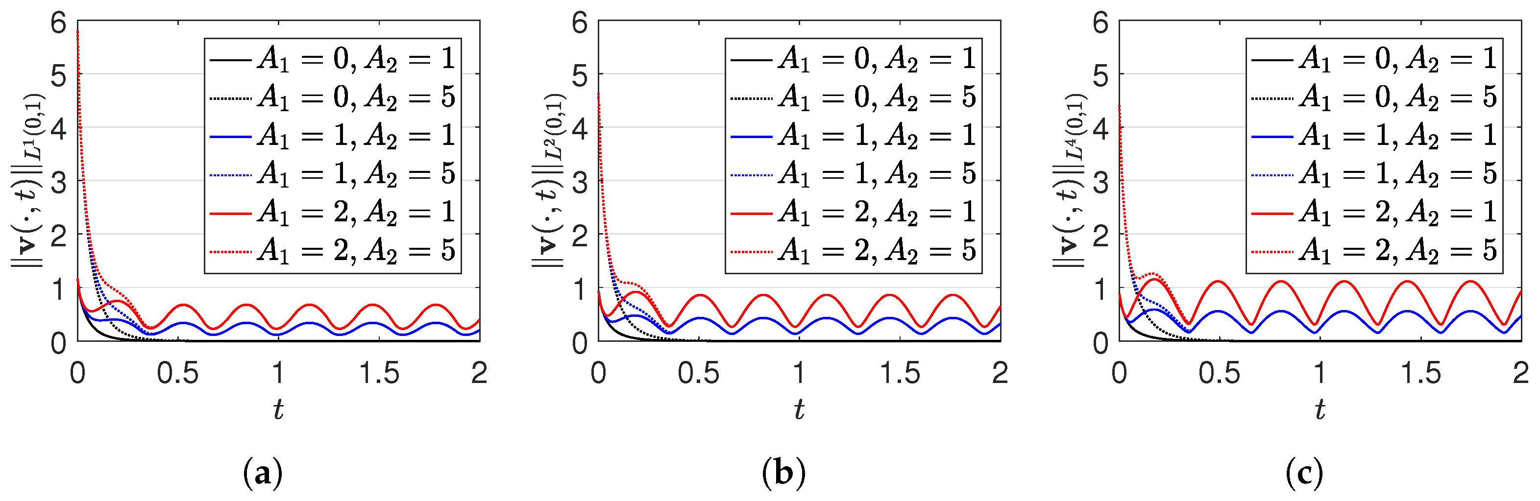
In this section, we present numerical results on the ISS in the $L^q$-norm for system (1) when $q=1$, $q=2$, and $q=4$, respectively.

In simulations, we always set

$$\begin{array}{cc}\hfill n=& 2,a_1=1,a_2=2,b_1=2,b_2=3,\hfill \\ \hfill h_1\left(s\right)=& {\displaystyle \frac{5s}{4\left(5+2s^2\right)}},h_2\left(s\right)={\displaystyle \frac{3tanh\left(s\right)}{10}},\hfill \end{array}$$

for which $b_i>0$, $i=1,2$, and the small-gain condition (7) is satisfied.

In addition, we set

$$\begin{array}{cc}\hfill f_1(x,t)& =f_2(x,t)=d_2\left(t\right)=g_1\left(t\right)=g_2\left(t\right)=0,d_1\left(t\right)=A_{1}sin\left(10t\right),\hfill \\ \hfill v_{01}& =A_{2}sin\left(x\right),v_{02}=A_{2}sin\left(2x\right),\hfill \end{array}$$

where $A_1\in \{0,1,2\}$ and $A_2\in \{1,5\}$ describe the amplitudes of disturbance and initial data, respectively.

Figure 1 presents the evolution of the $L^q$-norm of the solution to system (1) with $q=1,2,4$, respectively, under different initial data and disturbances. The black solid and dashed lines in Figure 1a–c indicate that in the absence of disturbances, the system remains asymptotically stable despite different initial data. The blue solid and red solid lines (or blue dashed and red dashed lines) in Figure 1a–c demonstrate that, for the same initial data, the norm of the solution decreases as the amplitude of the disturbances diminishes. It is noteworthy that due to the exponential decay property of the solution (see (11) and (12)), the norms of the solution under different initial data rapidly converge to zero. Moreover, as time tends to infinity, the ultimate bound of the norms of the solution is primarily determined by the disturbances rather than the initial data. This property is reflected in both the solid and dashed lines, indicating that although the initial data differ, the norms of the solution admit nearly identical bounds for sufficiently large time with the same disturbances. The six lines in either Figure 1a–c effectively illustrate the ISS property of the coupled system.

5. Conclusions

This paper investigates the ISS in different norms for a class of coupled nonlinear parabolic PDEs with in-domain disturbances and Dirichlet boundary disturbances. By employing the generalized Lyapunov method, we first prove the continuous dependence of solutions in the $L^q$-norm for $q\in \left[1,+\infty \right)$, and then establish the ISS estimates for the system through the density argument. The key to this approach lies in the construction of disturbance-dependent positive semi-definite functionals, which overcome the limitations of the classical Lyapunov method in handling Dirichlet boundary disturbances. The work presented in this paper provides new insights for the ISS analysis of coupled nonlinear PDEs with Dirichlet boundary disturbances. It is worth mentioning that, as indicated in Remark 1, the ISS small-gain condition (4) or (7) is related to n, i.e., the number of subsystems. Consequently, deriving the ISS of the coupled system as $n\to \infty$ remains a challenge. In the future, we will devote our efforts to employing the generalized Lyapunov method to establish the ISS for a broader class of PDEs with boundary disturbances. Moreover, since the generalized Lyapunov method may not be universally applicable to any given PDE, developing a unified method within the Lyapunov framework for the ISS analysis of PDEs having a general form will be our ongoing effort.

References

1. Mironchenko, A.; Prieur, C. Input-to-state stability of infinite-dimensional systems: Recent results and open questions. SIAM Rev. 2020, 62, 529–614. [Google Scholar] [CrossRef]
2. Logemann, H. Stabilization of well-posed infinite-dimensional systems by dynamic sampled-data feedback. SIAM J. Control Optim. 2013, 51, 1203–1231. [Google Scholar] [CrossRef][Green Version]
3. Dashkovskiy, S.; Mironchenko, A. Input-to-state stability of infinite-dimensional control systems. Math. Control Signals Syst. 2013, 25, 1–35. [Google Scholar] [CrossRef]
4. Karafyllis, I.; Krstic, M. Input-to-State Stability for PDEs; Springer: Cham, Switzerland, 2019. [Google Scholar]
5. Schwenninger, F.L. Input-to-state stability for parabolic boundary control: Linear and semilinear systems. In Control Theory of Infinite-Dimensional Systems; Kerner, J., Laasri, H., Mugnolo, D., Eds.; Birkhäuser: Cham, Switzerland, 2020; pp. 83–116. [Google Scholar]
6. Zheng, J.; Zhu, G. Input-to-state stability for a class of one-dimensional nonlinear parabolic PDEs with nonlinear boundary conditions. SIAM J. Control Optim. 2020, 58, 2567–2587. [Google Scholar] [CrossRef]
7. Zheng, J.; Zhu, G. Global ISS for the viscous Burgers’ equation with Dirichlet boundary disturbances. IEEE Trans. Autom. Control 2024, 69, 7174–7181. [Google Scholar] [CrossRef]
8. Zheng, J.; Zhu, G. Generalized Lyapunov functionals for the input-to-state stability of infinite-dimensional systems. Automatica 2025, 172, 112005. [Google Scholar] [CrossRef]
9. Bi, Y.; Zheng, J.; Zhu, G. Input-to-state stabilization of 1-D parabolic PDEs under output feedback control. IEEE Trans. Autom. Control 2026, 71, 2692–2699. [Google Scholar] [CrossRef]
10. Deutscher, J. Cooperative output regulation for a network of parabolic systems with varying parameters. Automatica 2021, 125, 109446. [Google Scholar] [CrossRef]
11. Meurer, T.; Krstic, M. Finite-time multi-agent deployment: A nonlinear PDE motion planning approach. Automatica 2011, 47, 2534–2542. [Google Scholar] [CrossRef]
12. Pilloni, A.; Pisano, A.; Orlov, Y.; Usai, E. Consensus-based control for a network of diffusion PDEs with boundary local interaction. IEEE Trans. Autom. Control 2016, 61, 2708–2713. [Google Scholar] [CrossRef]
13. Kabalan, A.; Ferrante, F.; Casadei, G.; Cristofaro, A.; Prieur, C. Leader-follower synchronization of a network of boundary-controlled parabolic equations with in-domain coupling. IEEE Control Syst. Lett. 2021, 6, 2006–2011. [Google Scholar] [CrossRef]
14. Zong, X.; Zheng, J.; Wei, J.; Yang, J. Synchronizing controller design for networked heat equations with boundary structured time-varying perturbations and general disturbances. J. Process Control 2021, 107, 94–102. [Google Scholar] [CrossRef]
15. Yang, Z.; Xu, D. Global dynamics for non-autonomous reaction-diffusion neural networks with time-varying delays. Theor. Comput. Sci. 2008, 403, 3–10. [Google Scholar] [CrossRef]
16. Liang, J.; Cao, J. Global exponential stability of reaction–diffusion recurrent neural networks with time-varying delays. Phys. Lett. A 2003, 314, 434–442. [Google Scholar] [CrossRef]
17. Hu, C.; Jiang, H.; Teng, Z. Impulsive control and synchronization for delayed neural networks with reaction–diffusion terms. IEEE Trans. Neural Netw. 2010, 21, 67–81. [Google Scholar] [PubMed]
18. Shanmugam, L.; Mani, P.; Rajan, R.; Joo, Y.H. Adaptive synchronization of reaction–diffusion neural networks and its application to secure communication. IEEE Trans. Cybern. 2020, 50, 911–922. [Google Scholar] [CrossRef] [PubMed]
19. Mironchenko, A. Input-to-state stability of distributed parameter systems. arXiv 2023, arXiv:2302.00535. [Google Scholar]
20. Zheng, J.; Zhu, G.; Dashkovskiy, S. Relative stability in the sup-norm and input-to-state stability in the sup-norm for parabolic PDEs. IEEE Trans. Autom. Control 2022, 67, 5361–5375. [Google Scholar] [CrossRef]
21. Ladyženskaja, O.A.; Solonnikov, V.A.; Uralćeva, N.N. Linear and Quasi-Linear Equations of Parabolic Type; American Mathematical Society: Providence, RI, USA, 1968. [Google Scholar]
22. Evans, L.C. Partial Differential Equations; American Mathematical Society: Providence, RI, USA, 2010. [Google Scholar]
23. Zheng, J.; Zhu, G. Approximations of Lyapunov functionals for ISS analysis of a class of higher dimensional nonlinear parabolic PDEs. Automatica 2021, 125, 109414. [Google Scholar] [CrossRef]
Figure 1. Evolution of v ( · , t ) L q ( 0 , 1 ) for system (1) with (a) q = 1 , (b) q = 2 , and (c) q = 4 , respectively.
Mathematics 14 02120 g001
Disclaimer/Publisher’s Note: The statements, opinions and data contained in all publications are solely those of the individual author(s) and contributor(s) and not of MDPI and/or the editor(s). MDPI and/or the editor(s) disclaim responsibility for any injury to people or property resulting from any ideas, methods, instructions or products referred to in the content.