Multiplication Semigroups in Variable Exponent Lebesgue Spaces

Abstract

This paper studies multiplication operators and their associated strongly continuous semigroups acting on variable exponent Lebesgue spaces. We study the abstract Cauchy problem $\dot{u}\left(t\right)=Au\left(t\right)$, $u\left(0\right)=u_0$, in the space $L^{p\left(x\right)}(0,\mathsf{\ell })$ with $\mathsf{\ell }>0$, where the generator A is given by the multiplication operator $A=M_q$. Using the modular ${\rho }_{p(·)}\left(u\right)={\int }_0^{\mathsf{\ell }}{\left|u\left(x\right)\right|}^{p\left(x\right)}dx$, we establish the fundamental properties of $M_q$, including ${\rho }_{p(·)}$-closedness, density of its domain, and boundedness criteria in terms of the essential range of q. We show that $M_q$ generates a strongly continuous semigroup ${\left(S\left(t\right)\right)}_{t\ge 0}$ given explicitly by $S\left(t\right)=e^{tA}=M_{e^{tq}}$, and we derive modular growth estimates for the semigroup. We also obtain a complete characterization of the spectrum and resolvent of A, showing that $\sigma \left(A\right)=q_{\mathrm{ess}}(0,\mathsf{\ell })$ and $R(\lambda ,A)={(\lambda I-A)}^{-1}=M_{1/(\lambda -q)}$ for $\lambda \notin \sigma \left(A\right)$. The spectral mapping behavior of the associated semigroup is also analyzed, highlighting the validity of the weak spectral mapping theorem and the possible failure of the full spectral identity. As an application, we present a concrete example on $(0,4)$ involving a singular initial datum that does not belong to $L^2(0,4)$ but lies in $L^{p\left(x\right)}(0,4)$ due to a suitable spatial variation of the exponent. The corresponding evolution is explicitly given by $u(t,x)=e^{tq\left(x\right)}f\left(x\right)$ and remains well posed in $L^{p\left(x\right)}(0,4)$ for all $t\ge 0$. This shows that the variable exponent framework can accommodate singular behavior while preserving semigroup dynamics. These results show that multiplication operators provide an explicit model for semigroup theory in variable exponent spaces, connecting modular analysis with pointwise evolution equations.

1. Introduction

Strongly continuous semigroups constitute one of the fundamental tools in the study of time-dependent phenomena arising in differential equations, mathematical physics, control theory, and applied analysis. They provide an operator theory approach that allows many evolution problems to be treated through the properties of their infinitesimal generators. In the classical setting of Banach spaces, semigroup methods have been extensively used to establish existence, uniqueness, regularity, and stability results for abstract evolution equations of the form

$${\displaystyle \frac{d}{dt}}u\left(t\right)=Bu\left(t\right),t\ge 0,u\left(0\right)=u_0,$$

(1)

where B is a generally unbounded linear operator acting on a Banach space; see, for example, [1,2,3,4].

While this theory is well developed in classical spaces such as $L^p(0,\mathsf{\ell })$ with constant exponent, it becomes insufficient in situations where the underlying phenomena exhibit spatial heterogeneity, nonstandard growth conditions, or localized singular behavior. In such cases, the assumption of uniform integrability across the domain may be too restrictive and may fail to capture important local features of the solution.

To overcome these limitations, variable exponent Lebesgue spaces $L^{p\left(x\right)}(0,\mathsf{\ell })$ have emerged as a natural generalization of the classical $L^p$-spaces. By allowing the exponent p to depend on the spatial variable, these spaces provide a flexible setting capable of adapting to local regularity and integrability properties. In particular, they enable the treatment of problems with spatially varying growth and local singular behavior. Such spaces have found important applications in nonlinear partial differential equations, electrorheological fluids, image restoration, and related problems with nonstandard growth conditions; see, for example, [5,6,7,8,9].

The analysis in $L^{p\left(x\right)}$-spaces is naturally formulated in terms of the modular

$${\rho }_{p(·)}\left(u\right)={\int }_0^{\mathsf{\ell }}{\left|u\left(x\right)\right|}^{p\left(x\right)}dx,$$

where convergence and continuity are described through the modular rather than solely through the norm. This approach has been extensively developed in the theory of modular spaces and generalized function spaces; see, for example, [6,10,11]. More recently, semigroup methods in modular function spaces have been investigated in [12,13], where modular analogues of strongly continuous semigroups and evolution Equations were introduced.

The purpose of this paper is to study multiplication operators and the strongly continuous semigroups they generate in the variable exponent space $L^{p\left(x\right)}(0,\mathsf{\ell })$. Particular attention is devoted to the modular properties of these operators, including ${\rho }_{p(·)}$ closedness, density of the domain, boundedness, invertibility, and spectral characterization. We also investigate the associated multiplication semigroups, establish modular growth estimates, and analyze their spectral behavior. The analysis is carried out directly with respect to the modular ${\rho }_{p(·)}$ and does not rely on the classical norm-based semigroup theory. For the classical theory of strongly continuous semigroups and evolution equations, we refer to [1,2].

Before studying nonlinear variable exponent evolution equations, it is useful to understand the behavior of semigroups in $L^{p\left(x\right)}(0,\mathsf{\ell })$ itself. As emphasized in [6] (pp. 9–10), several properties that play a central role in the classical $L^p$-theory do not generally remain valid in variable exponent spaces. Examples include the boundedness of translation operators, standard convolution estimates, and other tools that are routinely used in the analysis of evolution equations. Consequently, semigroup properties in $L^{p\left(x\right)}(0,\mathsf{\ell })$ often need to be established directly through the modular structure rather than obtained as straightforward extensions of the classical theory.

A key ingredient in the analysis is the use of Steklov-type averaging and modular convergence techniques, which allow us to justify differentiation in the modular sense and to establish the connection between a semigroup and its infinitesimal generator. These methods are closely related to modular approximation techniques that appear in generalized function spaces and nonlinear approximation theory; see, for example, [14,15].

To illustrate the abstract results, we investigate multiplication semigroups on $L^{p\left(x\right)}(0,\mathsf{\ell })$, where the associated evolution problem reduces to a family of pointwise ordinary differential equations. This class of examples provides an explicit connection between semigroup dynamics and the local structure induced by the exponent function $p\left(x\right)$.

As an application, we study semigroup well-posedness for evolution problems involving singular initial data. We construct examples in which the initial datum fails to belong to the classical space $L^2(0,\mathsf{\ell })$ because of localized singularities, while remaining admissible in a suitable variable exponent space $L^{p\left(x\right)}(0,\mathsf{\ell })$. This illustrates the flexibility of the variable exponent setting in handling localized irregular behavior that cannot generally be treated within the classical fixed exponent setting.

The rest of the paper is organized as follows. Section 2 recalls the variable exponent Lebesgue space $L^{p\left(x\right)}(0,\mathsf{\ell })$, its modular structure, and the associated Luxemburg norm. Section 3 develops the abstract evolution framework in $L^{p\left(x\right)}(0,\mathsf{\ell })$; we introduce modularly strongly continuous semigroups and their infinitesimal generators, formulate the associated abstract Cauchy problem, and establish semigroup generation and modular growth estimates. Section 4 applies the abstract theory to multiplication operators, characterizes the corresponding multiplication semigroups and their spectral properties, and presents examples involving singular initial data in variable exponent spaces. Finally, Section 5 discusses perspectives and possible extensions of the proposed theory.

2. Variable Exponent Lebesgue Spaces ${\mathit{L}}^{\mathit{p}\mathbf{\left(}\mathit{x}\mathbf{\right)}}\mathbf{(}\mathbf{0}\mathbf{,}\mathsf{\ell }\mathbf{)}$

In this section, we recall the basic definitions and properties of the variable exponent space $L^{p\left(x\right)}(0,\mathsf{\ell })$ and its associated modular. These notions provide the functional analysis foundation for the semigroup theory developed in the subsequent sections.

Denote by $L^0(0,\mathsf{\ell })$ the space of all real-valued Lebesgue measurable functions on $(0,\mathsf{\ell })$. The variable exponent Lebesgue space $L^{p\left(x\right)}(0,\mathsf{\ell })$ is defined by

$$L^{p\left(x\right)}(0,\mathsf{\ell })=\left\{u\in L^0(0,\mathsf{\ell }):{\rho }_{p(·)}\left(\lambda u\right)<\infty \mathrm{for}\mathrm{some}\lambda >0\right\},$$

(2)

where the modular functional is given by

$${\rho }_{p(·)}\left(u\right)={\int }_0^{\mathsf{\ell }}{\left|u\left(x\right)\right|}^{p\left(x\right)}dx.$$

(3)

The associated Luxemburg norm is defined by

$${\parallel u\parallel }_{p(·)}=\inf \left\{\lambda >0:{\rho }_{p(·)}\left({\displaystyle \frac{u}{\lambda }}\right)\le 1\right\}.$$

(4)

Throughout this paper, we assume that

$$1<p_{-}\le p\left(x\right)\le p_{+}<\infty ,x\in (0,\mathsf{\ell }).$$

(5)

Under this assumption, $L^{p\left(x\right)}(0,\mathsf{\ell })$ is a separable and reflexive Banach space; see [5,6,16].

The modular ${\rho }_{p(·)}$ is convex and satisfies

$${\rho }_{p(·)}(\alpha u+(1-\alpha )v)\le \alpha {\rho }_{p(·)}\left(u\right)+(1-\alpha ){\rho }_{p(·)}\left(v\right),\alpha \in [0,1],u,v\in L^{p\left(x\right)}(0,\mathsf{\ell }).$$

(6)

Moreover,

$${\rho }_{p(·)}\left(u\right)=0⟺u=0,$$

and

$${\rho }_{p(·)}\left(\alpha u\right)={\rho }_{p(·)}\left(u\right)\mathrm{whenever}\left|\alpha \right|=1.$$

Hence, ${\rho }_{p(·)}$ is a convex regular modular in the sense of Khamsi and Kozłowski [11].

Since $p\left(x\right)\le p_{+}$ almost everywhere on $(0,\mathsf{\ell })$, the modular satisfies the ${\Delta }_2$ condition

$${\rho }_{p(·)}\left(2u\right)={\int }_0^{\mathsf{\ell }}{2}^{p\left(x\right)}{\left|u\left(x\right)\right|}^{p\left(x\right)}dx\le 2^{p_{+}}{\rho }_{p(·)}\left(u\right),u\in L^{p\left(x\right)}(0,\mathsf{\ell }).$$

(7)

Consequently, modular convergence and norm convergence are equivalent; see [6,11].

Associated with the modular ${\rho }_{p(·)}$, we define the growth function by

$${\omega }_{p(·)}\left(t\right):=\sup \left\{{\displaystyle \frac{{\rho }_{p(·)}\left(tu\right)}{{\rho }_{p(·)}\left(u\right)}}:0<{\rho }_{p(·)}\left(u\right)<\infty \right\},t>0.$$

(8)

For the space $L^{p\left(x\right)}(0,\mathsf{\ell })$,

$${\rho }_{p(·)}\left(tu\right)={\int }_0^{\mathsf{\ell }}{t}^{p\left(x\right)}{\left|u\left(x\right)\right|}^{p\left(x\right)}dx,u\in L^{p\left(x\right)}(0,\mathsf{\ell }),$$

and therefore

$${\omega }_{p(·)}\left(t\right)=\underset{x\in (0,\mathsf{\ell })}{\mathrm{ess}\hspace{0.17em}\sup \hspace{0.17em}}{t}^{p\left(x\right)}.$$

Since the function $a\mapsto t^a$ is decreasing for $0<t<1$ and increasing for $t>1$, it follows that

$${\omega }_{p(·)}\left(t\right)=\left\{\begin{array}{cc}{t}^{p_{-}},\hfill & 0<t<1,\hfill \\ 1,\hfill & t=1,\hfill \\ t^{p_{+}},\hfill & t>1.\hfill \end{array}\right.$$

(9)

In particular,

$${\omega }_{p(·)}\left(2\right)=2^{p_{+}}=K_{{\Delta }_2}.$$

Using the inequality

$${|a+b|}^{\theta }\le 2^{\theta -1}\left({\left|a\right|}^{\theta }+{\left|b\right|}^{\theta }\right),\theta \ge 1,$$

we obtain for almost every $x\in (0,\mathsf{\ell })$,

$${|u\left(x\right)+v\left(x\right)|}^{p\left(x\right)}\le 2^{p_{+}-1}\left({\left|u\left(x\right)\right|}^{p\left(x\right)}+{\left|v\left(x\right)\right|}^{p\left(x\right)}\right).$$

Integrating over $(0,\mathsf{\ell })$ yields, for $u,v\in L^{p\left(x\right)}(0,\mathsf{\ell })$,

$${\rho }_{p(·)}(u+v)\le 2^{p_{+}-1}\left({\rho }_{p(·)}\left(u\right)+{\rho }_{p(·)}\left(v\right)\right)={\displaystyle \frac{{\omega }_{p(·)}\left(2\right)}{2}}\left({\rho }_{p(·)}\left(u\right)+{\rho }_{p(·)}\left(v\right)\right).$$

(10)

Thus, in the variable exponent case, the constants appearing in (9) and (10) are determined by the essential bounds $p_{-}$ and $p_{+}$ of the exponent function. These estimates will be used repeatedly in the analysis of operators and semigroups on $L^{p\left(x\right)}(0,\mathsf{\ell })$. We now introduce the notions of ${\rho }_{p(·)}$-bounded operators and strongly continuous semigroups on $L^{p\left(x\right)}(0,\mathsf{\ell })$. The definitions adopted below are based on the modular theory of Khamsi and Kozłowski [11]; see also Bachar [13].

Definition 1

(${\rho }_{p(·)}$–bounded operator [13]). A linear operator $B:L^{p\left(x\right)}(0,\mathsf{\ell })\to L^{p\left(x\right)}(0,\mathsf{\ell })$ is called ${\rho }_{p(·)}$-bounded if there exists a constant $M_B\ge 0$ such that

$${\rho }_{p(·)}\left(Bf\right)\le M_B{\rho }_{p(·)}\left(f\right),f\in L^{p\left(x\right)}(0,\mathsf{\ell }).$$

The infimum of all such constants $M_B$ is called the ${\rho }_{p(·)}$-bound of B.

The following result gives the relation between ${\rho }_{p(·)}$-boundedness and boundedness with respect to the Luxemburg norm under assumption (5). It is obtained by adapting the corresponding modular-space argument from Bachar [13] to the variable exponent space $L^{p\left(x\right)}(0,\mathsf{\ell })$.

Lemma 1

([11,13]). Assume that (5) holds. Let $B\in \mathcal{L}\left(L^{p\left(x\right)}(0,\mathsf{\ell })\right)$ be ${\rho }_{p(·)}$-bounded with constant $M_B$ as in Definition 1. Then,

$${\parallel Bf\parallel }_{p(·)}\le C_B{\parallel f\parallel }_{p(·)},f\in L^{p\left(x\right)}(0,\mathsf{\ell }),$$

where

$$C_B=\max \left\{M_B^{1/p^{-}},M_B^{1/p^{+}}\right\}.$$

Proof. 

If $M_B=0$, then

$${\rho }_{p(·)}\left(Bf\right)=0,f\in L^{p\left(x\right)}(0,\mathsf{\ell }),$$

and therefore $Bf=0$ for every $f\in L^{p\left(x\right)}(0,\mathsf{\ell })$. The conclusion is then immediate. Hence, assume that $M_B>0$.

Let $f\in L^{p\left(x\right)}(0,\mathsf{\ell })$ satisfy

$${\parallel f\parallel }_{p(·)}\le 1.$$

By the norm-modular relation (see [6] (Lemma 3.2.4)),

$${\rho }_{p(·)}\left(f\right)\le 1.$$

Since B is ${\rho }_{p(·)}$-bounded,

$${\rho }_{p(·)}\left(Bf\right)\le M_B{\rho }_{p(·)}\left(f\right)\le M_B.$$

Assume first that $M_B\ge 1$. Then,

$${\rho }_{p(·)}\left({\displaystyle \frac{Bf}{M_B^{1/p^{-}}}}\right)={\int }_0^{\mathsf{\ell }}{M}_B^{-p\left(x\right)/p^{-}}{\left|Bf\left(x\right)\right|}^{p\left(x\right)}dx.$$

Since $p\left(x\right)\ge p^{-}$ and $M_B\ge 1$,

$$M_B^{-p\left(x\right)/p^{-}}\le M_B^{-1}.$$

Therefore,

$${\rho }_{p(·)}\left({\displaystyle \frac{Bf}{M_B^{1/p^{-}}}}\right)\le {\displaystyle \frac{1}{M_B}}{\rho }_{p(·)}\left(Bf\right)\le 1.$$

By the definition of the Luxemburg norm,

$${\parallel Bf\parallel }_{p(·)}\le M_B^{1/p^{-}}.$$

Next, assume that $0<M_B\le 1$. Then,

$${\rho }_{p(·)}\left({\displaystyle \frac{Bf}{M_B^{1/p^{+}}}}\right)={\int }_0^{\mathsf{\ell }}{M}_B^{-p\left(x\right)/p^{+}}{\left|Bf\left(x\right)\right|}^{p\left(x\right)}dx.$$

Since $p\left(x\right)\le p^{+}$ and $0<M_B\le 1$,

$$M_B^{-p\left(x\right)/p^{+}}\le M_B^{-1}.$$

Hence,

$${\rho }_{p(·)}\left({\displaystyle \frac{Bf}{M_B^{1/p^{+}}}}\right)\le {\displaystyle \frac{1}{M_B}}{\rho }_{p(·)}\left(Bf\right)\le 1,$$

which implies that

$${\parallel Bf\parallel }_{p(·)}\le M_B^{1/p^{+}}.$$

Combining the two cases, we obtain

$${\parallel Bf\parallel }_{p(·)}\le \max \left\{M_B^{1/p^{-}},M_B^{1/p^{+}}\right\}$$

whenever ${\parallel f\parallel }_{p(·)}\le 1$.

Let $f\in L^{p\left(x\right)}(0,\mathsf{\ell })$ be such that $f\ne 0$, and set

$$g:={\displaystyle \frac{f}{{\parallel f\parallel }_{p(·)}}}.$$

Then ${\parallel g\parallel }_{p(·)}=1$. Applying the previous estimate to g, we obtain

$${\parallel Bg\parallel }_{p(·)}\le \max \left\{M_B^{1/p^{-}},M_B^{1/p^{+}}\right\}.$$

Using the linearity of B and the homogeneity of the Luxemburg norm, it follows that

$${\parallel Bf\parallel }_{p(·)}={\parallel f\parallel }_{p(·)}{\parallel Bg\parallel }_{p(·)}\le \max \left\{M_B^{1/p^{-}},M_B^{1/p^{+}}\right\}{\parallel f\parallel }_{p(·)}.$$

Since the estimate is trivial for $f=0$, it holds for all $f\in L^{p\left(x\right)}(0,\mathsf{\ell })$. □

Definition 2

(Strongly continuous semigroup [11,13]). A family ${\left(S\left(t\right)\right)}_{t\ge 0}$ of operators on $L^{p\left(x\right)}(0,\mathsf{\ell })$ is called a strongly continuous semigroup if the following conditions hold:

(i) 

$S\left(0\right)=I_{L^{p\left(x\right)}(0,\mathsf{\ell })},$ where $I_{L^{p\left(x\right)}(0,\mathsf{\ell })}$ denotes the identity operator on $L^{p\left(x\right)}(0,\mathsf{\ell })$;

(ii) 

$S(t+s)=S\left(t\right)S\left(s\right),t,s\ge 0;$

(iii) 

for every $f\in L^{p\left(x\right)}(0,\mathsf{\ell })$, the orbit $t\mapsto S\left(t\right)f$ is continuous with respect to the modular ${\rho }_{p(·)}$, that is, for every $t_0\ge 0$,

$${\rho }_{p(·)}\left(S\left(t\right)f-S\left(t_0\right)f\right)\to 0\mathrm{as}t\to t_0.$$

If only conditions (i)–(ii) are satisfied, the family ${\left(S\left(t\right)\right)}_{t\ge 0}$ is called a semigroup on $L^{p\left(x\right)}(0,\mathsf{\ell })$.

If, in addition, each operator $S\left(t\right)$ is ${\rho }_{p(·)}$-bounded, then continuity at an arbitrary time $t_0\ge 0$ follows from continuity at $t=0$. Indeed, for $t\ge t_0$, the semigroup property yields

$$S\left(t\right)f-S\left(t_0\right)f=S\left(t_0\right)\left(S(t-t_0)f-f\right),$$

and therefore

$${\rho }_{p(·)}\left(S\left(t\right)f-S\left(t_0\right)f\right)\le M_{t_0}{\rho }_{p(·)}\left(S(t-t_0)f-f\right),$$

where $M_{t_0}$ denotes the ${\rho }_{p(·)}$-bound of $S\left(t_0\right)$.

Consequently, if

$${\rho }_{p(·)}\left(S\left(h\right)f-f\right)\to 0\mathrm{as}h\to 0^{+},$$

then,

$${\rho }_{p(·)}\left(S\left(t\right)f-S\left(t_0\right)f\right)\to 0\mathrm{as}t\to t_0^{+}.$$

Hence, for ${\rho }_{p(·)}$-bounded semigroups, strong continuity is completely determined by continuity at $t=0$.

In this case, the infinitesimal generator B associated with ${\left(S\left(t\right)\right)}_{t\ge 0}$ is defined by

$$Bf=g,$$

whenever there exists $g\in L^{p\left(x\right)}(0,\mathsf{\ell })$ such that

$$\underset{t\downarrow 0}{\lim }{\rho }_{p(·)}\left({\displaystyle \frac{S\left(t\right)f-f}{t}}-g\right)=0.$$

The domain of B is defined by

$$D\left(B\right):=\left\{f\in L^{p\left(x\right)}(0,\mathsf{\ell }):\exists g\in L^{p\left(x\right)}(0,\mathsf{\ell })\mathrm{such}\mathrm{that}\underset{t\downarrow 0}{\lim }{\rho }_{p(·)}\left({\displaystyle \frac{S\left(t\right)f-f}{t}}-g\right)=0\right\}.$$

The concepts introduced above provide the basic semigroup tools required for the study of abstract evolution equations in $L^{p\left(x\right)}(0,\mathsf{\ell })$. In the next section, we investigate the associated Cauchy problem and establish existence, uniqueness, and continuous dependence of solutions in $L^{p\left(x\right)}(0,\mathsf{\ell })$.

3. Abstract Evolution Problem and Semigroup Approach

Strongly continuous semigroups provide a powerful tool for the analysis of abstract differential equations and their applications to ordinary, functional, and partial differential equations; see, for example, [1,2,3]. In the classical theory, evolution equations are typically studied in Banach spaces such as $L^p$-spaces. In the present work, we consider such problems in the variable exponent space $L^{p\left(x\right)}(0,\mathsf{\ell })$, whose modular structure was described in the previous section.

We study the abstract Cauchy problem

$$\begin{array}{cc}\hfill {\displaystyle \frac{d}{dt}}u\left(t\right)& =Bu\left(t\right),t\ge 0,\hfill \end{array}$$

(11a)

$$\begin{array}{cc}\hfill u\left(0\right)& =u_0,\hspace{1em}\hspace{1em}\hspace{1em}\hspace{1em}\hfill \end{array}$$

(11b)

where

$$B:D\left(B\right)\subset L^{p\left(x\right)}(0,\mathsf{\ell })\to L^{p\left(x\right)}(0,\mathsf{\ell })$$

is the infinitesimal generator of a strongly continuous semigroup ${\left(S\left(t\right)\right)}_{t\ge 0}$.

Equation (11) serves as the basic model for linear evolution processes in $L^{p\left(x\right)}(0,\mathsf{\ell })$. Whenever $u_0\in D\left(B\right)$, the corresponding solution is formally given by

$$u\left(t\right)=S\left(t\right)u_0,t\ge 0.$$

Our aim is to investigate the existence, uniqueness, continuity, and growth properties of solutions of (11) and to establish the connection between the semigroup ${\left(S\left(t\right)\right)}_{t\ge 0}$ and its infinitesimal generator B. The approach adopted here is inspired by the classical semigroup theory of Pazy [1], Engel and Nagel [2], and Ito and Kappel [3], while being formulated in terms of the modular ${\rho }_{p(·)}$.

The following notion of solution is adapted from the classical semigroup theory of Engel and Nagel [2], Pazy [1], and the modular approach developed in [13].

Definition 3

([13]). Let $u_0\in L^{p\left(x\right)}(0,\mathsf{\ell })$. A function $u:[0,\infty )\to L^{p\left(x\right)}(0,\mathsf{\ell })$ is said to solve (11) if the following requirements are fulfilled:

(i) 

There exists an element $v\in L^{p\left(x\right)}(0,\mathsf{\ell })$ such that

$$\underset{h\to 0^{+}}{\lim }{\rho }_{p(·)}\left({\displaystyle \frac{u\left(h\right)-u\left(0\right)}{h}}-v\right)=0.$$

In this case, we denote v by ${\dot{u}}_{+}\left(0\right)$.

(ii) 

For every $t>0$, there exists $\dot{u}\left(t\right)\in L^{p\left(x\right)}(0,\mathsf{\ell })$ satisfying

$$\underset{h\to 0}{\lim }{\rho }_{p(·)}\left({\displaystyle \frac{u(t+h)-u\left(t\right)}{h}}-\dot{u}\left(t\right)\right)=0.$$

(iii) 

The mapping $t\mapsto \dot{u}\left(t\right)$ is continuous on $(0,\infty )$ with respect to the modular topology induced by ${\rho }_{p(·)}$.

(iv) 

The trajectory remains in the domain of the generator, that is,

$$u\left(t\right)\in D\left(B\right),t\ge 0.$$

(v) 

The evolution law is satisfied in $L^{p\left(x\right)}(0,\mathsf{\ell })$: $\dot{u}\left(t\right)=Bu\left(t\right),t>0,$ together with the initial condition $u\left(0\right)=u_0$.

The following result shows that every ${\rho }_{p(·)}$-bounded operator generates a strongly continuous semigroup on $L^{p\left(x\right)}(0,\mathsf{\ell })$. The construction is based on the exponential series and may be viewed as the modular analogue of the classical bounded generator theorem in Banach spaces; see [1,2]. For the corresponding result in modular spaces, we refer to [13].

Lemma 2

([13]). Let $p:(0,\mathsf{\ell })\to (1,\infty )$ satisfy (5), and let ${\rho }_{p(·)}$ be the associated modular on $L^{p\left(x\right)}(0,\mathsf{\ell })$. Let $B\in \mathcal{L}\left(L^{p\left(x\right)}(0,\mathsf{\ell })\right)$ be ${\rho }_{p(·)}$–bounded with constant $M_B>0$. For $t\ge 0$, define

$$S\left(t\right)\varphi :={\displaystyle \sum _{n=0}^{\infty }}{\displaystyle \frac{t^n}{n!}}{B}^n\varphi ,\varphi \in L^{p\left(x\right)}(0,\mathsf{\ell }),$$

where the series converges in the modular sense. Then, ${\left\{S\left(t\right)\right\}}_{t\ge 0}$ forms a strongly continuous semigroup on $L^{p\left(x\right)}(0,\mathsf{\ell })$, satisfying $S\left(0\right)=I$ and $S(t+s)=S\left(t\right)S\left(s\right)$ for all $t,s\ge 0$. Moreover, for all $t\ge 0$ and $\varphi \in L^{p\left(x\right)}(0,\mathsf{\ell })$, we have

$${\rho }_{p(·)}\left(S\left(t\right)\varphi \right)\le e^{(p_{+}-1)t}{e}^{M_{B}t}{\rho }_{p(·)}\left(\varphi \right)=e^{(M_B+p_{+}-1)t}{\rho }_{p(·)}\left(\varphi \right).$$

(12)

Proof. 

The proof follows the modular semigroup construction developed in [13]. Under assumption (5), the modular ${\rho }_{p(·)}$ defined in (3) is convex, and its associated growth function ${\omega }_{p(·)}$ is given by (9). In particular, since $e^t\ge 1$ for all $t\ge 0$, one has

$${\omega }_{p(·)}\left(e^t\right)=e^{t{p}_{+}},{\displaystyle \frac{{\omega }_{p(·)}\left(e^t\right)}{e^t}}=e^{(p_{+}-1)t}.$$

Applying the general modular estimate for exponential series established in [13], together with the ${\rho }_{p(·)}$-boundedness of B, yields

$${\rho }_{p(·)}\left(S\left(t\right)\varphi \right)\le {\displaystyle \frac{{\omega }_{p(·)}\left(e^t\right)}{e^t}}{e}^{M_{B}t}{\rho }_{p(·)}\left(\varphi \right)=e^{(p_{+}-1)t}{e}^{M_{B}t}{\rho }_{p(·)}\left(\varphi \right),$$

which gives (12).

The semigroup property, strong ${\rho }_{p(·)}$-continuity, and the identification of the infinitesimal generator follow directly from the general theory in [13]. □

We now state the Laplace resolvent estimate in the variable exponent space $L^{p\left(x\right)}(0,\mathsf{\ell })$.

Theorem 1

(Laplace resolvent in $L^{p\left(x\right)}(0,\mathsf{\ell })$). Let $p:(0,\mathsf{\ell })\to (1,\infty )$ satisfy (5), and let $B\in \mathcal{L}\left(L^{p\left(x\right)}(0,\mathsf{\ell })\right)$ be ${\rho }_{p(·)}$-bounded with constant $M_B>0$. Let ${\left(S\left(t\right)\right)}_{t\ge 0}$ be the strongly continuous semigroup generated by B as in Lemma 2. Then, for every

$$\lambda >M_B+p_{+}-1,$$

the Laplace integral

$$R(\lambda ,B)\varphi :={\int }_0^{\infty }{e}^{-\lambda t}S\left(t\right)\varphi dt,\varphi \in L^{p\left(x\right)}(0,\mathsf{\ell }),$$

is well defined in $L^{p\left(x\right)}(0,\mathsf{\ell })$ in the modular sense and satisfies

$${\rho }_{p(·)}\left(R(\lambda ,B)\varphi \right)\le {\displaystyle \frac{c_{p(·)}\left(\lambda \right)}{\lambda -(M_B+p_{+}-1)}}{\rho }_{p(·)}\left(\varphi \right),\varphi \in L^{p\left(x\right)}(0,\mathsf{\ell }),$$

where

$$c_{p(·)}\left(\lambda \right)=\left\{\begin{array}{cc}1,\hfill & \lambda \ge 1,\hfill \\ {\lambda }^{1-p_{+}},\hfill & 0<\lambda <1.\hfill \end{array}\right.$$

In particular, $R(\lambda ,B)$ is a ${\rho }_{p(·)}$-bounded linear operator on $L^{p\left(x\right)}(0,\mathsf{\ell })$.

Proof. 

Fix $\lambda >M_B+p_{+}-1$ and $\varphi \in L^{p\left(x\right)}(0,\mathsf{\ell })$. For almost every $x\in (0,\mathsf{\ell })$,

$$R(\lambda ,B)\varphi \left(x\right)={\int }_0^{\infty }{e}^{-\lambda t}S\left(t\right)\varphi \left(x\right)dt={\displaystyle \frac{1}{\lambda }}{\int }_0^{\infty }\lambda e^{-\lambda t}S\left(t\right)\varphi \left(x\right)dt.$$

Since $p\left(x\right)\ge p_{-}>1$ a.e. on $(0,\mathsf{\ell })$, the function

$$s\mapsto {\left|s\right|}^{p\left(x\right)}$$

is convex for almost every $x\in (0,\mathsf{\ell })$. Define the measure

$$d{\mu }_{\lambda }\left(t\right):=\lambda e^{-\lambda t}dt,t\in (0,\infty ).$$

Then, ${\mu }_{\lambda }$ satisfies ${\mu }_{\lambda }\left((0,\infty )\right)=1$, since

$${\int }_0^{\infty }\lambda e^{-\lambda t}dt=1.$$

Hence, for each fixed $x\in (0,\mathsf{\ell })$, we may apply Jensen’s inequality (Theorem 1.4.14 in [6]) to the function $t\mapsto S\left(t\right)\varphi \left(x\right)$, and obtain

$${\left|{\int }_0^{\infty }\lambda e^{-\lambda t}S\left(t\right)\varphi \left(x\right)dt\right|}^{p\left(x\right)}\le {\int }_0^{\infty }\lambda e^{-\lambda t}{\left|S\left(t\right)\varphi \left(x\right)\right|}^{p\left(x\right)}dt.$$

Consequently,

$${\left|R(\lambda ,B)\varphi \left(x\right)\right|}^{p\left(x\right)}={\left|{\displaystyle \frac{1}{\lambda }}{\int }_0^{\infty }\lambda e^{-\lambda t}S\left(t\right)\varphi \left(x\right)dt\right|}^{p\left(x\right)}\le {\lambda }^{-p\left(x\right)}{\int }_0^{\infty }\lambda e^{-\lambda t}{\left|S\left(t\right)\varphi \left(x\right)\right|}^{p\left(x\right)}dt,$$

that is,

$${\left|R(\lambda ,B)\varphi \left(x\right)\right|}^{p\left(x\right)}\le {\lambda }^{1-p\left(x\right)}{\int }_0^{\infty }{e}^{-\lambda t}{\left|S\left(t\right)\varphi \left(x\right)\right|}^{p\left(x\right)}dt.$$

(13)

Using (5), we estimate the factor ${\lambda }^{1-p\left(x\right)}$ by distinguishing two cases.

If $\lambda \ge 1$, then, since $1-p\left(x\right)\le 0$, it follows that

$${\lambda }^{1-p\left(x\right)}\le 1.$$

If $0<\lambda <1$, then the function $a\mapsto {\lambda }^{1-a}$ is increasing on $\mathbb{R}$. Hence, using the bound $p\left(x\right)\le p_{+}$, we obtain

$${\lambda }^{1-p\left(x\right)}\le {\lambda }^{1-p_{+}}.$$

Combining the above estimates, we conclude that, for all $\lambda >0$ and almost every $x\in \Omega$,

$${\lambda }^{1-p\left(x\right)}\le c_{p(·)}\left(\lambda \right),$$

where

$$c_{p(·)}\left(\lambda \right):=\left\{\begin{array}{cc}1,\hfill & \lambda \ge 1,\hfill \\ {\lambda }^{1-p_{+}},\hfill & 0<\lambda <1.\hfill \end{array}\right.$$

Integrating (13) over $(0,\mathsf{\ell })$ with respect to x and applying the Fubini–Tonelli theorem on the product domain $(0,\mathsf{\ell })\times (0,\infty )$, we obtain

$$\begin{array}{cc}\hfill {\rho }_{p(·)}\left(R(\lambda ,B)\varphi \right)& ={\int }_0^{\mathsf{\ell }}{\left|R(\lambda ,B)\varphi \left(x\right)\right|}^{p\left(x\right)}dx\hfill \\ & \le c_{p(·)}\left(\lambda \right){\int }_0^{\infty }{e}^{-\lambda t}\left({\int }_0^{\mathsf{\ell }}{\left|S\left(t\right)\varphi \left(x\right)\right|}^{p\left(x\right)}dx\right)dt\hfill \\ & =c_{p(·)}\left(\lambda \right){\int }_0^{\infty }{e}^{-\lambda t}{\rho }_{p(·)}\left(S\left(t\right)\varphi \right)dt.\hfill \end{array}$$

By Lemma 2,

$${\rho }_{p(·)}\left(S\left(t\right)\varphi \right)\le e^{(M_B+p_{+}-1)t}{\rho }_{p(·)}\left(\varphi \right),t\ge 0.$$

Therefore,

$$\begin{array}{cc}\hfill {\rho }_{p(·)}\left(R(\lambda ,B)\varphi \right)& \le c_{p(·)}\left(\lambda \right){\rho }_{p(·)}\left(\varphi \right){\int }_0^{\infty }{e}^{-(\lambda -(M_B+p_{+}-1))t}dt\hfill \\ & ={\displaystyle \frac{c_{p(·)}\left(\lambda \right)}{\lambda -(M_B+p_{+}-1)}}{\rho }_{p(·)}\left(\varphi \right),\hfill \end{array}$$

since $\lambda >M_B+p_{+}-1$. This proves the claim. □

The resolvent estimate in Theorem 1 is based on the general growth bound (12), which yields the denominator $\lambda -(M_B+p_{+}-1)$. The bound with denominator $\lambda -M_B$ is optimal in this setting, but it requires the stronger semigroup estimate

$${\rho }_{p(·)}\left(S\left(t\right)\varphi \right)\le e^{M_{B}t}{\rho }_{p(·)}\left(\varphi \right),t\ge 0.$$

In the absence of this sharper growth condition, one only obtains the weaker denominator $\lambda -(M_B+p_{+}-1)$, where the additional term $p_{+}-1$ reflects the contribution of the variable exponent modular structure. This distinction can be illustrated by simple multiplication semigroups.

If $B=I$, then $M_B=1$ and

$$S\left(t\right)\varphi =e^t\varphi .$$

Hence

$${\rho }_{p(·)}\left(S\left(t\right)\varphi \right)={\int }_0^{\mathsf{\ell }}|e^t{\varphi \left(x\right)|}^{p\left(x\right)}dx={\int }_0^{\mathsf{\ell }}{e}^{tp\left(x\right)}{\left|\varphi \left(x\right)\right|}^{p\left(x\right)}dx\le e^{p_{+}t}{\rho }_{p(·)}\left(\varphi \right).$$

Since, in this case

$$p_{+}t=(M_B+p_{+}-1)t,$$

this agrees exactly with the general growth bound (12). Thus, the denominator

$$\lambda -(M_B+p_{+}-1)$$

is the natural one in general.

By contrast, if $B=0$, then $M_B=0$ and

$$S\left(t\right)\varphi =\varphi ,$$

so that

$${\rho }_{p(·)}\left(S\left(t\right)\varphi \right)={\rho }_{p(·)}\left(\varphi \right),t\ge 0.$$

Thus, the sharper estimate

$${\rho }_{p(·)}\left(S\left(t\right)\varphi \right)\le e^{M_{B}t}{\rho }_{p(·)}\left(\varphi \right)$$

holds exactly, and the resolvent bound involves the denominator

$$\lambda -M_B=\lambda .$$

This shows that the additional term $p_{+}-1$ is intrinsic to the variable exponent modular structure and reflects the additional growth induced by the variability of the exponent.

The following result provides a modular analogue of the classical regularization of semigroup orbits via Steklov averaging in variable exponent spaces; see [13] for the corresponding theory in the modular framework. To this end, we introduce the regularized orbit

$$u_{\epsilon }\left(t\right):={\displaystyle \frac{1}{\epsilon }}{\int }_0^{\epsilon }S(t+s)\varphi ds,t>0,\epsilon >0.$$

(14)

This construction yields a trajectory belonging to the domain of the generator and enables differentiation within the modular framework of $L^{p\left(x\right)}(0,\mathsf{\ell })$.

Theorem 2

(Steklov regularization in $L^{p\left(x\right)}$ (see [13])). Under the hypotheses of Lemma 2, let $\varphi \in L^{p\left(x\right)}(0,\mathsf{\ell })$ and define $u_{\epsilon }$ by (14). Then, $u_{\epsilon }$ is ${\rho }_{p(·)}$-continuous on $[0,\infty )$ and satisfies $u_{\epsilon }\left(t\right)\in D\left(B\right)$ for every $t>0$, with

$$B{u}_{\epsilon }\left(t\right)={\displaystyle \frac{S(t+\epsilon )\varphi -S\left(t\right)\varphi }{\epsilon }}\mathit{in}{L}^{p\left(x\right)}(0,\mathsf{\ell }).$$

Moreover,

$${\displaystyle \frac{d}{dt}}{u}_{\epsilon }\left(t\right)=B{u}_{\epsilon }\left(t\right)\mathit{in}{L}^{p\left(x\right)}(0,\mathsf{\ell }),t>0,$$

(15)

and for each fixed $t\ge 0$,

$${\rho }_{p(·)}\left(u_{\epsilon }\left(t\right)-S\left(t\right)\varphi \right)\underset{\epsilon \downarrow 0}{\to }0.$$

The following result characterizes the closedness and boundedness of multiplication operators on $L^{p\left(x\right)}(0,\mathsf{\ell })$. To formulate it, we recall the notion of essential range (cf. [2]). For a measurable function $q:(0,\mathsf{\ell })\to \mathbb{C}$, define

$$q_{\mathrm{ess}}(0,\mathsf{\ell }):=\left\{\lambda \in \mathbb{C}:\left|\right\{x\in (0,\mathsf{\ell }):\left|q\right(x)-\lambda |<\epsilon \left\}\right|>0\mathrm{for}\mathrm{every}\epsilon >0\right\}.$$

We also recall that a linear operator

$$B:D\left(B\right)\subset L^{p\left(x\right)}(0,\mathsf{\ell })\to L^{p\left(x\right)}(0,\mathsf{\ell })$$

is called ${\rho }_{p(·)}$-closed if its graph is closed with respect to modular convergence, that is, whenever

$${\rho }_{p(·)}(f_n-f)\to 0\mathrm{and}{\rho }_{p(·)}(B{f}_n-g)\to 0,$$

for a sequence $\left(f_n\right)\subset D\left(B\right)$, then

$$f\in D\left(B\right)\mathrm{and}Bf=g.$$

A subset $D\subset L^{p\left(x\right)}(0,\mathsf{\ell })$ is said to be ${\rho }_{p(·)}$-dense if, for every $f\in L^{p\left(x\right)}(0,\mathsf{\ell })$, there exists a sequence $\left(f_n\right)\subset D$ such that

$${\rho }_{p(·)}(f_n-f)\to 0.$$

For background on modular convergence and closed operators in modular spaces, we refer to [6,11,17].

Theorem 3

(Closedness and boundedness of multiplication operators). Let $p:(0,\mathsf{\ell })\to (1,\infty )$ be measurable and satisfy (5). Let $L^{p\left(x\right)}(0,\mathsf{\ell })$ be the variable exponent Lebesgue space defined in (2), endowed with the modular ${\rho }_{p(·)}$ given by (3). For a measurable function $q:(0,\mathsf{\ell })\to \mathbb{C}$, define

$$M_q:D\left(M_q\right)\subset L^{p\left(x\right)}(0,\mathsf{\ell })\to L^{p\left(x\right)}(0,\mathsf{\ell }),M_{q}f:=qf,$$

where

$$D\left(M_q\right):=\left\{f\in L^{p\left(x\right)}(0,\mathsf{\ell }):qf\in L^{p\left(x\right)}(0,\mathsf{\ell })\right\}.$$

Then, the following assertions hold.

(i) 

The operator $(M_q,D\left(M_q\right))$ is ${\rho }_{p(·)}$-closed and ${\rho }_{p(·)}$-densely defined in $L^{p\left(x\right)}(0,\mathsf{\ell })$.

(ii) 

The operator $M_q$ is bounded on $L^{p\left(x\right)}(0,\mathsf{\ell })$ if and only if $q\in L^{\infty }(0,\mathsf{\ell })$. In this case,

$$\parallel M_q{\parallel }_{\mathcal{L}\left(L^{p\left(x\right)}(0,\mathsf{\ell })\right)}={\parallel q\parallel }_{\infty },$$

and

$${\rho }_{p(·)}\left(M_{q}f\right)\le \max \left\{{\parallel q\parallel }_{\infty }^{p_{-}},{\parallel q\parallel }_{\infty }^{p_{+}}\right\}{\rho }_{p(·)}\left(f\right),f\in L^{p\left(x\right)}(0,\mathsf{\ell }).$$

Proof. 

(i) (${\rho }_{p(·)}$-closedness and density)

Let ${\left(f_n\right)}_{n\in \mathbb{N}}\subset D\left(M_q\right)$ and suppose that

$${\rho }_{p(·)}(f_n-f)\to 0,{\rho }_{p(·)}(M_q{f}_n-g)\to 0.$$

Since p satisfies (5), the modular ${\rho }_{p(·)}$ satisfies the ${\Delta }_2$ condition (7). Therefore, modular convergence and convergence with respect to the Luxemburg norm ${\parallel ·\parallel }_{p(·)}$ are equivalent in $L^{p\left(x\right)}(0,\mathsf{\ell })$; see [6] (Lemma 2.1.11). Hence,

$$\parallel f_n{-f\parallel }_{p(·)}\to 0,{\parallel M_q{f}_n-g\parallel }_{p(·)}\to 0.$$

Since $L^{p\left(x\right)}(0,\mathsf{\ell })$ is complete with respect to the Luxemburg norm ${\parallel ·\parallel }_{p(·)}$ (see [6] (Theorem 3.2.7)), it follows that

$$f,g\in L^{p\left(x\right)}(0,\mathsf{\ell }).$$

Moreover, by [6] (Lemma 3.2.10(a)), there exists a subsequence, still denoted by ${\left(f_n\right)}_n$, such that

$$f_n\left(x\right)\to f\left(x\right),M_q{f}_n\left(x\right)\to g\left(x\right)$$

for almost every $x\in (0,\mathsf{\ell })$.

Since $M_q{f}_n=q{f}_n$ almost everywhere on $(0,\mathsf{\ell })$,

$$q\left(x\right)f_n\left(x\right)\to g\left(x\right)\mathrm{for}\mathrm{a}.\mathrm{e}.x\in (0,\mathsf{\ell }).$$

Passing to the limit yields

$$g\left(x\right)=q\left(x\right)f\left(x\right)\mathrm{for}\mathrm{a}.\mathrm{e}.x\in (0,\mathsf{\ell }).$$

Since $g\in L^{p\left(x\right)}(0,\mathsf{\ell })$, it follows that $qf\in L^{p\left(x\right)}(0,\mathsf{\ell })$. Therefore,

$$f\in D\left(M_q\right),M_{q}f=g.$$

Hence, $(M_q,D\left(M_q\right))$ is ${\rho }_{p(·)}$-closed.

To prove ${\rho }_{p(·)}$-density, recall that the set of simple functions is dense in $L^{p\left(x\right)}(0,\mathsf{\ell })$ with respect to the Luxemburg norm whenever $p_{+}<\infty$ (see [6] (Corollary 3.4.10)). Since ${\rho }_{p(·)}$ satisfies the ${\Delta }_2$ condition (7), modular convergence and Luxemburg norm convergence are equivalent. Hence, the simple functions are also ${\rho }_{p(·)}$-dense in $L^{p\left(x\right)}(0,\mathsf{\ell })$.

Let $\phi$ be a simple function on $(0,\mathsf{\ell })$. For each $n\in \mathbb{N}$, define

$$E_n:=\{x\in (0,\mathsf{\ell }):|q\left(x\right)|\le n\},{\phi }_n:=\phi {\chi }_{E_n}.$$

Since q is measurable, each $E_n$ is measurable. Moreover,

$$|q\left(x\right){\phi }_n\left(x\right)|\le n|\phi \left(x\right)|\mathrm{for}\mathrm{a}.\mathrm{e}.x\in (0,\mathsf{\ell }).$$

Since $\phi$ is simple, it follows that $q{\phi }_n\in L^{p\left(x\right)}(0,\mathsf{\ell })$. Therefore,

$${\phi }_n\in D\left(M_q\right),n\in \mathbb{N}.$$

Since ${\chi }_{E_n}\left(x\right)\to 1$ almost everywhere on $(0,\mathsf{\ell })$,

$${\phi }_n\left(x\right)\to \phi \left(x\right)\mathrm{for}\mathrm{a}.\mathrm{e}.x\in (0,\mathsf{\ell }).$$

Furthermore,

$$|{\phi }_n{\left(x\right)-\phi \left(x\right)|}^{p\left(x\right)}\le {\left|\phi \left(x\right)\right|}^{p\left(x\right)},$$

and the right-hand side belongs to $L^1(0,\mathsf{\ell })$. Hence, by the dominated convergence theorem,

$${\rho }_{p(·)}({\phi }_n-\phi )\to 0.$$

Thus, every simple function belongs to the ${\rho }_{p(·)}$-closure of $D\left(M_q\right)$. Since the simple functions are ${\rho }_{p(·)}$-dense in $L^{p\left(x\right)}(0,\mathsf{\ell })$, it follows that $D\left(M_q\right)$ is ${\rho }_{p(·)}$-dense in $L^{p\left(x\right)}(0,\mathsf{\ell })$.

(ii) (Boundedness criterion)

Assume first that $q\in L^{\infty }(0,\mathsf{\ell })$, and set

$${\parallel q\parallel }_{\infty }:=\underset{x\in (0,\mathsf{\ell })}{\mathrm{ess}\hspace{0.17em}\sup }\left|q\left(x\right)\right|.$$

Let $f\in L^{p\left(x\right)}(0,\mathsf{\ell })$ and $\lambda >0$. Then,

$${\rho }_{p(·)}\left({\displaystyle \frac{M_{q}f}{\lambda }}\right)={\int }_0^{\mathsf{\ell }}{\left|{\displaystyle \frac{q\left(x\right)f\left(x\right)}{\lambda }}\right|}^{p\left(x\right)}dx\le {\rho }_{p(·)}\left({\displaystyle \frac{{\parallel q\parallel }_{\infty }f}{\lambda }}\right).$$

Let $\mu >0$ satisfy

$${\rho }_{p(·)}\left({\displaystyle \frac{f}{\mu }}\right)\le 1.$$

Taking $\lambda ={\parallel q\parallel }_{\infty }\mu$, we obtain

$${\rho }_{p(·)}\left({\displaystyle \frac{M_{q}f}{{\parallel q\parallel }_{\infty }\mu }}\right)\le {\rho }_{p(·)}\left({\displaystyle \frac{f}{\mu }}\right)\le 1.$$

Thus, ${\parallel q\parallel }_{\infty }\mu$ is admissible in the definition of $\parallel M_q{f\parallel }_{p(·)}$. Taking the infimum over all such $\mu$ gives

$$\parallel M_q{f\parallel }_{p(·)}\le {\parallel q\parallel }_{\infty }{\parallel f\parallel }_{p(·)}.$$

Hence, $M_q$ is bounded and

$$\parallel M_q\parallel \le {\parallel q\parallel }_{\infty }.$$

Moreover,

$${\rho }_{p(·)}\left(M_{q}f\right)={\int }_0^{\mathsf{\ell }}|q\left(x\right){|}^{p\left(x\right)}{\left|f\left(x\right)\right|}^{p\left(x\right)}dx.$$

Since

$${\left|q\left(x\right)\right|}^{p\left(x\right)}\le \max \left\{{\parallel q\parallel }_{\infty }^{p_{-}},{\parallel q\parallel }_{\infty }^{p_{+}}\right\},$$

we obtain

$${\rho }_{p(·)}\left(M_{q}f\right)\le \max \left\{{\parallel q\parallel }_{\infty }^{p_{-}},{\parallel q\parallel }_{\infty }^{p_{+}}\right\}{\rho }_{p(·)}\left(f\right).$$

To prove the reverse norm inequality, let $\epsilon >0$ and define

$$F_{\epsilon }:=\left\{x\in {(0,\mathsf{\ell }):|q\left(x\right)|>\parallel q\parallel }_{\infty }-\epsilon \right\}.$$

By the definition of the essential supremum, $|F_{\epsilon }|>0$. Set

$$f_{\epsilon }:={\chi }_{F_{\epsilon }}.$$

Then,

$$|M_q{f}_{\epsilon }|=|q|{\chi }_{F_{\epsilon }}\ge {(\parallel q\parallel }_{\infty }-\epsilon ){\chi }_{F_{\epsilon }}.$$

By the monotonicity of the Luxemburg norm,

$$\parallel M_q{f}_{\epsilon }{\parallel }_{p(·)}\ge {(\parallel q\parallel }_{\infty }-\epsilon )\parallel f_{\epsilon }{\parallel }_{p(·)}.$$

Therefore,

$$\parallel M_q\parallel \ge {\parallel q\parallel }_{\infty }-\epsilon .$$

Since $\epsilon >0$ is arbitrary,

$$\parallel M_q\parallel \ge {\parallel q\parallel }_{\infty }.$$

Consequently,

$$\parallel M_q{\parallel =\parallel q\parallel }_{\infty }.$$

Conversely, assume that $M_q$ is bounded on $L^{p\left(x\right)}(0,\mathsf{\ell })$. Then, there exists $C>0$ such that

$$\parallel M_q{f\parallel }_{p(·)}\le C{\parallel f\parallel }_{p(·)},f\in L^{p\left(x\right)}(0,\mathsf{\ell }).$$

Suppose, by contradiction, that $q\notin L^{\infty }(0,\mathsf{\ell })$. Then, for every $n\in \mathbb{N}$, the set

$$E_n:=\{x\in (0,\mathsf{\ell }):|q\left(x\right)|>n\}$$

has positive measure. Since $(0,\mathsf{\ell })$ has finite measure and $p_{+}<\infty$,

$${\chi }_{E_n}\in L^{p\left(x\right)}(0,\mathsf{\ell }).$$

For $f_n:={\chi }_{E_n}$, we have

$$|M_q{f}_n\left(x\right)|=|q\left(x\right){\chi }_{E_n}\left(x\right)|\ge n{\chi }_{E_n}\left(x\right)\mathrm{for}\mathrm{a}.\mathrm{e}.x\in (0,\mathsf{\ell }).$$

Hence, by the monotonicity of the Luxemburg norm,

$$\parallel M_q{f}_n{\parallel }_{p(·)}\ge n{\parallel {\chi }_{E_n}\parallel }_{p(·)}.$$

Conversely, boundedness of $M_q$ gives

$$\parallel M_q{f}_n{\parallel }_{p(·)}\le C{\parallel {\chi }_{E_n}\parallel }_{p(·)}.$$

Thus

$$n\parallel {\chi }_{E_n}{\parallel }_{p(·)}\le C{\parallel {\chi }_{E_n}\parallel }_{p(·)}.$$

Since $|E_n|>0$, we have

$$\parallel {\chi }_{E_n}{\parallel }_{p(·)}>0.$$

Therefore,

$$n\le C\mathrm{for}\mathrm{all}n\in \mathbb{N},$$

which is impossible. Hence $q\in L^{\infty }(0,\mathsf{\ell })$.

Therefore, $M_q$ is bounded if and only if $q\in L^{\infty }(0,\mathsf{\ell })$. □

The next remark reformulates the boundedness criterion of Theorem 3(ii) in terms of the essential range of the multiplier q. This characterization will be useful in the spectral analysis developed below.

Remark 1.

A measurable function $q:(0,\mathsf{\ell })\to \mathbb{C}$ belongs to $L^{\infty }(0,\mathsf{\ell })$ if and only if its essential range $q_{\mathrm{ess}}(0,\mathsf{\ell })$ is bounded in $\mathbb{C}$. Therefore, Theorem 3(ii) implies that the multiplication operator $M_q$ is bounded on $L^{p\left(x\right)}(0,\mathsf{\ell })$ if and only if $q_{\mathrm{ess}}(0,\mathsf{\ell })$ is a bounded subset of $\mathbb{C}$.

We now turn to the invertibility and spectral properties of multiplication operators. The following theorem shows that both the inverse operator and the spectrum of $M_q$ are completely determined by the essential range of the multiplier q.

Theorem 4

(Invertibility and spectrum of multiplication operators). Let

$$M_q:D\left(M_q\right)\subset L^{p\left(x\right)}(0,\mathsf{\ell })\to L^{p\left(x\right)}(0,\mathsf{\ell })$$

be the multiplication operator defined in Theorem 3. Then the following assertions hold.

(i) 

The operator $M_q$ admits a bounded inverse if and only if

$$0\notin q_{\mathrm{ess}}(0,\mathsf{\ell }),$$

or equivalently,

$$\underset{x\in (0,\mathsf{\ell })}{\mathrm{ess}\hspace{0.17em}\inf }\left|q\left(x\right)\right|>0.$$

In this case,

$$M_q^{-1}=M_r,$$

where

$$r\left(x\right)=\left\{\begin{array}{cc}{\displaystyle \frac{1}{q\left(x\right)}},\hfill & q\left(x\right)\ne 0,\hfill \\ 0,\hfill & q\left(x\right)=0.\hfill \end{array}\right.$$

(ii) 

The spectrum of $M_q$ is given by

$$\sigma \left(M_q\right)=q_{\mathrm{ess}}(0,\mathsf{\ell }).$$

Proof. 

(i) Assume first that

$$0\notin q_{\mathrm{ess}}(0,\mathsf{\ell }).$$

Equivalently,

$$\underset{x\in (0,\mathsf{\ell })}{\mathrm{ess}\hspace{0.17em}\inf }\left|q\left(x\right)\right|>0.$$

Hence, there exists $c>0$ such that

$$\left|q\right(x\left)\right|\ge c\mathrm{for}\mathrm{a}.\mathrm{e}.x\in (0,\mathsf{\ell }).$$

Define

$$r\left(x\right)=\left\{\begin{array}{cc}{\displaystyle \frac{1}{q\left(x\right)}},\hfill & q\left(x\right)\ne 0,\hfill \\ 0,\hfill & q\left(x\right)=0.\hfill \end{array}\right.$$

Then, r is measurable and

$$\left|r\left(x\right)\right|\le {\displaystyle \frac{1}{c}}\mathrm{for}\mathrm{a}.\mathrm{e}.x\in (0,\mathsf{\ell }).$$

Therefore, $r\in L^{\infty }(0,\mathsf{\ell })$. By Theorem 3(ii), the multiplication operator $M_r$ is bounded on $L^{p\left(x\right)}(0,\mathsf{\ell })$.

For every $f\in D\left(M_q\right)$,

$$M_r\left(M_{q}f\right)=r\left(qf\right)=f.$$

Moreover, for every $f\in L^{p\left(x\right)}(0,\mathsf{\ell })$,

$$q\left(M_{r}f\right)=q\left(rf\right)=f,$$

so that $M_{r}f\in D\left(M_q\right)$ and

$$M_q\left(M_{r}f\right)=f.$$

Hence

$$M_r{M}_q=I_{D\left(M_q\right)},M_q{M}_r=I_{L^{p\left(x\right)}(0,\mathsf{\ell })},$$

and therefore

$$M_q^{-1}=M_r.$$

Conversely, suppose that

$$0\in q_{\mathrm{ess}}(0,\mathsf{\ell }).$$

Then, for every $n\in \mathbb{N}$, the set

$$E_n=\left\{x\in (0,\mathsf{\ell }):\left|q\left(x\right)\right|\le {\displaystyle \frac{1}{n}}\right\}$$

has positive measure.

Since $(0,\mathsf{\ell })$ has finite measure and $p_{+}<\infty$,

$${\chi }_{E_n}\in L^{p\left(x\right)}(0,\mathsf{\ell }).$$

Define

$$f_n={\displaystyle \frac{{\chi }_{E_n}}{\parallel {\chi }_{E_n}{\parallel }_{p(·)}}}.$$

Then,

$$\parallel f_n{\parallel }_{p(·)}=1.$$

Furthermore,

$$|q\left(x\right)f_n\left(x\right)|\le {\displaystyle \frac{1}{n}}\left|f_n\left(x\right)\right|\mathrm{for}\mathrm{a}.\mathrm{e}.x\in (0,\mathsf{\ell }).$$

By the monotonicity of the Luxemburg norm,

$$\parallel M_q{f}_n{\parallel }_{p(·)}=\parallel q{f}_n{\parallel }_{p(·)}\le {\displaystyle \frac{1}{n}}{\parallel f_n\parallel }_{p(·)}={\displaystyle \frac{1}{n}}.$$

Hence,

$$\parallel M_q{f}_n{\parallel }_{p(·)}\to 0.$$

If $M_q^{-1}$ were bounded, then

$$1= \parallel f_n{\parallel }_{p(·)}=\parallel M_q^{-1}\left(M_q{f}_n\right){\parallel }_{p(·)}\le \parallel M_q^{-1}\parallel \parallel M_q{f}_n{\parallel }_{p(·)},$$

which is impossible for sufficiently large n. Therefore, $M_q$ cannot admit a bounded inverse.

This proves that

$$M_q\mathrm{is}\mathrm{invertible}⟺0\notin q_{\mathrm{ess}}(0,\mathsf{\ell }).$$

(ii) Let $\lambda \in \mathbb{C}$. Since

$$M_q-\lambda I=M_{q-\lambda },$$

part (i) applied to the multiplier $q-\lambda$ yields

$$M_q-\lambda I\mathrm{is}\mathrm{invertible}⟺0\notin {(q-\lambda )}_{\mathrm{ess}}(0,\mathsf{\ell }).$$

Since

$$0\notin {(q-\lambda )}_{\mathrm{ess}}(0,\mathsf{\ell })⟺\lambda \notin q_{\mathrm{ess}}(0,\mathsf{\ell }),$$

it follows that

$$\lambda \notin \sigma \left(M_q\right)⟺\lambda \notin q_{\mathrm{ess}}(0,\mathsf{\ell }).$$

Therefore,

$$\sigma \left(M_q\right)=q_{\mathrm{ess}}(0,\mathsf{\ell }).$$

□

The following result provides a complete characterization of multiplication semigroups on $L^{p\left(x\right)}(0,\mathsf{\ell })$ in terms of the modular ${\rho }_{p(·)}$.

Theorem 5

(Strongly continuous multiplication semigroups). Let $p:(0,\mathsf{\ell })\to (1,\infty )$ satisfy (5), let $q:(0,\mathsf{\ell })\to \mathbb{R}$ be measurable, and define

$$\left[T_q\left(t\right)f\right]\left(x\right)=e^{tq\left(x\right)}f\left(x\right),t\ge 0.$$

Then, the following assertions are equivalent:

(i) 

For every $t\ge 0$, the operator $T_q\left(t\right)$ is well defined and ${\rho }_{p(·)}$-bounded on $L^{p\left(x\right)}(0,\mathsf{\ell })$, and the family ${(T_q\left(t\right))}_{t\ge 0}$ is a strongly continuous semigroup in the ${\rho }_{p(·)}$ sense.

(ii) 

$$\alpha :=\underset{x\in (0,\mathsf{\ell })}{\mathrm{ess}\hspace{0.17em}\sup \hspace{0.17em}}q\left(x\right)<\infty .$$

If either condition holds, then $T_q\left(t\right)=M_{e^{tq}}$ for all $t\ge 0$, and

$${\rho }_{p(·)}(T_q\left(t\right)f)\le \left\{\begin{array}{cc}{e}^{t{p}_{+}\alpha }{\rho }_{p(·)}\left(f\right),\hfill & \alpha \ge 0,\hfill \\ e^{t{p}_{-}\alpha }{\rho }_{p(·)}\left(f\right),\hfill & \alpha <0,\hfill \end{array}\right.t\ge 0,f\in L^{p\left(x\right)}(0,\mathsf{\ell }).$$

(16)

Moreover, the infinitesimal generator of ${(T_q\left(t\right))}_{t\ge 0}$ is the multiplication operator $B=M_q$ with domain

$$D\left(B\right)=\left\{f\in L^{p\left(x\right)}(0,\mathsf{\ell }):qf\in L^{p\left(x\right)}(0,\mathsf{\ell })\right\},$$

and

$$Bf=qf,f\in D\left(B\right).$$

Proof. 

Assume first that ${(T_q\left(t\right))}_{t\ge 0}$ is a strongly continuous semigroup in the ${\rho }_{p(·)}$ sense. Fix $t_0>0$. Since $T_q\left(t_0\right)$ is ${\rho }_{p(·)}$-bounded, there exists $C_{t_0}>0$ such that

$${\rho }_{p(·)}(T_q\left(t_0\right)f)\le C_{t_0}{\rho }_{p(·)}\left(f\right),f\in L^{p\left(x\right)}(0,\mathsf{\ell }).$$

Suppose, by contradiction, that

$$e^{t_{0}q}\notin L^{\infty }(0,\mathsf{\ell }).$$

Then, for every $n\in \mathbb{N}$, the set

$$E_n=\left\{x\in (0,\mathsf{\ell }):e^{t_{0}q\left(x\right)}>n\right\}$$

has positive measure. Taking $f={\chi }_{E_n}$, we obtain

$${\rho }_{p(·)}(T_q\left(t_0\right){\chi }_{E_n})={\int }_{E_n}{e}^{t_{0}p\left(x\right)q\left(x\right)}dx\ge {\int }_{E_n}{n}^{p\left(x\right)}dx\ge n^{p_{-}}{\rho }_{p(·)}\left({\chi }_{E_n}\right).$$

Conversely,

$${\rho }_{p(·)}(T_q\left(t_0\right){\chi }_{E_n})\le C_{t_0}{\rho }_{p(·)}\left({\chi }_{E_n}\right).$$

Since $|E_n|>0$, we have

$${\rho }_{p(·)}\left({\chi }_{E_n}\right)>0.$$

Hence,

$$n^{p_{-}}\le C_{t_0}$$

for every $n\in \mathbb{N}$, which is impossible. Therefore,

$$e^{t_{0}q}\in L^{\infty }(0,\mathsf{\ell }).$$

It follows that

$$e^{t_{0}q\left(x\right)}\le {\parallel e^{t_{0}q}\parallel }_{\infty }\mathrm{for}\mathrm{a}.\mathrm{e}.x\in (0,\mathsf{\ell }).$$

Taking natural logarithms yields

$$q\left(x\right)\le {\displaystyle \frac{1}{t_0}}ln\left(\parallel e^{t_{0}q}{\parallel }_{\infty }\right)\mathrm{for}\mathrm{a}.\mathrm{e}.x\in (0,\mathsf{\ell }).$$

Consequently,

$$\alpha =\underset{x\in (0,\mathsf{\ell })}{\mathrm{ess}\hspace{0.17em}\sup \hspace{0.17em}}q\left(x\right)<\infty .$$

Conversely, assume that $\alpha <\infty$. Then,

$$q\left(x\right)\le \alpha \mathrm{for}\mathrm{a}.\mathrm{e}.x\in (0,\mathsf{\ell }),$$

and therefore

$$e^{tq\left(x\right)}\le e^{t\alpha },t\ge 0.$$

Hence,

$${\rho }_{p(·)}(T_q\left(t\right)f)={\int }_0^{\mathsf{\ell }}{e}^{tp\left(x\right)q\left(x\right)}{\left|f\left(x\right)\right|}^{p\left(x\right)}dx\le {\int }_0^{\mathsf{\ell }}{e}^{tp\left(x\right)\alpha }{\left|f\left(x\right)\right|}^{p\left(x\right)}dx.$$

If $\alpha \ge 0$, then

$$e^{tp\left(x\right)\alpha }\le e^{t{p}_{+}\alpha },$$

and consequently

$${\rho }_{p(·)}(T_q\left(t\right)f)\le e^{t{p}_{+}\alpha }{\rho }_{p(·)}\left(f\right).$$

If $\alpha <0$, then

$$e^{tp\left(x\right)\alpha }\le e^{t{p}_{-}\alpha },$$

and therefore

$${\rho }_{p(·)}\left(T_q\left(t\right)f\right)\le e^{t{p}_{-}\alpha }{\rho }_{p(·)}\left(f\right).$$

Thus, (16) holds.

The identities

$$T_q\left(0\right)=I,T_q(t+s)=T_q\left(t\right)T_q\left(s\right),$$

follow directly from the definition.

We next prove strong continuity. Let $f\in L^{p\left(x\right)}(0,\mathsf{\ell })$. Since

$$e^{tq\left(x\right)}f\left(x\right)\to f\left(x\right)\mathrm{for}\mathrm{a}.\mathrm{e}.x\in (0,\mathsf{\ell })\mathrm{as}t\downarrow 0,$$

and, for $0<t\le 1$,

$$|e^{tq\left(x\right)}f\left(x\right)-f\left(x\right)|\le (e^{{\alpha }_{+}}+1)\left|f\left(x\right)\right|,{\alpha }_{+}:=\max \{\alpha ,0\},$$

it follows that

$$|e^{tq\left(x\right)}{f\left(x\right)-f\left(x\right)|}^{p\left(x\right)}\le {(e^{{\alpha }_{+}}+1)}^{p_{+}}{\left|f\left(x\right)\right|}^{p\left(x\right)}.$$

Since ${\left|f\left(x\right)\right|}^{p\left(x\right)}\in L^1(0,\mathsf{\ell })$, the dominated convergence theorem yields

$${\rho }_{p(·)}(T_q\left(t\right)f-f)\to 0\mathrm{as}t\downarrow 0.$$

It remains to identify the infinitesimal generator. Let

$$D\left(M_q\right)=\{f\in L^{p\left(x\right)}(0,\mathsf{\ell }):qf\in L^{p\left(x\right)}(0,\mathsf{\ell })\}.$$

Let $f\in D\left(M_q\right)$. Then $qf\in L^{p\left(x\right)}(0,\mathsf{\ell })$, and

$${\displaystyle \frac{T_q\left(t\right)f-f}{t}}={\displaystyle \frac{e^{tq\left(x\right)}-1}{t}}f\left(x\right)\to q\left(x\right)f\left(x\right)\mathrm{for}\mathrm{a}.\mathrm{e}.x\in (0,\mathsf{\ell })$$

as $t\downarrow 0$.

For $0<t\le 1$, put $z=tq\left(x\right)$. Since $q\left(x\right)\le \alpha$ a.e., we have

$$z=tq\left(x\right)\le {\alpha }_{+},{\alpha }_{+}:=\max \{\alpha ,0\}.$$

Define

$$H\left(z\right):=\left\{\begin{array}{cc}{\displaystyle \frac{e^z-1}{z}}-1,\hfill & z\ne 0,\hfill \\ 0,\hfill & z=0.\hfill \end{array}\right.$$

The function H is continuous and bounded on $(-\infty ,{\alpha }_{+}]$. Thus, there exists $C_{\alpha }>0$ such that

$$\left|H\left(z\right)\right|\le C_{\alpha },z\le {\alpha }_{+}.$$

Therefore,

$$\left|{\displaystyle \frac{e^{tq\left(x\right)}-1}{t}}-q\left(x\right)\right|=\left|q\left(x\right)\right|\left|H\left(tq\left(x\right)\right)\right|\le C_{\alpha }\left|q\left(x\right)\right|.$$

Consequently,

$${\left|{\displaystyle \frac{T_q\left(t\right)f-f}{t}}-qf\right|}^{p\left(x\right)}\le C{\left|q\left(x\right)f\left(x\right)\right|}^{p\left(x\right)},$$

where

$$C:=\max \{C_{\alpha }^{p_{-}},C_{\alpha }^{p_{+}}\}.$$

Since $qf\in L^{p\left(x\right)}(0,\mathsf{\ell })$, the right-hand side belongs to $L^1(0,\mathsf{\ell })$. Hence, by the dominated convergence theorem,

$${\rho }_{p(·)}\left({\displaystyle \frac{T_q\left(t\right)f-f}{t}}-qf\right)\to 0\mathrm{as}t\downarrow 0.$$

Thus,

$$D\left(M_q\right)\subset D\left(B\right),Bf=qf.$$

Conversely, let $f\in D\left(B\right)$. Then, there exists $g\in L^{p\left(x\right)}(0,\mathsf{\ell })$ such that

$${\rho }_{p(·)}\left({\displaystyle \frac{T_q\left(t\right)f-f}{t}}-g\right)\to 0\mathrm{as}t\downarrow 0.$$

Since ${\rho }_{p(·)}$ satisfies the ${\Delta }_2$ condition, modular convergence implies convergence in the Luxemburg norm. Hence, there exists a sequence $t_n\downarrow 0$ such that, after passing to a subsequence,

$${\displaystyle \frac{e^{t_{n}q\left(x\right)}-1}{t_n}}f\left(x\right)\to g\left(x\right)\mathrm{for}\mathrm{a}.\mathrm{e}.x\in (0,\mathsf{\ell }).$$

Conversely,

$${\displaystyle \frac{e^{t_{n}q\left(x\right)}-1}{t_n}}f\left(x\right)\to q\left(x\right)f\left(x\right)\mathrm{for}\mathrm{a}.\mathrm{e}.x\in (0,\mathsf{\ell }).$$

Therefore $g=qf$ a.e. on $(0,\mathsf{\ell })$. Since $g\in L^{p\left(x\right)}(0,\mathsf{\ell })$, it follows that

$$qf\in L^{p\left(x\right)}(0,\mathsf{\ell }),$$

and hence $f\in D\left(M_q\right)$. Therefore,

$$D\left(B\right)=D\left(M_q\right),B=M_q.$$

□

Here, $M_q$ denotes the (possibly unbounded) infinitesimal generator, while

$$T_q\left(t\right)=M_{e^{tq}},t\ge 0,$$

denotes the associated semigroup operator. Motivated by the classical spectral mapping theory for strongly continuous semigroups [2], we examine the relationship between the spectrum of $M_q$ and that of $T_q\left(t\right)$.

Remark 2

(Spectral mapping for multiplication semigroups). Let

$$T_q\left(t\right)=M_{e^{tq}},t\ge 0,$$

be the multiplication semigroup generated by the multiplication operator $M_q$.

By Theorem 4,

$$\sigma \left(M_q\right)=q_{\mathrm{ess}}(0,\mathsf{\ell }).$$

Since $T_q\left(t\right)$ is the multiplication operator associated with the multiplier $e^{tq}$, the same theorem gives

$$\sigma (T_q\left(t\right))={(e^{tq})}_{\mathrm{ess}}(0,\mathsf{\ell }).$$

Since the essential range of a measurable function is a closed subset of $\mathbb{C}$, we have

$${\left(e^{tq}\right)}_{\mathrm{ess}}(0,\mathsf{\ell })=\overline{e^{t{q}_{\mathrm{ess}}(0,\mathsf{\ell })}}.$$

Therefore,

$$\sigma \left(T_q\left(t\right)\right)=\overline{e^{t\sigma \left(M_q\right)}},t\ge 0,$$

which is precisely the weak spectral mapping theorem for multiplication semigroups. In general, the closure cannot be omitted.

4. Application: Semigroup Well-Posedness in ${\mathit{L}}^{\mathit{p}\mathbf{\left(}\mathit{x}\mathbf{\right)}}\mathbf{(}\mathbf{0}\mathbf{,}\mathsf{\ell }\mathbf{)}$

In this section, we illustrate the abstract semigroup theory developed in the previous sections by considering a concrete evolution problem in the variable exponent space $L^{p\left(x\right)}(0,\mathsf{\ell })$. The example shows how the multiplication semigroups introduced above provide explicit solutions of linear evolution equations and yield modular growth estimates.

Let $\mathsf{\ell }=4$ and define

$$q\left(x\right)=\cos \left(\pi (x-2)\right)-{\displaystyle \frac{1}{2}},x\in (0,\mathsf{\ell }).$$

Since

$$-{\displaystyle \frac{3}{2}}\le q\left(x\right)\le {\displaystyle \frac{1}{2}},x\in (0,\mathsf{\ell }),$$

it follows that

$$q\in L^{\infty }(0,\mathsf{\ell }),\alpha :=\underset{x\in (0,\mathsf{\ell })}{\mathrm{ess}\hspace{0.17em}\sup \hspace{0.17em}}q\left(x\right)={\displaystyle \frac{1}{2}}.$$

Let $A=M_q$ be the multiplication operator associated with q. By Theorem 5, A generates the strongly continuous multiplication semigroup

$$S\left(t\right)=e^{tA}=M_{e^{tq}},t\ge 0,$$

given explicitly by

$$(S\left(t\right)f)\left(x\right)=e^{tq\left(x\right)}f\left(x\right),f\in L^{p\left(x\right)}(0,\mathsf{\ell }).$$

Moreover, the semigroup satisfies the modular estimate

$${\rho }_{p(·)}(S\left(t\right)f)\le e^{t{p}_{+}\alpha }{\rho }_{p(·)}\left(f\right),t\ge 0,$$

and therefore

$${\rho }_{p(·)}(S\left(t\right)f)\le e^{t{p}_{+}/2}{\rho }_{p(·)}\left(f\right).$$

The corresponding abstract Cauchy problem

$${\displaystyle \frac{d}{dt}}u\left(t\right)=Au\left(t\right),u\left(0\right)=f,$$

takes the form

$${\displaystyle \frac{\partial }{\partial t}}u(t,x)=\left(\cos \left(\pi (x-2)\right)-{\displaystyle \frac{1}{2}}\right)u(t,x),(t,x)\in (0,\infty )\times (0,\mathsf{\ell }),$$

(17)

with initial condition

$$u(0,x)=f\left(x\right),x\in (0,\mathsf{\ell }).$$

(18)

For each fixed $x\in (0,\mathsf{\ell })$, Equation (17) is an ordinary differential equation whose solution is

$$u(t,x)=e^{tq\left(x\right)}f\left(x\right).$$

Hence,

$$u(t,·)=S\left(t\right)f,t\ge 0.$$

(19)

To highlight the advantages of the variable exponent framework, we consider the singular initial datum

$$f\left(x\right)={\displaystyle \frac{40000}{\sqrt{|x-1.5||2.5-x|}}}{\chi }_{(1.5,2.5)}\left(x\right).$$

The function f is supported in $(1.5,2.5)$ and exhibits singular behavior at the endpoints $x=1.5$ and $x=2.5$. More precisely, for each $a\in \{1.5,2.5\}$, there exist constants $C_1,C_2>0$ and $\epsilon >0$ such that

$$C_1{|x-a|}^{-1/2}\le \left|f\left(x\right)\right|\le C_2{|x-a|}^{-1/2},0<|x-a|<\epsilon .$$

(20)

Consequently, for every constant exponent $p\ge 2$,

$${\left|f\left(x\right)\right|}^p\ge C{|x-a|}^{-p/2},$$

for some $C>0$. Since $p/2\ge 1$,

$${|x-a|}^{-p/2}\notin L^1(0,\epsilon ),$$

and therefore

$$f\notin L^p(0,4),p\ge 2.$$

Hence, this initial datum lies outside the classical fixed exponent framework.

To recover integrability, we introduce the variable exponent

$$p\left(x\right)=\left\{\begin{array}{cc}1.3+0.7w\left(x\right),\hfill & 1.5<x<2.5,\hfill \\ 2,\hfill & \mathrm{otherwise},\hfill \end{array}\right.$$

where

$$w\left(x\right)=4(x-1.5)(2.5-x).$$

Then,

$$1.3\le p\left(x\right)\le 2,p\left(x\right)\to 1.3\mathrm{as}x\to {1.5}^{+}\mathrm{or}x\to {2.5}^{-},$$

and

$$p\left(2\right)=2.$$

Thus, the exponent decreases near the singular points, providing the additional local integrability required to accommodate f.

Since p is continuous, for each $a\in \{1.5,2.5\}$ there exist $\epsilon >0$ and $\eta <2$ such that

$$p\left(x\right)\le \eta ,0<|x-a|<\epsilon .$$

Using (20), we obtain

$${\left|f\left(x\right)\right|}^{p\left(x\right)}\le C{|x-a|}^{-\eta /2},$$

for some $C>0$. Since $\eta /2<1$,

$${|x-a|}^{-\eta /2}\in L^1(0,\epsilon ),$$

and therefore

$$f\in L^{p\left(x\right)}(0,\mathsf{\ell }).$$

Since $q\in L^{\infty }(0,\mathsf{\ell })$, we also have

$$qf\in L^{p\left(x\right)}(0,\mathsf{\ell }).$$

Hence

$$f\in D\left(A\right),D\left(A\right)=\{g\in L^{p\left(x\right)}(0,\mathsf{\ell }):qg\in L^{p\left(x\right)}(0,\mathsf{\ell })\}.$$

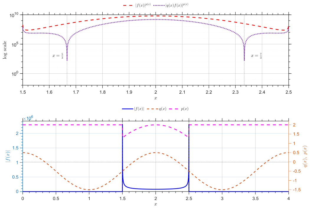
Figure 1 illustrates the mechanism by which the variable exponent restores integrability. The reduction of $p\left(x\right)$ near the singular endpoints $x=1.5$ and $x=2.5$ weakens the singularities of f at the modular level, yielding

$$f\in L^{p\left(x\right)}(0,\mathsf{\ell }).$$

Since $q\in L^{\infty }(0,\mathsf{\ell })$, it follows immediately that

$$qf\in L^{p\left(x\right)}(0,\mathsf{\ell }),$$

and therefore

$$f\in D\left(A\right),D\left(A\right)=\{g\in L^{p\left(x\right)}(0,\mathsf{\ell }):qg\in L^{p\left(x\right)}(0,\mathsf{\ell })\}.$$

The logarithmic scale used in the upper panel is particularly useful for visualizing the behavior of the modular densities over several orders of magnitude. It clearly reveals the local attenuation produced by the factor $q\left(x\right)$, as well as the pronounced minima occurring at the zeros of the multiplier,

$$x={\displaystyle \frac{5}{3}},x={\displaystyle \frac{7}{3}}.$$

By Theorem 3, the multiplication operator

$$A=M_q$$

is ${\rho }_{p(·)}$-closed, ${\rho }_{p(·)}$-densely defined, and bounded on $L^{p\left(x\right)}(0,\mathsf{\ell })$. Moreover,

$${\parallel A\parallel }_{\mathcal{L}(L^{p\left(x\right)}(0,\mathsf{\ell }))}={\parallel q\parallel }_{\infty }={\displaystyle \frac{3}{2}}.$$

We now examine the spectral properties of both the generator A and the associated semigroup $S\left(t\right)$. Since

$$q\left(x\right)=\cos \left(\pi (x-2)\right)-{\displaystyle \frac{1}{2}},$$

one has

$$-{\displaystyle \frac{3}{2}}\le q\left(x\right)\le {\displaystyle \frac{1}{2}},x\in (0,\mathsf{\ell }),$$

and both extremal values are attained. Hence,

$$\sigma \left(A\right)=\mathrm{ess}\hspace{0.17em}\mathrm{ran}\left(q\right)=\left[-{\displaystyle \frac{3}{2}},{\displaystyle \frac{1}{2}}\right].$$

For each $t>0$,

$$S\left(t\right)=M_{e^{tq}},$$

and therefore

$$\sigma \left(S\left(t\right)\right)=\mathrm{ess}\hspace{0.17em}\mathrm{ran}\left(e^{tq}\right)=e^{t\sigma \left(A\right)}=\left[e^{-3t/2},e^{t/2}\right].$$

Thus, the spectrum of the semigroup is obtained by exponentiating the spectrum of its generator.

The sign of $q\left(x\right)$ determines the local dynamics of the evolution. Regions where $q\left(x\right)<0$ correspond to exponential damping, whereas regions where $q\left(x\right)>0$ correspond to exponential amplification. The points

$$x={\displaystyle \frac{5}{3}},x={\displaystyle \frac{7}{3}},$$

separate these two regimes.

Finally, for $\lambda \notin \sigma \left(A\right)$, one has

$$(\lambda I-A)f=(\lambda -q)f,$$

so that

$$\lambda I-A=M_{\lambda -q}.$$

Since

$$\underset{x\in (0,\mathsf{\ell })}{\inf }|\lambda -q\left(x\right)|>0,$$

the inverse exists and is again a bounded multiplication operator,

$$R(\lambda ,A)={(\lambda I-A)}^{-1}=M_{1/(\lambda -q)},$$

that is,

$$\left(R(\lambda ,A)f\right)\left(x\right)={\displaystyle \frac{f\left(x\right)}{\lambda -q\left(x\right)}},f\in L^{p\left(x\right)}(0,\mathsf{\ell }).$$

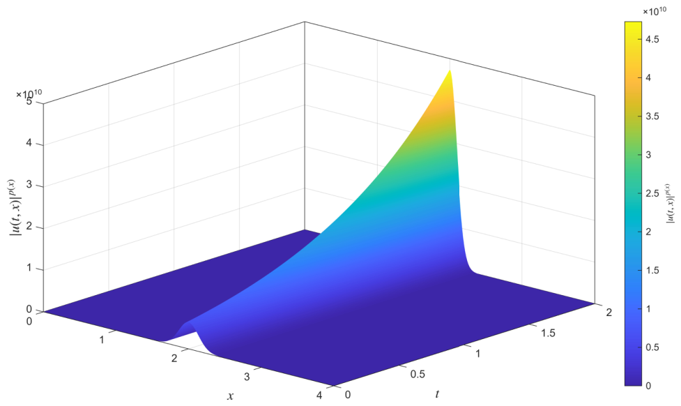
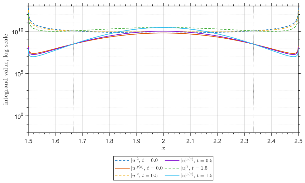
Figure 2 presents the semigroup evolution corresponding to a singular initial datum. The surface reflects the spatial dependence of the coefficient $q\left(x\right)$: regions corresponding to positive values of $q\left(x\right)$ exhibit amplification, whereas regions where $q\left(x\right)<0$ exhibit damping. This behavior is consistent with the spectral properties of the generator $A=M_q$ established above. The evolution preserves the principal characteristics of the initial datum, while its modular behavior remains governed by the variable exponent structure of the underlying space. Finally, we compare the classical fixed exponent density ${\left|u(t,x)\right|}^2$ with the variable exponent modular density ${\left|u(t,x)\right|}^{p\left(x\right)}$ on the active interval $(1.5,2.5).$

Figure 3 highlights the principal advantage of the variable exponent framework: while the fixed exponent density ${\left|u(t,x)\right|}^2$ remains large near the endpoints of the active interval, the modular density ${\left|u(t,x)\right|}^{p\left(x\right)}$ is significantly moderated by the local reduction of the exponent. The logarithmic representation is particularly useful because a linear scale would be dominated by the large values near the singularities and would conceal the behavior elsewhere in the interval. By contrast, the logarithmic scale allows one to visualize the attenuation effect produced by the variable exponent across the entire domain.

These results demonstrate how the variable exponent space $L^{p\left(x\right)}(0,\mathsf{\ell })$ accommodates singular initial data that are not admissible in the corresponding fixed exponent setting. The semigroup evolution preserves this property for all $t\ge 0,$ illustrating the effectiveness of the variable exponent framework for the analysis of evolution equations with localized singular behavior.

5. Discussion and Perspectives

The semigroup framework developed in this work provides a natural setting for the study of evolution equations in variable exponent Lebesgue spaces. In particular, strongly continuous semigroups acting on variable exponent Lebesgue spaces $L^{p\left(x\right)}(0,\mathsf{\ell })$ provide a natural framework for the analysis and approximation of abstract differential equations, delay equations, and nonlinear evolution problems with nonstandard growth conditions. The abstract formulation allows delay equations to be rewritten as Cauchy problems in suitable product spaces, making it possible to apply operator-theoretic techniques analogous to those developed in classical Banach spaces [1,2,3,4].

An important direction concerns approximation theory for evolution equations in variable exponent spaces. Finite-dimensional projections, Galerkin methods, averaging procedures, and operator-splitting techniques may potentially be extended to the modular framework. Similar approximation ideas for semilinear evolution equations and delay systems were studied in the classical setting in [18,19]. However, the extension of these methods to $L^{p\left(x\right)}$-spaces remains largely open due to the lack of translation invariance and the nonhomogeneous structure of the modular topology. In particular, the characterization of generators, spectral properties of unbounded operators, stability estimates, and convergence of approximation procedures in modular settings require further investigation.

More generally, modular techniques and variable growth conditions have recently played an important role in approximation theory, nonlinear operators, generalized function spaces, and functional analysis. In particular, modular methods and Steklov-type averaging operators have been employed in the study of approximation processes and neural network-type operators in generalized modular settings; see, for example, [14,15]. These developments further illustrate the flexibility of modular frameworks in the analysis of nonlinear and nonstandard growth phenomena.

The present framework also opens the possibility of studying delay differential equations with spatially varying regularity and integrability properties. Such models may be useful in applications where diffusion, memory, or response mechanisms vary spatially or temporally. Potential applications include heterogeneous biological systems, adaptive diffusion processes, electrorheological fluids, viscoelastic materials, and image restoration models with spatially dependent smoothing effects [6,7,9]. The flexibility of the exponent function $p\left(x\right)$ allows the local regularity of the phase space to adapt to the structure of the underlying problem, which cannot generally be captured within the classical fixed exponent $L^p$-framework.

Another interesting direction concerns the asymptotic behavior of semigroups in variable exponent spaces, including stability, bifurcation phenomena, periodic solutions, and attractor theory. The interaction between delay effects and variable growth conditions may generate new dynamical behaviors that do not appear in the classical setting. Extensions to Sobolev spaces with variable exponents, unbounded domains, transport equations, and nonlinear semigroup settings also remain important open problems for future research.

The multiplication semigroups studied in the present work therefore provide a first step toward a broader semigroup theory in variable exponent spaces and suggest several directions for the future for numerics and real-life applications.