On a New Subclass of Multivalent Harmonic Mappings Associated with Close-to-Convex Functions

Abstract

This paper is devoted to defining and analyzing a new subclass $M(\nu ,\tau ,q)$ of q-valent harmonic mappings in the unit disk D, as well as investigating its connection with close-to-convex analytic functions. First, we prove that this newly defined class is non-empty and discuss its relationship with several known classes of harmonic mappings. Using arguments similar to those employed in the study of Mocanu-type harmonic mappings, we establish the close-to-convexity of functions belonging to this class. Necessary coefficient estimates for the analytic part are obtained, and auxiliary lemmas which play an essential role in the investigation of geometric properties of the class are derived. In particular, we establish distortion estimates for the derivative of the analytic part, which lead to a growth and distortion theorem for functions in the newly defined class $M(\nu ,\tau ,q)$. Furthermore, a covering theorem is obtained for these harmonic mappings. In addition, we also derive sharp bounds for the Fekete–Szegö-type functionals and several graphical examples are presented to analyze the geometric structure of the mappings in the class $M(\nu ,\tau ,q)$ that demonstrate how the parameters $q,\nu ,$ and $\tau ,$ affect the deformation of the unit disk.

1. Introduction

Let $\mathcal{A}$ denote the class of analytic functions in D normalized by the series

$$f\left(\vartheta \right)=\vartheta +{\displaystyle \sum _{k=2}^{\infty }}{a}_k{\vartheta }^k.$$

A function $f\in \mathcal{A}$ is said to be univalent if it is one-to-one in D, and the subclass of univalent functions is represented by $\mathcal{S}$. Important subclasses of $\mathcal{S}$ are starlike, convex and close-to-convex functions. These classes have been extensively studied due to their strong geometric properties.

Harmonic mappings in the complex plane gain substantial attention in geometric function theory (GFT) because of their abundant geometric structure and numerous applications. A complex-valued harmonic function $\phi$ can be formulated as

$$\phi =l+\overline{m},$$

(1)

where

$$l\left(\vartheta \right)=\vartheta +{\displaystyle \sum _{k=2}^{\infty }}{a}_k{\vartheta }^k,m\left(\vartheta \right)={\displaystyle \sum _{k=1}^{\infty }}{b}_k{\vartheta }^k$$

(2)

are analytic and co-analytic functions in the open unit disk

$$D=\{\vartheta \in \mathbb{C}:|\vartheta |<1\}.$$

A harmonic mapping (HMp) is called sense-preserving and locally univalent in D if the Jacobian

$$J_{\phi }\left(\vartheta \right)=|l^{\prime }{\left(\vartheta \right)|}^2-{\left|m^{\prime }\left(\vartheta \right)\right|}^2$$

is positive in D (see Clunie and Sheil-Small [1] and Duren [2]). The study of geometric characteristics of HMp such as univalence, starlikeness, convexity and close-to-convexity are the hot topic of research for the last few years.

One of the classical problems in GFT is the Fekete–Szegö problem [3], which concerns sharp bounds of the nonlinear functional $|a_3-\lambda a_2^2|$ for functions belonging to various subclasses of $\mathcal{S}$. This problem has been widely investigated for many analytic and harmonic function classes (see [4,5,6]).

In the context of harmonic mappings, several subclasses associated with convex and close-to-convex functions have been introduced and studied. In particular, Mocanu [7] introduced a class of harmonic mappings satisfying certain differential conditions, and conjectures of the functions in the family $M(1,-\frac{1}{2},1)$ are univalent in D. These conjectures were later confirmed by Bshouty and Lyzzaik [8] who showed that

$$M(1,-\frac{1}{2},1)\subset C_H^0,$$

where $C_H^0$ denotes the class of close-to-convex HMp. Further investigations and extensions of these results can be found in [9,10,11,12,13]. Recent investigations on subclasses of harmonic mappings and their geometric properties have been carried out by several authors. In particular, Arif et al. [14,15,16] studied subclasses of harmonic close-to-convex mappings connected with Janowski functions and found coefficient estimates and Fekete–Szegö inequalities. Li and Ponnusamy [17,18] investigated coefficient bounds and subordination conditions for various harmonic mappings, while Wang et al. [19] and Chen et al. [10] studied differential operators and radius problems for harmonic mappings. For more recent studies see [20,21,22,23,24]. These results demonstrate that the investigation of subclasses of harmonic mappings and their coefficient problems remains an active area of research in GFT.

1.1. Motivation and Contribution

The study of harmonic mappings has attained notable attention in recent years due to their rich geometric behavior and vast applicability in complex analysis, fluid dynamics, and some related fields. Specifically, subclasses of harmonic mappings connected with convexity, starlikeness, and close-to-convexity have been thoroughly investigated because of their strong geometric structure and connections with the theory of univalent functions. On the other hand, multivalent (q-valent) analytic functions gave a natural generalization of univalent functions and have been proven to exhibit more complex geometric behavior. However, the corresponding theory for multivalent harmonic mappings is still comparatively less developed, especially in the framework of close-to-convexity and controlled dilatation. It is natural to determine and study new subclasses of harmonic mappings that simultaneously include multivalency, geometric constraints on the analytic part, and explicit control over the dilatation. This offers a more flexible framework for extending classical results and obtaining sharper geometric bounds. Motivated by these developments, we discuss and analyze a new subclass of harmonic mappings related with multivalent close-to-convex functions. The class $M(\nu ,\tau ,q)$ can be regarded as a harmonic extension of the analytic class of q-valent convex functions of order $\tau$. The main contributions of this article are summarized as follows:

• We introduce a new subclass $M(\nu ,\tau ,q)$ of q-valent harmonic mappings associated with close-to-convex analytic functions and show that this class is non-empty.
• We discuss the relationship between the class $M(\nu ,\tau ,q)$ and several previously studied subclasses of harmonic mappings and establish the close-to-convexity of functions belonging to this class.
• We obtain coefficient estimates for the analytic and co-analytic parts of functions in the class $M(\nu ,\tau ,q)$.
• We establish auxiliary lemmas for functions in the analytic class $K(\tau ,q)$, as they are essential in deriving the geometric properties of the new class.
• Using these lemmas, we derive a growth and distortion theorem for functions in the class $M(\nu ,\tau ,q)$.
• A covering theorem which describes the image of the unit disk under mappings belonging to this class is obtained.
• Also, we obtain bounds for the Fekete–Szegö-type functionals $|a_{q+2}-\lambda a_{q+1}^2|$ and $|b_{q+2}-\lambda b_{q+1}^2|$.

Definition 1.

Let $q\in \mathbb{N}$, $\nu \in \mathbb{C}$ with $\left|\nu \right|\le 1$, and $-{\displaystyle \frac{1}{2}}\le \tau <1$. A harmonic function φ defined in $D=\{\vartheta \in \mathbb{C}:|\vartheta |<1\}$ is said to belong to the class $M(\nu ,\tau ,q)$ if

$$\phi \left(\vartheta \right)=l\left(\vartheta \right)+\overline{m\left(\vartheta \right)},$$

(3)

where l is analytic and m is co-analytic in D, and both have the series representations

$$l\left(\vartheta \right)={\vartheta }^q+{\displaystyle \sum _{k=2}^{\infty }}{a}_{k+q-1}{\vartheta }^{k+q-1},m\left(\vartheta \right)={\displaystyle \sum _{k=1}^{\infty }}{b}_{k+q-1}{\vartheta }^{k+q-1},\left|b_q\right|<1.$$

(4)

Furthermore, the functions l and m satisfy the conditions

$$m^{\prime }\left(\vartheta \right)={\displaystyle \frac{\nu }{q}}{l}^{\prime }\left(\vartheta \right),$$

(5)

and

$$\Re \left(1+{\displaystyle \frac{\vartheta l^{″}\left(\vartheta \right)}{q{l}^{\prime }\left(\vartheta \right)}}\right)>\tau ,\vartheta \in D.$$

(6)

Remark 1.

We note that the class $M(\nu ,\tau ,q)$ is well-defined and mathematically consistent. Indeed, a harmonic mapping $\phi =l+\overline{m}$ in the unit disk D is locally univalent and sense-preserving if and only if its dilatation

$$\omega \left(\vartheta \right)={\displaystyle \frac{m^{\prime }\left(\vartheta \right)}{l^{\prime }\left(\vartheta \right)}}$$

satisfies $\left|\omega \right(\vartheta \left)\right|<1$ for $\vartheta \in D$ (see [1,2]). For functions in the class $M(\nu ,\tau ,q)$, the relation

$$m^{\prime }\left(\vartheta \right)={\displaystyle \frac{\nu }{q}}{l}^{\prime }\left(\vartheta \right)$$

implies that the dilatation is constant and given by

$$\omega \left(\vartheta \right)={\displaystyle \frac{\nu }{q}}.$$

Since $\left|\nu \right|\le 1$ and $q\ge 1$, it means that $\left|\omega \right(\vartheta \left)\right|\le 1/q<1$, and hence φ is sense-preserving in D.

Moreover, the condition

$$\Re \left(1+{\displaystyle \frac{\vartheta l^{″}\left(\vartheta \right)}{q{l}^{\prime }\left(\vartheta \right)}}\right)>\tau ,-{\displaystyle \frac{1}{2}}\le \tau <1,$$

is a natural extention of the analytic class of convex functions of order τ to the q-valent setting. In particular, this condition ensures that the analytic part l is in the class of q-valent convex functions of order τ. Consequently, the harmonic mapping φ inherits geometric properties closely related to close-to-convexity and univalence. Therefore, the class $M(\nu ,\tau ,q)$ provides a consistent framework for studying q-valent harmonic mappings with controlled dilatation and convexity conditions on the analytic part.

Proposition 1.

The class $M(\nu ,\tau ,q)$ is non-empty.

Proof. 

To show that the class $M(\nu ,\tau ,q)$ is non-empty, it is sufficient to construct a harmonic mapping $\phi =l+\overline{m}$ that satisfies the defining conditions of the class.

Consider the analytic function

$$l\left(\vartheta \right)={\vartheta }^q,\vartheta \in D.$$

Then

$$l^{\prime }\left(\vartheta \right)=q{\vartheta }^{q-1},l^{″}\left(\vartheta \right)=q(q-1){\vartheta }^{q-2}.$$

Now compute

$$1+{\displaystyle \frac{\vartheta l^{″}\left(\vartheta \right)}{q{l}^{\prime }\left(\vartheta \right)}}.$$

Substituting the derivatives, we obtain

$$1+{\displaystyle \frac{\vartheta q(q-1){\vartheta }^{q-2}}{q\left(q{\vartheta }^{q-1}\right)}}=1+{\displaystyle \frac{q-1}{q}}.$$

Thus

$$1+{\displaystyle \frac{\vartheta l^{″}\left(\vartheta \right)}{q{l}^{\prime }\left(\vartheta \right)}}=2-{\displaystyle \frac{1}{q}}.$$

Since $q\ge 1$, we have

$$2-{\displaystyle \frac{1}{q}}>1.$$

Therefore

$$\Re \left(1+{\displaystyle \frac{\vartheta l^{″}\left(\vartheta \right)}{q{l}^{\prime }\left(\vartheta \right)}}\right)=2-{\displaystyle \frac{1}{q}}>\tau ,$$

because $-{\displaystyle \frac{1}{2}}\le \tau <1$. Hence the analytic part satisfies the required convexity-type condition.

Construction of the co-analytic part:

From the definition of $M(\nu ,\tau ,q)$ we require

$$m^{\prime }\left(\vartheta \right)={\displaystyle \frac{\nu }{q}}\vartheta l^{\prime }\left(\vartheta \right),\left|\nu \right|\le 1.$$

Since

$$\vartheta l^{\prime }\left(\vartheta \right)=q{\vartheta }^q,$$

we obtain

$$m^{\prime }\left(\vartheta \right)=\nu {\vartheta }^q.$$

(7)

Integrating this, we obtain

$$m\left(\vartheta \right)={\displaystyle \frac{\nu }{q+1}}{\vartheta }^{q+1},$$

where the constant of integration is taken as zero so that $m\left(0\right)=0$.

Verification of the harmonic mapping:

Define

$$\phi \left(\vartheta \right)=l\left(\vartheta \right)+\overline{m\left(\vartheta \right)}={\vartheta }^q+\overline{\left({\displaystyle \frac{\nu }{q+1}}{\vartheta }^{q+1}\right)}.$$

The dilatation of $\phi$ is

$$\omega \left(\vartheta \right)={\displaystyle \frac{m^{\prime }\left(\vartheta \right)}{l^{\prime }\left(\vartheta \right)}}={\displaystyle \frac{\nu {\vartheta }^q}{q{\vartheta }^{q-1}}}={\displaystyle \frac{\nu \vartheta }{q}}.$$

Hence

$$\left|\omega \left(\vartheta \right)\right|=\left|{\displaystyle \frac{\nu \vartheta }{q}}\right|\le {\displaystyle \frac{1}{q}}<1,$$

because $\left|\nu \right|\le 1$, $\left|\vartheta \right|<1$ and $q\ge 1$. Therefore $\phi$ is sense-preserving in D.

Therefore harmonic mapping

$$\phi \left(\vartheta \right)={\vartheta }^q+\overline{\left({\displaystyle \frac{\nu }{q+1}}{\vartheta }^{q+1}\right)}$$

satisfies all defining conditions of the class $M(\nu ,\tau ,q)$. Hence the class $M(\nu ,\tau ,q)$ contains at least one function and therefore is non-empty. □

Remark 2

(Special cases of the class $M(\nu ,\tau ,q)$). Several well-known subclasses of harmonic mappings arise as special cases of the class $M(\nu ,\tau ,q)$.

1. 

If $q=1$, then the class $M(\nu ,\tau ,q)$ reduces to the class $M(\nu ,\tau )$ (see [25]) of harmonic mappings satisfying

$$m^{\prime }\left(\vartheta \right)=\nu \vartheta l^{\prime }\left(\vartheta \right),\Re \left(1+{\displaystyle \frac{\vartheta l^{″}\left(\vartheta \right)}{l^{\prime }\left(\vartheta \right)}}\right)>\tau .$$

2. 

If $q=1$ and $\tau =-{\displaystyle \frac{1}{2}}$, we obtain the class $M(\nu ,-\frac{1}{2},1)$ (see [7]).

3. 

It is known that (see [8])

$$M(1,-\frac{1}{2},1)\subset C_H^0.$$

4. 

More generally (see [9]),

$$M(\nu ,-\frac{1}{2},1)\subset C_H^0\mathrm{for}\left|\nu \right|=1.$$

5. 

Furthermore, Nagpal and Ravichandran [12] proved that

$$M(1,-\frac{1}{2},1)\not\subset S_H^{0,*}.$$

and also studied new results

$$M(1,-\frac{1}{2},1)$$

for $\left|\nu \right|=1$.

Remark 3

(Relationship with known classes). The class $M(\nu ,\tau ,q)$ is closely related to several well-known subclasses of harmonic mappings. In particular,

$$M(\nu ,\tau ,q)\subset M\left(\nu ,-\frac{1}{2},1\right).$$

Furthermore,

$$M\left(\nu ,-\frac{1}{2},1\right)\subset C_H^0.$$

Consequently,

$$M(\nu ,\tau ,q)\subset M\left(\nu ,-\frac{1}{2},1\right)\subset C_H^0\subset S_H$$

1.2. Novelty

In this paper, we introduce and analyze a new subclass $M(\nu ,\tau ,q)$ of q-valent harmonic mappings related with close-to-convex functions in the open unit disk. The distinctive feature of this class is the integrated incorporation of three essential aspects: the q-valent structure, a parameter-dependent dilatation determined by $\nu$, and a convexity-type condition of order $\tau$ applied on the analytic part.

This approach provides a systematic method for studying multivalent harmonic mappings with explicitly controlled geometric behavior. Therefore, we obtain several new and refined results, including sharp coefficient estimates, Fekete–Szegö-type inequalities, as well as growth, distortion, and covering theorems. Moreover, the corresponding extremal functions are explicitly constructed, and the theoretical results are supported by graphical visualizations that determine the geometric deformation of the unit disk under the mappings. These findings extend existing results in the literature and offer a consistent foundation for further developments in geometric function theory.

2. Set of Lemmas

Lemma 1

([1], Lemma 5.15). Suppose l and m are analytic in U with $|l^{\prime }\left(0\right)|<|m^{\prime }\left(0\right)|$ and $F_{\mu }=l+\mu m$ is close-to-convex for each μ$\left(\right|\mu |=1)$; then $\phi =l+m$ is close-to-convex in U.

Lemma 2

(Carathéodory lemma [2,26]). If $p\left(\vartheta \right)$ is analytic in D, $p\left(0\right)=1$, and $\Re \left(p\right(\vartheta \left)\right)>0$, then for $n\ge 1$,

$$|c_n|\le 2$$

and

$$|c_2-\mu c_1^2|\le 2max\{1,|1-2\mu |\}.$$

Lemma 3

([27], (Formula (10))). Let

$$p\left(\vartheta \right)=1+{\displaystyle \sum _{k=1}^{\infty }}{c}_k{\vartheta }^k$$

(8)

be an analytic function in the unit disk $\mathbb{D}$ satisfying

$$\Re \left(p\left(\vartheta \right)\right)>0,\vartheta \in \mathbb{D}.$$

(9)

Then, the coefficients satisfy

$$\left|c_2-{\displaystyle \frac{c_1^2}{2}}\right|\le 2-{\displaystyle \frac{|c_1{|}^2}{2}}.$$

(10)

Lemma 4

((Logarithmic-derivative distortion estimate; see, e.g., [27,28])). If F is analytic in D, $F\left(0\right)=1$, and

$$\Re \left({\displaystyle \frac{\vartheta F^{\prime }\left(\vartheta \right)}{F\left(\vartheta \right)}}\right)>-\alpha (\alpha >0),$$

then for $\left|\vartheta \right|=r<1$,

$${\displaystyle \frac{1}{{(1+r)}^{\alpha }}}\le \left|F\left(\vartheta \right)\right|\le {\displaystyle \frac{1}{{(1-r)}^{\alpha }}}.$$

3. Main Results

3.1. Close-to-Convexity

Theorem 1.

Let $\phi =l+\overline{m}$ belong to the class $M(\nu ,\tau ,q)$. Then φ is close-to-convex in the unit disk D. Consequently,

$$M(\nu ,\tau ,q)\subset C_H.$$

Proof. 

Let $\phi =l+\overline{m}\in M(\nu ,\tau ,q)$. Then by definition we have

$$m^{\prime }\left(\vartheta \right)={\displaystyle \frac{\nu }{q}}\vartheta l^{\prime }\left(\vartheta \right),\left|\nu \right|\le 1,$$

and

$$\Re \left(1+{\displaystyle \frac{\vartheta l^{″}\left(\vartheta \right)}{q{l}^{\prime }\left(\vartheta \right)}}\right)>\tau ,-{\displaystyle \frac{1}{2}}\le \tau <1.$$

Property of the analytic part:

The condition

$$\Re \left(1+{\displaystyle \frac{\vartheta l^{″}\left(\vartheta \right)}{q{l}^{\prime }\left(\vartheta \right)}}\right)>\tau$$

implies that the analytic function l belongs to the class of q-valent convex functions of order $\tau$. It is known that such functions are close-to-convex in D.

Construction of auxiliary functions:

For any complex number $\mu$ with $\left|\mu \right|=1$, consider

$$F_{\mu }\left(\vartheta \right)=l\left(\vartheta \right)+\mu m\left(\vartheta \right).$$

By differentiating it, we obtain

$$F_{\mu }^{\prime }\left(\vartheta \right)=l^{\prime }\left(\vartheta \right)+\mu m^{\prime }\left(\vartheta \right).$$

Using the relation $m^{\prime }\left(\vartheta \right)={\displaystyle \frac{\nu }{q}}\vartheta l^{\prime }\left(\vartheta \right)$, we obtain

$$F_{\mu }^{\prime }\left(\vartheta \right)=l^{\prime }\left(\vartheta \right)\left(1+{\displaystyle \frac{\mu \nu \vartheta }{q}}\right).$$

Close-to-convexity of ${\mathbf{F}}_{\mathbf{\mu }}$:

Since $\left|\mu \right|=1$ and $\left|\nu \right|\le 1$, it follows that

$$\left|{\displaystyle \frac{\mu \nu \vartheta }{q}}\right|\le {\displaystyle \frac{1}{q}}<1.$$

Thus the factor $\left(1+{\displaystyle \frac{\mu \nu \vartheta }{q}}\right)$ never vanishes in D. Therefore

$$F_{\mu }^{\prime }\left(\vartheta \right)\ne 0$$

whenever $l^{\prime }\left(\vartheta \right)\ne 0$. Since l is close-to-convex, it follows that $F_{\mu }$ is also close-to-convex in D.

Using Lemma 1 we conclude that $\phi$ is close-to-convex.

Hence

$$M(\nu ,\tau ,q)\subset C_H.$$

This completes the proof. □

The following lemma is very necessary to prove the nth coefficients’ inequalities for the function $\phi =l+m\in M(\nu ,\tau ,q)$.

Lemma 5.

Let $l\left(\vartheta \right)\in K(\tau ,q)$ with the series representation

$$l\left(\vartheta \right)={\vartheta }^q+{\displaystyle \sum _{k=2}^{\infty }}{a}_{k+q-1}{\vartheta }^{k+q-1},-{\displaystyle \frac{1}{2}}\le \tau <1,q\in \mathbb{N}.$$

Then, for $k\ge 2$,

$$|a_{k+q-1}|\le {\displaystyle \frac{1}{(k+q-1)}}·{\displaystyle \frac{{\left(2q(1-\tau )\right)}_{k-1}}{(k-1)!}}.$$

(11)

The estimate is sharp. Equality holds for the extremal function

$$l\left(\vartheta \right)={\int }_0^{\vartheta }{\displaystyle \frac{t^{q-1}}{{(1-\gamma t)}^{2q(1-\tau )}}}dt,\left|\gamma \right|=1.$$

Proof. 

Since $l\in K(\tau ,q)$, we have

$$\Re \left(1+{\displaystyle \frac{\vartheta l^{″}\left(\vartheta \right)}{q{l}^{\prime }\left(\vartheta \right)}}\right)>\tau ,\vartheta \in U.$$

Hence there exists a function $p\left(\vartheta \right)$ analytic in U with $p\left(0\right)=1$ and $\Re \left(p\right(\vartheta \left)\right)>0$ such that

$$1+{\displaystyle \frac{\vartheta l^{″}\left(\vartheta \right)}{q{l}^{\prime }\left(\vartheta \right)}}=\tau +(1-\tau )p\left(\vartheta \right).$$

Thus

$${\displaystyle \frac{\vartheta l^{″}\left(\vartheta \right)}{l^{\prime }\left(\vartheta \right)}}=q(1-\tau )\left(p\left(\vartheta \right)-1\right),$$

or

$${\displaystyle \frac{l^{″}\left(\vartheta \right)}{l^{\prime }\left(\vartheta \right)}}={\displaystyle \frac{q(1-\tau )}{\vartheta }}\left(p\left(\vartheta \right)-1\right).$$

By integrating it, we obtain

$$log{l}^{\prime }\left(\vartheta \right)=q(1-\tau ){\int }_0^{\vartheta }{\displaystyle \frac{p\left(t\right)-1}{t}}dt.$$

For the extremal case, take

$$p\left(\vartheta \right)={\displaystyle \frac{1+\gamma \vartheta }{1-\gamma \vartheta }},\left|\gamma \right|=1.$$

Then

$${\displaystyle \frac{p\left(\vartheta \right)-1}{\vartheta }}={\displaystyle \frac{2\gamma }{1-\gamma \vartheta }}.$$

Hence

$$log{l}^{\prime }\left(\vartheta \right)=2q(1-\tau ){\int }_0^{\vartheta }{\displaystyle \frac{\gamma }{1-\gamma t}}dt=-2q(1-\tau )log(1-\gamma \vartheta ).$$

Therefore

$$l^{\prime }\left(\vartheta \right)={\displaystyle \frac{{\vartheta }^{q-1}}{{(1-\gamma \vartheta )}^{2q(1-\tau )}}}.$$

After integrating it, we obtain

$$l\left(\vartheta \right)={\int }_0^{\vartheta }{\displaystyle \frac{t^{q-1}}{{(1-\gamma t)}^{2q(1-\tau )}}}dt.$$

Now expand

$${(1-\gamma t)}^{-2q(1-\tau )}={\displaystyle \sum _{n=0}^{\infty }}{\displaystyle \frac{{\left(2q(1-\tau )\right)}_n}{n!}}{\gamma }^n{t}^n.$$

Thus

$$l^{\prime }\left(\vartheta \right)={\displaystyle \sum _{n=0}^{\infty }}{\displaystyle \frac{{\left(2q(1-\tau )\right)}_n}{n!}}{\gamma }^n{\vartheta }^{n+q-1}.$$

Integrating term by term gives

$$l\left(\vartheta \right)={\displaystyle \sum _{n=0}^{\infty }}{\displaystyle \frac{{\left(2q(1-\tau )\right)}_n}{n!(n+q)}}{\gamma }^n{\vartheta }^{n+q}.$$

Hence

$$a_{k+q-1}={\displaystyle \frac{{\left(2q(1-\tau )\right)}_{k-1}}{(k-1)!(k+q-1)}}{\gamma }^{k-1}.$$

This proves the result. □

Corollary 1

([29]). Let $l\left(\vartheta \right)\in K(\tau ,1)$ with

$$l\left(\vartheta \right)=\vartheta +{\displaystyle \sum _{k=2}^{\infty }}{a}_k{\vartheta }^k,-{\displaystyle \frac{1}{2}}\le \tau <1.$$

Then

$$|a_k|\le {\displaystyle \frac{{\left(2(1-\tau )\right)}_{k-1}}{k!}}={\displaystyle \frac{1}{k!}}{\displaystyle \prod _{j=2}^k}(j-2\tau ).$$

The estimate is sharp.

By comparing the coefficients of similar powers of $\vartheta$ in the identity $m^{\prime }\left(\vartheta \right)=\nu \vartheta l^{\prime }\left(\vartheta \right)$, we obtain

$$(k+q)b_{k+q}=(k+q-1)\nu a_{k+q-1},k\ge 1.$$

Now, we discuss the coefficient estimates involving functions of the class $M(\nu ,\tau ,q)$. In view of this observation and the known estimate for $|a_{k+q-1}|$ in Lemma 5, we obtain the following result.

Theorem 2.

Let $\phi =l+m\in M(\nu ,\tau ,q)$ be of Form (3). Then for $k\ge 2$,

$$|a_{k+q-1}|\le {\displaystyle \frac{1}{(k+q-1)}}·{\displaystyle \frac{{\left(2q(1-\tau )\right)}_{k-1}}{(k-1)!}}.$$

(12)

$$|b_{q+1}|\le {\displaystyle \frac{\nu q}{q+1}},$$

and

$$|b_{k+q}|\le {\displaystyle \frac{\left|\nu \right|}{k+q}}·{\displaystyle \frac{{\left(2q(1-\tau )\right)}_{k-1}}{(k-1)!}}.$$

Moreover, the bounds are sharp and are attained by the extremal harmonic mappings

$${\phi }_{\nu ,\tau ,q}\left(\vartheta \right)={\int }_0^{\vartheta }{\displaystyle \frac{dt}{{(1-\gamma t)}^{2q(1-\tau )}}}+\overline{{\displaystyle \frac{\nu }{q}}{\int }_0^{\vartheta }{\displaystyle \frac{tdt}{{(1-\gamma t)}^{2q(1-\tau )}}}},\left|\gamma \right|=1,\vartheta \in D.$$

Corollary 2

([25]). Let $\phi =l+m\in M(\nu ,\tau ,1)$ be of Form (3). Then for $k\ge 2$,

$$|a_k|\le {\displaystyle \frac{1}{k!}}{\displaystyle \prod _{j=2}^k}(j-2\tau ).$$

(13)

$$b_2={\displaystyle \frac{\nu }{2}},$$

and

$$|b_k|\le {\displaystyle \frac{(k-1)|\nu |}{\left(k\right)!}}{\displaystyle \prod _{j=2}^{k-1}}(j-2\tau ).$$

Moreover, the bounds are sharp and are attained by the extremal harmonic mappings

$${\phi }_{\nu ,\tau ,1}\left(\vartheta \right)={\int }_0^{\vartheta }{\displaystyle \frac{dt}{{(1-\gamma t)}^{2(1-\tau )}}}+\overline{{\displaystyle \frac{\nu }{1}}{\int }_0^{\vartheta }{\displaystyle \frac{tdt}{{(1-\gamma t)}^{2(1-\tau )}}}},\left|\gamma \right|=1,\vartheta \in D.$$

Example 1.

Let $q=2$, $\tau ={\displaystyle \frac{1}{2}}$, and $\nu ={\displaystyle \frac{1}{2}}$. Then the extremal mapping becomes

$$\phi \left(\vartheta \right)={\int }_0^{\vartheta }{\displaystyle \frac{dt}{{(1-t)}^3}}+\overline{{\displaystyle \frac{1}{4}}{\int }_0^{\vartheta }{\displaystyle \frac{tdt}{{(1-t)}^3}}}.$$

Example 2.

Let $\phi =l+m\in M(\nu ,\tau ,q)$ with parameters

$$q=2,\tau ={\displaystyle \frac{1}{2}},\nu ={\displaystyle \frac{1}{2}}.$$

Consider the extremal mapping

$${\phi }_{\nu ,\tau }\left(\vartheta \right)={\int }_0^{\vartheta }{\displaystyle \frac{dt}{{(1-t)}^{2(q-\tau )}}}+\overline{{\displaystyle \frac{\nu }{q}}{\int }_0^{\vartheta }{\displaystyle \frac{dt}{{(1-t)}^{2(q-\tau )}}}}.$$

For $q=2$ and $\tau ={\displaystyle \frac{1}{2}}$ we obtain

$$\phi \left(\vartheta \right)={\int }_0^{\vartheta }{\displaystyle \frac{dt}{{(1-t)}^3}}+\overline{{\displaystyle \frac{1}{4}}{\int }_0^{\vartheta }{\displaystyle \frac{dt}{{(1-t)}^3}}}.$$

Since

$${\int }_0^{\vartheta }{\displaystyle \frac{dt}{{(1-t)}^3}}={\displaystyle \frac{1}{2}}\left({\displaystyle \frac{1}{{(1-\vartheta )}^2}}-1\right),$$

the extremal mapping becomes

$$\phi \left(\vartheta \right)={\displaystyle \frac{1}{2}}\left({\displaystyle \frac{1}{{(1-\vartheta )}^2}}-1\right)+\overline{{\displaystyle \frac{1}{8}}\left({\displaystyle \frac{1}{{(1-\vartheta )}^2}}-1\right)}.$$

Example 3.

Let $\phi =l+m\in M(\nu ,-{\displaystyle \frac{1}{2}},q)$ be of Form (3). Then

$$|a_{k+q-1}|\le {\displaystyle \frac{k+q}{2}},(k=3,4,\dots ),$$

and

$$|b_{k+q-1}|\le {\displaystyle \frac{(k+q-2)|\nu |}{2}},(k=3,4,\dots ).$$

For $q=1$, one gets the following inequality.

Example 4.

Let $\phi =l+m\in M(\nu ,-{\displaystyle \frac{1}{2}},q)$ be of Form (3). Then

$$|a_k|\le {\displaystyle \frac{k+1}{2}},$$

and

$$|b_{k+q-1}|\le {\displaystyle \frac{(k-1)|\nu |}{2}},(k=3,4,\dots ).$$

The results are sharp with the extremal functions

$${\phi }_{\nu ,-{\displaystyle \frac{1}{2}}}\left(\vartheta \right)={\displaystyle \frac{1}{2}}\left({\displaystyle \frac{\vartheta }{{(1-\gamma \vartheta )}^2}}+{\displaystyle \frac{\vartheta }{1-\gamma \vartheta }}\right)+{\displaystyle \frac{\nu }{2\gamma }}\left({\displaystyle \frac{\vartheta }{{(1-\gamma \vartheta )}^2}}-{\displaystyle \frac{\vartheta }{1-\gamma \vartheta }}\right),\left|\gamma \right|=1,\vartheta \in D.$$

3.2. Fekete–Szegö Functionals

Now, we give upper bounds for the Fekete–Szegö functionals

$$|a_{q+2}-\lambda a_{q+1}^2|\mathrm{and}|b_{q+2}-\lambda b_{q+1}^2|$$

for the functions in the class $M(\nu ,\tau ,q)$.

Theorem 3.

Let $\phi =l+m\in M(\nu ,\tau ,q)$ be of Form (3). Then

$$|a_{q+2}-\lambda a_{q+1}^2|\le {\displaystyle \frac{q(1-\tau )}{q+2}}max\left\{1,\left|1+2(1-\tau )\left(1-{\displaystyle \frac{2q(q+2)}{{(q+1)}^2}}\lambda \right)\right|\right\}.$$

(14)

Furthermore,

$$|b_{q+2}-\lambda b_{q+1}^2|\le {\displaystyle \frac{|\nu |(1-\tau )}{q+2}}+{\displaystyle \frac{{4|\nu |}^2{(1-\tau )}^2}{{(q+1)}^2}}|\lambda |.$$

(15)

Proof. 

Since $\phi \in M(\nu ,\tau ,q)$, the analytic part l satisfies

$$\Re \left(1+{\displaystyle \frac{\vartheta l^{″}\left(\vartheta \right)}{q{l}^{\prime }\left(\vartheta \right)}}\right)>\tau .$$

Hence there exists an analytic function $p\left(\vartheta \right)$ with $p\left(0\right)=1$ and $\Re \left(p\right(\vartheta \left)\right)>0$ such that

$$1+{\displaystyle \frac{\vartheta l^{″}\left(\vartheta \right)}{q{l}^{\prime }\left(\vartheta \right)}}=\tau +(1-\tau )p\left(\vartheta \right).$$

Let

$$p\left(\vartheta \right)=1+c_1\vartheta +c_2{\vartheta }^2+\cdots .$$

Thus

$$1+{\displaystyle \frac{\vartheta l^{″}\left(\vartheta \right)}{q{l}^{\prime }\left(\vartheta \right)}}=1+(1-\tau )c_1\vartheta +(1-\tau )c_2{\vartheta }^2+\cdots .$$

Now consider

$$l\left(\vartheta \right)={\vartheta }^q+a_{q+1}{\vartheta }^{q+1}+a_{q+2}{\vartheta }^{q+2}+\cdots .$$

Then

$$l^{\prime }\left(\vartheta \right)=q{\vartheta }^{q-1}+(q+1)a_{q+1}{\vartheta }^q+(q+2)a_{q+2}{\vartheta }^{q+1}+\cdots ,$$

$$l^{″}\left(\vartheta \right)=q(q-1){\vartheta }^{q-2}+q(q+1)a_{q+1}{\vartheta }^{q-1}+(q+1)(q+2)a_{q+2}{\vartheta }^q+\cdots .$$

Multiplying by $\vartheta$ yields

$$\vartheta l^{″}\left(\vartheta \right)=q(q-1){\vartheta }^{q-1}+q(q+1)a_{q+1}{\vartheta }^q+(q+1)(q+2)a_{q+2}{\vartheta }^{q+1}+\cdots .$$

Now compute

$$1+{\displaystyle \frac{\vartheta l^{″}\left(\vartheta \right)}{q{l}^{\prime }\left(\vartheta \right)}}={\displaystyle \frac{q{l}^{\prime }\left(\vartheta \right)+\vartheta l^{″}\left(\vartheta \right)}{q{l}^{\prime }\left(\vartheta \right)}}.$$

After simplification, we obtain

$$1+{\displaystyle \frac{\vartheta l^{″}\left(\vartheta \right)}{q{l}^{\prime }\left(\vartheta \right)}}=1+{\displaystyle \frac{q+1}{q}}{a}_{q+1}\vartheta +\left({\displaystyle \frac{2(q+2)}{q}}{a}_{q+2}-{\displaystyle \frac{{(q+1)}^2}{q^2}}{a}_{q+1}^2\right){\vartheta }^2+\cdots .$$

Comparing coefficients gives

$${\displaystyle \frac{q+1}{q}}{a}_{q+1}=(1-\tau )c_1,a_{q+1}={\displaystyle \frac{q}{q+1}}(1-\tau )c_1.$$

Similarly,

$${\displaystyle \frac{2(q+2)}{q}}{a}_{q+2}-{\displaystyle \frac{{(q+1)}^2}{q^2}}{a}_{q+1}^2=(1-\tau )c_2.$$

Hence

$$a_{q+2}={\displaystyle \frac{q(1-\tau )}{2(q+2)}}\left(c_2+(1-\tau )c_1^2\right).$$

Now

$$a_{q+2}-\lambda a_{q+1}^2={\displaystyle \frac{q(1-\tau )}{2(q+2)}}\left(c_2+(1-\tau )c_1^2\right)-\lambda {\displaystyle \frac{q^2{(1-\tau )}^2}{{(q+1)}^2}}{c}_1^2.$$

Thus

$$a_{q+2}-\lambda a_{q+1}^2={\displaystyle \frac{q(1-\tau )}{2(q+2)}}\left[c_2+(1-\tau )\left(1-{\displaystyle \frac{2q(q+2)}{{(q+1)}^2}}\lambda \right)c_1^2\right].$$

Let

$$\mu =(1-\tau )\left(1-{\displaystyle \frac{2q(q+2)}{{(q+1)}^2}}\lambda \right).$$

Then

$$|a_{q+2}-\lambda a_{q+1}^2|={\displaystyle \frac{q(1-\tau )}{2(q+2)}}|c_2+\mu c_1^2|.$$

Using Lemmas 2 and 3, we have

$$|a_{q+2}-\lambda a_{q+1}^2|\le {\displaystyle \frac{q(1-\tau )}{q+2}}max\left\{1,\left|1+2(1-\tau )\left(1-{\displaystyle \frac{2q(q+2)}{{(q+1)}^2}}\lambda \right)\right|\right\}.$$

This proves (14).

Next,

$$m^{\prime }\left(\vartheta \right)={\displaystyle \frac{\nu }{q}}{l}^{\prime }\left(\vartheta \right).$$

Hence

$$b_{q+1}={\displaystyle \frac{\nu }{q}}{a}_{q+1},b_{q+2}={\displaystyle \frac{\nu }{q}}{a}_{q+2}.$$

Thus

$$b_{q+2}-\lambda b_{q+1}^2={\displaystyle \frac{\nu }{q}}{a}_{q+2}-\lambda {\displaystyle \frac{{\nu }^2}{q^2}}{a}_{q+1}^2.$$

Therefore

$$|b_{q+2}-\lambda b_{q+1}^2|\le {\displaystyle \frac{|\nu |}{q}}|a_{q+2}|+{\displaystyle \frac{{|\nu |}^2}{q^2}}|a_{q+1}{|}^2|\lambda |.$$

Using

$$|a_{q+1}|\le {\displaystyle \frac{2q(1-\tau )}{q+1}},|a_{q+2}|\le {\displaystyle \frac{q(1-\tau )}{q+2}},$$

we obtain

$$|b_{q+2}-\lambda b_{q+1}^2|\le {\displaystyle \frac{|\nu |(1-\tau )}{q+2}}+{\displaystyle \frac{{4|\nu |}^2{(1-\tau )}^2}{{(q+1)}^2}}|\lambda |.$$

This proves (15). □

Remark 4.

When $p=1$, the class $M(\alpha ,\beta ,p)$ reduces to the class of harmonic mappings whose analytic part belongs to the class of convex functions of order β and satisfies the dilatation condition

$$g^{\prime }\left(z\right)=\alpha h^{\prime }\left(z\right).$$

In this case, Theorem 3 reduces to the estimate (see [25]):

$$|a_3-\lambda a_2^2|\le {\displaystyle \frac{1-\beta }{3}}max\left\{1,\left|1+2(1-\beta )\left(1-{\displaystyle \frac{3}{2}}\lambda \right)\right|\right\}.$$

Corollary 3.

Let $\phi =l+m\in M(\nu ,\tau ,q)$ be of Form (3). Then

$$|a_{q+2}-a_{q+1}^2|\le {\displaystyle \frac{q(1-\tau )}{q+2}}max\left\{1,\left|1+2(1-\tau )\left(1-{\displaystyle \frac{2q(q+2)}{{(q+1)}^2}}\right)\right|\right\}.$$

$$|b_{q+2}-b_{q+1}^2|\le {\displaystyle \frac{|\nu |(1-\tau )}{q+2}}+{\displaystyle \frac{{4|\nu |}^2{(1-\tau )}^2}{{(q+1)}^2}}.$$

Remark 5.

The above result gives a Zalcman-type coefficient inequality for the class $M(\nu ,\tau ,q)$ corresponding to the case $n=2$.

Corollary 4.

Let $\phi =l+m\in M(\nu ,\tau ,1)$ be of Form (3). Then

$$|a_3-\lambda a_2^2|\le {\displaystyle \frac{1-\tau }{3}}max\left\{1,\left|1+2(1-\tau )\left(1-{\displaystyle \frac{3}{2}}\lambda \right)\right|\right\}.$$

$$|b_3-\lambda b_2^2|\le {\displaystyle \frac{|\nu |(1-\tau )}{3}}+{\left|\nu \right|}^2{(1-\tau )}^2|\lambda |.$$

Remark 6.

If $m\equiv 0$, then $\phi =l$ becomes analytic convex and classical Fekete–Szegö inequalities are recovered.

Remark 7.

In particular, when $\tau =0$, the above inequality reduces to a Fekete–Szegö-type estimate for harmonic convex functions.

Furthermore, if the co-analytic part g vanishes, then $f=h$ becomes an analytic convex function and the classical Fekete–Szegö inequality [3,5] is recovered as a special case. Hence the results obtained in this paper can be viewed as a natural extension of the classical Fekete–Szegö problem to the class $M(\alpha ,\beta ,p)$ of harmonic p-valent mappings.

3.3. Growth and Distortion Theorem

The following lemma is very necessary to find the growth and distortion theorem:

Lemma 6.

Let l be analytic in the unit disk D and suppose that

$$l\left(\vartheta \right)={\vartheta }^q+{\displaystyle \sum _{k=2}^{\infty }}{a}_{k+q-1}{\vartheta }^{k+q-1},$$

satisfies

$$\Re \left(1+{\displaystyle \frac{\vartheta l^{″}\left(\vartheta \right)}{q{l}^{\prime }\left(\vartheta \right)}}\right)>\tau ,-{\displaystyle \frac{1}{2}}\le \tau <1.$$

Then for $\left|\vartheta \right|=r<1$ the following distortion estimate holds:

$${\displaystyle \frac{q{r}^{q-1}}{{(1+r)}^{2q-1-q\tau }}}\le \left|l^{\prime }\left(\vartheta \right)\right|\le {\displaystyle \frac{q{r}^{q-1}}{{(1-r)}^{2q-1-q\tau }}}.$$

(16)

Proof. 

The condition

$$\Re \left(1+{\displaystyle \frac{\vartheta l^{″}\left(\vartheta \right)}{q{l}^{\prime }\left(\vartheta \right)}}\right)>\tau$$

means that the analytic function

$$1+{\displaystyle \frac{\vartheta l^{″}\left(\vartheta \right)}{q{l}^{\prime }\left(\vartheta \right)}}$$

has a real part greater than $\tau$ in the unit disk D.

Define an auxiliary function

$$F\left(\vartheta \right)={\displaystyle \frac{l^{\prime }\left(\vartheta \right)}{q{\vartheta }^{q-1}}}.$$

Since

$$l^{\prime }\left(\vartheta \right)=q{\vartheta }^{q-1}+(q+1)a_{q+1}{\vartheta }^q+\cdots ,$$

we see that F is analytic in D and satisfies

$$F\left(0\right)=1.$$

Next we compute the logarithmic derivative of F.

First note that

$${\displaystyle \frac{F^{\prime }\left(\vartheta \right)}{F\left(\vartheta \right)}}={\displaystyle \frac{l^{″}\left(\vartheta \right)}{l^{\prime }\left(\vartheta \right)}}-{\displaystyle \frac{q-1}{\vartheta }}.$$

Multiplying by $\vartheta$ gives

$$\vartheta {\displaystyle \frac{F^{\prime }\left(\vartheta \right)}{F\left(\vartheta \right)}}={\displaystyle \frac{\vartheta l^{″}\left(\vartheta \right)}{l^{\prime }\left(\vartheta \right)}}-(q-1).$$

From the defining condition we have

$$\Re \left(1+{\displaystyle \frac{\vartheta l^{″}\left(\vartheta \right)}{q{l}^{\prime }\left(\vartheta \right)}}\right)>\tau .$$

Multiplying both sides by q gives

$$\Re \left(q+{\displaystyle \frac{\vartheta l^{″}\left(\vartheta \right)}{l^{\prime }\left(\vartheta \right)}}\right)>q\tau .$$

Substituting

$${\displaystyle \frac{\vartheta l^{″}\left(\vartheta \right)}{l^{\prime }\left(\vartheta \right)}}=\vartheta {\displaystyle \frac{F^{\prime }\left(\vartheta \right)}{F\left(\vartheta \right)}}+(q-1)$$

yields

$$\Re \left(q+\vartheta {\displaystyle \frac{F^{\prime }\left(\vartheta \right)}{F\left(\vartheta \right)}}+(q-1)\right)>q\tau .$$

Hence

$$\Re \left(\vartheta {\displaystyle \frac{F^{\prime }\left(\vartheta \right)}{F\left(\vartheta \right)}}\right)>q\tau -2q+1.$$

Set

$${\alpha }_0=2q-1-q\tau .$$

Then

$$\Re \left({\displaystyle \frac{\vartheta F^{\prime }\left(\vartheta \right)}{F\left(\vartheta \right)}}\right)>-{\alpha }_0.$$

By the classical distortion of Lemma 4 for such functions, we have

$${\displaystyle \frac{1}{{(1+r)}^{{\alpha }_0}}}\le \left|F\left(\vartheta \right)\right|\le {\displaystyle \frac{1}{{(1-r)}^{{\alpha }_0}}},\left|\vartheta \right|=r<1.$$

Thus

$${\displaystyle \frac{1}{{(1+r)}^{2q-1-q\tau }}}\le \left|F\left(\vartheta \right)\right|\le {\displaystyle \frac{1}{{(1-r)}^{2q-1-q\tau }}}.$$

Recalling that

$$F\left(\vartheta \right)={\displaystyle \frac{l^{\prime }\left(\vartheta \right)}{q{\vartheta }^{q-1}}},$$

we obtain

$${\displaystyle \frac{1}{{(1+r)}^{2q-1-q\tau }}}\le \left|{\displaystyle \frac{l^{\prime }\left(\vartheta \right)}{q{\vartheta }^{q-1}}}\right|\le {\displaystyle \frac{1}{{(1-r)}^{2q-1-q\tau }}}.$$

Multiplying by $q{r}^{q-1}$ gives

$${\displaystyle \frac{q{r}^{q-1}}{{(1+r)}^{2q-1-q\tau }}}\le \left|l^{\prime }\left(\vartheta \right)\right|\le {\displaystyle \frac{q{r}^{q-1}}{{(1-r)}^{2q-1-q\tau }}}.$$

This completes the proof. □

Theorem 4

(Growth and Distortion Theorem). Let $\phi =l+m\in M(\nu ,\tau ,q)$ be of the form

$$\phi \left(\vartheta \right)=l\left(\vartheta \right)+m\left(\vartheta \right),$$

where

$$l\left(\vartheta \right)={\vartheta }^q+{\displaystyle \sum _{k=2}^{\infty }}{a}_{k+q-1}{\vartheta }^{k+q-1},$$

and

$$m^{\prime }\left(\vartheta \right)={\displaystyle \frac{\nu }{q}}\vartheta l^{\prime }\left(\vartheta \right),\left|\nu \right|\le 1.$$

Then for $\left|\vartheta \right|=r<1$ the following distortion estimates hold:

$$\left(1-{\displaystyle \frac{\left|\nu \right|}{q}}\right){\displaystyle \frac{q{r}^{q-1}}{{(1+r)}^{2q-1-q\tau }}}\le \left|{\phi }^{\prime }\left(\vartheta \right)\right|\le \left(1+{\displaystyle \frac{\left|\nu \right|}{q}}\right){\displaystyle \frac{q{r}^{q-1}}{{(1-r)}^{2q-1-q\tau }}}.$$

(17)

Furthermore, the following growth estimates hold:

$$\left(1-{\displaystyle \frac{\left|\nu \right|}{q}}\right){\int }_0^r{\displaystyle \frac{q{t}^{q-1}}{{(1+t)}^{2q-1-q\tau }}}dt\le \left|\phi \left(\vartheta \right)\right|\le \left(1+{\displaystyle \frac{\left|\nu \right|}{q}}\right){\int }_0^r{\displaystyle \frac{q{t}^{q-1}}{{(1-t)}^{2q-1-q\tau }}}dt.$$

(18)

Proof. 

From the definition of the class $M(\nu ,\tau ,q)$ we have

$$m^{\prime }\left(\vartheta \right)={\displaystyle \frac{\nu }{q}}\vartheta l^{\prime }\left(\vartheta \right).$$

Thus

$${\phi }^{\prime }\left(\vartheta \right)=l^{\prime }\left(\vartheta \right)+m^{\prime }\left(\vartheta \right)=l^{\prime }\left(\vartheta \right)\left(1+{\displaystyle \frac{\nu \vartheta }{q}}\right).$$

Taking absolute values yields

$$|{\phi }^{\prime }\left(\vartheta \right)|=|l^{\prime }\left(\vartheta \right)|\left|1+{\displaystyle \frac{\nu \vartheta }{q}}\right|.$$

Using triangle inequality yields

$$|l^{\prime }\left(\vartheta \right)|-|m^{\prime }\left(\vartheta \right)|\le |{\phi }^{\prime }\left(\vartheta \right)|\le |l^{\prime }\left(\vartheta \right)|+|m^{\prime }\left(\vartheta \right)|.$$

Since

$$|m^{\prime }\left(\vartheta \right)|={\displaystyle \frac{\left|\nu \right|}{q}}\left|\vartheta \right||l^{\prime }\left(\vartheta \right)|\le {\displaystyle \frac{\left|\nu \right|}{q}}\left|l^{\prime }\left(\vartheta \right)\right|,$$

we obtain

$$\left(1-{\displaystyle \frac{\left|\nu \right|}{q}}\right)|l^{\prime }\left(\vartheta \right)|\le |{\phi }^{\prime }\left(\vartheta \right)|\le \left(1+{\displaystyle \frac{\left|\nu \right|}{q}}\right)\left|l^{\prime }\left(\vartheta \right)\right|.$$

Applying Lemma 6, we obtain

$$\left(1-{\displaystyle \frac{\left|\nu \right|}{q}}\right){\displaystyle \frac{q{r}^{q-1}}{{(1+r)}^{2q-1-q\tau }}}\le \left|{\phi }^{\prime }\left(\vartheta \right)\right|\le \left(1+{\displaystyle \frac{\left|\nu \right|}{q}}\right){\displaystyle \frac{q{r}^{q-1}}{{(1-r)}^{2q-1-q\tau }}}.$$

Now integrate along the radius:

$$\phi \left(\vartheta \right)={\int }_0^{\vartheta }{\phi }^{\prime }\left(t\right)dt.$$

Thus

$$\left|\phi \left(\vartheta \right)\right|\le {\int }_0^r\left|{\phi }^{\prime }\left(t\right)\right|dt.$$

Applying bounds yields

$$\left(1-{\displaystyle \frac{\left|\nu \right|}{q}}\right){\int }_0^r{\displaystyle \frac{q{t}^{q-1}}{{(1+t)}^{2q-1-q\tau }}}dt\le \left|\phi \left(\vartheta \right)\right|\le \left(1+{\displaystyle \frac{\left|\nu \right|}{q}}\right){\int }_0^r{\displaystyle \frac{q{t}^{q-1}}{{(1-t)}^{2q-1-q\tau }}}dt.$$

This completes the proof. □

Using the growth estimate obtained in the previous section, we now derive a covering result for the class $M(\nu ,\tau ,q)$.

3.4. Covering Theorem

Theorem 5

(Covering Theorem). Let $\phi =l+m\in M(\nu ,\tau ,q)$ be of the form

$$\phi \left(\vartheta \right)=l\left(\vartheta \right)+m\left(\vartheta \right),$$

where

$$l\left(\vartheta \right)={\vartheta }^q+{\displaystyle \sum _{k=2}^{\infty }}{a}_{k+q-1}{\vartheta }^{k+q-1},$$

and

$$m^{\prime }\left(\vartheta \right)={\displaystyle \frac{\nu }{q}}\vartheta l^{\prime }\left(\vartheta \right),\left|\nu \right|\le 1.$$

Then the image of the unit disk $D=\{\vartheta :|\vartheta |<1\}$ under φ contains the disk

$$\left\{w:\left|w\right|<\left(1-{\displaystyle \frac{\left|\nu \right|}{q}}\right){\displaystyle \frac{1}{2^{2q-1-q\tau }}}\right\}.$$

Proof. 

From the growth and distortion theorem established earlier, we have the lower bound

$$\left|\phi \left(\vartheta \right)\right|\ge \left(1-{\displaystyle \frac{\left|\nu \right|}{q}}\right){\displaystyle \frac{r^q}{{(1+r)}^{2q-1-q\tau }}},\left|\vartheta \right|=r<1.$$

Now let $r\to 1^{-}$. Then

$$\underset{r\to 1^{-}}{lim}{\displaystyle \frac{r^q}{{(1+r)}^{2q-1-q\tau }}}={\displaystyle \frac{1}{2^{2q-1-q\tau }}}.$$

Hence we obtain

$$\left|\phi \left(\vartheta \right)\right|\ge \left(1-{\displaystyle \frac{\left|\nu \right|}{q}}\right){\displaystyle \frac{1}{2^{2q-1-q\tau }}}.$$

Therefore every point w satisfying

$$|w|<\left(1-{\displaystyle \frac{|\nu |}{q}}\right){\displaystyle \frac{1}{2^{2q-1-q\tau }}}$$

belongs to the image domain $\phi \left(D\right)$.

Hence the image of the unit disk under the mapping $\phi$ contains the disk centered at the origin with radius

$$\left(1-{\displaystyle \frac{\left|\nu \right|}{q}}\right){\displaystyle \frac{1}{2^{2q-1-q\tau }}}.$$

This completes the proof. □

Remark 8.

The covering radius obtained in the above theorem follows directly from the growth estimate of the class $M(\nu ,\tau ,q)$. It represents a guaranteed disk centered at the origin that is contained in the image domain of every function belonging to this class. Such covering results are classical consequences of growth theorems in geometric function theory.

3.5. Geometric Visualization of the Class $M(\nu ,\tau ,q)$

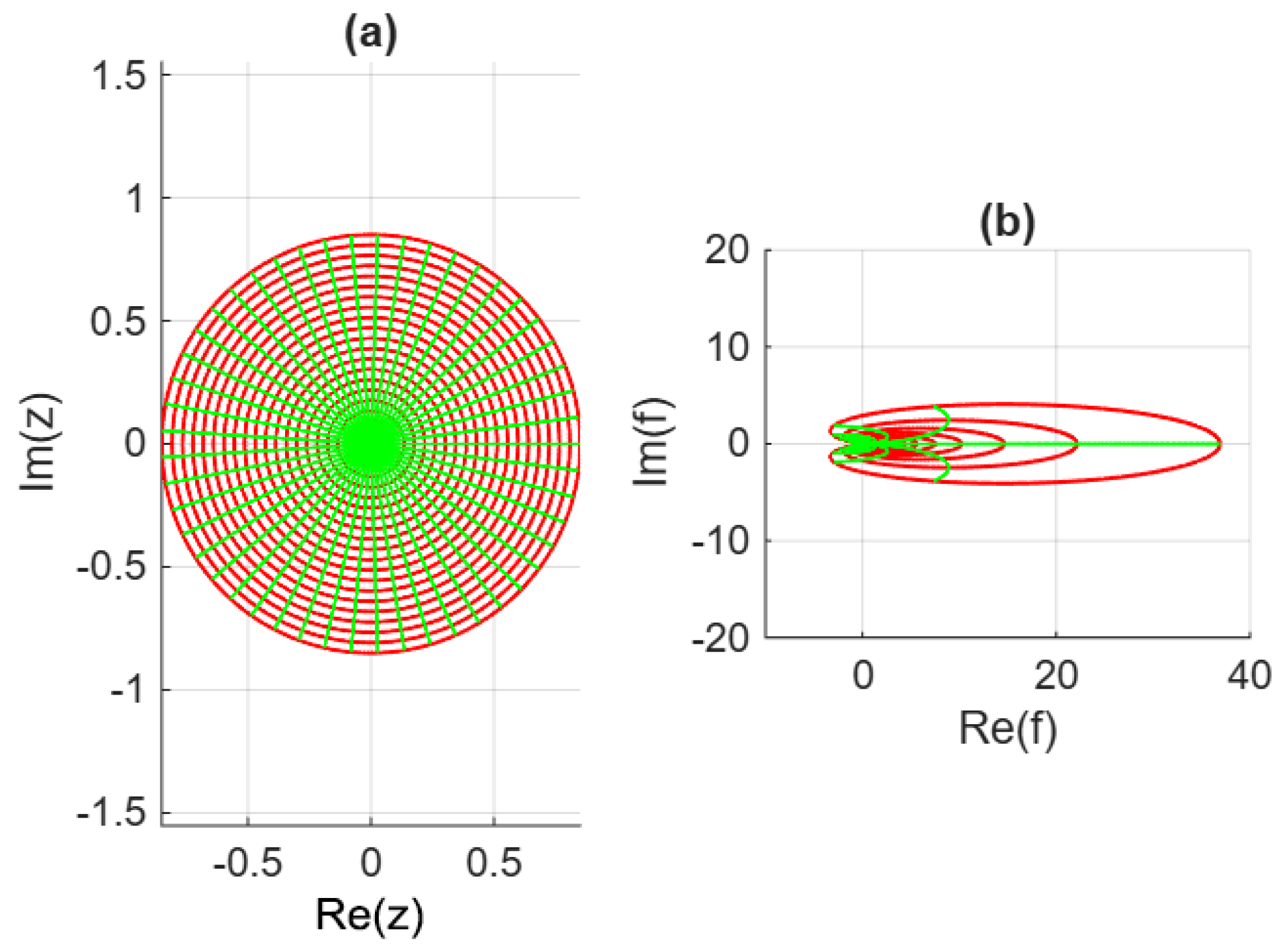
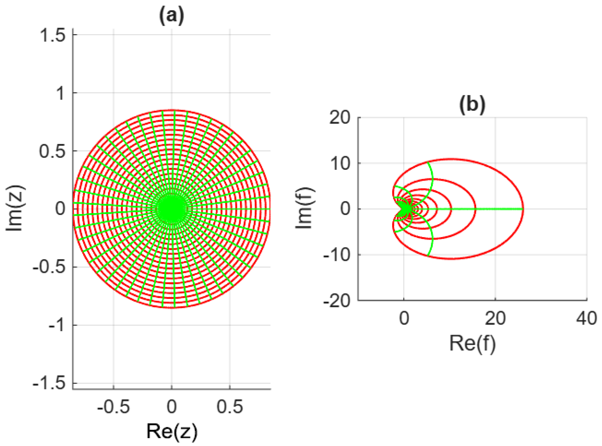
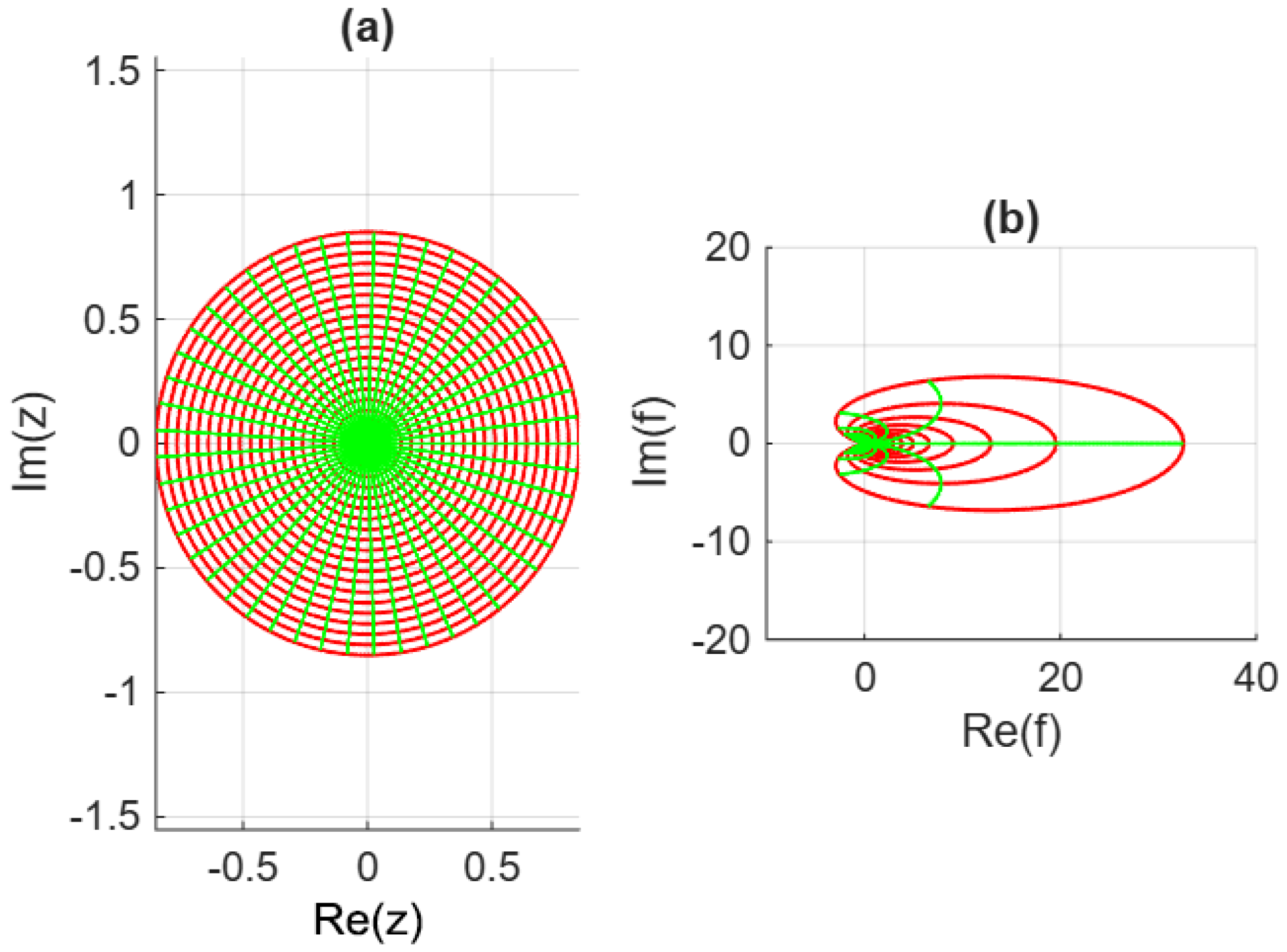
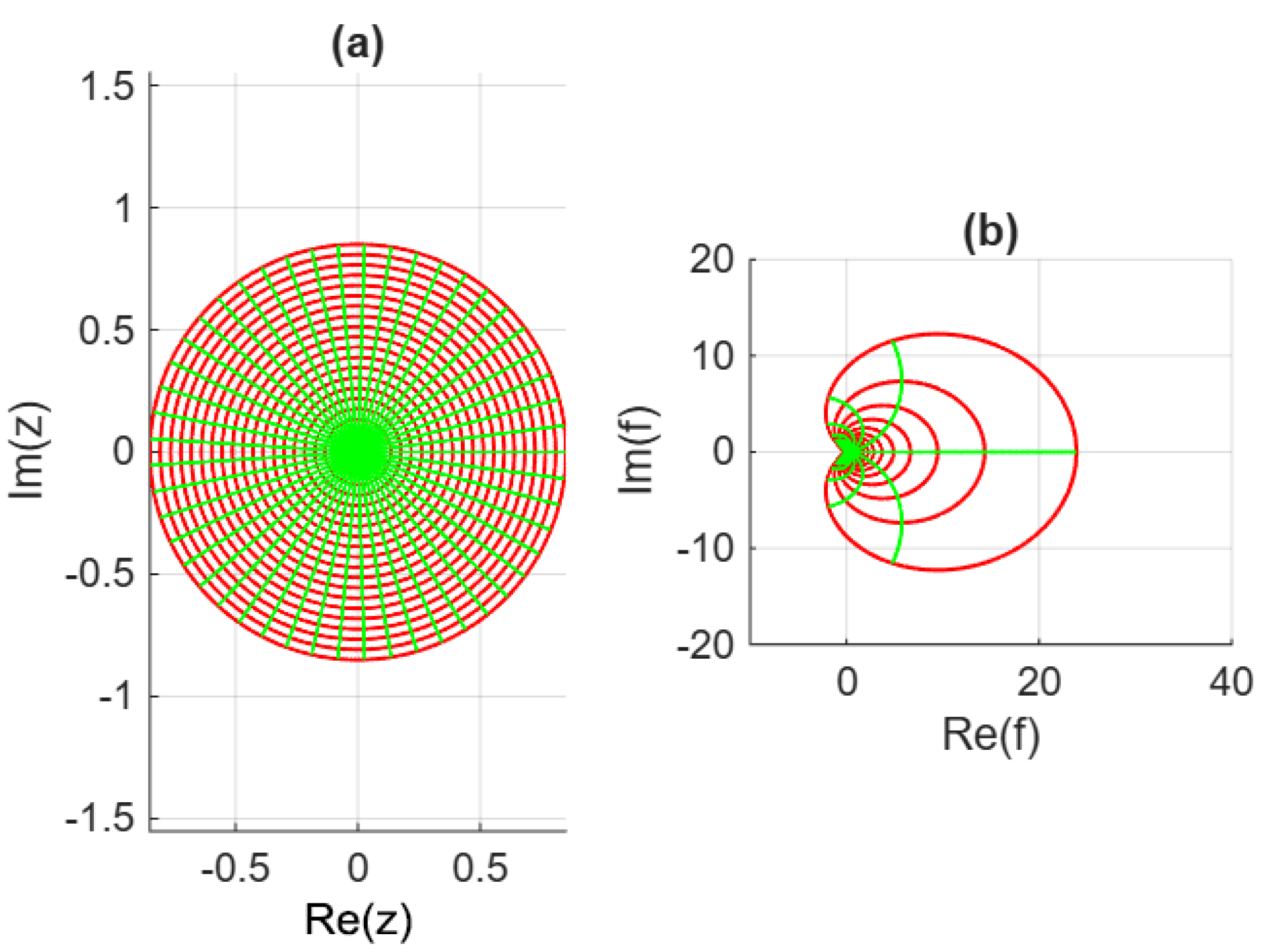
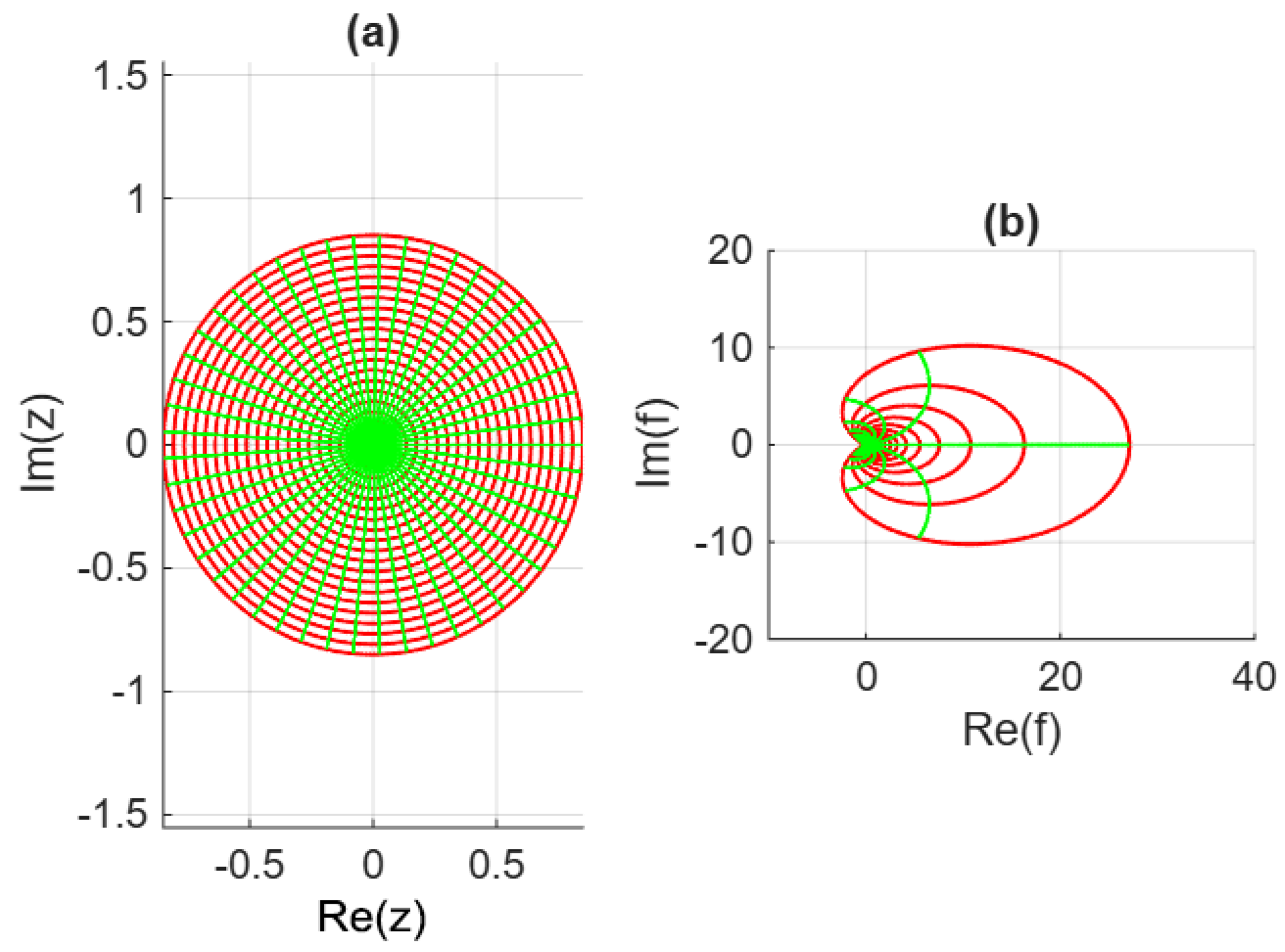
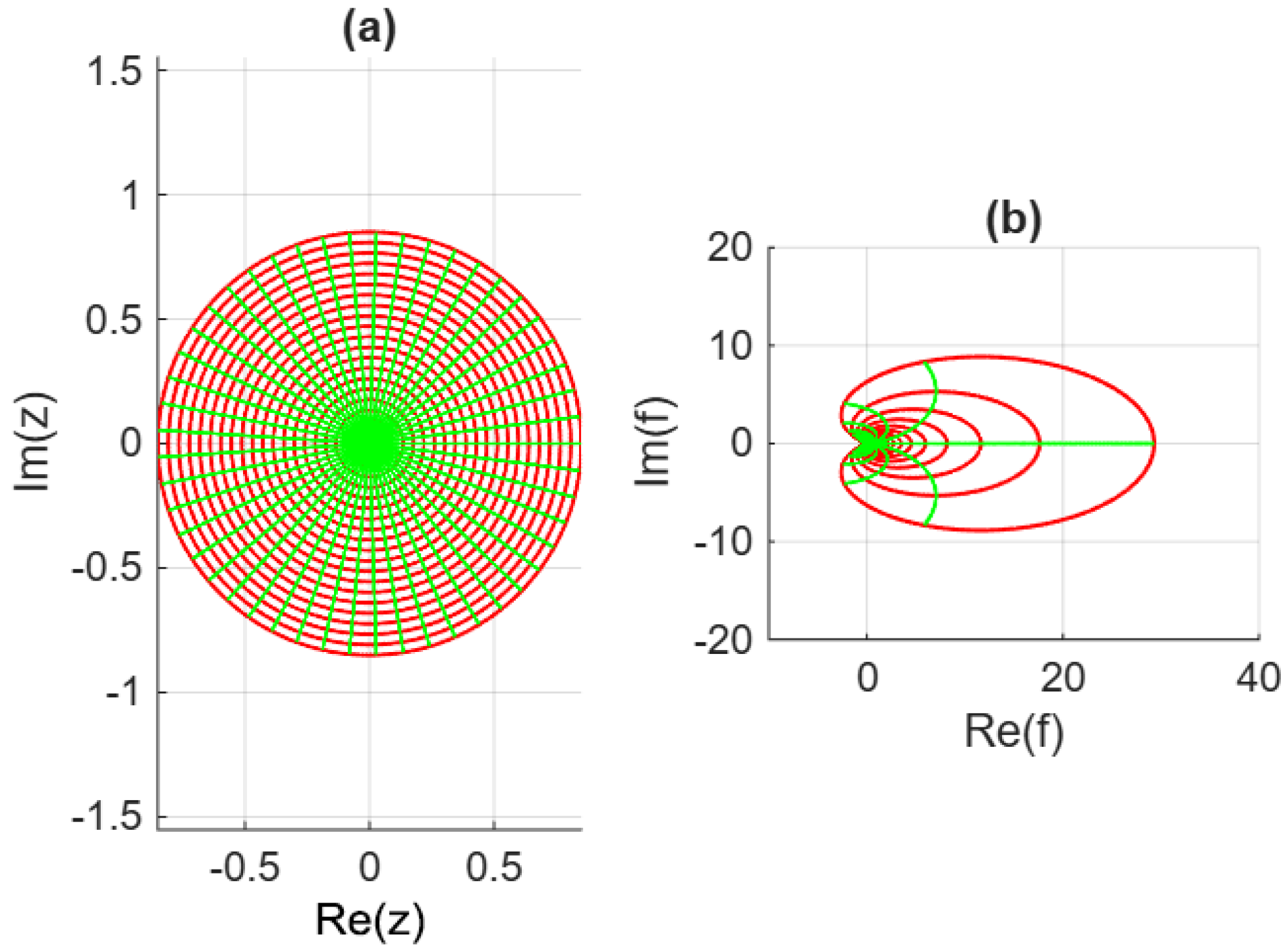
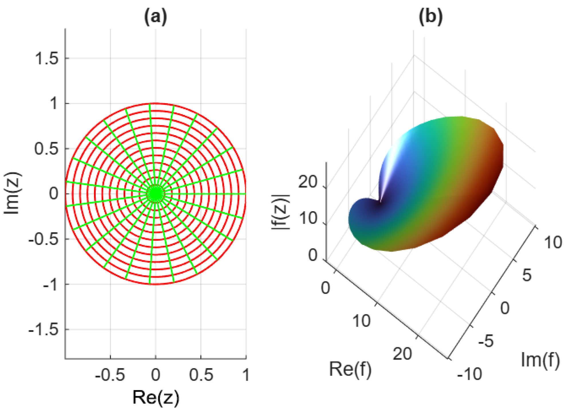
In this section we illustrate the geometric behavior of harmonic mappings belonging to the class $M(\nu ,\tau ,q)$ through several graphical examples. To better understand the geometric behavior of the harmonic mappings in the class $M(\nu ,\tau ,q)$, we present several graphical illustrations of the images of the unit disk under the extremal mappings associated with the class. In each figure, panel (a) shows the unit disk equipped with a polar grid (consisting of concentric circles and radial lines), while panel (b) shows the image of this grid under the harmonic mapping $\phi =l+m$. These plots provide a visual interpretation of how the parameters $\nu$, $\tau$, and q influence the deformation of the unit disk.

Figure 1 illustrates the mapping for the parameters $q=1$, $\nu =0.7$ and $\tau =0.2$. The transformation produces a highly stretched domain in the positive real direction while maintaining smooth curved boundaries. This behavior reflects the influence of the dilatation parameter $\nu$ on the deformation of the analytic part $l\left(\vartheta \right)$.

Figure 2 shows the case $q=1$, $\nu =0.2$ and $\tau =0.2$. Compared to Figure 1, the deformation is less pronounced due to the smaller value of $\nu$. The grid curves remain smoother and the image domain appears more symmetric, illustrating the moderating effect of the dilatation parameter on the harmonic mapping.

Figure 3 corresponds to $q=1$, $\nu =0.5$ and $\tau =0.5$. Increasing the parameter $\tau$ changes the convexity condition of the analytic part $l\left(\vartheta \right)$, which influences the growth of the mapping and produces a different geometric deformation of the unit disk.

Figure 4 and Figure 5 illustrate the case $q=2$ with different values of the parameters $\nu$ and $\tau$. Increasing the valency parameter q introduces additional rotational symmetry in the deformation and leads to more complex geometric patterns in the image domain. The images clearly demonstrate how the higher-order structure of the analytic part affects the global geometry of the mapping.

Figure 6 shows the deformation of the unit disk for $q=2$, $\nu =0.7$ and $\tau =0.2$. The grid transformation highlights the influence of the parameters on the stretching and bending of the domain, confirming the theoretical results established in the preceding sections.

Finally, Figure 7 presents the case $q=2$, $\nu =0.5$ and $\tau =0.5$, where the image of the unit disk is visualized both in the complex plane and in a three-dimensional representation. In the 3D plot, the surface

$$(\Re \phi (\vartheta ),\Im \phi (\vartheta ),|\phi \left(\vartheta \right)\left|\right),\vartheta \in D,$$

illustrates how the magnitude of the mapping varies across the unit disk. The resulting surface provides a clear geometric interpretation of the growth behavior of the harmonic mapping.

These graphical representations demonstrate that harmonic mappings in the class $M(\nu ,\tau ,q)$ transform the unit disk in the domains with smooth boundaries and controlled geometric distortion. The figures also highlight how the parameters $\nu$, $\tau$, and q influence the shape and size of the resulting image domains.

4. Conclusions and Future Directions

In this paper, we introduced a new subclass ($M(\nu ,\tau ,q)$) of q-valent harmonic mappings in the open unit disk related with close-to-convex functions. We first determined that the class $M(\nu ,\tau ,q)$ is non-empty and discussed its relationship with several early known subclasses of harmonic mappings. By employing methods from geometric function theory, we illustrated the close-to-convexity of functions in this class and investigated coefficient estimates for both the analytic and co-analytic parts. Auxiliary lemmas obtained for the analytic part enabled us to establish distortion estimates and prove a growth and distortion theorem. Furthermore, a covering theorem describing the image of the unit disk under functions of this class was obtained.

We also derived sharp bounds for the Fekete–Szegö-type functionals $|a_{q+2}-\lambda a_{q+1}^2|$ and $|b_{q+2}-\lambda b_{q+1}^2|$. In addition, graphical and three-dimensional visualizations provided an analysis of the geometric deformation of the unit disk under the mappings in this class. The results presented in this paper contribute to the geometric theory of multivalent harmonic mappings and extend several known results for harmonic close-to-convex functions.

Future investigations may focus on further geometric and analytic properties of the class $M(\nu ,\tau ,q)$. In particular, it would be interesting to study higher-order coefficient problems, Hankel determinants, convolution properties, and radius problems for this class. Moreover, possible extensions using fractional operators, q-calculus, or other differential operators may lead to new subclasses of harmonic mappings with richer geometric structures.

References

1. Clunie, J.; Sheil-Small, T. Harmonic univalent functions. Ann. Acad. Sci. Fenn. Ser. A. I. Math. 1984, 9, 3–25. [Google Scholar] [CrossRef] [Scilit]
2. Duren, P. Harmonic Mappings in the Plane; Cambridge Tracts in Mathematics; Cambridge University Press: Cambridge, UK, 2004; Volume 156. [Google Scholar]
3. Fekete, M.; Szegö, G. Eine Bemerkung über ungerade schlichte Funktionen. J. Lond. Math. Soc. 1933, 8, 85–89. [Google Scholar] [CrossRef] [Scilit]
4. Abdel-Gawad, D.; Thomas, K. The Fekete–Szegö problem for strong close-to-convex functions. Proc. Am. Math. Soc. 1992, 114, 345–349. [Google Scholar]
5. Koepf, W. On the Fekete–Szegö problem for close-to-convex functions. Proc. Am. Math. Soc. 1987, 101, 89–95. [Google Scholar]
6. Koepf, W. On the Fekete–Szegö problem for close-to-convex functions II. Arch. Math. 1987, 49, 420–433. [Google Scholar] [CrossRef] [Scilit]
7. Mocanu, P.T. Injectivity conditions in the complex plane. Complex Anal. Oper. Theory 2011, 5, 759–766. [Google Scholar] [CrossRef] [Scilit]
8. Bshouty, D.; Lyzzaik, A. Close-to-convexity criteria for planar harmonic mappings. Complex Anal. Oper. Theory 2011, 5, 767–774. [Google Scholar] [CrossRef] [Scilit]
9. Bharanedhar, S.V.; Ponnusamy, S. Coefficient conditions for harmonic univalent mappings and hypergeometric mappings. Rocky Mt. J. Math. 2014, 44, 753–777. [Google Scholar] [CrossRef] [Scilit]
10. Chen, J.; Rasila, A.; Wang, X. Coefficient estimates and radii problems for certain classes of polyharmonic mappings. Complex Var. Elliptic Equ. 2015, 60, 354–371. [Google Scholar] [CrossRef] [Scilit]
11. Mocanu, P.T. Sufficient conditions of univalence for complex functions in the class C. Rev. Anal. Numér. Théor. Approx. 1981, 10, 75–79. [Google Scholar]
12. Nagpal, S.; Ravichandran, V. Starlikeness, convexity and close-to-convexity of harmonic mappings. In Current Topics in Pure and Computational Complex Analysis; Trends in Mathematics; Birkhäuser/Springer: New Delhi, India, 2014; pp. 201–214. [Google Scholar]
13. Hayami, T. Coefficient conditions for harmonic close-to-convex functions. Abstr. Appl. Anal. 2012, 2012, 413965. [Google Scholar] [CrossRef] [Scilit]
14. Arif, M.; Srivastava, H.M.; Raza, M. Convolution properties of meromorphically harmonic functions defined by a generalized convolution q-derivative operator. AIMS Math. 2021, 6, 5869–5885. [Google Scholar] [CrossRef] [Scilit]
15. Arif, M.; Haq, M.U.; Liu, J.L. A subfamily of univalent functions associated with q-analogue of Noor integral operator. J. Funct. Spaces 2018, 2018, 3818915. [Google Scholar] [CrossRef] [Scilit]
16. Arif, M.; Barkub, O.; Srivastava, H.M.; Abdullah, S.; Khan, S.A. Some Janowski type harmonic q-starlike functions associated with symmetrical points. Mathematics 2020, 8, 629. [Google Scholar] [CrossRef] [Scilit]
17. Li, L.; Ponnusamy, S. Injectivity of sections of univalent harmonic mappings. Nonlinear Anal. Theory Methods Appl. 2013, 89, 276–283. [Google Scholar] [CrossRef] [Scilit]
18. Li, L.; Ponnusamy, S. Sections of stable harmonic convex functions. Nonlinear Anal. Theory Methods Appl. 2015, 123–124, 178–190. [Google Scholar] [CrossRef] [Scilit]
19. Wang, X.Y.; Wang, Z.G.; Fan, J.H.; Zhang, Y.; Liu, J.G. Some properties of certain close-to-convex harmonic mappings. Anal. Math. Phys. 2022, 12, 28. [Google Scholar] [CrossRef] [Scilit]
20. Hadi, S.H.; Darus, M.; Lupaş, A.A. A class of Janowski-type (p,q)-convex harmonic functions involving a generalized q-Mittag–Leffler function. Axioms 2023, 12, 190. [Google Scholar] [CrossRef] [Scilit]
21. Sayyari, Y.; Dehghanian, M. A new class of convex functions and applications in entropy and analysis. Chaos Solitons Fractals 2024, 181, 114677. [Google Scholar] [CrossRef] [Scilit]
22. Cotîrlă, L.-I.; Totoi, E.-A. Similar classes of convex and close-to-convex meromorphic functions obtained through integral operators. Symmetry 2024, 16, 1604. [Google Scholar] [CrossRef] [Scilit]
23. Aoen; Li, S.; Tula; Li, S.; Gao, H. New subclass of generalized close-to-convex function related with quasi-subordination. AIMS Math. 2025, 10, 12149–12167. [Google Scholar] [CrossRef] [Scilit]
24. Sakar, F.M.; Omendra, M.; Oros, G.I.; Frasin, B.A. On certain bounds of harmonic univalent functions. Axioms 2025, 14, 393. [Google Scholar] [CrossRef] [Scilit]
25. Sun, Y.; Jiang, Y.-P.; Rasila, A. On a subclass of close-to-convex harmonic mappings. Complex Var. Elliptic Equ. 2016, 61, 1627–1643. [Google Scholar] [CrossRef] [Scilit]
26. Carathéodory, C. Über den Variabilitätsbereich der Fourier’schen Konstanten von positiven harmonischen Funktionen. Rend. Circ. Palermo 1911, 32, 193–217. [Google Scholar] [CrossRef] [Scilit]
27. Pommerenke, C. Univalent Functions; Vandenhoeck & Ruprecht: Göttingen, Germany, 1975. [Google Scholar]
28. Goodman, A.W. Univalent Functions; Mariner: Tampa, FL, USA, 1983. [Google Scholar]
29. Suffridge, T.J. Some special classes of conformal mappings. In Handbook of Complex Analysis: Geometric Function Theory; Kühnau, R., Ed.; Elsevier: Amsterdam, The Netherlands, 2005; Volume 2, pp. 309–338. [Google Scholar]
Figure 1. (a) The unit disk with circular and radial grids. (b) Image of the unit disk under the harmonic mapping f for p = 1 , α = 0.7 , and β = 0.2 .
Mathematics 14 02062 g001
Figure 2. (a) Image of the unit disk. (b) Image of the unit disk under the harmonic mapping f for p = 1 , α = 0.2 , and β = 0.2 .
Mathematics 14 02062 g002
Figure 3. (a) Image of unit disk. (b) Image of the unit disk under the harmonic mapping f for p = 1 , α = 0.5 , and β = 0.5 .
Mathematics 14 02062 g003
Figure 4. (a) Image of unit disk. (b) Image of the unit disk under the harmonic mapping f for p = 2 , α = 0.2 , and β = 0.2 .
Mathematics 14 02062 g004
Figure 5. (a) Image of unit disk. (b) Three-dimensional visualization of the image of the unit disk under the mapping f for p = 2 , α = 0.5 , and β = 0.5 .
Mathematics 14 02062 g005
Figure 6. (a) Image of unit disk. (b) Image of the unit disk under the harmonic mapping f for p = 2 , α = 0.7 , and β = 0.2 .
Mathematics 14 02062 g006
Figure 7. (a) Image of unit disk. (b) Image of the unit disk under the harmonic mapping f for p = 2 , α = 0.5 , and β = 0.5 .
Mathematics 14 02062 g007
Disclaimer/Publisher’s Note: The statements, opinions and data contained in all publications are solely those of the individual author(s) and contributor(s) and not of MDPI and/or the editor(s). MDPI and/or the editor(s) disclaim responsibility for any injury to people or property resulting from any ideas, methods, instructions or products referred to in the content.