Structural Characterization and Inference for an Odds-Scale Lomax Model with Applications to Unit-Interval Data

Abstract

This paper develops a structural, inferential, and computational study of a Lomax-based model on a unit interval obtained through the odds transformation $Z=Y/(1+Y)$ of a baseline Lomax random variable. Rather than proposing a genuinely new unit distribution, the paper clarifies the model’s exact position in the literature by showing that it is equivalent, up to complementation and reparametrization, to a previously reported unit-Lomax-type construction. The contribution is therefore focused on its odds-scale interpretation, analytical tractability, and reliable inference. We derive the main distributional functions, endpoint behavior, hazard shapes, quantiles, moments, and odds-scale representations. We also show that likelihood inference reduces to classical Lomax inference on the odds-transformed sample, which explains the severe maximum likelihood estimator instability observed in small-sample and heavy-tailed regimes. To address this issue, we complement maximum likelihood estimation with maximum product of spacings estimation. Monte Carlo experiments and real-data applications illustrate that the maximum likelihood estimator may be reliable for moderate tail behavior and sufficiently large samples, whereas the MPS estimator provides a more stable alternative in challenging finite-sample settings.

1. Introduction

In many applied fields, including engineering, environmental sciences, economics, and biomedicine, the variable of interest is a rate, fraction, or proportion bounded in the unit interval $(0,1)$. Typical examples include conversion rates in online marketing, defect fractions in quality control, success proportions in clinical trials, and coverage or usage ratios in environmental and ecological studies. For this type of data, the beta distribution has become a standard reference model because of its flexibility in terms of skewness and kurtosis, as well as the availability of well-established inferential and regression methodologies, such as beta regression for modeling rates and proportions [1,2].

The Kumaraswamy distribution is an important alternative to the beta distribution for modeling bounded random variables. It was originally introduced in the context of double-bounded random processes [3]. Its cumulative distribution and quantile functions are available in closed form, which facilitates random variate generation as well as estimation by maximum likelihood and moments. In the last decade, both beta and Kumaraswamy distributions have often been used as baseline models to construct more general families via different generator schemes, leading to a broad class of unit distributions with one or more additional shape parameters.

In parallel, the literature on general methods for generating new families of continuous distributions has grown considerably. Influential contributions include the Marshall–Olkin approach, which adds a parameter at the level of the survival function [4], the T-X method based on transforming a baseline variable through a generator function [5], and the so-called “odds” or “odds-x” families, which rely on transformations of the form $F\left(x\right)/(1-F(x\left)\right)$ [6] and related odds-based constructions [7]. Recent reviews systematize these approaches in terms of transformation-based generators and compounding mechanisms, highlighting the central role of beta-generated and T-X-type constructions in building flexible univariate families [8].

Despite these advances, in the specific context of unit distributions, many of the available models are based on baseline distributions with relatively light tails, such as the normal, gamma, or Weibull distributions, or on direct extensions of the beta and Kumaraswamy laws. This may limit their ability to capture heavy-tailed behavior or complex risk structures when the data are naturally linked, through a monotonic transformation, to heavy-tailed positive variables. In many applications, a proportion $Z\in (0,1)$ can be interpreted as a monotonic transform of a positive variable Y, for example, when Y represents failure times, traffic intensities, or claim sizes, and Z is a ratio-type quantity built from these latent variables.

The Lomax distribution (also known as Pareto type II) is a classical model for non-negative data with heavy tails, widely used in reliability, insurance, traffic analysis, and economics [9]. Its cumulative distribution function on $[0,\infty )$ exhibits a power-law tail and a decreasing hazard rate, which makes it suitable for describing survival phenomena with “wear-out” or cleansing effects. Building on this baseline, an extensive family of Lomax-based extensions has been proposed in the literature, such as the extended Lomax distribution [10] and the Weibull–Lomax distribution [11], among others. These models display a rich variety of density and hazard shapes, including increasing, decreasing, unimodal, and bathtub-shaped hazards.

The explicit incorporation of this kind of heavy-tail behavior into models with support on $(0,1)$ has received comparatively less attention. From a conceptual perspective, it is natural to consider unit distributions obtained by applying the inverse logit or other monotonic mappings from $(0,\infty )$ to $(0,1)$ for Lomax-distributed variables. This strategy allows the model to inherit part of the heavy-tail structure of the baseline Lomax distribution on the odds scale while producing a distribution that is directly interpretable in terms of rates or proportions.

Related unit-interval models based on Lomax-type baselines have recently appeared in the literature, including exponentiated and regression-oriented extensions on $(0,1)$ [12] and the unit ratio-extended Weibull family of [13], of which the present model is a particular case. In addition, several recent contributions have proposed transformed or unit-interval models for proportional data, including unit Burr-XII and quantile-regression formulations [14], alternative unit-Lindley-type models [15], unit exponential and related transformed models [16], new bounded and power-unit constructions [17,18], and recent Chen- and Weibull-type unit models [19,20,21]. This active literature makes it important to distinguish between algebraic reformulations, genuinely different generators, and equivalent constructions obtained through monotone maps.

Motivated by this point, we study a bounded model with a cumulative distribution function

$$F_Z(z;\alpha ,\beta )=1-{\left(1+{\displaystyle \frac{z}{\beta (1-z)}}\right)}^{-\alpha },0<z<1,\alpha >0,\beta >0,$$

which arises from the odds transformation $Z=Y/(1+Y)$ with $Y\sim \mathrm{Lomax}(\alpha ,\beta )$. This representation is not merely a reparametrization device; it provides a transparent structural link between heavy-tail behavior on the positive half-line and interpretable shape behavior on the unit interval while preserving analytic tractability.

The contribution of this paper is primarily structural, inferential, and computational, and it should be interpreted as a complement to previously reported unit-Lomax-type constructions rather than as the introduction of a genuinely new distributional family. More precisely, the contribution is threefold. First, we establish explicitly the equivalence between the present odds-scale formulation and a previously studied unit-Lomax-type construction, up to complementation and reparametrization, thereby clarifying issues of nomenclature and avoiding an overstatement of novelty. Second, we emphasize the representation $Z=Y/(1+Y)$, $Y\sim \mathrm{Lomax}(\alpha ,\beta )$, which gives the model a direct odds-scale interpretation in terms of a latent positive heavy-tailed variable. Third, we study the inferential consequences of this representation. In particular, we show that the likelihood for the unit-interval model is equivalent to the classical Lomax likelihood applied to the odds-transformed observations $Y_i=Z_i/(1-Z_i)$. This observation explains why maximum likelihood estimation may become unstable in small samples or under heavy-tailed parameter configurations. To address this issue, the revised inferential framework includes maximum product of spacings estimation as a more stable alternative in challenging finite-sample settings.

Accordingly, the paper should be viewed as a detailed structural, inferential, and computational reassessment of an odds-scale representation of a Lomax-based unit model. This perspective is especially relevant when bounded observations are naturally interpreted through latent positive mechanisms with heavy-tailed behavior on the odds scale.

The remainder of the paper is organized as follows. Section 2 presents the model, its equivalence with previous unit-Lomax-type constructions, and its main structural properties. Section 3 develops likelihood-based inference, diagnoses finite-sample maximum likelihood estimator instability, and introduces maximum product of spacings estimation. Section 4 describes random variate generation. Section 5 reports the Monte Carlo study comparing the maximum likelihood estimator and MPS. Section 6 presents the data applications and model comparisons. Section 7 concludes the paper.

2. Structural Properties and Tractability

In this section, we record the structural facts that are used later in the inferential and computational analysis. Since the model is generated by the monotone transformation $Z=Y/(1+Y)$, the cdf, pdf, survival, hazard, and quantile functions follow directly from the Lomax baseline and are therefore stated in compact form. Greater attention is given to endpoint behavior, hazard shapes, and modality since these properties are more informative for applications and for the finite-sample inference discussed in Section 3.

2.1. Definition, Density and Hazard Functions

Definition 1.

Let Y be a Lomax (Pareto type II) random variable with shape parameter $\alpha >0$ and scale parameter $\beta >0$, that is,

$$F_Y(y;\alpha ,\beta )=1-{\left(1+{\displaystyle \frac{y}{\beta }}\right)}^{-\alpha },y>0,\alpha >0,\beta >0,$$

(1)

with the corresponding probability density function

$$f_Y(y;\alpha ,\beta )={\displaystyle \frac{\alpha }{\beta }}{\left(1+{\displaystyle \frac{y}{\beta }}\right)}^{-(\alpha +1)},y>0.$$

(2)

Consider the monotonic transformation

$$Z=T\left(Y\right)={\displaystyle \frac{Y}{1+Y}}\in (0,1),$$

(3)

whose inverse is

$$T^{-1}\left(z\right)={\displaystyle \frac{z}{1-z}},0<z<1,$$

with Jacobian

$${\displaystyle \frac{d}{dz}}{T}^{-1}\left(z\right)={\displaystyle \frac{1}{{(1-z)}^2}},0<z<1.$$

(4)

A random variable Z is said to follow an odds-Lomax distribution with parameters $(\alpha ,\beta )$, denoted by $Z\sim OL(\alpha ,\beta )$, if it admits the stochastic representation (3) with $Y\sim \mathrm{Lomax}(\alpha ,\beta )$ as in (1). By construction, Z takes values in the open unit interval $(0,1)$.

Proposition 1.

Let U be a random variable on $(0,1)$ with a distribution function

$$T\left(u\right)={\left(1+b\left(u^{-1}-1\right)\right)}^{-a},0<u<1,$$

for some $a>0$ and $b>0$. Define $Z=1-U$. Then Z has the cdf

$$F_Z\left(z\right)=1-{\left(1+{\displaystyle \frac{z}{\beta (1-z)}}\right)}^{-\alpha },0<z<1,$$

with $\alpha =a$ and $\beta =1/b$. Hence, the odds-Lomax formulation is equivalent, up to simple complementary transformation and reparametrization, to the unit-Lomax-type construction considered in [22].

Proof. 

For $0<z<1$,

$$F_Z\left(z\right)=\mathbb{P}(Z\le z)=\mathbb{P}(1-U\le z)=\mathbb{P}(U\ge 1-z)=1-T(1-z).$$

Substituting into T gives

$$F_Z\left(z\right)=1-{\left(1+b\left({(1-z)}^{-1}-1\right)\right)}^{-a}=1-{\left(1+b{\displaystyle \frac{z}{1-z}}\right)}^{-a}.$$

Setting $\alpha =a$ and $\beta =1/b$ yields the stated form.    □

Remark 1.

Proposition 1 shows that the present formulation is best understood as an odds-scale representation of a Lomax-based unit-interval model. The terminology odds-Lomax is adopted here to emphasize the transformation $Z=Y/(1+Y)$ and to avoid confusion with other non-equivalent families that have also been described in the literature under the label “unit-Lomax”.

Remark 2.

In addition, the present model is a particular case of the unit ratio-extended Weibull family introduced by [13], with the present formulation corresponding to the Lomax-based odds-scale case within that family. The present paper should therefore be understood not as introducing a new distributional family, but as providing a detailed structural, inferential, and computational study of this specific odds-scale Lomax formulation, with particular emphasis on the MLE instability mechanism and the role of MPS as a robust alternative.

Proposition 2.

If $Z\sim OL(\alpha ,\beta )$, then for $0<z<1$,

$$\begin{array}{c}{F}_Z(z;\alpha ,\beta )=1-{\left(1+{\displaystyle \frac{z}{\beta (1-z)}}\right)}^{-\alpha },\end{array}$$

(5)

$$\begin{array}{c}{f}_Z(z;\alpha ,\beta )={\displaystyle \frac{\alpha {\beta }^{\alpha }{(1-z)}^{\alpha -1}}{{(\beta +(1-\beta )z)}^{\alpha +1}}},\end{array}$$

(6)

$$\begin{array}{c}{S}_Z(z;\alpha ,\beta )={\left({\displaystyle \frac{\beta (1-z)}{\beta +(1-\beta )z}}\right)}^{\alpha },\end{array}$$

(7)

$$\begin{array}{c}{h}_Z(z;\alpha ,\beta )={\displaystyle \frac{\alpha }{(\beta +(1-\beta \left)z\right)(1-z)}}.\end{array}$$

(8)

These expressions follow directly from the monotone transformation $z=y/(1+y)$, its inverse $y=z/(1-z)$, and the change-of-variables formula.

The odds-Lomax model has parameter-independent support $(0,1)$, and for $\alpha >0$ and $\beta >0$, its density (6) is continuously differentiable in z on $(0,1)$. These properties support the standard maximum likelihood regularity conditions used in Section 3.

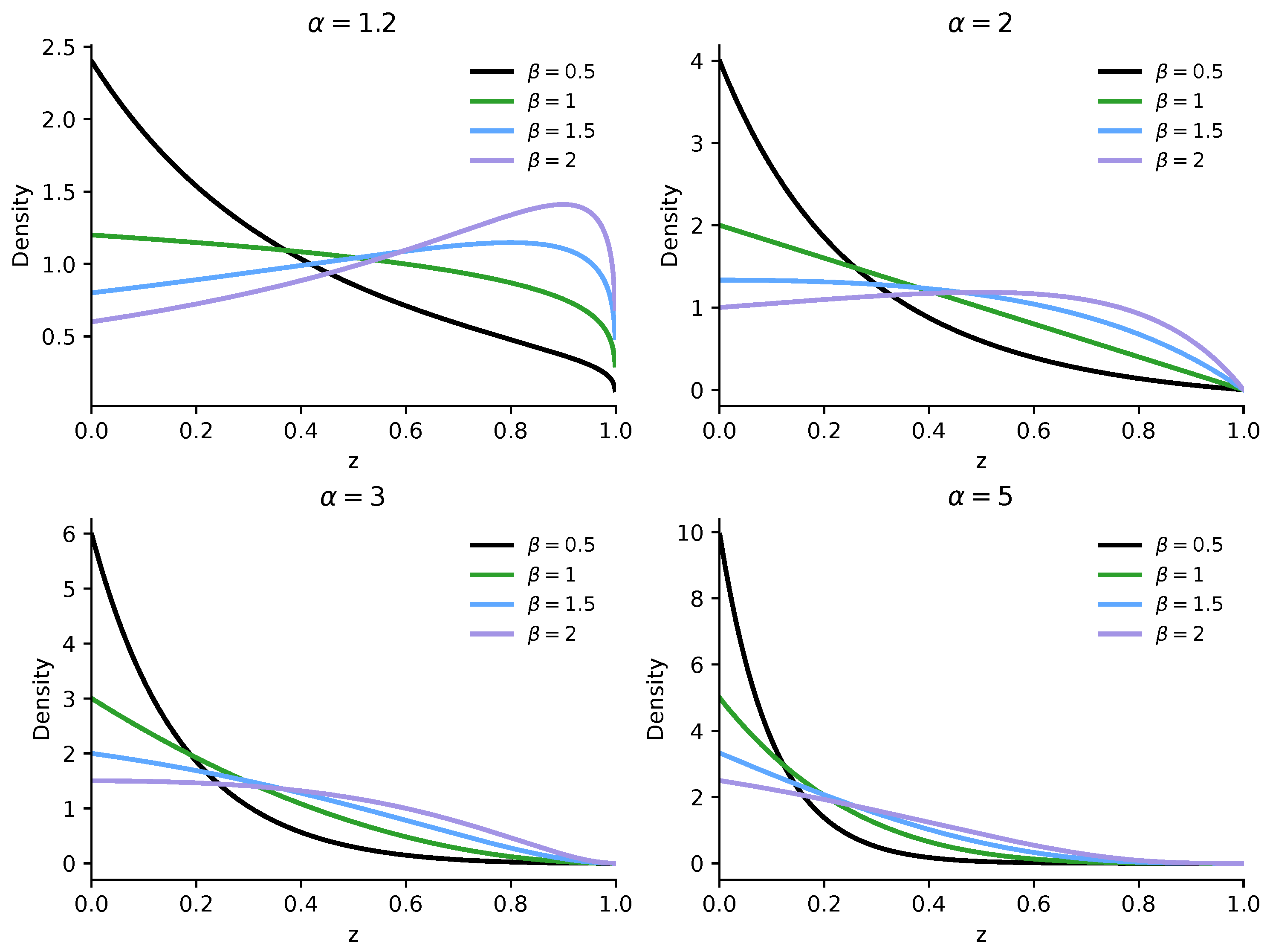
Figure 1 displays representative shapes of the odds-Lomax density for selected combinations of $(\alpha ,\beta )$, highlighting the variety of forms that the model can exhibit on the unit interval, including decreasing, increasing, unimodal, and U-shaped patterns.

2.2. Limiting Behavior and Shape Properties

The behavior of the density and hazard functions near the boundaries $z\to 0$ and $z\to 1$, as well as the main shapes that can arise for the hazard function, is examined next.

Proposition 3.

Let $Z\sim OL(\alpha ,\beta )$. Then

$$\begin{array}{c}\underset{z\to 0^{+}}{\lim }{f}_Z(z;\alpha ,\beta )={\displaystyle \frac{\alpha }{\beta }},\end{array}$$

(9)

$$\begin{array}{c}\underset{z\to 1^{-}}{\lim }{f}_Z(z;\alpha ,\beta ){(1-z)}^{1-\alpha }=\alpha {\beta }^{\alpha },\end{array}$$

(10)

$$\begin{array}{c}\underset{z\to 1^{-}}{\lim }{\displaystyle \frac{S_Z(z;\alpha ,\beta )}{{(1-z)}^{\alpha }}}={\beta }^{\alpha }.\end{array}$$

(11)

In particular,

$$\underset{z\to 1^{-}}{\lim }{f}_Z(z;\alpha ,\beta )=\left\{\begin{array}{cc}0,\hfill & \alpha >1,\hfill \\ \beta ,\hfill & \alpha =1,\hfill \\ +\infty ,\hfill & 0<\alpha <1,\hfill \end{array}\right.$$

whereas the survival function decays to zero at the polynomial rate $S_Z(z;\alpha ,\beta )\sim {\beta }^{\alpha }{(1-z)}^{\alpha }$ as $z\to 1^{-}$.

These limits follow directly from the explicit forms of the density and survival functions in (6) and (7) by evaluating the leading terms as $z\to 0^{+}$ and $z\to 1^{-}$.

Proposition 3 shows that the odds-Lomax density is always finite and strictly positive at $z=0$, while its behavior near $z=1$ depends on the shape parameter $\alpha$. For $\alpha >1$, the density vanishes at 1, whereas for $0<\alpha <1$, it diverges as ${(1-z)}^{\alpha -1}$. This allows the model to accommodate both relatively light right tails on the probability scale (for large $\alpha$) and highly concentrated mass near $z=1$ (for small $\alpha$), which is particularly useful when modeling proportions close to one.

The tail representation (11) also highlights the role of $\alpha$ as a tail index on the odds scale: the survival function of Z inherits the polynomial decay of the Lomax baseline under the transformation $z\mapsto z/(1-z)$, with $\alpha$ controlling the order of decay and $\beta$ acting as a scale parameter.

Proposition 4.

For $Z\sim OL(\alpha ,\beta )$, the hazard function (8) satisfies

$$\begin{array}{c}\underset{z\to 0^{+}}{\lim }{h}_Z(z;\alpha ,\beta )={\displaystyle \frac{\alpha }{\beta }},\end{array}$$

(12)

$$\begin{array}{c}\underset{z\to 1^{-}}{\lim }{h}_Z(z;\alpha ,\beta )(1-z)=\alpha ,\end{array}$$

(13)

and its derivative is given by

$$h_Z^{\prime }(z;\alpha ,\beta )={\displaystyle \frac{\alpha \left(2\beta -1+2(1-\beta )z\right)}{{\left(\beta +(1-\beta )z\right)}^2{(1-z)}^2}},0<z<1.$$

(14)

Consequently:

(i) 

If $\beta \ge 1/2$, then $h_Z^{\prime }(z;\alpha ,\beta )>0$ for all $z\in (0,1)$, so the hazard is strictly increasing.

(ii) 

If $0<\beta <1/2$, then there exists a unique

$$z_h^{*}={\displaystyle \frac{1-2\beta }{2(1-\beta )}}\in (0,1)$$

such that $h_Z^{\prime }(z;\alpha ,\beta )<0$ for $0<z<z_h^{*}$ and $h_Z^{\prime }(z;\alpha ,\beta )>0$ for $z_h^{*}<z<1$, so the hazard is strictly decreasing on $(0,z_h^{*})$ and strictly increasing on $(z_h^{*},1)$, displaying a bathtub-shaped hazard.

The result follows by differentiating the closed-form hazard function in (8) and analyzing the sign of the resulting affine numerator.

Remark 3.

Proposition 4 shows that the odds-Lomax distribution can produce two qualitatively distinct hazard shapes on $(0,1)$. When $\beta \ge 1/2$, the hazard function is strictly increasing, which may be appropriate for processes where the instantaneous risk grows as the proportion approaches one. In contrast, for $0<\beta <1/2$, the hazard is bathtub-shaped, reflecting an initial decrease in risk followed by an increasing phase, a pattern often encountered in reliability and survival applications. Interestingly, these shapes are controlled entirely by the scale parameter β, whereas the shape parameter α acts as a vertical scaling factor for the hazard function.

2.3. Quantiles and Modes

In this subsection, the quantile function of the odds-Lomax distribution is derived, and the location of its mode (or modes) is characterized as a function of the parameters $(\alpha ,\beta )$.

Proposition 5.

Let $Z\sim OL(\alpha ,\beta )$ with cdf given by (5). Then the quantile function $Q:(0,1)\to (0,1)$, defined by $Q\left(u\right)=F_Z^{-1}(u;\alpha ,\beta )$, is

$$Q(u;\alpha ,\beta )={\displaystyle \frac{\beta \left({(1-u)}^{-1/\alpha }-1\right)}{1+\beta \left({(1-u)}^{-1/\alpha }-1\right)}},0<u<1.$$

(15)

In particular, the median m of Z is given by $m=Q(1/2;\alpha ,\beta )$.

Equation (15) follows from the direct inversion of the cdf and is retained because it provides the inversion sampler used in Section 4.

Attention now turns to the mode. Let $f_Z$ denote the density (6) and consider the log-density

$$\ell (z;\alpha ,\beta )=\log \left(\alpha \right)+\alpha \log \left(\beta \right)+(\alpha -1)\log (1-z)-(\alpha +1)\log \left(\beta +(1-\beta )z\right).$$

(16)

Differentiating with respect to z,

$${\ell }^{\prime }(z;\alpha ,\beta )=-{\displaystyle \frac{\alpha -1}{1-z}}-{\displaystyle \frac{(\alpha +1)(1-\beta )}{\beta +(1-\beta )z}},0<z<1.$$

The stationary points of the density are obtained by solving ${\ell }^{\prime }(z;\alpha ,\beta )=0$. The next result characterizes the modality of the odds-Lomax density, including the existence of an interior stationary point and the boundary-mode behavior. Since the support is the open interval $(0,1)$, statements such as “mode at $z=0$” are understood in the limiting sense as $z\to 0^{+}$ (analogously for $z\to 1^{-}$).

Proposition 6.

Let $Z\sim OL(\alpha ,\beta )$ with $\alpha >0$ and $\beta >0$.

(i) 

If $\beta =1$, then $Z\sim \mathrm{Beta}(1,\alpha )$ with density

$$f_Z(z;\alpha ,1)=\alpha {(1-z)}^{\alpha -1},0<z<1.$$

In this case, the density is

(a) 

Strictly decreasing (L-shaped) for $\alpha >1$;

(b) 

Constant (uniform) for $\alpha =1$; and

(c) 

Strictly increasing (J-shaped) for $0<\alpha <1$.

(ii) 

If $\beta \ne 1$, then the log-density (16) admits at most one stationary point in $(0,1)$, given by

$$z_m^{*}(\alpha ,\beta )={\displaystyle \frac{-\alpha +2\beta -1}{2(\beta -1)}}={\displaystyle \frac{\alpha +1-2\beta }{2(1-\beta )}}.$$

(17)

Moreover, the following cases hold:

(a) 

If $\beta >1$ and $1<\alpha <2\beta -1$, then $z_m^{*}\in (0,1)$, and $f_Z$ is unimodal, with a unique interior mode at $z_m^{*}$.

(b) 

If $\beta >1$ and $0<\alpha \le 1$, then $f_Z$ is strictly increasing on $(0,1)$, with ${\sup }_{0<z<1}{f}_Z(z;\alpha ,\beta )={\lim }_{z\to 1^{-}}{f}_Z(z;\alpha ,\beta )$ (unbounded if $0<\alpha <1$ and finite if $\alpha =1$).

(c) 

If $\beta >1$ and $\alpha \ge 2\beta -1$, then $f_Z$ is strictly decreasing on $(0,1)$, with ${\sup }_{0<z<1}{f}_Z(z;\alpha ,\beta )={\lim }_{z\to 0^{+}}{f}_Z(z;\alpha ,\beta )$.

(d) 

If $\beta <1$ and $2\beta -1<\alpha <1$, then $z_m^{*}\in (0,1)$ and $f_Z$ has a unique interior minimum at $z_m^{*}$, decreasing on $(0,z_m^{*})$ and increasing on $(z_m^{*},1)$.

The modality classification follows from differentiating the log-density in (16), solving ${\ell }^{\prime }(z;\alpha ,\beta )=0$, and combining the sign of ${\ell }^{\prime }$ with the endpoint behavior in Proposition 3. The odds-Lomax family can therefore accommodate a wide variety of density shapes on the unit interval, including L- and J-shaped, unimodal, and U-shaped patterns, with the parameters $\alpha$ and $\beta$ exerting distinct control over tail behavior and modality.

2.4. Moments and Entropies

This section derives expressions for the raw moments of the $OL(\alpha ,\beta )$ distribution using its Lomax-based stochastic representation and discusses the existence conditions and some consequences for moment-based measures, such as the mean and variance. Since entropy is not central to the inferential contribution of the paper, a compact Shannon entropy expression is recorded only as an ancillary descriptive quantity.

2.4.1. Raw Moments via the Lomax Representation

Let $Z\sim OL(\alpha ,\beta )$ and recall that

$$Y={\displaystyle \frac{Z}{1-Z}}\sim \mathrm{Lomax}(\alpha ,\beta ),Z={\displaystyle \frac{Y}{1+Y}},$$

with Lomax density

$$f_Y(y;\alpha ,\beta )={\displaystyle \frac{\alpha }{\beta }}{\left(1+{\displaystyle \frac{y}{\beta }}\right)}^{-(\alpha +1)},y>0.$$

For $r>-1$, the rth raw moment of Z can be written as

$${\mu }_r^{\prime }=\mathbb{E}\left(Z^r\right)=\mathbb{E}\left({\left({\displaystyle \frac{Y}{1+Y}}\right)}^r\right)={\displaystyle \frac{\alpha }{\beta }}{\int }_0^{\infty }{\left({\displaystyle \frac{y}{1+y}}\right)}^r{\left(1+{\displaystyle \frac{y}{\beta }}\right)}^{-(\alpha +1)}dy.$$

(18)

Using the odds-scale Lomax representation and the standard Euler-type integral identity, the raw moments admit the following compact expression.

Proposition 7.

Let $Z\sim OL(\alpha ,\beta )$ with $\alpha >0$ and $\beta >0$. Then, for every $r>-1$, the power moment ${\mu }_r^{\prime }=\mathbb{E}\left(Z^r\right)$ exists and is given by

$${\mu }_r^{\prime }=\alpha {\beta }^r{\displaystyle \frac{\Gamma (r+1)\Gamma \left(\alpha \right)}{\Gamma (r+\alpha +1)}}{}_{2}F_1\left(r,r+1;r+\alpha +1;1-\beta \right).$$

(19)

In particular, ${\mu }_0^{\prime }=1$, and all integer raw moments of order $r\ge 0$ exist.

For integer $r\ge 0$, the beta function simplifies to

$$B(r+1,\alpha )={\displaystyle \frac{\Gamma (r+1)\Gamma \left(\alpha \right)}{\Gamma (r+\alpha +1)}}={\displaystyle \frac{r!}{\alpha (\alpha +1)\dots (\alpha +r)}}.$$

Thus, the first four raw moments are obtained from (19) by setting $r=1,2,3,4$.

Let

$${\mu }_k=\mathbb{E}\left({(Z-{\mu }_1^{\prime })}^k\right),k\ge 2,$$

denote the central moments. Then

$$\begin{array}{cc}\hfill \mathrm{Var}\left(Z\right)& ={\mu }_2={\mu }_2^{\prime }-{\left({\mu }_1^{\prime }\right)}^2,\hfill \\ \hfill {\mu }_3& ={\mu }_3^{\prime }-3{\mu }_1^{\prime }{\mu }_2^{\prime }+2{\left({\mu }_1^{\prime }\right)}^3,\hfill \\ \hfill {\mu }_4& ={\mu }_4^{\prime }-4{\mu }_1^{\prime }{\mu }_3^{\prime }+6{\left({\mu }_1^{\prime }\right)}^2{\mu }_2^{\prime }-3{\left({\mu }_1^{\prime }\right)}^4.\hfill \end{array}$$

(20)

Consequently, the standardized skewness and kurtosis coefficients are

$${\gamma }_Z={\displaystyle \frac{{\mu }_3}{{\left(\mathrm{Var}\left(Z\right)\right)}^{3/2}}},{\kappa }_Z={\displaystyle \frac{{\mu }_4}{{\left(\mathrm{Var}\left(Z\right)\right)}^2}}.$$

(21)

Both coefficients are well defined for all $\alpha >0$ and $\beta >0$, since all positive integer moments of Z exist. They can be computed directly from (19)–(21).

2.4.2. Shannon Entropy

For completeness, the Shannon entropy of $Z\sim OL(\alpha ,\beta )$ can be written as $H_Z=-\mathbb{E}\left(\log \left(f_Z(Z;\alpha ,\beta )\right)\right)$. Using the density in (6), this gives

$$H_Z=-\log \left(\alpha \right)-\alpha \log \left(\beta \right)-(\alpha -1)\mathbb{E}\left(\log (1-Z)\right)+(\alpha +1)\mathbb{E}\left(\log [\beta +(1-\beta )Z]\right).$$

Both expectations are finite for every $\alpha >0$ and $\beta >0$. Since entropy is not used in the subsequent estimation or model-comparison procedures, we retain this expression only as a descriptive property. When required, it can be evaluated by the one-dimensional integral

$$H_Z=-{\int }_0^1{f}_Z(z;\alpha ,\beta )\log \left(f_Z(z;\alpha ,\beta )\right)dz,$$

using standard adaptive quadrature on $(0,1)$.

2.5. Odds-Scale Identities Used in Inference

The following identities are used repeatedly in the inferential development:

$${\displaystyle \frac{Z}{1-Z}}\sim \mathrm{Lomax}(\alpha ,\beta ),\mathrm{logit}\left(Z\right)=\log \left({\displaystyle \frac{Z}{1-Z}}\right)=\log Y,Y\sim \mathrm{Lomax}(\alpha ,\beta ).$$

Thus, likelihood-based inference for the unit-interval model can be interpreted through the classical Lomax likelihood applied to the odds-transformed sample. The corresponding inversion representation for random variate generation is given separately in Section 4.

3. Statistical Inference

Let $Z_1,\dots ,Z_n$ be a random sample from the $\mathrm{OL}(\alpha ,\beta )$ distribution with pdf (6). Statistical inference for $(\alpha ,\beta )$ is developed through likelihood-based methods and maximum product of spacings estimation. Particular attention is paid to the finite-sample instability of the maximum likelihood estimator (MLE) under heavy-tailed regimes, since the odds transformation maps observations close to one into extreme values on the positive half-line.

3.1. Maximum Likelihood Estimation

Let $z_1,\dots ,z_n$ be an observed sample from Z that follows $OL(\alpha ,\beta )$, the log-likelihood function is

$$\ell (\alpha ,\beta )=n\log \left(\alpha \right)+\alpha n\log \left(\beta \right)+(\alpha -1){\displaystyle \sum _{i=1}^n}\log (1-z_i)-(\alpha +1){\displaystyle \sum _{i=1}^n}\log \left(\beta +(1-\beta )z_i\right).$$

(22)

The corresponding score vector is denoted by $S(\alpha ,\beta )=\nabla \ell (\alpha ,\beta )$. Define the odds-transformed sample $y_i=z_i/(1-z_i)$ for $i=1,\dots ,n$. Since the transformation $z=y/(1+y)$ does not depend on $(\alpha ,\beta )$, the log-likelihood based on the sample coincides with the Lomax log-likelihood based on $y_1,\dots ,y_n$ up to an additive term that does not depend on $(\alpha ,\beta )$. In particular,

$$\ell (\alpha ,\beta )=n\log \left(\alpha \right)-n\log \left(\beta \right)-(\alpha +1){\displaystyle \sum _{i=1}^n}\log \left(1+y_i/\beta \right)+C(y_1,\dots ,y_n),$$

(23)

where $C(y_1,\dots ,y_n)=2{\sum }_{i=1}^n\log (1+y_i)$ does not depend on $(\alpha ,\beta )$. Consequently, the MLEs for the odds-Lomax model based on $\left\{z_i\right\}$ coincide with the MLEs for the Lomax model based on $\left\{y_i\right\}$.

This observation is important for interpretation. On the one hand, it provides a substantial computational simplification, since likelihood-based inference for the odds-Lomax model can be carried out through the corresponding Lomax likelihood on the transformed sample. On the other hand, it shows that the main inferential contribution of the present paper is not the introduction of a fundamentally new likelihood structure, but rather the explicit unit-scale interpretation and organization of that structure under the odds transformation.

Proposition 8.

Let $z_1,\dots ,z_n$ be an observed sample from Z that follows $OL(\alpha ,\beta )$ and define $y_i=z_i/(1-z_i)$. Then the score functions are

$$S_{\alpha }(\alpha ,\beta )={\displaystyle \frac{n}{\alpha }}-{\displaystyle \sum _{i=1}^n}\log \left(1+y_i/\beta \right),S_{\beta }(\alpha ,\beta )={\displaystyle \frac{\alpha n}{\beta }}-(\alpha +1){\displaystyle \sum _{i=1}^n}{(\beta +y_i)}^{-1}.$$

The score functions are obtained by direct differentiation of the odds-scale log-likelihood in (23). The MLEs $(\widehat{\alpha },\widehat{\beta })$ are defined as any solution to the system $S_{\alpha }(\alpha ,\beta )=0$ and $S_{\beta }(\alpha ,\beta )=0$ provided the maximizer lies in the interior of the parameter space $(0,\infty )\times (0,\infty )$. The first equation admits an explicit solution for $\alpha$ as a function of $\beta$.

Proposition 9.

For each fixed $\beta >0$, the equation $S_{\alpha }(\alpha ,\beta )=0$ has a unique solution

$$\widehat{\alpha }\left(\beta \right)={\displaystyle \frac{n}{{\sum }_{i=1}^n\log \left(1+y_i/\beta \right)}},y_i={\displaystyle \frac{z_i}{1-z_i}}.$$

(24)

Moreover, for fixed $\beta >0$, the log-likelihood is strictly concave as a function of α, so (24) is the unique maximizer in α.

The expression follows by solving $S_{\alpha }(\alpha ,\beta )=0$ for $\alpha$; strict concavity in $\alpha$ follows from ${\partial }^2\ell /\partial {\alpha }^2=-n/{\alpha }^2<0$. In practice, maximization of the profile log-likelihood $\ell (\widehat{\alpha }\left(\beta \right),\beta )$ over $\beta >0$ may be used, followed by $\widehat{\alpha }=\widehat{\alpha }\left(\widehat{\beta }\right)$. The following implementation strategy is convenient:

(i)

Optimize over $({\eta }_1,{\eta }_2)=(\log \left(\alpha \right),\log \left(\beta \right))$ to enforce $\alpha >0$ and $\beta >0$ automatically;

(ii)

Use ${\beta }^{\left(0\right)}=\mathrm{median}(y_1,\dots ,y_n)$ and ${\alpha }^{\left(0\right)}=\widehat{\alpha }\left({\beta }^{\left(0\right)}\right)$ as stable starting values, exploiting the proportional relationship between the scale parameter and the median of the baseline Lomax distribution;

(iii)

Compute standard errors from the inverse observed information $J{(\widehat{\alpha },\widehat{\beta })}^{-1}$.

3.2. Finite-Sample Instability of the MLE

Although the odds-scale representation provides a simple likelihood structure, it also explains why the MLE may be unstable in finite samples. The transformation $y_i=z_i/(1-z_i)$ maps observations close to the upper endpoint of the unit interval into very large positive values. Under heavy-tailed parameter configurations, especially for small values of $\alpha$, a few large transformed observations may produce a nearly flat or ridge-like likelihood surface. As a consequence, the observed information matrix may become ill-conditioned, leading to extreme estimates, inflated Wald standard errors, and very long confidence intervals.

This phenomenon is not merely a numerical convergence issue. In fact, optimization algorithms may report successful convergence even when the resulting estimates are statistically unreliable. Therefore, convergence rates must be interpreted jointly with robust measures of estimation error, interval lengths, and coverage probabilities.

The profile representation in (24) is useful for diagnosing this behavior. For each fixed $\beta >0$, the estimator

$$\widehat{\alpha }\left(\beta \right)={\displaystyle \frac{n}{{\sum }_{i=1}^n\log \left(1+y_i/\beta \right)}}$$

is explicit, so numerical instability is mainly associated with the profile likelihood in $\beta$. In the simulation study, this structure is used to distinguish parameter settings where the MLE is reliable from those where it is unstable.

3.3. Maximum Product of Spacings Estimation

To provide a more stable alternative to maximum likelihood estimation in challenging finite-sample settings, we also consider the maximum product of spacings (MPS) estimator. The maximum product of spacings estimator is a well-known alternative to maximum likelihood estimation for continuous distributions [23,24]. Here, it is used as a robustness-oriented inferential procedure in regimes where the likelihood may be affected by extreme odds-transformed observations. Let $z_{\left(1\right)}<z_{\left(2\right)}<\dots <z_{\left(n\right)}$ denote the ordered sample and define $z_{\left(0\right)}=0$ and $z_{(n+1)}=1$. For a given $(\alpha ,\beta )$, define the spacings

$$D_i(\alpha ,\beta )=F_Z(z_{\left(i\right)};\alpha ,\beta )-F_Z(z_{(i-1)};\alpha ,\beta ),i=1,\dots ,n+1,$$

where $F_Z(·;\alpha ,\beta )$ is given in (5). The MPS estimator is defined as

$$({\widehat{\alpha }}_{\mathrm{MPS}},{\widehat{\beta }}_{\mathrm{MPS}})=\arg \underset{\alpha >0,\beta >0}{\max }{\displaystyle \sum _{i=1}^{n+1}}\log D_i(\alpha ,\beta ).$$

In implementation, the optimization is carried out on the log-parameter scale, ${\eta }_1=\log \left(\alpha \right)$ and ${\eta }_2=\log \left(\beta \right)$, which automatically enforces the positivity constraints. If a spacing is numerically zero, a small machine-level constant is used only to avoid evaluating the logarithm at zero.

For interval estimation based on MPS, we use approximate Wald-type intervals on the log-parameter scale. Let

$$M_n({\eta }_1,{\eta }_2)=-{\displaystyle \sum _{i=1}^{n+1}}\log D_i\left(e^{{\eta }_1},e^{{\eta }_2}\right),{\eta }_1=\log \left(\alpha \right),{\eta }_2=\log \left(\beta \right),$$

be the negative log-spacing objective function. After obtaining $\widehat{\mathit{\eta }}=({\widehat{\eta }}_1,{\widehat{\eta }}_2)$, the inverse of the observed Hessian matrix

$${\widehat{V}}_{\eta }={\left({\nabla }^2{M}_n\left(\widehat{\mathit{\eta }}\right)\right)}^{-1}$$

is used as a numerical approximation to the covariance matrix of the log-parameter estimators. This approximation is motivated by the standard large-sample theory of maximum product of spacings estimators for continuous distributions [23,24]. However, because the MPS criterion is based on spacings rather than on a likelihood function, ${\widehat{V}}_{\eta }$ should not be interpreted as an inverse Fisher information matrix. Instead, it is used here only to construct approximate Wald-type intervals and to provide a diagnostic measure of local curvature of the spacing objective.

Approximate $95\%$ confidence intervals are first constructed on the log scale as

$${\widehat{\eta }}_j\pm 1.96\sqrt{{\widehat{V}}_{\eta ,jj}},j=1,2,$$

and then transformed back to the original parameter scale by exponentiation. For example,

$$C{I}_{\alpha }=\left[\exp \{{\widehat{\eta }}_1-1.96\sqrt{{\widehat{V}}_{\eta ,11}}\},\exp \{{\widehat{\eta }}_1+1.96\sqrt{{\widehat{V}}_{\eta ,11}}\}\right].$$

This construction is used in the Monte Carlo study to compute empirical coverage probabilities and average interval lengths for MPS-based intervals.

3.4. Parametric Bootstrap for the MPS Estimator

To complement the Hessian-based intervals for the MPS estimator, we also implemented a parametric bootstrap procedure. This is particularly useful in small samples and in regimes where the spacing objective may be locally flat or affected by observations close to the boundary of the unit interval.

The procedure is as follows. First, the model is fitted by MPS to obtain $({\widehat{\alpha }}_{\mathrm{MPS}},{\widehat{\beta }}_{\mathrm{MPS}})$. Second, for $b=1,\dots ,B$, a bootstrap sample $Z_1^{*\left(b\right)},\dots ,Z_n^{*\left(b\right)}$ is generated from the $OL({\widehat{\alpha }}_{\mathrm{MPS}},{\widehat{\beta }}_{\mathrm{MPS}})$ using the inversion method described in Section 4. Third, the MPS estimator is recomputed from each bootstrap sample, producing

$$({\widehat{\alpha }}_{\mathrm{MPS}}^{*\left(b\right)},{\widehat{\beta }}_{\mathrm{MPS}}^{*\left(b\right)}),b=1,\dots ,B.$$

Percentile bootstrap confidence intervals are then obtained from the empirical quantiles of the bootstrap estimates. For example,

$$C{I}_{\alpha }^{\mathrm{boot}}=\left[q_{0.025}\left({\widehat{\alpha }}_{\mathrm{MPS}}^{*}\right),q_{0.975}\left({\widehat{\alpha }}_{\mathrm{MPS}}^{*}\right)\right],$$

with an analogous expression for $\beta$.

When bias correction is reported, it is computed on the log-parameter scale in order to preserve the positivity constraints. Let

$$\widehat{\mathit{\eta }}=(\log {\widehat{\alpha }}_{\mathrm{MPS}},\log {\widehat{\beta }}_{\mathrm{MPS}})$$

and let ${\overline{\mathit{\eta }}}^{*}$ denote the bootstrap mean of the log-parameter estimates. The log-scale bias-corrected estimator is

$${\widehat{\mathit{\eta }}}_{\mathrm{bc}}=2\widehat{\mathit{\eta }}-{\overline{\mathit{\eta }}}^{*},$$

and the corresponding estimator on the original scale is

$${\widehat{\mathit{\theta }}}_{\mathrm{bc}}=\exp \left\{{\widehat{\mathit{\eta }}}_{\mathrm{bc}}\right\},\mathit{\theta }=(\alpha ,\beta ).$$

This log-scale correction avoids producing inadmissible negative estimates for positive parameters. However, it should be interpreted with caution in small samples or heavy-tailed regimes. In such cases, the bootstrap distribution of the MPS estimates may be highly skewed or may contain extreme values, especially when some bootstrap samples generate observations close to the upper endpoint of the unit interval. Consequently, the simple linear bias correction on the log scale may overcorrect and move the resulting estimates toward numerically unreasonable regions of the parameter space. For this reason, in the empirical applications, we report percentile bootstrap intervals primarily as finite-sample uncertainty diagnostics, while the log-scale bias-corrected estimator is treated only as an optional descriptive correction rather than as a default replacement for the original MPS estimate.

3.5. Fisher Information and Asymptotic Theory

The Hessian matrix of the log-likelihood (22) for a sample $Z_1,\dots ,Z_n$ is

$$H(\alpha ,\beta )=\left(\begin{array}{cc}{\displaystyle \frac{{\partial }^2\ell }{\partial {\alpha }^2}}& {\displaystyle \frac{{\partial }^2\ell }{\partial \alpha \partial \beta }}\\ {\displaystyle \frac{{\partial }^2\ell }{\partial \beta \partial \alpha }}& {\displaystyle \frac{{\partial }^2\ell }{\partial {\beta }^2}}\end{array}\right).$$

From Proposition 8, direct differentiation yields

$$\begin{array}{c}{\displaystyle \frac{{\partial }^2\ell }{\partial {\alpha }^2}}=-{\displaystyle \frac{n}{{\alpha }^2}},\end{array}$$

(25)

$$\begin{array}{c}{\displaystyle \frac{{\partial }^2\ell }{\partial \alpha \partial \beta }}={\displaystyle \frac{n}{\beta }}-{\displaystyle \sum _{i=1}^n}{\displaystyle \frac{1-z_i}{\beta +(1-\beta )z_i}},\end{array}$$

(26)

$$\begin{array}{c}{\displaystyle \frac{{\partial }^2\ell }{\partial {\beta }^2}}=-{\displaystyle \frac{\alpha n}{{\beta }^2}}+(\alpha +1){\displaystyle \sum _{i=1}^n}{\displaystyle \frac{{(1-z_i)}^2}{{(\beta +(1-\beta )z_i)}^2}}.\end{array}$$

(27)

The observed information matrix is defined as $J(\alpha ,\beta )=-H(\alpha ,\beta )$ and is evaluated at the MLE $(\widehat{\alpha },\widehat{\beta })$ in applications.

Closed-form expressions for the Fisher information matrix $I(\alpha ,\beta )=-\mathbb{E}\left(H\right(\alpha ,\beta \left)\right)$ are now obtained. Since the observations are independent and identically distributed, $I(\alpha ,\beta )=n{I}_1(\alpha ,\beta )$, where $I_1(\alpha ,\beta )$ denotes the Fisher information matrix for a single observation. For a generic random variable $Z\sim OL(\alpha ,\beta )$, define

$${\ell }_1(\alpha ,\beta ;Z)=\log f_Z(Z;\alpha ,\beta ),H_1(\alpha ,\beta ;Z)={\nabla }^2{\ell }_1(\alpha ,\beta ;Z),$$

and $I_1(\alpha ,\beta )=-\mathbb{E}\left(H_1(\alpha ,\beta ;Z)\right)$. The entries of $H_1$ follow from (25)–(27) by setting $n=1$.

The diagonal element $I_{1,\alpha \alpha }(\alpha ,\beta )$ is immediate:

$${\displaystyle \frac{{\partial }^2{\ell }_1}{\partial {\alpha }^2}}=-{\displaystyle \frac{1}{{\alpha }^2}}⟹I_{1,\alpha \alpha }(\alpha ,\beta )=-\mathbb{E}\left({\displaystyle \frac{{\partial }^2{\ell }_1}{\partial {\alpha }^2}}\right)={\displaystyle \frac{1}{{\alpha }^2}},$$

so that $I_{\alpha \alpha }(\alpha ,\beta )=n/{\alpha }^2$.

For the off-diagonal and $(\beta ,\beta )$ elements, the Lomax-based stochastic representation is useful. Recall that if $Z\sim OL(\alpha ,\beta )$, then $Y=Z/(1-Z)\sim \mathrm{Lomax}(\alpha ,\beta )$, and conversely $Z=Y/(1+Y)$. A short algebraic manipulation shows that

$$1-Z={\displaystyle \frac{1}{1+Y}},\beta +(1-\beta )Z={\displaystyle \frac{\beta +Y}{1+Y}},$$

and therefore

$${\displaystyle \frac{1-Z}{\beta +(1-\beta )Z}}={\displaystyle \frac{1}{\beta +Y}},{\displaystyle \frac{{(1-Z)}^2}{{(\beta +(1-\beta )Z)}^2}}={\displaystyle \frac{1}{{(\beta +Y)}^2}},$$

(28)

where $Y\sim \mathrm{Lomax}(\alpha ,\beta )$.

Lemma 1.

If $Y\sim \mathrm{Lomax}(\alpha ,\beta )$, then for any $k>0$,

$$\mathbb{E}\left({\displaystyle \frac{1}{{(\beta +Y)}^k}}\right)={\displaystyle \frac{\alpha }{{\beta }^k(\alpha +k)}}.$$

The entries are obtained by taking the expectations of the negative second derivatives of the log-likelihood, using the odds-scale Lomax representation and standard regularity arguments.

By (28) and Lemma 1 with $k=1,2$,

$$\begin{array}{c}\mathbb{E}\left({\displaystyle \frac{1-Z}{\beta +(1-\beta )Z}}\right)=\mathbb{E}\left({\displaystyle \frac{1}{\beta +Y}}\right)={\displaystyle \frac{\alpha }{\beta (1+\alpha )}},\\ \mathbb{E}\left({\displaystyle \frac{{(1-Z)}^2}{{(\beta +(1-\beta )Z)}^2}}\right)=\mathbb{E}\left({\displaystyle \frac{1}{{(\beta +Y)}^2}}\right)={\displaystyle \frac{\alpha }{{\beta }^2(2+\alpha )}}.\end{array}$$

The remaining entries of $I_1(\alpha ,\beta )$ can now be computed. From the single-observation versions of (26) and (27),

$$\begin{array}{cc}\hfill {\displaystyle \frac{{\partial }^2{\ell }_1}{\partial \alpha \partial \beta }}& ={\displaystyle \frac{1}{\beta }}-{\displaystyle \frac{1-Z}{\beta +(1-\beta )Z}},\hfill \\ \hfill {\displaystyle \frac{{\partial }^2{\ell }_1}{\partial {\beta }^2}}& =-{\displaystyle \frac{\alpha }{{\beta }^2}}+(\alpha +1){\displaystyle \frac{{(1-Z)}^2}{{(\beta +(1-\beta )Z)}^2}},\hfill \end{array}$$

and therefore

$$\begin{array}{ll}{I}_{1,\alpha \beta }(\alpha ,\beta )& =-\mathbb{E}\left({\displaystyle \frac{{\partial }^2{\ell }_1}{\partial \alpha \partial \beta }}\right)=-{\displaystyle \frac{1}{\beta }}+\mathbb{E}\left({\displaystyle \frac{1-Z}{\beta +(1-\beta )Z}}\right)\\ & =-{\displaystyle \frac{1}{\beta }}+{\displaystyle \frac{\alpha }{\beta (1+\alpha )}}=-{\displaystyle \frac{1}{\beta (1+\alpha )}},\\ I_{1,\beta \beta }(\alpha ,\beta )& =-\mathbb{E}\left({\displaystyle \frac{{\partial }^2{\ell }_1}{\partial {\beta }^2}}\right)={\displaystyle \frac{\alpha }{{\beta }^2}}-(\alpha +1)\mathbb{E}\left({\displaystyle \frac{{(1-Z)}^2}{{(\beta +(1-\beta )Z)}^2}}\right)\\ & ={\displaystyle \frac{\alpha }{{\beta }^2}}-(\alpha +1){\displaystyle \frac{\alpha }{{\beta }^2(2+\alpha )}}={\displaystyle \frac{\alpha }{{\beta }^2(2+\alpha )}}.\end{array}$$

Collecting the entries, the Fisher information matrix for a single observation is

$$I_1(\alpha ,\beta )=\left(\begin{array}{cc}{\displaystyle \frac{1}{{\alpha }^2}}& {\displaystyle -\frac{1}{\beta (1+\alpha )}}\\ {\displaystyle -\frac{1}{\beta (1+\alpha )}}& {\displaystyle \frac{\alpha }{{\beta }^2(2+\alpha )}}\end{array}\right),$$

and for a sample of size n,

$$I(\alpha ,\beta )=n{I}_1(\alpha ,\beta )=n\left(\begin{array}{cc}{\displaystyle \frac{1}{{\alpha }^2}}& {\displaystyle -\frac{1}{\beta (1+\alpha )}}\\ {\displaystyle -\frac{1}{\beta (1+\alpha )}}& {\displaystyle \frac{\alpha }{{\beta }^2(2+\alpha )}}\end{array}\right).$$

The determinant of $I_1(\alpha ,\beta )$ can be written in factored form as

$$\det I_1(\alpha ,\beta )={\displaystyle \frac{1}{\alpha {\beta }^2(2+\alpha ){(1+\alpha )}^2}}>0,$$

so $I(\alpha ,\beta )$ is positive definite for all $\alpha >0$ and $\beta >0$.

The inverse of $I(\alpha ,\beta )$ is available in closed form. Writing $I(\alpha ,\beta )=n{I}_1(\alpha ,\beta )$, one has $I{(\alpha ,\beta )}^{-1}=n^{-1}{I}_1{(\alpha ,\beta )}^{-1}$, and straightforward matrix inversion gives

$$I_1{(\alpha ,\beta )}^{-1}=\left(\begin{array}{cc}{\alpha }^2{(1+\alpha )}^2& \alpha \beta (1+\alpha )(2+\alpha )\\ \alpha \beta (1+\alpha )(2+\alpha )& {\displaystyle \frac{{\beta }^2{(1+\alpha )}^2(2+\alpha )}{\alpha }}\end{array}\right).$$

(29)

Under the usual regularity conditions for maximum likelihood estimation (open parameter space, differentiability of the log-likelihood, existence and continuity of the Fisher information, and dominated convergence), the MLE is consistent and asymptotically normal.

Proposition 10.

Let $z_1,\dots ,z_n$ be an observed sample from Z that follows $OL({\alpha }_0,{\beta }_0)$ with ${\alpha }_0>0$ and ${\beta }_0>0$, and let $(\widehat{\alpha },\widehat{\beta })$ denote the MLE. Then, as $n\to \infty$,

$$\sqrt{n}\left(\left(\begin{array}{c}\widehat{\alpha }\\ \widehat{\beta }\end{array}\right)-\left(\begin{array}{c}{\alpha }_0\\ {\beta }_0\end{array}\right)\right)\stackrel{d}{\to }{N}_2\left(\left(\begin{array}{c}0\\ 0\end{array}\right),I_1{({\alpha }_0,{\beta }_0)}^{-1}\right),$$

where $I_1{({\alpha }_0,{\beta }_0)}^{-1}$ is given by (29) evaluated at $({\alpha }_0,{\beta }_0)$. In particular, the asymptotic variances and covariance of the MLE are

$$\begin{array}{c}\hspace{1em}Var\left(\widehat{\alpha }\right)\approx {\displaystyle \frac{{\alpha }_0^2{(1+{\alpha }_0)}^2}{n}},Var\left(\widehat{\beta }\right)\approx {\displaystyle \frac{{\beta }_0^2{(1+{\alpha }_0)}^2(2+{\alpha }_0)}{{\alpha }_{0}n}},\\ Cov(\widehat{\alpha },\widehat{\beta })\approx {\displaystyle \frac{{\alpha }_0{\beta }_0(1+{\alpha }_0)(2+{\alpha }_0)}{n}}.\end{array}$$

Approximate $(1-\gamma )$ Wald-type confidence intervals for $\alpha$ and $\beta$ can be constructed in the usual way using the diagonal elements of $I{(\widehat{\alpha },\widehat{\beta })}^{-1}=n^{-1}{I}_1{(\widehat{\alpha },\widehat{\beta })}^{-1}$, and likelihood ratio tests for nested hypotheses on $(\alpha ,\beta )$ follow standard asymptotic ${\chi }^2$ theory. In particular, the submodel $\beta =1$ (which reduces to $\mathrm{Beta}(1,\alpha )$) can be assessed by a one-degree-of-freedom likelihood ratio test under the usual regularity conditions.

4. Random Variate Generation

Random variate generation is essential for Monte Carlo studies and for simulation-based inference under the $OL(\alpha ,\beta )$ model. This section presents an efficient inversion-based algorithm based on the explicit quantile representation of the distribution.

Inversion Generation for the $OL(\alpha ,\beta )$ Distribution

The odds-Lomax distribution admits a simple inversion scheme. Recall that if $Y\sim \mathrm{Lomax}(\alpha ,\beta )$, then $Z=Y/(1+Y)\sim OL(\alpha ,\beta )$, and that a Lomax random variable can be generated from a uniform random variable $U\sim \mathrm{U}(0,1)$ via

$$Y=\beta \left({(1-U)}^{-1/\alpha }-1\right).$$

Combining these two steps yields the explicit quantile representation: if $U\sim \mathrm{U}(0,1)$, then

$$Z={\displaystyle \frac{\beta \left({(1-U)}^{-1/\alpha }-1\right)}{1+\beta \left({(1-U)}^{-1/\alpha }-1\right)}}=Q(U;\alpha ,\beta ),$$

(30)

where $Q(·;\alpha ,\beta )$ is the quantile function of the $OL(\alpha ,\beta )$ distribution. By the probability integral transform, (30) implies $Z\sim OL(\alpha ,\beta )$.

The resulting inversion scheme is summarized in Algorithm 1 and requires only uniform random numbers and elementary transformations.

Algorithm 1 Generation of $OL(\alpha ,\beta )$ random variates by inversion.

Input:  Sample size n, parameters $\alpha >0$ and $\beta >0$. Step 1: For $i=1,\dots ,n$, generate $U_i\sim \mathrm{U}(0,1)$ independently. Step 2: For each i, compute $$Z_i={\displaystyle \frac{\beta \left({(1-U_i)}^{-1/\alpha }-1\right)}{1+\beta \left({(1-U_i)}^{-1/\alpha }-1\right)}}.$$ Output:  The sample $Z_1,\dots ,Z_n$ of independent $OL(\alpha ,\beta )$ random variates.

For numerical stability, it is advisable to avoid exact values $U_i=0$ or $U_i=1$. In implementation, one may generate $U_i\sim U(\epsilon ,1-\epsilon )$ for a small $\epsilon$ (for instance, $\epsilon ={10}^{-12}$), or truncate extreme values of $U_i$ to lie within $(\epsilon ,1-\epsilon )$ before applying (30). The computational cost of Algorithm 1 is $O\left(n\right)$.

5. Monte Carlo Simulation Study

This section investigates the finite-sample behavior of two estimation procedures for the odds-Lomax model: MLE and MPS. The purpose is twofold. First, we diagnose the instability of the MLE under heavy-tailed and small-sample configurations. Second, we assess whether MPS provides a more stable alternative in such settings.

Monte Carlo experiments were carried out using $R=5000$ independent replications for each configuration. Random samples were generated from the odds-Lomax distribution for $\alpha \in \{0.8,1.2,2,3\}$, $\beta \in \{0.5,1,1.5,2\}$, and $n\in \{30,50,80,100\}$. For each simulated sample, the parameters were estimated by both MLE and MPS. The MLE was computed by numerical maximization of the log-likelihood using the odds-transformed representation described in Section 3. The MPS estimator was computed by maximizing the logarithm of the spacings induced by the fitted cdf, as described in Section 3.3.

5.1. Performance Measures

For each parameter $\theta \in \{\alpha ,\beta \}$ and each estimator

$$\widehat{\theta }\in \{{\widehat{\theta }}_{\mathrm{MLE}},{\widehat{\theta }}_{\mathrm{MPS}}\},$$

the following quantities were computed.

(i)

Empirical median:

$$\mathrm{Median}\left(\widehat{\theta }\right)=\mathrm{median}({\widehat{\theta }}_1,\dots ,{\widehat{\theta }}_R).$$

(ii)

Bias:

$$\mathrm{Bias}\left(\widehat{\theta }\right)={\displaystyle \frac{1}{R}}{\displaystyle \sum _{r=1}^R}({\widehat{\theta }}_r-\theta ).$$

(iii)

Root mean squared error:

$$\mathrm{RMSE}\left(\widehat{\theta }\right)=\sqrt{{\displaystyle \frac{1}{R}}\sum _{r=1}^R{({\widehat{\theta }}_r-\theta )}^2}.$$

(iv)

Median absolute error:

$$\mathrm{MedAE}\left(\widehat{\theta }\right)=\mathrm{median}\left(|{\widehat{\theta }}_1-\theta |,\dots ,|{\widehat{\theta }}_R-\theta |\right).$$

(v)

Empirical coverage probability of nominal $95\%$ intervals:

$${\mathrm{CP}}_{0.95}={\displaystyle \frac{1}{R}}{\displaystyle \sum _{r=1}^R}\mathbf{1}\{\theta \in [L_r,U_r]\}.$$

(vi)

Average interval length:

$$\mathrm{AIL}={\displaystyle \frac{1}{R}}{\displaystyle \sum _{r=1}^R}(U_r-L_r).$$

(vii)

Convergence rate:

$$\mathrm{ConvRate}={\displaystyle \frac{\mathrm{number}\mathrm{of}\mathrm{successful}\mathrm{optimizations}}{R}}.$$

The median absolute error is reported because RMSE may be dominated by a small number of extreme estimates, particularly in heavy-tailed small-sample configurations. Thus, RMSE and robust summaries are interpreted jointly.

5.2. Reliability Regimes Considered

The simulation design was chosen to distinguish between parameter regimes in which likelihood-based inference is expected to be reliable and regimes in which instability may occur. Small values of $\alpha$ correspond to heavier tails on the Lomax odds scale and stronger concentration of probability mass near the upper endpoint of the unit interval. In these cases, observations close to one generate large transformed values $y_i=z_i/(1-z_i)$, which may produce flat or ill-conditioned likelihood surfaces.

Accordingly, the setting $\alpha =0.8$ is treated as a heavy-tailed regime, $\alpha =1.2$ as an intermediate regime, and $\alpha \in \{2,3\}$ as moderate or lighter-tailed regimes on the odds scale. However, the simulation results also show that this classification alone does not guarantee finite-sample stability. The reliability of likelihood-based inference depends on the joint configuration $(\alpha ,\beta ,n)$, the occurrence of extreme odds-transformed observations, and the conditioning of the observed information matrix. This design allows us to characterize regimes in which the MLE behaves satisfactorily and regimes in which an alternative procedure, such as MPS, should be reported as a robustness check.

5.3. Simulation Results

The full Monte Carlo results are provided in the Supplementary Material and in the reproducibility repository, as summarized in Appendix A. The Supplementary Material also includes the complete results for the case $n=100$, allowing direct comparison between MLE and MPS in the moderate-sample setting emphasized by the Academic Editor. To keep the main text concise, we focus here on the main patterns.

Table 1. Representative comparison between MLE and MPS in selected challenging regimes based on $R=5000$ Monte Carlo replications. RMSE and AIL values are reported for $\alpha$ and $\beta$.

$\mathit{\alpha }$	$\mathit{\beta }$	n	Method	RMSE($\mathit{\alpha }$)	AIL($\mathit{\alpha }$)	RMSE($\mathit{\beta }$)	AIL($\mathit{\beta }$)
0.8	0.5	30	MLE	2.6751	$4.5104\times {10}^{10}$	4.1809	$1.1385\times {10}^{11}$
0.8	0.5	30	MPS	0.3995	1.5080	0.4690	2.2256
0.8	0.5	50	MLE	0.3689	1.1434	0.4771	1.6278
0.8	0.5	50	MPS	0.2452	0.8631	0.2941	1.1416
0.8	0.5	100	MLE	0.1650	0.6302	0.1972	0.8015
0.8	0.5	100	MPS	0.1423	0.5609	0.1637	0.6938

summarizes representative heavy-tailed cases using the same $R=5000$ Monte Carlo replications reported in Appendix A. These cases illustrate that MLE instability may appear not only through large RMSE values but also through extremely inflated average interval lengths. The MPS estimator substantially reduces this effect in the most problematic configurations.

5.4. Discussion of Simulation Results

The simulation study reveals three main findings. First, the MLE has a mixed finite-sample behavior. For several moderate configurations and sufficiently large samples, the MLE provides stable estimates, moderate RMSE values, and confidence intervals with reasonable empirical coverage. However, the results also show that large values of $\alpha$ alone do not guarantee numerical or inferential stability. Certain combinations of $(\alpha ,\beta )$, especially when accompanied by ill-conditioned observed information matrices, may still produce extreme estimates or inflated interval lengths. Therefore, reliability must be assessed through RMSE, MedAE, AIL, coverage, and convergence diagnostics jointly.

Second, in heavy-tailed regimes and small samples, the MLE may be severely unstable. This instability is reflected in very large RMSE values and inflated average interval lengths. Importantly, the instability may occur even when the numerical optimizer reports successful convergence. Therefore, the convergence rate alone is not a sufficient indicator of inferential reliability.

Third, the MPS estimator substantially mitigates the instability observed for the MLE. In the most problematic configurations, MPS reduces the effect of extreme estimates and produces more stable empirical medians as well as smaller RMSE values. However, the improvement should not be interpreted as a complete elimination of the difficulty: very small samples and strongly heavy-tailed regimes remain challenging.

These results lead to the following practical recommendation. Standard MLE is appropriate for moderate tail behavior and sufficiently large samples, provided that the observed information matrix is well conditioned and the interval lengths are reasonable. When the fitted model suggests heavy-tailed behavior on the odds scale, or when several observations are close to one, MPS should be reported as a robustness check or used as the primary estimator.

5.5. Practical Diagnostic Recommendation

For applied work, we recommend the following diagnostic protocol. After fitting the model by MLE, the analyst should inspect:

(i)

The maximum value of the odds-transformed observations, ${\max }_i\{z_i/(1-z_i)\}$;

(ii)

The condition number of the observed information matrix;

(iii)

The length of the Wald confidence intervals;

(iv)

The agreement between MLE and MPS estimates.

Large transformed observations, ill-conditioned information matrices, extremely long confidence intervals, or substantial disagreement between MLE and MPS indicate that MLE-based inference may be unreliable. In such cases, MPS estimates and spacing-based diagnostics should be preferred, or at a minimum, reported alongside MLE estimates.

6. Real-World Data Applications

In this section, we illustrate the empirical usefulness of the proposed odds-Lomax model through three real-world datasets on the unit interval. The first two datasets were originally reported in [25] and correspond to the SC16 and P3 algorithms. Although these datasets are commonly described as computation-time data, the observations used here are bounded values within $(0,1)$. Therefore, in the present analysis, they are interpreted as normalized relative computation-time measures rather than as raw positive-valued running times. This distinction is important because the purpose of using a unit distribution is to model the bounded relative performance scale based on which the observations are available. Modeling the original unnormalized computation times, if available, would constitute a different positive-support modeling problem and is outside the scope of the present empirical illustration. These samples were also studied in [26] in the context of estimating the unit capacity factor and were later analyzed in [27] using the Topp-Leone distribution for comparative purposes. The third dataset is taken from the OECD Better Life Index (BLI) database (https://stats.oecd.org/) and consists of 38 observations of the long-term unemployment rate, defined as the proportion of individuals who have been unemployed for one year or more relative to the total labor force. For completeness and reproducibility, the raw observations for the three datasets are reported in Appendix B. In the main text, we summarize their main empirical features through the descriptive statistics displayed in

Table 2. Descriptive statistics for the three real datasets.

Dataset	n	Min	Median	Mean	SD	Max	Skewness
Dataset 1	23	0.0060	0.1160	0.2881	0.3181	0.8660	0.8223
Dataset 2	22	0.0100	0.1180	0.3039	0.3178	0.8740	0.7646
Dataset 3	38	0.0005	0.0177	0.0284	0.0358	0.1646	2.8981

.

To align the empirical analysis with the diagnostic recommendations in Section 5, we report both MLE and MPS estimates for the odds-Lomax model in all datasets. In addition to parameter estimates and standard errors, we include goodness-of-fit summaries and numerical stability diagnostics, namely the maximum odds-transformed observation ${\max }_i\{z_i/(1-z_i)\}$, the condition number of the observed Hessian or information matrix, and the minimum Hessian eigenvalue. These quantities help identify situations in which numerical instability may affect standard errors and Wald-type confidence intervals.

For Datasets 1 and 2, the term “computation-time data” should therefore be understood in a normalized sense. The values do not represent raw unbounded times but rather bounded relative measures on a unit scale. Consequently, these examples are used as illustrative bounded performance-type datasets, whereas Dataset 3 is a direct proportion-type variable.

The descriptive summaries reveal clear differences among the samples. Datasets 1 and 2 have very similar centers and dispersions, with means close to $0.30$, medians near $0.12$, and relatively large standard deviations compared with their central values. Their positive skewness coefficients also indicate noticeable right-skewness. By contrast, Dataset 3 is much more concentrated near zero, with a mean of $0.0284$, a median of $0.0177$, and a substantially larger skewness coefficient, reflecting a stronger right tail generated by a few relatively large observations. Hence, while all three datasets are bounded in $(0,1)$, Dataset 3 presents a more pronounced lower-end concentration and a more challenging asymmetric structure than Datasets 1 and 2.

These features make the three samples suitable benchmarks for assessing the flexibility of bounded distributions. In particular, the Topp-Leone distribution has often been used as a reference model for such data because of its simplicity and tractability, but its one-parameter form may be too restrictive to accommodate the heterogeneity seen in Table 2. In contrast, the proposed odds-Lomax distribution offers additional flexibility through its two-parameter specification, allowing for a broader range of density shapes and tail behaviors. This makes it a natural candidate for improving the fit to unit data exhibiting marked asymmetry, substantial spread, or strong concentration near one of the boundaries.

In the following subsections, the odds-Lomax model is fitted to each dataset and compared with the beta, Kumaraswamy, Topp-Leone, UL2, UL3, and UEL distributions using likelihood-based criteria, KS, CvM, and AD goodness-of-fit diagnostics, and graphical assessments based on fitted densities, empirical and fitted distribution functions, and P-P plots.

6.1. Competing Models

For comparative purposes, we also fitted several established bounded-data models, including the alternative unit-Lindley distribution [15] and the unit Burr-XII distribution [14], along with beta, Kumaraswamy, and Lomax-based competitors, with all model parameters estimated via maximum likelihood. In particular, the following distributions were considered: beta distribution, Kumaraswamy distribution, Topp-Leone distribution, UL2 model, UL3 model, the unit-exponentiated Lomax (UEL) distribution [12], and the proposed odds-Lomax distribution. The UL2 and UL3 models are defined, respectively, by

$$f(x;\theta )={\displaystyle \frac{{\theta }^2}{x^3(1+\theta )}}\exp \left(-\theta {\displaystyle \frac{1-x}{x}}\right),$$

and

$$f(x;\theta )={\displaystyle \frac{{\theta }^2}{1+\theta }}{(1-x)}^{-3}\exp \left(-\theta {\displaystyle \frac{x}{1-x}}\right),0<x<1.$$

6.2. Model Comparison Criteria

Model performance was evaluated using likelihood-based criteria and empirical goodness-of-fit diagnostics. The likelihood-based criteria include the maximized log-likelihood, Akaike information criterion (AIC), and Bayesian information criterion (BIC). The empirical goodness-of-fit diagnostics include the Kolmogorov–Smirnov (KS), Cramér–von Mises (CvM), and Anderson–Darling (AD) statistics.

The KS, CvM, and AD statistics were computed from the fitted cdf evaluated at the ordered observations using their standard empirical-distribution-function forms. The KS statistic measures the maximum pointwise discrepancy, the CvM statistic measures integrated squared discrepancy, and the AD statistic gives greater weight to tail discrepancies. To account for parameter estimation, KS p-values were obtained through a parametric bootstrap with parameter re-estimation. Specifically, for each fitted model, $B=1000$ bootstrap samples were generated under the fitted parameter values, the model was re-fitted to each bootstrap sample, and the bootstrap distribution of the KS statistic was used to approximate the corresponding p-value. The estimated parameters are reported in the format estimated parameters (SE), thereby preserving the natural parametrization of each competing model. For models whose maximum likelihood estimates approach the boundary of the parameter space, standard errors should be interpreted with caution since Wald-type approximations may become unstable in such cases.

We also considered the reviewer’s suggestion regarding Kullback–Leibler-type discrepancies. For two densities g and $f_{\theta }$ on $(0,1)$, the Kullback–Leibler divergence is

$$\mathrm{KL}(g,f_{\theta })={\int }_0^{1}g\left(z\right)\log \left({\displaystyle \frac{g\left(z\right)}{f_{\theta }\left(z\right)}}\right)dz.$$

In the present setting, g is unknown and only a small sample is available. Therefore, a formal KL-based goodness-of-fit test would require an additional nonparametric estimate of g and a bootstrap calibration of the resulting statistic. This would introduce bandwidth and smoothing choices that are not central to the main objective of the paper. For this reason, we do not develop a separate KL-based test here. Instead, we use likelihood-based criteria, which are directly related to empirical cross-entropy and KL risk, together with KS, CvM, AD, and graphical diagnostics. A full KL-based goodness-of-fit procedure for odds-scale unit models is left as a topic for future work.

The results in

Table 3. MLE and MPS estimates, standard errors, and confidence intervals for the empirical datasets.

Dataset	Method	n	$\widehat{\mathit{\alpha }}$	$\widehat{\mathit{\beta }}$	SE($\widehat{\mathit{\alpha }}$)	SE($\widehat{\mathit{\beta }}$)	${\mathit{CI}}_{\mathit{\alpha },\mathit{L}}$	${\mathit{CI}}_{\mathit{\alpha },\mathit{U}}$	${\mathit{CI}}_{\mathit{\beta },\mathit{L}}$	${\mathit{CI}}_{\mathit{\beta },\mathit{U}}$
SC16	MLE	23	0.52874	0.05032	0.17401	0.03705	0.27740	1.00780	0.01189	0.21301
SC16	MPS	23	0.42332	0.03122	0.13408	0.02351	0.22754	0.78754	0.00713	0.13664
P3	MLE	22	0.60321	0.08516	0.21065	0.06260	0.30424	1.19598	0.02016	0.35971
P3	MPS	22	0.47686	0.05444	0.15989	0.04097	0.24716	0.92002	0.01245	0.23799
BLI	MLE	38	4.20916	0.09793	3.06314	0.08598	1.01097	17.52477	0.01752	0.54734
BLI	MPS	38	2.82966	0.06556	1.69210	0.04982	0.87643	9.13589	0.01478	0.29074

and 

Table 4. Goodness-of-fit statistics and numerical stability diagnostics for the empirical datasets.

Dataset	Method	AIC	KS	CvM	AD	${\max }_{\mathit{i}}\left\{\frac{{\mathit{z}}_{\mathit{i}}}{1-{\mathit{z}}_{\mathit{i}}}\right\}$	Cond. No.	Min. Eig.
SC16	MLE	−17.43312	0.11540	0.04872	0.36515	6.46269	18.22783	1.63470
SC16	MPS	−16.92500	0.10440	0.03317	0.31797	6.46269	17.33205	1.59626
P3	MLE	−11.81075	0.11121	0.05357	0.37768	6.93651	18.15197	1.60553
P3	MPS	−11.32545	0.09892	0.03650	0.32826	6.93651	17.15024	1.57134
BLI	MLE	−192.24321	0.13614	0.11793	0.71840	0.19703	87.36700	0.77844
BLI	MPS	−191.75746	0.13374	0.14072	0.82035	0.19703	56.80124	1.08994

connect the empirical applications with the diagnostic recommendations from the simulation study. For each dataset, we report both MLE and MPS estimates, together with goodness-of-fit statistics and numerical stability diagnostics. The maximum odds-transformed observation ${\max }_i\{z_i/(1-z_i)\}$, the Hessian condition number (Cond. no.), and the minimum Hessian eigenvalue (Min. eig.) provide information about the local stability of the estimation procedure. Moderate condition numbers and positive minimum eigenvalues indicate locally stable estimation, whereas large condition numbers, very small eigenvalues, inflated standard errors, or substantial disagreement between MLE and MPS estimates should be interpreted as evidence of finite-sample instability.

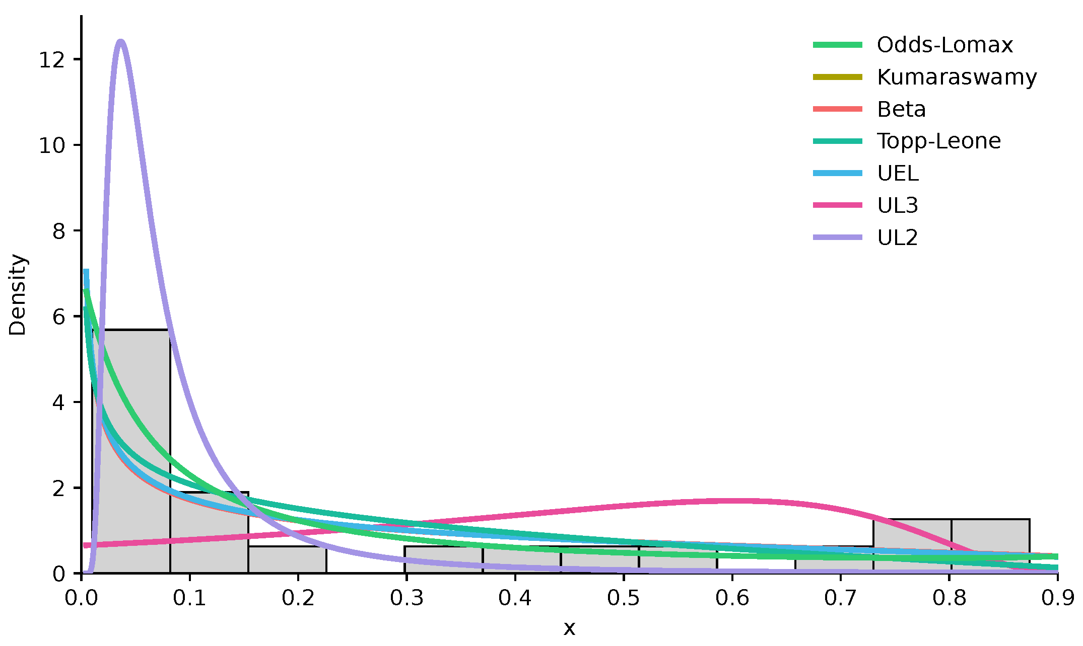
6.3. Dataset 1

Results for Dataset 1 are reported in

Table 5. Fitted models for Dataset 1. Reported are the estimated parameters with standard errors in parentheses, log-likelihood, AIC, BIC, and the KS statistic with parametric bootstrap p-value obtained after refitting the model in each bootstrap sample.

Model	Estimated Parameters (SE)	logLik	AIC	BIC	KS (p-Value)
odds-Lomax	$\alpha =0.5287$(0.1740)	10.7166	$-17.4331$	$-15.1621$	0.1154(0.4875)
	$\beta =0.0503\left(0.0370\right)$
Kumaraswamy	$\alpha =0.5044$(0.1288)	9.6708	$-15.3416$	$-13.0706$	0.1790(0.0619)
	$\beta =1.1862\left(0.3265\right)$
Beta	$\alpha =0.4869\left(0.1208\right)$	9.6075	$-15.2149$	$-12.9439$	0.1836(0.0809)
	$\beta =1.1679\left(0.3578\right)$
Topp-Leone	$\alpha =0.5943\left(0.1239\right)$	8.1151	$-14.2302$	$-13.0948$	0.1690(0.2617)
UEL	$\delta$ = 1,995,226,724.5142(38,034,025,245.5923)	9.6708	$-13.3416$	$-9.9351$	0.1790(0.0420)
	$\lambda \approx 0\left(\mathrm{boundary}\right)$
	$\eta =1.1861\left(0.3264\right)$
UL3	$\theta =1.2533\left(0.2010\right)$	$-6.8273$	15.6546	16.7901	0.4755(0.0010)
UL2	$\theta =0.0694\left(0.0102\right)$	$-16.8663$	35.7326	36.8681	0.4024(0.0010)

Note: The exceptionally large standard error for the UEL $\delta$ parameter reflects the numerical instability and boundary collapse discussed in Section 6.3.

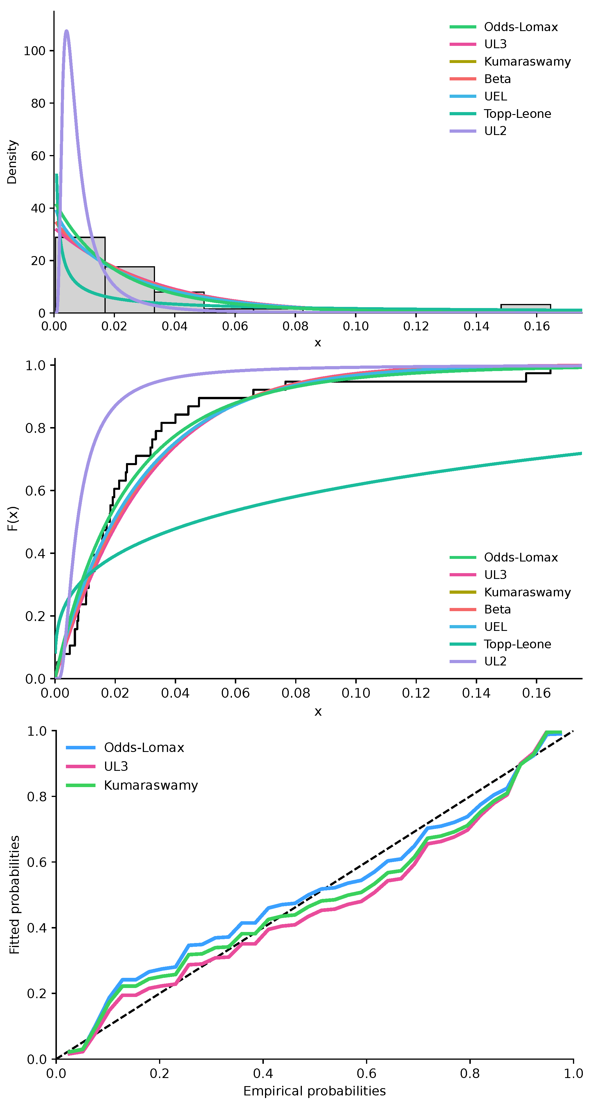
and illustrated in Figure 2. The odds-Lomax model provides the most favorable likelihood-based fit among the models considered, according to the log-likelihood, AIC, and BIC. The KS statistic and the bootstrap p-value are also consistent with an adequate fit. The Kumaraswamy and beta distributions remain competitive, whereas UL2 and UL3 show clearer signs of misspecification. The inclusion of the UEL model is especially relevant here because it represents the closest Lomax-based competitor. However, its fitted values suggest numerical instability, with one parameter effectively collapsing to the boundary of the parameter space. Accordingly, the UEL fit should be interpreted with caution in this dataset, and the present comparison supports the odds-Lomax model primarily in terms of relative fit and numerical stability under the current sample.

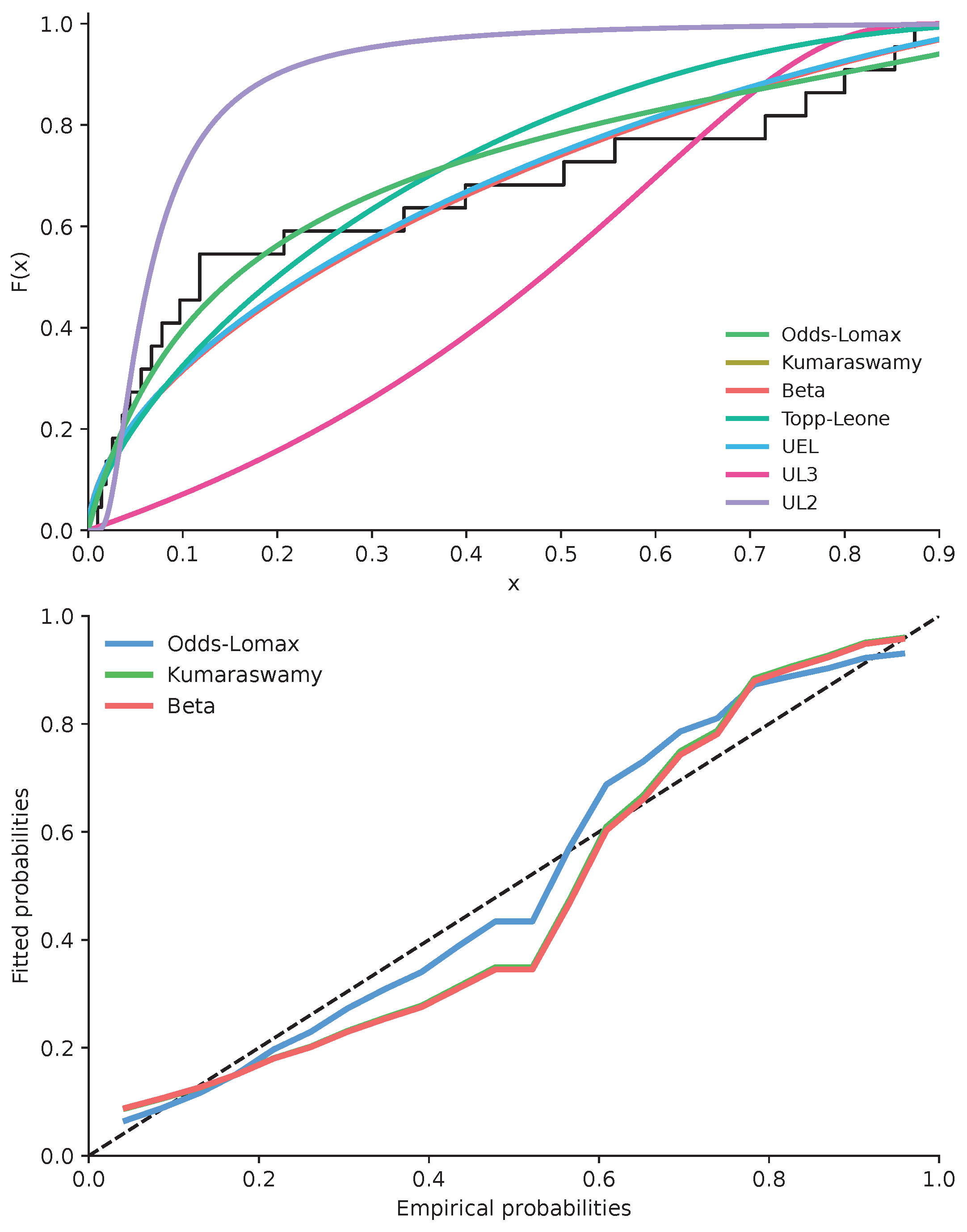
Graphical diagnostics provide more detailed support for these conclusions. The histogram with fitted densities shows a pronounced concentration of observations near zero together with a sparse right tail. In this panel, the odds-Lomax curve reproduces the overall decreasing pattern more closely than the competing models, whereas UL2 concentrates too much density near the lower boundary, and UL3 concentrates too much density over the middle and upper parts of the support. The empirical-versus-fitted CDF panel also favors the proposed model, whose curve tracks the empirical step function more closely over the lower and central portions of the sample. Finally, in the P-P plot, the odds-Lomax model remains closest to the 45-degree reference line, with only mild deviations in the middle-to-upper probability range, indicating a satisfactory global fit over the unit interval.

6.4. Dataset 2

Results for Dataset 2 are presented in

Table 6. Fitted models for Dataset 2. Reported are the estimated parameters with standard errors in parentheses, log-likelihood, AIC, BIC, and the KS statistic with parametric bootstrap p-value obtained after refitting the model in each bootstrap sample.

Model	Estimated Parameters (SE)	logLik	AIC	BIC	KS (p-Value)
odds-Lomax	$\alpha =0.6032$(0.2106)	7.9054	$-11.8108$	$-9.6287$	0.1112(0.5934)
	$\beta =0.0852\left(0.0626\right)$
Kumaraswamy	$\alpha =0.5718\left(0.1478\right)$	6.8436	$-9.6872$	$-7.5051$	0.1963(0.0350)
	$\beta =1.2305\left(0.3483\right)$
Beta	$\alpha =0.5540\left(0.1423\right)$	6.7819	$-9.5638$	$-7.3818$	0.2002(0.0380)
	$\beta =1.2198\left(0.3758\right)$
Topp-Leone	$\alpha =0.6778\left(0.1445\right)$	5.4983	$-8.9965$	$-7.9055$	0.1848(0.1728)
UEL	$\delta$ = 33,696,322.5669(NA)	6.8436	$-7.6872$	$-4.4141$	0.1963(0.0250)
	$\lambda \approx 0\left(\mathrm{boundary}\right)$
	$\eta =1.2305\left(0.3483\right)$
UL3	$\theta =1.1930\left(0.1948\right)$	$-6.5826$	15.1652	16.2562	0.4600(0.0010)
UL2	$\theta =0.1089\left(0.0165\right)$	$-10.6815$	23.3631	24.4541	0.3715(0.0010)

and Figure 3. Again, the odds-Lomax distribution provides the most favorable likelihood-based fit among the fitted competitors and is also supported by the KS-based evidence. The comparison with the UEL model is informative, but it also reveals a numerical issue: the UEL estimates approach the boundary of the parameter space, and some reported standard errors are unavailable. This behavior suggests weak local identifiability or instability of the Wald approximation for that model under the present dataset. Hence, although UEL is retained as an important Lomax-based benchmark, its fitted results should be interpreted with these limitations in mind.

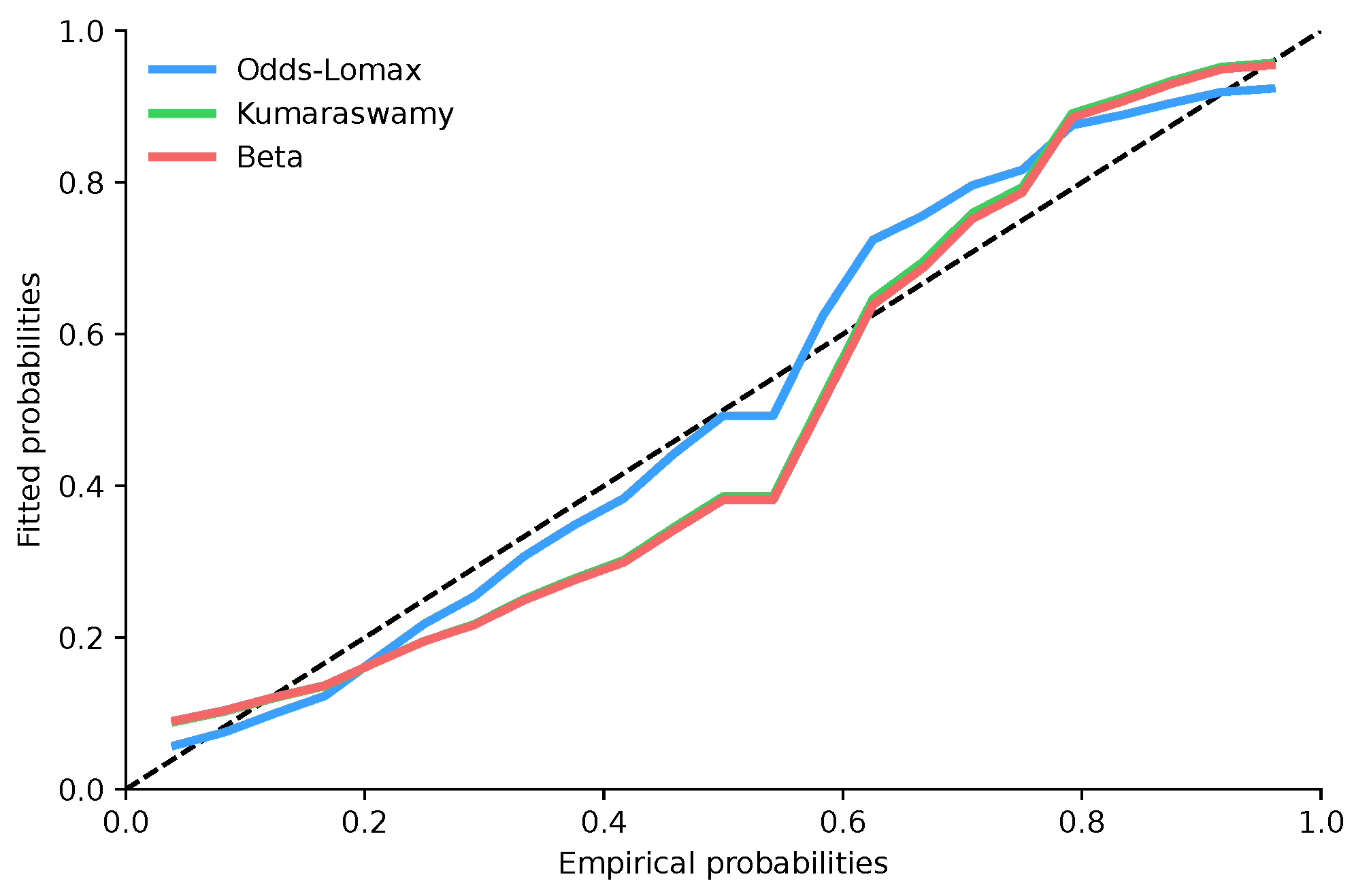
The graphical diagnostics reinforce this ranking. The histogram with fitted densities again reveals a marked concentration near zero, and the odds-Lomax density follows this shape more convincingly than the main competitors, while UL2 and UL3 display a clear mismatch in body and tail behavior. In the empirical-versus-fitted CDF panel, the proposed model remains closer to the empirical distribution over most of the support, especially in the lower and intermediate regions where an accurate fit is most important for this dataset. The P-P plot confirms this visual advantage: the odds-Lomax curve stays closest to the diagonal benchmark, whereas the beta and Kumaraswamy models show more systematic departures. Although the UEL curve is visually competitive in parts of the support, its numerical instability prevents a reliable inferential interpretation.

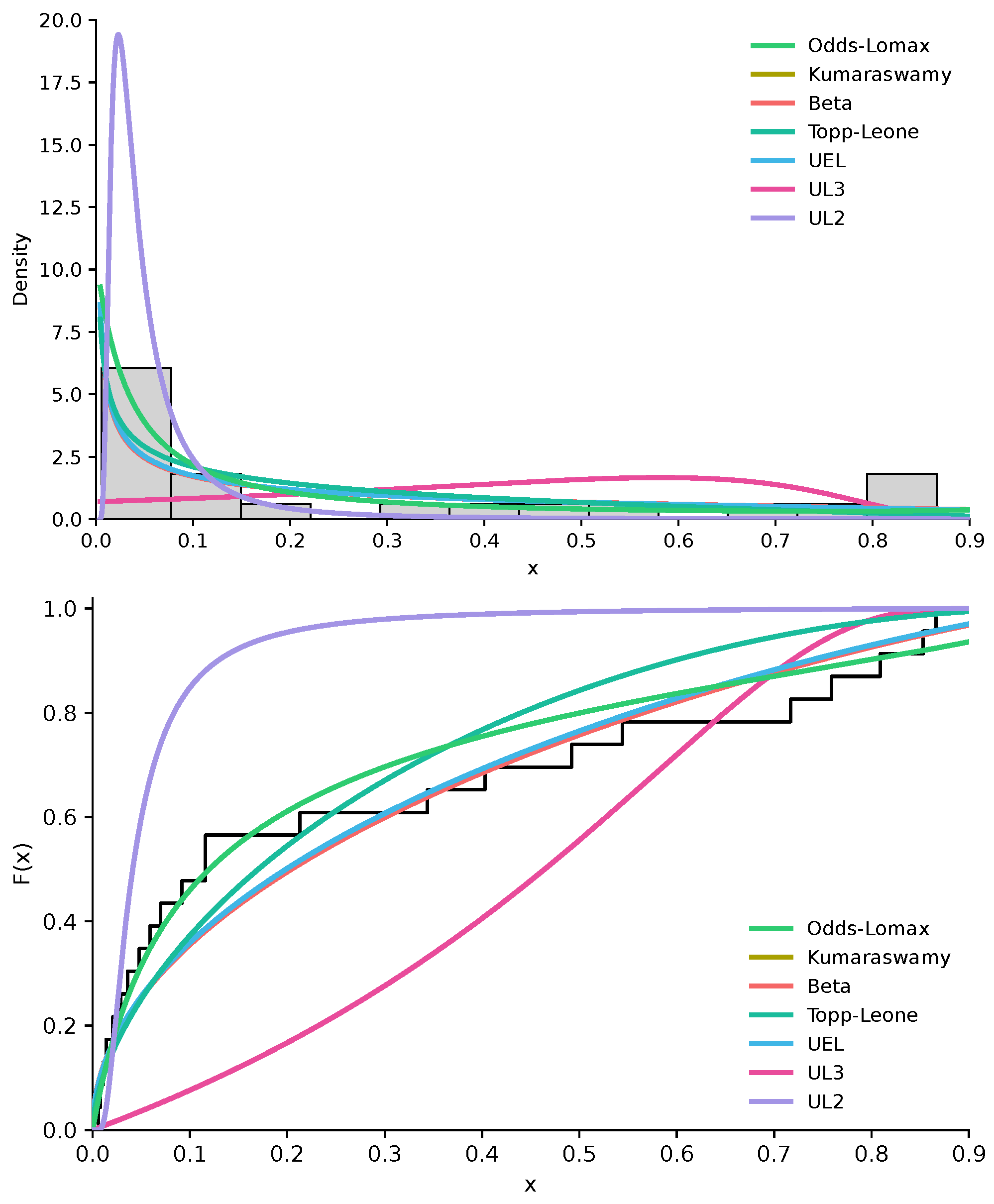
6.5. Dataset 3

The results for Dataset 3 are shown in

Table 7. Fitted models for Dataset 3. Reported are the estimated parameters with standard errors in parentheses, log-likelihood, AIC, BIC, and the KS statistic with parametric bootstrap p-value obtained after refitting the model in each bootstrap sample.

Model	Estimated Parameters (SE)	logLik	AIC	BIC	KS (p-Value)
odds-Lomax	$\alpha =4.2092$(3.0631)	98.1216	$-192.2432$	$-188.9680$	0.1361(0.0689)
	$\beta =0.0979\left(0.0860\right)$
Kumaraswamy	$\alpha =0.9407\left(0.1180\right)$	97.1480	$-190.2959$	$-187.0207$	0.1169(0.1828)
	$\beta =28.1415\left(11.4977\right)$
Beta	$\alpha =0.9799\left(0.1976\right)$	97.0289	$-190.0578$	$-186.7826$	0.1224(0.1918)
	$\beta =33.2395\left(8.5587\right)$
UEL	$\delta$ = 82,309,105.2602(82,698,606.4643)	97.1480	$-188.2959$	$-183.3832$	0.1169(0.1548)
	$\lambda \approx 0\left(\mathrm{boundary}\right)$
	$\eta =28.1358\left(11.5207\right)$
Topp-Leone	$\alpha =0.2898\left(0.0470\right)$	71.2670	$-140.5340$	$-138.8964$	0.3919(0.0010)
UL3	$\theta =33.5019\left(5.2858\right)$	96.5835	$-191.1669$	$-189.5293$	0.1350(0.2138)
UL2	$\theta =0.0125\left(0.0014\right)$	61.4598	$-120.9196$	$-119.2820$	0.4221(0.0010)

and Figure 4. This dataset presents a more challenging structure due to the strong concentration of observations near zero. The odds-Lomax model remains highly competitive according to the likelihood-based criteria, while alternative models such as UL3 and Kumaraswamy exhibit competitive behavior in some diagnostic aspects. The UEL model again yields estimates close to the boundary, indicating that its numerical fit is comparatively unstable for this dataset. Therefore, although it remains a natural Lomax-based comparator, the practical interpretation of its parameter estimates and standard errors is limited in this case.

The graphical diagnostics show why this dataset is more difficult. The histogram with fitted densities indicates a very strong concentration near zero, together with a thin but non-negligible spread over the remaining support. In this panel, no single competitor dominates uniformly: some alternative models adapt reasonably well in restricted regions, but the odds-Lomax density provides a more balanced representation of the sharp lower-tail behavior and the subsequent decay. The empirical-versus-fitted CDF panel shows a similar behaviour. While several curves remain close to the empirical step function, the proposed model maintains good agreement across most of the support without the pronounced distortions displayed by the clearly misspecified models. The P-P plot further indicates that the comparison is tighter than in Datasets 1 and 2, since Kumaraswamy and UL3 also track the empirical probabilities reasonably well. Even so, the odds-Lomax model preserves the best overall compromise between lower-tail adaptation, global fit, and consistency with the likelihood-based criteria.

The bootstrap intervals in

Table 8. Parametric bootstrap percentile intervals for the MPS estimator in the empirical datasets.

Dataset	n	${\widehat{\mathit{\alpha }}}_{\mathbf{MPS}}$	${\widehat{\mathit{\beta }}}_{\mathbf{MPS}}$	${\mathit{CI}}_{\mathit{\alpha },\mathit{L}}^{\mathbf{boot}}$	${\mathit{CI}}_{\mathit{\alpha },\mathit{U}}^{\mathbf{boot}}$	${\mathit{CI}}_{\mathit{\beta },\mathit{L}}^{\mathbf{boot}}$	${\mathit{CI}}_{\mathit{\beta },\mathit{U}}^{\mathbf{boot}}$
SC16	23	0.42332	0.03122	0.22756	0.79129	0.00560	0.11054
P3	22	0.47686	0.05444	0.24868	0.94280	0.00948	0.23064
BLI	38	2.82966	0.06556	1.03106	1050.95670	0.01368	27.15812

should be interpreted as complementary finite-sample diagnostics rather than as replacements for the Hessian-based intervals. For the SC16 and P3 datasets, the bootstrap intervals are relatively moderate and support the use of MPS as a stable, robustness-oriented alternative. For the BLI dataset, however, the bootstrap interval for $\alpha$ is very wide, indicating substantial finite-sample uncertainty. This reinforces the need to interpret parameter estimates cautiously when the sample is small, strongly asymmetric, or highly concentrated near a boundary.

6.6. Overall Assessment

The empirical applications should be interpreted primarily as illustrative examples rather than as definitive evidence of estimator superiority. This caution is particularly relevant for Datasets 1 and 2, whose sample sizes are small, with $n=23$ and $n=22$, respectively. Although these datasets are useful for illustrating the behavior of the odds-Lomax model on bounded performance-type data, small samples may lead to unstable estimates, inflated standard errors, and wide confidence intervals. Therefore, the empirical results are interpreted together with the simulation study and the stability diagnostics reported in Table 4.

Some fitted models produce relatively large standard errors and wide confidence intervals, especially in small-sample settings or when the data are highly concentrated near the boundary of the unit interval. These cases should not be interpreted as strong empirical evidence in favor of a particular estimator or model. Rather, they provide empirical manifestations of the same instability mechanisms identified in the simulation study: observations close to one are mapped into large odds-scale values, which may flatten or ill-condition the objective function. For this reason, large standard errors, wide intervals, high Hessian condition numbers, and small minimum Hessian eigenvalues are interpreted as warning signals. In such cases, MPS estimates, bootstrap intervals, and the stability diagnostics in Table 3 and Table 4 are reported as complementary tools for assessing the numerical stability and inferential validity of the fitted results.

Across the three datasets, the odds-Lomax distribution provides a competitive fit relative to the bounded-data models considered here. The model is particularly useful when the data exhibit marked asymmetry or concentration near one of the endpoints. The comparison with the unit exponentiated Lomax model is especially relevant because it represents a close Lomax-based competitor. In the present applications, the odds-Lomax fits were numerically interpretable and did not exhibit the boundary-estimation problems observed for some competing models. However, in view of the Monte Carlo results, this empirical stability should be interpreted as dataset-specific rather than as a general guarantee of uniform MLE stability.

6.7. Discussion of Empirical Results

The empirical analysis across the three datasets highlights both the flexibility and the limitations of the proposed formulation. In Datasets 1 and 2, the histogram panels show that the odds-Lomax model captures the strong concentration of observations near the lower part of the unit interval, while the empirical-versus-fitted CDF plots indicate close agreement with the observed distribution over most of the support. The corresponding P–P plots show only minor deviations from the diagonal reference line, which is consistent with the favorable goodness-of-fit statistics.

For Dataset 3, the graphical comparison is more nuanced. The histogram and fitted-density panel reveal a more difficult tail structure, and some competitors remain visually close to the proposed model in restricted regions of the support. Nevertheless, when numerical fit criteria, graphical diagnostics, and interpretability are considered jointly, the odds-Lomax model remains a competitive option.

These applications should be read together with the simulation study. While the fitted examples indicate that the odds-Lomax model can be useful in practice, the Monte Carlo results show that standard MLE may be unstable in small-sample or heavy-tailed regimes. Therefore, in empirical work, likelihood estimates should be accompanied by convergence diagnostics, interval-length checks, and, when necessary, alternative estimation methods such as MPS.

7. Conclusions

This paper has provided a structural, inferential, and computational study of an odds-Lomax model on $(0,1)$ induced by the transformation $Z=Y/(1+Y)$ with $Y\sim \mathrm{Lomax}(\alpha ,\beta )$. A central contribution is the explicit clarification of the relationship between this odds-scale formulation and previously used unit-Lomax-type constructions. In particular, the model is not presented as a genuinely new distributional family, but rather as an odds-scale representation that is equivalent, up to complementation and reparametrization, to an existing Lomax-based unit construction. This clarification helps resolve issues of parametrization and nomenclature while preserving a direct probabilistic interpretation in terms of a heavy-tailed latent variable.

The model retains substantial analytical tractability. Closed-form expressions were obtained for the main distributional functions, quantile function, hazard rate, endpoint behavior, and stochastic representations. Moment and entropy-related quantities can also be evaluated through tractable formulas involving standard special functions or stable numerical procedures.

From an inferential perspective, the odds transformation shows that likelihood inference for the unit-interval model reduces to classical Lomax inference on the transformed sample $Y_i=Z_i/(1-Z_i)$. This representation is useful computationally, but it also explains the finite-sample instability of the MLE in heavy-tailed regimes. Observations close to the upper boundary of the unit interval generate extreme values on the odds scale, which may lead to flat likelihood surfaces, ill-conditioned observed information matrices, inflated Wald intervals, and very large RMSE values.

The Monte Carlo study therefore provides a more nuanced conclusion than a standard likelihood analysis alone. The MLE performs satisfactorily in several moderate-tail configurations and sufficiently large samples, but its reliability is not uniform over the entire parameter space. The simulation results show that isolated extreme estimates may still occur for some parameter combinations, making interval-length checks, MedAE, and comparison with MPS essential diagnostic tools.

The empirical applications show that the odds-Lomax formulation can be competitive for bounded data exhibiting asymmetry or endpoint concentration. However, the practical use of the model should be accompanied by diagnostic checks, including convergence assessment, interval-length inspection, and comparison between MLE and MPS estimates when the data suggest heavy-tailed behavior on the odds scale.

Future work may consider regression extensions, multivariate constructions on the simplex, copula-based dependence structures, profile-likelihood or bootstrap interval estimation, and systematic comparisons between likelihood-based, spacing-based, and fiducial procedures for bounded data.