Article

Replacing the Genetic Algorithm with Multi-Objective Bacterial Foraging Optimization in XCS

Institute of Informatics, Faculty of Electrical Engineering and Computer Science, University of Maribor, Koroška Cesta 46, 2000 Maribor, Slovenia
*
Author to whom correspondence should be addressed.
Mathematics 2026, 14(11), 1947; https://doi.org/10.3390/math14111947
Submission received: 4 May 2026 / Revised: 25 May 2026 / Accepted: 31 May 2026 / Published: 2 June 2026
(This article belongs to the Special Issue Swarm Intelligence and Optimization: Algorithms and Applications)

Highlights

What are the main findings?
  • BFOA replaces GA in XCS, creating a novel classifier optimization system that evaluates multiple fitness criteria simultaneously through a weighted sum scalarization.
  • BFOA enables concurrent optimization of classifier accuracy, stability, and variance.
  • BFOA-XCS achieves the top Friedman ranking among XCS variants across 19 benchmark datasets, with notable variance reduction (15.2%) over standard GA-XCS.
  • In dynamic cybersecurity defense, XCS variants significantly outperform three of five deep RL baselines (DQN, Q-Learning, Policy Gradient (REINFORCE)), while PPO and SAC achieve higher overall rewards at substantially higher computational cost.
What are the implications of the main findings?
  • Swarm intelligence offers a viable alternative to evolutionary operators in LCS research.
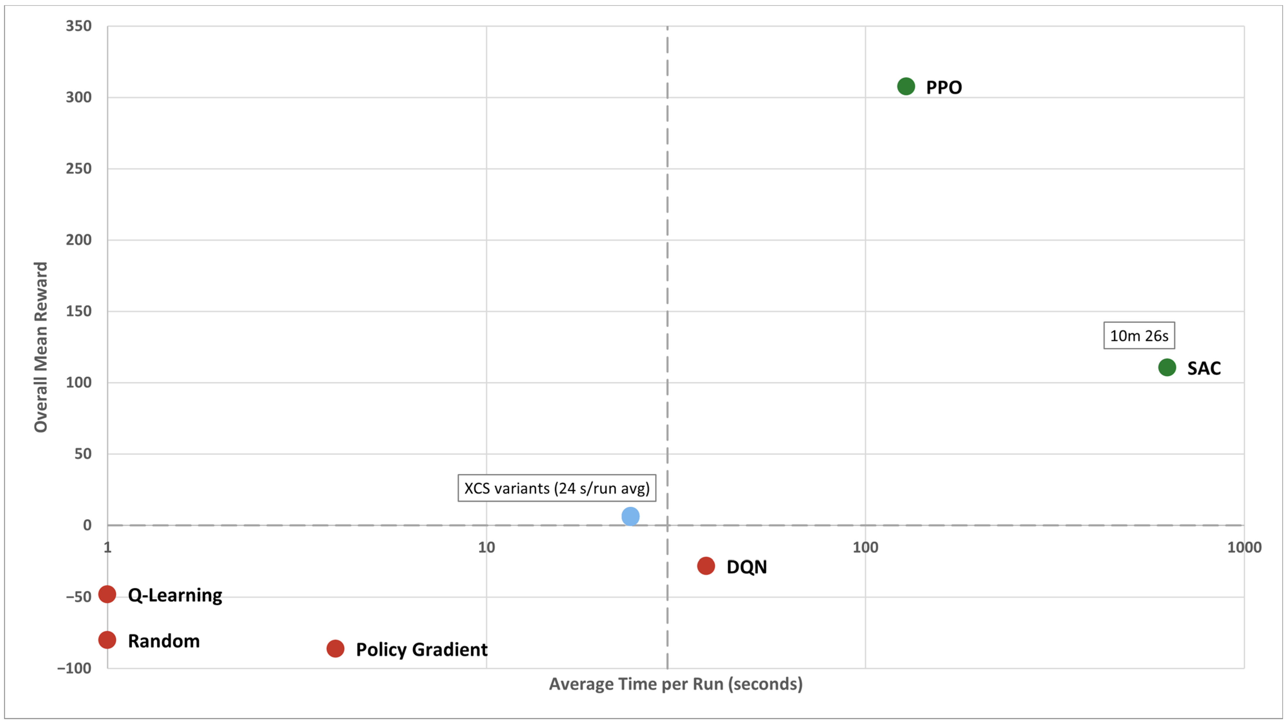
  • Rule-based XCS provides competitive cybersecurity defense with interpretable policies, warmup-free competence, and 5–26× lower computational overhead compared to the top-performing neural approaches (PPO at 5.3× and SAC at 26.1× the XCS compute time per training run).
  • The BFOA-XCS hybrid generalizes across diverse static and dynamic environments.

Abstract

This article is positioned into a cross-section of machine learning, cybersecurity, and nature-inspired domains. This article’s main objective is to use eXtended Classifier System (XCS), a known adaptive Reinforcement Learning (RL) algorithm, and alter it to use the Bacterial Foraging Optimization Algorithm (BFOA) instead of its original Genetic Algorithm component. This modification transforms XCS into a multi-criteria optimization system (BFOA-XCS) through evaluation of classifier fitness across accuracy, stability, and variance reduction while simultaneously using weighted-sum scalarization. In this way, the method leverages BFOA’s chemotactic search and population dynamics. The proposed BFOA-XCS integration was validated in two experimental phases. First, evaluations across 19 benchmark machine learning datasets demonstrated that Improved BFOA (IBFOA)-XCS achieves the best Friedman ranking among all XCS variants (marginally significant at α = 0.10, supported by medium-to-large effect sizes), with notable variance reduction (15.2 percent) over standard GA-XCS. Second, in a dynamic cybersecurity simulation environment with six attack scenarios, all XCS variants significantly outperformed three of five deep RL baselines (Deep Q-Network (DQN), Q-Learning, and Policy Gradient (REINFORCE)) with large statistical effect sizes. Proximal Policy Optimization (PPO) and Soft Actor–Critic (SAC) achieved higher overall rewards but at substantially greater computational cost: PPO at 5.3× and SAC at 26.1× the XCS compute time per run (2 min 8 s and 10 min 26 s, respectively, vs. 24 s for XCS). The results demonstrate that rule-based XCS with BFOA optimization offers a compelling alternative to neural approaches for cybersecurity defense, combining competitive performance with interpretable policies and substantially lower computational requirements.

1. Introduction

The modern world runs on the power of knowledge provided by information and technology [1], which are crucial for different social, biological, and economic systems. Technology systems that enable such modern operations heavily rely on the leading artificial intelligence technology [2]. Specifically, computer research fields of computational intelligence, machine learning (e.g., Reinforcement Learning (RL) adaptive systems), and nature-inspired systems [3], the cross-section of which our work is positioned, are playing an essential role in tackling an ever-increasing complexity of the world of information.
In 1976 [4], Holland introduced foundational ideas in adaptation and evolutionary computation that later influenced Learning Classifier Systems (LCS). Even after many decades, these systems are still the subject of intense research [5]. The first LCS architecture was Cognitive System One (CS-1) [6], which utilizes two main components: RL, where the system learns based on the rewards received when executing actions in the environment, and evolutionary mechanisms. Now, the eXtended Classifier System (XCS) [7] is one of the most known and investigated algorithms in the LCS group [8]. The XCS population presents a model-free solution to the problem when it has evolved (i.e., the learning process has been completed). It is structured as a set of classifiers (population), where a classifier can be seen as an “if condition then action” structure. The condition is usually a binary representation of the (part of) environment (e.g., large-scale dynamic IoT environment [9]), and the action is a viable choice a system can perform in that environment (e.g., control inputs (actions) for a spherical robot [10]).
The pioneered evolutionary, nature-based Genetic Algorithm (GA) optimization component first introduced in CS-1 was crucial to its operation. Today, the GA is integral to many algorithms from the LCS group, and the field has also evolved into a world-known standalone research domain. But the GA from the group of evolutionary-based algorithms (e.g., another well-known algorithm from this group is differential evolution [11]) is not the only viable optimization solution. There are many other metaheuristic algorithm groups with various valuable options. Groups such as Swarm-based algorithms (SBA) (e.g., ant colony optimization [12]), Physics/Chemistry-based algorithms (e.g., black hole algorithm [13]), Human-based Algorithms (e.g., teaching–learning-based optimization [14]), Ecosystem-based algorithms (e.g., artificial ecosystem-based optimization [15]), to name just a few, can be utilized. The pool of choices is vast [16] because solving both artificial benchmarks and real-world engineering problems requires a diverse set of techniques, as implied by the No Free Lunch theorems (i.e., no single optimization algorithm performs best across all problem classes) [17].
In this work, the Bacterial Foraging Optimization Algorithm (BFOA) is utilized, which mimics the collective foraging behavior of bacteria and, therefore, belongs to the SBA group of nature-based optimization algorithms [18]. The selection of the BFOA algorithm was carefully considered, taking multiple factors into account. The first consideration was to use the algorithm, which would be a worthy substitute for the GA component [19] found in the XCS algorithm. For example, current research is promising, and modified BFOA has been found to have a greater convergence speed than the original GA in the real-problem industry setting [20]. The second consideration was to have an algorithm with great local and global optimization ability [21] (i.e., with the main line of thought being that the movement mechanisms of bacteria in BFOA would serve exceptionally well for (local) action adaptivity). The third consideration was to avoid GA’s sensitivity to the initial selection of its hyperparameter values (i.e., evolutionary algorithms are sensitive to correct initial settings [22]) and its premature convergence [23] to suboptimal solutions due to loss of genetic diversity).
The main contributions of this article are as follows:
  • Replacing the GA component in XCS with BFOA, extending the LCS research domain with a bio-inspired swarm intelligence algorithm. To the best of the authors’ knowledge, this is the first integration of BFOA with the LCS. The integration pattern itself is independent of the specific swarm optimizer chosen. BFOA is one instantiation, and the same template can in principle accommodate other population-based optimizers.
  • Introducing a weighted multi-criteria fitness function that leverages BFOA’s population dynamics to simultaneously evaluate classifier accuracy, prediction stability, and variance reduction. These capabilities were not natively supported by the standard single-objective GA operator, which evaluates and recombines classifiers in pairs rather than as a coordinated population.
  • Comprehensive empirical validation across two experimental domains: static classification on 19 machine learning datasets and dynamic cybersecurity defense in a simulated network environment with six distinct attack scenarios, demonstrating that BFOA-XCS achieves consistent ranking improvements over standard XCS, supported by medium-to-large effect sizes (Cohen’s d = 0.623–0.803) and a 15.2% variance reduction.
  • Comparative evaluation against modern deep RL (DRL) baselines (Deep Q-Network (DQN), Q-Learning, Policy Gradient (REINFORCE), Proximal Policy Optimization (PPO), and Soft Actor–Critic (SAC)), demonstrating that XCS with BFOA optimization significantly outperforms three of five neural baselines (DQN, Q-Learning, and Policy Gradient) while offering interpretable decision rules, warmup-free competence, and substantially lower computational cost per training run than the top-performing neural agents (PPO at 5.3× and SAC at 26.1× the XCS compute time).
Throughout this article, BFOA-XCS refers jointly to all XCS variants utilizing BFOA-based optimization, including standard BFOA, Adaptive BFOA, and Improved BFOA (IBFOA), unless a specific variant is indicated.
This article’s structure is as follows. Section 2 presents relevant works related to the domains of LCS and nature-inspired heuristics. Section 3 describes the methods and methodology, detailing the XCS algorithm, the BFOA variants, their integration (BFOA-XCS), and the cybersecurity simulation environment. Section 4.1 presents Experiment 1 on benchmark machine learning datasets and reports the statistical analyses of operator performance. Section 4.2 presents Experiment 2 in the dynamic cybersecurity defense setting and compares XCS variants against DRL baselines. Section 5 discusses the interpretation of results and this study’s limitations. Section 6 outlines directions for future work. Finally, Section 7 concludes the article.

2. Related Domains

This section provides a brief overview of the LCS domain, specifically the XCS subdomain and the Nature-Inspired Metaheuristics domain, with a focus on the works related to the BFOA.

2.1. Learning Classifier Systems: The eXtended Classifier Systems Subdomain

LCS is a group of rule-based algorithms that can be built upon and draw from the cross-section of domains such as RL [24], Q-Learning [25], R-Learning [26], evolutionary optimization [27], and many others. The word ‘can’ is used to emphasize that not all algorithms within the LCS group employ all these techniques at the same time. LCSs are utilized in the applicative fields ranging from data mining [28] to aviation management [29], across different tasks such as classifications [30] or domains of imperfect information [31].
Over the decades, the research field of LCS has matured from the CS-1 algorithm into two main groups called Pittsburgh and Michigan style [27,32]. The Pittsburgh style evolves a population of complete rule sets (i.e., the whole set is the solution) [33]. In contrast, the Michigan style evolves individual rules within a population, enabling rule-level specialization and adaptation [34]. The LCS group now holds many algorithm sub-branches. Most notable is XCS, which is most widely used and belongs to the Michigan style [35], while others range from relatively simple systems such as the zeroth level classifier system (ZCS) [36]; powerful eXtended Classifier System with Function Approximation [37], which can approximate complex multi-dimensional function surfaces by utilization a mosaic of simpler functions; and Anticipatory Learning Classifier Systems, which also meets the criteria for eXplainable Artificial Intelligence [38].
The current open research directions in XCS are extensive. For example, there is a constant need for research on advanced classifier representations [39]. Another field of research belongs to memory-based XCS systems, which have shown promise in improving the efficiency of rule discovery and application, in complex real-world scenarios, such as maze navigation and traffic problems in wireless networks [40]. One of the essential focuses of the research is also the evolutionary process [41]. It can be argued that the optimizer is essential, but so far, it has not been researched as much as LCS’s learning components [42]. Therefore, a need for further research advancements in the XCS evolutionary process, as in this work, is a logical (evolutionary) step.

2.2. Nature-Inspired Metaheuristic: Bacterial Foraging Optimization Algorithm

Nature-inspired metaheuristic algorithms are optimization techniques that model natural systems and have seen a worthy rise in research in recent years [43]. By mimicking biological and physical processes, these algorithms efficiently solve complex problems and can be classified by their inspiration sources (e.g., bio-based, ecosystem-based, social-based, physics-based, chemistry-based, mathematics-based, and hybrid families) [44]. Among these, the BFOA stands out as a notable example of an SBA group.
Escherichia coli is one of the most well-studied bacterial species and is commonly found as a member of the healthy human gut microbiome [45]. The BFOA, as the name suggests, is based on bacterial foraging behavior, which is also known as chemotaxis [46], and in simple terms describes bacterial movements directed towards beneficial chemicals (stimulus) [47] while avoiding harmful substances. Other steps of the BFOA algorithm cover bacterial reproduction, swarming, elimination, and dispersal, which are described in more detail in Section 3, and are under constant research improvements. For example, IBFOA, which enhances both the chemotaxis and elimination–dispersal mechanisms, has been shown to outperform the original BFOA in terms of convergence speed and accuracy [48].
The selection of BFOA for the present work is grounded in two structural properties of the algorithm that align with the requirements of the XCS classifier population. First, BFOA’s chemotactic step generates small, continuous-valued displacements by the tumble-and-swim mechanism, which makes it well suited for detailed refinement of classifier action parameters once XCS has produced a candidate population, without disrupting the binary condition representation that XCS relies on for state matching. Second, BFOA evaluates a population of bacteria as a coordinated whole at each chemotactic iteration, which enables a multi-criteria fitness function (Section 3.3.2) to be assessed at the population level, a property that the standard GA, with its pairwise crossover and mutation semantics, does not natively support. These two properties motivate the integration mechanism proposed in Section 3.3. The integration pattern itself is independent of the specific swarm optimizer chosen; comparative evaluation of more recent swarm or evolutionary alternatives instantiated under the same template is a natural direction for future work.

2.3. Reinforcement Learning in Cybersecurity

The intersection between RL and cybersecurity is a fast-developing research area because cyber threats grow in sophistication and frequency [49]. Traditional defense mechanisms based on rule- or signature-based detection, along with static firewall rules, are increasingly insufficient [50]. Approaches that utilize RL offer the ability to adapt and respond to dynamic threat environments in real time, making them attractive for autonomous cyber defense [51].
DRL is one of the dominant computational approaches within cybersecurity. DRL methods such as DQN have been applied to intrusion detection [52], vulnerability management [53], and automated threat response [54]. More advanced architectures have also been explored, ranging from actor–critic methods, such as PPO and SAC for multi-step defense scenarios [55], to multi-agent-inspired and federated RL frameworks designed to protect large-scale network infrastructures [56].
Despite this progress, the existing body of work is dominated by neural network-based approaches. Rule-based learning systems, which offer inherent interpretability (a property that is highly desirable and useful in security-critical domains where understanding the rationale behind defensive decisions is essential), remain largely unexplored in this context. While only limited works have applied LCS variants to intrusion detection as a classification task [57], the use of LCS as an adaptive RL agent for closed-loop, dynamic network defense remains largely unexplored.
Furthermore, to the best of our knowledge, prior cybersecurity uses of LCS have not progressed beyond the standard GA evolutionary component, and the combination of LCS with other nature-inspired optimizers therefore appears underexplored in cybersecurity settings. This gap is particularly important because cybersecurity defense environments often exhibit large, structured, discrete action spaces, where rule-based representations can provide interpretable, modular decision structures. By contrast, many deep RL approaches typically rely on neural function approximation for value/policy estimation, which may trade interpretability for representational power.
In the next section, a transition is made from an overview of the related research domains to a detailed examination of the methods, including the operational mechanisms of XCS and BFOA, their integration, and the cybersecurity simulation environment.

3. Methods and Methodology

This section presents the methods and methodology behind the proposed BFOA-XCS system. It begins with a description of the XCS algorithm and its main execution cycle, followed by the BFOA and its variants. The integration of BFOA into XCS, including the multi-objective classifier fitness function, is also explained in detail. This section concludes with a description of the cybersecurity simulation environment designed for the experimental evaluation.

3.1. eXtended Classifier System

The XCS algorithm is a rich learning framework that combines adaptivity, generalization, and scalability. Its RL component uses a Q-learning-style temporal-difference update [58], although alternative formulations such as R-learning have also been shown viable [26]. These properties make XCS a versatile algorithm within the LCS family.
The XCS algorithm used in this research was implemented manually, line by line transformation from the pseudocode to Java code, following the original algorithmic description by Butz and Wilson [58]. No external libraries or code generation tools were used for the XCS implementation and its GA component.

3.1.1. Knowledge Representation

XCS has knowledge represented through utilization of classifiers organized in four sets. The population [P] contains all classifiers that exist at a given time step t and represents the system’s accumulated knowledge about the problem. The match set [M] is formed by selecting all classifiers from [P] whose conditions match the current environmental state σ. The action set [A] is a subset of [M] containing all classifiers that advocate the action selected for execution, and the [A]−1 is a copy of the action set from the previous time step, used for multi-step problems where reward assignment must be propagated backward through sequential decisions.
Each classifier consists of a condition (typically a binary string with don’t-care symbols ‘#’), an action, and several parameters: the reward prediction p, the prediction error ε, the fitness F, the experience exp, the numerosity num, and the time stamp ts of the last GA invocation. The don’t-care symbol ‘#’ enables generalization. A classifier with more ‘#’ symbols in its condition matches a wider set of environmental states, allowing XCS to discover maximally general but accurate rules.

3.1.2. Main XCS Cycle

The main operational cycle of XCS is presented in Algorithm 1.
Algorithm 1 Pseudocode of the XCS main reinforcement learning cycle (adapted from [58])
initialize reinforcement_program rp
initialize environment env
initialize XCS    // create population [P]; connect to evaluation function
procedure RUN_XCS()
    1. do {
    2.      σ = get sensory input from env
    3.      generate [M] from [P] using σ    // covering may be activated
    4.      generate PA from [M]
    5.      act = select action according to PA
    6.      execute act in env
    7.      ρ = get reward from rp
    8.      if [A]−1 is not empty then
    9.          P = ρ−1 + γ·max(PA)
  10.          update set [A]-1 using P, possibly deleting in [P]
  11.          → run GA in [A]−1, possibly inserting in [P] // replaced by BFOA (Section 3.3)
  12.      end if
  13.      if rp signals end-of-problem then
  14.          P = ρ
  15.          update set [A] using P, possibly deleting in [P]
  16.          → run GA in [A], possibly inserting in [P] // replaced by BFOA (Section 3.3)
  17.          clear [A]−1
  18.      else
  19.          [A]−1 = [A]
  20.          ρ−1 = ρ
  21.          σ−1 = σ
  22.      end if
  23. } while (termination criteria from rp are not met)
end procedure
The cycle begins by receiving sensory input σ from the environment (line 2). The match set [M] is formed from [P] using σ, with a covering mechanism activated if no classifiers match the current state (line 3). A prediction array PA is then computed from [M], aggregating the fitness-weighted predictions for each possible action (line 4). An action is selected according to PA, typically using a greedy strategy that balances exploration and exploitation (line 5). The selected action is executed in the environment (line 6), and a reward ρ is obtained from the reinforcement program (line 7).
If a previous action set [A]−1 exists (line 8), the system computes an update target P using the previous reward and the discounted maximum of the current prediction array (line 9, corresponding to Q-learning’s temporal difference update). The classifiers in [A]−1 are then updated using P, with deletion of excess classifiers possible in [P] (line 10). The genetic algorithm is then applied to [A]−1 (line 11), with offspring potentially inserted into [P]. When the reinforcement program signals the end of an episode (line 13), the current action set [A] is updated directly with the final reward (lines 14–16), and [A]−1 is cleared (line 17). Otherwise, the current state is stored for the next iteration (lines 19–21).
Lines 11 and 16 (marked with →) represent the evolutionary optimization step where, in standard XCS, the genetic algorithm is invoked. The GA is triggered only when the average time since its last invocation in the action set exceeds a threshold θGA. This evolutionary step is the component that is replaced by BFOA in the proposed BFOA-XCS system, as detailed in Section 3.3.

3.2. Bacterial Foraging Optimization Algorithm

In this section, the BFOA and the variants of this algorithm used in the experiments are described. First, the standard BFOA is introduced. Next, the Adaptive BFOA is outlined, followed by the IBFOA. In each case, specific mechanisms of the original algorithm are modified to address known limitations.

3.2.1. Standard BFOA

The BFOA, originally proposed by Passino [18], mimics the natural foraging behavior of Escherichia coli bacteria through several biologically inspired steps. Chemotaxis involves the movement of bacteria towards beneficial chemicals and away from harmful ones through a sequence of tumble (random direction change) and swim (continued movement in a successful direction) operations. The reproduction phase retains and multiplies the bacteria that perform best while replacing the weaker half of the population. Elimination and dispersal introduce diversity by randomly relocating bacteria with a fixed probability, preventing premature convergence to local optima. These steps are nested in a three-level loop structure that enables the algorithm to balance local exploitation (chemotaxis) with global exploration (elimination-dispersal).
There are numerous variations and interpretations of the BFOA since its original inception, and their pseudocode representations vary. For example, BFOA with added social learning, which directs bacteria to tumble towards better solutions in the chemotactic steps [59], or an enhanced BFOA variant employing a novel step-size evolution to overcome fixed step-size limitations and improve computing efficiency [60]. The pseudocode of Algorithm 2 therefore serves as an overview representation of the core concepts, effectively capturing the algorithm’s essential chemotaxis, reproduction, and elimination-dispersal processes as implemented in this work.
Algorithm 2 Pseudocode of the standard Bacterial Foraging Optimization Algorithm (based on [18])
Input:
N: Number of bacteria
Nc: Number of chemotactic steps
Nr: Number of reproduction steps
Ned: Number of elimination-dispersal steps
Ns: Swim length (max swim steps per tumble)
Pe: Probability of elimination
LB, UB: Search space bounds
F: Evaluation (fitness) function
Output: Best solution found
1.    Initialize N bacteria at random positions within [LB, UB]
2.    Evaluate health of each bacterium using F
3.    for ed = 1 to Ned do            // Elimination-Dispersal
4.        for rs = 1 to Nr do            // Reproduction
5.            for cs = 1 to Nc do           // Chemotaxis
6.                for each bacterium i do
7.                    Generate random tumble direction Δ
8.                    Normalize: φ = Δ/||Δ||
9.                    Move: xnew = xi + C·φ        // C = step size
10.                  Evaluate F(xnew)
11.                  if F(xnew) < F(xi) then        // Improvement found
12.                      xi = xnew            // Accept new position
13.                      for s = 1 to Ns do         // Swim in same direction
14.                          xswim = xi + C·φ
15.                          if F(xswim) < F(xi) then
16.                              xi = xswim
17.                          else break          // Stop swimming
18.                      end for
19.                  end if
20.              end for (bacterium)
21.          end for (chemotaxis)
22.          Sort bacteria by health (ascending)
23.          Replace worst N/2 bacteria with copies of best N/2    // Reproduction
24.      end for (reproduction)
25.      for each bacterium i do           // Elimination-Dispersal
26.          if random() < Pe then
27.              Relocate xi to random position within [LB, UB]
28.          end if
29.      end for
30. end for (elimination-dispersal)
31. return best solution found

3.2.2. Adaptive BFOA

The Adaptive BFOA variant addresses a well-known limitation of the standard BFOA, which is a reliance on fixed hyperparameter values throughout the optimization process. In the standard algorithm, the step size C, the swim length Ns, and the elimination probability Pe remain constant, which can lead to suboptimal performance when the search landscape changes as the algorithm converges. The Adaptive BFOA overcomes this by introducing a self-tuning parameter control based on an improvement-rate feedback mechanism.
The variant modifies only the chemotaxis phase (Algorithm 2, lines 6–20) while inheriting the reproduction and elimination-dispersal steps from the standard BFOA. After each chemotaxis cycle, the algorithm computes the aggregate relative improvement across all bacteria. Based on this metric, three parameters are adapted simultaneously:
  • Step size C: If the algorithm detects improvement (aggregate improvement > 0.01), the step size is increased to expand the search. When the population stagnates, it decays gradually. If stagnation persists beyond a threshold (five consecutive cycles without progress), the step size is reset to a balanced midpoint value, acting as a recovery mechanism.
  • Swim length Ns: Increases alongside step size growth during productive phases and decreases during stagnation, bounded between minimum and maximum values.
  • Elimination probability Pe: Increases during stagnation (promoting exploration through random relocation) and decreases during productive phases (preserving promising solutions).
This adaptation scheme enables the Adaptive BFOA to transition between broad exploration in early search phases and fine-grained exploitation as the population converges without requiring manual parameter tuning for different problem domains.

3.2.3. Improved BFOA (IBFOA)

The IBFOA introduces two structural modifications to the standard algorithm: Lévy flights in the chemotaxis phase and an elitism mechanism that preserves the best solution found across all iterations.
In the standard BFOA, bacteria move using a fixed step size C, producing uniform displacements during tumble operations. IBFOA replaces this with Lévy flight-based step sizes, generated using the Mantegna algorithm [61] with a stability exponent α = 1.5. Lévy flights produce step sizes drawn from a heavy-tailed distribution, where most steps are small (enabling local refinement) but occasional large jumps occur (enabling escape from local optima). This property makes IBFOA particularly effective in multimodal fitness landscapes where the standard BFOA’s fixed step size may be insufficient for escaping suboptimal regions.
The second modification is a global elitism mechanism. Throughout the optimization process, IBFOA maintains a record of the best solution ever found across all bacteria and all iterations. This elite solution is updated whenever any bacterium discovers a position with superior fitness, ensuring that the best known solution is never lost due to subsequent reproduction or elimination-dispersal operations.
Additionally, IBFOA simplifies the optimization loop by omitting the reproduction phase. Instead of sorting and replacing bacteria based on accumulated health, IBFOA relies on Lévy flights and elitism to maintain population quality. This simplification, combined with the absence of the computationally expensive swarming phase based on gradients used in the standard BFOA, makes IBFOA inherently faster while maintaining competitive optimization performance.
Table 1 summarizes the key differences between the three BFOA variants used in this work.

3.3. BFOA-XCS Integration

This section describes how BFOA replaces the GA within the XCS algorithm. The integration mechanism covers the mapping from classifier to the bacterium and the optimization cycle. Next, a detailed description is provided of the multi-objective fitness function that evaluates each bacterium during optimization.
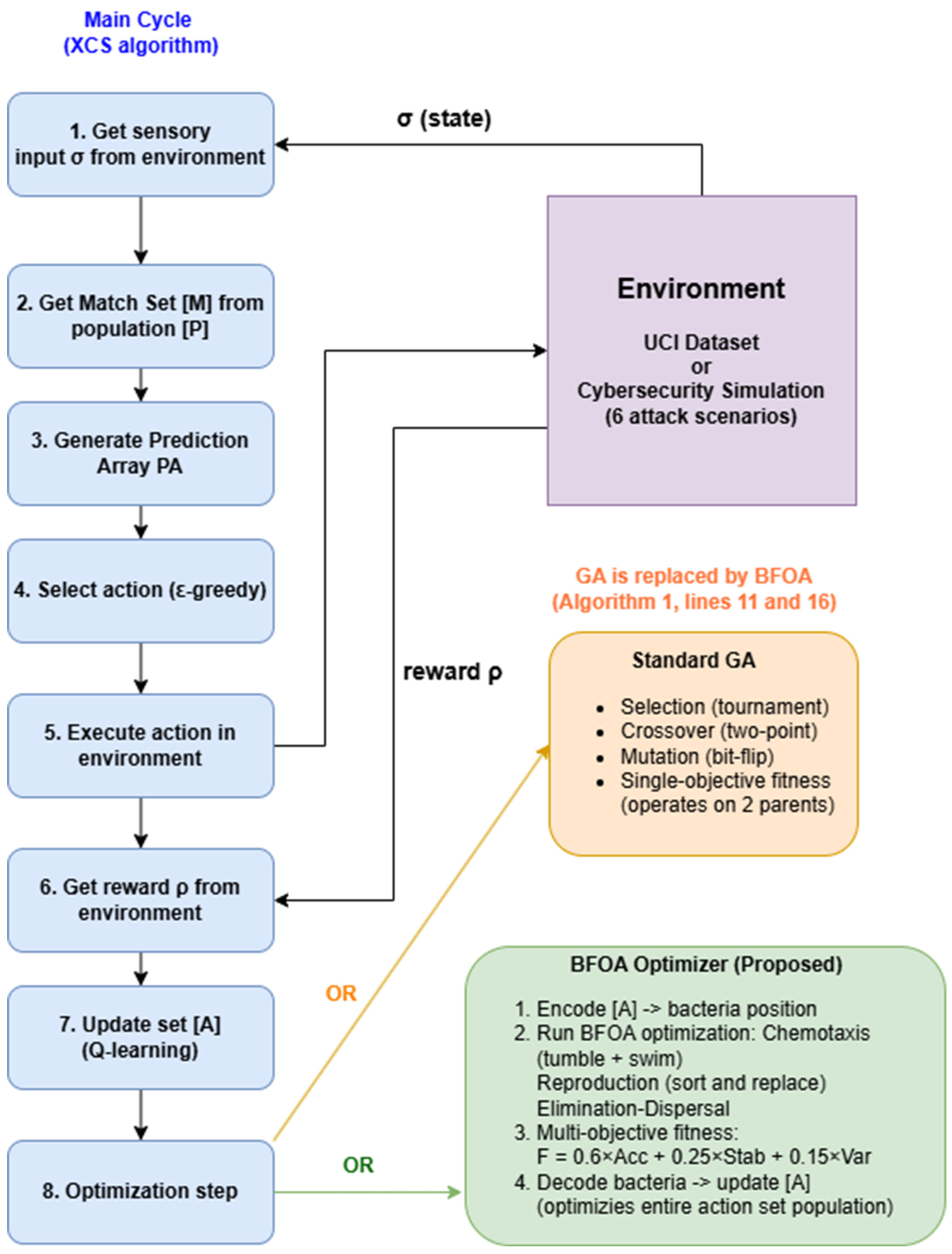
Figure 1 illustrates the integration architecture, showing the data flow between XCS’s action set and the BFOA optimizer.

3.3.1. Replacing GA with BFOA in XCS

In standard XCS, the GA is invoked at lines 11 and 16 of Algorithm 1, where it applies selection, crossover, and mutation operators to the classifiers in the current action set [A]. In the proposed BFOA-XCS system, this GA invocation is replaced with a call to the BFOA optimizer, while the remainder of the XCS cycle remains unchanged (that includes [M] formation, PA generation, action selection, and Q-learning parameter updates). The integration operates through a three-phase process: encoding, optimization, and decoding.
When BFOA is triggered, each classifier in the action set [A] is converted into a bacterium whose position is a real-valued vector in a continuous search space. The position vector has D = L + 1 dimensions, where L is the condition length of the classifier and the additional dimension represents the classifier’s action value. Condition bits are encoded as follows: a don’t-care symbol ‘#’ is mapped to 0.5, a bit value of 0 is mapped to 0.25, and a bit value of 1 is mapped to 0.75. The action value is normalized to [0, 1] using the minimum and maximum values of the target attribute from the dataset. All dimensions are thus bound within [0, 1], creating a uniform search space for BFOA’s chemotactic movement.
With the bacteria population initialized from the [A] classifiers, the selected BFOA variant (Standard, Adaptive, or IBFOA) executes its full optimization cycle as described in Section 3.2. Each bacterium is evaluated using the fitness function described in Section 3.3.2. The number of bacteria equals the number of classifiers in the [A], meaning that BFOA directly optimizes the existing classifier population rather than generating new individuals. This is a fundamental difference from the GA approach, where crossover produces new offspring. BFOA instead adjusts the existing classifiers’ parameters through continuous movement in the search space.
After optimization completes, the optimized bacterium positions are mapped back to the classifiers. In the current implementation, only the action values are updated from the optimized positions, while the classifier conditions are preserved. This constitutes a deliberate separation of concerns within the XCS learning cycle: BFOA serves as an action-parameter optimizer that refines what each classifier proposes, while XCS’s covering mechanism and condition matching logic retain full responsibility for structural exploration, that is, generating new rule conditions that match previously unseen states. This separation avoids the disruptive effects that continuous-valued perturbations would have on XCS’s binary condition representation, where small numerical changes to encoded condition bits could fundamentally alter which states a classifier matches. By contrast, the standard GA modifies both conditions and actions through crossover, which can disrupt well-fitted classifier conditions in mature populations. BFOA’s restriction on action-parameter optimization is therefore not a limitation but an architectural advantage: it enables fine-grained refinement of classifier actions without risking the structural integrity of the rule population. For classification tasks, the optimized continuous action value is snapped to the nearest valid class label to ensure consistency with the discrete action space. For regression tasks, the continuous value is applied directly.
Unlike the GA, which is triggered based on the average time stamp of classifiers in the action set (the θGA threshold), BFOA is invoked at a configurable frequency (i.e., every f iteration of the XCS main cycle). This design choice reflects the different computational profiles of the two approaches: the GA operates with lightweight crossover and mutation on two selected parents, whereas BFOA executes a full nested optimization loop (Ned × Nr × Nc chemotactic steps across all bacteria). Running BFOA at a reduced frequency (e.g., every 50 iterations) balances the computational cost while providing periodic population- level optimization that the GA’s operators at the individual level cannot achieve.
Algorithm 3 presents the pseudocode of the BFOA-XCS integration procedure, which replaces the GA calls at lines 11 and 16 of Algorithm 1.
Algorithm 3 Pseudocode of the BFOA integration into the XCS cycle (replaces GA at Algorithm 1, lines 11 and 16)
procedure RUN_BFOA(actionSet [A], sensory input σ)
    1. if [A] is empty then return
    2. N = number of classifiers in [A]
    3. D = condition length + 1
            // Map classifiers into a continuous-valued search space so BFOA’s
            // chemotactic movement can operate on the action set
    4. for each classifier cli in [A] do
    5.      for each condition bit j do
    6.          if cli.condition[j] = ‘#’ then pos[i][j] = 0.5
    7.          else if cli.condition[j] = 1 then pos[i][j] = 0.75
    8.          else pos[i][j] = 0.25
    9.      end for
  10.      pos[i][D] = normalize(cli.action, targetMin, targetMax)
  11. end for
        // Refine the action-set population through chemotaxis and
        // population dynamics under the multi-criteria fitness
  12. Select BFOA variant (Standard or Adaptive or IBFOA)
  13. Initialize optimizer with pos, bounds = [0, 1]D, fitness function F
  14. optimizedpos = optimizer.optimize()
        // Write optimized action values back to the classifiers. Conditions
        // are deliberately left unchanged to preserve XCS’s binary rule
        // representation and avoid disrupting mature populations.
  15. for each classifier cli in [A] do
  16.      actionraw = denormalize(optimizedpos[i][D], targetMin, targetMax)
  17.      if classification task then
  18.          cli.action = snapToNearestClass(actionraw)
  19.      else
  20.          cli.action = actionraw
  21.      end if
  22. end for
end procedure

3.3.2. Multi-Objective Classifier Fitness Function

A key advantage of integrating BFOA into XCS is the ability to evaluate classifier quality across multiple objectives simultaneously. In the standard GA-XCS, classifier fitness is derived solely from prediction accuracy. Classifier fitness is derived from prediction accuracy, which is computed from the classifier’s prediction error ε [58]. While effective, this single-objective approach does not account for the consistency or stability of classifier predictions over time. The proposed BFOA-XCS system introduces a multi-objective fitness function F that evaluates each bacterium (classifier) across three complementary objectives: prediction accuracy, prediction stability, and variance reduction.
The combined fitness is computed as a weighted sum:
F = wa × Saccuracy + ws × Sstability + wv × Svariance,
where wa = 0.60, ws = 0.25, and wv = 0.15 are the objective weights (Σw = 1), and the three score components Saccuracy, Sstability, and Svariance are defined below. This weighted-sum formulation constitutes a scalarized multi-criteria fitness rather than a Pareto-based multi-objective optimizer. The scalarized approach was chosen for computational efficiency, as evaluating a Pareto front within each BFOA chemotactic step would be prohibitively expensive for the inner-loop optimization setting. Since BFOA minimizes its objective function, the final cost passed to the optimizer is 1 − F, ensuring that higher-quality classifiers receive lower cost values.
Prediction Accuracy (Saccuracy) component measures how correctly a classifier’s action (predicted class or regression value) matches the expected output across the data instances to which the classifier’s condition applies. For classification tasks, accuracy is the fraction of correctly predicted instances. For regression tasks, it is derived from the normalized prediction error. The accuracy score is bounded in [0, 1], where 1.0 represents perfect prediction.
Prediction Stability (Sstability) component measures the consistency of a classifier’s predictions over a sliding window of recent evaluations. The fitness function maintains a Fitness Accumulator, a sliding window of size W (default W = 75) that records normalized prediction values. The stability score is computed as:
Sstability = 1 − min(1, σ2w/0.25),
where σ2w is the sample variance of the predictions within the window. A stability score of 1.0 indicates that the classifier consistently produces the same prediction, while a score near 0.0 indicates erratic behavior. Normalization constant 0.25 corresponds to the maximum possible variance for values bounded in [0, 1].
Variance Reduction (Svariance) component provides an additional penalty for prediction volatility using an Exponential Moving Average (EMA) of the variance. The EMA variance is updated incrementally:
Vema = (1 − α)·(Vema + α·δ2),
where α is the smoothing parameter (default α = 0.01) and δ = xt − μema is the deviation of the current prediction xt from the EMA mean μema. The variance score is then:
Svariance = 1 − min(1, Vema2),
where λ (default λ = 0.08) is a normalization parameter. The EMA-based variance provides a temporally smooth signal that responds gradually to changes, complementing the window-based stability score.
Accuracy alone can be misleading when a classifier achieves high accuracy sporadically but produces inconsistent predictions across different data presentations. The stability component rewards classifiers that produce consistent output, while the variance component penalizes long-term prediction drift. Together, these three objectives guide BFOA toward classifier populations that are not only accurate but also reliable. This multi-objective evaluation is made possible by BFOA’s population level optimization. Because BFOA evaluates all classifiers within [A] as a coordinated population of bacteria, it naturally supports simultaneous assessment across multiple fitness dimensions. By contrast, the standard GA evaluates individual classifiers in isolation, making multi-objective population level optimization less straightforward.
The weights wa = 0.60, ws = 0.25, wv = 0.15 were established through a two-stage preliminary empirical study conducted prior to the main experimental grid. In the first stage, a grid sensitivity check across eight weight triples (8 triples × 2 runs × 2000 iterations) confirmed that mean accuracies vary by only 0.0017 across the candidate range, establishing that the operator comparison is robust to weight choice within this range. In the second stage, a four-configuration ablation on the Breast Cancer dataset (4 configurations × 3 runs × 3000 iterations) compared an accuracy-only baseline (1.00, 0.00, 0.00), a +Stability configuration (0.75, 0.25, 0.00), the proposed (0.60, 0.25, 0.15) triple, and a high-stability variant (0.50, 0.35, 0.15). All four configurations produced statistically indistinguishable mean accuracies, but the (0.60, 0.25, 0.15) triple produced the lowest run-to-run standard deviation (a 17.1% reduction relative to the accuracy-only baseline), precisely the property the variance-reduction component is intended to deliver. The selection criterion was therefore: among configurations of equivalent mean accuracy, the triple producing the lowest run-to-run variance is selected. A supplementary replication across four datasets from the main experimental grid (Breast Cancer, Iris, Heart Disease, Wine Quality) further confirmed that the alternative weight triple used in earlier code versions (0.85, 0.10, 0.05) is empirically inferior, losing by 6.21% accuracy on Heart Disease relative to the proposed triple. Accuracy receives the dominant weight to ensure that prediction quality remains the primary optimization objective, consistent with XCS’s accuracy-based fitness philosophy. Stability receives a secondary weight to promote consistent classifier behavior, and variance reduction receives a tertiary weight as a smoothing regularizer. These weights were held constant across all experiments in this work.

3.4. Cybersecurity Simulation Environment

To evaluate BFOA-XCS in a dynamic, multi-step RL setting, a research cybersecurity simulation environment was designed, which will be presented in this subsection. The environment models a network under active attack, where a defending agent (i.e., algorithm in testing) must select protective actions at each time step to prevent the spread of threats across the network. This section describes the network topology, state representation, action space, attack dynamics, reward structure, and scenario profiles.

3.4.1. Network Topology

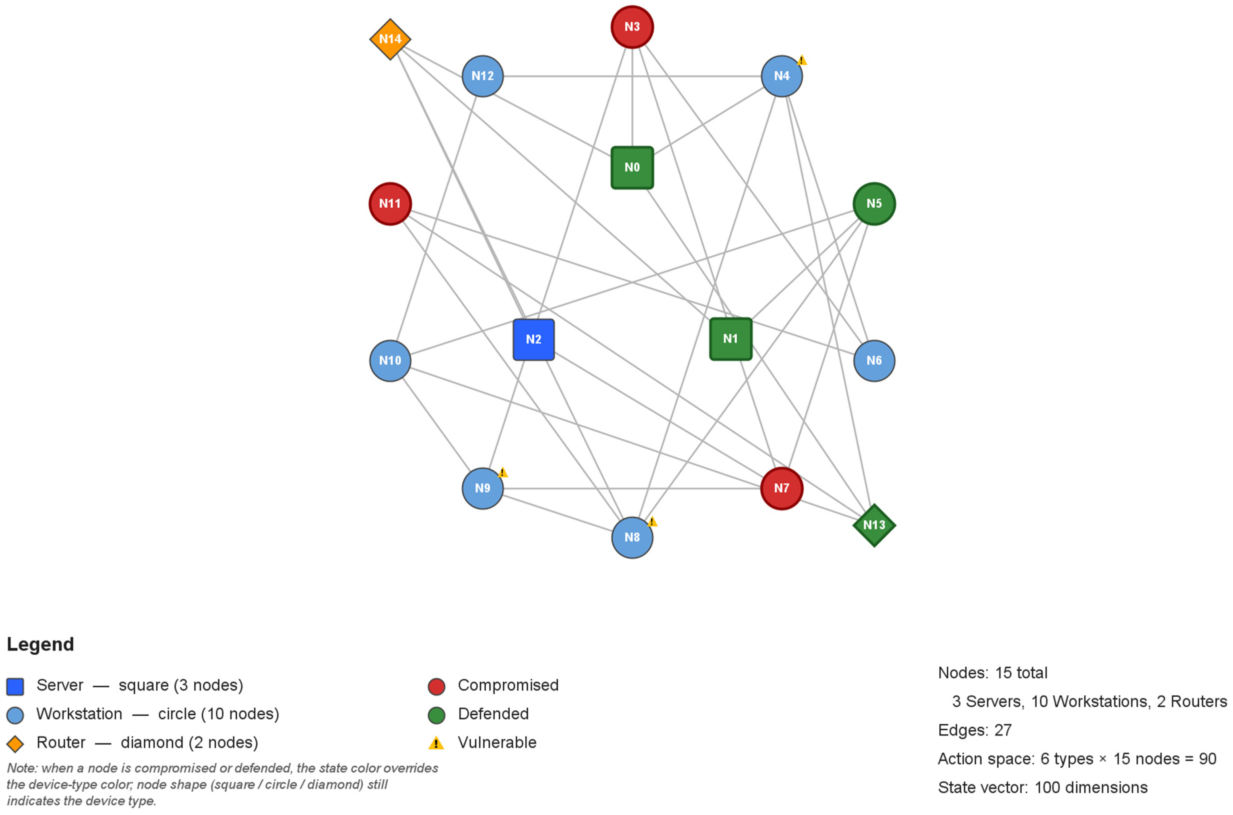
The simulated network consists of 15 nodes arranged in a medium-size topology comprising three servers, ten workstations, and two routers (Figure 2). Nodes are connected through network edges, forming a graph structure where attack propagation follows the adjacent relationships. Each node maintains three properties relevant to the defense task: a compromised flag (indicating active infection), a defended flag (indicating active protection), and a list of known vulnerabilities, which are visually indicated with yellow markers in the figure.

3.4.2. State Representation

At each time step, the environment state is encoded as a feature vector of fixed size of 100 dimensions. The first five features capture global network status: the fraction of compromised nodes, the fraction of defended nodes, the normalized time step, the fraction of vulnerable (undefended, uncompromised) nodes, and the normalized cumulative damage. The remaining features encode per-node information, with four features per node: compromise status (binary), defense status (binary), normalized vulnerability count, and normalized connection degree. All features are bounded in [0, 1]. Each continuous feature is converted into a 4-bit binary representation for XCS’s condition matching, where the [0, 1] range is partitioned into 16 equal intervals, and the feature value is encoded as the corresponding 4-bit binary code. This produces a total condition length of 400 bits (100 features × 4 bits) for each classifier.

3.4.3. Action Space

The defending agent selects from a discrete action space of 90 actions, composed of 6 action types applied to each of the 15 network nodes (6 × 15 = 90). The action types are:
  • Defend Node: Removes compromise and applies defense. Rewards correctly targeting compromised (+10) or vulnerable (+3) nodes and penalizes defending nodes that are already safe (−2 for safe, −1 for already defended).
  • Isolate Node: Disconnects a node from the network. Rewards isolating compromised nodes (+7), penalizes isolating clean nodes (−3).
  • Patch Node: Removes all vulnerabilities from a node and applies defense. Rewards patching vulnerable nodes (+5).
  • Monitor Node: Places surveillance on a node. Small reward for monitoring suspicious nodes (+1).
  • Restore Node: Reconnects a previously isolated node. Rewards restoring isolated nodes (+3).
  • Do Nothing: No action is taken. Receives a constant penalty (−2) to discourage passivity.
This large, structured action space (90 discrete actions) represents a key characteristic of the experimental setting and is a challenging environment for many agents (e.g., neural-network agents that rely on softmax action selection) but should show as a strength for XCS, which uses rules as its modus operandi, where each classifier directly maps a state condition to a specific action.

3.4.4. Attack Dynamics

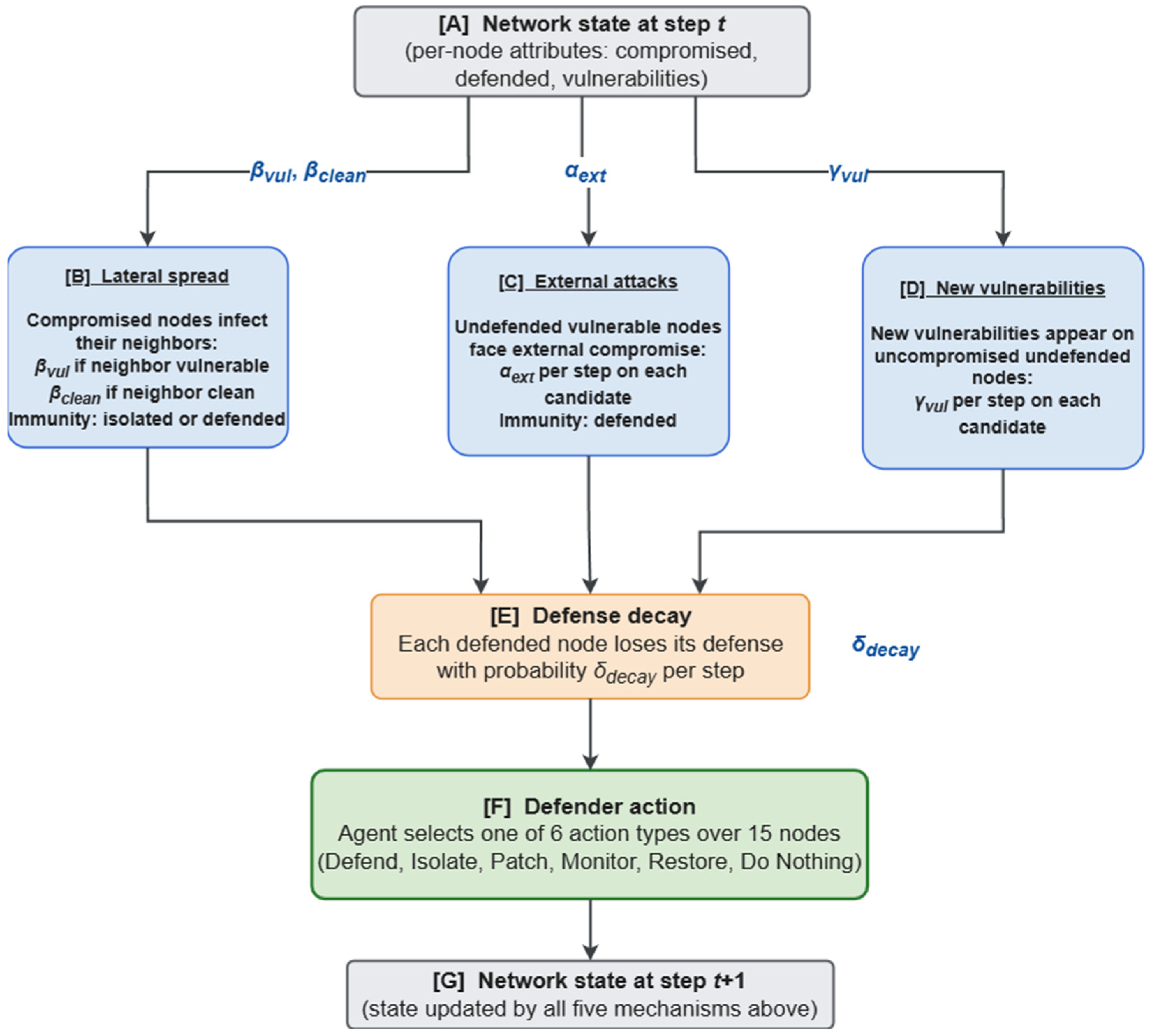
The environment simulates ongoing cyber-attacks through three concurrent threat vectors and a defense-decay mechanism that operate at each time step (Figure 3, Table 2). At every step t, the simulator updates the network state in a fixed order. First, lateral spread propagates compromise from infected nodes to their neighbors according to per-edge probabilities βvul if the neighbor is vulnerable or βclean if the neighbor is clean. Nodes that are isolated or currently defended are immune. Second, external attacks compromise undefended vulnerable nodes with probability αext per step, modeling pressure from outside the network. Third, new vulnerabilities emerge on uncompromised, undefended nodes with probability γvul per step, capturing the continuous discovery of latent software flaws. Finally, the defense-decay mechanism causes each defended node to lose its defensive posture with probability δdecay per step, reflecting the finite lifetime of patches, monitoring rules, and operator attention. Once all four mechanisms have been applied to the state at step t, the defender agent observes the resulting state and selects one of six action types (Defend, Isolate, Patch, Monitor, Restore, or Do Nothing), across the fifteen network nodes, producing the network state at step t + 1.
Parameter symbols (βvul, βclean, αext, γvul, δdecay) correspond to the per-step probabilities defined in Table 2, with scenario-specific values listed in Table 3.

3.4.5. Reward Structure

The reward function combines three components at each time step. First, an action reward provides immediate feedback based on the appropriateness of the selected action (as described in the previous subsection). Second, a state-change reward penalizes new node compromises (−8 per newly compromised node) and rewards successful remediation (+3 per cleaned node), with a constant time penalty (−0.3) to encourage efficient defense. Third, an episode termination reward is applied when the episode ends: a terminal penalty (−30) if the network reaches the compromise threshold or a survival bonus (up to +30, scaled by remaining network health) if the agent successfully maintains the network.
An episode terminates when either the fraction of compromised nodes exceeds the scenario-specific threshold (55–60%, depending on scenario) or the maximum step count (500) is reached.

3.4.6. Scenario Profiles

To evaluate agent adaptability across diverse threat landscapes, six distinct scenario profiles were designed, each with different attack rates, initial conditions, and dynamics. Table 3 summarizes the key parameters for each scenario.

4. Experimental Evaluation

This section presents the empirical evaluation of the proposed BFOA-XCS integration through two complementary experiments. Experiment 1 evaluates the BFOA-XCS variants on 19 benchmark datasets spanning classification, regression, and cybersecurity domains, establishing the general-purpose behavior of the proposed optimizer against the standard GA and a no-optimization baseline. Experiment 2 evaluates BFOA-XCS in a dynamic, multi-step cybersecurity defense setting against five deep reinforcement-learning baselines, demonstrating applicability beyond static supervised tasks. The two experiments share methodological choices (statistical validation, hyperparameter handling, hardware) but differ in task type, baselines, and evaluation metrics, motivating separate setup and results subsections within this unified evaluation chapter.

4.1. Experiment 1: Benchmark Machine Learning Datasets

The first experiment evaluates the BFOA-XCS integration on static classification and regression tasks using established benchmark datasets. The purpose is twofold: to verify that replacing the GA with BFOA does not degrade XCS’s operational capabilities and to assess whether BFOA’s multi-objective population optimization provides measurable improvements in prediction accuracy, stability, and variance reduction compared to the standard GA and the no-optimization baseline.

4.1.1. Experimental Setup

The experiment was conducted across 19 datasets spanning three categories: seven classification datasets, five regression datasets, and seven cybersecurity datasets (Table 4). The majority of classification and regression datasets originate from the UCI Machine Learning Repository, supplemented by additional domain-specific datasets (Neurofibromatosis, Paddy Yield). The classification datasets range from well-known benchmarks (Iris, Breast Cancer, Wine) to more challenging problems (Ionosphere, Neurofibromatosis). The regression datasets cover diverse prediction tasks including housing prices, material strength, and wine quality. Regression targets were discretized into 41 equal-width bins, transforming the original regression task into an ordinal classification problem. This approach was chosen because XCS’s rule-based action matching and action set formation require discrete action labels. While bin-based accuracy does not capture ordinal proximity (e.g., a prediction one bin away is penalized the same as one twenty bins away), it provides a consistent evaluation metric across all dataset types in our experimental grid.
The primary purpose of the regression datasets in this study is comparative (i.e., evaluating relative operator performance rather than absolute regression quality), which mitigates this limitation. The cybersecurity datasets include two industry standard intrusion detection benchmarks (NSL-KDD (Network Security Laboratory–KDD; revised KDD Cup 1999 intrusion detection benchmark dataset) and UNSW-NB15 (University of New South Wales Network-Based 2015 intrusion detection dataset)), using 20% stratified random subsets to maintain computational feasibility across the experimental grid, evaluated in both binary and multiclass settings, one additional intrusion detection benchmark (KDD Test+), and a ransomware dataset evaluated with two different targets (binary detection and family classification).
For all datasets, numeric features (excluding the target column) were normalized using min–max scaling, with the minimum and maximum values computed from the training split and propagated to the test and validation splits to prevent information leakage. The target column was excluded from the state representation during encoding. Categorical features were encoded using binary encoding with dataset-specific category maps. For the Ransomware dataset, per-dataset column exclusions were applied to prevent target leakage: the ‘family’ column was excluded when predicting ‘RG’, and the ‘RG’ column was excluded when predicting ‘family’. Additionally, identifier columns (e.g., IDs, filenames, timestamps) were excluded globally across all datasets. Missing values in the Neurofibromatosis dataset (~13% of instances) were handled through the encoder’s don’t-care mechanism, which maps missing values to generalized classifier conditions.
Five XCS operator configurations were compared: NONE (no optimization: XCS runs without any evolutionary or swarm-based operator), GA (standard genetic algorithm), BFOA, Adaptive BFOA, and IBFOA. Each configuration was evaluated across four P# (don’t-care probability) values: 0.33, 0.50, 0.60, and 0.70. Each configuration was executed 10 times with different random seeds. Classification and cybersecurity datasets were evaluated at both 5000 and 10,000 training iterations, while regression datasets used 5000 iterations. This yielded a total of 5600 experiments (19 datasets × 5 operators × varying configurations × 10 runs).
All datasets were split using stratified sampling with a 70/20/10 train/test/validation ratio. XCS was configured with a population size of 500 classifiers, exploration rate of 0.10, crossover probability of 0.80, mutation probability of 0.04, GA threshold θGA = 25, and subsumption threshold of 20 with both action set and GA subsumption enabled. The holdout test set (20%) was used for all reported accuracy values.
BFOA parameters were configured as follows: invocation frequency every 100 iterations, step size C = 0.02, chemotactic steps Nc = 25, reproduction steps Nr = 3, elimination-dispersal steps Ned = 1, swim length Ns = 4, bacteria population capped at 64, swarming disabled, and a warmup period of 20% of total iterations (during which BFOA is not invoked, allowing XCS to build an initial classifier population). The multi-objective fitness function was enabled with weights wa = 0.60, ws = 0.25, and wv = 0.15 as described in Section 3.3.2. An additional ablation run with multi-objective fitness disabled, which is an accuracy-only evaluation, was performed under otherwise identical conditions to isolate the contribution of the multi-objective fitness function.
Statistical validation followed the methodology recommended by Demšar [67] for comparing multiple classifiers across multiple datasets: the Friedman test for global ranking with the Iman–Davenport adjustment and the Wilcoxon signed-rank test for targeted pairwise comparisons. Effect sizes were quantified using Cohen’s d [68]. Variance reduction was computed as the percentage decrease in prediction standard deviation relative to the GA baseline. The Friedman test significance level was set to α = 0.10 a priori, consistent with the exploratory nature of this study: the primary goal is to identify whether BFOA optimization variants warrant further investigation as GA replacements, rather than to confirm a pre-registered hypothesis at the more conservative α = 0.05 level. Operator comparisons in this experiment rely on convergent evidence across multiple indicators (Friedman ranking, pairwise Wilcoxon, effect sizes, and an ablation study) rather than on any single test.
All experiments were conducted on a desktop PC equipped with an Intel Core i7-9700 processor and 32 GB of RAM, running Windows 11 Pro. The software environment consisted of OpenJDK 22, with IntelliJ IDEA 2025.3.1 (Community Edition) used as the development environment.

4.1.2. Results and Analysis

This section presents the results of the benchmark experiment, organized into four parts: the overall operator ranking, per-dataset accuracy analysis, variance reduction analysis, and an ablation study of the multi-objective fitness function.
Overall Operator Ranking
Table 5 presents the Friedman test results for all five operators across the 19 datasets. The Friedman test yielded χ2 = 8.895 with p = 0.064, marginally significant at the a priori α = 0.10 level (justified in Section 4.1.1). The Iman–Davenport corrected statistic was F = 2.386 with p = 0.059. The consistent ranking pattern and the supporting effect-size analysis (discussed below) provide convergent evidence of operator differences.
The key finding is that IBFOA achieves the best Friedman ranking, while the standard GA ranks fourth out of five operators. All three BFOA variants (BFOA, Adaptive BFOA, and IBFOA) together hold ranks 1, 3, and 5, with IBFOA and standard BFOA both outranking the GA. The NONE baseline ranks second, which indicates that the standard GA optimization in XCS does not consistently improve upon the unoptimized baseline across diverse datasets, a finding that supports the motivation for exploring alternative optimization approaches.
Per-Dataset Accuracy
The per-dataset accuracies in Table 6 are presented under oracle configuration selection: for each operator–dataset pair, the (P#, iteration count) configuration that produced the highest mean accuracy over 10 runs is selected post hoc, and the corresponding holdout accuracy is reported. Table 6 therefore presents upper-bound per-operator performance for illustrative comparison only and is not the basis for the statistical claims of this paper. The statistical analyses elsewhere in Section 4.1.2 (Friedman rankings, effect sizes, and variance reduction) are computed across all configurations without post hoc selection, ensuring that the evidential claims are not affected by configuration-level optimistic bias.
In terms of dataset wins (highest accuracy per dataset), NONE achieved the best accuracy on 10 of 19 datasets, GA on 6, BFOA on 6, Adaptive BFOA on 5, and IBFOA on 5 (ties counted for every operator that achieves the best value). Two patterns underlie these counts. First, on the three regression datasets (Auto MPG, Concrete Strength, Paddy Yield), all operators converge to nearly identical accuracies and therefore tie, contributing equally to every operator’s total. Second, NONE’s lead in unique wins (i.e., outright best, not shared) comes from several cybersecurity datasets (KDD Test+, Ransomware RG, UNSW-NB15 Multi) and a few classification datasets (Iris, Wine), where the unoptimized baseline outperforms every evolutionary and swarm-based operator. This pattern suggests that, on datasets where XCS’s native learning mechanisms already find near-optimal rules, adding optimization provides minimal benefit.
However, where optimization does make a difference, BFOA variants outperform the GA. On Breast Cancer, IBFOA achieves the highest accuracy (0.772 vs. GA’s 0.758). On Wine Quality, IBFOA (0.539) substantially outperforms GA (0.433). On NSL-KDD Multiclass, standard BFOA (0.394) outperforms both GA (0.368) and NONE (0.365). On Neurofibromatosis, BFOA (0.566) achieves the best result, where GA (0.544) underperforms even the baseline.
Effect Sizes and Pairwise Comparisons
While the Wilcoxon signed-rank tests comparing each operator against GA did not yield individually significant p-values (p = 0.220–1.000), the Cohen’s d effect sizes reveal consistent and meaningful differences in favor of all operators over GA (Table 7).
All four comparisons show medium-to-large effect sizes favoring the alternative operator over GA. The largest effect size is observed for NONE vs. GA (d = 0.803), suggesting that the standard GA may, in some cases, disrupt otherwise functional classifier populations through its crossover and mutation operations. Among the BFOA variants, IBFOA shows the strongest effect (d = 0.737), followed by BFOA (d = 0.693) and Adaptive BFOA (d = 0.623). Importantly, these effect sizes are computed across all 19 datasets using the best configuration per dataset, reflecting a robust comparison that is not sensitive to individual dataset selection.
Variance Reduction
A central claim of the multi-objective fitness function (Section 3.3.2) is that it simultaneously optimizes accuracy, stability, and variance reduction. Table 8 presents the variance reduction achieved by each operator relative to GA.
IBFOA achieves the most substantial variance reduction at 15.2% relative to GA, meaning that IBFOA’s predictions are considerably more consistent across datasets and runs. All operators show positive variance reduction relative to GA, indicating that the GA’s stochastic crossover and mutation operators introduce prediction instability that the alternatives avoid.
Multi-Objective Fitness Ablation
To isolate the contribution of the multi-objective fitness function, a complete ablation experiment was conducted under identical conditions with the multi-objective fitness disabled (accuracy-only evaluation). Table 9 compares the key metrics between both conditions.
The ablation reveals three important findings. First, the multi-objective fitness function produces a substantially stronger statistical signal, with the Friedman p-value improving from 0.185 (not significant) to 0.064 (marginally significant). Second, with multi-objective fitness enabled, IBFOA is promoted from second to first in the Friedman ranking, while without it, the unoptimized baseline (NONE) ranks first, indicating that the accuracy-only fitness landscape is too flat for the metaheuristic optimizers to provide meaningful differentiation. Third, and most critically, the multi-objective fitness function delivers consistent variance reduction across all operators, whereas under accuracy-only evaluation, three of four operators (NONE, BFOA, Adaptive BFOA) exhibit increased variance relative to GA. This confirms that the stability and variance components of the fitness function (Equations (2)–(4) in Section 3.3.2) are operating as intended, rewarding stable classifier populations and penalizing erratic prediction behavior.
Summary of Key Findings
The first experiment establishes four key results. First, replacing GA with BFOA does not degrade XCS’s performance. IBFOA achieves the top Friedman ranking across 19 datasets (p = 0.064, marginally significant at α = 0.10), while GA consistently ranks fourth. Second, the multi-objective fitness function substantially enhances the effectiveness of BFOA-based optimization, improving the Friedman p-value from 0.185 to 0.064 and producing consistent variance reduction. Third, the effect sizes confirm that all operators outperform GA with medium-to-large effects (Cohen’s d = 0.623–0.803), demonstrating that the GA component is the weakest optimization choice for XCS across diverse problem domains. Fourth, IBFOA emerges as the strongest variant, combining the best Friedman rank with the largest variance reduction (15.2%), validating the combination of Lévy flights and global elitism for classifier population optimization.

4.2. Experiment 2: Dynamic Cybersecurity Defense

The second experiment evaluates BFOA-XCS in a fundamentally different setting: a dynamic, multi-step cybersecurity simulation where an intelligent defender must make sequential decisions against ongoing attack scenarios. Unlike the static classification and regression tasks of Experiment 1, this environment requires each agent to learn a defensive policy through online interaction with a simulated network under six distinct attack profiles. The experiment compares the twenty XCS agent configurations against six DRL baselines, providing insight into how rule-based and neural approaches perform in structured, high-dimensional discrete action spaces.

4.2.1. Experimental Setup

The experiment uses the cybersecurity simulation environment described in Section 3.4, with the six scenario profiles defined in Table 2: DDoS flooding, network intrusion, ransomware propagation, port scanning reconnaissance, data exfiltration, and a mixed-attack scenario that combines elements of all five. The network topology consists of 15 nodes (three servers, ten workstations, two routers), resulting in a state vector of 100 continuous dimensions (five global features: fraction of compromised nodes, fraction of defended nodes, normalized time step, fraction of vulnerable nodes, and normalized cumulative damage; plus four per-node features for each node: compromise status, defense status, normalized vulnerability count, and normalized connection degree) and a discrete action space of 90 actions (six defensive action types, Defend Node, Isolate Node, Patch Node, Monitor Node, Restore Node, and Do Nothing, applied to each of the 15 nodes).
The simulation environment is intended as a controlled abstraction that captures the dynamics most directly relevant to closed-loop defensive policy learning rather than as a faithful replica of an enterprise network. Aspects such as encrypted traffic, heterogeneous device configurations, partial observability beyond the modeled state vector, and adversarial co-adaptation are not modeled (see Section 5.2).
Twenty XCS agent configurations were tested: five operators (NONE, GA, BFOA, Adaptive BFOA, IBFOA) crossed with four P# values (0.33, 0.50, 0.60, 0.70). Each XCS agent was configured with a population of 500 classifiers, 4 bits per feature (producing 400-bit conditions), and an exploration rate decaying from 0.10 to 0.01 (decay factor 0.995 per episode). BFOA parameters were adjusted relative to Experiment 1 to suit the dynamic environment: the invocation frequency was set to every 50 episodes (resulting in twenty BFOA optimizations per 1000-episode run, compared to every 100 iterations in Experiment 1), and the inner loop budget was increased to Nc = 50, Nr = 4, Ned = 2 (compared to Nc = 25, Nr = 3, Ned = 1 in Experiment 1). These changes double the optimization cadence and increase the per-trigger computational effort, providing more thorough population refinement in the dynamic setting. The multi-objective fitness function was enabled with the same weights as Experiment 1 (wa = 0.60, ws = 0.25, wv = 0.15).
Six DRL baselines were included for comparison. All neural agents were implemented from scratch in Java with manual backpropagation, as no production-ready pure Java implementations of PPO or SAC exist, to the best of the authors’ knowledge. Existing open-source PPO/SAC implementations (e.g., RLlib, version 2.55.1, part of the Ray framework) are available only in Python/C++. Implementation correctness was verified through a diagnostic test suite covering reward normalization stability, loss convergence, and action distribution analysis across multiple reward scales, with both PPO and SAC passing all eight diagnostic tests.
The baseline configurations used in the experiment were:
  • DQN (Deep Q-Network): learning rate 0.001, discount factor γ = 0.99, ε-greedy exploration with ε = 0.1.
  • Q-Learning: tabular with learning rate 0.1, γ = 0.95, ε = 0.1, and state discretization into 10 bins.
  • Policy Gradient (REINFORCE): the foundational policy gradient algorithm [69], learning rate 0.001, γ = 0.95.
  • PPO (Proximal Policy Optimization): learning rate 0.001, γ = 0.99, clip ε = 0.2, GAE-λ (Generalized Advantage Estimation) = 0.95, 4 epochs per update. For PPO, the clip-region check in the surrogate objective uses a non-strict comparison: the unclipped policy gradient is applied whenever surr1 ≤ surr2, ensuring that the gradient flows when the importance ratio lies inside the clip interval [1 − ε, 1 + ε], including at its boundary. This is consistent with the surrogate objective specified by Schulman et al. (2017) [70].
  • SAC (Soft Actor–Critic, discrete variant): actor learning rate 0.00015, critic learning rate 0.0003, γ = 0.99, initial entropy coefficient α = 0.2 with automatic tuning, target entropy ratio 0.5, Polyak τ = 0.005, replay buffer capacity 10,000, batch size 64, warmup 128 steps.
  • Random: uniformly random action selection (lower-bound baseline).
All neural baseline agents use feedforward architectures with Leaky ReLU activations (α = 0.01) in hidden layers and linear output layers. DQN uses a single network with architecture [100, 100, 50, 90] (input, two hidden layers, output). Policy Gradient uses the same architecture for its policy network. PPO uses separate actor [100, 100, 50, 90] and critic [100, 100, 50, 1] networks. SAC uses larger networks due to its five-network architecture: actor [100, 200, 100, 90] and four critic networks (two online, two target) each [100, 200, 100, 90]. All networks use He initialization and element-wise gradient clipping (clip value 1.0). Input normalization (Welford’s online algorithm for running mean and variance) and reward normalization (Welford’s with clip to ±10) are applied in DQN, PPO, and SAC. DRL hyperparameters were set to standard values from the original publications without environment-specific tuning, consistent with the XCS configurations that also used fixed hyperparameters across all scenarios.
Each of the 26 agent configurations (twenty XCS and six baselines) was run ten times per scenario with fixed random seeds (base seed 42), resulting in 1560 total runs (26 × 6 × 10). Each run consisted of 1000 training episodes with a maximum of 300 steps per episode. The primary performance metric is the mean cumulative reward across all episodes, which reflects the agent’s overall policy quality including the learning trajectory. The total experiment runtime was approximately 18 h 49 min. Statistical validation employed the same methodology as Experiment 1: the Friedman test with Iman–Davenport correction for global ranking, the Nemenyi post hoc test for multiple comparisons, the Wilcoxon signed-rank test for targeted pairwise comparisons, and Cohen’s d for effect size quantification. The Wilcoxon test uses 60 per-run paired observations (six scenarios × ten runs) to ensure sufficient statistical power.

4.2.2. Results and Analysis

This section presents the results of the cybersecurity defense experiment, organized into three parts: overall agent ranking, per-scenario analysis, and the sensitivity to P# (don’t-care probability) configuration.
Overall Agent Ranking
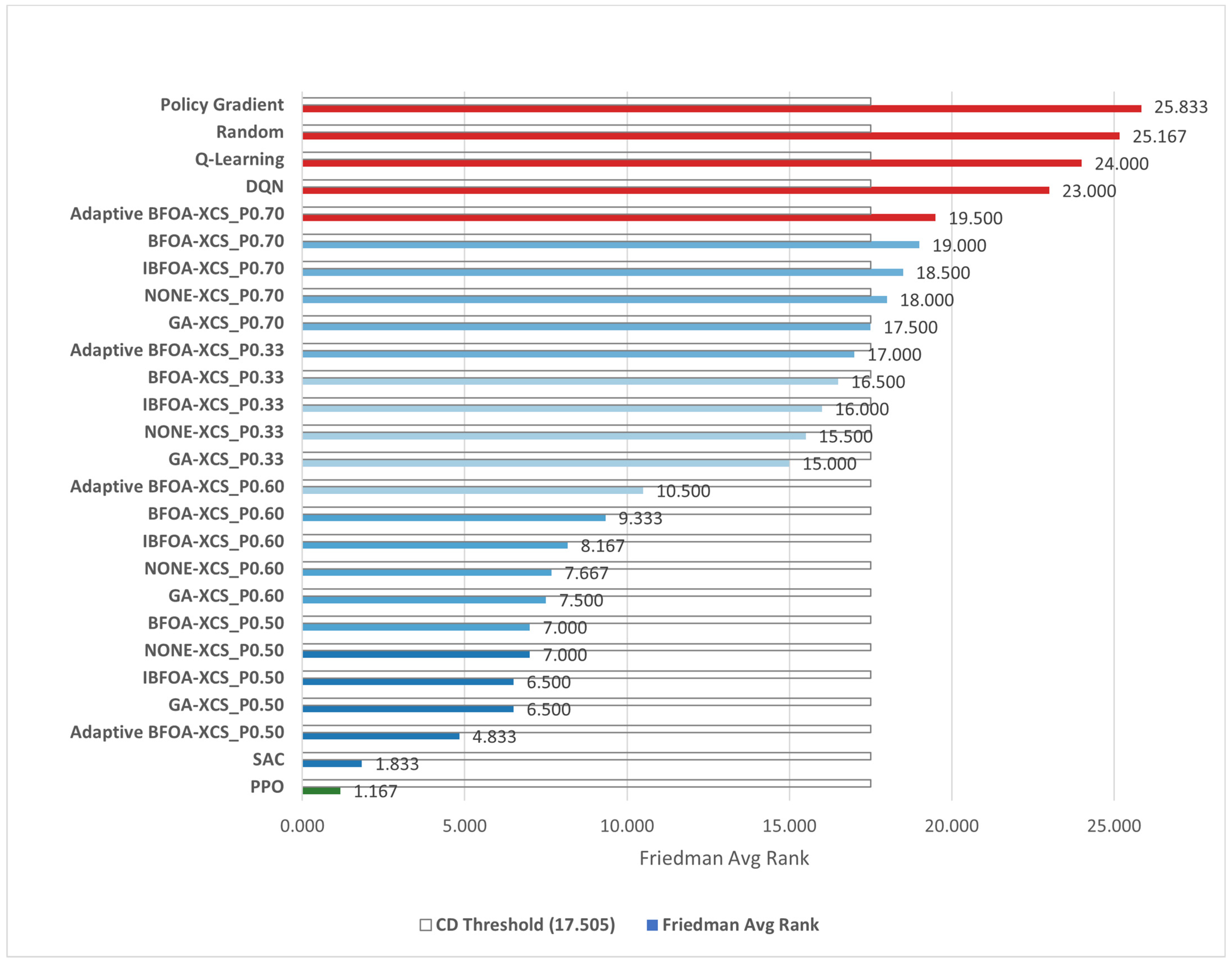
Table 10 presents the overall ranking of all 26 agent configurations by mean cumulative reward, alongside the Friedman test rankings across the six scenarios. The Friedman test yielded χ2 = 136.45 with p ≈ 0 (Iman–Davenport F = 50.35, p ≈ 0), confirming highly significant differences among agents.
PPO achieves the highest overall performance, with a mean reward of +307.57 and the best Friedman rank (1.167), followed by SAC (mean +110.65, rank 1.833). All XCS variants at P# = 0.50 achieve positive mean rewards (+5.82 to +6.60) and occupy Friedman ranks 4.833 to 7.000, forming a third tier. Among the XCS configurations, Adaptive BFOA-XCS at P# = 0.50 achieves the best Friedman rank (4.833), followed by GA-XCS (6.500), IBFOA-XCS (6.500), NONE-XCS (7.000), and BFOA-XCS (7.000). DQN is the best-performing of the remaining DRL baselines (rank 23.000, mean −28.34) but scores 34 points below the weakest XCS P# = 0.50 variant. Q-Learning (rank 24.000, mean −47.98), Random (rank 25.167, mean −80.12), and Policy Gradient (rank 25.833, mean −86.12) occupy the bottom of the ranking. The Friedman ranking visualization is presented in Figure 4.
Per-Scenario Analysis
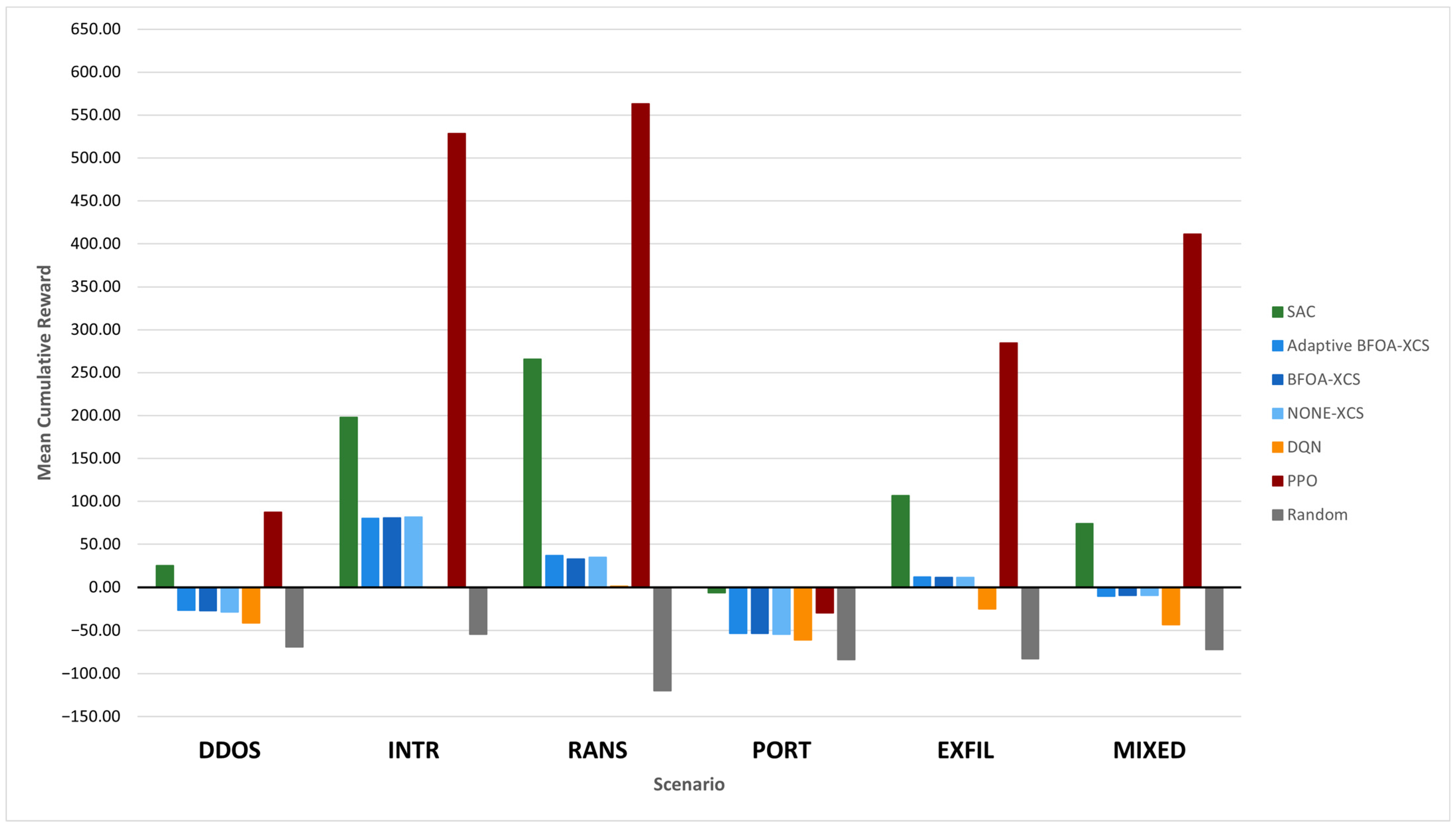
Table 11 presents the mean reward for selected agents across all six scenarios. Figure 5 provides the corresponding visual comparison.
Three performance tiers emerge consistently across the scenarios. The first tier consists of PPO and SAC, which achieve the highest rewards across most scenarios. PPO leads in four of the six scenarios (Intrusion +528.36, Ransomware +563.30, Data Exfiltration +284.72, Mixed +411.33), with SAC leading on DDoS (+25.41) and Port Scan (−6.11). Both top neural agents exhibit particularly strong performance on the most learnable scenarios, such as Ransomware and Intrusion. The second tier comprises all XCS variants at P# = 0.50, which achieve positive rewards on three of six scenarios (Intrusion, Ransomware, and Data Exfiltration) and moderately negative rewards on the others. The third tier contains DQN, Q-Learning, Random, and Policy Gradient, which achieve negative rewards across nearly all scenarios, with mean overall rewards in the −28 to −86 range.
Within the XCS tier, the per-scenario differences between operators are small. On Intrusion, NONE-XCS (+81.85) slightly outperforms BFOA-XCS (+80.85) and Adaptive BFOA-XCS (+80.20), suggesting that, for high-signal scenarios, XCS’s native learning mechanisms suffice. On Ransomware, Adaptive BFOA (+37.09) outperforms all other XCS operators, while on Data Exfiltration, Adaptive BFOA (+12.12) also leads. The most challenging scenario for all agents is Port Scan, where even SAC achieves only −6.11. The stealthy, low-signal nature of reconnaissance attacks makes defensive decision-making inherently difficult.
P# Sensitivity
The don’t-care probability (P#) has a strong and consistent effect on performance across all XCS operators. P# = 0.50 produces the best results (mean +5.82 to +6.60), followed by P# = 0.60 (+2.52 to +3.78). Both P# = 0.33 and P# = 0.70 yield negative mean rewards. At P# = 0.33, classifiers are too specific, producing narrow rules that fail to generalize across the diverse states encountered in the simulation. At P# = 0.70, classifiers are too general, producing overly broad rules that cannot discriminate between meaningful state differences. The optimal range of P# = 0.50–0.60 produces classifiers with balanced generality. That is specific enough to capture decision-relevant state features while general enough to transfer across related states within each scenario.
Classifier Population Analysis
To address scalability and population complexity associated with the 400-bit condition representation used in Experiment 2, three per-run classifier-population diagnostics were extracted from the cybersecurity-simulation logs at P# = 0.50 (the configuration that produced the best results), aggregated across the 30 (operator, scenario) cells: the final classifier population size [P], the mean condition specificity (the fraction of non-don’t-care bits per classifier), and the mean match-set size [M] in the steady-state (final 100) episodes of each run. The full per-cell results are reported in Table 12. The summary findings follow.
First, the average final classifier population size was 500 with zero variation across cells. XCS’s deletion-pressure mechanism reaches and holds the configured cap of 500 in every run, confirming that the 400-bit condition representation does not cause population growth beyond the design budget. Second, the average condition specificity was 0.5 (with a maximum cross-cell deviation of 0.0001), indicating that, on average, approximately 200 of the 400 bits per classifier condition are informative while the remainder are don’t-care wildcards, precisely the value expected at P# = 0.50 under uniform covering, confirming that the representation is not pathologically sparse and that no optimization operator drifts it from the design point. Third, the average [M] size in the steady-state episodes was 35.45 classifiers (i.e., approximately 7.1% of the population matches a typical state, with cell-level means ranging from 29.5 (Ransomware) to 40.7 (Port Scan)). This is well above the percent-level threshold below which sparse-match collapse would be a concern, and the moderate cross-scenario spread reflects the differing state-distribution diversity of the scenarios rather than any structural pathology.
The three metrics are statistically indistinguishable across the five optimization operators (per-operator means differ by at most 0.5 classifiers in [M] size and at most 0.0001 in specificity, both well below within-cell noise). This operator-agnostic structure is consistent with the separation-of-concerns architecture described in Section 3.3.1: because BFOA optimization refines classifier actions rather than conditions, the population-level structural statistics are determined by XCS’s covering and matching mechanisms and not by the choice of optimization operator. Together, these three diagnostics directly imply the following: the population is bounded, the conditions are not degenerate, and the [M] is dense enough for meaningful action selection.

4.2.3. Comparison with Deep Reinforcement Learning Baselines

This section analyzes the performance differences between XCS and the DRL baselines, addressing three aspects: statistical significance, the architectural factors underlying each agent’s performance, and the computational cost trade-off.
Statistical Significance
Table 13 presents the Wilcoxon signed-rank tests and Cohen’s d effect sizes for key pairwise comparisons against BFOA-XCS_P0.50 (the representative XCS variant).
BFOA-XCS significantly outperforms three of five DRL baselines (DQN, Q-Learning, Policy Gradient), with medium-to-large effect sizes (d = 0.776–2.873), and also significantly outperforms the Random baseline (d = 2.513). Both PPO and SAC significantly outperform BFOA-XCS in pairwise comparison (PPO: Wilcoxon p < 0.001, d = 1.179; SAC: Wilcoxon p < 0.001, d = 1.000), with large effect sizes in both cases. The Nemenyi post hoc test (critical difference CD = 17.505 at α = 0.01) confirms that XCS variants significantly outperform the bottom-tier DRL baselines (DQN, Q-Learning, Random, Policy Gradient) and that PPO and SAC significantly outperform the same DRL baselines. Notably, however, neither PPO nor SAC significantly outperforms any XCS variant at P# ∈ {0.50, 0.60} under Nemenyi correction (maximum rank difference 9.333 for PPO and 8.667 for SAC, both well below CD = 17.505), meaning that, while PPO and SAC clearly lead in pairwise Wilcoxon comparison, the advantage over XCS does not survive the conservative multiple-comparison correction. Within the top tier of agents (PPO, SAC, and XCS variants at P# ∈ {0.50, 0.60}), no pair is statistically distinguishable at α = 0.01 under Nemenyi.
Within the XCS family, pairwise Wilcoxon tests show no significant differences between operators (p = 0.220–0.868, d = 0.005–0.014), indicating that the choice of optimization operator has a negligible impact on overall performance in the dynamic environment. This contrasts with Experiment 1, where IBFOA achieved a meaningfully better Friedman rank and variance reduction, suggesting that the dynamic environment’s stochasticity dominates any operator-level differences.
Architectural Analysis
The performance hierarchy observed in this experiment reflects fundamental architectural differences between the agent types.
SAC achieves the second-highest performance (mean +110.65) due to three key architectural advantages for this environment. First, as an off-policy algorithm, SAC reuses past experiences via a replay buffer, allowing it to learn from each transition multiple times. That is a critical advantage given the 300,000-step training budget (1000 episodes × 300 steps). Second, SAC’s entropy regularization explicitly encourages exploration of the 90-action space, preventing premature convergence to suboptimal defensive strategies. Third, SAC’s twin Q-networks and automatic temperature tuning provide stable value estimation in the presence of the environment’s inherent stochasticity. Research on discrete SAC has noted that these advantages come with known trade-offs: Q-value underestimation and performance instability can emerge in discrete settings, and the computational overhead of maintaining five neural networks (actor, two critics, two target critics) plus a replay buffer is substantial.
XCS variants form a consistent second tier, achieving positive mean rewards despite a fundamentally different approach. XCS operates through a population of interpretable IF–THEN rules, each matching a subset of states and proposing defensive actions. This rule-based architecture provides three practical advantages. First, XCS exhibits warmup-free competence: the covering mechanism generates reasonable rules from the first episode, producing positive-reward behavior without a warmup period or replay buffer. In contrast, SAC requires 128 warmup steps before training begins. Second, XCS decisions are inherently interpretable. The matching rules can be inspected to understand why a particular defensive action was selected. Third, XCS’s computational footprint is substantially lower, as discussed under Computational Cost in Section 4.2.
DQN occupies a middle ground (mean −28.34), showing that a simpler off-policy architecture with a replay buffer can learn basic defensive patterns but lacks SAC’s entropy-driven exploration needed to navigate the 90-action space effectively. DQN’s ε-greedy exploration (ε = 0.1) provides only a 10% chance of random action selection, which is insufficient for discovering non-obvious defensive strategies across 90 actions.
PPO achieves the highest mean reward in this experiment (+307.57) after the implementation correction described next. The original PPO implementation contained a strict-inequality at the PPO-Clip branch selector (“if (surr1 < surr2)”) that zeroed the policy gradient throughout the unclipped region of the importance ratio, where surr1 equals surr2 bitwise within the [1 − ε, 1 + ε] interval. The canonical PPO-Clip surrogate objective of Schulman et al. (2017) [70] requires the unclipped policy gradient to flow at the equality boundary, which we ensure via non-strict comparison (“if (surr1 ≤ surr2)”). With this implementation, PPO’s clipping and GAE advantage estimation provide stable on-policy updates in the 90-action discrete cybersecurity environment, producing per-scenario means from +87.45 (DDoS) to +563.30 (Ransomware). Policy Gradient, in contrast, performs worse than the Random baseline (mean −86.12 vs. −80.12). As an on-policy algorithm without a clipping or trust-region mechanism, Policy Gradient discards collected experience after each gradient update and applies the raw policy gradient with no bound on policy drift between updates; in an environment with 90 discrete actions and only 1000 training episodes, this combination of sample inefficiency and unbounded update magnitudes prevents the policy from reaching a viable working point within the training budget. The contrast between PPO and Policy Gradient highlights that the clipping mechanism, and not the on-policy framing alone, determines whether a policy-gradient method can navigate a large discrete action space within a limited training budget.
Q-Learning (mean −47.98) fails because tabular Q-learning with state discretization into 10 bins cannot represent the 100-dimensional continuous state space with sufficient resolution, resulting in severe state aliasing where perceptually different network conditions map to the same discretized state.
Computational Cost
Table 14 presents the average computation time per run for each agent type, alongside the overall mean reward. Figure 6 illustrates the cost–performance trade-off.
PPO and SAC, the two top-performing agents, both come at substantial computational cost compared to XCS: PPO at an average 5.3× the XCS compute time per run (2 min 8 s vs. 24 s) and SAC at 26.1× (10 min 26 s vs. 24 s). PPO’s per-run cost reflects that the corrected agent successfully defends the network across most of the 300 steps of each episode in most scenarios, increasing the total number of environment–agent interactions per run. Agents that fail quickly terminate episodes early and therefore incur lower wall-clock cost per run despite their poor performance. SAC’s cost ratio varies by scenario, ranging from 15.8× on Ransomware (where SAC’s longer episodes involve more complex state transitions) to 62.0× on Port Scan (where XCS’s lightweight rule matching resolves quickly on low-activity states). The high SAC cost arises from its five-network architecture (actor + two critics + two target critics), replay buffer sampling, and per-step backpropagation through multiple networks.
DQN requires 1.6× the computation time of XCS (38 s vs. 24 s) while achieving substantially worse performance (mean −28.34), representing one of the least favorable cost–performance positions among the DRL baselines. Policy Gradient and Q-Learning are computationally cheaper but offer no performance advantage.
The computational cost difference has practical implications for cybersecurity deployment. In operational environments, defensive policies must be learned or updated in real time as network conditions and attack patterns evolve. An XCS agent can complete a full 1000-episode training cycle in approximately 24 s, enabling rapid policy adaptation. PPO’s 2 min training cycle and SAC’s 10 min training cycle, while producing higher-reward policies, may be prohibitive in time-critical scenarios. Furthermore, XCS’s rule-based representation allows incremental online updates (each defensive interaction refines the rule population), whereas PPO and SAC both require batched training from collected trajectories or replay buffers. These operational considerations (interpretability, warmup-free competence, and training speed) position XCS as a practical alternative to neural approaches in resource-constrained or explainability-critical cybersecurity settings.

5. Discussion

5.1. Interpretation of Results

This work introduced the first integration of BFOA with the XCS, replacing the standard GA component with an SBA guided by a weighted multi-criteria fitness function. The results from two complementary experiments reveal both the strengths and the contextual boundaries of this approach.
The benchmark experiment (Experiment 1) demonstrates that BFOA, particularly the IBFOA variant with Lévy flights and global elitism, is a viable and often superior replacement for the GA in XCS. IBFOA achieved the best Friedman ranking across 19 datasets (rank 2.395 vs. GA’s 3.368), while GA consistently ranked fourth out of five operators. All pairwise comparisons showed medium-to-large effect sizes favoring the alternatives over GA (Cohen’s d = 0.623–0.803), and IBFOA delivered a 15.2% reduction in prediction variance relative to GA. The finding that the unoptimized XCS baseline (NONE) ranked second (i.e., outperforming the GA) suggests that the GA’s crossover and mutation operators can be counterproductive in the XCS context, disrupting well-fitted classifier populations rather than refining them. This observation aligns with the broader criticism of genetic operators in mature classifier populations, where random recombination of two good classifiers does not necessarily produce a better one. BFOA’s chemotactic search, by contrast, performs gradual, directional refinement of individual classifier parameters, which is better suited to the fine-tuning phase of XCS evolution.
The strong performance of the NONE baseline in Experiment 1 further supports this interpretation: when XCS’s native learning mechanisms already produce well-fitted classifiers, applying GA’s structural operators can degrade population quality rather than improve it, whereas BFOA’s refinement-only approach avoids this risk entirely.
It is important to note that BFOA’s superior ranking is achieved despite receiving substantially fewer optimization invocations than GA. In standard XCS, the GA is triggered whenever the average time stamp of classifiers in the action set exceeds the threshold θGA = 25, resulting in approximately 200 GA invocations per 5000-iteration run in Experiment 1. By contrast, BFOA is invoked at a fixed frequency of every 100 iterations, yielding approximately 50 invocations per run. Thus, BFOA receives roughly 4× fewer optimization opportunities than GA but still achieves better Friedman rankings and larger effect sizes. This suggests that BFOA’s per-invocation efficiency (i.e., optimizing the entire action set population through coordinated chemotactic movement rather than producing two offspring from two parents) more than compensates for its reduced invocation frequency.
The ablation study comparing multi-objective fitness (MO = true) against accuracy-only evaluation (MO = false) revealed that multi-objective fitness is not merely beneficial but essential for BFOA to outperform the GA. Without multi-objective fitness, the Friedman p-value degraded from 0.064 to 0.185 (not significant), IBFOA dropped from first to second place behind NONE, and three of four operators exhibited increased variance relative to GA. This indicates that the fitness landscape based only on the accuracy is too flat for metaheuristic optimizers to find meaningful differentiation (i.e., the accuracy differences between classifiers are too small to guide chemotactic search effectively). By incorporating stability and variance components (Equations (2)–(4)), the multi-objective fitness function creates a richer optimization surface with stronger gradients, enabling BFOA’s population dynamics to produce measurably better classifier populations. The 0.60/0.25/0.15 weighting scheme (accuracy/stability/variance) proved effective across all 19 datasets without per-dataset tuning, suggesting that the balance is reasonably robust.
The cybersecurity simulation experiment (Experiment 2) tested the BFOA-XCS integration in a fundamentally different setting: sequential decision-making under dynamic attack conditions with a 90-action discrete space. Here, all XCS variants achieved positive mean rewards (+5.82 to +6.60) and significantly outperformed four of five DRL baselines (DQN, Q-Learning, PPO, and Policy Gradient) with large effect sizes (d = 0.78–2.87). However, within the XCS family, the pairwise differences between operators were negligible (d = 0.005–0.014, p = 0.22–0.87), in sharp contrast to Experiment 1 where IBFOA clearly dominated. This suggests that the dynamic environment’s stochasticity (i.e., varying attack intensities, probabilistic infection spread, and episode-to-episode variability) dominates any subtle classifier population improvements that BFOA can provide. The covering mechanism, which generates new rules on-the-fly when no existing classifier matches the current state, appears to be the primary driver of XCS’s performance in this setting, with the optimization operator playing a secondary role.
PPO achieved the highest overall reward in Experiment 2 (mean +307.57), with SAC second (mean +110.65) and XCS variants forming the next tier (mean +6.60 for the best XCS variant). Both PPO and SAC benefit from architectural advantages well-matched to this environment: PPO’s clipped surrogate objective stabilizes on-policy updates under the high variance of the 90-action discrete space, while SAC’s off-policy replay buffer, entropy regularization, and twin Q-networks provide sample-efficient learning from the 300,000-step training budget. However, both top neural agents come at substantial computational cost compared to XCS: PPO at 5.3× and SAC at 26.1× the XCS compute time per run (2 min 8 s and 10 min 26 s, respectively, vs. 24 s for XCS). Furthermore, neither PPO’s nor SAC’s superiority over XCS reached significance under the conservative Nemenyi multiple-comparison correction (maximum rank difference 9.333 for PPO vs. XCS variants at P# ∈ {0.50, 0.60} and 8.667 for SAC, both well below CD = 17.505), meaning that, while PPO and SAC clearly outperform XCS in pairwise comparison, the advantage is not statistically separable when the full set of 26 agent configurations is considered simultaneously. The cost–performance trade-off is a critical consideration for operational cybersecurity deployment, where XCS’s ability to complete a full training cycle in 24 s, with interpretable rule-based decisions and warmup-free competence from the first episode, may outweigh PPO’s and SAC’s higher reward in time-critical or explainability-critical scenarios.
Policy Gradient (REINFORCE) performed worse than the Random baseline (mean −86.12 vs. Random’s −80.12). This failure reflects a genuine architectural mismatch: as an on-policy algorithm without a clipping or trust-region mechanism, Policy Gradient discards collected experience after each gradient update and applies the raw policy gradient to whatever samples were available, with no bound on policy drift between updates. In an environment with 90 discrete actions and 1000 training episodes, this sample inefficiency combined with unbounded update magnitudes prevents the policy from reaching a viable working point within the training budget. PPO, by contrast, retains the on-policy framing but uses its clipped surrogate objective to bound updates: this is precisely what allows PPO to achieve the top performance in the same environment. The contrast between PPO and Policy Gradient in this experiment highlights that the clipping mechanism, not the on-policy framing alone, is what determines whether a policy-gradient method can navigate a large discrete action space within a limited training budget.
The don’t-care probability (P#) emerged as the most influential hyperparameter in the cybersecurity experiment, with P# = 0.50 consistently producing the best results across all operators. This parameter controls the balance between classifier specificity and generality: at P# = 0.33, classifiers are too specific to generalize across the diverse states encountered in different attack scenarios, while at P# = 0.70, classifiers are too general to discriminate between meaningful state differences. The optimal range of P# = 0.50–0.60, where each condition bit has a roughly equal probability of being “don’t care” or specific, produces classifiers that can match related states within a scenario while maintaining enough specificity to differentiate between distinct network conditions. This finding is consistent with the XCS literature on the generalization pressure, where overly specific or overly general populations lead to suboptimal performance.

5.2. Limitations

Several limitations should be acknowledged. First, the benchmark evaluation (Experiment 1) used 20% stratified subsets for the larger cybersecurity datasets (NSL-KDD, UNSW-NB15) due to computational constraints. Preliminary experiments on full-size datasets revealed that BFOA’s evaluation cost scales with dataset size (a single BFOA run on the CICIDS dataset (~191,000 instances) required approximately 52 h), making full-size experiments computationally infeasible under the current evaluation approach. Addressing this through evaluation sampling strategies or lazy evaluation represents a direction for future work. Second, the cybersecurity simulation environment used in Experiment 2 is a controlled abstraction of a network under active attack, not a faithful replica of an enterprise network. Several aspects of real-world network defense are deliberately not modeled, including encrypted traffic and the corresponding constraints on inspection-based detection; heterogeneous devices with widely varying configurations, operating systems, and patch states; partial observability beyond the 100-dimensional state vector exposed to the agent; and adversarial co-adaptation in which the attack policy itself evolves in response to the defender’s actions. The simulator was scoped to support the 1560-run experimental grid while preserving the dynamics most directly relevant to closed-loop defensive policy learning (lateral spread, external attacks, vulnerability emergence, defense decay, and terminal compromise thresholds). Third, the DRL baselines (PPO, SAC) were implemented from scratch in Java without established deep learning frameworks, as no production-ready pure-Java implementations exist. While implementation correctness was verified through diagnostic testing and external code review, these implementations may not achieve the same training efficiency as optimized Python/C++ implementations using graphics processing unit acceleration and autograd. Fourth, the Friedman test in Experiment 1 yielded a marginally significant p-value (0.064), which does not meet the conventional α = 0.05 threshold. While the consistent ranking pattern, supporting effect sizes, and the ablation study provide convergent evidence, a larger number of datasets or more iterations may be needed to achieve conventional significance. Fifth, the SAC implementation uses two critic networks (“twin Q-networks”) intended to mitigate Q-value overestimation through the clipped-double-Q operator, but the two critics share an identical pseudo-random seed at initialization and therefore produce numerically correlated value estimates throughout training. The clipped-double-Q operator’s variance-reduction benefit is consequently weakened in the present implementation, although the SAC architecture’s other components (off-policy replay, entropy regularization, soft target updates) remain unaffected and SAC’s overall second-place ranking is robust to this caveat.

6. Future Work

Numerous promising extensions emerge from this work. First, the action space scaling behavior of XCS versus the top-tier neural agents (PPO and SAC) warrants investigation because, as the discrete action space grows beyond 90 actions (e.g., in larger network topologies with 400 or more actions), both PPO’s clipped surrogate objective and SAC’s softmax-based exploration may degrade, while XCS’s covering mechanism scales more gracefully. Second, the multi-objective fitness function could be extended with additional components such as classifier diversity or coverage breadth, potentially producing more specialized classifier populations for complex environments. Third, the BFOA-XCS framework could be evaluated in adversarial multi-agent settings where both attacker and defender employ adaptive strategies, testing whether BFOA’s population dynamics can track non-stationary optimal policies. Fourth, the scaling limitation on large datasets could be addressed through approximate evaluation functions (e.g., evaluating classifiers on random subsets of the training data rather than the full dataset), which would reduce BFOA’s per-trigger cost from O(N × population) to O(k × population) for a fixed sample size k. Finally, an investigation of BFOA-XCS in continuous or hybrid action spaces, leveraging BFOA’s natural suitability for continuous optimization, could extend the framework’s applicability beyond discrete cybersecurity actions. Validating the framework against established cybersecurity simulation benchmarks would further strengthen the external validity of these findings. A further promising direction is the development of a hybrid BFOA–GA operator that combines the GA’s crossover-based structural exploration with BFOA’s chemotactic local refinement, as hybrid genetic–bacterial foraging approaches have shown strong results in global optimization [71]. In addition, the hyperparameter-optimization strategy used in [72] (hybrid GA/PSO) could be applied to BFOA-XCS to jointly tune XCS hyperparameters (population size, P#, GA threshold) and BFOA inner-loop parameters (chemotactic steps, reproduction count, step size), extending the method toward a more general predictive tool. Lastly, the same integration pattern could be instantiated with more recent swarm and evolutionary optimizers (for example grey wolf optimization, whale optimization algorithm, or differential evolution variants) to test whether the architectural advantages described in Section 2.2 generalize across other population-oriented methods or are specific to BFOA’s chemotactic dynamics.

7. Conclusions

This article presents the first integration of BFOA with XCS, replacing the standard GA component with an SBA guided by a weighted multi-criteria fitness function. The integration pattern proposed here is a structural change to the XCS optimization step that is independent of the specific swarm algorithm chosen. BFOA is one instantiation, and the empirical results presented in this work demonstrate that the pattern is productive in both static and dynamic learning regimes. Three BFOA variants (standard BFOA, Adaptive BFOA with self-tuning parameters, and IBFOA with Lévy flights and global elitism) were implemented and evaluated alongside a novel multi-objective fitness function that simultaneously optimizes classifier accuracy, prediction stability, and variance reduction.
Two complementary experiments validated the proposed BFOA-XCS integration. In the first experiment, across 19 benchmark datasets spanning classification, regression, and cybersecurity domains, IBFOA achieved the best Friedman ranking among all five XCS operator configurations, while the standard GA consistently ranked fourth. All operators outperformed GA with medium-to-large effect sizes (Cohen’s d = 0.623–0.803), and IBFOA delivered a 15.2% reduction in prediction variance. The ablation study confirmed that the multi-objective fitness function is essential: without it, the Friedman test lost significance (p = 0.185 vs. 0.064), and three of four operators exhibited increased variance relative to GA. These results establish that BFOA’s chemotactic search is better suited than GA’s crossover-mutation operators for refining mature XCS classifier populations, particularly when guided by a multi-objective fitness landscape.
In the second experiment, conducted in a dynamic cybersecurity simulation with six attack scenarios and a 90-action discrete space, all XCS variants significantly outperformed three of five DRL baselines (DQN, Q-Learning, Policy Gradient), with large effect sizes (d = 0.78–2.87, p < 0.001). PPO achieved the highest overall reward through its clipped surrogate objective and Generalized Advantage Estimation, with SAC second through off-policy learning, entropy-regularized exploration, and experience replay. Both top neural agents came at substantial computational cost: PPO at 5.3× and SAC at 26.1× the XCS compute time per run (2 min 8 s and 10 min 26 s, respectively, vs. 24 s for XCS). Notably, Policy Gradient performed worse than random action selection, confirming that on-policy methods without trust-region or clipping mechanisms face a fundamental architectural mismatch in large discrete action spaces with limited training budgets. XCS’s practical advantages (i.e., interpretable IF–THEN rule-based decisions, warmup-free competence from the first episode without replay buffers, and rapid training cycles enabling real-time policy adaptation) position it as a compelling alternative to neural approaches in resource-constrained or explainability-critical cybersecurity deployments.
Together, these findings demonstrate that swarm intelligence, specifically bacterial foraging, offers a viable and in several respects superior alternative to evolutionary operators in LCS. The BFOA-XCS framework generalizes across both static supervised learning tasks and dynamic RL environments, and the multi-objective fitness mechanism provides a principled approach to producing stable, low-variance classifier populations.

Author Contributions

Conceptualization, D.N. and I.F.J.; methodology, D.N. and J.D.; software, D.N., I.F.J. and J.D.; validation, D.N., I.F.J. and J.D.; formal analysis, I.F.J.; investigation, J.D.; resources, D.N.; data curation, D.N. and J.D.; writing—original draft preparation, D.N. and J.D.; writing—review and editing, D.N. and I.F.J.; visualization, J.D.; supervision, I.F.J. and J.D.; project administration, D.N.; funding acquisition, D.N. All authors have read and agreed to the published version of the manuscript.

Funding

This work was funded by the Slovenian Research Agency (research core funding No. P2-0057—Information systems).

Data Availability Statement

The data presented in this study are available in UCI Machine Learning Repository at https://archive.ics.uci.edu. These data were derived from the following resources available in the public domain: Breast Cancer Wisconsin (https://archive.ics.uci.edu/dataset/17/breast-cancer-wisconsin-diagnostic (accessed on 6 May 2026)), German Credit (https://archive.ics.uci.edu/dataset/144/statlog-german-credit-data (accessed on 6 May 2026)), Heart Disease (https://archive.ics.uci.edu/dataset/45/heart-disease (accessed on 6 May 2026)), Ionosphere (https://archive.ics.uci.edu/dataset/52/ionosphere (accessed on 6 May 2026)), Iris (https://archive.ics.uci.edu/dataset/53/iris (accessed on 6 May 2026)), Wine (https://archive.ics.uci.edu/dataset/109/wine (accessed on 6 May 2026)), Auto MPG (https://archive.ics.uci.edu/dataset/9/auto-mpg (accessed on 6 May 2026)), Boston Housing (https://archive.ics.uci.edu/ml/machine-learning-databases/housing/housing.data (accessed on 6 May 2026)), Concrete Compressive Strength (https://archive.ics.uci.edu/dataset/165/concrete-compressive-strength (accessed on 6 May 2026)), Wine Quality (https://archive.ics.uci.edu/dataset/186/wine-quality (accessed on 6 May 2026)), Neurofibromatosis (https://archive.ics.uci.edu/dataset/1162/neurofibromatosis+type+1+clinical+symptoms+of+familial+and+sporadic+cases (accessed on 6 May 2026)), Paddy Yield (https://archive.ics.uci.edu/dataset/1186/paddy+dataset (accessed on 6 May 2026)), NSL-KDD and KDD Test+ (https://www.unb.ca/cic/datasets/nsl.html (accessed on 6 May 2026)), UNSW-NB15 (https://research.unsw.edu.au/projects/unsw-nb15-dataset (accessed on 6 May 2026)), and Ransomware (https://data.mendeley.com/datasets/yzhcvn7sj5/1 (accessed on 6 May 2026)). The cybersecurity simulation environment used in Experiment 2 generates data procedurally based on the parameters fully described in Section 3.4 and Table 3 of this article. No external datasets are used. Source code for the PPO and SAC reinforcement-learning baselines and for the cybersecurity simulation environment used in Experiment 2 (Section 3.4) is available at https://github.com/DamijanNov/CyberAeonGrid (accessed on 25 May 2026). The release provides the PPO, SAC, and simulation source for inspection and verification. Full reproduction requires the broader CyberAeonGrid research platform, which is not part of this release.

Acknowledgments

During the preparation of this manuscript and study, the authors used Anthropic’s Claude 4.6 (Opus) for the purposes of data curation (e.g., assistance with implementing auxiliary files related to data storage, i.e., BFOA-XCS output data logs, which are numerous, across hundreds of initial testing and final experimental runs), as well as for accelerating the debugging of the log files in the early testing runs of the BFOA-XCS hybrid. Additionally, Claude 4.6 assisted in the implementation of the PPO and SAC DRL baseline agents, which were built from scratch in Java with manual backpropagation due to the absence of production-ready pure-Java RL libraries for these algorithms. The PPO and SAC implementations were subsequently reviewed for algorithmic correctness by Google’s Gemini 3.1 Pro, which identified and helped resolve a critical bug in the gradient computation that we observed in the logs as suboptimal experimental results during the pre-experimentation tests. Every insight gained (i.e., a potential irregularity present in the log data, e.g., an action value appearing outside the expected [0, 1] range, or a gradient scaling error in the neural network update) was manually examined (i.e., the authors verified whether the suggestion was indeed connected to a hidden bug in the code), validated (i.e., the specific method received additional tests and manual debugging, including a diagnostic test suite covering reward normalization, loss convergence, and action distribution analysis), and, only when a bug was confirmed by all the authors, integrated manually into the codebase. The authors have reviewed and edited all output and take full responsibility for the content of this publication.

Conflicts of Interest

The authors declare no conflicts of interest.

Abbreviations

The following abbreviations are used in this manuscript:
BFOABacterial Foraging Optimization Algorithm
CS-1Cognitive System One
DDoSDistributed Denial of Service
DRLDeep Reinforcement Learning
DQNDeep Q-Network
GAGenetic Algorithm
GAEGeneralized Advantage Estimation
IBFOAImproved Bacterial Foraging Optimization Algorithm
LCSLearning Classifier System(s)
NSL-KDDNetwork Security Laboratory–Knowledge Discovery and Data Mining (intrusion detection benchmark dataset)
PPOProximal Policy Optimization
RLReinforcement Learning
SACSoft Actor–Critic
SBASwarm-based Algorithm(s)
UCIUniversity of California, Irvine (Machine Learning Repository)
UNSW-NB15University of New South Wales Network-Based 2015 (intrusion detection benchmark dataset)
XCSeXtended Classifier System
ZCSZeroth-level Classifier System

References

  1. Black, J. The Power of Knowledge: How Information and Technology Made the Modern World; Yale University Press: New Haven, CT, USA, 2014. [Google Scholar]
  2. Sarker, I.H. AI-Based Modeling: Techniques, Applications and Research Issues towards Automation, Intelligent and Smart Systems. SN Comput. Sci. 2022, 3, 158. [Google Scholar] [CrossRef] [PubMed]
  3. Siddique, N.; Adeli, H. Nature Inspired Computing: An Overview and Some Future Directions. Cogn. Comput. 2015, 7, 706–714. [Google Scholar] [CrossRef] [PubMed]
  4. Holland, J.H. Adaptation. In Progress in Theoretical Biology; Academic Press: New York, NY, USA, 1976; Volume 4, pp. 263–293. [Google Scholar]
  5. Siddique, A.; Heider, M.; Iqbal, M.; Shiraishi, H. A Survey on Learning Classifier Systems from 2022 to 2024. In Proceedings of the Genetic and Evolutionary Computation Conference Companion (GECCO ’24 Companion), Melbourne, VIC, Australia, 14–18 July 2024; Association for Computing Machinery: New York, NY, USA; pp. 1797–1806. [CrossRef]
  6. Holland, J.H.; Reitman, J.S. Cognitive Systems Based on Adaptive Algorithms. In Pattern-Directed Inference Systems; Waterman, D.A., Hayes-Roth, F., Eds.; Academic Press: New York, NY, USA, 1978; pp. 313–329. [Google Scholar]
  7. Wilson, S.W. Classifier Fitness Based on Accuracy. Evol. Comput. 1995, 3, 149–175. [Google Scholar] [CrossRef]
  8. Pätzel, D.; Stein, A.; Hähner, J. A Survey of Formal Theoretical Advances Regarding XCS. In Proceedings of the Genetic and Evolutionary Computation Conference Companion (GECCO ’19 Companion), Prague, Czech Republic, 13–17 July 2019; Association for Computing Machinery: New York, NY, USA; pp. 1295–1302. [CrossRef]
  9. Gowri, A.S.; ShanthiBala, P.; Ramdinthara, I.Z. Fog-Cloud Enabled Internet of Things Using Extended Classifier System (XCS). In Artificial Intelligence-Based Internet of Things Systems; Pal, S., De, D., Buyya, R., Eds.; Springer: Cham, Switzerland, 2022; pp. 163–189. [Google Scholar] [CrossRef]
  10. Roozegar, M.; Mahjoob, M.J.; Esfandyari, M.J.; Panahi, M.S. XCS-Based Reinforcement Learning Algorithm for Motion Planning of a Spherical Mobile Robot. Appl. Intell. 2016, 45, 736–746. [Google Scholar] [CrossRef]
  11. Storn, R.; Price, K. Differential Evolution—A Simple and Efficient Heuristic for Global Optimization over Continuous Spaces. J. Glob. Optim. 1997, 11, 341–359. [Google Scholar] [CrossRef]
  12. Dorigo, M.; Maniezzo, V.; Colorni, A. Ant System: Optimization by a Colony of Cooperating Agents. IEEE Trans. Syst. Man Cybern. B Cybern. 1996, 26, 29–41. [Google Scholar] [CrossRef]
  13. Hatamlou, A. Black Hole: A New Heuristic Optimization Approach for Data Clustering. Inf. Sci. 2013, 222, 175–184. [Google Scholar] [CrossRef]
  14. Rao, R.V.; Savsani, V.J.; Vakharia, D.P. Teaching–Learning-Based Optimization: A Novel Method for Constrained Mechanical Design Optimization Problems. Comput.-Aided Des. 2011, 43, 303–315. [Google Scholar] [CrossRef]
  15. Wang, Y.; Zhang, J.; Zhang, M.; Wang, D.; Yang, M. Enhanced Artificial Ecosystem-Based Optimization for Global Optimization and Constrained Engineering Problems. Clust. Comput. 2024, 27, 10053–10092. [Google Scholar] [CrossRef]
  16. Ezugwu, A.E.; Shukla, A.K.; Nath, R.; Akinyelu, A.A.; Agushaka, J.O.; Chiroma, H.; Muhuri, P.K. Metaheuristics: A comprehensive overview and classification along with bibliometric analysis. Artif. Intell. Rev. 2021, 54, 4237–4316. [Google Scholar] [CrossRef]
  17. Wolpert, D.H.; Macready, W.G. No Free Lunch Theorems for Optimization. IEEE Trans. Evol. Comput. 1997, 1, 67–82. [Google Scholar] [CrossRef]
  18. Passino, K.M. Biomimicry of Bacterial Foraging for Distributed Optimization and Control. IEEE Control Syst. Mag. 2002, 22, 52–67. [Google Scholar] [CrossRef]
  19. Das, S.; Biswas, A.; Dasgupta, S.; Abraham, A. Bacterial Foraging Optimization Algorithm: Theoretical Foundations, Analysis, and Applications. In Foundations of Computational Intelligence Volume 3: Global Optimization; Springer: Berlin/Heidelberg, Germany, 2009; pp. 23–55. [Google Scholar] [CrossRef]
  20. Mishra, S.; Bhende, C.N. Bacterial Foraging Technique-Based Optimized Active Power Filter for Load Compensation. IEEE Trans. Power Deliv. 2007, 22, 457–465. [Google Scholar] [CrossRef]
  21. Xin, F.; Zhang, M.; Li, J.; Luo, C. Phase Retrieval for Radar Constant–Modulus Signal Design Based on the Bacterial Foraging Optimization Algorithm. Electronics 2024, 13, 506. [Google Scholar] [CrossRef]
  22. Shanthi, D.L.; Chethan, N. Genetic Algorithm Based Hyper-Parameter Tuning to Improve the Performance of Machine Learning Models. SN Comput. Sci. 2023, 4, 119. [Google Scholar] [CrossRef]
  23. Pandey, H.M.; Chaudhary, A.; Mehrotra, D. A Comparative Review of Approaches to Prevent Premature Convergence in GA. Appl. Soft Comput. 2014, 24, 1047–1077. [Google Scholar] [CrossRef]
  24. Lanzi, P.L. Learning Classifier Systems from a Reinforcement Learning Perspective. Soft Comput. 2002, 6, 162–170. [Google Scholar] [CrossRef]
  25. Watkins, C.J.C.H.; Dayan, P. Q-Learning. Mach. Learn. 1992, 8, 279–292. [Google Scholar] [CrossRef]
  26. Zang, Z.; Li, D.; Wang, J.; Xia, D. Learning classifier system with average reward reinforcement learning. Knowl.-Based Syst. 2013, 40, 58–71. [Google Scholar] [CrossRef]
  27. Butz, M.V. Learning Classifier Systems. In Springer Handbook of Computational Intelligence; Kacprzyk, J., Pedrycz, W., Eds.; Springer: Berlin/Heidelberg, Germany, 2015; pp. 961–981. [Google Scholar] [CrossRef]
  28. Bull, L.; Bernadó-Mansilla, E.; Holmes, J. (Eds.) Learning Classifier Systems in Data Mining: An Introduction. In Learning Classifier Systems in Data Mining; Springer: Berlin/Heidelberg, Germany, 2008; Volume 125, pp. 1–15. [Google Scholar] [CrossRef]
  29. Djartov, B.; Mostaghim, S.; Papenfuß, A.; Wies, M. A Learning Classifier System Approach to Time-Critical Decision-Making in Dynamic Alternate Airport Selection. In Proceedings of the 2024 IEEE Congress on Evolutionary Computation (CEC), Yokohama, Japan, 30 June–5 July 2024; IEEE: New York, NY, USA, 2024; pp. 1–8. [Google Scholar] [CrossRef]
  30. Irfan, M.; Zheng, J.; Iqbal, M.; Masood, Z.; Arif, M.H. Knowledge extraction and retention based continual learning by using convolutional autoencoder-based learning classifier system. Inf. Sci. 2022, 591, 287–305. [Google Scholar] [CrossRef]
  31. Ferjani, R.; Rejeb, L.; Abdelkarim, C.; Ben Said, L. Evidential Supervised Classifier System: A New Learning Classifier System Dealing with Imperfect Information. Int. J. Inf. Technol. Decis. Mak. 2024, 23, 917–938. [Google Scholar] [CrossRef]
  32. Bull, L. A brief history of learning classifier systems: From CS-1 to XCS and its variants. Evol. Intell. 2015, 8, 55–70. [Google Scholar] [CrossRef]
  33. Yang, J.; Xu, H.; Jia, P. Effective search for Pittsburgh learning classifier systems via estimation of distribution algorithms. Inf. Sci. 2012, 198, 100–117. [Google Scholar] [CrossRef]
  34. Urbanowicz, R.J.; Granizo-Mackenzie, A.; Moore, J.H. An Analysis Pipeline with Statistical and Visualization-Guided Knowledge Discovery for Michigan-Style Learning Classifier Systems. IEEE Comput. Intell. Mag. 2012, 7, 35–45. [Google Scholar] [CrossRef]
  35. Urbanowicz, R.J.; Moore, J.H. Learning Classifier Systems: A Complete Introduction, Review, and Roadmap. J. Artif. Evol. Appl. 2009, 2009, 736398. [Google Scholar] [CrossRef]
  36. Wilson, S.W. ZCS: A zeroth level classifier system. Evol. Comput. 1994, 2, 1–18. [Google Scholar] [CrossRef]
  37. Stalph, P.O.; Butz, M.V. Current XCSF Capabilities and Challenges. In Learning Classifier Systems; Bacardit, J., Browne, W.N., Drugowitsch, J., Bernadó-Mansilla, E., Butz, M.V., Eds.; Springer: Berlin/Heidelberg, Germany, 2010; Volume 6471, pp. 57–69. [Google Scholar] [CrossRef]
  38. Smierzchała, Ł.; Kozłowski, N.; Unold, O. Anticipatory Classifier System With Episode-Based Experience Replay. IEEE Access 2023, 11, 41190–41204. [Google Scholar] [CrossRef]
  39. Butz, M.V.; Lanzi, P.L.; Wilson, S.W. Function approximation with XCS: Hyperellipsoidal conditions, recursive least squares, and compaction. IEEE Trans. Evol. Comput. 2008, 12, 355–376. [Google Scholar] [CrossRef]
  40. Yousefi, A.; Badie, K.; Ebadzadeh, M.M.; Sharifi, A. Improving the efficiency of the XCS learning classifier system using evolutionary memory. Wirel. Netw. 2024, 30, 5171–5186. [Google Scholar] [CrossRef]
  41. Butz, M.V.; Goldberg, D.E.; Tharakunnel, K. Analysis and improvement of fitness exploitation in XCS: Bounding models, tournament selection, and bilateral accuracy. Evol. Comput. 2003, 11, 239–277. [Google Scholar] [CrossRef] [PubMed]
  42. Heider, M.; Pätzel, D.; Stegherr, H.; Hähner, J. A Metaheuristic Perspective on Learning Classifier Systems. In Metaheuristics for Machine Learning: New Advances and Tools; Eddaly, M., Jarboui, B., Siarry, P., Eds.; Springer Nature: Singapore, 2023; pp. 73–98. [Google Scholar] [CrossRef]
  43. Shehab, M.; Sihwail, R.; Daoud, M.; Al-Mimi, H.; Abualigah, L. Nature-Inspired Metaheuristic Algorithms: A Comprehensive Review. Int. Arab J. Inf. Technol. 2024, 21, 815–831. [Google Scholar] [CrossRef]
  44. Darvishpoor, S.; Darvishpour, A.; Escarcega, M.; Hassanalian, M. Nature-Inspired Algorithms from Oceans to Space: A Comprehensive Review of Heuristic and Meta-Heuristic Optimization Algorithms and Their Potential Applications in Drones. Drones 2023, 7, 427. [Google Scholar] [CrossRef]
  45. Martinson, J.N.V.; Walk, S.T. Escherichia coli Residency in the Gut of Healthy Human Adults. EcoSal Plus 2020, 9, ESP-0003-2020. [Google Scholar] [CrossRef]
  46. Chen, H.; Zhu, Y.; Hu, K. Adaptive bacterial foraging optimization. Abstr. Appl. Anal. 2011, 2011, 108269. [Google Scholar] [CrossRef]
  47. Ahmad, F.; Zhu, D.; Sun, J. Bacterial chemotaxis: A way forward to aromatic compounds biodegradation. Environ. Sci. Eur. 2020, 32, 52. [Google Scholar] [CrossRef]
  48. Li, J.; Dang, J.; Bu, F.; Wang, J. Analysis and improvement of the bacterial foraging optimization algorithm. J. Comput. Sci. Eng. 2014, 8, 1–10. [Google Scholar] [CrossRef][Green Version]
  49. Abouhawwash, M. Innovations in Cyber Defense with Deep Reinforcement Learning: A Concise and Contemporary Review. Artif. Intell. Cybersecur. 2024, 1, 44–51. [Google Scholar] [CrossRef]
  50. Oh, S.H.; Jeong, M.K.; Kim, H.C.; Park, J. Applying Reinforcement Learning for Enhanced Cybersecurity against Adversarial Simulation. Sensors 2023, 23, 3000. [Google Scholar] [CrossRef]
  51. Naeem, M.R.; Amin, R.; Farhan, M.; Alsubaei, F.S.; Alsolami, E.; Zakaria, M.D. Cyber Security Enhancements with Reinforcement Learning: A Zero-Day Vulnerability Identification Perspective. PLoS ONE 2025, 20, e0324595. [Google Scholar] [CrossRef]
  52. Gueriani, A.; Kheddar, H.; Mazari, A.C. Deep Reinforcement Learning for Intrusion Detection in IoT: A Survey. In Proceedings of the 2023 2nd International Conference on Electronics, Energy and Measurement (IC2EM), Medea, Algeria, 28–29 November 2023; IEEE: Piscataway, NJ, USA, 2023; Volume 1, pp. 1–7. [Google Scholar] [CrossRef]
  53. Hore, S.; Shah, A.; Bastian, N.D. Deep VULMAN: A Deep Reinforcement Learning-Enabled Cyber Vulnerability Management Framework. Expert Syst. Appl. 2023, 221, 119734. [Google Scholar] [CrossRef]
  54. Ren, S.; Jin, J.; Niu, G.; Liu, Y. ARCS: Adaptive Reinforcement Learning Framework for Automated Cybersecurity Incident Response Strategy Optimization. Appl. Sci. 2025, 15, 951. [Google Scholar] [CrossRef]
  55. Hammad, A.A.; Jasim, F.T. Adaptive Cyber Defense using Advanced Deep Reinforcement Learning Algorithms: A Real-Time Comparative Analysis. J. Comput. Theor. Appl. 2025, 2, 523–535. [Google Scholar] [CrossRef]
  56. Alnfiai, M.M. AI-powered cyber resilience: A reinforcement learning approach for automated threat hunting in 5G networks. EURASIP J. Wirel. Commun. Netw. 2025, 2025, 68. [Google Scholar] [CrossRef]
  57. Bu, S.-J.; Kang, H.-B.; Cho, S.-B. Ensemble of Deep Convolutional Learning Classifier System Based on Genetic Algorithm for Database Intrusion Detection. Electronics 2022, 11, 745. [Google Scholar] [CrossRef]
  58. Butz, M.V.; Wilson, S.W. An Algorithmic Description of XCS. In Advances in Learning Classifier Systems; Lanzi, P.L., Stolzmann, W., Wilson, S.W., Eds.; Lecture Notes in Computer Science; Springer: Berlin/Heidelberg, Germany, 2001; Volume 1996, pp. 253–272. [Google Scholar] [CrossRef]
  59. Yan, X.; Zhu, Y.; Zhang, H.; Chen, H.; Niu, B. An Adaptive Bacterial Foraging Optimization Algorithm with Lifecycle and Social Learning. Discret. Dyn. Nat. Soc. 2012, 2012, 409478. [Google Scholar] [CrossRef]
  60. Chen, M.; Ou, Y.; Qiu, X.; Wang, H. An Effective Bacterial Foraging Optimization Based on Conjugation and Novel Step-Size Strategies. In Artificial Intelligence and Security; Sun, X., Wang, J., Bertino, E., Eds.; Lecture Notes in Computer Science; Springer: Cham, Switzerland, 2020; Volume 12239, pp. 362–374. [Google Scholar] [CrossRef]
  61. Mantegna, R.N. Fast, accurate algorithm for numerical simulation of Lévy stable stochastic processes. Phys. Rev. E 1994, 49, 4677–4683. [Google Scholar] [CrossRef]
  62. Strom, B.E.; Applebaum, A.; Miller, D.P.; Nickels, K.C.; Pennington, A.G.; Thomas, C.B. MITRE ATT&CK: Design and Philosophy; Technical Report MP180360R1; revised March 2020; The MITRE Corporation: McLean, VA, USA, 2018; Available online: https://attack.mitre.org/docs/ATTACK_Design_and_Philosophy_March_2020.pdf (accessed on 21 May 2026).
  63. Booth, H.; Rike, D.; Witte, G.A. The National Vulnerability Database (NVD): Overview; ITL Bulletin; National Institute of Standards and Technology: Gaithersburg, MD, USA, 2013. Available online: https://csrc.nist.gov/CSRC/media/Publications/Shared/documents/itl-bulletin/itlbul2013-12.pdf (accessed on 21 May 2026).
  64. Frei, S.; May, M.; Fiedler, U.; Plattner, B. Large-Scale Vulnerability Analysis. In Proceedings of the 2006 SIGCOMM Workshop on Large-Scale Attack Defense (LSAD ‘06), Pisa, Italy, 11 September 2006; ACM: New York, NY, USA, 2006; pp. 131–138. [Google Scholar] [CrossRef]
  65. Shahzad, M.; Shafiq, M.Z.; Liu, A.X. Large Scale Characterization of Software Vulnerability Life Cycles. IEEE Trans. Dependable Secur. Comput. 2020, 17, 730–744. [Google Scholar] [CrossRef]
  66. Jajodia, S.; Ghosh, A.K.; Swarup, V.; Wang, C.; Wang, X.S. (Eds.) Moving Target Defense: Creating Asymmetric Uncertainty for Cyber Threats; Advances in Information Security; Springer: New York, NY, USA, 2011; Volume 54. [Google Scholar] [CrossRef]
  67. Demšar, J. Statistical Comparisons of Classifiers over Multiple Data Sets. J. Mach. Learn. Res. 2006, 7, 1–30. [Google Scholar]
  68. Cohen, J. Statistical Power Analysis for the Behavioral Sciences, 2nd ed.; Lawrence Erlbaum Associates: Hillsdale, NJ, USA, 1988. [Google Scholar]
  69. Williams, R.J. Simple statistical gradient-following algorithms for connectionist reinforcement learning. Mach. Learn. 1992, 8, 229–256. [Google Scholar] [CrossRef]
  70. Schulman, J.; Wolski, F.; Dhariwal, P.; Radford, A.; Klimov, O. Proximal Policy Optimization Algorithms. arXiv 2017, arXiv:1707.06347. [Google Scholar] [CrossRef]
  71. Kim, D.H.; Abraham, A.; Cho, J.H. A Hybrid Genetic Algorithm and Bacterial Foraging Approach for Global Optimization. Inf. Sci. 2007, 177, 3918–3937. [Google Scholar] [CrossRef]
  72. Asgarkhani, N.; Kazemi, F.; Jankowski, R.; Formisano, A. Dynamic ensemble-learning model for seismic risk assessment of masonry infilled steel structures incorporating soil-foundation-structure interaction. Reliab. Eng. Syst. Saf. 2026, 267, 111839. [Google Scholar] [CrossRef]
Figure 1. Architecture of the BFOA-XCS integration showing the XCS main cycle with the optimization step branching to either the standard GA or the proposed BFOA optimizer. The downward arrows trace the sequential steps of the XCS reinforcement learning cycle (steps 1 to 8). The labeled arrows σ (state) and ρ (reward) denote the information exchanged with the environment. The two arrows marked “OR” indicate that the optimization step (Algorithm 1, lines 11 and 16) is performed by exactly one alternative at a time, either the standard GA (orange branch) or the proposed BFOA optimizer (green branch).
Mathematics 14 01947 g001
Figure 2. The 15-node simulated network used in Experiment 2, comprising 3 servers (square), 10 workstations (circle), and 2 routers (diamond). Default device type colors are blue for servers, gray for workstations, and orange for routers. Node-state colors are red = compromised and green = defended (a blue node is simply an undefended, uncompromised server). Small yellow triangular markers indicate the presence of one or more known vulnerabilities on a node. When a node is compromised or defended, the state color overrides the default type color, but node shape continues to indicate the device type (e.g., the defended router N13 appears in green but retains the diamond shape).
Mathematics 14 01947 g002
Figure 3. Per-step attack dynamics in the cybersecurity simulation environment (Section 3.4.4). At each time step t, three threat vectors (lateral spread, external attacks, and new-vulnerability emergence) are evaluated independently on the current network state, followed by the defense-decay mechanism, after which the defender agent’s selected action (one of six action types over fifteen nodes) is applied to produce the network state at step t + 1. The arrows represent the per-step processing order described above, tracing the network state through each mechanism in turn. The Greek symbols labeling the branching arrows (βvul, βclean, αext, γvul, and δdecay) denote the per-step probabilities that govern the corresponding mechanisms, as defined in Table 2.
Mathematics 14 01947 g003
Figure 4. Friedman mean rankings across the six cybersecurity scenarios (lower = better). PPO achieves the best rank (1.167), followed by SAC (1.833). Among the XCS variants, Adaptive BFOA at P# = 0.50 achieves the best rank (4.833). Four baselines, DQN (23.000), Q-Learning (24.000), Random (25.167) and Policy Gradient (25.833), occupy the bottom of the ranking. The Nemenyi critical difference at α = 0.01 (CD = 17.505) is overlaid; pairs whose mean ranks differ by more than CD are significantly different. Bar colors indicate performance tiers. Green marks the top-ranked agent (PPO). Blue marks the mid-ranked agents (SAC and the remaining XCS configurations). Red marks the five lowest-ranked agents, which are the four DRL baselines (DQN, Q-Learning, Random, and Policy Gradient) and the weakest XCS configuration (Adaptive BFOA-XCS at P# = 0.70).
Mathematics 14 01947 g004
Figure 5. Cost–performance trade-off across agents in the cybersecurity simulation. The horizontal axis shows average wall-clock training time per run (seconds, log scale), and the vertical axis shows overall mean cumulative reward across all six scenarios and ten runs. Quadrant guides are drawn at x = 30 s (separating the XCS tier from the higher-cost neural agents) and y = 0 (separating positive- from negative-reward agents). PPO occupies the upper-right region (128 s/run, +307.57); SAC occupies the upper-far-right (10 m 26 s/run, +110.66); the XCS variants are shown as a single aggregated point in the upper-left quadrant (mean 24 s/run, approximately +6 reward); and DQN, Q-Learning, Random, and Policy Gradient fall in the lower band (negative mean reward at ≤38 s/run). Marker color denotes performance tier: green marks the top-performing agents (PPO and SAC), blue marks the aggregated XCS variants, and red marks the negative-reward agents (DQN, Q-Learning, Random, and Policy Gradient).
Mathematics 14 01947 g005
Figure 6. Mean cumulative reward per cybersecurity scenario for SAC, the three representative XCS variants at P# = 0.50 (Adaptive BFOA, BFOA, NONE), DQN, PPO and Random. After the PPO implementation correction (Section 4.2.3), PPO achieves the highest reward in four of the six scenarios (Intrusion +528.36, Ransomware +563.30, Data Exfiltration +284.72, Mixed +411.33), with SAC leading in the remaining two (DDoS +25.41, Port Scan −6.11). The three XCS variants form a tight low-magnitude cluster across all scenarios, consistent with the small within-XCS effect sizes (d = 0.005–0.014) reported in Section 4.2.2.
Mathematics 14 01947 g006
Table 1. Comparison of BFOA variants.
FeatureStandard BFOAAdaptive BFOAIBFOA
Step sizeFixedSelf-tuning (improvement-based)Lévy flight (heavy-tailed)
Swim lengthFixedAdaptive (increases/decreases)Fixed
Elimination probabilityFixedAdaptive (based on stagnation)Fixed
ReproductionSort and replaceSort and replace (inherited)Omitted
ElitismNoneNoneGlobal best preserved
Stagnation recoveryNoneParameter reset after thresholdLévy jumps escape local optima
SwarmingOptional (based on gradient)Optional (inherited)Not used
Table 2. Per-step threat vectors and defense-decay mechanism in the cybersecurity simulation environment. Each mechanism is evaluated independently at every environment step (Section 3.4.4). Symbols βvul, βclean, αext, γvul, and δdecay denote per-step probabilities whose scenario-specific values are reported in Table 3.
MechanismEffect on Network StatePer-Step DynamicsImmunity/MitigationReference
Lateral spreadCompromised node attempts to compromise an adjacent neighborβvul if neighbor has known vulnerabilities; βclean otherwise (βvul > βclean)Isolated and defended neighbors are immuneMITRE ATT&CK Lateral Movement (TA0008) [62]
External attacksAn external attacker compromises an undefended, vulnerable node directlyαext on each undefended, vulnerable node, independent of internal spreadDefended nodes are immuneMITRE ATT&CK Initial Access (TA0001) [62]
Vulnerability emergenceA new vulnerability appears on a node, simulating the discovery of a new exploit during the episodeγvul on each undefended, uncompromised nodeDefended and compromised nodes do not acquire new vulnerabilities in this stepCVE/NVD vulnerability disclosure [63]; vulnerability-lifecycle literature [64,65]
Defense decayAn active defense lapses, returning the node to an undefended stateδdecay on each defended nodeNone: defense decay applies to all defended nodesStatic-defense-obsolescence framing in moving target defense literature [66]
Table 3. Scenario profile parameters for the cybersecurity simulation environment. The Mixed scenario combines elements of all five preceding attack types using intermediate parameter values. It represents a realistic multi-vector threat environment rather than introducing a new attack type.
ParameterDDoSIntrusionRansomwarePort ScanData Exfil.Mixed
Spread rate (vulnerable), βvul0.10.060.150.040.120.08
Spread rate (clean), βclean0.030.020.040.010.030.02
External attack rate, αext0.040.010.010.060.020.03
Defense attack rate, δdecay0.020.050.030.040.030.03
New vulnerability rate, γvul0.040.080.020.120.040.06
Initial compromised211011
Initial vulnerable (%)405020603035
Terminal threshold (%)606055606060
Table 4. Datasets used in Experiment 1.
No.DatasetSourceCategoryInstancesTargetClasses
1Breast CancerUCIClassification569diagnosis2
2German CreditUCIClassification1000class2
3Heart DiseaseUCIClassification297class2
4IonosphereUCIClassification351class2
5IrisUCIClassification150class3
6NeurofibromatosisOtherClassification296class2
7WineUCIClassification178class3
8Auto MPGUCIRegression392mpg41 bins
9Boston HousingUCIRegression506MEDV41 bins
10Concrete StrengthUCIRegression1030Strength41 bins
11Paddy YieldOtherRegression2789yield41 bins
12Wine QualityUCIRegression1143quality6 1
13NSL-KDD (Binary) 2CyberCybersecurity25,192label2
14NSL-KDD (Multi) 2CyberCybersecurity25,194attack_cat5
15UNSW-NB15 (Binary) 2CyberCybersecurity16,466label2
16UNSW-NB15 (Multi) 2CyberCybersecurity16,466attack_cat10
17KDD Test+CyberCybersecurity22,544label2
18Ransomware (RG)CyberCybersecurity2675RG2
19Ransomware (Family)CyberCybersecurity2675family41 bins 1
1 Wine Quality was auto-detected as a six-class classification task despite its regression label due to having only six unique target values. Ransomware Family (41 unique families) was handled by the regression binning. 2 20% stratified random subset of the full dataset, used to maintain computational feasibility across the 5600-experiment grid.
Table 5. Friedman test rankings across 19 datasets (lower rank = better, MO = true).
RankOperatorAvg. Rank
1IBFOA2.395
2NONE2.553
3BFOA3.000
4GA3.368
5Adaptive BFOA3.684
Table 6. Best holdout accuracy per operator per dataset (MO = true). Bold indicates the best operator for each dataset.
DatasetNONEGABFOAAdaptive BFOAIBFOA
Breast Cancer0.7620.7580.7200.7170.772
German Credit0.6880.7040.6870.6870.697
Heart Disease0.7660.7640.7290.7410.751
Ionosphere0.7590.7770.7410.7540.739
Iris0.9370.9200.8830.8370.883
Neurofibromatosis0.5590.5440.5660.5480.556
Wine0.8000.7180.7770.7470.741
Auto MPG0.3810.3790.3810.3810.381
Boston Housing0.5180.5170.5180.5190.518
Concrete Strength0.5630.5630.5630.5630.563
Paddy Yield0.3280.3280.3280.3280.328
Wine Quality0.5120.4330.5240.5370.539
NSL-KDD (Binary)0.5340.5440.5430.5320.534
NSL-KDD (Multi)0.3650.3680.3940.3720.365
UNSW-NB15 (Binary)0.4490.4520.4620.4620.449
UNSW-NB15 (Multi)0.2880.2490.2110.1980.211
KDD Test+0.6810.5690.6550.6180.654
Ransomware (RG)0.8850.7850.8630.8360.875
Ransomware (Family)0.7720.7720.7710.7710.771
Table 7. Pairwise comparisons against GA (MO = true).
ComparisonWilcoxon pCohen’s dMagnitudeDirection
GA vs. NONE0.2200.803LargeNONE > GA
GA vs. BFOA0.4570.693MediumBFOA > GA
GA vs. Adaptive BFOA1.0000.623MediumAdaptive BFOA > GA
GA vs. IBFOA0.4330.737MediumIBFOA > GA
Table 8. Variance reduction relative to GA (MO = true).
OperatorVariance ReductionInterpretation
NONE4.3%Slight reduction
BFOA4.7%Slight reduction
Adaptive BFOA1.8%Slight reduction
IBFOA15.2%Notable reduction
Table 9. Multi-objective fitness ablation: MO = true vs. MO = false.
MetricMO = TrueMO = False
Friedman χ28.8956.200
Friedman p-value0.0640.185
Best Friedman rankIBFOA (2.395)NONE (2.447)
GA Friedman rank4th (3.368)4th (3.158)
OperatorVariance reduction (MO = true)Variance reduction (MO = false)
NONE4.3% ↓−1.7% (increase)
BFOA4.7% ↓−5.2% (increase)
Adaptive BFOA1.8% ↓−9.3% (increase)
IBFOA15.2% ↓6.7% ↓
↓ indicates a reduction in prediction variance relative to the GA baseline (the desired outcome). Values labeled (increase) indicate higher variance than GA.
Table 10. Overall agent ranking in the cybersecurity simulation (1560 runs), sorted by mean cumulative reward. Only the top 10 XCS configurations (positive mean reward) and all 6 baselines are shown. The remaining 10 XCS configurations (P# = 0.33 and P# = 0.70) achieved negative mean rewards and occupy Friedman ranks 13–22.
RankAgentMean RewardStdFriedman RankAvg Time
1PPO+307.57283.531.1672 m 8 s
2SAC+110.65140.391.83310 m 26 s
3Adaptive BFOA-XCS_P0.50+6.6043.604.83324 s
4GA-XCS_P0.50+6.4244.206.50024 s
5IBFOA-XCS_P0.50+6.4144.666.50024 s
6NONE-XCS_P0.50+6.0544.267.00024 s
7BFOA-XCS_P0.50+5.8243.457.00024 s
8IBFOA-XCS_P0.60+3.7841.068.16716 s
9GA-XCS_P0.60+3.7040.747.50016 s
10NONE-XCS_P0.60+3.5740.117.66716 s
11BFOA-XCS_P0.60+3.0940.509.33316 s
12Adaptive BFOA-XCS_P0.60+2.5240.1210.50016 s
23DQN−28.3443.8723.00038 s
24Q-Learning−47.9821.7724.000<1 s
25Random−80.1220.2925.167<1 s
26Policy Gradient−86.1211.2225.8334 s
Table 11. Per-scenario mean cumulative reward for selected agents.
ScenarioSACAdaptive BFOA-XCSBFOA-XCSNONE-XCSDQNPPORandom
DDoS+25.41−26.64−27.30−28.50−41.54+87.45−68.75
Intrusion+197.88+80.20+80.85+81.85−0.45+528.36−54.20
Ransomware+265.83+37.09+32.86+34.97+1.37+563.30−119.80
Port Scan−6.11−53.04−53.40−54.17−60.96−29.73−83.51
Data Exfil.+106.88+12.12+11.30+11.46−24.99+284.72−82.70
Mixed+74.03−10.13−9.42−9.30−43.50+411.33−71.77
Table 12. Per-cell classifier-population diagnostics at P# = 0.50 (30 operator × scenario combinations, 10 runs per cell). Population size equilibrates at the configured cap of 500 (zero variation across runs); condition specificity is consistent with the P# = 0.50 design point (≈0.5). Match-set size is approximately 6–8% of the population across all cells.
OperatorScenarioFinal Population SizeMean Condition SpecificityMean Match-Set Size
NONEDDoS5000.4994 ± 0.001038.06 ± 1.41
NONEIntrusion5000.5003 ± 0.001434.33 ± 0.89
NONERansomware5000.5005 ± 0.001330.29 ± 1.29
NONEPort Scan5000.5001 ± 0.000740.35 ± 1.37
NONEData Exfiltration5000.5000 ± 0.001534.59 ± 1.21
NONEMixed5000.4996 ± 0.000936.25 ± 0.82
GADDoS5000.4999 ± 0.001037.76 ± 1.92
GAIntrusion5000.4998 ± 0.000933.96 ± 0.69
GARansomware5000.5000 ± 0.001029.67 ± 0.69
GAPort Scan5000.5001 ± 0.001440.70 ± 1.03
GAData Exfiltration5000.5001 ± 0.000934.25 ± 0.73
GAMixed5000.5001 ± 0.001136.43 ± 1.20
BFOADDoS5000.4997 ± 0.001138.61 ± 1.45
BFOAIntrusion5000.5000 ± 0.001033.64 ± 0.92
BFOARansomware5000.5003 ± 0.000929.66 ± 1.27
BFOAPort Scan5000.5004 ± 0.000939.89 ± 1.33
BFOAData Exfiltration5000.5002 ± 0.001134.55 ± 1.04
BFOAMixed5000.4993 ± 0.001136.68 ± 1.01
Adaptive BFOADDoS5000.5003 ± 0.000837.70 ± 1.58
Adaptive BFOAIntrusion5000.4994 ± 0.000833.74 ± 1.00
Adaptive BFOARansomware5000.4996 ± 0.001229.54 ± 1.20
Adaptive BFOAPort Scan5000.5000 ± 0.001339.91 ± 1.52
Adaptive BFOAData Exfiltration5000.4997 ± 0.001134.03 ± 0.87
Adaptive BFOAMixed5000.5010 ± 0.001236.25 ± 0.66
IBFOADDoS5000.5002 ± 0.000837.53 ± 1.78
IBFOAIntrusion5000.4996 ± 0.000833.68 ± 0.85
IBFOARansomware5000.4998 ± 0.001030.16 ± 0.63
IBFOAPort Scan5000.4997 ± 0.000940.16 ± 1.00
IBFOAData Exfiltration5000.4999 ± 0.001034.44 ± 1.01
IBFOAMixed5000.5001 ± 0.001136.64 ± 0.93
Table 13. Pairwise comparisons against BFOA-XCS_P0.50 (Wilcoxon signed-rank, n = 60 per-run pairs).
ComparisonWilcoxon pCohen’s dMagnitudeWinner
SAC vs. BFOA-XCS<0.0011.000LargeSAC
DQN vs. BFOA-XCS<0.0010.776MediumBFOA-XCS
Q-Learning vs. BFOA-XCS<0.0011.552LargeBFOA-XCS
PPO vs. BFOA-XCS<0.0011.179LargePPO
Policy Gradient vs. BFOA-XCS<0.0012.873LargeBFOA-XCS
Random vs. BFOA-XCS<0.0012.513LargeBFOA-XCS
NONE-XCS vs. BFOA-XCS0.8680.005Negligible
NONE-XCS vs. Adaptive BFOA-XCS0.2840.012Negligible
Table 14. Computational cost versus performance. Time is the average wall-clock time per training run across all six scenarios. Overall Mean is the mean cumulative reward across all six scenarios and ten runs.
AgentAvg Time/RunOverall Mean (Cumulative Reward)Cost Ratio vs. XCS
SAC10 m 26 s+110.6526.1×
PPO2 m 8 s+307.575.3×
DQN38 s−28.341.6×
XCS variants (P# = 0.50 avg)24 s+6.261.0× (baseline)
Policy Gradient4 s−86.120.2×
Q-Learning<1 s−47.98
Random<1 s−80.12
Disclaimer/Publisher’s Note: The statements, opinions and data contained in all publications are solely those of the individual author(s) and contributor(s) and not of MDPI and/or the editor(s). MDPI and/or the editor(s) disclaim responsibility for any injury to people or property resulting from any ideas, methods, instructions or products referred to in the content.