Article

Adaptive Prescribed-Time Bounded Consensus Tracking for Nonlinear Multi-Agent Systems with Actuator Faults


1
School of Electrical and Automation Engineering, East China Jiao Tong University, Nanchang 330013, China
2
School of Mechanical and Electrical Engineering, Huangshan University, Huangshan 245041, China
*
Author to whom correspondence should be addressed.
Mathematics 2026, 14(11), 1919; https://doi.org/10.3390/math14111919
Submission received: 28 April 2026 / Revised: 28 May 2026 / Accepted: 29 May 2026 / Published: 1 June 2026
(This article belongs to the Section E2: Control Theory and Mechanics)

Abstract

This paper addresses the prescribed-time (PT) bounded consensus tracking problem for high-order nonlinear multi-agent systems subject to actuator faults, system uncertainties, and unmatched disturbances under directed communication topologies. A sufficient condition for PT bounded stability is established by introducing a smooth and bounded time-varying scaling function, which avoids singular time-varying scaling gains in the resulting control design. Based on this condition, an adaptive neural network-based control protocol is developed within a backstepping framework to approximate unknown nonlinear dynamics. To enhance implementability, a finite-time differentiator is incorporated to circumvent the explosion of complexity problem, while an adaptive fault compensation mechanism is constructed to address actuator effectiveness loss and bias faults. Rigorous Lyapunov analysis demonstrates that all closed-loop signals remain bounded and the consensus tracking errors converge to a small neighborhood of the origin within a user-specified time. Finally, simulation results are provided to illustrate the feasibility of the proposed approach and the bounded closed-loop behavior under the considered actuator-fault scenarios.

1. Introduction

Cooperative control of multi-agent systems (MASs) has been extensively investigated over the past decades due to its broad applications in engineering systems such as unmanned aerial vehicles [1,2], microgrids [3,4], and mobile robotic networks [5,6]. Among various cooperative control problems, consensus tracking plays a fundamental role, aiming to design distributed control protocols such that follower agents can track a leader’s trajectory based solely on local information exchange [7,8,9,10]. In practical scenarios, MASs often exhibit high-order dynamics, nonlinear behaviors, and various uncertainties. Therefore, studying consensus tracking for high-order nonlinear multi-agent systems (HONMASs) is of significant importance. To handle system nonlinearities, backstepping techniques combined with universal approximators such as neural networks (NNs) or fuzzy logic systems have been widely employed [11,12,13,14,15,16,17]. However, most existing results only guarantee asymptotic convergence, which may lead to slow transient responses and is insufficient for time-critical applications.
To improve convergence performance, finite-time control has received considerable attention in recent years [18,19,20,21]. Compared with asymptotic approaches, finite-time control ensures convergence within a finite time and exhibits enhanced robustness. Recent studies have further extended finite-time cooperative control to more complex MAS scenarios. Finite-time adaptive NN consensus control was investigated for nonlinear MASs modeled by PDEs in [22], while finite-time cooperative output regulation was studied for heterogeneous nonlinear MASs subject to switching DoS attacks in [23]. Nevertheless, the convergence time of finite-time control typically depends on the initial conditions, which limits its practical applicability. To overcome this limitation, fixed-time stability was introduced in [24], for which the settling-time upper bound is independent of the initial conditions. Owing to this appealing property, fixed-time control has been widely studied in MASs and applied to various consensus problems [25,26]. Recently, an event-based adaptive NN fixed-time cooperative formation control scheme was developed for nonlinear MASs with dynamic uncertainties and limited communication resources [27]. Despite these advantages, the settling time in fixed-time schemes is usually determined implicitly by design parameters, making it difficult to specify in advance.
Motivated by the need to assign the convergence deadline in advance, prescribed-time (PT) control has emerged as an effective framework in which the convergence time can be explicitly specified by the designer [28]. This property provides greater flexibility in transient-performance design than finite-time and fixed-time control. Distributed PT consensus and containment control based on a time-varying scaling function was developed in [29], enabling a designer-specified convergence time for networked MASs under both undirected and directed topologies. An observer-based PT formation tracking scheme was developed in [30] for second-order MASs over directed topologies, where the leader states and formation tracking errors are estimated and regulated within a user-specified time. In addition, PT leader-following scaled consensus for HONMASs was investigated in [31], where the followers achieve a prescribed scaling relationship with the leader within a predefined time. However, some conventional PT designs rely on time-varying gains that increase sharply or become unbounded as the prescribed time is approached, which may lead to singular control expressions and implementation difficulties. Related efforts toward practically implementable time-performance control have been reported in the literature. A TBG-based practical fixed-time consensus scheme with a pre-designated settling time was developed for integrator-type MASs in [32], which alleviates the large initial control input issue associated with some conventional fixed-time protocols. A continuous nonsingular practical predefined-time output-feedback consensus scheme was developed for disturbed MASs under directed topologies in [33], and practical PT tracking control with bounded time-varying gain was studied for strict-feedback systems subject to non-vanishing uncertainties in [34]. Nevertheless, practical PT consensus control for HONMASs operating under multiple nonideal conditions remains a challenging issue.
Among these nonideal conditions, actuator faults are frequently encountered in practical MASs and may severely deteriorate cooperative performance, induce undesirable oscillations, or even destabilize the overall network. To address this issue, various fault-tolerant control (FTC) strategies have been developed for MASs subject to actuator faults. For instance, a distributed control reconfiguration and accommodation scheme was developed for consensus achievement in MASs subject to actuator faults [35]. Distributed adaptive FTC was investigated for uncertain MASs by compensating for actuator faults and system uncertainties within local control protocols [36]. Cooperative fault-tolerant output regulation was addressed through a distributed adaptive FTC approach [37], while fuzzy adaptive consensus control was studied for nonlinear MASs with intermittent actuator faults [38]. As another representative design, a virtual actuator/sensor-based fault-tolerant consensus scheme was developed for homogeneous linear MASs [39].
To further improve transient performance in the presence of actuator faults, finite-time and fixed-time FTC methods have also been investigated for nonlinear MASs. For example, an adaptive NN-based finite-time FTC scheme was proposed to handle actuator gain and bias faults [40]. A dynamic-surface-control-based adaptive finite-time FTC method was developed for hybrid actuator faults [41], while an adaptive fixed-time FTC scheme employing Nussbaum-type functions was studied [42]. Regarding PT performance, PT fault-tolerant consensus control for nonlinear MASs subject to actuator faults and input quantization was investigated in [43] based on a practical PT stability inequality involving fractional-power terms. Nevertheless, PT FTC results for HONMASs remain relatively limited, particularly when high-order nonlinear dynamics, actuator faults, unknown nonlinearities, unmatched disturbances, and singularity-free PT bounded convergence are considered simultaneously.
Motivated by the preceding discussion, this paper addresses PT bounded consensus tracking for HONMASs in the presence of actuator faults, uncertain nonlinear dynamics, and unmatched disturbances. To this end, a nonsingular PT stability formulation with a bounded scaling mechanism is embedded into an adaptive NN-based fault-tolerant backstepping design, such that the tracking errors can be driven into a bounded neighborhood by a user-assigned time without introducing singular time-varying gains. The main contributions are stated as follows:
  • A PT bounded stability criterion is derived by means of a smooth scaling function that remains finite over the entire operation interval. Unlike PT formulations involving singular time-varying terms, the resulting Lyapunov condition yields an explicit-form residual estimate after the prescribed time and facilitates the subsequent fault-tolerant controller construction.
  • A distributed adaptive fault-tolerant control architecture is formulated for high-order nonlinear agents affected by actuator failures and unmatched perturbations. Neural approximators are incorporated to compensate for unknown nonlinear terms, adaptive laws are designed to accommodate actuator fault effects, and finite-time differentiators are introduced to eliminate the need for repeatedly differentiating virtual controllers in the recursive design.
  • The closed-loop analysis establishes boundedness of all internal signals and guarantees that the consensus tracking errors reach an adjustable residual region no later than the prescribed time. The effect of the relevant design parameters on the residual estimate is further explained, revealing the practical compromise between tracking precision and control effort.
The remainder of this paper is structured as follows: Section 2 introduces the preliminaries and formulates the problem. Section 3 devises the proposed adaptive prescribed-time control scheme and conducts a stability analysis. Section 4 showcases the simulation results, and Section 5 offers the conclusion.

2. Preliminaries and Problem Formulation

2.1. Preliminaries

Consider the nonlinear system
ζ ˙ ( t ) = ρ ( t , ζ ( t ) , u ) , ζ ( 0 ) = ζ 0
where ζ ( t ) R n is the system state, u R l is the control input, and ρ : R + × R n × R l R n is a nonlinear mapping.
Definition 1. 
System (1) is said to be finite-time stable if it is asymptotically stable and there exists a settling time T ( ζ 0 ) < such that ζ ( t , ζ 0 ) = 0 , t T ( ζ 0 ) .
Definition 2. 
System (1) is said to be fixed-time stable if it is finite-time stable and there exists a constant T max > 0 , independent of the initial state, such that ζ ( t , ζ 0 ) = 0 , t T max .
Definition 3. 
System (1) is said to be PT stable if for any initial state ζ 0 , there exists a pre-specified time t p > 0 such that ζ ( t , ζ 0 ) = 0 , t t p .
Definition 4. 
System (1) is said to be PT bounded stable if for any initial state ζ 0 , there exist a pre-specified time t p > 0 and a constant ε > 0 , such that ζ ( t , ζ 0 ) ε , t t p .
Remark 1. 
Finite-time stability guarantees convergence within a finite time depending on initial conditions [18,19]. Fixed-time stability removes this dependence by ensuring a uniform upper bound on the settling time [24]. PT stability further allows the convergence time to be explicitly specified by the designer [28]. However, many existing PT control strategies rely on time-varying gains that tend to infinity as t t p , which may lead to controller singularity and excessively large control inputs, thereby limiting practical implementation [28,29,30]. Therefore, PT bounded stability provides a more practical framework by allowing convergence to a small neighborhood while avoiding singular behavior and improving implementability.
To facilitate the subsequent analysis, define the following smooth function
h t p ( t ) = r t p t t p π sin π t t p , t [ 0 , t p ) , 0 , t [ t p , ) ,
where r > 0 is a constant. The function h t p ( t ) possesses the following properties:
(1)
h t p ( t ) C 2 [ 0 , ) ;
(2)
h t p ( t ) is strictly decreasing on [ 0 , t p ) , with h t p ( 0 ) = r t p and lim t t p h t p ( t ) = 0 ;
(3)
The first-order derivative of h t p ( t ) is given by
h ˙ t p ( t ) = r 1 cos π t t p ,
which is monotonically increasing on [ 0 , t p ) and satisfies h ˙ t p ( 0 ) = 2 r , lim t t p h ˙ t p ( t ) = 0 ;
(4)
The second-order derivative of h t p ( t ) is given by
h ¨ t p ( t ) = r π t p sin π t t p ,
which is bounded and nonnegative on [ 0 , t p ) .
Next, define the scaling function
κ t p ( α , σ , t ) = α + h ˙ t p ( t ) h t p ( t ) + σ ,
where α > 4 r is a design constant and σ > 0 is a small adjustable parameter. Its derivative is given by
κ ˙ t p ( α , σ , t ) = h ¨ t p ( t ) h t p ( t ) + σ α + h ˙ t p ( t ) h ˙ t p ( t ) h t p ( t ) + σ 2 .
Based on the above properties of h t p ( t ) , it follows that
(1)
κ t p ( α , σ , t ) C 1 [ 0 , ) ;
(2)
κ t p ( α , σ , t ) > 0 for all t 0 ;
(3)
κ t p ( α , σ , t ) is monotonically nondecreasing on [ 0 , t p ) ;
(4)
κ t p ( α , σ , t ) is bounded on [ 0 , ) and satisfies κ t p ( α , σ , t ) = α σ , t t p ;
(5)
κ ˙ t p ( α , σ , t ) is continuous and bounded on [ 0 , ) and satisfies κ ˙ t p ( α , σ , t ) 0 , t [ 0 , t p ) .
Remark 2. 
Since 2 r h ˙ t p ( t ) 0 for t [ 0 , t p ) , the weaker condition α > 2 r is sufficient to ensure κ t p ( α , σ , t ) > 0 and κ ˙ t p ( α , σ , t ) 0 . However, the stronger condition α > 4 r is imposed in this paper because the proof of Lemma 1 requires α + 2 h ˙ t p ( t ) α 4 r > 0 , which guarantees the decay estimate of the transformed Lyapunov function.
Remark 3. 
The proposed scaling function provides a bounded time-varying convergence rate and avoids gain singularity near the prescribed time. Since the scaling gain is finite at the initial instant, the design does not require an unbounded initial time-varying gain. However, large transient control inputs may still occur when a very short prescribed time or large initial tracking errors are imposed.
Lemma 1. 
Consider the system (1) satisfying the following differential inequality:
V ˙ ( ζ , t ) κ t p ( α , σ , t ) V ( ζ , t ) + ϖ ,
where ϖ > 0 , α > 4 r , and κ t p ( α , σ , t ) is defined as in (3). Then, for all t t p ,
V ( ζ , t ) σ V 0 r t p + σ + ϖ α 4 r ,
and moreover,
lim sup t V ( ζ , t ) σ ϖ α .
Proof. 
Introduce an auxiliary function q ( t ) = h t p ( t ) + σ and define Y ( ζ , t ) = V ( ζ , t ) / q ( t ) . For t [ 0 , t p ) , it follows from (3) and (5) that
Y ˙ ( ζ , t ) = V ˙ ( ζ , t ) q ( t ) h ˙ t p ( t ) q 2 ( t ) V ( ζ , t ) α + h ˙ t p ( t ) q 2 ( t ) V ( ζ , t ) + ϖ q ( t ) h ˙ t p ( t ) q 2 ( t ) V ( ζ , t ) = α + 2 h ˙ t p ( t ) q ( t ) Y ( ζ , t ) + ϖ q ( t ) .
Since 2 r h ˙ t p ( t ) 0 and α > 4 r , one has α + 2 h ˙ t p ( t ) α 4 r > 0 . Then, (8) leads to
Y ˙ ( ζ , t ) α 4 r q ( t ) Y ( ζ , t ) ϖ α 4 r .
Applying the comparison principle over [ 0 , t p ) yields
Y ( ζ , t p ) Y ( ζ , 0 ) + ϖ α 4 r .
By utilizing the boundary conditions q ( 0 ) = r t p + σ and q ( t p ) = σ , (10) implies
V ( ζ , t p ) σ V 0 r t p + σ + ϖ α 4 r .
For t t p , h t p ( t ) = 0 and h ˙ t p ( t ) = 0 , which yields κ t p ( α , σ , t ) = α σ . Thus, (5) reduces to
V ˙ ( ζ , t ) α σ V ( ζ , t ) + ϖ , t t p .
Solving (12) directly results in
V ( ζ , t ) e α σ ( t t p ) V ( ζ , t p ) + σ ϖ α 1 e α σ ( t t p ) .
Since e α σ ( t t p ) ( 0 , 1 ] and σ ϖ α < σ V 0 r t p + σ + ϖ α 4 r , the convex combination property ensures that
V ( ζ , t ) σ V 0 r t p + σ + ϖ α 4 r , t t p ,
which satisfies (6).
Finally, taking the upper limit as t on both sides of (13) yields
lim sup t V ( ζ , t ) σ ϖ α .
The proof is completed. □
Remark 4. 
According to Lemma 1, the prescribed time t p can be specified a priori, while the residual bound can be reduced by appropriately selecting the design parameters. If there exist class- K functions α ̲ ( · ) and α ¯ ( · ) such that
α ̲ ( ζ ) V ( ζ , t ) α ¯ ( ζ ) ,
then the conclusion of Lemma 1 implies PT bounded stability of system (1).
Remark 5. 
The proposed PT bounded stability criterion differs from the practical predefined-time result employed in [43]. Specifically, the stability analysis in [43] is based on the fractional-power Lyapunov inequality
V ˙ π ς T s V 1 + ς 2 + V 1 ς 2 + Λ ,
where 0 < ς < 1 , T s > 0 , and Λ > 0 . In contrast, the present criterion is established through the linear time-varying inequality (5), in which the smooth scaling function κ t p ( α , σ , t ) remains bounded over the entire time interval and becomes constant after t p . Consequently, the proposed formulation provides a bounded convergence-rate mechanism and an explicit residual-bound estimate after the prescribed time. Hence, the principal distinction lies in the bounded-scaling-function-based linear time-varying stability formulation, rather than the fractional-power decay structure adopted in [43].

2.2. Graph Theory

Consider a group of N follower agents whose communication relationships are modeled by a directed graph G = ( V , E ) . Here, V = { 1 , 2 , , N } denotes the set of nodes, while E V × V represents the set of directed edges. The interaction among agents is quantified by the adjacency matrix A = [ a i j ] R N × N , where a i j > 0 indicates that agent i can receive information from agent j, i.e., ( j , i ) E ; otherwise, a i j = 0 . Based on A , the Laplacian matrix is constructed as L = [ l i j ] R N × N with l i i = j = 1 N a i j , l i j = a i j , i j . To incorporate the leader–follower interaction, define a diagonal matrix B = diag ( b 1 , , b N ) , where b i > 0 means that agent i has access to the leader’s information, and b i = 0 otherwise.

2.3. Problem Formulation

Consider an HONMAS consisting of one leader and N followers. The leader’s dynamics are given by
ξ ˙ 0 = ρ 0 ( ξ 0 ) y 0 = ξ 0
where ξ 0 R is the leader state, y 0 is its output, and ρ 0 ( · ) is a nonlinear function.
The dynamics of the ith follower ( i = 1 , , N ) are described by
ξ ˙ k , i = ρ k , i ( ξ ¯ k , i ) + ξ k + 1 , i + ϖ k , i , k = 1 , , n i 1 , ξ ˙ n i , i = ρ n i , i ( ξ ¯ n i , i ) + g i u f i + ϖ n i , i , y i = ξ 1 , i ,
where ξ ¯ k , i = [ ξ 1 , i , , ξ k , i ] R k denotes the partial state vector and y i R is the system output. The nonlinear functions ρ k , i ( · ) are unknown but smooth, ϖ k , i represent external disturbances, and g i is an unknown control gain with a known sign.
Following [38], the actuator fault is modeled as
u f i = β i ( t ) u i + μ i ( t )
where u i is the designed control input, β i ( t ) denotes the actuator effectiveness factor, and μ i ( t ) represents the additive fault. It is assumed that β i ( t ) and μ i ( t ) are bounded, satisfying 0 < β m i β i ( t ) 1 , μ m i μ i ( t ) μ M i , where β m i , μ m i , and μ M i are unknown positive constants.
The considered fault model includes the following typical cases:
(1)
Loss of Effectiveness: 0 < β i ( t ) < 1 and μ i ( t ) = 0 .
(2)
Bias Fault: 0 < β i ( t ) < 1 and μ i ( t ) 0 .
(3)
Fault-Free: β i ( t ) = 1 and μ i ( t ) = 0 .
Remark 6. 
The fault model in (18) captures both multiplicative and additive actuator faults, which are commonly encountered in practical networked control systems. This general formulation allows the proposed controller to handle a wide range of fault scenarios.
Control Objective: Design a neural network-based prescribed-time adaptive fault-tolerant controller such that all follower agents track the leader trajectory. Specifically, the goal is to ensure that all closed-loop signals remain bounded and the tracking errors satisfy | y i ( t ) y 0 ( t ) | ε , t t p , where t p > 0 is a prescribed time.
The following standing assumptions are adopted.
Assumption 1. 
The communication graph contains a directed spanning tree with the leader as the root node.
Assumption 2. 
The disturbances ϖ k , i are bounded; i.e., there exist unknown constants ϖ ¯ k , i > 0 such that | ϖ k , i | ϖ ¯ k , i .
Assumption 3. 
The control gain g i has a known sign and satisfies 0 < g m i | g i | g M i , where g m i and g M i are unknown positive constants.
Remark 7. 
The above assumptions are commonly adopted in the analysis of nonlinear MASs. The spanning tree condition ensures global information accessibility from the leader. The bounded disturbance assumption is essential for robustness analysis, while the known control gain signs facilitate the adaptive control design.

2.4. Auxiliary Lemmas

This subsection presents several technical lemmas that will be used in the subsequent controller design and stability analysis.
Lemma 2 
([42]). The radial basis function neural network (RBFNN) can be employed to approximate uncertain nonlinear functions. Consider a continuous function H : Ω Z R l R defined on a compact set Ω Z . Then, there exist a positive integer m N , a basis function vector W ( Z ) = [ W 1 ( Z ) , , W m ( Z ) ] T R m , and an ideal weight vector G R m such that
H ( Z ) = G T W ( Z ) + δ ( Z ) , Z Ω Z ,
where δ ( Z ) denotes the approximation error satisfying | δ ( Z ) | δ ¯ , with δ ¯ > 0 being an unknown constant.
The Gaussian radial basis functions are defined as
W i ( Z ) = exp Z τ i 2 ϑ i 2 , i = 1 , , m ,
where τ i R l and ϑ i > 0 denote the center and width of the ith neuron, respectively.
Lemma 3 
([15]). Consider the following finite-time differentiator (FTD)
ϕ ˙ 1 = c 1 sig ( ϕ 1 α ( t ) ) + ϕ 2 , ϕ ˙ 2 = c 2 sign ( ϕ 2 α ( t ) ) ,
where c 1 , c 2 > 0 are design parameters and sig ( z ) = sign ( z ) | z | 1 / 2 . For a bounded signal α ( t ) piecewise continuously differentiable on compact time intervals, the differentiator states ϕ 1 ( t ) and ϕ 2 ( t ) can estimate α ( t ) and its derivative α ˙ ( t ) in finite time. Moreover, the corresponding estimation error is bounded after a finite transient; that is, there exists an unknown positive constant θ ¯ such that | θ ( t ) | θ ¯ .
Lemma 4 
([44]). For any γ R and υ > 0 , the following inequality holds
0 | γ | γ sg ( γ , υ ) υ ,
where sg ( γ , υ ) = γ γ 2 + υ 2 .
Lemma 5. 
For any X , Y R , the following inequality holds
X ( Y X ) 1 2 X 2 + 1 2 Y 2 .
Remark 8. 
The above lemmas constitute essential analytical tools for handling unknown nonlinearities, performing derivative estimation, and supporting Lyapunov-based stability analysis in the subsequent control design.

3. Main Results

3.1. Adaptive PT Control Design

By employing an n i -step recursive backstepping procedure, an adaptive PT controller is systematically designed. First, the coordinate transformation variables z k , i ( k = 1 , , n i ) of the ith follower are set as
z 1 , i = j = 1 N a i j ( ξ 1 , i ξ 1 , j ) + b i ( ξ 1 , i ξ 0 ) z k , i = ξ k , i α k 1 , i
where α k 1 , i denotes the virtual control signal to be designed recursively.
Step 1: Taking the time derivative of z 1 , i yields
z ˙ 1 , i = η i ( ξ 2 , i + ρ 1 , i ( ξ ¯ 1 , i ) + ϖ 1 , i ) b i ρ 0 ( ξ 0 ) j = 1 N a i j ( ξ 2 , j + ρ 1 , j ( ξ ¯ 1 , j ) + ϖ 1 , j )
where η i = j = 1 N a i j + b i .
To facilitate controller design, define the lumped uncertainty as
H 1 , i ( Z 1 , i ) = η i ρ 1 , i ( ξ ¯ 1 , i ) j = 1 N a i j ξ 2 , j + ρ 1 , j ( ξ ¯ 1 , j ) b i ρ 0 ( ξ 0 ) .
where Z 1 , i = [ ξ 1 , i , ξ ¯ 2 , j T , ξ 0 ] T .
According to Lemma 2, the function H 1 , i ( Z 1 , i ) can be approximated by an RBFNN as
H 1 , i ( Z 1 , i ) = G 1 , i T W 1 , i ( Z 1 , i ) + δ 1 , i ( Z 1 , i ) ,
where the approximation error satisfies | δ 1 , i ( Z 1 , i ) | δ ¯ 1 , i , δ ¯ 1 , i > 0 .
Substituting (26) into (24) leads to
z ˙ 1 , i = η i ξ 2 , i + G 1 , i T W 1 , i ( Z 1 , i ) + D 1 , i ,
where D 1 , i = η i ϖ 1 , i j = 1 N a i j ϖ 1 , j + δ 1 , i ( Z 1 , i ) .
Consider the Lyapunov candidate
V 1 , i = 1 2 z 1 , i 2 + 1 2 q 1 , i κ i ( t ) Ψ ˜ 1 , i 2 + 1 2 p 1 , i κ i ( t ) Ξ ˜ 1 , i 2
where q 1 , i > 0 and p 1 , i > 0 are designed parameters. Ψ 1 , i and Ξ 1 , i denote adaptive estimates Ψ 1 , i and Ξ 1 , i , respectively, with estimation errors Ψ ˜ 1 , i = Ψ 1 , i Ψ 1 , i and Ξ ˜ 1 , i = Ξ 1 , i Ξ 1 , i . The scaling function κ i ( t ) = κ t p ( α , σ , t ) is defined in (3).
Taking the time derivative of V 1 , i gives
V ˙ 1 , i = z 1 , i η i ξ 2 , i + G 1 , i T W 1 , i ( Z 1 , i ) + D 1 , i 1 q 1 , i κ i ( t ) Ψ ˜ 1 , i Ψ ˙ 1 , i 1 p 1 , i κ i ( t ) Ξ ˜ 1 , i Ξ ˙ 1 , i κ ˙ i ( t ) 2 q 1 , i κ i 2 ( t ) Ψ ˜ 1 , i 2 κ ˙ i ( t ) 2 p 1 , i κ i 2 ( t ) Ξ ˜ 1 , i 2 .
By applying Lemma 4, the following inequalities are established:
z 1 , i G 1 , i T W 1 , i ( Z 1 , i ) | z 1 , i | W 1 , i ( Z 1 , i ) Ψ 1 , i Ψ 1 , i υ 1 , i + Ψ 1 , i z 1 , i W 1 , i sg ( z 1 , i W 1 , i , υ 1 , i ) .
and
z 1 , i D 1 , i z 1 , i Ξ 1 , i Ξ 1 , i υ 1 , i + Ξ 1 , i z 1 , i sg ( z 1 , i , υ 1 , i )
where Ψ 1 , i = G 1 , i T , Ξ 1 , i = η i ϖ ¯ 1 , i + j = 1 N a ij ϖ ¯ 1 , j + δ ¯ 1 , i , and υ 1 , i > 0 is a small constant.
From the properties of κ t p ( α , σ , t ) , it follows that
κ ˙ i ( t ) κ i 2 ( t ) 0 .
Substituting (30)–(32) into (29) yields
V ˙ 1 , i η i z 1 , i z 2 , i + η i z 1 , i α 1 , i + Ψ 1 , i υ 1 , i + Ξ 1 , i υ 1 , i + Ψ 1 , i z 1 , i W 1 , i sg ( z 1 , i W 1 , i , υ 1 , i ) + Ξ 1 , i z 1 , i sg ( z 1 , i , υ 1 , i ) 1 q 1 , i κ i ( t ) Ψ ˜ 1 , i Ψ ˙ 1 , i 1 p 1 , i κ i ( t ) Ξ ˜ 1 , i Ξ ˙ 1 , i .
Design the virtual control as
α 1 , i = 1 η i 1 2 κ i ( t ) z 1 , i + Ψ 1 , i W 1 , i sg ( z 1 , i W 1 , i , υ 1 , i ) + Ξ 1 , i sg ( z 1 , i , υ 1 , i ) .
Choose adaptive update laws as
Ψ ˙ 1 , i = q 1 , i κ i ( t ) z 1 , i W 1 , i sg ( z 1 , i W 1 , i , υ 1 , i ) κ i ( t ) Ψ 1 , i , Ξ ˙ 1 , i = p 1 , i κ i ( t ) z 1 , i sg ( z 1 , i , υ 1 , i ) κ i ( t ) Ξ 1 , i .
Substituting (34) and (35) into (33) gives
V ˙ 1 , i 1 2 κ i ( t ) z 1 , i 2 + η i z 1 , i z 2 , i + 1 q 1 , i Ψ ˜ 1 , i Ψ 1 , i + 1 p 1 , i Ξ ˜ 1 , i Ξ 1 , i + Ψ 1 , i υ 1 , i + Ξ 1 , i υ 1 , i .
According to Lemma 5, we finally obtain
V ˙ 1 , i κ i ( t ) V 1 , i + η i z 1 , i z 2 , i + Ψ 1 , i υ 1 , i + Ξ 1 , i υ 1 , i + 1 2 q 1 , i Ψ 1 , i 2 + 1 2 p 1 , i Ξ 1 , i 2 .
Step k ( 2 k n i 1 ): The time derivative of z k , i can be obtained as
z ˙ k , i = ξ k + 1 , i + H k , i ( Z k , i ) + ϖ k , i α ˙ k 1 , i
where H k , i ( Z k , i ) = ρ k , i ( ξ ¯ k , i ) and Z k , i = ξ ¯ k , i .
Similar to Step 1, the unknown nonlinear function H k , i ( Z k , i ) is approximated by an RBFNN as
H k , i ( Z k , i ) = G k , i T W k , i ( Z k , i ) + δ k , i ( Z k , i )
where the approximation error satisfies | δ k , i ( Z k , i ) | δ ¯ k , i with δ ¯ k , i > 0 .
To avoid the “explosion of complexity” issue in backstepping, the FTD introduced in Lemma 3 is employed to estimate α ˙ k 1 , i as
ϕ ˙ 1 , k , i = c 1 s i g ( ϕ 1 , k , i α k 1 , i ) + ϕ 2 , k , i ϕ ˙ 2 , k , i = c 2 s i g n ( ϕ 2 , k , i α k 1 , i ) .
where c 1 , c 2 > 0 are design parameters. Then, the derivative α ˙ k 1 , i can be expressed as
α ˙ k 1 , i = ϕ 2 , k , i + θ k , i ,
where θ k , i denotes the FTD estimation error, and by Lemma 3, | θ k , i | θ ¯ k , i holds for an unknown positive constant θ ¯ k , i .
Remark 9. 
The FTD input condition is satisfied recursively. The first virtual control α 1 , i is composed of smooth bounded functions, adaptive states, and smooth RBFNN-based terms, and is therefore piecewise continuously differentiable on compact intervals. If α k 1 , i satisfies this regularity condition, Lemma 3 is applicable and the recursively generated α k , i possesses the same property. Thus, the FTDs are well defined throughout the backstepping design. The constants θ ¯ k , i are unknown bounds used only for stability analysis.
Substituting (39) and (41) into (38), we get
z ˙ k , i = ξ k + 1 , i + G k , i T W k , i ( Z k , i ) + D k , i ϕ 2 , k , i
where D k , i = δ k , i ( Z k , i ) + ϖ k , i θ k , i .
Define the Lyapunov function candidate as
V k , i = V k 1 , i + 1 2 z k , i 2 + 1 2 q k , i κ i ( t ) Ψ ˜ k , i 2 + 1 2 p k , i κ i ( t ) Ξ ˜ k , i 2
where q k , i > 0 and p k , i > 0 , and Ψ k , i and Ξ k , i denote adaptive estimates Ψ k , i and Ξ k , i , respectively, with estimation errors Ψ ˜ k , i = Ψ k , i Ψ k , i and Ξ ˜ k , i = Ξ k , i Ξ k , i .
From (42), taking the time derivative of V k , i gives
V ˙ k , i = V ˙ k 1 , i + z k , i ( ξ k + 1 , i + G k , i T W k , i ( Z k , i ) + D k , i ϕ 2 , k , i ) 1 q k , i κ i ( t ) Ψ ˜ k , i Ψ ˙ k , i 1 p k , i κ i ( t ) Ξ ˜ k , i Ξ ˙ k , i κ ˙ i ( t ) 2 q k , i κ i 2 ( t ) Ψ ˜ k , i 2 κ ˙ i ( t ) 2 p k , i κ i 2 ( t ) Ξ ˜ k , i 2 .
Let Ψ k , i = G k , i T and Ξ k , i = ω ¯ k , i + δ ¯ k , i + θ ¯ k , i . By applying Lemma 4, one has
z k , i G k , i T W k , i ( Z k , i ) z k , i W k , i ( Z k , i ) Ψ k , i Ψ k , i υ k , i + Ψ k , i z k , i W k , i · sg ( z k , i W k , i , υ k , i ) ,
and
z k , i D k , i z k , i Ξ k , i Ξ k , i υ k , i + Ξ k , i z k , i sg ( z k , i , υ k , i ) ,
where υ k , i > 0 is a small constant.
Combining (44)–(46) and using the property κ ˙ i ( t ) / κ i 2 ( t ) 0 , we obtain
V ˙ k , i κ i ( t ) V k 1 , i + γ k z k 1 , i z k , i + z k , i ( z k + 1 , i + α k , i ϕ 2 , k , i ) + Ψ k , i z k , i W k , i sg ( z k , i W k , i , υ k , i ) + Ξ k , i z k , i sg ( z k , i , υ k , i ) + Ψ k , i υ k , i + Ξ k , i υ k , i + j = 1 k 1 Ψ j , i υ j , i + Ξ j , i υ j , i + 1 2 q j , i Ψ j , i 2 + 1 2 p j , i Ξ j , i 2 1 q k , i κ i ( t ) Ψ ˜ k , i Ψ ˙ k , i 1 p k , i κ i ( t ) Ξ ˜ k , i Ξ ˙ k , i
where γ k = η i , k = 2 1 , 2 < k n i 1 .
Design the virtual control as
α k , i = 1 2 κ i ( t ) z k , i γ k z k 1 , i + ϕ 2 , k , i Ψ k , i W k , i sg ( z k , i W k , i , υ k , i ) Ξ k , i sg ( z k , i , υ k , i ) ,
The adaptive laws are selected as
Ψ ˙ k , i = q k , i κ i ( t ) z k , i W k , i sg ( z k , i W k , i , υ k , i ) κ i ( t ) Ψ k , i , Ξ ˙ k , i = p k , i κ i ( t ) z k , i sg ( z k , i , υ k , i ) κ i ( t ) Ξ k , i .
Substituting (48) and (49) into (47) yields
V ˙ k , i κ i ( t ) V k 1 , i + z k , i z k + 1 , i + Ψ k , i υ k , i + Ξ k , i υ k , i + j = 1 k 1 Ψ j , i υ j , i + Ξ j , i υ j , i + 1 2 q j , i Ψ j , i 2 + 1 2 p j , i Ξ j , i 2 + 1 q k , i Ψ ˜ k , i Ψ k , i + 1 p k , i Ξ ˜ k , i Ξ k , i .
Using Lemma 5, this simplifies to
V ˙ k , i κ i ( t ) V k , i + z k , i z k + 1 , i + j = 1 k Ψ j , i υ j , i + Ξ j , i υ j , i + 1 2 q j , i Ψ j , i 2 + 1 2 p j , i Ξ j , i 2 .
Step n i : In the final step, the dynamics of z n i , i can be written as
z ˙ n i , i = g i β i ( t ) u i + μ i ( t ) + H n i , i ( Z n i , i ) + ϖ n i , i α ˙ n i 1 , i .
where H n i , i ( Z n i , i ) = ρ n i , i ( ξ ¯ n i , i ) and Z n i , i = ξ ¯ n i , i .
Similar to the previous steps, the unknown nonlinear function H n i , i ( Z n i , i ) is approximated by an RBFNN as
H n i , i ( Z n i , i ) = G n i , i T W n i , i ( Z n i , i ) + δ n i , i ( Z n i , i )
where δ n i , i ( Z n i , i ) δ ¯ n i , i for δ ¯ n i , i > 0 .
Using the FTD, the derivative of the virtual control can be estimated as
α ˙ n i 1 , i = ϕ 2 , n i , i + θ n i , i
where θ n i , i denotes the FTD estimation error, and by Lemma 3, | θ n i , i | θ ¯ n i , i holds for an unknown positive constant θ ¯ n i , i .
Substituting (53) and (54) into (52) yields
z ˙ n i , i = g i β i ( t ) u i + G n i , i T W n i , i ( Z n i , i ) + D n i , i ϕ 2 , n i , i
where D n i , i = g i μ i ( t ) + δ n i , i ( Z n i , i ) + ϖ n i , i θ n i , i .
According to the fault model (18), define the unknown constant
λ i = inf t 0 g i β i ( t ) = g m i β m i
Construct the Lyapunov function candidate as
V n i , i = V n i 1 , i + 1 2 z n i , i 2 + 1 2 q n i , i κ i ( t ) Ψ ˜ n i , i 2 + 1 2 p n i , i κ i ( t ) Ξ ˜ n i , i 2 + λ i 2 τ i κ i ( t ) ϑ ˜ i 2
where q n i , i > 0 , p n i , i > 0 , and τ i > 0 are design parameters. The variables Ψ n i , i , Ξ n i , i , and ϑ i are the estimates of the unknown constants Ψ n i , i , Ξ n i , i , and ϑ i , respectively, with estimation errors defined by Ψ ˜ n i , i = Ψ n i , i Ψ n i , i , Ξ ˜ n i , i = Ξ n i , i Ξ n i , i , ϑ ˜ i = ϑ i ϑ i .
Taking the time derivative of (57) gives
V ˙ n i , i = V ˙ n i 1 , i + z n i , i g i β i ( t ) u i + G n i , i T W n i , i ( Z n i , i ) + D n i , i ϕ 2 , n i , i + α n i , i α n i , i 1 q n i , i κ i ( t ) Ψ ˜ n i , i Ψ ˙ n i , i 1 p n i , i κ i ( t ) Ξ ˜ n i , i Ξ ˙ n i , i λ i τ i κ i ( t ) ϑ ˜ i ϑ ˙ i κ ˙ i ( t ) 2 q n i , i κ i 2 ( t ) Ψ ˜ n i , i 2 κ ˙ i ( t ) 2 p n i , i κ i 2 ( t ) Ξ ˜ n i , i 2 λ i κ ˙ i ( t ) 2 τ i κ i 2 ( t ) ϑ ˜ i 2 .
where α n i , i is an auxiliary variable.
Let Ψ n i , i = G n i , i , Ξ n i , i = g M i μ M i + ϖ ¯ n i , i + δ ¯ n i , i + θ ¯ n i , i . By applying Lemma 4, one obtains
z n i , i G n i , i T W n i , i ( Z n i , i ) Ψ n i , i υ n i , i + Ψ n i , i z n i , i W n i , i sg ( z n i , i W n i , i , υ n i , i ) ,
and
z n i , i D n i , i Ξ n i , i υ n i , i + Ξ n i , i z n i , i sg ( z n i , i , υ n i , i ) ,
where υ n i , i > 0 is a small constant.
Design the auxiliary variable as
α n i , i = 1 2 κ i ( t ) z n i , i + z n i 1 , i ϕ 2 , n i , i + Ψ n i , i W n i , i sg ( z n i , i W n i , i , υ n i , i ) + Ξ n i , i sg ( z n i , i , υ n i , i ) ,
and choose the adaptive laws
Ψ ˙ n i , i = q n i , i κ i ( t ) z n i , i W n i , i sg ( z n i , i W n i , i , υ n i , i ) κ i ( t ) Ψ n i , i , Ξ ˙ n i , i = p n i , i κ i ( t ) z n i , i sg ( z n i , i , υ n i , i ) κ i ( t ) Ξ n i , i .
The fault-tolerant control input is designed as
u i = sgn ( g i ) ϑ i α n i , i sg ( z n i , i ϑ i α n i , i , ι i ) ,
where ι i > 0 is a design constant.
Using (56), (63), and Lemma 4, it follows that
z n i , i g i β i ( t ) u i g i β i ( t ) z n i , i ϑ i α n i , i sg ( z n i , i ϑ i α n i , i , ι i ) g m i β m i z n i , i ϑ i α n i , i sg ( z n i , i ϑ i α n i , i , ι i ) λ i ι i λ i z n i , i ϑ i α n i , i + λ i z n i , i ϑ ˜ i α n i , i λ i ι i z n i , i α n i , i + λ i z n i , i ϑ ˜ i α n i , i
where ϑ i = 1 λ i .
Choose the adaptive law for ϑ i as
ϑ ˙ i = τ i κ i ( t ) z n i , i α n i , i κ i ( t ) ϑ i .
Substituting (59)–(65) into (58) gives
V ˙ n i , i V ˙ n i 1 , i 1 2 κ i ( t ) z n i , i 2 z n i , i z n i 1 , i + λ i ι i λ i τ i ϑ ˜ i ϑ i + 1 q n i , i Ψ ˜ n i , i Ψ n i , i + 1 p n i , i Ξ ˜ n i , i Ξ n i , i + Ψ n i , i υ n i , i + Ξ n i , i υ n i , i κ ˙ i ( t ) 2 q n i , i κ i 2 ( t ) Ψ ˜ n i , i 2 κ ˙ i ( t ) 2 p n i , i κ i 2 ( t ) Ξ ˜ n i , i 2 λ i κ ˙ i ( t ) 2 τ i κ i 2 ( t ) ϑ ˜ i 2 .
Following the same procedure as in Step k and applying Lemma 5, one finally obtains
V ˙ n i , i κ i ( t ) V n i , i + j = 1 n i Ψ j , i υ j , i + Ξ j , i υ j , i + 1 2 q j , i Ψ j , i 2 + 1 2 p j , i Ξ j , i 2 + λ i ι i + λ i 2 τ i ϑ i 2 .

3.2. Stability Analysis

The following theorem establishes the PT bounded consensus performance of the closed-loop system under the proposed adaptive FTC scheme.
Theorem 1. 
Consider the HONMASs in (17) under Assumptions 1–3. If the control input (63), the virtual control laws (34), (48), and (61), the adaptive laws (35), (49), (62), and the fault-parameter update law (65) are applied, then all closed-loop signals remain bounded. Moreover, the distributed consensus errors z 1 , i and the output tracking errors y i y 0 enter adjustable residual neighborhoods within the prescribed time t p .
Proof. 
Consider the composite Lyapunov function
V = i = 1 N V n i , i
According to (67), the time derivative of V satisfies
V ˙ i = 1 N κ i ( t ) V n i , i + j = 1 n i Ψ j , i υ j , i + Ξ j , i υ j , i + Ψ j , i 2 2 q j , i + Ξ j , i 2 2 p j , i + λ i ι i + λ i 2 τ i ϑ i 2 .
Let
κ min ( t ) = min 1 i N { κ i ( t ) } ,
and define the positive constant
Δ = i = 1 N j = 1 n i Ψ j , i υ j , i + Ξ j , i υ j , i + Ψ j , i 2 2 q j , i + Ξ j , i 2 2 p j , i + λ i ι i + λ i 2 τ i ϑ i 2 .
Then, (69) can be rewritten as
V ˙ κ min ( t ) V + Δ .
Since κ i ( t ) = κ t p ( α , σ , t ) for all i, one has
κ min ( t ) = κ t p ( α , σ , t ) .
Therefore, by applying Lemma 1 to (72), it follows that, for all t t p ,
V ( t ) σ V 0 r t p + σ + Δ α 4 r , t t p .
From the definition of V in (68), it is immediate that V ( t ) is bounded. Hence, all error variables z k , i , the adaptive parameters Ψ k , i , Ξ k , i , and ϑ i , together with their corresponding estimation errors, remain bounded. By the recursive backstepping construction, all signals of the resulting closed-loop system are bounded.
Furthermore, from (28), one has
1 2 z 1 , i 2 V n i , i V ( t ) .
Combining this inequality with (73) yields, for all t t p ,
| z 1 , i | 2 σ V 0 r t p + σ + Δ α 4 r , t t p .
Let z 1 = [ z 1 , 1 , , z 1 , N ] T and e y = [ y 1 y 0 , , y N y 0 ] T . From the definition of z 1 , i , one has
z 1 = ( L + B ) e y .
Under Assumption 1, L + B is nonsingular. Therefore,
e y ( L + B ) 1 z 1 .
Combining the above inequality with (74), one obtains
e y ( t ) ( L + B ) 1 2 N σ V 0 r t p + σ + Δ α 4 r , t t p .
Therefore, the output tracking errors enter an adjustable residual neighborhood within the prescribed time. The proof is completed. □
Remark 10. 
Theorem 1 guarantees PT bounded consensus rather than exact PT consensus. The residual bound in (74) contains unknown constants associated with NN approximation errors, external disturbances, and actuator faults, and is therefore used mainly as a theoretical upper bound. According to (74), decreasing σ or increasing the margin α 4 r can reduce the theoretical residual bound. However, these choices may increase the time-varying scaling gain and the resulting control effort. Therefore, the parameters α, r, and σ should be selected by balancing tracking accuracy and control magnitude.
Theorem 1 establishes the PT bounded consensus performance of the proposed controller. From a practical implementation viewpoint, it is also necessary to evaluate the online computational burden introduced by the recursive backstepping design, RBFNN approximation, and FTD-based derivative estimation. Therefore, the computational complexity of the proposed distributed controller is analyzed below.
Let d i a denote the number of information sources used by follower i, including its neighboring followers and, when b i > 0 , the leader. Let M k , i denote the number of RBFNN nodes used at the kth backstepping step of follower i. The calculation of the distributed tracking error z 1 , i requires O ( d i a ) operations. At each recursive step, evaluating the RBFNN basis functions requires O ( M k , i ) operations, whereas the FTD, adaptive laws, and robust compensation terms involve constant-order scalar calculations. Consequently, the online computational complexity of follower i at each control update is
C i = O d i a + k = 1 n i ( M k , i + 1 ) .
Let E a denote the augmented communication-edge set including the follower–follower communication links and the leader–follower information links. Since i = 1 N d i a = | E a | , the overall online computational complexity of the network is
C = O | E a | + i = 1 N k = 1 n i M k , i + 1 .
Define n max = max 1 i N n i and M max = max i , k M k , i . The above complexity can then be upper bounded by
C = O | E a | + N n max M max + 1 .
For a sparse communication topology satisfying | E a | = O ( N ) and a fixed number of RBFNN nodes at each backstepping step, the computational complexity becomes O ( N n max ) .
Remark 11. 
The complexity estimate in (78) shows that the additional online computational burden mainly originates from the RBFNN evaluations and the recursive adaptive control structure. Nevertheless, the proposed scheme is distributed, and each follower only performs local calculations using its available information. For sparse communication graphs and a moderate number of neural nodes, the proposed high-level controller is potentially implementable on onboard companion computers or embedded edge-computing platforms in UAV and robotic applications. Practical implementation issues, including controller discretization, actuator saturation, and hardware-in-the-loop validation, will be considered in future work.

4. Simulations

This section presents two numerical examples to illustrate the tracking performance and feasibility of the proposed adaptive PT FTC scheme. Example 1 investigates a group of heterogeneous nonlinear agents under topological constraints, whereas Example 2 evaluates the controller on an engineering-oriented model of single-link robotic manipulators.

4.1. Example 1: Heterogeneous Nonlinear Multi-Agent System

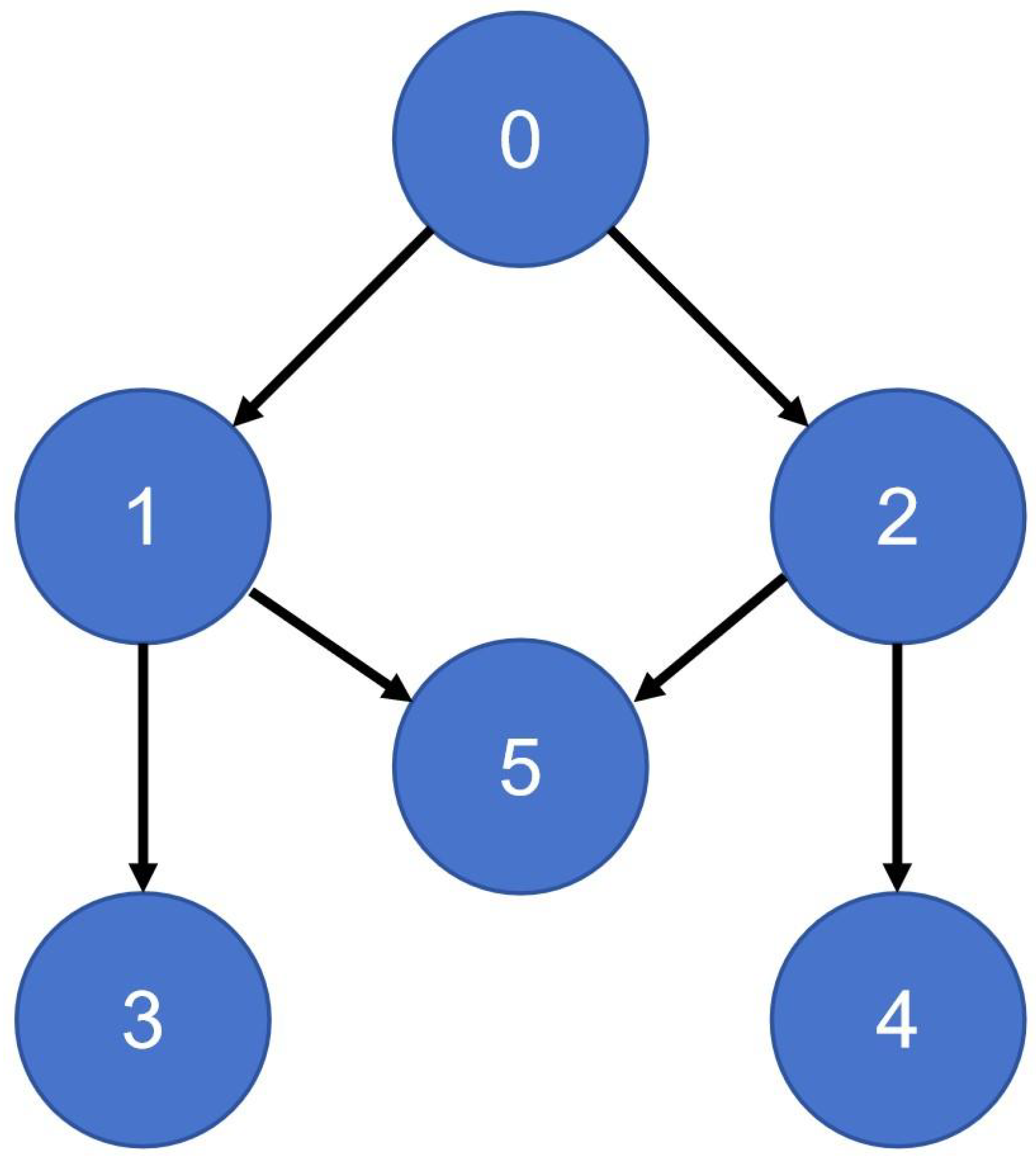
Consider an MAS consisting of one leader (indexed as node 0) and five followers (indexed as nodes 1–5). The directed communication topology is depicted in Figure 1.
The dynamics of the heterogeneous follower agents are described by
ξ ˙ 1 , i = ξ 2 , i + 1 1 + i ξ 1 , i 2 + 0.1 sin ( t ) ξ ˙ 2 , i = g i u f i + ξ 1 , i sin 1 i + ξ 2 , i 2 + 0.1 cos ( t )
where i = 1 , , 5 , and ξ 1 , i , ξ 2 , i R represent the system states.
The initial states of the five followers are selected as ξ 1 ( 0 ) = [ 6 , 1 ] T , ξ 2 ( 0 ) = [ 6 , 2 ] T , ξ 3 ( 0 ) = [ 3 , 3 ] T , ξ 4 ( 0 ) = [ 3 , 4 ] T , and ξ 5 ( 0 ) = [ 1 , 5 ] T . The leader output trajectory is selected as y 0 ( t ) = ξ 0 ( t ) = 5 sin ( 2 t ) , which corresponds to ξ ˙ 0 ( t ) = 10 cos ( 2 t ) . All adaptive parameters are initialized at 0.1 . The control and design parameters are configured as g i = 1 , q j , i = p j , i = 0.001 , τ i = 0.001 , and υ j , i = ι i = 0.001 for i = 1 , , 5 and j = 1 , 2 . For the finite-time differentiator (FTD), the design constants are set to c 1 = c 2 = 6 . The performance scaling function κ t p ( α , σ , t ) is parameterized with α = 2.5 , r = 0.5 , and σ = 0.01 .
The actuator fault profiles injected into the system are summarized in Table 1. Concretely, follower 1 experiences concurrent loss-of-effectiveness and time-varying bias faults, follower 3 undergoes a time-varying loss-of-effectiveness fault, while followers 2, 4, and 5 operate under fault-free conditions.
To investigate the influence of the prescribed time on transient tracking and control effort, two cases are considered, while all remaining parameters are kept unchanged:
Case 1 : t p = 2 s , Case 2 : t p = 0.5 s .
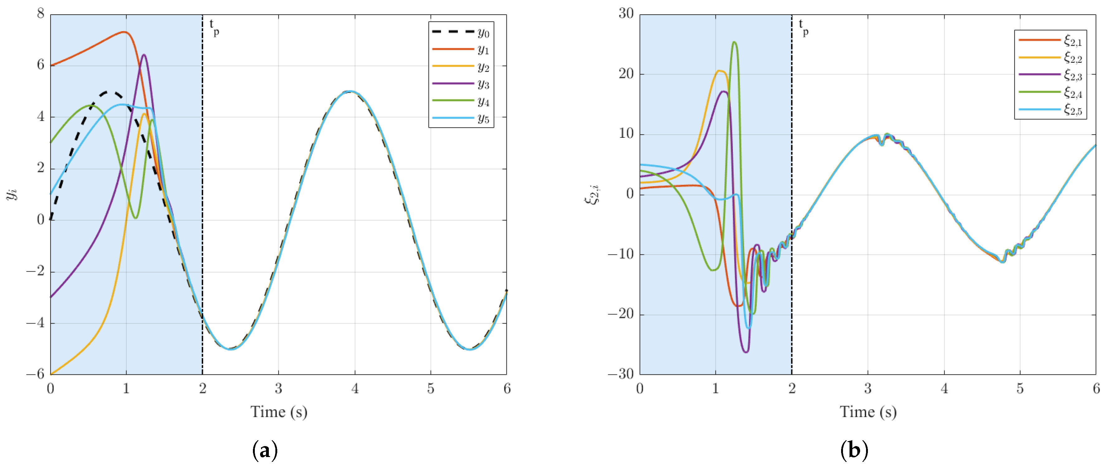
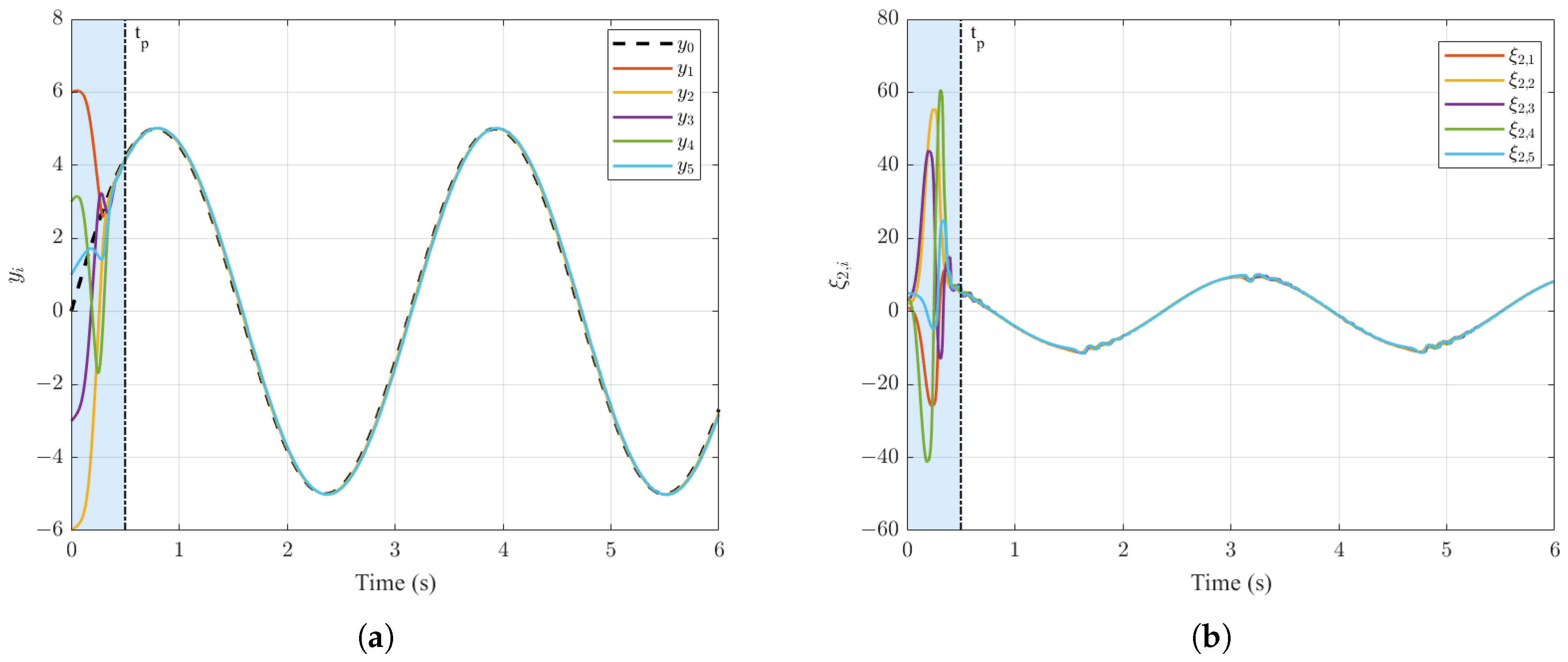
The responses of Example 1 are presented in Figure 2, Figure 3, Figure 4 and Figure 5. For t p = 2 s, Figure 2 shows that the follower outputs enter a small neighborhood of the leader trajectory by the assigned time, while the second-state trajectories remain bounded. When the prescribed time is reduced to t p = 0.5 s, Figure 3 indicates a substantially faster transient response.
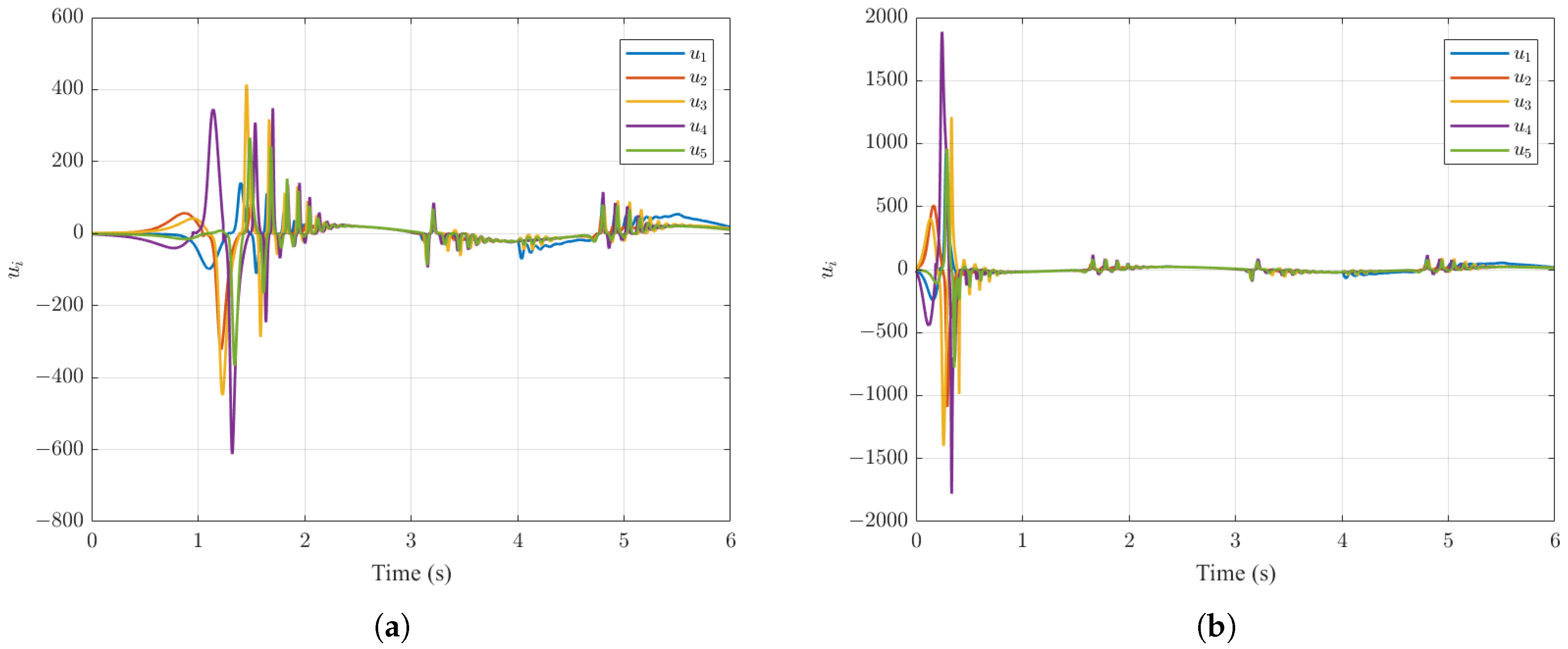
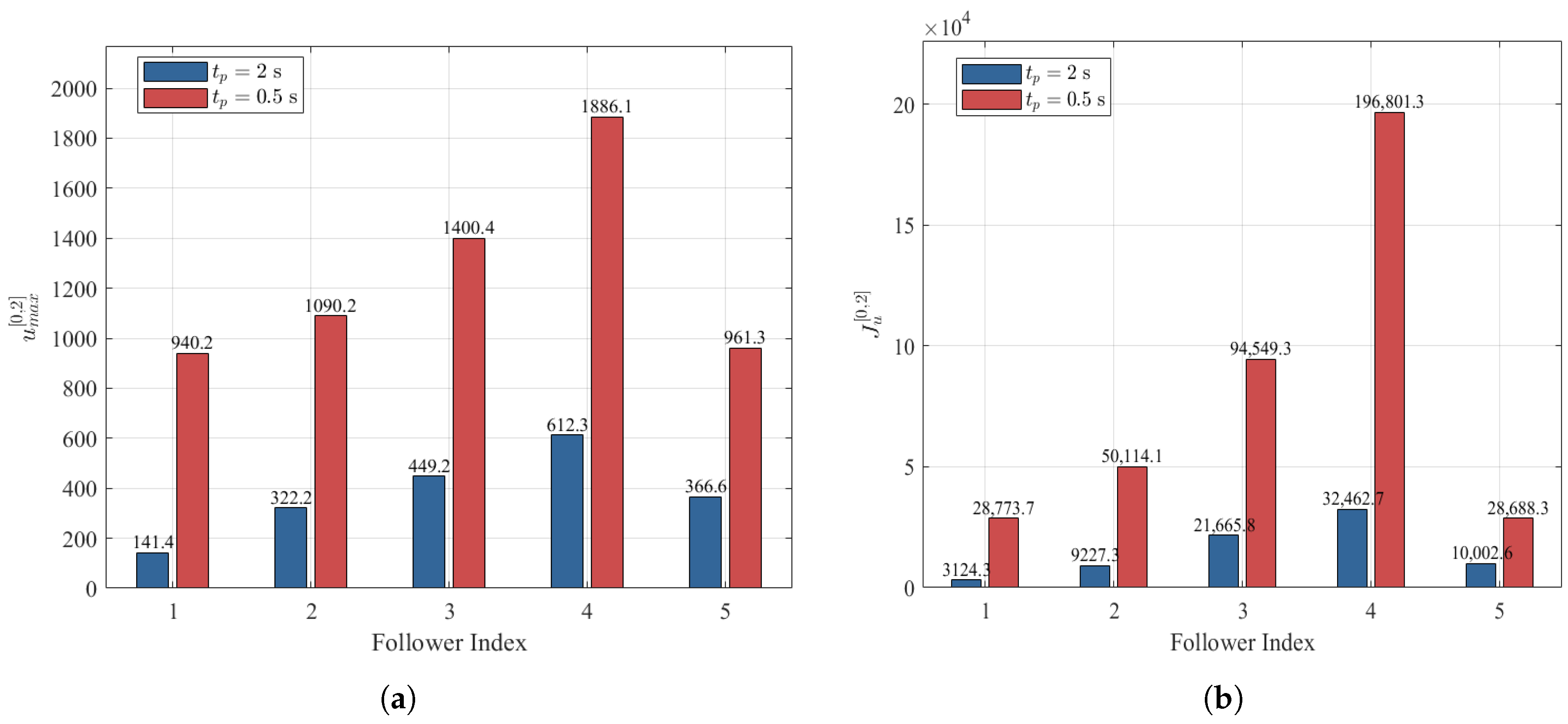
Figure 4 compares the commanded control inputs under the two prescribed-time settings. The shorter prescribed time results in markedly larger transient input peaks, which is consistent with the increased control demand required for rapid error reduction. To quantify this effect, define the per-agent indices
U max , i [ 0 , 2 ] = max 0 t 2 | u i ( t ) | , J u , i [ 0 , 2 ] = 0 2 u i 2 ( t ) d t , i = 1 , , 5 .
The interval [ 0 , 2 ] s contains both prescribed times and precedes the activation of the actuator faults in Table 1. Hence, the indices primarily characterize the transient control demand induced by the prescribed-time selection.
As shown in Figure 5, reducing t p from 2 s to 0.5 s increases both U max , i [ 0 , 2 ] and J u , i [ 0 , 2 ] for all followers in this simulation. For example, the maximum input magnitude of follower 4 increases from approximately 612.3 to 1886.1 , while its cumulative input energy increases from approximately 3.25 × 10 4 to 1.97 × 10 5 . These numerical observations indicate that the bounded scaling construction prevents singular time-varying gains, while faster prescribed-time responses still require increased transient input effort.

4.2. Example 2: Single-Link Robotic Manipulators

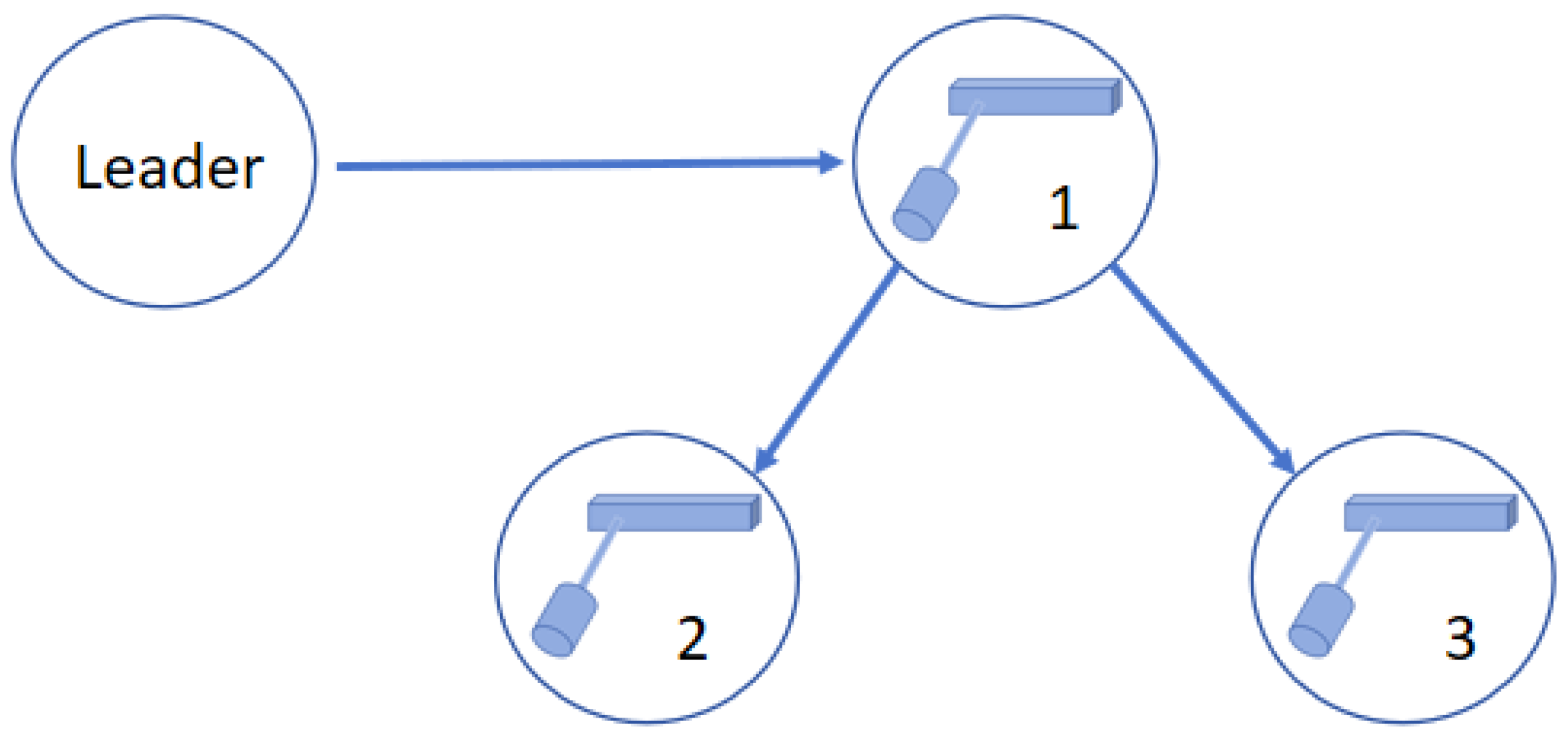
To examine the applicability of the proposed controller to an engineering-oriented nonlinear benchmark, consider a cooperative network of three single-link robotic manipulators. The communication topology is shown in Figure 6. The mathematical model describing the dynamics of the i-th manipulator is given by
M i z ¨ i + ω i z ˙ i + 1 2 m i g l i sin ( z i ) = τ i ,
where z i R represents the angular displacement, z ˙ i R denotes the angular velocity, and τ i R is the applied control torque. The structural parameters M i , ω i , m i , l i , and g denote the link inertia, viscous friction coefficient, link mass, physical link length, and gravitational acceleration, respectively.
By designating the system state variables as ξ i , 1 = M i z i and ξ i , 2 = M i z ˙ i , and treating the actuator-driven torque as the control input u i = τ i , the fault-actuated manipulator dynamics can be cast into the following state-space form:
ξ ˙ 1 , i = ξ 2 , i , ξ ˙ 2 , i = u f i ω i M i ξ 2 , i 1 2 m i g l i sin ξ 1 , i M i .
For comparative consistency, the actuator fault profiles injected into this three-agent manipulator system follow the exact formulation defined in Table 1 (applied to followers 1, 2, and 3). The mechanical constants are chosen uniformly as M i = 1.5 kg · m 2 , ω i = 1 N · m · s / rad , m i = 1 kg , and l i = 0.8 m for i = 1 , 2 , 3 , with the gravitational acceleration set to g = 9.81 m / s 2 .
The initial system states are set to ξ 1 ( 0 ) = [ 9 , 3 ] T , ξ 2 ( 0 ) = [ 7 , 2 ] T , and ξ 3 ( 0 ) = [ 5 , 1 ] T , while all adaptive estimation variables are initialized at 0.1 . The leader state is generated by ξ ˙ 0 = sin ( t ) , ξ 0 ( 0 ) = 0 . The controller configuration parameters are selected as q j , i = p j , i = 0.01 , τ i = 0.005 , and υ j , i = ι i = 0.01 for i = 1 , 2 , 3 and j = 1 , 2 . The FTD gains are maintained at c 1 = c 2 = 6 . For the performance scaling function κ t p ( α , σ , t ) , the design parameters are selected as α = 1 , r = 0.2 , and σ = 0.01 . The system is evaluated under two distinct convergence speed requirements: Case 1 ( t p = 3.0 s) and Case 2 ( t p = 6.0 s).
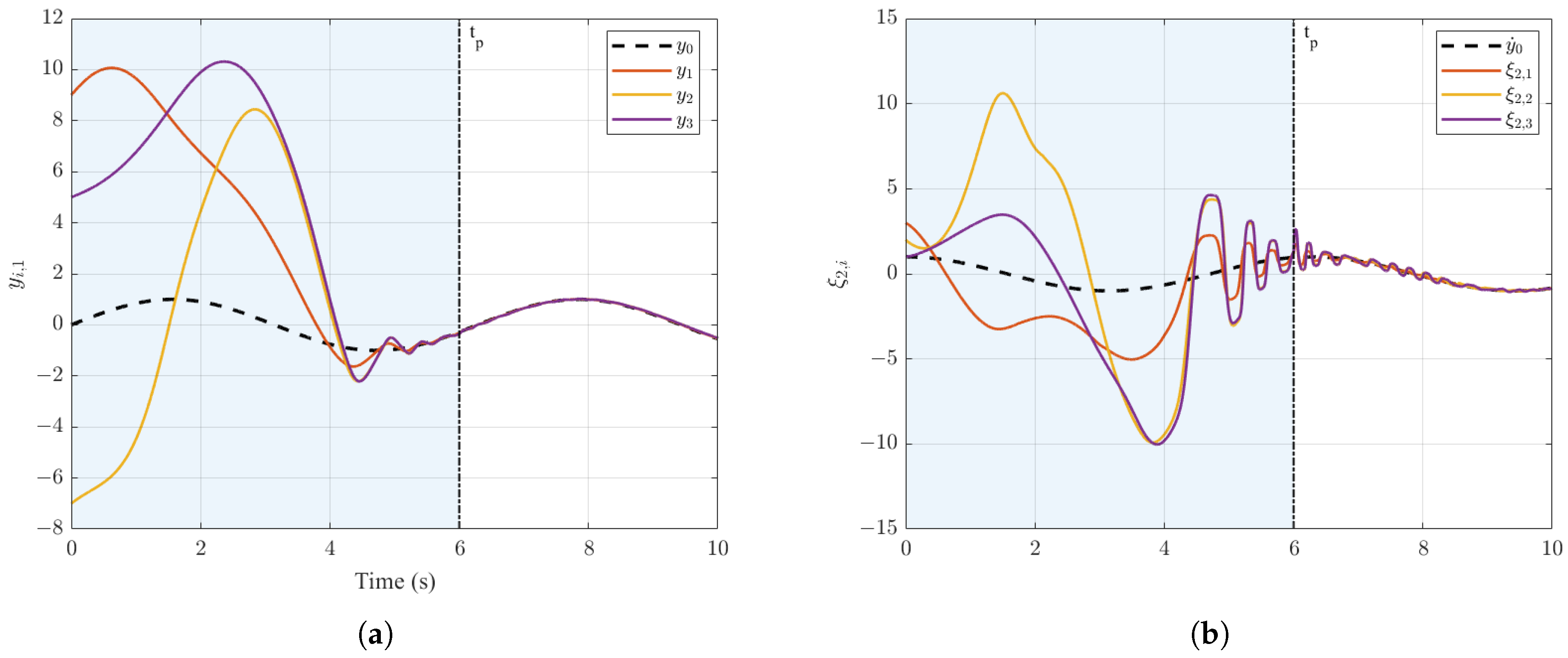
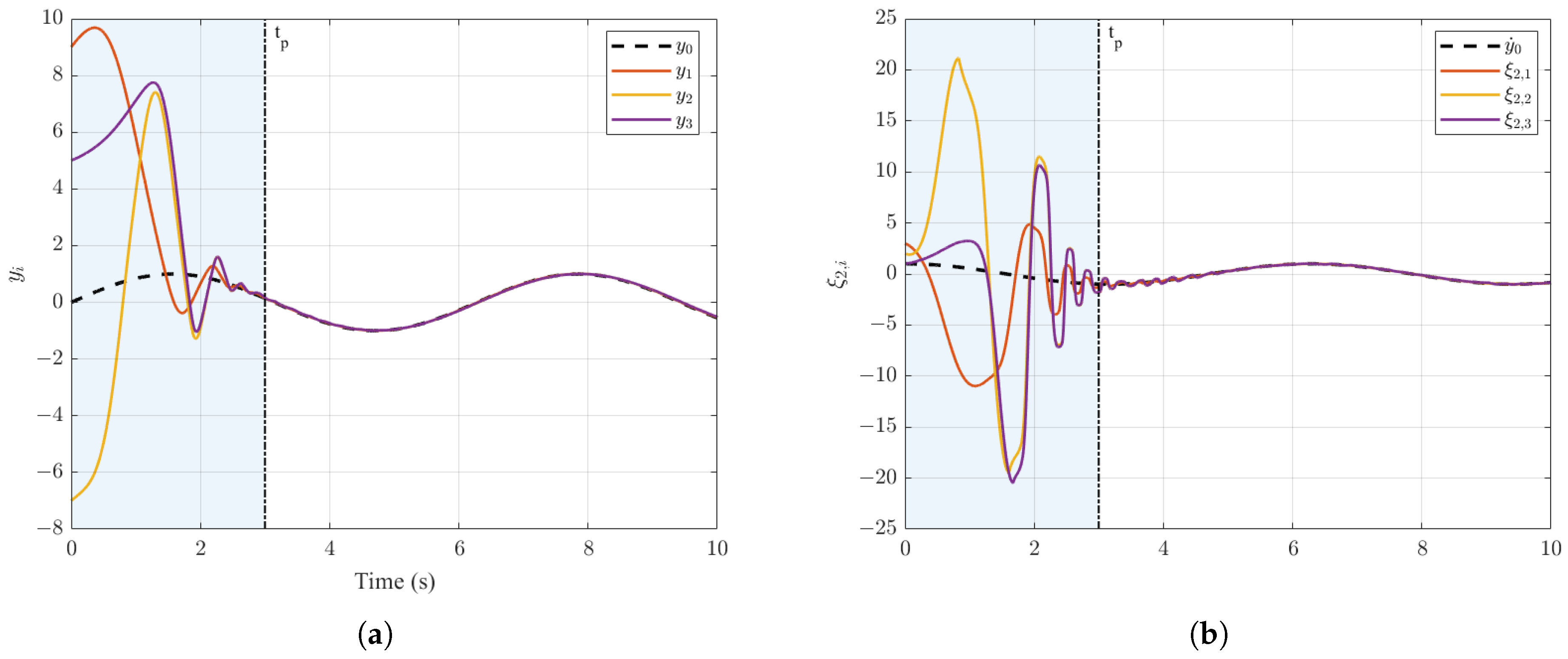
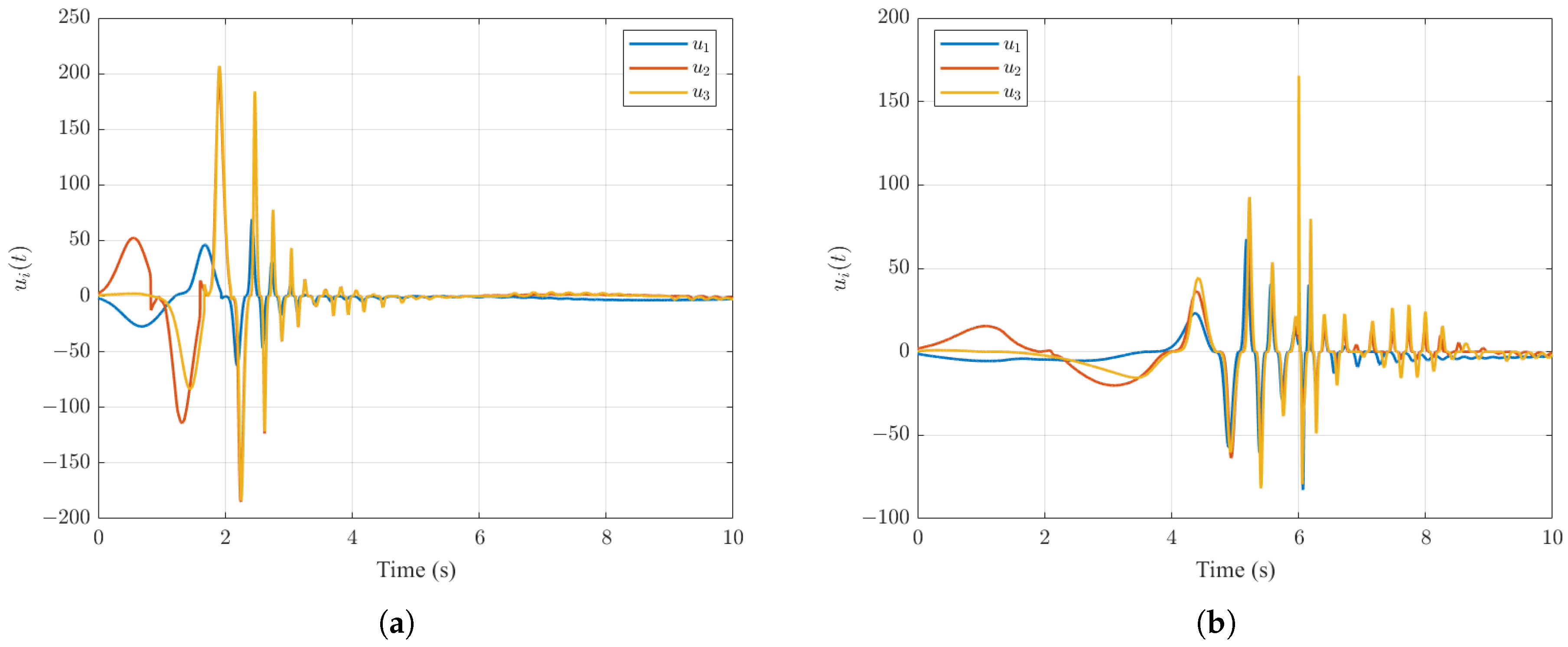
Figure 7, Figure 8, Figure 9 and Figure 10 present the responses of the robotic-manipulator example. For Case 1 with t p = 3 s, Figure 7 shows that the manipulator outputs enter a small neighborhood of the leader trajectory by the assigned time, while the second-state trajectories remain bounded. For Case 2 with t p = 6 s, Figure 8 indicates a slower but less aggressive transient response under the relaxed prescribed-time setting.
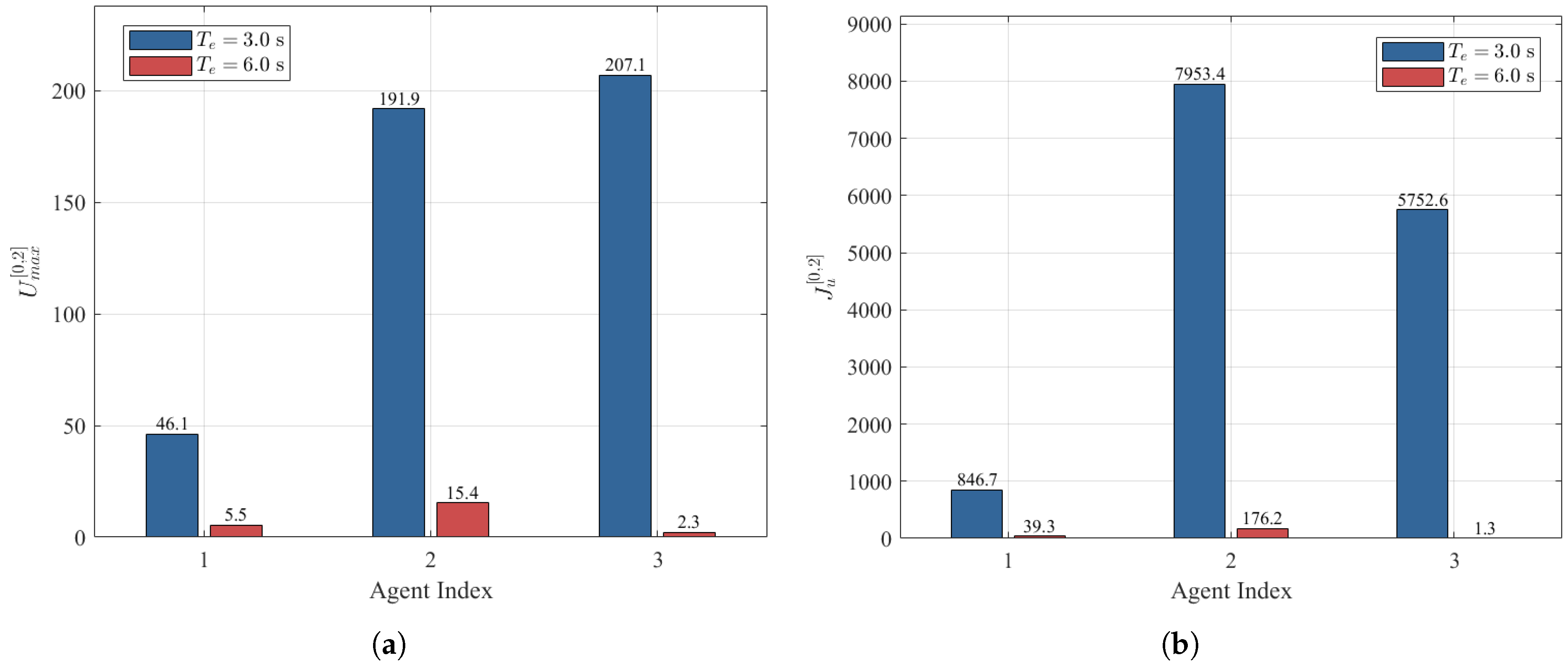
Figure 9 compares the commanded control inputs under the two prescribed times. The shorter setting t p = 3 s produces larger initial input peaks, whereas increasing the prescribed time to t p = 6 s reduces the early transient control demand. To quantify this behavior, define
U max , i [ 0 , 2 ] = max 0 t 2 | u i ( t ) | , J u , i [ 0 , 2 ] = 0 2 u i 2 ( t ) d t , i = 1 , 2 , 3 .
The interval [ 0 , 2 ] s precedes the actuator-fault activation instants and therefore isolates the early control effort induced by the prescribed-time selection. As shown in Figure 10, the shorter prescribed-time setting requires larger initial control magnitudes and higher cumulative input energies for the simulated manipulators.
These numerical results illustrate the prescribed-time tracking and control-effort behavior of the proposed method on an engineering-oriented nonlinear benchmark under the selected operating conditions. They are not intended to establish universal superiority over existing fault-tolerant control schemes.

5. Conclusions

This study addressed PT bounded consensus tracking for HONMASs affected by actuator faults, uncertain nonlinear dynamics, and unmatched disturbances. A bounded-scaling PT condition was combined with an adaptive NN-based backstepping design to obtain a nonsingular fault-tolerant control framework. Theoretical analysis shows that the closed-loop signals remain bounded and that the output tracking errors enter an adjustable residual neighborhood within the prescribed time. The numerical examples illustrate the resulting tracking behavior under the selected operating conditions. Future work will consider systematic comparisons with related FTC schemes, hardware-oriented validation, and extensions to networks with switching topologies, output constraints, and cyber-attacks.

Author Contributions

Methodology, L.Z. and S.C.; validation, L.Z., S.C. and H.J.; formal analysis, L.Z.; data curation, L.Z. and H.J.; writing—original draft preparation, L.Z.; writing—review and editing, L.Z., S.C. and H.J.; supervision, S.C.; project administration, L.Z. and S.C. All authors have read and agreed to the published version of the manuscript.

Funding

This research was funded by the National Natural Science Foundation of China, grant number 62263011; and the Scientific Research Project of Universities in Anhui Province, grant numbers 2023AH051386 and 2025AHGXZK20008.

Data Availability Statement

The raw data supporting the conclusions of this article will be made available by the authors on request.

Conflicts of Interest

The authors declare no conflicts of interest.

References

  1. Xu, T.; Yi, X.; Wen, G. Distributed fuzzy formation control of multi-UAV systems with directed communication networks. IEEE Trans. Fuzzy Syst. 2025, 33, 3582–3594. [Google Scholar] [CrossRef] [Scilit]
  2. Yu, Z.; Qu, Y.; Zhang, Y. Distributed fault-tolerant cooperative control for multi-UAVs under actuator fault and input saturation. IEEE Trans. Control Syst. Technol. 2019, 27, 2417–2429. [Google Scholar] [CrossRef] [Scilit]
  3. Li, X.; Wen, C.; Chen, C.; Xu, Q. Adaptive resilient secondary control for microgrids with communication faults. IEEE Trans. Cybern. 2022, 52, 8493–8503. [Google Scholar] [CrossRef] [Scilit]
  4. Zhang, W.; Qian, T.; Chen, X.; Huang, K.; Tang, W.; Wu, Q. Resilient economic control for distributed microgrids under false data injection attacks. IEEE Trans. Smart Grid 2021, 12, 4435–4446. [Google Scholar] [CrossRef] [Scilit]
  5. Ning, B.; Han, Q.-L.; Lu, Q. Fixed-time leader-following consensus for multiple wheeled mobile robots. IEEE Trans. Cybern. 2020, 50, 4381–4392. [Google Scholar] [CrossRef] [Scilit]
  6. Peng, J.; Zhang, X.; Wang, Y.; Liu, J. Consensus formation control of wheeled mobile robots with mixed disturbances. J. Frankl. Inst. 2024, 361, 106932. [Google Scholar] [CrossRef] [Scilit]
  7. Luo, D.; Wang, Y.; Lewis, F.L.; Song, Y. Unified output-feedback-based prescribed performance consensus tracking control of heterogeneous multi-agent systems. IEEE/CAA J. Autom. Sin. 2025, 12, 1636–1647. [Google Scholar] [CrossRef] [Scilit]
  8. Tan, X.; Hu, C.; Cao, G.; Wei, Q.; Li, W.; Han, B. Fixed-time antidisturbance consensus tracking for nonlinear multiagent systems with matching and mismatching disturbances. IEEE/CAA J. Autom. Sin. 2024, 46, 1410–1423. [Google Scholar] [CrossRef] [Scilit]
  9. Zhang, K.; Zhou, B.; Wen, G. Global leader-following consensus of double-integrator multiagent systems by fully distributed bounded linear protocols. IEEE Trans. Autom. Control 2022, 67, 4846–4853. [Google Scholar] [CrossRef] [Scilit]
  10. Modares, H.; Kiumarsi, B.; Lewis, F.L.; Ferrese, F.; Davoudi, A. Resilient and robust synchronization of multiagent systems under attacks on sensors and actuators. IEEE Trans. Cybern. 2020, 50, 1240–1250. [Google Scholar] [CrossRef] [Scilit]
  11. Huang, J.; Dou, L.; Fang, H.; Chen, J. Distributed backstepping-based adaptive fuzzy control of multiple high-order nonlinear dynamics. Nonlinear Dyn. 2015, 8, 63–75. [Google Scholar] [CrossRef] [Scilit]
  12. Zhao, X.; Chen, S.; Zhang, Z.; Zheng, Y. Consensus tracking for high-order uncertain nonlinear MASs via adaptive backstepping approach. IEEE Trans. Cybern. 2023, 53, 1248–1259. [Google Scholar] [CrossRef] [Scilit]
  13. Wang, G.; Wang, C.; Li, L. Fully distributed low-complexity control for nonlinear strict-feedback multiagent systems with unknown dead-zone inputs. IEEE Trans. Syst. Man Cybern. Syst. 2020, 50, 421–431. [Google Scholar] [CrossRef] [Scilit]
  14. Zhao, X.; Chen, S.; Zhang, Z.; Zheng, Y. Observer-based adaptive scaled tracking control for nonlinear MASs via command-filtered backstepping. IEEE Trans. Syst. Man Cybern. Syst. 2023, 53, 425–437. [Google Scholar] [CrossRef] [Scilit]
  15. Yao, D.; Dou, C.; Yue, D.; Zhao, N.; Zhang, T. Adaptive neural network consensus tracking control for uncertain multi-agent systems with predefined accuracy. Nonlinear Dyn. 2020, 101, 2249–2262. [Google Scholar] [CrossRef] [Scilit]
  16. Shang, Y.; Chen, B.; Lin, C. Consensus tracking control for distributed nonlinear multiagent systems via adaptive neural backstepping approach. IEEE Trans. Syst. Man Cybern. Syst. 2020, 50, 2436–2444. [Google Scholar] [CrossRef] [Scilit]
  17. Sun, J.; Liu, C. Distributed fuzzy adaptive backstepping optimal control for nonlinear multimissile guidance systems with input saturation. IEEE Trans. Fuzzy Syst. 2019, 27, 447–461. [Google Scholar]
  18. Cao, Y.; Ren, W.; Meng, Z. Decentralized finite-time sliding mode estimators and their applications in decentralized finite-time formation tracking. Syst. Control Lett. 2010, 59, 522–529. [Google Scholar] [CrossRef] [Scilit]
  19. Zhao, Y.; Liu, Y.; Wen, G.; Huang, T. Finite-time distributed average tracking for second-order nonlinear systems. IEEE Trans. Neural Netw. Learn. Syst. 2019, 30, 1780–1789. [Google Scholar] [CrossRef] [Scilit] [PubMed]
  20. Liu, D.; Liu, Z.; Chen, C.L.; Zhang, Y. Finite-time distributed cooperative control for heterogeneous nonlinear multi-agent systems with unknown input constraints. Neurocomputing 2020, 415, 123–134. [Google Scholar] [CrossRef] [Scilit]
  21. Chen, D.; Liu, X.; Yu, W. Finite-time fuzzy adaptive consensus for heterogeneous nonlinear multi-agent systems. IEEE Trans. Netw. Sci. Eng. 2020, 7, 3057–3066. [Google Scholar] [CrossRef] [Scilit]
  22. Liu, Y.J.; Shang, X.; Tang, L.; Zhang, S. Finite-time consensus adaptive neural network control for nonlinear multiagent systems under PDE models. IEEE Trans. Neural Netw. Learn. Syst. 2025, 36, 6218–6228. [Google Scholar] [CrossRef] [Scilit]
  23. Zhang, D.; Chen, H.; Lu, Q.; Feng, G. Finite-time cooperative output regulation of heterogeneous nonlinear multi-agent systems under switching DoS attacks. Automatica 2025, 173, 112062. [Google Scholar] [CrossRef] [Scilit]
  24. Polyakov, A.; Efimov, D.; Perruquetti, W. Finite-time and fixed-time stabilization: Implicit Lyapunov function approach. Automatica 2015, 51, 332–340. [Google Scholar] [CrossRef] [Scilit]
  25. Tian, B.; Lu, H.; Zuo, Z.; Yang, W. Fixed-time leader–follower output feedback consensus for second-order multiagent systems. IEEE Trans. Cybern. 2019, 49, 1545–1550. [Google Scholar] [CrossRef] [Scilit]
  26. Zhang, L.; Chen, B.; Lin, C.; Shang, Y. Fuzzy adaptive fixed-time consensus tracking control of high-order multi-agent systems. IEEE Trans. Fuzzy Syst. 2022, 30, 567–578. [Google Scholar] [CrossRef] [Scilit]
  27. Cao, L.; Cheng, Z.; Liu, Y.; Li, H. Event-based adaptive NN fixed-time cooperative formation for multiagent systems. IEEE Trans. Neural Netw. Learn. Syst. 2024, 25, 6467–6477. [Google Scholar] [CrossRef] [Scilit]
  28. Song, Y.; Wang, Y.; Holloway, J.; Krstic, M. Time-varying feedback for regulation of normal-form nonlinear systems in prescribed finite time. Automatica 2017, 83, 243–251. [Google Scholar] [CrossRef] [Scilit]
  29. Wang, Y.; Song, Y.; Hill, D.J.; Krstic, M. Prescribed-time consensus and containment control of networked multiagent systems. IEEE Trans. Cybern. 2019, 49, 1138–1147. [Google Scholar] [CrossRef] [Scilit]
  30. Ding, T.F.; Ge, M.F.; Xiong, C.; Liu, Z.-W.; Ling, G. Prescribed-time formation tracking of second-order multi-agent networks with directed graphs. Automatica 2023, 154, 110997. [Google Scholar] [CrossRef] [Scilit]
  31. Qian, C.; Yu, Z.; Jiang, H.; Luo, Y. Prescribed-time leader-following scaled consensus for high-order nonlinear multi-agent systems. Nonlinear Dyn. 2025, 113, 24751–24770. [Google Scholar] [CrossRef] [Scilit]
  32. Ning, B.; Han, Q.; Zuo, Z. Practical fixed-time consensus for integrator-type multi-agent systems: A time base generator approach. Automatica 2019, 105, 406–414. [Google Scholar] [CrossRef] [Scilit]
  33. Zou, A.; Liu, Y.; Hou, Z.; Hu, Z. Practical predefined-time output-feedback consensus tracking control for multiagent systems. IEEE Trans. Cybern. 2023, 53, 5311–5322. [Google Scholar] [CrossRef] [Scilit]
  34. Luo, D.; Wang, Y.; Song, Y. Practical prescribed time tracking control with bounded time-varying gain under non-vanishing uncertainties. IEEE/CAA J. Autom. Sin. 2024, 11, 219–230. [Google Scholar] [CrossRef] [Scilit]
  35. Gallehdari, Z.; Meskin, N.; Khorasani, K. A distributed control reconfiguration and accommodation for consensus achievement of multiagent systems subject to actuator faults. IEEE Trans. Control Syst. Technol. 2016, 24, 2031–2047. [Google Scholar] [CrossRef] [Scilit]
  36. Khalili, M.; Zhang, X.; Polycarpou, M.; Polycarpou, T.; Cao, Y. Distributed adaptive fault-tolerant control of uncertain multi-agent systems. Automatica 2018, 87, 142–151. [Google Scholar] [CrossRef] [Scilit]
  37. Deng, C.; Yang, G. Distributed adaptive fault-tolerant control approach to cooperative output regulation for linear multi-agent systems. Automatica 2019, 103, 62–68. [Google Scholar] [CrossRef] [Scilit]
  38. Wu, W.; Tong, S. Fuzzy adaptive consensus control for nonlinear multiagent systems with intermittent actuator faults. IEEE Trans. Cybern. 2023, 53, 2969–2979. [Google Scholar] [CrossRef] [Scilit]
  39. Rotondo, D.; Theilliol, D.; Ponsart, J.-C. Virtual actuator and sensor fault tolerant consensus for homogeneous linear multi-agent systems. IEEE Trans. Circuits Syst. I Regul. Pap. 2024, 71, 1324–1334. [Google Scholar] [CrossRef] [Scilit]
  40. Dong, G.; Li, H.; Ma, H.; Lu, R. Finite-time consensus tracking neural network FTC of multi-agent systems. IEEE Trans. Neural Netw. Learn. Syst. 2021, 32, 653–662. [Google Scholar] [CrossRef] [Scilit]
  41. Zhang, P.; Xue, H.; Gao, S.; Zuo, X.; Zhang, J. Finite-time adaptive cooperative fault-tolerant control for multi-agent system with hybrid actuator faults. IEEE Syst. J. 2022, 16, 3590–3601. [Google Scholar] [CrossRef] [Scilit]
  42. Ren, H.; Ma, H.; Li, H.; Wang, Z. Adaptive fixed-time control of nonlinear MASs with actuator faults. IEEE/CAA J. Autom. Sin. 2023, 8, 1252–1262. [Google Scholar] [CrossRef] [Scilit]
  43. Lu, L.T.; Zhu, S.L.; Wang, D.M.; Han, Y.Q. Predefined-time adaptive consensus control for nonlinear multi-agent systems with input quantization and actuator faults. Nonlinear Dyn. 2024, 112, 14215–14234. [Google Scholar] [CrossRef] [Scilit]
  44. Zou, Z.; Wang, C. Adaptive trajectory tracking control of output constrained multi-rotors systems. IET Control Theory Appl. 2014, 8, 1163–1174. [Google Scholar]
Figure 1. Directed communication topology of the heterogeneous MASs in Example 1.
Mathematics 14 01919 g001
Figure 2. Responses of Example 1 with t p = 2 s: (a) follower outputs y i = ξ 1 , i and leader output y 0 ; (b) second-state trajectories ξ 2 , i . The shaded area indicates the prescribed-time interval [ 0 , t p ] .
Mathematics 14 01919 g002
Figure 3. Responses of Example 1 with t p = 0.5 s: (a) follower outputs y i = ξ 1 , i and leader output y 0 ; (b) second-state trajectories ξ 2 , i . The shaded area indicates the prescribed-time interval [ 0 , t p ] .
Mathematics 14 01919 g003
Figure 4. Commanded control inputs of Example 1 under different prescribed times: (a) t p = 2 s; (b) t p = 0.5 s.
Mathematics 14 01919 g004
Figure 5. Per-agent control-effort comparison for Example 1 over t [ 0 , 2 ] s: (a) maximum commanded-input magnitude U max , i [ 0 , 2 ] ; (b) cumulative commanded-input energy J u , i [ 0 , 2 ] .
Mathematics 14 01919 g005
Figure 6. Directed communication topology of the robotic-manipulator network in Example 2. The numbers denote the labels of the follower robotic manipulators.
Mathematics 14 01919 g006
Figure 7. Responses of the robotic-manipulator network with t p = 3 s: (a) manipulator outputs y i = ξ 1 , i and leader output y 0 ; (b) second-state trajectories ξ 2 , i . The shaded area indicates the prescribed-time interval [ 0 , t p ] .
Mathematics 14 01919 g007
Figure 8. Responses of the robotic-manipulator network with t p = 6 s: (a) manipulator outputs y i = ξ 1 , i and leader output y 0 ; (b) second-state trajectories ξ 2 , i . The shaded area indicates the prescribed-time interval [ 0 , t p ] .
Mathematics 14 01919 g008
Figure 9. Commanded control inputs of Example 2 under different prescribed times: (a) t p = 3 s; (b) t p = 6 s.
Mathematics 14 01919 g009
Figure 10. Per-manipulator control-effort comparison for Example 2 over t [ 0 , 2 ] s: (a) maximum commanded-input magnitude U max , i [ 0 , 2 ] ; (b) cumulative commanded-input energy J u , i [ 0 , 2 ] .
Mathematics 14 01919 g010
Table 1. Actuator fault profiles of the follower agents (Example 1).
Follower β i ( t ) μ i ( t )
1 1 , t < 4 s , 0.2 sin ( t ) + 0.6 , t 4 s , 0 , t < 3 s , 2 sin ( t ) + 1 , t 3 s ,
210
3 1 , t < 5 s , 0.7 0.3 sin ( t ) , t 5 s , 0
410
510
Disclaimer/Publisher’s Note: The statements, opinions and data contained in all publications are solely those of the individual author(s) and contributor(s) and not of MDPI and/or the editor(s). MDPI and/or the editor(s) disclaim responsibility for any injury to people or property resulting from any ideas, methods, instructions or products referred to in the content.