(d, c, l)-Privacy: Privacy Preservation Models for Content-Based Datasets Using Information Retrieval Techniques

Abstract

The release of datasets containing sensitive user information requires a careful balance between data utility and privacy preservation. To address this challenge, numerous privacy preservation models have been proposed, including k-Anonymity, l-Diversity, t-Closeness, and Differential privacy. However, these models are largely designed for simple datasets in which each attribute is represented by a single (atomic) value, limiting their effectiveness in more complex data environments. Specifically, k-Anonymity and its variants have been widely adopted to mitigate privacy risks arising from quasi-identifier-based inference attacks. While l-Diversity and t-Closeness are extended from k-Anonymity to address the disclosure of sensitive attributes. However, they are primarily effective when sensitive attributes are singular and well defined, which restricts their applicability in scenarios involving complex or content-based data. Another prominent approach is Differential privacy and its variants, which rely on probabilistic mechanisms and the introduction of random noise into query outputs. It provides strong theoretical guarantees and is well suited for numerical data and computation-driven applications. However, it is also less effective for content-based datasets, where semantic meaning and contextual integrity are essential and cannot be preserved through randomization. To overcome these limitations, this study proposes a new privacy preservation model, $(d,c,l)$-Privacy, specifically designed for content-based datasets. The proposed model ensures that released datasets satisfy the constraints defined by parameters d, c, and l, thereby mitigating potential privacy violations. To enforce these constraints, three algorithms are introduced, i.e., FCFS, greedy, and optimal $(d,c,l)$-privacy algorithms. The FCFS algorithm prioritizes computational efficiency while maintaining acceptable privacy guarantees. The greedy algorithm balances execution time and data utility. While the optimal algorithm focuses on maximizing semantic preservation and overall data usefulness, albeit at a higher computational cost. Experimental results show that the proposed algorithms effectively mitigate privacy risks in released datasets under $(d,c,l)$-privacy constraints. Among the evaluated algorithms, FCFS achieves the highest computational efficiency, while the greedy algorithm provides a favorable trade-off between efficiency and data utility. The optimal algorithm consistently delivers the highest level of data quality, despite increased computational overhead. These findings indicate that the proposed model and algorithms provide an effective and practical solution for privacy preservation data publishing in real-world, content-based data environments.

1. Introduction

The online assessment is a tool that is available in real-life applications. Generally, they are used to survey and collect information on the satisfaction of customers or users with services, products, and applications that are provided. The information is collected from the online assessment, which often consists of two types of questions, i.e., multiple-choice questions (MCQ) and open-ended questions (OEQ). Moreover, the questions of online assessments are generally divided into three groups, i.e., demographic questions, behavioral and satisfaction questions, and source questions. Generally, this information is used to improve customer services, organizational policies, or marketing policies. For this reason, they are often released to the data analyst. Thus, they could lead to concerns about privacy violations. To address these concerns, in [1] and its extended versions [2,3,4,5,6,7], the authors recommend that all users’ explicit identifier values (e.g., citizen, SSN, and student code) are removed, and all unique quasi-identifier values are suppressed or generalized by their less specific values to be indistinguishable.

An illustrative example of privacy preservation using k-Anonymity [1] is presented for the case where the anonymity parameter k is set to 2. Let

Table 1. An example of an original dataset with explicit identifiers, quasi-identifiers, and a sensitive attribute.

Tuple	Explicit Identifier	Quasi-Identifiers				Sensitive
	SSN	Name	Gender	Education	Position	Salary
$d_1$	010-034-2589	Emma	Female	Master’s degree	Accounting	$9500.00
$d_2$	010-034-4561	Jennifer	Female	Bachelor’s degree	Accounting	$7000.00
$d_3$	223-231-3210	Bob	Male	Master’s degree	Programmer	$7000.00
$d_4$	237-246-7412	Alice	Female	Master’s degree	Programmer	$12,000.00

denote the original dataset. In this dataset, SSN and Name serve as explicit identifiers, while Gender, Education, and Position are quasi-identifier attributes. Salary is treated as a sensitive attribute. To achieve privacy preservation, all values corresponding to the explicit identifiers (SSN and Name) are removed. In addition, the values of the quasi-identifier attributes—Gender, Education, and Position—are generalized such that each combination appears in at least two indistinguishable tuples. Under these transformations, the released version of Table 1 satisfies the requirements of 2-Anonymity, as shown in

Table 2. A 2-Anonymity version of Table 1 after removing explicit identifiers and generalizing quasi-identifier values.

Tuple	Quasi-Identifiers			Sensitive
	Gender	Education	Position	Salary
$d_1$	Female	*	Accounting	$9500.00
$d_2$	Female	*	Accounting	$7000.00
$d_3$	*	Master’s degree	Programmer	$7000.00
$d_4$	*	Master’s degree	Programmer	$12,000.00

* denotes a quasi-identifier value that has been generalized.

. From Table 2, it can be observed that for any query based on quasi-identifier attributes, at least two tuples satisfy the query conditions, thereby preventing unique tuple re-identification. As a result, the released dataset in Table 2 provides stronger privacy protection against re-identification attacks compared with the original dataset shown in Table 1. Unfortunately, they continue to exhibit notable limitations, including degradation of data utility and vulnerability to emerging privacy attack techniques introduced after their deployment.

In addition to datasets in which each attribute is designed to collect atomic values (e.g., Table 1), certain datasets are constructed to capture information in the form of user-generated textual contents, such as feedback, opinions, or discussion statements. Such datasets are referred to as content-based datasets. An example of content-based datasets is presented in

Table 3. An example of a content-based dataset collecting student opinions, where Student Code is an explicit identifier, Datetime, Education, and Gender are quasi-identifiers, and Opinion is the sensitive content-based attribute.

Tuple	Explicit Identifier	Sensitive	Quasi-Identifier
	Student Code	Opinion	Datetime	Education	Gender
$d_1$	STU123	You are a worst lecturer that I’ve ever met because you never listen to my efforts to explain the reasons behind the problems I’ve encountered, fuck you, bad lecturer, bad lecturer, …, and very bad lecturer.	2023-07-03	Bachelor’s degree	Female
$d_2$	STU456	You are a good lecturer. I love and respect you. Moreover, I would like to study with you again. However, I heard that you are a bad lecturer with someone.	2023-06-15	Master’s degree	Male
$d_3$	STU789	A good lecturer.	2023-06-15	Master’s degree	Male
$d_4$	STU246	He is a good lecturer and a nice man.	2023-06-15	Bachelor’s degree	Male

. In this dataset, Student Code serves as the explicit identifier, while Datetime, Education, and Gender are treated as quasi-identifier attributes. The Opinion attribute contains sensitive information that must be protected when Table 3 is released beyond the scope of the data-collecting organization. Notably, beyond explicitly sensitive content, the Opinion attribute itself could also facilitate re-identification of the data owner. This is because user-generated textual content often embeds distinctive linguistic styles, personal viewpoints, and affective expressions that can uniquely characterize its author. As a result, even after removing the Student Code and generalizing the quasi-identifier attributes (Datetime, Education, and Gender), privacy concerns may persist. Therefore, merely applying k-Anonymity and its well-known extensions, including l-Diversity and t-Closeness [1,2,3,4,5,6,7], to such datasets is insufficient to fully mitigate privacy violation concerns in content-based datasets. While these models protect against identity disclosure based on structured attributes, they fail to address privacy leakage arising from the semantic and stylistic characteristics inherent in textual content.

An illustrative case highlighting privacy violation concerns in content-based datasets is presented using Table 3 as the specified original dataset. This table is assumed to collect students’ comments directed toward Bob. To preserve privacy using k-Anonymity, the anonymity parameter is set to k = 2. Accordingly, a released version of Table 3 that satisfies the 2-Anonymity constraint is shown in

Table 4. A data version of Table 3 is satisfied by 2-Anonymity.

Tuple	Sensitive	Quasi-Identifier
	Opinion	Datetime	Education	Gender
$d_1$	You are a worst lecturer that I’ve ever met because you never listen to my efforts to explain the reasons behind the problems I’ve encountered, fuck you, bad lecturer, bad lecturer, …, and very bad lecturer.	2023	Bachelor’s degree	*
$d_2$	You are a good lecturer. I love and respect you. Moreover, I would like to study with you again. However, I heard that you are a bad lecturer with someone.	2023-06-15	Master’s degree	Male
$d_3$	A good lecturer.	2023-06-15	Master’s degree	Male
$d_4$	He is a good lecturer and a nice man.	2023	Bachelor’s degree	*

* denotes a quasi-identifier value that has been generalized.

. As observed from Table 4, each tuple is indistinguishable from at least k − 1 other tuples with respect to the quasi-identifier attributes. Under this condition, the dataset appears to provide adequate privacy protection and to satisfy the requirements of 2-Anonymity. However, despite conforming to the 2-Anonymity constraint, the released dataset still exhibits privacy violation concerns arising from its content-based attributes. These residual privacy concerns are demonstrated in Example 1, indicating that k-Anonymity alone is insufficient for guaranteeing privacy protection in content-based datasets.

Example 1 (Privacy violation issues in content-based datasets).

Consider Table 4, which represents the 2-Anonymous release of the original content-based dataset shown in Table 3. Suppose Bob is a lecturer, and Alice and John are two of his students. One tuple in Table 4 corresponds to Alice’s opinion about Bob, and Alice is the target individual whose opinion Bob attempts to infer from the released dataset. Assume that Alice and John are involved in a conflict, and Bob has determined that Alice initiated the dispute. Furthermore, assume that Bob does not have conflicts with any other students. Under these circumstances, Bob can leverage this background knowledge to infer that the tuple $t_1$ in Table 4 is Alice’s opinion. This inference is possible because the content of the tuple $t_1$ is highly consistent with the known conflict among Alice, John, and Bob.

This example demonstrates that, even though Table 4 satisfies the 2-Anonymity constraint, privacy violations could still occur due to semantic inference enabled by external background knowledge. Consequently, k-Anonymity alone is insufficient to prevent privacy breaches in content-based datasets.

To address the limitations of k-Anonymity and its extended variants, numerous privacy preservation models have been proposed to mitigate privacy violation concerns in content-based datasets, particularly within the domains of Natural Language Processing (NLP)  [8,9,10,11] and Information Retrieval (IR) [12,13,14,15]. Representative examples of such privacy preservation models for content-based datasets are summarized in Table 5. These models have evolved from early privacy-aware query frameworks [16,17,18] and traditional data anonymization techniques [19,20,21,22], as well as TFIDF-based text clustering approaches [23,24,25,26,27], to more advanced mechanisms such as homomorphic encryption [28,29,30,31], differential privacy [32,33,34,35], and federated learning frameworks [36,37,38]. These approaches enhance sensitivity detection by incorporating semantic relevance and contextual rarity within textual content.

In addition, several paradigms have been pursued to address the privacy concerns described above, each adopting a different strategy for how the data are ultimately released. The first is anonymization-based publishing, which, as discussed above, includes k-Anonymity, l-Diversity, and t-Closeness; this paradigm releases a single sanitized table by generalizing or suppressing the original tuples, but the constraints are primarily defined over atomic quasi-identifier values and become difficult to enforce when sensitive information is expressed within free-form textual content. A second paradigm is the anatomy method [39,40,41], which releases the quasi-identifier and sensitive values as two separate tables linked by a group identifier so that individual-level correlations are obscured while aggregate-level analysis remains accurate; however, the split-table format breaks tuple-level readability and is therefore unsuited to downstream natural language processing or information retrieval analysis. A third paradigm operates through aggregate and query-answering frameworks, in which the data owner exposes only aggregated statistics, encrypted indices, or controlled query interfaces over the underlying tuples rather than releasing the dataset itself [16,17,18,28,29]; while this protects the raw tuples, it prevents third parties from inspecting or auditing the content of individual documents. A fourth paradigm is differential privacy and its variants [32,33,34,35], which inject calibrated random noise into query outputs or learned statistics; this provides rigorous probabilistic guarantees but tends to distort the semantic meaning and contextual integrity of textual content, making it less effective for content-based settings.

Table 5. Related work on privacy preservation for content-based datasets, organized by approach, key idea, and reference.

Model	Approach	Key Idea	Ref.
Using TF-IDF to hide sensitive itemsets	SIF-IDF Algorithm and Greedy Approach	Sanitizes sensitive items while maintaining data utility using text mining concepts.	[42]
TF-IDF and KDC-based Privacy Search	KDC and TF-IDF over Encrypted Data	Enables secure, ranked multi-keyword search on cloud-stored encrypted data.	[43]
Differential privacy protection via SVD	SVD-based Disturbance and Differential Privacy	Protects high-dimensional network data by disturbing singular values and spectral vectors.	[44]
Privacy-Preserving Collaborative Clustering	Privacy-Preserving Distributed Clustering	Multi-party document clustering without revealing raw sensitive text to the server.	[45]
Automatic Anonymization of Textual Documents	Word Embedding-based Semantic Detection	Detects sensitive information using semantic similarity in word embeddings.	[46]

Table 5. Related work on privacy preservation for content-based datasets, organized by approach, key idea, and reference.

Model	Approach	Key Idea	Ref.
Using TF-IDF to hide sensitive itemsets	SIF-IDF Algorithm and Greedy Approach	Sanitizes sensitive items while maintaining data utility using text mining concepts.	[42]
TF-IDF and KDC-based Privacy Search	KDC and TF-IDF over Encrypted Data	Enables secure, ranked multi-keyword search on cloud-stored encrypted data.	[43]
Differential privacy protection via SVD	SVD-based Disturbance and Differential Privacy	Protects high-dimensional network data by disturbing singular values and spectral vectors.	[44]
Privacy-Preserving Collaborative Clustering	Privacy-Preserving Distributed Clustering	Multi-party document clustering without revealing raw sensitive text to the server.	[45]
Automatic Anonymization of Textual Documents	Word Embedding-based Semantic Detection	Detects sensitive information using semantic similarity in word embeddings.	[46]

In parallel with these data-centric models, a substantial body of recent work has emerged around AI-based privacy preservation, in which deep learning, large language models (LLMs), and federated architectures are used either as the protection mechanism itself or as the adversary that motivates new defenses. Representative directions include differentially private deep learning and fine-tuning of pre-trained language models, language model-based text anonymization, deep generative models for privacy-preserving synthetic data, and federated learning frameworks with differential privacy or homomorphic encryption. These directions, together with their representative models and references, are summarized in

Table 6. Recent AI-based privacy preservation models, organized by model, approach, key idea, and reference.

Model	Approach	Key Idea	Ref.
DP-SGD/DP Deep Learning	Gradient clipping with Gaussian noise injection; parameter-efficient differentially private fine-tuning	Trains or fine-tunes deep neural networks (including large pre-trained language models) under $(\epsilon ,\delta )$-differential privacy to prevent leakage of training data through the released model.	[35,47,48]
Language model-based anonymization	Fine-tuned language models for named-entity recognition and de-identification	Detects direct and quasi-identifiers in textual documents using pre-trained language models and replaces them with placeholders, producing redacted but human-readable text.	[49,50,51]
Generative synthetic data	Deep generative models such as diffusion and language model-based generators for tabular data	Trains generative models on real datasets to produce synthetic tuples that approximate the underlying distribution, allowing dataset sharing without releasing original tuples.	[52,53,54]
Federated learning with differential privacy or homomorphic encryption	Local client training with secure aggregation of model updates	Enables multiple organizations to jointly train a model without sharing raw data, while protecting model updates through noise injection or cryptographic aggregation.	[55,56]

. Collectively, AI-based methods extend the privacy landscape from data-centric anonymization toward model-centric and learning-centric protections; however, their output is typically a privatized model or a synthetic dataset rather than a human-readable release of the original tuples, and they therefore do not address the problem of publishing real content-based datasets in a form that remains directly readable and analyzable by downstream users.

To address these limitations, this work proposes ($(d,c,l)$-Privacy: Privacy Preservation Models for Content-Based Datasets Using Information Retrieval Techniques. The proposed model directly releases a sanitized version of the original content-based tuples under explicit structural constraints on equivalence-class size (d), re-identification confidence (c), and sensitive-term occurrence (l), and is supported by three algorithms—FCFS, greedy, and optimal—that trade off computational efficiency and data utility.

The organization of this work is as follows. This section provides an introduction to this work. Section 2 introduces the proposed privacy preservation model, including the formal problem definition, term document measurement approaches, i.e., expert-based and mechanism-based measurements, data distortion techniques, and the $(d,c,l)$-Privacy model. Section 3 presents the experimental evaluation of the proposed approach under various settings. Finally, Section 4 and Section 5 summarize the conclusions and outline directions for future work, respectively.

2. The Proposed Model

Before presenting the proposed privacy preservation model, we first introduce the fundamental problem definitions addressed in this work.

2.1. The Basic Problem Definitions

Definition 1 (Content-based dataset).

Let $IDent=\{iden{t}_1,\dots ,iden{t}_z\}$ denote the set of explicit identifier attributes and let $QI=\{q{i}_1,\dots ,q{i}_n\}$ denote the set of quasi-identifier attributes, where z and n represent their respective cardinalities. Let S denote the sensitive attribute, which is assumed to collect user-generated textual content. Furthermore, let $U=\{u_1,\dots ,u_m\}$ be the set of m users, and let $D=\{d_1,\dots ,d_m\}$ be the original dataset consisting of m user profile tuples. Each tuple $d_x\in D$, for $1\le x\le m$, corresponds to the profile of user $u_x\in U$ and is constructed from the explicit identifiers, quasi-identifiers, and the sensitive attribute of the corresponding user, i.e., $d_x=(iden{t}_1,\dots ,iden{t}_z,q{i}_1,\dots ,q{i}_n,S)$. Let $D\left[IDent\right]$, $D\left[QI\right]$, and $D\left[S\right]$ denote the projections of dataset D onto the explicit identifier attributes, quasi-identifier attributes, and the sensitive attribute, respectively. Moreover, let $D\left[d_x\right]$ denote the projection of D onto the tuple $d_x$, and let $D\left[d_x\left[QI\right]\right]$ and $D\left[d_x\left[S\right]\right]$ denote the projections of tuple $d_x$ onto its quasi-identifier attributes $QI$ and its sensitive attribute S, respectively.

For example, let Student Code be the explicit identifier attribute. Let Datetime, Education, and Gender be the quasi-identifier attributes. Let Opinion be the sensitive attribute. Thus, a dataset is satisfied by Definition 1, as shown in Table 3. This table collects four user profile tuples, i.e., $d_1,d_2,d_3,$ and $d_4$. Therefore, the projected data version of $IDent$ of Table 3 (i.e., Table 3$\left[IDent\right]$) is shown in

Table 7. Projection of the explicit identifier attribute from Table 3, denoted Table 3 [$IDent$].

Student Code
STU123
STU456
STU789
STU246

. The projected data version of $QI$ of Table 3 (i.e., Table 3$\left[QI\right]$) is shown in

Table 8. Projection of the quasi-identifier attributes from Table 3, denoted Table 3 [$QI$].

Datetime	Education	Gender
2023-07-03	Bachelor’s degree	Female
2023-06-15	Master’s degree	Male
2023-06-15	Master’s degree	Male
2023-06-15	Bachelor’s degree	Male

. The projected data version of S of Table 3 (i.e., Table 3$\left[S\right]$) is shown in

Table 9. Projection of the sensitive content-based attribute from Table 3, denoted Table 3 [S].

Opinion
You are a worst lecturer that I’ve ever met because you never listen to my efforts to explain the reasons behind the problems I’ve encountered, fuck you, bad lecturer, bad lecturer, …, and very bad lecturer.
You are a good lecturer. I love and respect you. Moreover, I would like to study with you again. However, I heard that you are a bad lecturer with someone.
A good lecturer.
He is a good lecturer and a nice man.

. The projected data version of $D\left[d_1\right]$ of Table 3 (i.e., Table 3$\left[d_1\right]$) is shown in

Table 10. Projection of tuple $d_1$ from Table 3, showing all attribute values of the user $d_1$.

Tuple	Explicit Identifier	Sensitive	Quasi-Identifiers
	Student Code	Opinion	Datetime	Education	Gender
$d_1$	STU123	You are a worst lecturer that I’ve ever met because you never listen to my efforts to explain the reasons behind the problems I’ve encountered, fuck you, bad lecturer, bad lecturer, …, and very bad lecturer.	2023-07-03	Bachelor’s degree	Female

. The projected data version of $D\left[d_1\left[QI\right]\right]$ of Table 3 (i.e., Table 3$\left[d_1\left[QI\right]\right]$) is shown in

Table 11. Projection of the quasi-identifier attributes for tuple $d_1$ from Table 3, denoted Table 3 [$d_1\left[QI\right]$].

Datetime	Education	Gender
2023-07-03	Bachelor’s degree	Female

. Another projected data version of Table 3 is the sensitive data projection (i.e., $D\left[d_1\left[S\right]\right]$), as shown in

Table 12. Projection of the sensitive attribute for tuple $d_1$ from Table 3, denoted Table 3 [$d_1\left[S\right]$].

Opinion
You are a worst lecturer that I’ve ever met because you never listen to my efforts to explain the reasons behind the problems I’ve encountered, fuck you, bad lecturer, bad lecturer, …, and very bad lecturer.

.

Definition 2 (Inference attacks based on quasi-identifier attributes).

Let $u_x$ denote the target user of an adversary, and let $ABK$ represent the adversary’s background knowledge about user $u_x$ in the dataset D. If $ABK$ is unique (i.e., $ABK$ only matches $D\left[d_x\left[QI\right]\right]$), the sensitive value of $u_x$ in $D\left[d_x\left[S\right]\right]$ is inferred by the adversary.

For example, suppose that Bob is a teacher. Table 3 without the Student Code attribute represents a released dataset in which all students taught by Bob are asked to provide comments about him. Let Alice be one of Bob’s students. Assume that Bob obtains this table and attempts to identify Alice’s comment. Furthermore, Bob knows that Alice submitted her comment on 2023-07-03. Under these assumptions, Bob can infer that the tuple $d_1$ corresponds to Alice’s profile, since it is the only tuple consistent with Bob’s background knowledge about Alice. Consequently, Bob can infer that Alice’s comment is a negative comment to Bob, i.e.,

“You are a worst lecturer that I’ve ever met because you never listen to my efforts to explain the reasons behind the problems I’ve encountered, fuck you, bad lecturer, bad lecturer, …, and very bad lecturer."

With this example, we can conclude that even after the removal of explicit identifier attributes, a user’s personal and sensitive information could still be disclosed through inference based on considering quasi-identifier attributes.

Definition 3 (Inference attacks based on sensitive attributes).

Let the user $u_x$ be the target user of the adversary in D. Let $MEANING\left(AB{K}_{u_x}\right)$ and $MEANING\left(D\left[d_x\left[S\right]\right]\right)$ be the functions for getting the meaning or the characteristic of $AB{K}_{u_x}$ and $D\left[d_x\left[S\right]\right]$, respectively. If $MEANING\left(AB{K}_{u_x}\right)$ matches to $MEANING\left(D\left[d_x\left[S\right]\right]\right)$ and $D\left[d_x\left[S\right]\right]$ is unique, the privacy data of the user $u_x$ in $D[d_x\left[S\right]$ is violated by the adversary.

An example of privacy violation in content-based datasets arises from considering the semantic meaning or characteristics of sensitive attributes. It is illustrated in Example 1.

2.2. Term Document Measurements

In this section, we present techniques commonly used in Natural Language Processing (NLP) [8,9,10,11] and Information Retrieval (IR) [12,13,14,15] to define numerical statistics that capture the importance of a term within an individual document as well as across a collection of documents.

2.2.1. Expert Term Document Measurement

This section introduces techniques for defining the importance level (i.e., numerical statistics) of each term within an individual document as well as across a collection of documents, based on the expertise of a data holder or domain expert. These techniques are referred to as Expert Term Frequency (ETF) and Expert Inverse Document Frequency (EIDF), respectively.

Definition 4 (Expert Term Frequencies (ETF)).

Let $D\left[d_x\left[S\right]\right]$ denote the specified data. Let T be the set of the interested terms t for $D\left[S\right]$ such that it is defined by a data holder or a data expert. Let $D^{\prime }\left[d_x\left[S\right]\right]$ denote the filtered version of $D\left[d_x\left[S\right]\right]$ obtained by removing uninteresting terms. Let $ETF(t,D\left[d_x\left[S\right]\right])$ denote the function that measures the frequency of term t in $D\left[d_x\left[S\right]\right]$, as defined in Equation (1).

$$ETF(t,D\left[d_x\left[S\right]\right])={\displaystyle \frac{FRE{Q}_{d_x}(t,D\left[d_x\left[S\right]\right])}{|D[d_x\left[S\right]]|}}$$

(1)

where,

• $FRE{Q}_{d_x}(t,D\left[d_x\left[S\right]\right])$ represents the number of occurrences for each term t in $D\left[d_x\left[S\right]\right]$.
• $|D[d_x\left[S\right]]|$ represents the total number of terms t in $D\left[d_x\left[S\right]\right]$.

An example of Expert Term Frequencies (ETF) is illustrated using the document $d_1\left[Opinion\right]$ from Table 3, whose content is as follows:

“You are the worst lecturer that I’ve ever met because you never listen to my efforts to explain the reasons behind the problems I’ve encountered, fuck you, bad lecturer, bad lecturer, …, and very bad lecturer.”

This document contains a total of 37 term occurrences. Let $T=\{$Worst, Bad, Effort, Explain, Reason, Problem, Encountered, Fuck, Lecturer, Goodness, Badness} denote the set of interesting terms for the Opinion attribute of Table 3, as defined by a data holder or domain expert. After removing all uninteresting terms, the resulting representation of $d_1\left[Opinion\right]$ becomes “Worst, Bad, Bad, Bad, Effort, Explain, Reason, Problem, Encountered, Fuck, Lecturer, Lecturer, Lecturer”. Accordingly, the ETF score of each term that appears once is ${\displaystyle \frac{1}{37}}\approx 0.027$, while the terms “Bad” and “Lecturer,” each appearing three and four times, respectively. Thus, they have an ETF score of ${\displaystyle \frac{3}{37}}\approx 0.081$ and ${\displaystyle \frac{4}{37}}\approx 0.108$, respectively. This example demonstrates that the ETF score reflects the relative frequency of a term within a document, with lower ETF values indicating infrequent occurrences. In addition, although ETF generally sets a word as a term t, the data holder or the domain expert can also define multi-word (e.g., “Bad lecturer” or “Never listen”) as an ETF term when such phrases convey domain-specific meaning.

To satisfy Definition 4 for each document, an Expert Term Frequency (ETF) algorithm is proposed, as shown in Algorithm 1. The algorithm removes all uninteresting terms t from the specified document and computes the ETF score for each remaining term t. In Algorithm 1, the function $FRE{Q}_{d_x}(t,D\left[d_x\left[S\right]\right])$ determines the frequency of the term t in $D\left[d_x\left[S\right]\right]$. The computational complexity of this function is ${\sum }_{\forall t\in D\left[d_x\left[S\right]\right]}|D\left[d_x\left[S\right]\right]|-t$. Consequently, the overall complexity of removing uninteresting terms and computing the ETF score for each term in a document is given in Equation (2).  

Algorithm 1 $ALG\_ETF(T,D\left[d_x\left[S\right]\right])$

Require: $T,D\left[d_x\left[S\right]\right]$ Ensure: $D^{\prime }\left[d_x\left[S\right]\right]$   1: $D^{\prime }\left[d_x\left[S\right]\right]:=\varnothing$, $ETF\_SCORE:=0$   2: while $t\in D\left[d_x\left[S\right]\right]$ do   3:     $ETF\_SCORE:=FRE{Q}_{d_x}(t,D\left[d_x\left[S\right]\right])/|D\left[d_x\left[S\right]\right]|$, i.e., $ETF(t,D\left[d_x\left[S\right]\right])$   4:     for $\alpha :=1to|T|$ do   5:         if $t{t}_{\alpha }=t$, where $t{t}_{\alpha }\in T$ then   6:            $D^{\prime }\left[d_x\left[S\right]\right]:=D^{\prime }\left[d_x\left[S\right]\right]\cup (t\cup ETF\_SCORE)$   7:         end if   8:     end for   9:     $D\left[d_x\left[S\right]\right]:=D\left[d_x\left[S\right]\right]-t$ 10: end while 11: Return $D^{\prime }\left[d_x\left[S\right]\right]$

$$O(ALG\_ETF(T,D\left[d_x\left[S\right]\right]))=|D\left[d_x\left[S\right]\right]|·(|T|+(\sum _{\forall t\in D\left[d_x\left[S\right]\right]}|D\left[d_x\left[S\right]\right]|-t))$$

(2)

Definition 5 (Expert Inverse Document Frequency (EIDF)).

Let T denote the set of interesting terms t for S of D (i.e., $D\left[S\right]$). The function $f_{RW}(T,D\left[S\right]):D\left[S\right]{\to }_T{D}^{\prime }\left[S\right]$ is defined to transform $D\left[S\right]$ to become $D^{\prime }\left[S\right]$, where $D^{\prime }\left[S\right]$ represents the processed version of $D\left[S\right]$ with all uninteresting terms removed. Furthermore, for each term t in $D\left[S\right]$ satisfying $ETF(t,D\left[d_x\left[S\right]\right])>0$ and $1\le x\le m$, the function $EIDF(t,D[S\left]\right)$ is used to adjust term weights by reducing the influence of terms that occur frequently across multiple documents while increasing the importance of relatively rare terms, as formally defined in Equation (3).

$$EIDF(t,D\left[S\right])=log\left({\displaystyle \frac{|D[S]|}{APPE\left(t\right)}}\right)$$

(3)

where,

• $|D[S]|$ represents the total number of documents.
• $APPE\left(t\right)$ represents the number of documents in which the term t appears.

To satisfy Definition 5 for a collection of documents, an Expert Inverse Document Frequency (EIDF) algorithm is proposed, as shown in Algorithm 2. The algorithm iterates over all interesting terms and all documents in the collection. For each term-document pair, the EIDF score is computed only if the corresponding ETF score of the term in that document is greater than zero. The computational complexity of calculating the EIDF scores for all documents is formally derived and shown in Equation (4).

$$O(ALG\_EIDF(T,D\left[S\right]))=|D\left[S\right]|·(\sum _{\forall t\in D\left[d_x\left[S\right]\right]}|D\left[d_x\left[S\right]\right]|-t)·|T|$$

(4)

where,

• $|T|$ represents the total number of the interesting terms t in $D\left[S\right]$.
• $|D[S]|$ represents the total number of the documents in D.
• $|D[d_x\left[S\right]]|$ represents the total number of the terms t in $D\left[d_x\left[S\right]\right]$

Using expert term document measurements, document utilization is largely influenced by the experience and subjective judgment of data analysts or domain experts. Consequently, this approach may introduce difficulties in consistently defining interesting terms and removing uninteresting terms when applying data management mechanisms. To address these limitations of ETF and EIDF, a data holder may instead adopt statistical approaches such as Term Frequency (TF) and Inverse Document Frequency (IDF) to quantify the importance of each term t within a given document and across a document collection. Furthermore, the significance of terms in both individual documents and the overall collection can be determined by considering their TFIDF scores, which provide a more objective measure of term importance. These approaches are discussed in detail in Section 2.2.2.

Algorithm 2 $ALG\_EIDF(T,D[S\left]\right)$

Require: $T,D\left[S\right]$ Ensure: $D^{\prime }\left[S\right]$   1: $EIDF\_SCORE:=0$, $\Xi :=0$   2: for $x:=1to|D[S]|$ do   3:     while $t\in D\left[d_x\left[S\right]\right]$ do   4:         for $\alpha :=1to|T|$ do   5:            if $t{t}_{\alpha }=t$, where $t{t}_{\alpha }\in T$ then   6:                if $ETF(t,D\left[d_x\left[S\right]\right])\le 0$ then   7:                    $Break$   8:                else   9:                    $IDF\_SCORE:=log(|D\left[S\right]|/APPE(t\left)\right)$ 10:                    $D^{\prime }\left[S\right]:=D^{\prime }\left[S\right]\cup (D[d_x\left[S\right]\cup IDF\_SCORE)$ 11:                end if 12:            end if 13:         end for 14:         $D\left[d_x\left[S\right]\right]:=D\left[d_x\left[S\right]\right]-t$ 15:     end while 16: end for 17: Return $D^{\prime }\left[S\right]$

2.2.2. Mechanism Term Document Measurement

This section presents data-driven mechanisms for determining the importance of each term t in a specified document as well as across a specified collection of documents. Unlike expert-based approaches, which rely on the subjective judgment and experience of data holders or domain experts, data-driven mechanisms provide an objective and systematic way to measure term importance using statistical properties of the data. Specifically, Term Frequency (TF) is used to quantify how frequently a term t occurs within a given document, thereby capturing its local importance. A higher TF value indicates that the term is more prominent in the document. However, TF alone may assign high importance to terms that appear frequently across many documents and thus lack discriminative power. To address this limitation, Inverse Document Frequency (IDF) is employed to measure the rarity of a term across the entire document collection. IDF assigns lower weights to common terms and higher weights to rare terms, enabling better differentiation among documents. By combining TF and IDF, the TFIDF weighting scheme effectively balances local relevance and global rarity, resulting in a more informative assessment of term importance. Through these mechanisms, the importance or unimportance of each term t can be determined consistently for individual documents and the document collection as a whole. The formal definitions, computational procedures, and complexity analysis of TF, IDF, and TFIDF are presented in this section.

Definition 6 (Term Frequency (TF)).

Let $D\left[d_x\left[S\right]\right]$ denote a specified document in the document collection D. Each term t represents a word occurring in $D\left[d_x\left[S\right]\right]$. Let $FRE{Q}_{d_x}(t,D\left[d_x\left[S\right]\right])$ denote the number of occurrences of term t in $D\left[d_x\left[S\right]\right]$, and let $|D[d_x\left[S\right]]|$ denote the total number of terms in the document. Accordingly, the Term Frequency score (TF score) of each term t in $D\left[d_x\left[S\right]\right]$ can be defined by Equation (1). For simplicity and consistency throughout this section, this measurement is referred to as TF. A higher TF score indicates that the term t occurs frequently in $D\left[d_x\left[S\right]\right]$, whereas a lower TF score indicates that the term t occurs infrequently.

An example of Term Frequency (TF) is illustrated using the document $d_1\left[Opinion\right]$ from Table 3, whose content is as follows:

“You are a worst lecturer that I’ve ever met because you never listen to my efforts to explain the reasons behind the problems I’ve encountered, fuck you, bad lecturer, bad lecturer, …, and very bad lecturer.”

The total number of terms t in this document is 37. Terms that occur once in the document include “Are, Worst, That, Ever, Met, Because, Never, Listen, My, Efforts, Explain, Reasons, Behind, Problems, Encountered, Fuck, Very,” so, each of these terms has the TF score of ${\displaystyle \frac{1}{37}}\approx 0.027$. The terms “I, Have, To” occur twice and therefore have the TF score of ${\displaystyle \frac{2}{37}}\approx 0.054$. Furthermore, the terms “The, You, Bad” occur three times, yielding the TF score of ${\displaystyle \frac{3}{37}}\approx 0.081$, while the term “Lecturer” occurs four times, so it has a TF score of ${\displaystyle \frac{4}{37}}\approx 0.108$. This example demonstrates that the TF score of a term t reflects its relative frequency within a document, where higher TF values indicate more frequent occurrences and lower TF values indicate less frequent occurrences.

To satisfy Definition 6 for each term t of documents, a Term Frequency (TF) algorithm is proposed, as shown in Algorithm 3. The algorithm is proposed to compute the TF score for each term t occurring in the document $D\left[d_x\left[S\right]\right]$. This algorithm uses the function $FRE{Q}_{d_x}(t,D\left[d_x\left[S\right]\right])$ to determine the frequency of each term t within $D\left[d_x\left[S\right]\right]$. Using these frequency values, the TF score for each term t is subsequently calculated. Consequently, the overall computational complexity of computing the TF scores for all terms t in $D\left[d_x\left[S\right]\right]$ is formally derived and presented in Equation (5).  

Algorithm 3 $ALG\_TF\left(D\left[d_x\left[S\right]\right]\right)$

Require: $D\left[d_x\left[S\right]\right]$ Ensure: $D^{\prime }\left[d_x\left[S\right]\right]$ 1: $D^{\prime }\left[d_x\left[S\right]\right]:=\varnothing$, $TF\_SCORE:=0$ 2: while $t\in D\left[d_x\left[S\right]\right]$ do 3:     $TF\_SCORE:=FRE{Q}_{d_x}(t,D\left[d_x\left[S\right]\right])/|D\left[d_x\left[S\right]\right]|$ 4:     $D^{\prime }\left[d_x\left[S\right]\right]:=D^{\prime }\left[d_x\left[S\right]\right]\cup (t\cup TF\_SCORE)$ 5:     $D\left[d_x\left[S\right]\right]:=D\left[d_x\left[S\right]\right]-t$ 6: end while 7: Return $D^{\prime }\left[d_x\left[S\right]\right]$

$$O(ALG\_TF\left(D\left[d_x\left[S\right]\right]\right))=\sum _{\forall t\in D\left[d_x\left[S\right]\right]}|D\left[d_x\left[S\right]\right]|-t$$

(5)

Definition 7 (Inverse Document Frequency (IDF)).

Let $D\left[S\right]$ denote the set of all documents in the document collection D. Each term t represents a word occurring in $D\left[S\right]$. Let $APPE\left(t\right)$ denote the number of documents in which the term t appears, and let $|D[S]|$ represent the total number of documents in the collection. Accordingly, the Inverse Document Frequency (IDF) score of each term t in $D\left[S\right]$ can also be defined by Equation (3). A higher IDF score indicates that the term t occurs infrequently across the document collection, whereas a lower IDF score indicates that the term t appears frequently in $D\left[S\right]$.

To satisfy Definition 7 for documents, an Inverse Document Frequency (IDF) algorithm is proposed, as shown in Algorithm 4. To compute the IDF score for each term t, the algorithm iterates over all documents in the collection $D\left[S\right]$. For each term t, all documents $D\left[d_x\left[S\right]\right]\in D\left[S\right]$ are traversed to determine how many documents contain the term t. Based on this document frequency, the corresponding IDF score of each term t is then computed. Consequently, the overall computational complexity of computing the IDF scores for all terms t in the document collection $D\left[S\right]$ is formally derived and presented in Equation (6).  

Algorithm 4 $ALG\_IDF\left(D\right[S\left]\right)$

Require: $D\left[S\right]$ Ensure: $D^{\prime }\left[S\right]$   1: $IDF\_SCORE:=0$   2: for $x:=1to|D[S]|$ do   3:     while $t\in D\left[d_x\left[S\right]\right]$ do   4:         if $TF(t,D\left[d_x\left[S\right]\right])\le 0$ then   5:            $D\left[d_x\left[S\right]\right]:=D\left[d_x\left[S\right]\right]-t$   6:            $Break$   7:         else   8:            $IDF\_SCORE:=log(|D\left[S\right]|/APPE(t\left)\right)$   9:            $D^{\prime }\left[S\right]:=D^{\prime }\left[S\right]\cup (D[d_x\left[S\right]\cup IDF\_SCORE)$ 10:            $D\left[d_x\left[S\right]\right]:=D\left[d_x\left[S\right]\right]-t$ 11:         end if 12:     end while 13: end for 14: Return $D^{\prime }\left[S\right]$

$$O(ALG\_IDF(t,D\left[S\right]))=|D\left[S\right]|·\sum _{\forall t\in D\left[d_x\left[S\right]\right]}|D\left[d_x\left[S\right]\right]|-t$$

(6)

Definition 8 (Term Frequency and Inverse Document Frequency (TFIDF)).

The TFIDF score of each term t in $D\left[S\right]$ reflects both the frequency of the term within a specific document, represented by $TF(t,D\left[d_x\left[S\right]\right])$, and its rarity across the document collection, represented by $IDF(t,D[S\left]\right)$. Accordingly, the TFIDF score is formally defined in Equation (7).

$$TFIDF(t,D\left[S\right])=TF(t,D\left[d_x\left[S\right]\right])·IDF(t,D\left[S\right]),whereD\left[d_x\left[S\right]\right]\in D\left[S\right]$$

(7)

Definition 9

(Stopwords). Let $IDF(t,D[S\left]\right)$ denote the IDF score of a term t in the document collection $D\left[S\right]$. Let $SWS$ be a positive real-valued threshold used to identify stopwords. A term t is considered a stopword if $IDF(t,D[S\left]\right)<SWS$. Such terms typically occur frequently across documents but carry little semantic importance for data analysis tasks, including information retrieval and text classification.

An example illustrating the computation of TF, IDF, and TFIDF scores considers the Opinion attribute of Table 3, denoted as Table 3 [Opinion], as the document collection under analysis. The resulting TF, IDF, and TFIDF scores for each term t in each document are reported in

Table 13. The TF, IDF, and TFIDF scores for each term t of Table 3$\left[Opinion\right]$.

Tuple	t	Frequentcy		Scores
		Document	Across Document	TF	IDF	TFIDF
$d_1$	You	3	2	0.081	0.301	0.024
	Is/Are	1	3	0.027	0.125	0.003
	The	2	1	0.054	0.602	0.033
	An/A	1	4	0.027	0	0
	Worst	1	1	0.027	0.602	0.016
	Lecturer	4	4	0.108	0	0
	That	1	2	0.027	0.301	0.008
	I	2	2	0.054	0.301	0.016
	Have	2	1	0.054	0.602	0.051
	Ever	1	1	0.027	0.602	0.016
	Met	1	1	0.027	0.602	0.016
	Because	1	1	0.027	0.602	0.016
	Listen	1	1	0.027	0.602	0.016
	Never	1	1	0.027	0.602	0.016
	To	2	2	0.054	0.301	0.016
	My	1	1	0.027	0.602	0.016
	Efforts	1	1	0.027	0.602	0.016
	Explain	1	1	0.027	0.602	0.016
	Reasons	1	1	0.027	0.602	0.016
	Behind	1	1	0.027	0.602	0.016
	Problems	1	1	0.027	0.602	0.016
	Encountered	1	1	0.027	0.602	0.016
	Fuck	1	1	0.027	0.602	0.016
	Bad	3	2	0.081	0.301	0.024
	And	1	3	0.027	0.125	0.003
	Very	1	1	0.027	0.602	0.016
$d_2$	You	4	2	0.138	0.301	0.042
	Is/Are	2	3	0.069	0.125	0.009
	An/A	2	4	0.069	0	0
	Good	1	3	0.034	0.125	0.004
	Lecturer	1	4	0.034	0	0
	I	3	2	0.103	0.301	0.031
	Love	1	1	0.034	0.602	0.020
	And	1	3	0.034	0.125	0.004
	Respect	1	1	0.034	0.602	0.020
	Moreover	1	1	0.034	0.602	0.020
	Would	1	1	0.034	0.602	0.020
	Like	1	1	0.034	0.602	0.020
	To	1	2	0.034	0.301	0.010
	Study	1	1	0.034	0.602	0.020
	With	2	1	0.069	0.602	0.042
	Again	1	1	0.034	0.602	0.020
	However	1	1	0.034	0.602	0.020
	Heard	1	1	0.034	0.602	0.020
	That	1	2	0.034	0.301	0.010
	Bad	1	2	0.034	0.301	0.010
	Someone	1	1	0.034	0.602	0.020
$d_3$	An/A	1	4	0.333	0	0
	Good	1	3	0.333	0.125	0.042
	Lecturer	1	4	0.333	0	0
$d_4$	He	1	1	0.111	0.602	0.067
	Is/Are	1	3	0.111	0.125	0.014
	An/A	2	4	0.222	0	0
	Good	1	3	0.111	0.125	0.014
	Lecturer	1	4	0.111	0	0
	And	1	3	0.111	0.125	0.014
	Nice	1	1	0.111	0.602	0.067
	Man	1	1	0.111	0.602	0.067

. From these results, it can be observed that terms occurring more frequently within a document yield higher TF scores than less frequent terms. Similarly, terms that appear more frequently across the document collection exert greater influence on their IDF values. Conversely, distinctive terms—those appearing in relatively few documents—tend to achieve higher TFIDF scores, highlighting their importance in distinguishing the semantic content of individual documents. In contrast, terms with TFIDF scores equal to or close to zero are generally regarded as unimportant and are commonly classified as stopwords. Terms with higher TFIDF scores, however, are considered more significant within the documents.

To satisfy Definition 8 for documents, a TFIDF algorithm is proposed, as shown in Algorithm 5. The algorithm first computes the Term Frequency (TF) score for each term t in the document collection $D\left[S\right]$ using the procedure $ALG\_TF\left(D\left[d_x\left[S\right]\right]\right)$. The computational complexity of this step corresponds to that of the TF algorithm. Then, the Inverse Document Frequency (IDF) score for each term t in $D\left[S\right]$ is computed using the procedure $ALG\_IDF\left(D\right[S\left]\right)$, whose computational cost is determined by the complexity of the IDF algorithm. Finally, the algorithm iterates over all terms t in $D\left[S\right]$. For each term, all documents $D\left[d_x\left[S\right]\right]$ are traversed to combine the corresponding TF and IDF values, thereby computing the TFIDF score for each term t. Consequently, the overall computational complexity of computing the TFIDF scores for all terms in the document collection $D\left[S\right]$ is formally derived and presented in Equation (8).  

Algorithm 5 $ALG\_TFIDF\left(D\right[S\left]\right)$

Require: $D\left[S\right]$ Ensure: $D^{\prime }\left[S\right]$   1: $TP1:=\varnothing$, $TP2:=\varnothing$, $TP3:=\varnothing$, $TF\_SCORE:=0$, $IDF\_SCORE:=0$, $TFIDF\_SCORE:=0$   2: for $x:=1to|D[S]|$ do   3:     $TP1:=TP1\cup ALG\_TF\left(D\left[d_x\left[S\right]\right]\right)$   4: end for   5: $TP2:=ALG\_IDF\left(D\right[S\left]\right)$   6: for $x:=1to|D[S]|$ do   7:     while $t\in D\left[d_x\left[S\right]\right]$ do   8:         $TF\_SCORE:=TP1\left[t\right[TF\left]\right]$   9:         $IDF\_SCORE:=TP2\left[t\right[IDF\left]\right]$ 10:         $TFIDF\_SCORE:=TP1·TP2$ 11:         $TP3:=t\cup TF\_SCORE\cup IDF\_SCORE\cup TFIDF\_SCORE$ 12:         $D^{\prime }\left[S\right]:=D^{\prime }\left[S\right]\cup TP3$ 13:         $D\left[d_x\left[S\right]\right]:=D\left[d_x\left[S\right]\right]-t$ 14:     end while 15: end for 16: Return $D^{\prime }\left[S\right]$

$$\begin{array}{cc}\hfill O(ALG\_TFIDF(D\left[S\right]\left)\right)& =(|D\left[S\right]|·O(ALG\_TF\left(D\left[d_x\left[S\right]\right]\right)))+O(ALG\_IDF(t,D\left[S\right]))\hfill \\ & +(|D\left[S\right]|·(\sum _{\forall t\in D\left[d_x\left[S\right]\right]}|D\left[d_x\left[S\right]\right]|-t))\hfill \end{array}$$

(8)

2.3. Data Distortion

This section presents the data distortion techniques—Domain Generalization Hierarchy (DGH), d-Duplication, c-Confidence, and l-Occurrence—employed in the proposed privacy preservation model, referred to as $(d,c,l)$-Privacy.

Definition 10

(Domain Generalization Hierarchy). Let $DG{H}_{D\left[q{i}_a\right]}$, where $1\le a\le n$, denote a tree-structured Domain Generalization Hierarchy (DGH) that represents the generalized values of the quasi-identifier attribute $D\left[q{i}_a\right]$. The hierarchy has height h, with levels indexed from 0 to $h-1$. The values at lower levels of the hierarchy are more specific, whereas values at higher levels are more generalized. Consequently, all values at level 0 are the most specific, while all values at level $h-1$ are the least specific in the hierarchy.

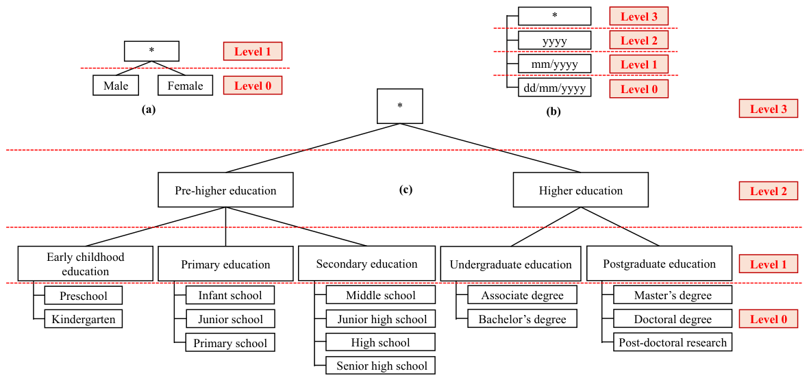
For illustration, consider the Gender, Datetime, and Education attributes of Table 3 as quasi-identifier attributes. A Domain Generalization Hierarchy (DGH) for the Gender attribute, denoted by $DG{H}_{Gender}$, is shown in Figure 1a, which consists of two levels (levels 0 and 1). For the Datetime attribute, a corresponding DGH, denoted by $DG{H}_{Datetime}$, is illustrated in Figure 1b and contains four levels (levels 0, 1, 2, and 3). Similarly, the DGH for the Education attribute, denoted by $DG{H}_{Education}$, is shown in Figure 1c, which also consists of four levels. These DGHs demonstrate that values at lower levels are more specific, whereas values at higher levels are more generalized.

Definition 11

(d-Duplication). Let d be a positive integer, and let $D^{\prime }\left[QI\right]\subseteq D\left[QI\right]$, where $|D^{\prime }\left[QI\right]|\ge d$, denote a specified subset of quasi-identifier tuples in the dataset D. The property of d-Duplication holds if all unique quasi-identifier values of each attribute $q{i}_a$, where $1\le a\le n$, within $D^{\prime }\left[QI\right]$ are either suppressed or generalized using the corresponding values in the Domain Generalization Hierarchy $DG{H}_{D\left[q{i}_a\right]}$, such that they become indistinguishable tuples.

Definition 12

(c-Confidence). Let c be a positive real number. Let $D\left[S\right]$ denote a specified dataset of D, and let $D^{\prime }\left[S\right]$ be a transformed version of $D\left[S\right]$ that satisfies either Definition 5 or Definition 7. The confidence of data re-identification is bounded by the logarithmic measure as $log({\displaystyle \frac{|D^{\prime }\left[S\right]|}{APPE\left(t\right)}})$, where $APPE\left(t\right)$ denotes the number of documents in which the specified term t appears. A larger value of this measure indicates a higher potential risk of re-identification. The dataset $D^{\prime }\left[S\right]$ is said to satisfy the property of c-Confidence if all terms t in $D^{\prime }\left[S\right]$ are suppressed when they satisfy $c>log({\displaystyle \frac{|D^{\prime }\left[S\right]|}{APPE\left(t\right)}})$. This constraint ensures that the confidence of re-identification is bounded by the threshold c, thereby limiting disclosure risk in the released dataset.

Definition 13

(l-Occurence). Let l be a positive integer. Let $D^{\prime }\left[S\right]\subseteq D\left[S\right]$ denote a specified subset of documents in the dataset D. $D^{\prime }\left[S\right]$ can be said to satisfy the property of l-Occurrence when every term t in $D^{\prime }\left[S\right]$ occurs in at least l distinct documents.

2.4. (d, c, l)-Privacy

This section presents three algorithms designed to transform a dataset D so that it satisfies the proposed $(d,c,l)$-Privacy constraints, namely the FCFS, greedy, and optimal $(d,c,l)$-Privacy algorithms. The FCFS $(d,c,l)$-Privacy algorithm primarily focuses on minimizing computational overhead by rapidly transforming D into a sanitized dataset $D^{\prime }$ that conforms to the prescribed privacy constraints. The greedy $(d,c,l)$-Privacy algorithm aims to strike a balance between execution efficiency and data utility preservation in $D^{\prime }$. In contrast, the optimal $(d,c,l)$-Privacy algorithm is designed to maximize the data utility of $D^{\prime }$ while strictly satisfying all privacy requirements. To enforce the $(d,c,l)$-Privacy constraints, let $P=\{p_1,\dots ,p_z\}$ denote a partition of D such that $p_1\cup \dots \cup p_z=D$ and $p_i\cap ,\cdots ,\cap p_j=\varnothing$. Each partition $p_g\in P$ must contain at least d tuples. For each partition $p_g$, every term t in $p_g\left[S\right]$ must satisfy the c-Confidence constraint and occur in at least l distinct documents. In addition, under the term–document measurement mechanism, each term t must have an IDF score within the range $[SWS,c]$. Furthermore, all unique quasi-identifier values in each partition $p_g\left[q{i}_a\right]$, where $1\le g\le z$ and $1\le a\le n$, are either suppressed or generalized to less specific values according to the corresponding Domain Generalization Hierarchy $DG{H}_{D\left[q{i}_a\right]}$, ensuring indistinguishability among tuples within each partition. Data generalization serves as the primary data distortion mechanism in the proposed algorithms, while data suppression is employed as an auxiliary mechanism to eliminate unique tuples and sensitive terms whose IDF scores fall outside the thresholds defined by $SWS$ and c. Accordingly, the penalty cost incurred by generalizing quasi-identifier values across all partitions in P is formalized by Equation (9). A higher value of $GEN(P\left[QI\right],DG{H}_{D\left[q{i}_1\right]},\dots ,DG{H}_{D\left[q{i}_n\right]})$ indicates greater information loss and, consequently, lower data utility.

$$GEN(P\left[QI\right],DG{H}_{D\left[q{i}_1\right]},\dots ,DG{H}_{D\left[q{i}_n\right]})={\displaystyle \sum _{g=1}^z}{\displaystyle \sum _{a=1}^n}{\displaystyle \frac{GEN\_LEVEL\left(p_g\left[q{i}_a\right]\right)}{|DG{H}_{D\left[q{i}_a\right]}|}}$$

(9)

where,

• n represents the total number of quasi-identifier attributes that are available in $P\left[QI\right]$.
• z represents the total number of partitions that are available in $|P|$.
• $GEN\_LEVEL\left(p_g\left[q{i}_a\right]\right)$ represents the level of the generalized value in $q{i}_a$ of $d_x$.
• $|DG{H}_{D\left[q{i}_a\right]}|$ represents the height of the data generalization hierarchy of $DG{H}_{D\left[q{i}_a\right]}$.

In addition to data generalization, P can incur penalty costs associated with suppressing unique tuples and removing unique or uninteresting terms from $D\left[S\right]$. Consequently, two distinct suppression penalty costs are considered. The penalty cost resulting from the suppression of unique tuples is formally defined in Equation (10). The penalty cost associated with suppressing unique or uninteresting terms can be defined in Equation (11). These penalty metrics quantify the loss of data utility introduced by suppression, where higher penalty values indicate greater information loss and, therefore, lower data utility.

$$SU{P}_1(D,P)=1-{\displaystyle \frac{|D|-{\sum }_{g=1}^z|P\left[p_g\right]|}{|D|}},where{\displaystyle \sum _{g=1}^z}|P\left[p_g\right]|=|D^{\prime }|$$

(10)

$$SU{P}_2(D,P)=1-{\displaystyle \frac{{\sum }_{x=1}^m|D\left[d_x\left[S\right]\right]|-{\sum }_{g=1}^z|P\left[p_g\left[d_x\left[S\right]\right]\right]|}{{\sum }_{x=1}^m|D\left[d_x\left[S\right]\right]|}}$$

(11)

where,

• $|D[d_x\left[S\right]]|$ is the total number of the terms t in $D\left[d_x\left[S\right]\right]$.
• $|P[p_g\left[d_x\left[S\right]\right]]|$ is the total number of the terms t in $P\left[p_g\left[d_x\left[S\right]\right]\right]$.

Accordingly, the total penalty cost of the partition set P can be defined by Equation (12). Specifically, this total penalty cost is determined by the combined effects of the penalty incurred from generalizing quasi-identifier values and the penalty incurred from suppressing unique tuples and terms.

$$\begin{array}{cc}\hfill PEN(D,P)& =GEN(P\left[QI\right],DG{H}_{D\left[q{i}_1\right]},\dots ,DG{H}_{D\left[q{i}_n\right]})+SU{P}_1(D,P)+SU{P}_2(D,P)\hfill \end{array}$$

(12)

$$\begin{array}{cc}\hfill O_1(DATA\_PREP(D,T,SWS,c))& =(|D\left[S\right]|·O(ALG\_ETF(T,D\left[d_x\left[S\right]\right])))\hfill \\ & +(2·O(ALG\_EIDF(T,D[S\left]\right)\left)\right)\hfill \end{array}$$

(13)

$$\begin{array}{c}\hfill O_2(DATA\_PREP(D,T,SWS,c))=2·O(ALG\_TFIDF(T,D\left[S\right]))\end{array}$$

(14)

2.4.1. FCFS (d, c, l)-Privacy Algorithm

This section introduces a heuristic algorithm that is designed to transform the dataset D into a sanitized version $D^{\prime }$ that satisfies the proposed $(d,c,l)$-Privacy constraints. The algorithm follows a First-Come-First-Served (FCFS) strategy and is referred to as the FCFS $(d,c,l)$-Privacy algorithm. In addition to ensuring compliance with the $(d,c,l)$-Privacy requirements, this algorithm primarily emphasizes minimizing execution time, thereby enabling an efficient data transformation process. The data preparation steps are described in Algorithm 6, which prepares the dataset before it is processed by the FCFS heuristic algorithm presented in Algorithm 7.

Algorithm 7 takes as input the dataset D, the Domain Generalization Hierarchies $DG{H}_{D\left[q{i}_1\right]},\dots ,DG{H}_{D\left[q{i}_n\right]}$, the expert term set T, the stopword threshold $SWS$, and the privacy parameters d, c, and l. The output of the algorithm is a sanitized dataset $D^{\prime }$ that satisfies the specified $(d,c,l)$-Privacy constraints.

To transform D into $D^{\prime }$, the algorithm first executes a set of data preparation processes that are described in Algorithm 6. Under the expert term document measurement, any term t whose EIDF score is greater than c is to be suppressed. In contrast, under the mechanism term document measurement, a term t is suppressed if its IDF score is greater than c or lower than $SWS$. Algorithm 6 first checks whether the expert term set T is non-empty. When $T\ne \varnothing$, the expert-based preparation process is activated. Specifically, ETF and EIDF scores are computed for each term t in D (lines 2–12). The computational complexity of this process is formally expressed in Equation (13). When $T=\varnothing$, the mechanism-based preparation process is executed (lines 14–20). In this case, the tuples of D, together with their TF, IDF, and TFIDF scores, are stored in a temporary dataset $TP2:=D\left[QI\right]\cup TP1\left[S\right]\cup TP1\left[TF\right]\cup TP1\left[IDF\right]\cup TP1\left[TFIDF\right]$. The dataset $TP2$ is then iterated, and any term t with an IDF score greater than c and an IDF score lower than $SWS$ is suppressed. The computational complexity of this process is shown in Equation (14).

Algorithm 6 DATA_PREP(D, T, SWS, c)

Require: $D,T,SWS,c$ Ensure: $D^{\prime }$   1: $D^{\prime }:=\varnothing ,TP1:=\varnothing ,TP2:=\varnothing ,TP3:=\varnothing$   2: if $T\ne \varnothing$ then   3:     for $x:=1to|D[S]|$ do   4:         $TP1:=TP1\cup ALG\_ETF(T,D\left[d_x\left[S\right]\right]))$   5:     end for   6:     $TP2:=ALG\_EIDF(T,D[S\left]\right)$   7:     $TP3:=D\left[QI\right]\cup \left(TP1\right[S]\vee TP2[S\left]\right)\cup TP1\left[ETF\right]\cup TP2\left[EIDF\right]$   8:     for $x:=1to|TP3|$ do   9:         if $TP3\left[EIDF\right]\le c$ then 10:            $D^{\prime }:=D^{\prime }\cup TP3\left[d_x\right]$ 11:         end if 12:     end for 13: else 14:     $TP1:=ALG\_TFIDF(T,D[S\left]\right)$ 15:     $TP2:=D\left[QI\right]\cup TP1\left[S\right]\cup TP1\left[TF\right]\cup TP1\left[IDF\right]\cup TP1\left[TFIDF\right]$ 16:     for $x:=1to|TP2|$ do 17:         if $TP2\left[IDF\right]\ge SWSandTP2\left[IDF\right]\le c$ then 18:            $D^{\prime }:=D^{\prime }\cup TP2\left[d_x\right]$ 19:         end if 20:     end for 21: end if 22: Return $D^{\prime }$

$$\begin{array}{c}\hfill O\left(FCFS\right)=2·O(DATA\_PREP(D,T,SWS,c))+(m·n·|DG{H}_{D\left[q{i}_a\right]}|)\end{array}$$

(15)

After the data preparation processes are completed, Algorithm 7 proceeds to partition the remaining tuples. The algorithm first checks whether $TP1$ can satisfy the values of d and l. If not, the algorithm terminates and returns $Failure$. Otherwise, tuples are iteratively assigned to temporary partitions following a First-Come-First-Served (FCFS) strategy. If the size of $TP1$ is less than $2·d$ or the number of distinct terms in $\Lambda \left[S\right]$ is less than $2cotl$, the remaining tuples are merged into a single partition. The quasi-identifier values $TP1\left[QI\right]$ are then suppressed or generalized using the corresponding hierarchies $DG{H}_{D\left[q{i}_1\right]},\dots ,DG{H}_{D\left[q{i}_n\right]}$ to ensure indistinguishability. Otherwise, tuples are incrementally selected from $TP1$ and inserted into a temporary partition until the d-Duplication and l-Occurrence constraints are satisfied. Once these conditions hold, the temporary partition is finalized as a partition of $D^{\prime }$, and the process repeats until all tuples are allocated. Under the expert term document measurement, the ETF and EIDF scores are stored within each partition. Under the mechanism-based measurement, TF and IDF scores are stored instead, and further collect the TFIDF score of each term t. Due to its FCFS strategy, the order of tuples determines the resulting partitions, enabling efficient execution while enforcing all $(d,c,l)$-Privacy constraints. Finally, the algorithm returns $D^{\prime }$ that is satisfied by $(d,c,l)$-Privacy constraints.

The overall computational complexity of the FCFS heuristic algorithm is formally derived in Equation (15).  

Algorithm 7 FCFS $(d,c,l)$-Privacy algorithm

Require: $D,DG{H}_{D\left[q{i}_1\right]},\dots ,DG{H}_{D\left[q{i}_n\right]},T,SWS,d,c,l$ Ensure: $D^{\prime }$   1: $D^{\prime }:=\varnothing ,TP1:=\varnothing ,TP2:=\varnothing ,p:=\varnothing$   2: $TP1:=DATA\_PREP(D,T,SWS,c)$   3: if $|TP1|<dorDISTINCT\_COUNT\left(TP1\right[S\left]\right)<l$ then   4:     Return $Failure$   5: else   6:     while $TP1$ do   7:         if $(|TP1|<2·dorDISTINCT\_COUNT(TP1\left[S\right])<2·l)andp=\varnothing$ then   8:            $TP2:=DISTORT((TP1\left[QI\right],DG{H}_{D\left[q{i}_1\right]},\dots ,DG{H}_{D\left[q{i}_n\right]})$   9:            if $T\ne \varnothing$ then 10:                $D^{\prime }:=D^{\prime }\cup (TP2\cup TP1\left[t\right]\cup TP1\left[TF\right]\cup TP1\left[IDF\right])$ 11:            else 12:                $D^{\prime }:=D^{\prime }\cup (TP2\cup TP1\left[t\right]\cup TP1\left[TF\right]\cup TP1\left[IDF\right]\cup TP1\left[TFIDF\right])$ 13:            end if 14:            $TP1:=\varnothing$ 15:         else 16:            $p:=p\cup TP1\left[d_x\right]$ 17:            if $|p|\ge dorDISTINCT\_COUNT\left(p\right[S\left]\right)\ge l$ then 18:                $TP2:=DISTORT(p\left[QI\right],DG{H}_{D\left[q{i}_1\right]},\dots ,DG{H}_{D\left[q{i}_n\right]})$ 19:                if $T\ne \varnothing$ then 20:                    $D^{\prime }:=D^{\prime }\cup (TP2\cup p\left[t\right]\cup p\left[TF\right]\cup p\left[IDF\right]$ 21:                else 22:                    $D^{\prime }:=D^{\prime }\cup (TP2\cup p\left[t\right]\cup p\left[TF\right]\cup p\left[IDF\right]\cup p\left[TFIDF\right])$ 23:                end if 24:                $p:=\varnothing$ 25:            else 26:                $TP1:=TP1-TP1\left[d_x\right]$ 27:            end if 28:         end if 29:     end while 30: end if 31: Return $D^{\prime }$

Theorem 1.

If $D^{\prime }$ satisfies the $(d,c,l)$-Privacy constraints, then it ensures that: (i) the data utilization for each term $t\in D^{\prime }\left[S\right]$ includes at least d satisfied tuples; (ii) the confidence of data re-identification for each term $t\in D^{\prime }\left[S\right]$ is at most c; and (iii) the number of distinct terms $t\in D^{\prime }\left[S\right]$ is at least l.

Proof. 

Assume that $D^{\prime }$ satisfies $(d,c,l)$-Privacy. We prove each claim by contradiction.

(i)

The data utilization for each term $t\in D^{\prime }\left[S\right]$ includes at least d satisfied tuples.

Assume, for contradiction, that there exists a term $t\in D^{\prime }\left[S\right]$ whose data utilization contains fewer than d satisfied tuples, i.e., $|\{\tau \in D^{\prime }\mid \tau \left[S\right]=t\}|<d$. However, by the definition of $(d,c,l)$-Privacy, every released term must be supported by at least d tuples. This contradicts the assumption that $D^{\prime }$ satisfies the d-constraint. Therefore, the data utilization of each term $t\in D^{\prime }\left[S\right]$ contains at least d satisfied tuples.

(ii)

The confidence of data re-identification for each term $t\in D^{\prime }\left[S\right]$ is at most c.

Assume, for contradiction, that there exists a term $t\in D^{\prime }\left[S\right]$ whose confidence of data re-identification is greater than c. The $(d,c,l)$-Privacy model enforces an upper bound c on the maximum re-identification confidence for any sensitive term. Hence, such a term violates the c-constraint, contradicting the assumption that $D^{\prime }$ satisfies $(d,c,l)$-Privacy. Therefore, the confidence of data re-identification for each term $t\in D^{\prime }\left[S\right]$ does not exceed c.

(iii)

The number of distinct terms $t\in D^{\prime }\left[S\right]$ is at least l.

Assume, for contradiction, that the number of distinct terms in $D^{\prime }\left[S\right]$ exceeds l, i.e., $|D^{\prime }\left[S\right]|>l$. The definition of $(d,c,l)$-Privacy restricts the number of distinct sensitive terms to at most l. This assumption contradicts the l-constraint. Hence, the number of distinct terms $t\in D^{\prime }\left[S\right]$ does not exceed l.

Since each contradiction violates the definition of $(d,c,l)$-Privacy, all three properties must hold.    □

2.4.2. Greedy (d, c, l)-Privacy

In this section, a greedy $(d,c,l)$-Privacy model based on a local optimization strategy is proposed. The objective of this algorithm is to transform datasets to satisfy the $(d,c,l)$-Privacy constraints. The transformation process and the characteristics of the resulting datasets differ from those of the algorithms presented in Section 2.4.1 and Section 2.4.3.

The proposed algorithm is designed to address privacy violations in datasets while preserving data utility and minimizing the execution time of the data transformation. The complete procedure of the algorithm is presented in Algorithm 8. The inputs to the algorithm include the original dataset D, the domain generalization hierarchies $DG{H}_{D\left[q{i}_1\right]},\dots ,DG{H}_{D\left[q{i}_n\right]}$, T, $SWS$, and the privacy parameters d, c, and l.

$$\begin{array}{cc}\hfill O\left(Greedy\right)& =O(DATA\_PREP(D,T,SWS,c))+(m^2·n·|DG{H}_{D\left[q{i}_a\right]}|+\hfill \\ & (g·(d-1)·|DG{H}_{D\left[q{i}_a\right]}|\hfill \end{array}$$

(16)

With Algorithm 8, before the tuples of the temporary dataset $TP1$ are partitioned, they are first validated to ensure compliance with the given value of d and l. This data validation process is implemented in the lines between 3 and 5 of the algorithm. If it is not satisfied by the given value of d and l, the algorithm terminates and returns $Failure$. Otherwise, the tuples of the temporary dataset are assigned to their appropriate partition. To achieve the algorithm’s objective of assigning tuples to their appropriate partitions, the size of $TP1$ is first investigated if the size of $TP1$ does not exceed $d·2$ and the number of distinct terms t in $TP1\left[S\right]$ does not exceed $l·2$ then the tuples of $TP1$ can only be constructed to be one partition of $D^{\prime }$. Thus, the unique values in each quasi-identifier attribute of $TP1$ are suppressed or generalized by their less specific values, and they are inserted into $D^{\prime }$. This data process is implemented in the lines between 6 and 12 of the algorithm. If not, all tuples are available in $TP1$ to be iterated. During the iteration, an arbitrary tuple $d_x\in TP1$ (i.e., $TP1\left[d_x\right]$) is selected to the initial tuple of the specifically constructed partition, i.e., $TP2:=TP1\left[d_x\right]$. The remaining tuples are stored in $TP3$, i.e., $TP3:=TP1-TP2$. Subsequently, a tuple $d_x\in TP3$ (i.e., $TP3\left[d_x\right]$) is the closeness tuple of $TP3\left[d_x\right]$ is selected until the constraints specified in d and l are satisfied. In addition, the closeness tuple $TP3\left[d_x\right]$ of $TP1\left[d_x\right]$ is an arbitrary tuple in $TP3$ such that the combined result of them is the lowest penalty cost of data generalization. The procedure for selecting the closeness tuple is implemented in the lines between 17 and 20 of the algorithm. If the tuples of $TP2$ satisfy the given values of d and l, they are constructed into a partition of $D^{\prime }$. The process of constructing partitions is implemented in the lines between 21 and 33. That is, the unique quasi-identifier values of $TP2$ (i.e., $TP2\left[QI\right]$) are suppressed or generalized by their less specific values that are available in $DG{H}_{D\left[q{i}_1\right]},\dots ,DG{H}_{D\left[q{i}_n\right]}$ to be indistinguishable; this data processing is implemented in the line 26, i.e., $TP:=DISTORT(TP2\left[QI\right],DG{H}_{D\left[q{i}_1\right]},\dots ,DG{H}_{D\left[q{i}_n\right]})$. Moreover, an arbitrary tuple is selected to be the initial tuple for constructing the next partition of $D^{\prime }$, i.e., $TP2:=TP1\left[d_x\right]$. In addition, in each iteration, the considered tuple is removed from the temporary dataset, i.e., $TP3:=TP3-TP3\left[d_x\right]$. The construction of partitions in $D^{\prime }$ proceeds until either the size of the temporary dataset falls below d or the number of distinct values in the temporary dataset falls below l. Once either condition is met, the process of constructing new partitions of $D^{\prime }$ is terminated. All remaining tuples in the temporary dataset are then inserted into an arbitrarily chosen appropriate partition of $D^{\prime }$. This procedure is repeated until the temporary dataset becomes empty. The implementation of this process is implemented in the lines between 36 and 52 of the algorithm. Finally, the algorithm returns $D^{\prime }$ that is satisfied by $(d,c,l)$-Privacy constraints. Consequently, the computational complexity of Algorithm 8 can be presented by in Equation (16).

Theorem 2.

Let $ST\subseteq D$ be a set of tuples that are the most similar to a given tuple $d_x$ under the distance measure $DIST(·,·)$. Then, the partition $ST\cup d_x$ incurs the minimum possible penalty cost of data generalization among all partitions of the same size containing $d_x$.

Proof. 

Assume that the penalty cost of data generalization is defined as the sum of the heights of the least common ancestors (LCAs) in the corresponding domain generalization hierarchies $DG{H}_{D\left[q{i}_1\right]},\dots ,DG{H}_{D\left[q{i}_n\right]}$ over all quasi-identifier attributes. Let $p_x=ST\cup d_x$ be the partition formed by the tuples that are most similar to $d_x$. By construction, for every tuple $d_y\in ST$ and for every quasi-identifier attribute $q{i}_a$, we have $DIS{T}_a(d_y,d_x)\le DIS{T}_a(d_z,d_x)$, for any tuple $d_z\in D\setminus ST$. Suppose, for the sake of contradiction, that there exists another partition $p_x^{\prime }=S{T}^{\prime }\cup D\left[d_x\right]$, where $|S{T}^{\prime }|=|ST|$, such that the penalty cost of data generalization of $p_x^{\prime }$ is strictly smaller than that of $p_x$. Then, $S{T}^{\prime }$ must contain at least one tuple $d_z\notin ST$. Since $ST$ consists of the most similar tuples to $d_x$, there exists at least one attribute $q{i}_a$ for which $DIS{T}_a(d_z,d_x)>{max}_{d_y\in ST}DIS{T}_a(d_y,d_x)$. Consequently, the least common ancestor induced by the set $\{d_z,d_x\}$ in the hierarchy $DG{H}_{D\left[q{i}_a\right]}$ must be located at the same level or higher than the LCA induced by $\{d_y,d_x\}$ for any $d_y\in ST$. Therefore, the LCA height for attribute $q{i}_a$ in $p_x^{\prime }$ is greater than or equal to that in $p_x$. Since the total penalty cost is a nonnegative sum of LCA heights across all quasi-identifier attributes, a weak increase in at least one attribute implies that the overall penalty cost of $p_x^{\prime }$ cannot be smaller than that of $p_x$. This contradicts the assumption that $p_x^{\prime }$ has a strictly lower penalty cost than $p_x$. Hence, no such partition $p_x^{\prime }$ exists, and the partition $ST\cup d_x$ achieves the minimum possible penalty cost of data generalization.    □

2.4.3. Optimal (d, c, l)-Privacy

In this section, another algorithm is proposed to transform the original dataset D into $D^{\prime }$ such that $D^{\prime }$ satisfies $(d,c,l)$-Privacy constraints. The primary objective of this algorithm is not only to ensure compliance with the $(d,c,l)$-Privacy requirements but also to preserve the data utility of $D^{\prime }$ as much as possible. This algorithm is referred to be optimal $(d,c,l)$-Privacy algorithm, and its detailed procedure is presented in Algorithm 9. The input parameters of the algorithm include the original dataset D, the domain generalization hierarchies $DG{H}_{D\left[q{i}_1\right]},\dots ,DG{H}_{D\left[q{i}_n\right]}$, T, $SWS$, and the privacy parameters d, c, and l. Furthermore, before the transformation process is applied to enforce the $(d,c,l)$-Privacy constraints, the dataset must undergo a preprocessing step using Algorithm 6.

With Algorithm 9, the first step is to validate the temporary dataset $TP1$ to ensure that it can be transformed in accordance with the specified values of d and l. If $TP1$ fails to satisfy either the d-constraint or the l-constraint, the algorithm terminates and returns Failure. Otherwise, subsequent processing steps are enabled, during which each tuple in $TP1$ is assigned to an appropriate partition. To achieve the objective of partitioning tuples effectively, both the size of $TP1$ and the number of distinct terms t in $TP1\left[S\right]$ are examined. Specifically, if the cardinality of $TP1$ does not exceed $2d$ or the number of distinct terms in $TP1\left[S\right]$ does not exceed $2l$, then all tuples in $TP1$ are constructed as a single partition of $D^{\prime }$. In this case, the distinct quasi-identifier values in $TP1$ are suppressed or generalized to less specific values to ensure indistinguishability. If neither condition is satisfied, all possible partitions of $D^{\prime }$ that meet the given d- and l-constraints are constructed using a nested-loop procedure. Furthermore, the candidate data versions $D^{\prime }$ are generated from sets of partitions $\{p_{g_1},\dots ,p_{g_{|P|-1}}\}$ that satisfy $p_{g_1}\cap \cdots \cap p_{g_{|P|-1}}=\varnothing$ and $p_{g_1}\cup \dots \cup p_{g_{|P|-1}}=D$, ensuring that the partitions are both disjoint and collectively exhaustive with respect to the original dataset D. Among all valid candidate versions, the final released dataset $D^{\prime }$ is selected as the one with the lowest penalty cost associated with data suppression and generalization. Finally, the algorithm returns $D^{\prime }$ that is satisfied by $(d,c,l)$-Privacy constraints. Consequently, the computational complexity of Algorithm 9 is presented in Equation (17).

$$\begin{array}{c}\hfill O\left(Optimal\right)={\displaystyle \sum _{P\_SIZE:=m-d}^m}P\_SIZE·C(m,P\_SIZE)+(2^{|P|}·(n·|DG{H}_{D\left[q{i}_a\right]}|))\end{array}$$

(17)

where,

• $P\_SIZE$ is the size of the constructed partitions.
• $C(m,P\_SIZE)$ is the total number of $P\_SIZE$ partitions that are constructed from m tuples of D.
• $|P|$ is the total number of the constructed partitions.

Theorem 3.

If $D^{\prime }$ is a suppressed and generalized version of D that achieves the highest possible data utility under the $(d,c,l)$-Privacy constraints, then every partition (equivalence class) of $D^{\prime }$ incurs the minimum possible penalty cost associated with data suppression and generalization.

Proof. 

Assume that data utility is inversely related to the penalty cost of data suppression and generalization, such that lower penalty costs correspond to higher data utility. Furthermore, assume that the total penalty cost of $D^{\prime }$ is computed as the sum of the penalty costs incurred by all its partitions. Suppose, for the sake of contradiction, that $D^{\prime }$ achieves the highest possible data utility, but there exists at least one partition $p_x\subseteq D^{\prime }$ whose penalty cost is not minimal. Then there must exist an alternative partition $p_x^{\prime }$ defined over the same set of original tuples that satisfies the $(d,c,l)$-Privacy constraints and incurs a strictly lower penalty cost than p. By replacing $p_x$ with $p_x^{\prime }$, the overall penalty cost of $D^{\prime }$ would be strictly reduced while preserving compliance with the privacy constraints. Since a lower penalty cost implies higher data utility, the resulting dataset would have strictly greater data utility than $D^{\prime }$. This contradicts the assumption that $D^{\prime }$ already achieves the highest possible data utility. Therefore, no such partition $p_x$ can exist, and it follows that every partition of $D^{\prime }$ must incur the minimum possible penalty cost of data suppression and generalization.    □

Algorithm 8 Greedy $(d,c,l)$-Privacy algorithm

Require: $D,T,STW,DG{H}_{D\left[q{i}_1\right]},\dots ,DG{H}_{D\left[q{i}_n\right]},d,c,l$ Ensure: $D^{\prime }$   1: $TP1:=\varnothing ,TP2:=\varnothing ,TP3:=\varnothing ,TP4:=\varnothing ,TP5=\varnothing ,P:=\varnothing ,ST:\varnothing ,SS\leftarrow 0,GS\leftarrow \infty$   2: $TP1:=DATA\_PREP(D,T,SWS,c)$   3: if $|TP1|<dorDISTINCT\_COUNT\left(TP1\right[S\left]\right)<l$ then   4:     Return $Failure$   5: else   6:     if $|TP1|<d·2orDISTINCT\_COUNT\left(TP1\right[S\left]\right)<l·2$ then   7:         $TP3:=DISTORT(TP1,\left[QI\right],DG{H}_{D\left[q{i}_1\right]},\dots ,DG{H}_{D\left[q{i}_n\right]})$   8:         if $T\ne \varnothing$ then   9:            $D^{\prime }:=TP3\cup |TP1|\cup TP1\left[t\right]\cup TP1\left[TF\right]\cup TP1\left[IDF\right]$ 10:         else 11:            $D^{\prime }:=TP3\cup |TP1|\cup TP1\left[t\right]\cup TP1\left[TF\right]\cup TP1\left[IDF\right]\cup TP1\left[TFIDF\right]$ 12:         end if 13:     else 14:         $TP2:=TP1\left[d_x\right]$, $TP3:=TP1-TP2$, $TP1:=TP1-TP2$, $TP4:=\varnothing$, $ST:=\varnothing$, $SS:=0$, $GS:=\infty$ 15:         while $TP3$ do 16:            $SS:=DISTORT(TP2\left[QI\right]\cup TP3\left[d_x\left[QI\right]\right],DG{H}_{D\left[q{i}_1\right]},\dots ,DG{H}_{D\left[q{i}_n\right]})$ 17:            if $GS>SS$ then 18:                $ST:=TP3\left[d_x\right]$ 19:                $GS:=SS$ 20:            end if 21:            $TP3:=TP3-TP3\left[d_x\right]$ 22:            if $|TP3|=0$ then, i.e., $TP3:=\varnothing$ 23:                $TP2:=TP2\cup ST$ 24:                $TP3:=TP1-ST$ 25:                if $|TP2|>=dandDISTINCT\_COUNT\left(TP2\right[S\left]\right)>=l$ then 26:                    $TP4:=DISTORT(TP2\left[QI\right],DG{H}_{D\left[q{i}_1\right]},\dots ,DG{H}_{D\left[q{i}_n\right]})$ 27:                    if $T\ne \varnothing$ then 28:                        $P:=P\cup (TP4\cup TP2[t]\cup TP2[TF]\cup TP2[IDF]$ 29:                    else 30:                        $P:=P\cup (TP4\cup TP2[t]\cup TP2[TF]\cup TP2[IDF]\cup TP2[TFIDF\left]\right)$ 31:                    end if 32:                    $TP2:=TP1\left[d_x\right]$, $SS:=0$, $GS:=\infty$, $ST:=\varnothing$, $TP3:=TP1-TP1\left[d_x\right]$ 33:                end if 34:                $TP1:=TP3$ 35:            end if 36:            if $(|TP1|<dand|TP1|>0)orDISTINCT\_COUNT\left(TP1\right[S\left]\right)<l$ then 37:                for $g:=1to|P|$ do 38:                    $SS:=DISTORT(p_g\left[QI\right]\cup TP1\left[d_x\left[QI\right]\right],DG{H}_{D\left[q{i}_1\right]},\dots ,DG{H}_{D\left[q{i}_n\right]})$ 39:                    if $GS>SS$ then 40:                        $ST:=p_g$ 41:                        $GS:=SS$ 42:                    end if 43:                end for 44:                ${\rm Y}:=ST\cup TP1\left[d_x\right]$ 45:                $P:=P-ST$ 46:                $TP4:=DISTORT(TP5\left[QI\right],DG{H}_{D\left[q{i}_1\right]},\dots ,DG{H}_{D\left[q{i}_n\right]})$ 47:                if $T\ne \varnothing$ then 48:                    $P:=P\cup (TP4\cup TP5[t]\cup TP5[TF]\cup TP5[IDF]$ 49:                else 50:                    $P:=P\cup (TP4\cup TP5[t]\cup TP5[TF]\cup TP5[IDF]\cup TP5[TFIDF\left]\right)$ 51:                end if 52:                $TP1:=TP1-TP1\left[d_x\right]$, $SS:=0$, $GS:=\infty$ 53:            end if 54:         end while 55:     end if 56:     $D^{\prime }=P$ 57: end if 58: Return $D^{\prime }$

Algorithm 9 Optimal $(d,c,l)$-Privacy algorithm

Require: $D,T,STW,DG{H}_{D\left[q{i}_1\right]},\dots ,DG{H}_{D\left[q{i}_n\right]},d,c,l$   1: $TP1:=\varnothing ,TP2:=\varnothing ,TP3:=\varnothing ,P:=\varnothing ,V:=\varnothing ,SP:=0,GP:=\infty$   2: $TP1:=DATA\_PREP(D,T,SWS,c)$   3: if $|TP1|<dor|TP1[S]|<corDISTINCT\_COUNT\left(TP1\right[S\left]\right)<l$ then   4:     Return $Failure$   5: else   6:     if $|TP1|<d·2orDISTINCT\_COUNT\left(TP1\right[S\left]\right)<l·2$ then   7:         $TP2:=DISTORT(TP1\left[QI\right],DG{H}_{D\left[q{i}_1\right]},\dots ,DG{H}_{D\left[q{i}_n\right]})$   8:         if $T\ne \varnothing$ then   9:            $D^{\prime }:=TP2\cup |TP1|\cup TP1\left[t\right]\cup TP1\left[TF\right]\cup TP1\left[IDF\right]$ 10:         else 11:            $D^{\prime }:=TP2\cup |TP1|\cup TP1\left[t\right]\cup TP1\left[TF\right]\cup TP1\left[IDF\right]\cup TP1\left[TFIDF\right]$ 12:         end if 13:     else 14:         for $P\_SIZE:=dto|TP1|$ do 15:            for $x_{m-P\_SIZE+1}:=1tom-P\_SIZE+1$ do 16:                . 17:                . 18:                . 19:                for $x_{m-1}:=x_{m-2}+1tom-1$ do 20:                    for $x_{m-0}:=x_{m-1}+1tom-0$ do 21:                        $P:=P\cup (d_{x_{m-P\_SIZE+1}}\cup \dots cup{d}_{x_{m-1}}\cup d_{x_{m-0}})$ 22:                    end for 23:                end for 24:            end for 25:         end for 26:         for $g_1:=1to|P|$ do 27:            . 28:            . 29:            . 30:            for $g_{|P|-2}:=|P|-2to|P|$ do 31:                for $g_{|P|-1}:=|P|-1to|P|$ do 32:                    if $p_{g_1}\cap \cdots \cap p_{g_{|P|-2}}\cap p_{g_{|P|-1}}=\varnothing and{p}_{g_1}\cup \dots \cup p_{g_{|P|-2}}\cup p_{g_{|P|-1}}=D$ then 33:                        $TP3:=p_{g_1}\cup \dots \cup p_{g_{|P|-2}}\cup p_{g_{|P|-1}}$ 34:                        $SP:=DISTORT(TP3\left[QI\right],DG{H}_{D\left[q{i}_1\right]},\dots ,DG{H}_{D\left[q{i}_n\right]})$ 35:                        if $GP>SP$ then 36:                           $TP2:=SP$ 37:                           if $T\ne \varnothing$ then 38:                               $D^{\prime }:=D^{\prime }\cup (TP2\cup TP1\left[t\right]\cup TP1\left[TF\right]\cup TP1\left[IDF\right]$ 39:                           else 40:                               $D^{\prime }:=D^{\prime }\cup (TP2\cup TP1\left[t\right]\cup TP1\left[TF\right]\cup TP1\left[IDF\right]\cup TP1\left[TFIDF\right])$ 41:                           end if 42:                           $GP:=SP$ 43:                        end if 44:                    end if 45:                end for 46:            end for 47:         end for 48:     end if 49: end if 50: Return $D^{\prime }$

2.4.4. Hardness

In this section, we illustrate that the optimal $(d,c,l)$-Privacy algorithm is NP-hard [57] by providing a reduction from the Exact Cover by 3-Sets problem (X3C) [58]. At first, we formally introduce the X3C problem as follows.

Exact Cover by 3-Sets problem ($\mathit{X}\mathbf{3}\mathit{C}$): Let U be a universal set with cardinality $|U|=3q$, where $q\in {\mathbb{Z}}^{+}$. Define $S=\{s\subseteq U\mid |s|=3\}$ as the collection of all 3-element subsets of U. The Exact Cover by 3-Sets ($X3C$) problem asks whether there exists a subcollection $S^{\prime }\subseteq S$ such that:

• Every element $u_i\in U$ appears in exactly one subset of $S^{\prime }$.
• The union of all subsets in S’ covers the entire universe, i.e., ${\cup }_{s^{\prime }\in S^{\prime }}{s}^{\prime }=U$.
• The subsets in S’ are pairwise disjoint, i.e., ${\cap }_{s^{\prime }\in S^{\prime }}{s}^{\prime }=\varnothing$.

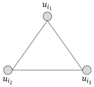
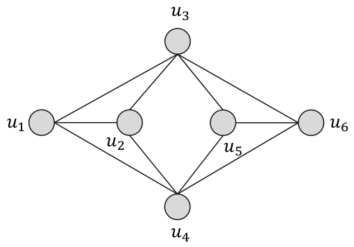
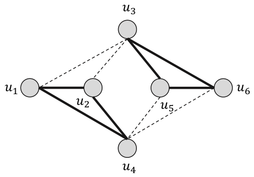
The $X3C$ problem can be naturally represented using graph-theoretic notation. Let V be the set of vertices corresponding to the elements of U. Let E be the set of edges, where each edge represents the relationship between any pair of elements contained in a subset $s\in S$. Thus, the graph $G=(V,E)$ serves as a representation of the $X3C$ instance. By construction, G is a simple undirected graph, meaning that loops and multiple edges are disallowed. Furthermore, each subset $s\in S$ can be represented as a complete graph on three vertices, $K_3$, as illustrated in Figure 2. For example, consider the instance where $U=\{u_1,$$u_2,$$u_3,$$u_4,$$u_5,$$u_6\}$ and $S=\left\{\right\{u_1,$$u_2,$$u_3\},$$\{u_1,$$u_2,$$u_4\},$$\{u_3,$$u_5,$$u_6\},$$\{u_4,$$u_5,$$u_6\left\}\right\}$. The corresponding $X3C$ graph constructed from this instance is shown in Figure 3.

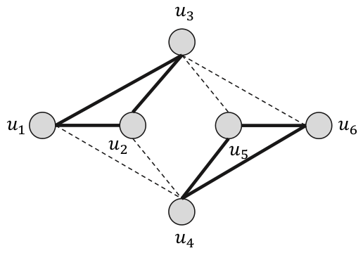
To solve the $X3C$ problem, the subcollection $S^{\prime }$ can be constructed directly from the $X3C$ graph. Specifically, $S^{\prime }$ corresponds to a set of arbitrary 3-vertex subgraphs that are complete, pairwise disjoint, and collectively cover all elements of U. From the input instance illustrated in Figure 3, there exist two valid solutions $S^{\prime }$ that satisfy the $X3C$ constraints:

• $S_1^{\prime }$=$\left\{\right\{u_1,$$u_2,$$u_3\},$$\{u_4,$$u_5,$$u_6\left\}\right\}$
• $S_2^{\prime }$=$\left\{\right\{u_1,$$u_2,$$u_4\},$$\{u_3,$$u_5,$$u_6\left\}\right\}$

These solutions are depicted in Figure 4 and Figure 5, respectively.

We now illustrate that optimal $(d,c,l)$-Privacy algorithm is NP-hard by constructing a reduction from the $X3C$ problem. For clarity, we restrict our consideration to quasi-identifier attributes in both datasets, i.e., D and $D^{\prime }$. The dataset D is constructed from the universe U and the collection S. Suppose the size of D is $3q·3q$, and the parameter d (d-Duplication) is set to 3. For each arbitrary edge $(u_i,u_j)\in E$, we associate the cells $D\left[d_i\left[q{i}_i\right]\right],D\left[d_j\left[q{i}_j\right]\right],D\left[d_i\left[q{i}_j\right]\right],$ and $D\left[d_j\left[q{i}_i\right]\right]$ of D with the value 1, while all other cells are assigned the value 0. As an example, consider the $X3C$ graph with $q=2$ shown in Figure 3. This graph can be represented as an instance of the specified dataset, as illustrated in

Table 14. The dataset D, which it is constructed from the graph in Figure 3.

	${\mathit{u}}_1$	${\mathit{u}}_2$	${\mathit{u}}_3$	${\mathit{u}}_4$	${\mathit{u}}_5$	${\mathit{u}}_6$
${\mathit{u}}_{\mathbf{1}}$	1	1	1	1	0	0
${\mathit{u}}_{\mathbf{2}}$	1	1	1	1	0	0
${\mathit{u}}_{\mathbf{3}}$	1	1	1	0	1	1
${\mathit{u}}_{\mathbf{4}}$	1	1	0	1	1	1
${\mathit{u}}_{\mathbf{5}}$	0	0	1	1	1	1
${\mathit{u}}_{\mathbf{6}}$	0	0	1	1	1	1

. Subsequently, the dataset $D^{\prime }$ of D can be constructed from the solution graphs $S^{\prime }$ of the $X3C$ problem. Specifically,

Table 15. The dataset $D_1^{\prime }$ satisfied by d-Duplication with $d=3$, constructed from the graph in Figure 4.

	${\mathit{u}}_1$	${\mathit{u}}_2$	${\mathit{u}}_3$	${\mathit{u}}_4$	${\mathit{u}}_5$	${\mathit{u}}_6$
$u_1$	1	1	1	0	0	0
$u_2$	1	1	1	0	0	0
$u_3$	1	1	1	0	0	0
$u_4$	0	0	0	1	1	1
$u_5$	0	0	0	1	1	1
$u_6$	0	0	0	1	1	1

and

Table 16. The dataset $D_2^{\prime }$ satisfied by d-Duplication with $d=3$, constructed from the graph in Figure 5.

	${\mathit{u}}_1$	${\mathit{u}}_2$	${\mathit{u}}_3$	${\mathit{u}}_4$	${\mathit{u}}_5$	${\mathit{u}}_6$
$u_1$	1	1	0	1	0	0
$u_2$	1	1	0	1	0	0
$u_3$	0	0	1	0	1	1
$u_4$	1	1	0	1	0	0
$u_5$	0	0	1	0	1	1
$u_6$	0	0	1	0	1	1

correspond to $D_1^{\prime }$ and $D_2^{\prime }$, which are derived from the solution graphs $S_1^{\prime }$ in Figure 4 and $S_2^{\prime }$ in Figure 5, respectively.

Theorem 4.

The privacy preservation for datasets which is based on the optimal $(d,c,l)$-Privacy algorithm is NP-Hard problem when $d\ge 3$.

We now generalize the $X3C$ problem to a new problem, which we call the Exact Cover by d-Sets, so called $X_{d}C$ graph. Let $d\in {\mathbb{Z}}^{+}$ be a positive integer with $d\ge 3$. Define the universal set as $U=\{u_1,u_2,\dots ,u_{d·q}\}$, so that $|U|=d·q$. Let $S=\{s|s\subseteq U\wedge |s|=d\}$ be the collection of all d-element subsets of U. The $X_{d}C$ problem asks whether there exists a subcollection $S^{\prime }\subseteq S$ such that:

• Each element $u_i\in U$, where $1\le i\le d·q$, appears in exactly one subset of $S^{\prime }$.
• The union of all subsets in $S^{\prime }$ covers the entire universe, i.e., ${\cup }_{s^{\prime }\in S^{\prime }}{s}^{\prime }=U$.
• The subsets in S’ are pairwise disjoint, i.e., ${\cap }_{s^{\prime }\in S^{\prime }}{s}^{\prime }=\varnothing$.

Proof. 

The reduction is from $X_{d}C$, as the $X_{d}C$ problem is represented by the simple graph $G(V,E)$, so called $X_{d}C$ graph. Let V be a set of vertices which is represented by U in the $X_{d}C$ problem. Let E be a set of edges which represents the relationships of elements in s of S. Is there $S^{\prime }$, $S^{\prime }\subseteq S$, such that each element $u_i$ of U occurs exactly once in $S^{\prime }$?

Let each element s of S be a representative of the completed graph of d-vertices. For solving the $X_{d}C$ problem, we can construct $S^{\prime }$ from the $X_{d}C$ graph, i.e., it can be constructed from the arbitrary d-vertices subgraphs which are completed, disjointed, and covered all elements of U. Also, we can construct the dataset D of our problem from the $X_{d}C$ graph such that the size of D is $(d·q)·(d·q)$. Values of each cell in D can be assigned as follows.

$$D\left[d_i\left[q{i}_i\right]\right],D\left[d_j\left[q{i}_j\right]\right],D\left[d_i\left[q{i}_j\right]\right],D\left[d_j\left[q{i}_i\right]\right]=\left\{\begin{array}{cc}1,\hfill & \mathrm{if}{u}_i,u_j\in s,\hfill \\ 0,\hfill & \mathrm{otherwise}.\hfill \end{array}\right.$$

(18)

Let the value of k equals the cardinality of s, where $s\in S$. The generalized database $T^{\prime }$ of our problem is constructed by $S^{\prime }$ of $X_{d}C$ problem i.e., values of each cell in $T^{\prime }$ can be assigned as follows.

$$D^{\prime }\left[d_i\left[q{i}_i\right]\right],D^{\prime }\left[d_j\left[q{i}_j\right]\right],D^{\prime }\left[d_i\left[q{i}_j\right]\right],D^{\prime }\left[d_j\left[q{i}_i\right]\right]=\left\{\begin{array}{cc}1,\hfill & \mathrm{if}{u}_i^{\prime },u_j^{\prime }\in s^{\prime },\hfill \\ 0,\hfill & \mathrm{otherwise}.\hfill \end{array}\right.$$

(19)

Therefore, the dataset $D^{\prime }$ that solves an instance of our problem is equivalent to the subcollection $S^{\prime }$ that solves the corresponding instance of the $X3C$ problem. □

3. Experiment

In this section, the effectiveness of the proposed $(d,c,l)$-Privacy algorithms are evaluated through comparisons with k-Anonymity [1] and l-Diversity [59]. In addition, Differential privacy [32] and its variants are excluded from this comparison, as they are primarily designed for numerical data and domains where mathematical computations are feasible. Although differential privacy provides strong theoretical guarantees, it is less suitable for handling content-based sensitive attributes, where semantic meaning and contextual integrity play a crucial role and cannot be adequately preserved through randomization.

3.1. Experimental Setup

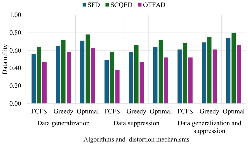
Experiments were conducted on a system equipped with an Intel^® Xeon^® Silver 4110 processor (2.10 GHz), 16 GB of memory, and a 1 TB HDD, running Microsoft Windows 10 (64-bit) Professional Edition. The implementation was developed and executed using Microsoft Visual Studio 2017 Community Edition and SQL Server 2017 RTM. Furthermore, the experimental evaluation was performed on three real-world opinion datasets, namely the Student Feedback Dataset (SFD) [60], the Student Course Quality Evaluation Dataset (SCQED) [61], and the Online Teaching Feedback Analytics Dataset (OTFAD) [62].

The Student Feedback Dataset (SFD) [60] is an opinion-oriented educational dataset composed of qualitative and quantitative feedback collected from students of a prominent university in North India. It is organized around six distinct institutional dimensions—teaching, course content, examination, lab work, library facilities, and extracurricular activities—each reflecting a critical aspect of academic and campus life. This dataset has 185 tuples. For every category, the student responses are recorded as free-text feedback accompanied by a ternary sentiment label encoded as −1 (negative), 0 (neutral), and 1 (positive), enabling both textual analysis and sentiment aggregation. The dataset exhibits a multi-category, low-cardinality structure with repeated sentiment values across categories, making it suitable for institutional-level analytics while also posing potential privacy risks due to small or homogeneous feedback groups. Its combination of subjective textual opinions, categorical context, and ordinal sentiment labels characterizes it as a semi-structured, sentiment-annotated dataset designed to support comprehensive institutional assessment and quality evaluation across multiple academic and non-academic services. To conduct the experiments effectively and maintain a controlled anonymization setting, only Feedback Category and Sentiment Polarity are designated as quasi-identifier attributes. The Examination attribute, which captures students’ opinions regarding examinations, is treated as the sensitive attribute. Although this setup restricts the sensitive attribute to a single opinion dimension, it remains sufficient to reveal clear and consistent trends in both effectiveness (data utility preservation) and efficiency (computational performance) of the proposed privacy-preserving mechanisms.

The Student Course Quality Evaluation Dataset (SCQED) [61] is a structured educational feedback dataset comprising approximately 1900 tuples, each representing a student’s evaluation of course quality across multiple instructional and experiential dimensions. Each entry corresponds to an individual learner’s perception of a specific course and captures both quantitative ratings and qualitative feedback, enabling comprehensive analysis of teaching effectiveness and learning outcomes. The dataset includes the detailed attributes that are related to instructional delivery (e.g., instructor clarity, teaching engagement, and responsiveness), course design (e.g., content quality, material usefulness, course pacing, and assignment quality), and learning experience (e.g., practical application, learning improvement, peer interaction, and class participation). In addition, contextual variables such as instruction mode (online, offline, or hybrid), study hours per week, attendance rate, prior knowledge level, and platform usability provide insight into environmental and learner-specific factors influencing course perception. Each record also contains a free-text feedback field, allowing for qualitative sentiment or thematic analysis, alongside a categorical Course_Quality_Label (Excellent, Good, Average, and Poor) that summarizes the student’s overall evaluation. This combination of fine-grained numerical ratings, behavioral indicators, and subjective textual feedback characterizes the dataset as a high-dimensional, mixed-type educational evaluation dataset, well suited for course quality assessment, learning analytics, and student satisfaction studies. For this dataset, to conduct the experiments effectively and maintain a controlled anonymization environment, the attributes Department, Course_ID, and Faculty_Experience are selected as the quasi-identifier attributes. The Student_Feedback attribute, which contains unstructured student opinions, is treated as the sensitive attribute. Although this configuration limits sensitivity to a single opinion-based dimension, it is sufficient to reveal clear and consistent trends in both effectiveness, measured in terms of data utility preservation, and efficiency, reflected in the computational performance of the proposed privacy-preserving mechanisms.

The Online Teaching Feedback Analytics Dataset (OTFAD) [62] is a mixed-type educational dataset comprising approximately 1400 student records collected from university-level online courses. It is designed to capture both subjective learner perceptions and objective academic indicators, enabling comprehensive analysis of online teaching effectiveness. Each record includes a free-text evaluation_text field that reflects students’ qualitative feedback and is suitable for sentiment or opinion mining, alongside a categorical sentiment_label (Positive, Neutral, or Negative) that summarizes the expressed attitude. In addition to textual feedback, the dataset incorporates multiple quantitative performance and engagement measures, such as satisfaction_score and engagement_score (rated on a 1–10 scale), platform_access_count reflecting system usage behavior, and academic outcomes including assignment_score and final_grade. The coexistence of behavioral, perceptual, and performance-based attributes characterizes the dataset as a multidimensional learning analytics resource, well suited for studying relationships between student engagement, satisfaction, online participation patterns, and learning outcomes in digital education environments. For this dataset, to conduct the experiments effectively and maintain a controlled anonymization environment, only the course_id, instructor_id, and timestamp attributes are designated as quasi-identifier attributes. The evaluation_text attribute, which contains unstructured student opinions, is treated as the sensitive attribute. Although this configuration restricts sensitivity to a single opinion-based dimension, it is sufficient to reveal clear and consistent trends in both effectiveness, measured in terms of data utility preservation, and efficiency, reflected in the computational performance of the proposed privacy-preserving mechanisms.

In addition, all experiments conducted in this study are based on the random selection of 185 tuples from each experimental dataset.

3.2. Experimental Results

3.2.1. Effect of d

In this section, we evaluate the impact of the parameter d on data utility under three anonymization strategies: data generalization, data suppression, and a hybrid approach combining generalization and suppression. All experimental settings are compared with k-Anonymity. For the experiments, with the proposed model, the parameters c and l are not considered (i.e., they do not influence the experimental results). The value of d in the proposed model and the value of k in k-Anonymity are varied from 2 to 8 to examine their effects on data utility.

From the experimental results presented in Figure 6a, it is evident that the proposed model exhibits behavior comparable to that of k-Anonymity when the parameters c and l are not taken into consideration. Under this condition, the proposed model effectively reduces to k-Anonymity. However, when all privacy parameters are incorporated, the proposed model provides enhanced privacy guarantees, thereby offering stronger preservation against potential disclosure risks. In addition, the proposed model demonstrates applicability in addressing privacy violation issues in content-based datasets. The results in Figure 6a further illustrate the impact of the parameter d under the data generalization strategy. In this strategy, unique quasi-identifier values are systematically replaced with more generalized representations, ensuring that each equivalence class contains at least d tuples. As d increases, deeper levels of generalization are required, resulting in a gradual and predictable increase in information loss while preserving all data tuples. The observed results reveal a smooth degradation in data utility and consistent trends across all evaluated datasets, indicating that generalization remains well suited for analytical applications. Nevertheless, for larger values of d, excessive generalization leads to diminished semantic granularity, thereby limiting the effectiveness of fine-grained data analysis. In contrast, the results shown in Figure 6b highlight the effects of the data suppression strategy. In this strategy, equivalence classes that fail to satisfy the specified threshold of d are removed entirely, thereby preserving the original precision of the remaining data. However, this strategy leads to a rapid reduction in the number of retained tuples. Consequently, data utility declines sharply and non-linearly as d increases, particularly in datasets characterized by sparse quasi-identifier distributions. This behavior renders suppression-only approaches impractical for larger values of d, due to substantial data loss and decreased representativeness.

The hybrid strategy, combining data generalization and suppression, is illustrated in Figure 6c. This method first applies generalization to mitigate the majority of privacy violations by aggregating quasi-identifier values into larger equivalence classes. Subsequently, selective suppression is employed to address any residual violations that cannot be resolved through acceptable levels of generalization. This two-stage process enhances overall effectiveness by minimizing unnecessary information loss while delaying tuple removal. As a result, the hybrid strategy achieves superior data utility across a broader range of d values. Empirical findings indicate that it consistently retains more usable data than suppression-only methods, while preserving greater semantic detail than pure generalization at higher levels of d. Therefore, the hybrid approach provides a well-balanced trade-off between privacy preservation and data utility, and demonstrates robust performance across all evaluated datasets.

3.2.2. Effect of c

This section is devoted to evaluating the impact of c on data utility. For the experiments, the value of d is fixed as 5, and the value of l is fixed as 0. The value of c is varied from 1.36 to 1.97 to examine how changes in the confidence constraint affect data utility. From the experimental results that are shown in Figure 7b, the experimental results consistently show a smooth and monotonic privacy–utility trade-off across all experimental datasets. Smaller values of c impose stricter upper bounds on the re-identification confidence of sensitive terms within each equivalence class, leading to more aggressive suppression of unique terms, consequently, lower retained data utility. Conversely, larger values of c relax the confidence constraint, allowing more sensitive terms to be preserved and substantially improving utility. Importantly, unlike tuple level suppression, confidence-based term suppression degrades utility in a gradual and controlled manner, preserving the structural integrity of the datasets. The experimental results also reveal that dataset characteristics play a crucial role, that the datasets with richer vocabularies and more diverse sensitive content (such as SCQED) are more resilient to strict confidence constraints, whereas datasets with repetitive or platform-specific terminology (such as OTFAD) experience lower utility degradation for low c. Overall, the results confirm that c is a powerful parameter for fine-grained regulation of attribute inference risk, with moderate values offering the best balance between strong privacy protection and meaningful analytical usability.

3.2.3. Effect of l

This section evaluates the impact of the parameter l on data utility. For the experiments, the value of d is fixed at 5, while the parameter c is not considered. All experiments in this section are compared with the l-diversity model. The value of l is varied from 2 to 8 in order to examine how changes in the diversity constraint affect data utility.

From the experimental results that are shown in Figure 7a, we can observe that, across all experimental datasets, the data utility achieved by l-Diversity is consistently higher than that of the proposed model. This observation can be attributed to the sensitive attribute, which primarily consists of comments and opinions characterized by highly diverse and nearly unique values. Consequently, each equivalence class formed under l-Diversity typically contains approximately l tuples. Despite this advantage in data utility, the proposed model provides stronger privacy preservation guarantees than l-Diversity. In particular, it is more effective in mitigating privacy violations in content-based datasets, where l-Diversity alone is often insufficient to prevent inference risks. Furthermore, the parameter l serves as a critical mechanism for controlling re-identification risks arising from rare or infrequently occurring sensitive terms within each equivalence class. Since the method suppresses sensitive terms that appear in at most l tuples, increasing l leads to more aggressive removal of rare and potentially identifying terms, resulting in a noticeable reduction in the utility of the semantic data. Nevertheless, this reduction in utility remains gradual and well controlled, as suppression is applied at the term level rather than the tuple level. This design preserves both the structural integrity of the dataset and the availability of tuples. As l increases, fewer terms are classified as uniquely identifying, allowing a greater proportion of sensitive content to be retained and thereby improving overall data utility. The results also demonstrate that dataset characteristics significantly influence robustness to l. Datasets with richer and more diverse vocabularies exhibit greater resilience to stricter l values, whereas datasets containing shorter or more repetitive content experience more rapid semantic degradation. Overall, these findings confirm that l provides an effective mechanism for controlling inference risks associated with rare terms, and that moderate values of l achieve a practical balance between strong privacy protection and meaningful analytical utility.

3.2.4. Effect of the Combined Privacy Preservation Parameters on Data Utility

In this section, the experimental evaluation of the combined privacy parameters as d, c, and l (i.e., d, d and c, d and l, and all privacy preservation such that d, c, and l) highlights that privacy protection in practice is governed by interactions between structural anonymity and term-level inference controls, rather than isolated parameter effects. For the experiments, the value of d, c, and l is fixed as 5. From the experimental results that are shown in Figure 7c, the enlargement of equivalence classes imposed by d substantially reduces the dominance of individual sensitive terms, thereby lowering the re-identification confidence that c is designed to constrain. As a result, the confidence-based suppression triggered by c becomes less frequent and more targeted, leading to smoother utility degradation than when c is applied alone. This interaction makes d and c especially effective against dominance-based inference attacks while retaining much of the semantic integrity of the sensitive attributes. With d and l, the structural grouping enforced by d increases the frequency of sensitive terms within each equivalence class, effectively transforming many rare or near-unique terms into common ones. Consequently, fewer sensitive terms violate the occurrence threshold specified by l, and term-level suppression is delayed or reduced. This explains why d and l consistently preserve more semantic content than applying l in isolation, particularly in datasets with sparse quasi-identifiers. The experiments show that d and l are especially effective for mitigating uniqueness-based inference risks without causing abrupt utility loss, as suppression is applied only to truly rare identifiers that remain after equivalence-class formation. The full privacy preservation consideration parameters (i.e., all privacy preservation parameters as d, c, and l are considered) show the strongest and most stable performance across all datasets because it simultaneously addresses both extremes of inference risk. That is, overly frequent (dominant) terms controlled by c and infrequent (unique) terms controlled by l, with d providing the structural foundation that stabilizes both mechanisms. In this configuration, generalization through d absorbs most privacy pressure, c suppresses residual high-confidence terms, and l removes remaining rare identifiers. This layered enforcement leads to selective, minimal suppression and avoids the over-generalization seen in single-parameter approaches. Empirically, d, c, and l consistently yield the highest remaining data utility and the most gradual degradation curves, demonstrating superior robustness to dataset sparsity and variability. Overall, the results confirm that the combined use of d, c, and l produces a synergistic effect, delivering stronger privacy guarantees with better preserved analytical usefulness than any pairwise combination or single parameter.

3.2.5. Effect of Dataset Sizes

In this section, we investigate the impact of data generalization and dataset size on data utility. In the experimental setup, the parameters d and l are fixed at 5 to isolate the effects of generalization and dataset scale, while the parameter c is set to 1.49. The dataset size is varied from 10% to 100% to systematically assess its influence on data utility.

From the experimental results that are shown in Figure 8a–c, the impact of dataset size is analyzed under three privacy mechanisms: data generalization, data suppression, and a hybrid approach that combines generalization and suppression, respectively. The results clearly demonstrate that data utility improves steadily and consistently as the dataset size increases, confirming that larger datasets are inherently better able to satisfy strict privacy constraints while preserving analytical value. At smaller dataset sizes (approximately 10–30%), data utility remains relatively low across all datasets. This behavior can be attributed to two primary factors. First, the limited data volume restricts the formation of equivalence classes, necessitating aggressive quasi-identifier generalization and suppression to satisfy the requirement that each equivalence class contains at least five tuples. Second, with fewer tuples per class, sensitive terms tend to exhibit higher dominance or rarity, increasing the likelihood of violating the confidence constraint c and the rarity constraint l, thereby triggering more frequent term suppression. Consequently, both structural abstraction and semantic information loss are amplified in data-scarce scenarios. As the dataset size increases to a moderate range (40–70%), the effects of the privacy constraints become more balanced. Larger datasets enable more natural formation of equivalence classes, reducing the extent of generalization and suppression required to satisfy the d constraint. In addition, sensitive terms appear more frequently within equivalence classes, lowering their re-identification risk and reducing suppression imposed by the c and l constraints. This phase represents a stabilization region, in which increasing data volume leads to substantial improvements in utility while maintaining a consistent level of privacy protection. For larger dataset sizes (80–100%), data utility approaches its maximum, with only marginal improvements observed beyond this range. In this regime, equivalence classes are well populated, generalization remains shallow, and most sensitive terms satisfy both confidence-based and occurrence-based constraints. As a result, term-level suppression becomes infrequent, and the retained data preserves a high degree of semantic richness. These findings indicate that generalization-based $(d,c,l)$-privacy scales effectively with increasing dataset size, provided that sufficient data is available. Differences among datasets further highlight the influence of data characteristics. The SCQED dataset consistently achieves the highest utility due to its structured and dense quasi-identifier distribution, which supports stable equivalence class formation, as well as its rich vocabulary, which mitigates dominance and rarity risks. The SFD dataset exhibits moderate sensitivity, reflecting its relatively constrained quasi-identifier domain. In contrast, the OTFAD dataset remains the most sensitive due to its sparse and high-dimensional quasi-identifier combinations. Nevertheless, all datasets, including OTFAD, benefit significantly from increased data volume, underscoring the universal importance of dataset size in privacy preservation data analysis. Overall, these results confirm that dataset size is a critical factor in determining data utility under fixed $(d,c,l)$-Privacy constraints. Adequate data volume not only stabilizes equivalence class formation but also reduces confidence-based and rarity-based inference risks at the term level. Therefore, in practical applications of generalization-based privacy mechanisms, ensuring sufficient dataset size is essential for achieving strong privacy protection while maintaining meaningful analytical utility.

3.2.6. Effect of the Proposed Privacy Preservation Algorithms

In this section, we evaluate the impact of the proposed privacy preservation algorithms (i.e., FCFS, greedy, and optimal algorithms) on data utility. In the experimental setup, the parameters d and l are fixed at 5 to isolate their effects, while the parameter c is set to 1.49 to maintain a consistent level of confidence constraint across all experiments.

From the experimental results shown in Figure 9, a clear and consistent hierarchy emerges among the evaluated algorithms. When only data generalization is applied, the optimal algorithm consistently achieves the highest data utility across all experimental datasets, followed by the greedy algorithm, while the FCFS algorithm yields the lowest utility. This pattern reflects the effectiveness of optimization-aware equivalence class construction in minimizing unnecessary generalization, particularly for datasets with well-structured quasi-identifiers such as SCQED. When data suppression alone is applied, data utility declines noticeably for all algorithms, indicating that suppression introduces greater information loss than generalization. This effect is especially pronounced for the OTFAD dataset, where temporal and textual attributes are highly sensitive to record removal. Despite this overall reduction, the relative ranking of the algorithms remains unchanged, demonstrating that the equivalence class construction strategy is the dominant factor influencing data utility. In the hybrid scenario, where data generalization is combined with data suppression, data utility improves compared with the suppression-only approach but remains lower than that achieved through generalization alone. This suggests that generalization mitigates part of the information loss introduced by suppression while still satisfying privacy constraints. Across all scenarios, the optimal algorithm consistently preserves the highest level of data utility, while the greedy algorithm offers a strong and stable intermediate performance. In contrast, the FCFS algorithm exhibits the greatest level of data distortion due to its rigid, order-based equivalence class construction. Overall, these findings highlight that the strategy used to construct equivalence classes has a more substantial impact on data utility than the choice of distortion mechanism. Consequently, globally or locally optimized approaches are essential for maintaining high data utility while satisfying privacy requirements.

4. Conclusions

This paper investigates $(d,c,l)$-Privacy as an effective privacy preservation model for releasing datasets containing sensitive information, particularly in content-based and text-rich domains. By jointly enforcing constraints on equivalence class size d, re-identification confidence c, and sensitive value diversity l, the $(d,c,l)$-Privacy model provides stronger protection against both identity disclosure and attribute inference compared with traditional privacy models. To evaluate its practical applicability, three equivalence-class construction algorithms—First Come First Serve (FCFS), Greedy, and Optimal—are developed using a combination of data generalization and data suppression. Experimental results demonstrate that all three algorithms successfully satisfy the $(d,c,l)$-Privacy constraints, thereby preventing privacy breaches in released datasets. However, the findings clearly indicate that the choice of equivalence-class construction strategy has a significant impact on data utility. The FCFS algorithm achieves the highest computational efficiency due to its order-based and low-complexity design, making it suitable for scenarios requiring rapid anonymization. However, its strict reliance on tuple order often leads to substantial information loss. The Greedy algorithm offers a more balanced approach, preserving data semantics while maintaining acceptable computational costs, and consistently achieves higher data utility than FCFS. In contrast, the Optimal algorithm maximizes data utility by globally minimizing information loss, thereby establishing an upper bound on achievable utility, albeit at the expense of increased computational complexity. Overall, the experimental results confirm that $(d,c,l)$-Privacy is a robust and practical framework for privacy-preserving data publishing, capable of effectively balancing privacy protection and data utility in real-world data-sharing scenarios. While the FCFS algorithm is well suited for time-critical applications, the Greedy and Optimal algorithms are more appropriate for contexts where preserving data utility is paramount. These findings underscore the importance of optimization-aware equivalence-class construction and demonstrate that $(d,c,l)$-Privacy can be effectively applied across diverse datasets to support secure and meaningful data release.

5. Future Work

Although the proposed model effectively addresses privacy violations in content-based datasets, adversaries may develop increasingly sophisticated techniques capable of compromising privacy. Therefore, there is a need for more advanced privacy preservation models that can proactively identify and mitigate emerging privacy threats in content-based data environments.

A promising direction is to combine the proposed model with AI-based privacy preservation mechanisms. The proposed model can be applied first to produce a sanitized dataset for release, while techniques such as differentially private fine-tuning, federated learning, or homomorphic encryption can be applied afterward to protect any models trained on top of it. Another important direction is to strengthen the model against inference attacks driven by large language models, which can recover personal attributes from anonymized text by exploiting subtle contextual cues that traditional de-identification tools overlook. Finally, the proposed model can be extended to multilingual and streaming content-based datasets, where vocabulary, semantic structure, and the rate of incoming records differ substantially from the datasets considered in this study.

References

1. Sweeney, L. k-anonymity: A model for protecting privacy. Int. J. Uncertain. Fuzziness Knowl. Based Syst. 2002, 10, 557–570. [Google Scholar] [CrossRef]
2. Slijepčević, D.; Henzl, M.; Klausner, L.D.; Dam, T.; Kieseberg, P.; Zeppelzauer, M. k-anonymity in practice: How generalisation and suppression affect machine learning classifiers. Comput. Secur. 2021, 111, 102488. [Google Scholar] [CrossRef]
3. Li, S.; Schneider, M.J.; Yu, Y.; Gupta, S. Reidentification risk in panel data: Protecting for k-anonymity. Inf. Syst. Res. 2023, 34, 1066–1088. [Google Scholar] [CrossRef]
4. De Pascale, D.; Cascavilla, G.; Tamburri, D.A.; Van Den Heuvel, W.J. Real-world K-Anonymity applications: The KGen approach and its evaluation in fraudulent transactions. Inf. Syst. 2023, 115, 102193. [Google Scholar] [CrossRef]
5. Ren, W.; Ghazinour, K.; Lian, X. kt-Safety: Graph Release via k-Anonymity and t-Closeness. IEEE Trans. Knowl. Data Eng. 2022, 35, 9102–9113. [Google Scholar] [CrossRef]
6. Majeed, A.; Hwang, S.O. Differential privacy and k-anonymity-based privacy preserving data publishing scheme with minimal loss of statistical information. IEEE Trans. Comput. Soc. Syst. 2023, 11, 3753–3765. [Google Scholar] [CrossRef]
7. Sangaiah, A.K.; Javadpour, A.; Ja’fari, F.; Pinto, P.; Chuang, H.M. Privacy-aware and ai techniques for healthcare based on k-anonymity model in internet of things. IEEE Trans. Eng. Manag. 2023, 71, 12448–12462. [Google Scholar] [CrossRef]
8. Nadkarni, P.M.; Ohno-Machado, L.; Chapman, W.W. Natural language processing: An introduction. J. Am. Med. Inform. Assoc. 2011, 18, 544–551. [Google Scholar] [CrossRef]
9. Kang, Y.; Cai, Z.; Tan, C.W.; Huang, Q.; Liu, H. Natural language processing (NLP) in management research: A literature review. J. Manag. Anal. 2020, 7, 139–172. [Google Scholar] [CrossRef]
10. Chowdhary, K. Natural language processing. In Fundamentals of Artificial Intelligence; Springer: Berlin/Heidelberg, Germany, 2020; pp. 603–649. [Google Scholar]
11. Khurana, D.; Koli, A.; Khatter, K.; Singh, S. Natural language processing: State of the art, current trends and challenges. Multimed. Tools Appl. 2023, 82, 3713–3744. [Google Scholar] [CrossRef]
12. Chen, Z.; Cheng, X.; Dong, S.; Dou, Z.; Guo, J.; Huang, X.; Lan, Y.; Li, C.; Li, R.; Liu, T.Y.; et al. Information retrieval: A view from the Chinese IR community. Front. Comput. Sci. 2021, 15, 151601. [Google Scholar] [CrossRef]
13. Wang, J.; Huang, J.X.; Tu, X.; Wang, J.; Huang, A.J.; Laskar, M.T.R.; Bhuiyan, A. Utilizing bert for information retrieval: Survey, applications, resources, and challenges. ACM Comput. Surv. 2024, 56, 1–33. [Google Scholar] [CrossRef]
14. Sivarajkumar, S.; Mohammad, H.A.; Oniani, D.; Roberts, K.; Hersh, W.; Liu, H.; He, D.; Visweswaran, S.; Wang, Y. Clinical information retrieval: A literature review. J. Healthc. Inform. Res. 2024, 8, 313–352. [Google Scholar] [CrossRef]
15. Bouadjenek, M.R.; Hacid, H.; Bouzeghoub, M. Social networks and information retrieval, how are they converging? A survey, a taxonomy and an analysis of social information retrieval approaches and platforms. Inf. Syst. 2016, 56, 1–18. [Google Scholar] [CrossRef]
16. Blum, A.; Dwork, C.; McSherry, F.; Nissim, K. Practical privacy: The SuLQ framework. In Proceedings of the Twenty-Fourth ACM SIGMOD-SIGACT-SIGART Symposium on Principles of Database Systems, Baltimore, MD, USA, 13–15 June 2005; Association for Computing Machinery: New York, NY, USA, 2005; pp. 128–138. [Google Scholar]
17. Li, J.; Liu, Z.; Chen, X.; Xhafa, F.; Tan, X.; Wong, D.S. L-EncDB: A lightweight framework for privacy-preserving data queries in cloud computing. Knowl. Based Syst. 2015, 79, 18–26. [Google Scholar] [CrossRef]
18. Memon, I.; Arain, Q.A. Dynamic path privacy protection framework for continuous query service over road networks. World Wide Web 2017, 20, 639–672. [Google Scholar] [CrossRef]
19. Ji, S.; Mittal, P.; Beyah, R. Graph data anonymization, de-anonymization attacks, and de-anonymizability quantification: A survey. IEEE Commun. Surv. Tutor. 2016, 19, 1305–1326. [Google Scholar] [CrossRef]
20. Murthy, S.; Bakar, A.A.; Rahim, F.A.; Ramli, R. A comparative study of data anonymization techniques. In 2019 IEEE 5th Intl Conference on Big Data Security on Cloud (BigDataSecurity), IEEE Intl Conference on High Performance and Smart Computing, (HPSC) and IEEE Intl Conference on Intelligent Data and Security (IDS); IEEE: Piscataway, NJ, USA, 2019; pp. 306–309. [Google Scholar]
21. Olatunji, I.E.; Rauch, J.; Katzensteiner, M.; Khosla, M. A review of anonymization for healthcare data. Big Data 2024, 12, 538–555. [Google Scholar] [CrossRef] [PubMed]
22. Shamsinejad, E.; Banirostam, T.; Pedram, M.M.; Rahmani, A.M. A review of anonymization algorithms and methods in big data. Ann. Data Sci. 2025, 12, 253–279. [Google Scholar] [CrossRef]
23. Bafna, P.; Pramod, D.; Vaidya, A. Document clustering: TF-IDF approach. In 2016 International Conference on Electrical, Electronics, and Optimization Techniques (ICEEOT); IEEE: Piscataway, NJ, USA, 2016; pp. 61–66. [Google Scholar]
24. Khan, R.; Qian, Y.; Naeem, S. Extractive based text summarization using k-means and tf-idf. Int. J. Inf. Eng. Electron. Bus. 2019, 13, 33. [Google Scholar]
25. Surianto, D.F.; Surianto, D.F. Enhancing K-Means Clustering for Journal Articles using TF-IDF and LDA Feature Extraction. Brill. Res. Artif. Intell. 2024, 4, 964–972. [Google Scholar] [CrossRef]
26. Kim, S.W.; Gil, J.M. Research paper classification systems based on TF-IDF and LDA schemes. Hum. Centric Comput. Inf. Sci. 2019, 9, 30. [Google Scholar] [CrossRef]
27. Zhou, Z.; Qin, J.; Xiang, X.; Tan, Y.; Liu, Q.; Xiong, N.N. News Text Topic Clustering Optimized Method Based on TF-IDF Algorithm on Spark. Comput. Mater. Contin. 2020, 62, 217. [Google Scholar] [CrossRef]
28. Acar, A.; Aksu, H.; Uluagac, A.S.; Conti, M. A survey on homomorphic encryption schemes: Theory and implementation. ACM Comput. Surv. (Csur) 2018, 51, 1–35. [Google Scholar] [CrossRef]
29. Yi, X.; Paulet, R.; Bertino, E. Homomorphic encryption. In Homomorphic Encryption and Applications; Springer: Berlin/Heidelberg, Germany, 2014; pp. 27–46. [Google Scholar]
30. Ogburn, M.; Turner, C.; Dahal, P. Homomorphic encryption. Procedia Comput. Sci. 2013, 20, 502–509. [Google Scholar] [CrossRef]
31. Naehrig, M.; Lauter, K.; Vaikuntanathan, V. Can homomorphic encryption be practical? In Proceedings of the 3rd ACM Workshop on Cloud Computing Security Workshop, Chicago, IL, USA, 21 October 2011; Association for Computing Machinery: New York, NY, USA, 2011; pp. 113–124. [Google Scholar]
32. Dwork, C. Differential privacy. In Proceedings of the International Colloquium on Automata, Languages, and Programming; Springer: Berlin/Heidelberg, Germany, 2006; pp. 1–12. [Google Scholar]
33. El Ouadrhiri, A.; Abdelhadi, A. Differential privacy for deep and federated learning: A survey. IEEE Access 2022, 10, 22359–22380. [Google Scholar] [CrossRef]
34. Dong, J.; Roth, A.; Su, W.J. Gaussian differential privacy. J. R. Stat. Soc. Ser. B Stat. Methodol. 2022, 84, 3–37. [Google Scholar] [CrossRef]
35. Ponomareva, N.; Hazimeh, H.; Kurakin, A.; Xu, Z.; Denison, C.; McMahan, H.B.; Vassilvitskii, S.; Chien, S.; Thakurta, A.G. How to DP-fy ML: A Practical Guide to Machine Learning with Differential Privacy. J. Artif. Intell. Res. 2023, 77, 1113–1201. [Google Scholar] [CrossRef]
36. Guan, H.; Yap, P.T.; Bozoki, A.; Liu, M. Federated learning for medical image analysis: A survey. Pattern Recognit. 2024, 151, 110424. [Google Scholar] [CrossRef]
37. Ye, M.; Fang, X.; Du, B.; Yuen, P.C.; Tao, D. Heterogeneous federated learning: State-of-the-art and research challenges. ACM Comput. Surv. 2023, 56, 1–44. [Google Scholar] [CrossRef]
38. Li, H.; Li, C.; Wang, J.; Yang, A.; Ma, Z.; Zhang, Z.; Hua, D. Review on security of federated learning and its application in healthcare. Future Gener. Comput. Syst. 2023, 144, 271–290. [Google Scholar] [CrossRef]
39. Xiao, X.; Tao, Y. Anatomy: Simple and Effective Privacy Preservation. In Proceedings of the 32nd International Conference on Very Large Data Bases (VLDB ’06); VLDB Endowment: Boston, MA, USA, 2006; pp. 139–150. [Google Scholar]
40. Susan, V.S.; Christopher, T. Anatomisation with Slicing: A New Privacy Preservation Approach for Multiple Sensitive Attributes. SpringerPlus 2016, 5, 964. [Google Scholar] [CrossRef]
41. Cao, J.; Karras, P.; Kalnis, P.; Tan, K.L. SABRE: A Sensitive Attribute Bucketization and REdistribution Framework for t-Closeness. VLDB J. 2011, 20, 59–81. [Google Scholar] [CrossRef]
42. Hong, T.P.; Lin, C.W.; Yang, K.T.; Wang, S.L. Using TF-IDF to hide sensitive itemsets. Appl. Intell. 2013, 38, 502–510. [Google Scholar] [CrossRef]
43. Kasar, N.; Phad, V.S. TF-IDF and KDC based Privacy Preserving Multi keyword Search over Distributed Encrypted Documents. Int. J. Adv. Res. Comput. Commun. Eng. (IJARCCE) 2016, 5, 645–648. [Google Scholar]
44. Ma, X.; Chang, X.; Chen, H. Differential privacy protection algorithm for network sensitive information based on singular value decomposition. Sci. Rep. 2023, 13, 6035. [Google Scholar] [CrossRef]
45. Babu, T.G.; Anitha, E. Privacy Preserving Collaborative Model Document Clustering Using TF-IDF Approach. Int. J. Sci. Res. Sci. Eng. Technol. (IJSRSET) 2018, 4, 615–627. [Google Scholar]
46. Hassan, F.; Sánchez, D.; Soria-Comas, J.; Domingo-Ferrer, J. Automatic Anonymization of Textual Documents: Detecting Sensitive Information via Word Embeddings. In 2019 18th IEEE International Conference on Trust, Security and Privacy in Computing and Communications/13th IEEE International Conference on Big Data Security on Cloud (TrustCom/BigDataSecurity); IEEE: Piscataway, NJ, USA, 2019; pp. 358–365. [Google Scholar]
47. Abadi, M.; Chu, A.; Goodfellow, I.; McMahan, H.B.; Mironov, I.; Talwar, K.; Zhang, L. Deep Learning with Differential Privacy. In Proceedings of the 2016 ACM SIGSAC Conference on Computer and Communications Security (CCS ’16), New York, NY, USA, 24–28 October 2016; pp. 308–318. [Google Scholar] [CrossRef]
48. Yu, D.; Naik, S.; Backurs, A.; Gopi, S.; Inan, H.A.; Kamath, G.; Kulkarni, J.; Lee, Y.T.; Manoel, A.; Wutschitz, L.; et al. Differentially Private Fine-Tuning of Language Models. In Proceedings of the International Conference on Learning Representations (ICLR), Online, 25–29 April 2022. [Google Scholar]
49. Lison, P.; Pilán, I.; Sánchez, D.; Batet, M.; Øvrelid, L. Anonymisation Models for Text Data: State of the Art, Challenges and Future Directions. In Proceedings of the 59th Annual Meeting of the Association for Computational Linguistics and the 11th International Joint Conference on Natural Language Processing (ACL-IJCNLP); Association for Computational Linguistics: Stroudsburg, PA, USA, 2021; pp. 4188–4203. [Google Scholar] [CrossRef]
50. Pilán, I.; Lison, P.; Øvrelid, L.; Papadopoulou, A.; Sánchez, D.; Batet, M. The Text Anonymization Benchmark (TAB): A Dedicated Corpus and Evaluation Framework for Text Anonymization. Comput. Linguist. 2022, 48, 1053–1101. [Google Scholar] [CrossRef]
51. Liu, Y.; Yao, Y.; Ton, J.F.; Zhang, X.; Guo, R.; Cheng, H.; Klochkov, Y.; Taufiq, M.F.; Li, H. Trustworthy LLMs: A Survey and Guideline for Evaluating Large Language Models’ Alignment. In Proceedings of the International Conference on Learning Representations (ICLR), Vienna, Austria, 7–11 May 2024. [Google Scholar]
52. Kotelnikov, A.; Baranchuk, D.; Rubachev, I.; Babenko, A. TabDDPM: Modelling Tabular Data with Diffusion Models. In Proceedings of the 40th International Conference on Machine Learning (ICML), Honolulu, HI, USA, 23–29 July 2023; Proceedings of Machine Learning Research (PMLR): Honolulu, HI, USA, 2023; Volume 202, pp. 17564–17579. [Google Scholar]
53. Borisov, V.; Seßler, K.; Leemann, T.; Pawelczyk, M.; Kasneci, G. Language Models are Realistic Tabular Data Generators. In Proceedings of the International Conference on Learning Representations (ICLR), Kigali, Rwanda, 1–5 May 2023. [Google Scholar]
54. Hu, Y.; Wu, F.; Li, Q.; Long, Y.; Garrido, G.M.; Ge, C.; Ding, B.; Forsyth, D.; Li, B.; Song, D. SoK: Privacy-Preserving Data Synthesis. In 2024 IEEE Symposium on Security and Privacy (SP); IEEE: Piscataway, NJ, USA, 2024; pp. 4696–4713. [Google Scholar] [CrossRef]
55. Li, T.; Sahu, A.K.; Talwalkar, A.; Smith, V. Federated Learning: Challenges, Methods, and Future Directions. IEEE Signal Process. Mag. 2020, 37, 50–60. [Google Scholar] [CrossRef]
56. Wang, B.; Li, H.; Guo, Y.; Wang, J. PPFLHE: A Privacy-Preserving Federated Learning Scheme with Homomorphic Encryption for Healthcare Data. Appl. Soft Comput. 2023, 146, 110677. [Google Scholar] [CrossRef]
57. Paschos, V.T. An overview on polynomial approximation of NP-hard problems. Yugosl. J. Oper. Res. 2009, 19, 3–40. [Google Scholar] [CrossRef]
58. Garey, M.R.; Johnson, D.S. Computers and Intractability: A Guide to the Theory of NP-Completeness; W. H. Freeman & Co.: New York, NY, USA, 1979. [Google Scholar]
59. Machanavajjhala, A.; Kifer, D.; Gehrke, J.; Venkitasubramaniam, M. L-diversity: Privacy beyond k-anonymity. ACM Trans. Knowl. Discov. Data (TKDD) 2007, 1, 3-es. [Google Scholar] [CrossRef]
60. Brar, A.R. Student Feedback Dataset. 2018. Available online: https://www.kaggle.com/datasets/brarajit18/student-feedback-dataset (accessed on 18 April 2026).
61. Python Developer. Student Course Quality Evaluation Dataset. 2023. Available online: https://www.kaggle.com/datasets/programmer3/student-course-quality-evaluation-dataset (accessed on 18 April 2026).
62. Python Developer. Online Teaching Feedback Analytics Dataset. Available online: https://www.kaggle.com/datasets/programmer3/online-teaching-feedback-analytics-dataset (accessed on 18 April 2026).
Figure 1. Domain Generalization Hierarchies (DGHs) for the quasi-identifier attributes of Table 3: (a) Gender; (b) Datetime; (c) Education, where higher levels correspond to more generalized values.
Mathematics 14 01896 g001
Figure 2. A completed graph of 3-vertices.
Mathematics 14 01896 g002
Figure 3. An example graph of X 3 C problem.
Mathematics 14 01896 g003
Figure 4. The solution graph S 1 , representing one feasible solution to the X 3 C instance, where bold solid edges denote the selected exact-cover subsets and dashed edges denote the remaining non-solution edges.
Mathematics 14 01896 g004
Figure 5. The solution graph S 2 , representing one feasible solution to the X 3 C instance, where bold solid edges denote the selected exact-cover subsets and dashed edges denote the remaining non-solution edges.
Mathematics 14 01896 g005
Figure 6. Effect of d on retained data utility, comparing ( d , c , l ) -Privacy with k-Anonymity: (a) generalization; (b) suppression; (c) combined generalization and suppression.
Mathematics 14 01896 g006
Figure 7. Effect of c, l, and their combinations on retained data utility: (a) comparison with l-Diversity for varying l; (b) effect of c; (c) effect of combined privacy parameters.
Mathematics 14 01896 g007
Figure 8. Effect of dataset size on retained data utility under fixed ( d , c , l ) -Privacy parameters: (a) generalization; (b) suppression; (c) combined generalization and suppression.
Mathematics 14 01896 g008
Figure 9. Effect of the proposed FCFS, Greedy, and Optimal algorithms on retained data utility under data generalization, data suppression, and their combination.
Mathematics 14 01896 g009