Cost-Based Competition and Market Share Determination: A CES Analytical Framework

Abstract

This study examines the micro-level mechanisms through which increasing market concentration and the entrenchment of competitive advantage arise. We develop a theoretical framework based on a constant elasticity of substitution (CES) production function and a CES demand structure, integrating—within a unified analytical chain—firms’ inter-firm cost competition, cost-plus pricing, demand allocation, and market-share decision-making. Methodologically, we first derive the relationship between firm prices and productivity from cost minimization and optimal pricing rules and then obtain explicit expressions for market shares and sales under CES demand. We subsequently introduce endogenous learning effects, in which firms’ market shares feed into future productivity growth via a learning curve mechanism, thereby characterizing the conversion of static advantage into dynamic competitive advantage. We further incorporate technology-factor substitutions, such as robotics, into firms’ production and cost structures to analyze how cost savings and efficiency gains accelerate the evolution of concentration and to show how learning disadvantages induced by insufficient market shares deter potential entry. The results indicate that firms’ market shares are primarily determined by their relative productivity, while profits respond asymmetrically to productivity differentials. Learning and technological substitution support the accumulation of advantages for incumbent firms and endogenously generate barriers to entry. Overall, this paper explains how the entrenchment of competitive advantage is reinforced through dynamic feedback, driving industries toward higher levels of concentration.

1. Introduction

In the context of the global economy, the continuous rise in market concentration and the entrenchment of competitive advantage have become increasingly prominent, emerging as central issues in industrial organization theory and competition policy [1,2,3,4,5,6,7,8]. In particular, amid the current wave of a new industrial revolution characterized by digitalization and automation, the rapid development and adoption of disruptive innovations such as robotics not only fundamentally alter firms’ production processes and cost structures but may also accelerate this trend under existing market mechanisms—thereby strengthening the advantages of leading firms to an unprecedented degree and further shaping innovation, employment, and income distribution [9,10,11,12,13,14,15,16,17]. In parallel, recent research on artificial intelligence highlights that the scaling of intelligent technologies similarly drives market concentration and creates new forms of entry barriers [18]. Therefore, it is of both theoretical and practical significance to investigate how firms’ relative advantages are transformed from productivity differentials into long-run market power through market interaction mechanisms, how this transformation interacts with frontier technological innovation, and how it can endogenously drive industry concentration.

At the level of static analysis, firms’ heterogeneity is the starting point for understanding both market structure and divergence in performance. Productivity differences are widely regarded as a key driver of performance heterogeneity across firms [19,20]. Within a monopolistic competition framework, more efficient firms typically face lower marginal costs, which provides the basis for their advantage in price competition. Autor et al. (2020) [21] and Firooz et al. (2025) [22] demonstrate that automation technologies, including robotics, amplify the “superstar firm” effect, enabling high-productivity firms to capture disproportionately large market shares and profits. The classic model of Dixit and Stiglitz (1977) [23], along with subsequent developments, employs constant elasticity of substitution (CES) preferences, thereby offering a standard toolkit for analyzing firms’ pricing decisions, demand allocation, and market shares [24]. Firms often adopt cost-plus pricing strategies [25], in which the optimal price is closely related to marginal cost and the demand substitution elasticity. Against this backdrop, the introduction of automation technologies such as robots can, by significantly raising labor productivity and streamlining production processes, directly reduce firms’ marginal costs [26,27,28]. This productivity advantage can be translated into a pricing advantage, and—through the CES demand structure—allows firms equipped with advanced automation technology to obtain higher sales and larger market shares [29].

However, the evolution of market concentration is not merely a mechanical reflection of static efficiency differences. Empirical evidence suggests that disparities in market share not only persist but are often accompanied by systematic dynamic amplification effects. Cross-country evidence from Bajgar et al. (2025) [30] shows that industry concentration and markups have risen in both Europe and North America, indicating a pervasive trend. Dynamic theories underscore the pivotal roles played by learning effects and cumulative advantages in the evolution of market structure. Arrow (1962)’s “learning by doing” framework posits that firms can continuously reduce unit costs and improve efficiency through the accumulation of production experience [31]. This implies that a firm that secures an early market-share advantage not only operates at a larger scale, but also benefits from a faster pace of experience accumulation, thereby further accelerating productivity growth and establishing a positive feedback loop [32,33]. Aghion et al. (2023) [34] provide a theory of falling growth and rising rents, showing that when growth slows, incumbent firms can extract higher rents, further solidifying their dominant positions. In particular, the deployment of automation technologies such as robots is typically associated with substantial fixed investment and technological learning costs [9,35,36]. Once a firm successfully deploys and masters these technologies, its advantages in production efficiency and costs become increasingly difficult to imitate. Moreover, such advantages can be sustained and further widened through scale economies and learning-by-doing effects, thereby extending the gap relative to competitors [7]. Dynamic industrial organization theory also extensively examines the complex processes of firm entry, exit, growth, and decline. Within this framework, the sustained expansion of leading firms and the marginalization of laggards are viewed as the joint outcomes of cumulative advantages and failure to catch up [27,37].

Although both static and dynamic analyses offer important perspectives for understanding market concentration, existing research still faces challenges in building an integrated framework. Many models either examine the static effects of productivity on market share in isolation or treat learning effects as a relatively exogenous dynamic process, without rigorously capturing the closed-loop feedback among productivity, market share, profits, and learning within a unified setting. In addition, theories of entry barriers often emphasize structural factors such as fixed costs, sunk costs, or economies of scale [38], but have paid relatively less attention to how incumbents’ productivity can be continuously enhanced through ongoing learning and technological innovation (e.g., robot adoption). Specifically, these improvements may dynamically erode prospective entrants’ expected profits, thereby endogenously generating entry barriers. This “catch-up gap” constraint arising from the accumulation of dynamic advantages is crucial for understanding the path dependence of industry concentration—particularly in the context of accelerating technological change.

This paper aims to bridge the aforementioned research gap by theoretically deriving rigorous mathematical propositions. Through the construction of a unified theoretical framework, this study comprehensively analyzes the micro-mechanisms underlying the increase in market concentration and the entrenchment of competitive advantages. In particular, it highlights the accelerating role of technological innovations in automation, such as robotics, thereby laying a solid analytical foundation for future empirical validation. Specifically, this paper first establishes a static analytical chain—productivity → costs → pricing → CES demand → market share → profits—and rigorously derives how a firm’s market share is determined by its relative productivity. It also uncovers the asymmetric sensitivity of profits to productivity differences, namely that high-productivity firms can translate efficiency advantages into profit advantages more substantially [11]. We then focus on how robot technology operates as a vehicle for productivity improvement, thereby intensifying the accumulation of such advantages. Building on this static foundation, we further introduce endogenous learning effects, allowing a firm’s market share to shape its future productivity growth through a learning curve mechanism [31]. This extension transforms static advantages into dynamic ones. Taken together, this integrated mechanism explains how market leaders achieve continuous productivity gains through sustained learning and early investment in, as well as optimization of, cutting-edge technologies such as robots. Finally, we show that potential entrants, due to insufficient initial market share, are unable to catch up with incumbents effectively in the learning race. This difficulty is especially pronounced as barriers related to automation technologies become increasingly stringent, leading to an endogenous formation of entry barriers and, consequently, driving the industry toward higher levels of concentration.

Herein, the main contributions can be summarized in three aspects: Firstly, an integrated theoretical framework. We develop a complete and highly coherent theoretical system that embeds the dynamic feedback relationship among productivity (including the contribution of robotics), cost-plus pricing, CES demand, market share, profits, and learning effects within a unified setting. This provides a consistent microeconomic explanation for the entrenchment of competitive advantages. Secondly, asymmetric sensitivity of profits to productivity differences. This paper explicitly identifies a substantial and asymmetric sensitivity of profits to productivity gaps. We further show that the substitution elasticity magnifies the advantage of high-productivity firms and accelerates the concentration of profit distributions—an effect that is even stronger in the presence of technology-enhanced capabilities such as robotics. Thirdly, endogenizing entry-barrier formation via dynamic learning. By characterizing the shrinkage of the “catch-up space” induced by dynamic learning, we endogenize the mechanism underlying the formation of entry barriers. Specifically, incumbents’ ongoing learning and their early adoption, mastery, and optimization of robotic technologies reduce potential entrants’ expected returns, thereby deterring entry. This deepens our understanding of the path dependence of industry concentration.

2. Model

2.1. Model Setup

When analyzing firms’ competitiveness, we first need to build a theoretical framework that characterizes the relationships among production costs, product prices, sales, and market share. Arrow (1962) point out that the CES production function can flexibly reflect the substitutability among different inputs [31,39], and it also nests the Cobb–Douglas production function as a special case, thereby offering broader applicability. Given that the production process allows for substitutability between capital and labor, we employ a CES production function to characterize production technology. Consider an industry with n firms; the production function of firm i is as follows:

$$Q_i=A_i{\left[\alpha K_i^{-\rho }+\left(1-\alpha \right)L_i^{-\rho }\right]}^{-{\displaystyle \frac{\nu }{\rho }}}$$

(1)

where $Q_i$ denotes output, $K_i$ denotes capital input, $L_i$ denotes labor input, and $A_i$ denotes the production efficiency. $\alpha \in \left(0,1\right)$ is the distribution parameter, $\rho >-1$ is the substitution parameter, and $\nu >0$ is the elasticity parameter. As shown by these parameter restrictions, when $\rho \to 0$, the CES production function converges to the Cobb–Douglas production function; when $\rho \to -1$, it converges to the pure substitution (perfect substitutes) case. This specification endows the model with flexibility to accommodate the technological characteristics of different industries.

In addition, the factor prices faced by firm i are the capital price r and the wage rate w. Since we focus on how production costs affect competitiveness, we need to derive the cost function from the production function. Based on the cost-minimization principle and assuming constant returns to scale ($\nu =1$), firm i’s unit cost function is as follows:

$$c_i={\displaystyle \frac{\theta }{A_i}}$$

(2)

where $\theta ={\left[{\alpha }^{{\displaystyle \frac{1}{1+\rho }}}{r}^{{\displaystyle \frac{\rho }{1+\rho }}}+{\left(1-\alpha \right)}^{{\displaystyle \frac{1}{1+\rho }}}{w}^{{\displaystyle \frac{\rho }{1+\rho }}}\right]}^{{\displaystyle \frac{1+\rho }{\rho }}}$ denotes the weighted average of factor prices.

According to Dixit and Stiglitz (1977) [23], in monopolistically competitive markets, firms generally adopt a cost-plus pricing strategy, and the optimal pricing satisfies as follows:

$$p_i={\displaystyle \frac{\epsilon }{\epsilon -1}}{c}_i=\mu c_i$$

(3)

where $\epsilon >1$ is the price elasticity of demand, and $\mu ={\displaystyle \frac{\epsilon }{\epsilon -1}}$ is the markup rate. This pricing rule not only considers the firm’s costs but also reflects the degree of market competition through $\epsilon$. In a perfectly competitive scenario, as $\epsilon \to \infty$, then $\mu \to 1$, at which point the price equals the marginal cost.

Substituting the cost function (Equation (2)) into the pricing formula (Equation (3)), we obtain

$$p_i={\displaystyle \frac{\mu \theta }{A_i}}$$

(4)

Equations (2) and (4) clearly indicate an inverse relationship between price and productivity, and the transmission mechanism is that productivity influences production prices through production costs. Proofs of equations can be found in Appendix A.

2.2. Demand Function and Market Share

To enable the consumer utility function to capture consumer preferences for product variety, drawing upon the classic framework of Dixit and Stiglitz (1977) [23], we consider a representative consumer’s utility function to take the following CES form:

$$U={\left[{\displaystyle \sum _{i=1}^n{q}_i^{\frac{\sigma -1}{\sigma }}}\right]}^{{\displaystyle \frac{\sigma -1}{\sigma }}}$$

(5)

where $q_i$ is the consumption of product by firm i, and $\sigma \left(>1\right)$ is the elasticity of substitution between products. By solving the utility maximization problem, we can obtain the final product demand function faced by firm i:

$$q_i=M{P}^{\sigma -1}{p}_i^{-\sigma }$$

(6)

where $P={\left[{\displaystyle \sum _{j=1}^n{p}_j^{1-\sigma }}\right]}^{{\displaystyle \frac{1}{1-\sigma }}}$ is the price index.

Equation (6) shows that the sales volume of firm i is inversely proportional to its price raised to the power of $\sigma$, meaning lower prices lead to higher sales, and this relationship is not linear but exponential.

2.3. Market Share and Competitive Advantage

The market share of firm i is defined as follows:

$$s_i={\displaystyle \frac{p_i{q}_i}{{\displaystyle \sum _{j=1}^n{p}_j{q}_j}}}={\displaystyle \frac{p_i{q}_i}{M}}$$

(7)

Substituting the demand function (Equation (6)) and the pricing formula (Equation (4)), we can obtain:

$$s_i={\displaystyle \frac{\left(\frac{\mu \theta }{A_i}\right)}{{\displaystyle \sum _{j=1}^n{\left(\frac{\mu \theta }{A_i}\right)}^{1-\sigma }}}}={\displaystyle \frac{A_i^{\sigma -1}}{{\displaystyle \sum _{j=1}^n{\left(A_j\right)}^{1-\sigma }}}}$$

(8)

Equation (8) indicates that a firm’s market share is determined by its relative productivity: higher productivity leads to a larger market share.

2.4. Derivation of the Firm’s Profit Function

At market equilibrium, the sales volume of firm i equals its output $Q_i$, and the total market sales volume is $Q={\displaystyle \sum _{i=1}^n{Q}_i}$. The sales volume of firm ii can be expressed as follows:

$$Q_i={\displaystyle \frac{M{A}_i^{\sigma }}{{\left(\mu \theta \right)}^{\sigma }{\displaystyle \sum _{j=1}^n{A}_j^{\sigma -1}}}}$$

(9)

Substituting Equation (9) into the profit function, we can obtain

$${\pi }_i={\displaystyle \frac{\left(\mu -1\right)M}{n{\left(\mu \theta \right)}^{\sigma -1}}}\cdot {\left({\displaystyle \frac{A_i}{\overline{A}}}\right)}^{\sigma -1}$$

(10)

where $\overline{A}={\left[{\displaystyle \frac{1}{n}}{\displaystyle \sum _{j=1}^n{A}_j^{\sigma -1}}\right]}^{{\displaystyle \frac{1}{\sigma -1}}}$ is the weighted average of productivity.

Equation (10) indicates that firm profit is directly proportional to the $\left(\sigma -1\right)$ power of its productivity.

2.5. Comparison of Low-Margin, High-Volume and High-Price Strategies

In reality, the choice of markup rate reflects a firm’s market positioning and competitive strategy. Firms can choose a cost leadership strategy (corresponding to a lower markup rate) or a differentiation strategy (corresponding to a higher markup rate). In this model, we assume that firms can adjust their markup rates within a certain range. Therefore, to compare the advantages and disadvantages of low-margin, high-volume versus high-price strategies, we consider the profit differences for the same firm under two pricing strategies.

Case A (Low-profit, high-volume sales): The enterprise adopts a lower markup rate ${\mu }_L$, such that ${\mu }_L=1+\delta$, where $\delta$ is a small positive number.

Case B (High-price strategy): The enterprise adopts a higher markup rate ${\mu }_H$, such that ${\mu }_H=1+k\delta$, where $k>1$.This gives the ratio of firm profits under scenarios A and B:

$${\displaystyle \frac{{\pi }_A}{{\pi }_B}}={\displaystyle \frac{1}{k}}{\left({\displaystyle \frac{1+k\delta }{1+\delta }}\right)}^{\sigma }$$

To determine which strategy is superior by analyzing the relationship between ${\displaystyle \frac{{\pi }_A}{{\pi }_B}}$ and 1, we can conclude that

$$\sigma >{\displaystyle \frac{\ln k}{\left(k-1\right)\delta }}$$

(11)

In Equation (11), ${\displaystyle \frac{\ln k}{\left(k-1\right)\delta }}$ is the threshold value for a firm adopting a low-margin, high-volume strategy versus a high-price strategy. When the degree of market competition ($\sigma$) exceeds this threshold value, the low-margin, high-volume strategy outperforms the high-price strategy. This leads to Proposition 1.

Proposition 1.

When the degree of market competition (σ) is sufficiently high, the low-margin, high-volume strategy is superior to the high-price strategy.

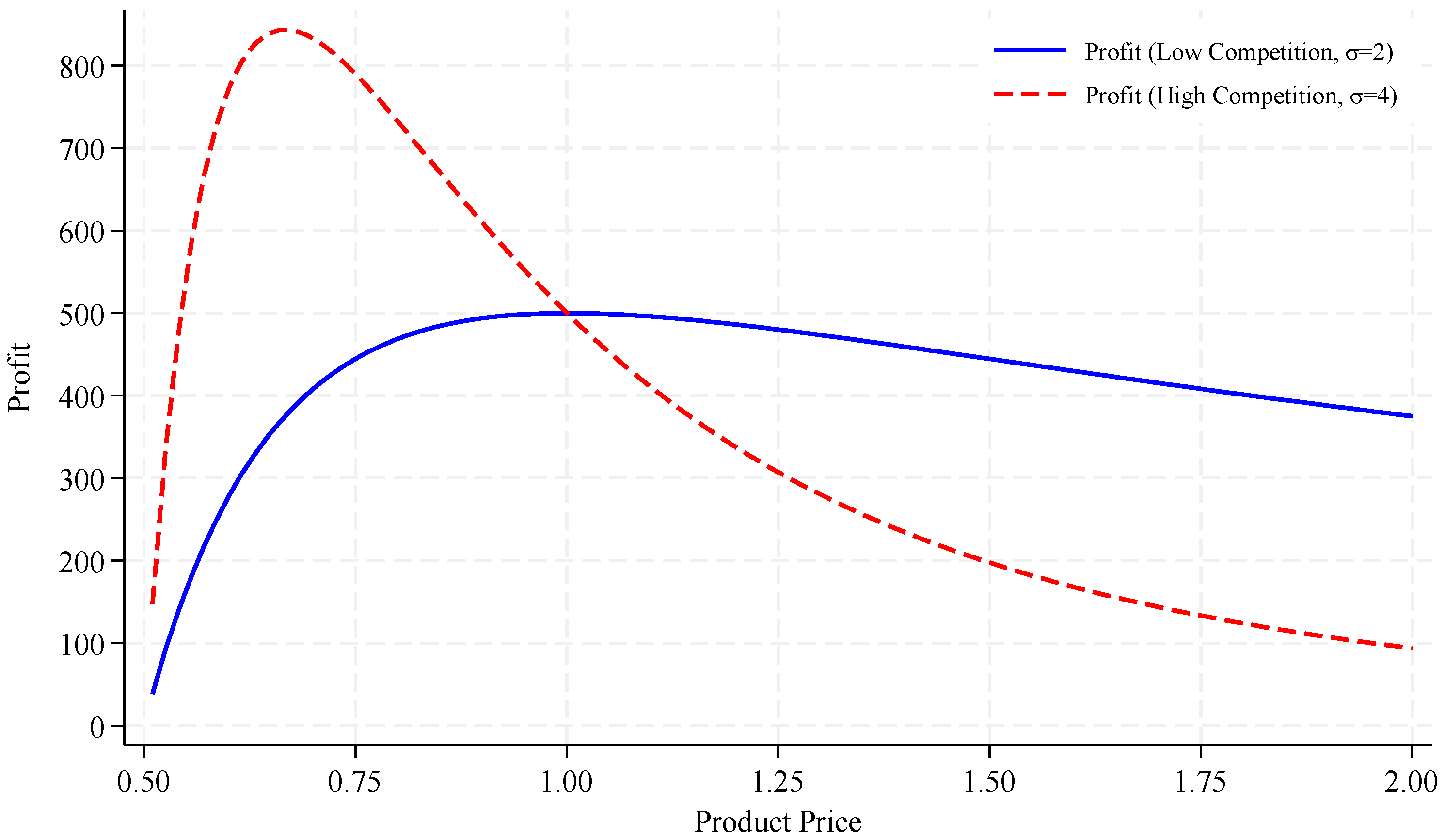
Figure 1 clearly illustrates this proposition, showing that in highly competitive markets, firms that can achieve low costs through increased productivity and effectively implement a low-margin, high-volume strategy will rapidly gain dominance, accumulate more profits and market share, and thus further solidify their competitive advantage. Therefore, when formulating pricing strategies, firms must thoroughly analyze the degree of competition in their market (i.e., the value of $\sigma$). In a highly competitive environment, blindly pursuing high prices may lead to a double loss of market share and profits. Consequently, investing in productivity improvement is fundamental for enterprises, as it provides the cost basis for executing a low-margin, high-volume strategy.

3. Long-Term Profit, Entry Barriers, and Market Structure Evolution

3.1. Strategic Value of Market Share

To further demonstrate the importance of market share to enterprises, we introduce a dynamic competition model. Consider an enterprise’s market share at time t as S_t, and its productivity as A_t. According to Arrow’s (1962) research, the growth of an enterprise’s productivity is positively correlated with cumulative output [31]. Therefore, we assume the productivity growth rate is as follows:

$${\displaystyle \frac{d{A}_t}{dt}}=\beta Q_t{A}_t^{{\alpha }_A}$$

The reason for setting this function is that the more cumulative production experience gained, the faster the production efficiency improves, but with diminishing marginal returns.

Since $Q_t=s_t{Q}_t^{market}$, where $s_t$ is the firm’s sales and $Q_t^{market}$ is the total market demand, we get

$${\displaystyle \frac{d{A}_t}{dt}}=\beta s_t{Q}_t^{market}{A}_t^{{\alpha }_A}$$

Assuming total market demand is stable, i.e., $Q_t^{market}=\overline{Q}$, then we get

$${\displaystyle \frac{A_t^{1-{\alpha }_A}-A_0^{1-{\alpha }_A}}{1-{\alpha }_A}}=\beta \overline{Q}{\displaystyle {\int }_0^t{s}_{\tau }}d\tau$$

Assuming market share is relatively stable in the short term, i.e., $s_t\approx s$, then we get

$$A_t={\left[A_0^{1-{\alpha }_A}+\left(1-{\alpha }_A\right)\beta \overline{Q}{s}_t\right]}^{{\displaystyle \frac{1}{1-{\alpha }_A}}}$$

(12)

In Equation (12), $A_t$ denotes the firm’s total factor or specific factor effective productivity at time t; $A_0$ is the productivity base when the firm enters the market or at the initial observation point (t = 0), reflecting the firm’s inherent endowment or initial technological investment. $\overline{Q}$ is the steady state total market demand, representing the total quantity of products that the entire industry or market can absorb. $\beta$ ($\beta >0$) is the learning efficiency parameter, measuring the firm’s technology conversion rate that translates accumulated production experience (output) into actual productivity gains; it represents the firm’s endogenous learning conversion efficiency, and its magnitude reflects the industry’s technological characteristics of learning by doing. ${\alpha }_A\in \left(0,1\right)$ is the marginal return parameter of learning, which characterizes the degree to which the firm’s productivity growth rate gradually slows down as experience accumulates over the long production process. Now consider two firms: Firm 1 adopts a low-margin, high-volume strategy with an initial market share of $s_1>0.5$; Firm 2 adopts a high-price strategy with an initial market share of $s_2=1-s_1<0.5$. Assume both have the same initial productivity, $A_1\left(0\right)=A_2\left(0\right)=A_0$.

At time t:

$$A_1\left(t\right)={\left[A_0^{1-{\alpha }_A}+\left(1-{\alpha }_A\right)\beta \overline{Q}{s}_{1}t\right]}^{{\displaystyle \frac{1}{1-{\alpha }_A}}}$$

$$A_2\left(t\right)={\left[A_0^{1-{\alpha }_A}+\left(1-{\alpha }_A\right)\beta \overline{Q}{s}_{2}t\right]}^{{\displaystyle \frac{1}{1-{\alpha }_A}}}$$

Calculate the productivity ratio as follows:

$${\displaystyle \frac{A_1\left(t\right)}{A_2\left(t\right)}}={\left[{\displaystyle \frac{A_0^{1-{\alpha }_A}+\left(1-{\alpha }_A\right)\beta \overline{Q}{s}_{1}t}{A_0^{1-{\alpha }_A}+\left(1-{\alpha }_A\right)\beta \overline{Q}{s}_{2}t}}\right]}^{{\displaystyle \frac{1}{1-{\alpha }_A}}}$$

when $t\to \infty$:

$$\underset{t\to \infty }{\lim }{\displaystyle \frac{A_1\left(t\right)}{A_2\left(t\right)}}={\left({\displaystyle \frac{s_1}{s_2}}\right)}^{{\displaystyle \frac{1}{1-{\alpha }_A}}}>1$$

As the productivity gap widens, according to the market share formula (8), we get

$$s_1\left(t\right)={\displaystyle \frac{A_1{\left(t\right)}^{\sigma -1}}{A_1{\left(t\right)}^{\sigma -1}+A_2{\left(t\right)}^{\sigma -1}}}$$

Differentiating $s_1\left(t\right)$ with respect to t, we get

$${\displaystyle \frac{d{s}_1}{dt}}={\displaystyle \frac{\left(\sigma -1\right)A_1^{\sigma -2}\frac{d{A}_1}{dt}\cdot A_2^{\sigma -1}-A_1^{\sigma -1}\left(\sigma -1\right)A_2^{\sigma -2}\frac{d{A}_2}{dt}}{{\left(A_1^{\sigma -1}+A_2^{\sigma -1}\right)}^2}}$$

Since ${\displaystyle \frac{d{A}_1}{dt}}=\beta \overline{Q}{s}_1{A}_1^{{\alpha }_A}$ and ${\displaystyle \frac{d{A}_2}{dt}}=\beta \overline{Q}{s}_2{A}_2^{{\alpha }_A}$, and $s_1>s_2$, it can be proven that

$${\displaystyle \frac{d{s}_1}{dt}}>0$$

(13)

Equation (13) indicates that the initial market share advantage will amplify over time. From Equations (12) and (13), Proposition 2 can be derived.

Proposition 2.

The higher the market share, the faster the productivity growth, and the initial market share advantage will amplify over time.

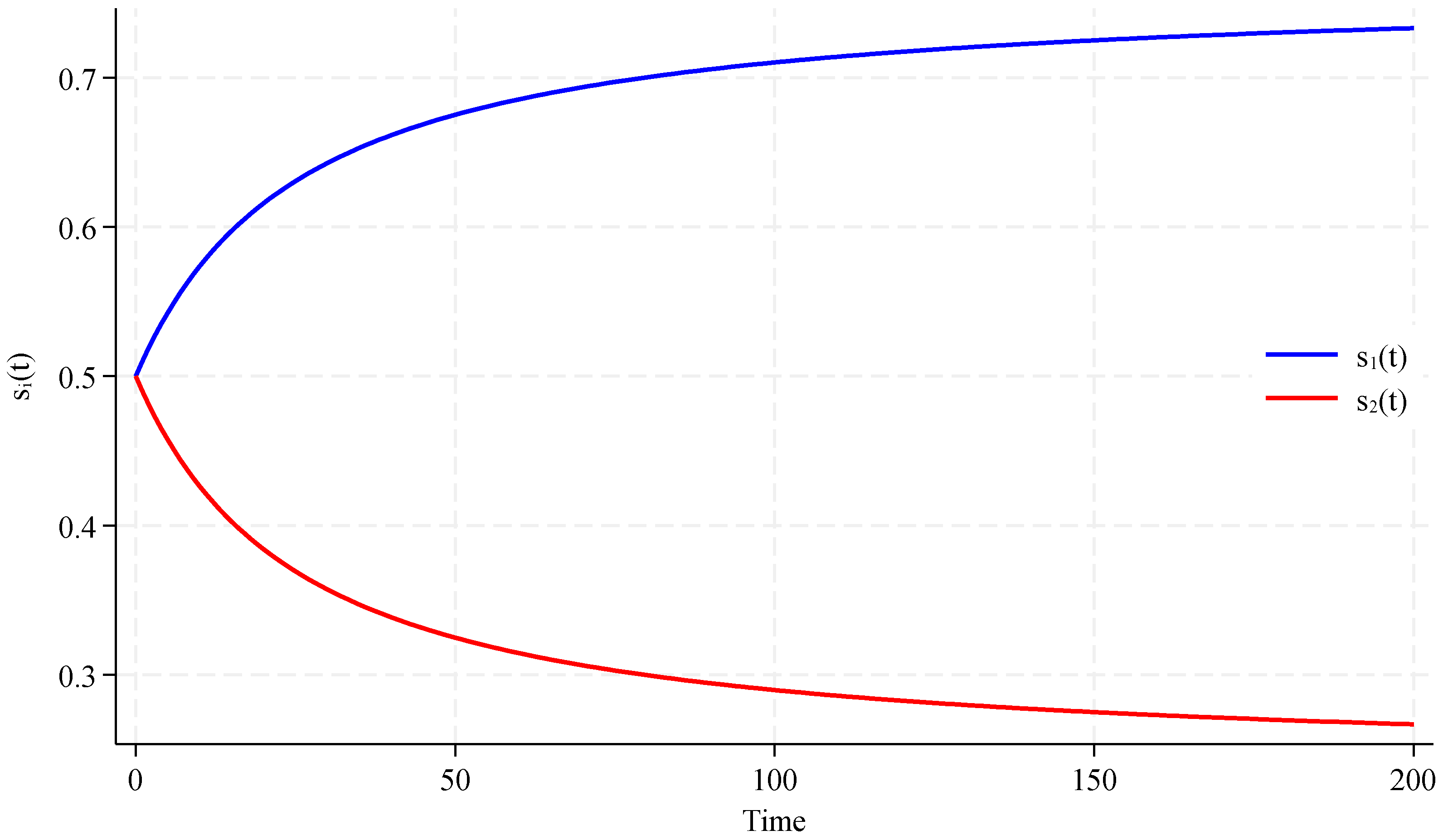
Figure 2 numerically simulates the evolution of market shares of two firms over time. Initially, Firm 1 has a higher market share, $s_1\left(0\right)>s_2\left(0\right)$. According to the theorem’s assumption, as time progresses, the firm with the higher market share will achieve faster growth due to its productivity advantage. Consequently, $s_1\left(t\right)$ monotonically increases and gradually approaches its upper limit, while Firm 2’s market share continuously decreases and converges to a lower level. Therefore, a higher initial productivity leads to an increase in market share, and an expanded market share, in turn, promotes productivity improvement, thereby forming a continuously expanding competitive advantage.

3.2. Cumulative Effects and Entrenched Competitive Advantage

Furthermore, we analyze the cumulative effects of firm profits. Assume that the cumulative profit of firm i within time $\left[0,T\right]$ is as follows:

$${\Pi }_i\left(T\right)={\displaystyle {\int }_0^T\exp }\left(-rt\right){\pi }_i\left(t\right)dt$$

where r is the discount rate. Substituting the profit function (12) into this, we obtain a new profit function:

$${\pi }_i\left(t\right)={\displaystyle \frac{\left(\mu -1\right)M{A}_i{\left(t\right)}^{\sigma -1}}{{\left(\mu \theta \right)}^{\sigma -1}\left[A_1{\left(t\right)}^{\sigma -1}+A_2{\left(t\right)}^{\sigma -1}\right]}}$$

For Firm 1, which adopts a low-price strategy, the cumulative profit function is as follows:

$${\Pi }_1\left(T\right)={\displaystyle {\int }_0^T\exp }\left(-rt\right){\displaystyle \frac{\left(\mu -1\right)M{A}_1{\left(t\right)}^{\sigma -1}}{{\left(\mu \theta \right)}^{\sigma -1}\left[A_1{\left(t\right)}^{\sigma -1}+A_2{\left(t\right)}^{\sigma -1}\right]}}dt$$

The cumulative profit function for Firm 2, which adopts a high-price strategy, is as follows:

$${\Pi }_2\left(T\right)={\displaystyle {\int }_0^T\exp }\left(-rt\right){\displaystyle \frac{\left(\mu -1\right)M{A}_2{\left(t\right)}^{\sigma -1}}{{\left(\mu \theta \right)}^{\sigma -1}\left[A_1{\left(t\right)}^{\sigma -1}+A_2{\left(t\right)}^{\sigma -1}\right]}}dt$$

Then, the cumulative profit ratio can be expressed by the following formula:

$${\displaystyle \frac{{\Pi }_1\left(T\right)}{{\Pi }_2\left(T\right)}}={\displaystyle \frac{{\displaystyle {\int }_0^T\exp }\left(-rt\right)A_1{\left(t\right)}^{\sigma -1}dt}{{\displaystyle {\int }_0^T\exp }\left(-rt\right)A_2{\left(t\right)}^{\sigma -1}dt}}$$

Since $A_1\left(t\right)>A_2\left(t\right)$ holds for all $t>0$, and the gap widens over time, therefore

$${\displaystyle \frac{{\Pi }_1\left(T\right)}{{\Pi }_2\left(T\right)}}>{\left({\displaystyle \frac{A_1\left(0\right)}{A_2\left(0\right)}}\right)}^{\sigma -1}=1$$

More importantly, when $T\to \infty$, this ratio approaches infinity:

$$\underset{T\to \infty }{\lim }{\displaystyle \frac{{\Pi }_1\left(T\right)}{{\Pi }_2\left(T\right)}}=\infty$$

(14)

Equation (14) indicates that in long-term competition, a high-volume, low-margin strategy, through the accumulation of market share advantage, can gain an overwhelming competitive advantage.

3.3. Entry Barriers and Market Structure Evolution

Based on the above analysis, we can further deduce the evolutionary patterns of market structure. Consider a potential entrant, whose entry into the market requires a fixed cost F. After entry, the new firm’s initial productivity is $A_E$.

The condition for the new firm to be profitable is that its expected present value of profits is greater than the entry cost:

$${\displaystyle {\int }_0^T\exp }\left(-rt\right){\pi }_E(t)dt>F$$

Since the incumbent firm (adopting a high-volume, low-margin strategy) has already established a high market share and high productivity advantage, the new firm’s initial market share is very small, i.e.,

$$s_E\left(0\right)={\displaystyle \frac{A_E^{\sigma -1}}{A_1^{\sigma -1}+A_E^{\sigma -1}}}\approx {\displaystyle \frac{A_E^{\sigma -1}}{A_1^{\sigma -1}}}={\left({\displaystyle \frac{A_E}{A_1}}\right)}^{\sigma -1}$$

If $A_1>A_E$, then the new firm’s initial profit is as follows:

$${\pi }_E\left(0\right)={\displaystyle \frac{\left(\mu -1\right)M{A}_E^{\sigma -1}}{{\left(\mu \theta \right)}^{\sigma -1}\left(A_1^{\sigma -1}+A_E^{\sigma -1}\right)}}<{\displaystyle \frac{\left(\mu -1\right)M}{{\left(\mu \theta \right)}^{\sigma -1}}}\cdot {\displaystyle \frac{A_E^{\sigma -1}}{A_1^{\sigma -1}}}$$

Since the new firm’s market share is small and its learning effect is slow, its productivity growth rate is as follows:

$${\displaystyle \frac{d{A}_E}{dt}}=\beta \overline{Q}{s}_E{A}_E^{{\alpha }_A}<\beta \overline{Q}{s}_1{A}_1^{{\alpha }_A}={\displaystyle \frac{d{A}_1}{dt}}$$

This implies that the productivity gap continues to widen, making it difficult for new entrants to catch up with incumbent firms. Specifically, let us calculate the entry condition:

$${\displaystyle {\int }_0^{\infty }\exp }\left(-rt\right){\displaystyle \frac{\left(\mu -1\right)M{A}_E^{\sigma -1}}{{\left(\mu \theta \right)}^{\sigma -1}\left(A_1^{\sigma -1}+A_E^{\sigma -1}\right)}}dt>F$$

(15)

Since $A_1$ grows faster than $A_E$, the value of the above integral decreases over time. Define the critical productivity $A_E^{*}$ such that the entry condition just satisfies equality. Then, when the incumbent firm’s productivity reaches $A_1>A_E^{*}$, the market closes to new entrants, forming a natural monopoly or oligopoly. From Equations (14) and (15), Proposition 3 can be derived.

Proposition 3.

In long-term competition, a high-volume, low-margin strategy gains an overwhelming competitive advantage through market share dominance, thereby building entry barriers and solidifying its market position.

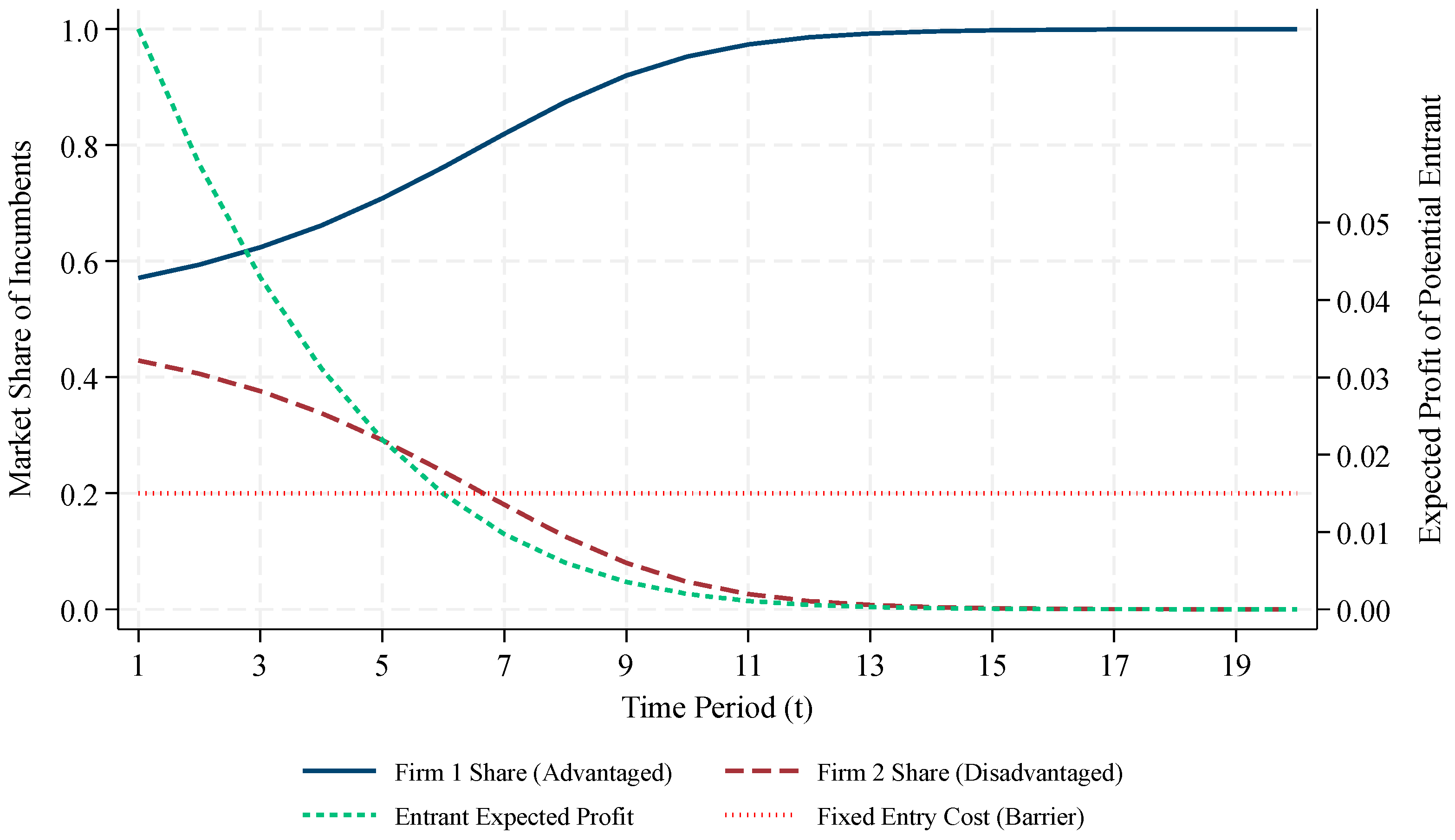
Figure 3 clearly illustrates Proposition 3, revealing two core conclusions: First, over time, Firm 1, with an initial slight advantage, gains more market share and subsequently achieves faster productivity iteration through dynamic learning mechanisms. The two market share evolution curves show a significant “scissor difference” pattern, with Firm 1’s market share asymptotically approaching a monopoly level, while Firm 2 is gradually marginalized ($s_2\to 0$). Second, the expected profit curve of potential entrants (${\pi }_E$) in the figure shows an exponential decay over time. As the productivity of the incumbent advantageous firm (Firm 1) continuously breaks through, the market’s competitive potential rises sharply, and the central product price shifts downward. For potential entrants with ordinary initial productivity, the remaining market demand they can capture shrinks dramatically. When the evolution reaches period $t^{*}$, the potential entrant’s expected profit has fallen below the fixed entry cost line (${\pi }_E<F$), marking the formal formation of insurmountable endogenous entry barriers. This simulation result rigorously demonstrates the scientific validity of Proposition 3 from a mathematical evolutionary logic perspective; that is, in a highly competitive market, early cost advantages not only determine current profits but also determine the long-term market structure and industry moats.

4. Robot Applications and Market Competition

4.1. Labor Substitution Effect of Robots

Currently, production-side robots have become the third factor of production, in addition to labor and capital. Therefore, this section expands upon the basic framework established previously by considering firms introducing robots as a new factor of production. According to Acemoglu and Restrepo (2018) [9,10], robots can be regarded as a special type of capital good, but their substitutability with human labor is more direct. Therefore, we extend the production function to a nested CES production function incorporating three factors: physical capital (K), human labor (L), and robots (R).

$$Q=A{\left\{{\alpha }_1{K}^{-{\rho }_1}+{\alpha }_2{\left[\beta L^{-{\rho }_2}+\left(1-\beta \right)R^{-{\rho }_2}\right]}^{{\displaystyle \frac{{\rho }_1}{{\rho }_2}}}\right\}}^{-{\displaystyle \frac{\nu }{{\rho }_1}}}$$

(16)

where ${\alpha }_1$ measures the relative importance or weight of physical capital (K) in total output. ${\alpha }_2$ measures the relative importance of the composite input consisting of human labor and robots in total output. ${\rho }_1$ is the outer substitution parameter, which determines the elasticity of substitution between physical capital and the “labor-robot” composite input. ${\rho }_2$ is the inner substitution parameter, which determines the direct elasticity of substitution between human labor (L) and robots (R). ν is the returns-to-scale parameter. When $v=1$, it indicates constant returns to scale. $v>1$ or $v<1$ represents increasing or decreasing returns to scale, respectively.

Define comprehensive labor input:

$$\tilde{L}={\left[\beta L^{-{\rho }_2}+\left(1-\beta \right)R^{-{\rho }_2}\right]}^{-{\displaystyle \frac{1}{{\rho }_2}}}$$

(17)

Then the production function can be rewritten as follows:

$$Q=A{\left\{{\alpha }_1{K}^{-{\rho }_1}+{\alpha }_2{\tilde{L}}^{-{\rho }_1}\right\}}^{-{\displaystyle \frac{\nu }{{\rho }_1}}}$$

(18)

Assume the factor prices faced by the enterprise are: physical capital rental $r$, human labor wage $w$, and robot usage cost $w_R$. The costs of a robot include initial purchase cost, maintenance cost, energy cost, and depreciation. Let the robot purchase price be $P_R$ and its service life be $T_R$ years. Then the annualized cost for the enterprise is as follows:

$$w_R={\displaystyle \frac{P_R}{T_R}}\left(1+r\right)+m+e$$

(19)

Among them, m is the maintenance cost rate, and e is the unit energy cost. In contrast, labor costs $w$, including wages, social security, and benefits, are typically rigid and increase over time.

Assume

$$w_R={\theta }_{R}w$$

where ${\theta }_R$ is the robot cost coefficient. Although the initial investment in robots is substantial, the annualized cost is generally lower than that of human labor, especially in developed countries and regions with higher labor costs. Therefore, we set ${\theta }_R<1$.

Thus, by minimizing the firm’s cost at a given output level, we can derive the following:

$${\displaystyle \frac{L}{R}}={\left({\displaystyle \frac{\beta }{1-\beta }}\cdot {\theta }_R\right)}^{{\displaystyle \frac{1}{1+{\rho }_2}}}={\left({\displaystyle \frac{\beta {\theta }_R}{1-\beta }}\right)}^{{\displaystyle \frac{1}{1+{\rho }_2}}}={\left({\displaystyle \frac{\beta {\theta }_R}{1-\beta }}\right)}^{{\sigma }_2}$$

(20)

where ${\sigma }_2={\displaystyle \frac{1}{1+{\rho }_2}}$ is the elasticity of substitution between labor and robots.

Substituting Equation (20) into Equation (17), we can obtain the following:

$$L=\tilde{L}{\left[\beta +\left(1-\beta \right){\left({\displaystyle \frac{R}{L}}\right)}^{-{\rho }_2}\right]}^{-{\displaystyle \frac{1}{{\rho }_2}}}$$

(21)

$$R=\tilde{L}{\left[\beta {\left({\displaystyle \frac{L}{R}}\right)}^{-{\rho }_2}+\left(1-\beta \right)\right]}^{-{\displaystyle \frac{1}{{\rho }_2}}}$$

(22)

Substituting Equation (20) into Equations (21) and (22), we can obtain the minimum cost of composite labor:

$$C_{\tilde{L}}=wL+w_{R}R=\tilde{L}w{\left[{\beta }^{{\sigma }_2}{\theta }_R^{{\sigma }_2-1}+{\left(1-\beta \right)}^{{\sigma }_2}{\theta }_R^{{\sigma }_2}\right]}^{{\displaystyle \frac{1}{{\sigma }_2}}}$$

Define the effective price of composite labor:

$$\tilde{w}=w{\left[{\beta }^{{\sigma }_2}{\theta }_R^{{\sigma }_2-1}+{\left(1-\beta \right)}^{{\sigma }_2}{\theta }_R^{{\sigma }_2}\right]}^{{\displaystyle \frac{1}{{\sigma }_2}}}$$

(23)

Then the cost of composite labor is $C_{\tilde{L}}=\tilde{w}\tilde{L}$.

4.2. Impact of Robot Substitution on Total Cost

Given output $Q$, the firm chooses physical capital K and composite labor $\tilde{L}$ to minimize total cost:

$$\underset{K,L}{\min }rK+\tilde{w}\tilde{L}$$

$$s.t. A{\left[{\alpha }_1{K}^{-{\rho }_1}+{\alpha }_2{\tilde{L}}^{-{\rho }_1}\right]}^{-{\displaystyle \frac{\nu }{{\rho }_1}}}=Q$$

When there are constant returns to scale ($\nu =1$), the unit cost is as follows:

$$c={\left[{\alpha }_1^{{\sigma }_1}{r}^{1-{\sigma }_1}+{\alpha }_2^{{\sigma }_1}{\tilde{w}}^{1-{\sigma }_1}\right]}^{{\displaystyle \frac{1}{1-{\sigma }_1}}}\cdot A^{-1}$$

(24)

where ${\sigma }_1={\displaystyle \frac{1}{1+{\rho }_1}}$ is the capital–labor elasticity of substitution.

Substituting Equation (23) into Equation (24) yields:

$$c=A^{-1}\cdot {\left[{\alpha }_1^{{\sigma }_1}{r}^{1-{\sigma }_1}+{\alpha }_2^{{\sigma }_1}{w}^{1-{\sigma }_1}{\left[{\beta }^{{\sigma }_2}{\theta }_R^{{\sigma }_2-1}+{\left(1-\beta \right)}^{{\sigma }_2}{\theta }_R^{{\sigma }_2}\right]}^{{\displaystyle \frac{1-{\sigma }_1}{{\sigma }_2}}}\right]}^{{\displaystyle \frac{1}{1-{\sigma }_1}}}$$

(25)

Taking the partial derivative of Equation (25) with respect to ${\theta }_R$ yields:

$$\begin{array}{c}{\displaystyle \frac{\mathsf{\partial }c}{\mathsf{\partial }{\theta }_R}}=A^{-1}\cdot {\alpha }_2^{{\sigma }_1}{w}^{1-{\sigma }_1}\cdot {\displaystyle \frac{1-{\sigma }_1}{{\sigma }_2}}{\left[{\beta }^{{\sigma }_2}{\theta }_R^{{\sigma }_2-1}+{\left(1-\beta \right)}^{{\sigma }_2}{\theta }_R^{{\sigma }_2}\right]}^{{\displaystyle \frac{1-{\sigma }_1}{{\sigma }_2}}-1}\\ \cdot \left[{\beta }^{{\sigma }_2}\left({\sigma }_2-1\right){\theta }_R^{{\sigma }_2-2}+{\left(1-\beta \right)}^{{\sigma }_2}{\sigma }_2{\theta }_R^{{\sigma }_2-1}\right]>0\end{array}$$

(26)

Equation (26) shows that a decrease in the robot cost coefficient ${\theta }_R$ will lead to a decrease in the firm’s unit production cost c.

4.3. Dynamic Feedback Effects: Economies of Scale and Learning Curve

Whether a firm adopts robots depends on cost comparison. Assume the cost for a firm not using robots is $c_0$. If the firm invests in purchasing robots, it needs to pay a fixed cost $F_R$, and the cost after using robots is $c_R$. Therefore, the cost saving rate is as follows:

$$\Delta c={\displaystyle \frac{c_0-c_R}{c_0}}$$

The net present value for a firm adopting robots is as follows:

$$NP{V}_R={\displaystyle {\int }_0^{\infty }\exp \left(-rt\right)}\left(c_0-c_R\right)Qdt-F_R$$

Assuming stable output, $Q_t=\overline{Q}$, then

$$NP{V}_R={\displaystyle \frac{\left(c_0-c_R\right)\overline{Q}}{r}}-F_R$$

The condition for a firm to adopt robots is $NP{V}_R>0$, which means that

$$\overline{Q}>{\displaystyle \frac{r{F}_R}{\left(c_0-c_R\right)}}={\displaystyle \frac{r{F}_R}{c_0\Delta c}}$$

From this, the critical output for using robots can be derived as follows:

$${\overline{Q}}^{*}={\displaystyle \frac{r{F}_R}{c_0\Delta c}}$$

(27)

Equation (27) indicates that only firms whose output exceeds the critical value will adopt robots. The critical value is inversely proportional to the cost saving rate $\Delta c$, meaning the greater the cost saving, the lower the critical output, and more firms will adopt robots.

Assuming the firm’s output follows the distribution function $G\left(Q\right)$, the proportion of firms adopting robots is:

$${\pi }_R=1-G\left({\overline{Q}}^{*}\right)=1-G\left({\displaystyle \frac{r{F}_R}{c_0\Delta c}}\right)$$

Taking the derivative with respect to ${\theta }_R$ yields:

$${\displaystyle \frac{\mathsf{\partial }{\pi }_R}{\mathsf{\partial }{\theta }_R}}=-g\left({\overline{Q}}^{*}\right)\cdot {\displaystyle \frac{\mathsf{\partial }{\overline{Q}}^{*}}{\mathsf{\partial }{\theta }_R}}$$

where

$${\displaystyle \frac{\mathsf{\partial }{\overline{Q}}^{*}}{\mathsf{\partial }{\theta }_R}}=-{\displaystyle \frac{r{F}_R}{c_0\Delta c^2}}\cdot {\displaystyle \frac{\mathsf{\partial }\Delta c}{\mathsf{\partial }{\theta }_R}}>0$$

Since $\Delta c$ is a decreasing function of ${\theta }_R$, it follows that ${\displaystyle \frac{\mathsf{\partial }{\pi }_R}{\mathsf{\partial }{\theta }_R}}<0$. This implies that a decrease in robot costs will increase the industry’s robot adoption rate.

Drawing on learning curve theory, an increase in cumulative production reduces the unit cost. Assume the price of robots is as follows:

$$P_R\left(t\right)=P_R\left(0\right)\cdot {\left[{\displaystyle \sum _{s=0}^t{Q}_R\left(s\right)}\right]}^{-\lambda }$$

where $Q_R\left(s\right)$ is the robot output at time s, and $\lambda >0$ is the learning parameter.

Robot output depends on demand, and demand comes from the number and scale of firms adopting robots:

$$Q_R\left(t\right)={\displaystyle {\int }_{{\overline{Q}}^{*}\left(t\right)}^{\infty }R\left(Q\right)}\cdot g\left(Q\right)dQ$$

where $R\left(Q\right)$ is the amount of robots used by a firm with product output $Q$.

This forms a positive feedback loop: a decrease in robot price ($P_R$) leads to a decrease in the robot cost coefficient (${\theta }_R$), which in turn leads more firms to adopt robots (${\pi }_R$). This increases robot output ($Q_R$), further driving down robot prices ($P_R$). This cycle can be expressed by the iterative equation:

$${\theta }_R\left(t+1\right)={\theta }_R\left(t\right)\cdot {\left[1+\lambda \ln \left({\displaystyle \frac{Q_R\left(t\right)}{Q_R\left(t-1\right)}}\right)\right]}^{-1}$$

(28)

As $Q_R$ continues to grow, ${\theta }_R$ continues to decrease until it reaches the technological frontier.

Defining the growth rate of robot adoption as $g_{\pi }={\displaystyle \frac{d{\pi }_R}{dt}}$, it can be written in the following form:

$$g_{\pi }={\displaystyle \frac{d{\pi }_R}{d{\theta }_R}}\cdot {\displaystyle \frac{d{\theta }_R}{dt}}$$

Since ${\displaystyle \frac{d{\theta }_R}{dt}}\propto -Q_R$, and $Q_R\propto {\pi }_R$, thus $g_{\pi }\propto {\pi }_R$; at the same time, there is an upper limit ${\pi }_R\le 1$, so

$${\displaystyle \frac{d{\pi }_R}{dt}}=k{\pi }_R\left(1-{\pi }_R\right)$$

(29)

This is a logistic differential equation; solving it yields:

$$t^{*}={\displaystyle \frac{1}{k}}\ln \left({\displaystyle \frac{1-{\pi }_0}{{\pi }_0}}\right)$$

(30)

$${\displaystyle \frac{d{\pi }_R/dt}{{\pi }_R}}=k\left(1-{\pi }_R\right)$$

(31)

From Equation (31), when ${\pi }_R$ is small, the growth rate approaches k; when ${\pi }_R$ approaches 1, the growth rate tends to 0; when ${\pi }_R$ = 0.5, the growth rate is 0.5 k, and the absolute growth rate is maximized. Therefore, the growth rate accelerates when ${\pi }_R$ < 0.5 and decelerates when ${\pi }_R$ > 0.5. The inflection point is at ${\pi }_R$ = 0.5. This indicates that robot adoption exhibits an S-shaped curve phenomenon of technology diffusion, meaning slow growth in the initial stage, accelerated growth in the middle stage, and saturation in the later stage.

Assume that with continuous technological progress, the cost of robots continuously decreases exponentially, i.e.,

$${\theta }_R\left(t\right)={\theta }_R^0\exp \left(-\lambda t\right)$$

And the diffusion speed is affected by

$$k\left(t\right)=k_0+\beta \left[{\theta }_R^0-{\theta }_R\left(t\right)\right]=k_0+\beta {\theta }_R^0\left[1-\exp \left(-\lambda t\right)\right]$$

The modified equation for (32) is as follows:

$${\displaystyle \frac{d{\pi }_R}{dt}}=\left\{k_0+\beta {\theta }_R^0\left[1-\exp \left(-\lambda t\right)\right]\right\}\cdot {\pi }_R\left(1-{\pi }_R\right)$$

Let $K\left(t\right)={\displaystyle {\int }_0^{t}k\left(s\right)}ds=k_{0}t+\beta {\theta }_R^0\left\{t+{\displaystyle \frac{1}{\lambda }}\left[\exp \left(-\lambda t\right)-1\right]\right\}$, we can obtain

$${\pi }_R\approx {\displaystyle \frac{1}{1+\left(\frac{1-{\pi }_0}{{\pi }_0}\right)\exp \left(-K\left(t\right)\right)}}$$

(32)

Furthermore, we can deduce that

$$\underset{t\to \infty }{\lim }K\left(t\right)=\infty \Rightarrow \underset{t\to \infty }{\lim }{\pi }_R\left(t\right)=1$$

(33)

Equation (33) shows that for smaller $t$, $K\left(t\right)\approx k_{0}t$, and the robot adoption rate resembles a standard S-curve. After t increases to a certain extent, the growth rate of $K\left(t\right)$ accelerates, making the growth in the intermediate stage steeper. As t continues to increase, the stage that should have saturated will experience a significantly prolonged saturation time due to the continuous increase in $K\left(t\right)$.

From Equations (31)–(33), Proposition 4 can be derived.

Proposition 4.

Robot adoption exhibits an S-shaped curve phenomenon of technological diffusion, characterized by slow initial growth, accelerated middle-stage growth, and late-stage saturation. However, technological advancement makes the middle-stage growth steeper and significantly prolongs the time to reach saturation.

The “prolonged saturation + steeper middle-stage” of robot adoption signifies that society has lost its “golden adaptation window.” Ostensibly, there appears to be ample preparation time, but in reality, the impact will erupt intensively within a very short period. It is like a frog slowly boiled in warm water, suddenly finding itself in boiling water; by the time you realize the severity, it is too late to react. Even worse, just when one might expect to enter a stable period after enduring this wave of impact, continuous technological upgrades lead to ceaseless disruptions. This compels workers to constantly learn new skills throughout their lives, traps businesses in short-term decision-making, leaves government policies perpetually lagging, and continuously widens social inequality. This is no longer a “one-time technological transformation pain” but has evolved into a “permanent adaptation crisis,” fundamentally challenging the traditional economic assumption that “markets will automatically adjust to a new equilibrium.”

4.4. Robot Adoption and Market Share

Now consider the heterogeneity of firm productivity [40,41]. Assume that the total factor productivity $A_i$ of firms follows a distribution $F\left(A\right)$, with density function $f\left(A\right)$.

For a firm with productivity A, its cost is

$$c\left(A,{\theta }_R\right)={\displaystyle \frac{1}{A}}{\left[{\alpha }_1^{{\sigma }_1}{r}^{1-{\sigma }_1}+{\alpha }_2^{{\sigma }_1}{w}^{1-{\sigma }_1}{\left[{\beta }^{{\sigma }_2}{\theta }_R^{{\sigma }_2-1}+{\left(1-\beta \right)}^{{\sigma }_2}{\theta }_R^{{\sigma }_2}\right]}^{{\displaystyle \frac{1-{\sigma }_1}{{\sigma }_2}}}\right]}^{{\displaystyle \frac{1}{1-{\sigma }_1}}}$$

After adopting robots, effective productivity improves. Let the adoption of robots increase effective productivity from A to $\tilde{A}$, where the increase is as follows:

$$\tilde{A}=A\cdot \varphi \left({\theta }_R\right)$$

Here, $\varphi \left({\theta }_R\right)$ is the efficiency gain coefficient. According to the cost-productivity relationship $c={\displaystyle \frac{\theta }{A}}$ (assuming constant returns to scale), we have

$${\displaystyle \frac{c\left(A,{\theta }_R\right)}{c\left(A,1\right)}}={\displaystyle \frac{\tilde{A}}{A}}$$

Therefore,

$$\varphi \left({\theta }_R\right)={\displaystyle \frac{c\left(A,1\right)}{c\left(A,{\theta }_R\right)}}={\displaystyle \frac{1}{1-\Delta c}}$$

The market share of firms adopting robots is as follows:

$$s_i^R={\displaystyle \frac{{\left[\varphi \left({\theta }_R\right)A_i\right]}^{\sigma -1}}{{\displaystyle {\sum }_{A_j<A^{*}}{A}_j^{\sigma -1}+{\displaystyle {\sum }_{A_k\ge A^{*}}{\left[\varphi \left({\theta }_R\right)A_k\right]}^{\sigma -1}}}}}$$

The market share of firms not adopting robots is as follows:

$$s_i^{NR}={\displaystyle \frac{A_i^{\sigma -1}}{{\displaystyle {\sum }_{A_j<A^{*}}{A}_j^{\sigma -1}+{\displaystyle {\sum }_{A_k\ge A^{*}}{\left[\varphi \left({\theta }_R\right)A_k\right]}^{\sigma -1}}}}}$$

Calculate market share ratio:

$${\displaystyle \frac{s_i^R}{s_i^{NR}}}=\varphi {\left({\theta }_R\right)}^{\sigma -1}={\left({\displaystyle \frac{1}{1-\Delta c}}\right)}^{\sigma -1}$$

(34)

Since $\Delta c$ > 0, we have ${\displaystyle \frac{s_i^R}{s_i^{NR}}}>1$, and this ratio increases with the cost saving rate Δc and with the degree of market competition σ.

Proposition 5 can be derived from Equation (34).

Proposition 5.

Firms adopting robots not only reduce costs but also expand their market share through price advantages, and this market share advantage is amplified in highly competitive markets.

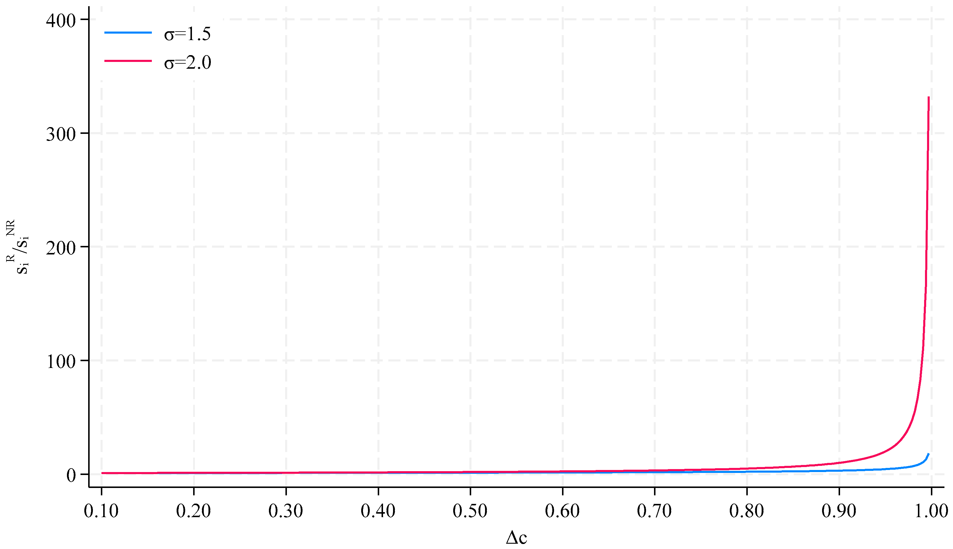
Proposition 5 indicates that an increase in the cost savings rate brought by robots simultaneously leads to higher effective productivity, thereby creating a price advantage under cost-plus pricing. This price advantage is then transformed into a relative expansion of market share through the substitution mechanism of CES demand. Figure 4 shows that as the horizontal axis $\Delta c$ increases, the market share ratio monotonically increases overall and rises sharply as it approaches the upper bound. This suggests that the market share advantage does not accumulate non-linearly but is further amplified in highly competitive environments. Comparing the curves for $\sigma$ = 2.0 and $\sigma$ = 1.5, it can be seen that when the elasticity of substitution is higher, the market share ratio increases more steeply. Therefore, robots not only reduce costs but also strengthen the advantages of leading firms through price-demand substitution-market share mapping, driving the industry towards greater concentration.

5. Conclusions

In this study, a theoretical framework is constructed based on the CES production function and demand structure, with the purpose of deeply analyzing the microeconomic mechanisms behind increasing market concentration and entrenched competitive advantages. By integrating productivity differences, cost-plus pricing, market share, profits, and endogenous learning effects, and specifically considering the substitution of technological factors represented by robotics.

The research findings indicate that, at a static level, the distribution of firm market share and profits is profoundly influenced by relative productivity differences. We demonstrate that highly productive firms, leveraging their cost advantages and optimal cost-plus pricing strategies, can secure larger market shares within a CES demand structure characterized by elasticity of substitution. More importantly, this study reveals a significant asymmetric sensitivity of profits to productivity differences: even a small lead in productivity can be transformed into a disproportionate profit advantage through market competition mechanisms, and this effect is amplified with increased demand elasticity of substitution, thereby accelerating the concentration of profits among a few highly efficient firms.

On the dynamic level, the core contribution of this paper lies in endogenizing the learning effect and transforming static advantages into dynamic competitive advantages. The model clearly demonstrates that market share is not merely a result of performance; rather, it serves as a crucial resource that accelerates firms’ productivity improvements through a “learning by doing” mechanism. This implies that initial market leaders, by virtue of the faster learning speed brought about by their larger market shares, can continuously widen the productivity gap with followers, thereby consistently solidifying their market position.

It is noteworthy that this study specifically investigates the reinforcing role of technological factor substitution, exemplified by robot application, in this process. Robotics, by significantly boosting production efficiency and reducing unit costs, not only statically endows leading firms with stronger cost and price advantages but also dynamically accelerates their learning curves and productivity growth. This accumulation of technological advantages further accelerates the process of increasing market concentration and has a profound impact on the industry structure. Ultimately, due to insufficient market share and lagging learning speeds, potential entrants find the catch-up costs too high and expected returns on investment diminish, thereby endogenously creating barriers to entry for incumbents. These barriers are no longer merely traditional fixed or sunk costs but rather stem from differences in learning capabilities and the solidification of technological advantages in dynamic competition, driving the continuous evolution of industry structure towards high concentration.

The theoretical contributions of this paper are reflected in the following aspects: First, it provides a complete and analytically tractable chain of competitiveness transmission from productivity, costs, pricing, demand, and market share to profits, offering a unified micro-foundation for firm performance heterogeneity. Second, it endogenizes learning effects into a dynamic mechanism closely linked to market share, successfully depicting how static advantages transform into long-term dynamic dominance through positive feedback loops. Third, it deeply analyzes the critical role of technological factor substitution, such as robotics, in accelerating market concentration and solidifying competitive advantages. Finally, by revealing the limited scope for dynamic catch-up, this study endogenously elucidates the formation of entry barriers, providing a new perspective for understanding industry concentration.

The findings of this study offer important policy insights. Based on our theoretical propositions, we suggest that policymakers might consider that, given highly productive firms may continuously accumulate advantages under current market mechanisms, and that technological factor substitution may further accelerate this process, antitrust authorities should closely monitor the dynamic evolution of market concentration and scrutinize potential abuses of market dominance. This could prevent excessive concentration from harming market vitality and innovation. Furthermore, if these theoretical mechanisms hold empirically, it highlights the importance of fostering knowledge spillovers to mitigate monopolistic advantages. Specifically, accompanying policies that encourage technological innovation and talent development in small and medium-sized enterprises (SMEs) may help to weaken the monopolistic learning advantages of leading firms, thereby creating conditions for maintaining a certain dynamism in market competition.

While this study rigorously derives propositions regarding market concentration, technology substitution (such as robotics), and learning-by-doing effects through a CES framework, we acknowledge a significant limitation: the absence of empirical testing. This paper is explicitly framed as a purely theoretical contribution. The analytical results, though mathematically sound, have not yet been validated against real-world firm-level or industry-level data. Testing our theoretical propositions requires highly granular panel data, ideally from the manufacturing or technology sectors, where capital–labor substitution (e.g., robotics adoption) and learning-by-doing effects are most pronounced. Future empirical research is highly encouraged to bridge this gap. For instance, researchers could utilize firm-level panel data to empirically test how initial productivity disparities asymmetrically affect profit margins and market share over time, as proposed in our model. Furthermore, the empirical quantification of the ‘barriers to entry’ generated by these theoretical mechanisms remains a critical next step. By outlining these theoretical mechanisms, we hope to provide a structured roadmap for future empirical scholars to validate, refine, or challenge our findings using econometric analyses.

References

1. Li, M.; Chen, H.; Zhou, G.; Du, D. Time-Dependent Tensor Variational Inequality for an Oligopolistic Market Equilibrium Problem. J. Nonlinear Var. Anal. 2025, 9, 133–160. [Google Scholar] [CrossRef]
2. Bisi, M.; Conte, M.; Groppi, M. Kinetic Modeling of Knowledge and Wealth Dynamics in National and Global Markets. Math. Models Methods Appl. Sci. 2026, 36, 1271–1305. [Google Scholar] [CrossRef]
3. Ounaies, S.; Bonnisseau, J.-M.; Chebbi, S. Equilibrium of a Production Economy with Non-Compact Attainable Allocations Set. Adv. Nonlinear Anal. 2019, 8, 979–994. [Google Scholar] [CrossRef]
4. Rafales, J.; Vazquez, C. Models and Numerical Methods for Equilibrium Problems with Heterogeneous Agents Involving Two Productive Sectors. J. Comput. Appl. Math. 2026, 472, 116812. [Google Scholar] [CrossRef]
5. Baiardi, L.C.; Naimzada, A.K. An Oligopoly Model with Rational and Imitation Rules. Math. Comput. Simul. 2019, 156, 254–278. [Google Scholar] [CrossRef]
6. Takeng, R.T. Uncertain Production Environment and Communication Structure. J. Math. Econ. 2022, 102, 102744. [Google Scholar] [CrossRef]
7. Autor, D.; Autor, D.; Salomons, A.; Salomons, A. Is Automation Labor Share-Displacing? Productivity Growth, Employment, and the Labor Share; National Bureau of Economic Research: Cambridge, MA, USA, 2018; p. w24871. [Google Scholar] [CrossRef]
8. De Loecker, J.; Eeckhout, J.; Unger, G. The Rise of Market Power and the Macroeconomic Implications. Q. J. Econ. 2020, 135, 561–644. [Google Scholar] [CrossRef]
9. Acemoglu, D.; Restrepo, P. The Race between Man and Machine: Implications of Technology for Growth, Factor Shares, and Employment. Am. Econ. Rev. 2018, 108, 1488–1542. [Google Scholar] [CrossRef]
10. Acemoglu, D.; Restrepo, P. Artificial Intelligence, Automation and Work; National Bureau of Economic Research: Cambridge, MA, USA, 2018; p. w24196. [Google Scholar] [CrossRef]
11. Aghion, P.; Howitt, P. A Model of Growth Through Creative Destruction. Econometrica 1992, 60, 323–351. [Google Scholar] [CrossRef]
12. Umar, A.; Shi, Z.; Khlil, A.; Farouk, Z.I.B. Developing a New Robust Swarm-Based Algorithm for Robot Analysis. Mathematics 2020, 8, 158. [Google Scholar] [CrossRef]
13. Zhang, Y. To Enter or Not to Enter? A Competitive Analysis with Minimum Quality Standards. Math. Comput. Simul. 2019, 166, 508–527. [Google Scholar] [CrossRef]
14. Sahu, B.; Das, P.K.; Kabat, M.R. Multi-Robot Co-Operation for Stick Carrying Application Using Hybridization of Meta-Heuristic Algorithm. Math. Comput. Simul. 2022, 195, 197–226. [Google Scholar] [CrossRef]
15. Krakhmalev, O.; Krakhmalev, N.; Gataullin, S.; Makarenko, I.; Nikitin, P.; Serdechnyy, D.; Liang, K.; Korchagin, S. Mathematics Model for 6-DOF Joints Manipulation Robots. Mathematics 2021, 9, 2828. [Google Scholar] [CrossRef]
16. Ochigame, R. Automated Mathematics and the Reconfiguration of Proof and Labor. Bull. Am. Math. Soc. 2024, 61, 423–437. [Google Scholar] [CrossRef]
17. Ren, J.; Sun, H.; Xu, G.; Hou, D. Convergence of Output Dynamics in Duopoly Co-Opetition Model with Incomplete Information. Math. Comput. Simul. 2023, 207, 209–225. [Google Scholar] [CrossRef]
18. Korinek, A.; Vipra, J. Concentrating Intelligence: Scaling and Market Structure in Artificial Intelligence. Econ. Policy 2025, 40, 225–256. [Google Scholar] [CrossRef]
19. Syverson, C. What Determines Productivity? J. Econ. Lit. 2011, 49, 326–365. [Google Scholar] [CrossRef]
20. Bartelsman, E.J.; Doms, M. Understanding Productivity: Lessons from Longitudinal Microdata. J. Econ. Lit. 2000, 38, 569–594. [Google Scholar] [CrossRef]
21. Autor, D.; Dorn, D.; Katz, L.F.; Patterson, C.; Van Reenen, J. The Fall of the Labor Share and the Rise of Superstar Firms. Q. J. Econ. 2020, 135, 645–709. [Google Scholar] [CrossRef]
22. Firooz, H.; Liu, Z.; Wang, Y. Automation and the Rise of Superstar Firms. J. Monet. Econ. 2025, 151, 103733. [Google Scholar] [CrossRef]
23. Dixit, A.K.; Stiglitz, J.E. Monopolistic Competition and Optimum Product Diversity. Am. Econ. Rev. 1977, 67, 297–308. Available online: http://www.jstor.org/stable/1831401 (accessed on 24 May 2026).
24. Passacantando, M.; Raciti, F. A Unified Variational Framework for Global Agricultural Supply Chains Under Uncertain Exchange Rates: New Classes of Cost and Price Functions. J. Nonlinear Var. Anal. 2025, 9, 617–635. [Google Scholar] [CrossRef]
25. Hall, R. The Relation Between Price and Marginal Cost in U.S. Industry; National Bureau of Economic Research: Cambridge, MA, 1986; p. w1785. [Google Scholar] [CrossRef]
26. Graetz, G.; Michaels, G. Robots at Work. Rev. Econ. Stat. 2018, 100, 753–768. [Google Scholar] [CrossRef]
27. Hopenhayn, H.A. Entry, exit, and firm dynamics in long run equilibrium. Econometrica 1992, 60, 1127–1150. [Google Scholar] [CrossRef]
28. Wang, C.-N.; Tibo, H.; Hong, A.N. Malmquist Productivity Analysis of Top Global Automobile Manufacturers. Mathematics 2020, 8, 580. [Google Scholar] [CrossRef]
29. Melitz, M.J. The Impact of Trade on Intra-Industry Reallocations and Aggregate Industry Productivity. Econometrica 2003, 71, 1695–1725. [Google Scholar] [CrossRef]
30. Bajgar, M.; Berlingieri, G.; Calligaris, S.; Criscuolo, C.; Timmis, J. Industry Concentration in Europe and North America. Ind. Corp. Change 2025, 34, 407–424. [Google Scholar] [CrossRef]
31. Arrow, K.J. The Economic Implications of Learning by Doing. In Readings in the Theory of Growth: A Selection of Papers from the Review of Economic Studies; Hahn, F.H., Ed.; Palgrave Macmillan UK: London, UK, 1971; pp. 131–149. ISBN 978-1-349-15430-2. [Google Scholar] [CrossRef]
32. Jovanovic, B.; MacDonald, G.M. The Life Cycle of a Competitive Industry. J. Political Econ. 1994, 102, 322–347. [Google Scholar] [CrossRef]
33. Foster, L.; Haltiwanger, J.; Krizan, C.J. Aggregate Productivity Growth: Lessons from Microeconomic Evidence; National Bureau of Economic Research: Cambridge, MA, USA, 1998; p. w6803. [Google Scholar] [CrossRef]
34. Aghion, P.; Bergeaud, A.; Boppart, T.; Klenow, P.J.; Li, H. A Theory of Falling Growth and Rising Rents. Rev. Econ. Stud. 2023, 90, 2675–2702. [Google Scholar] [CrossRef]
35. Allen, G.I.; Gan, L.; Zheng, L. Interpretable Machine Learning for Discovery: Statistical Challenges and Opportunities. Annu. Rev. Stat. Appl. 2024, 11, 97–121. [Google Scholar] [CrossRef]
36. Tan, L.; Lai, X.; Zhao, Y.; Zhong, Y. Artificial Intelligence and the Emergence of New Quality Productive Forces: A Machine Learning Perspective. Mathematics 2025, 14, 135. [Google Scholar] [CrossRef]
37. Ericson, R.; Pakes, A. Markov-Perfect Industry Dynamics: A Framework for Empirical Work. Rev. Econ. Stud. 1995, 62, 53–82. [Google Scholar] [CrossRef]
38. Zhang, Y.-C. Entry-Exit Decisions with Output Reduction during Exit Periods. AIMS Math. 2024, 9, 6555–6567. [Google Scholar] [CrossRef]
39. Acemoglu, D.; Jensen, M.K. Aggregate Comparative Statics. Games Econ. Behav. 2013, 81, 27–49. [Google Scholar] [CrossRef]
40. Prabakaran, G.; Vaithiyanathan, D.; Ganesan, M. FPGA Based Effective Agriculture Productivity Prediction System Using Fuzzy Support Vector Machine. Math. Comput. Simul. 2021, 185, 1–16. [Google Scholar] [CrossRef]
41. Matsumoto, A.; Szidarovszky, F. Emission Control in an N-Firm Oligopoly Game with Product Differentiation. Mathematics 2025, 13, 2007. [Google Scholar] [CrossRef]
Figure 1. Market competition and the low-margin, high-volume strategy. The horizontal axis is the firm’s product price, which reflects the level of the markup rate, and the vertical axis is the firm’s profit). The peak of the curve represents the optimal pricing that maximizes profit.
Mathematics 14 01892 g001
Figure 2. Time evolution trend of the initial market share advantage. With time t on the horizontal axis and market share on the vertical axis, Enterprise 1 holds a slight advantage in market share at the initial moment.
Mathematics 14 01892 g002
Figure 3. Market advantage of the high-volume, low-margin strategy. The horizontal axis represents time t. The left vertical axis shows the evolution of the incumbent firm’s market share, while the right vertical axis represents the expected profit that a potential entrant can obtain upon entering the market. The horizontal dashed line F denotes the fixed entry cost. When π E < F , an endogenous entry barrier is formally established, and the market closes to new entrants.
Mathematics 14 01892 g003
Figure 4. Relationship between robot cost savings rate and market share. The horizontal axis is the cost saving rate from robot adoption, and the vertical axis is the market share ratio between robot-adopting firms and non-adopting firms.
Mathematics 14 01892 g004
Disclaimer/Publisher’s Note: The statements, opinions and data contained in all publications are solely those of the individual author(s) and contributor(s) and not of MDPI and/or the editor(s). MDPI and/or the editor(s) disclaim responsibility for any injury to people or property resulting from any ideas, methods, instructions or products referred to in the content.