Explainable Seizure Detection from Intracranial EEG Using a Spatio-Temporal Model

Abstract

Seizure detection based on intracranial electroencephalography (iEEG) signals is a relevant task in the analysis of epilepsy. In this context, it is not only important to achieve high predictive performance but also to ensure explainability, which allows for the analysis of the model’s behavior. The properties of the problem allow it to be formulated as a spatio-temporal problem due to the multichannel nature of iEEG and the temporal evolution of epileptic activity. Therefore, the data must be modeled jointly due to spatial and temporal dependencies. In this work, we propose the Exact Self Explainable Graph Convolutional Recurrent Network (ESEGCRN) for the detection of ictal and interictal periods in a patient-specific setting. The model represents the iEEG channels as nodes in a graph and the temporal evolution of the signal as a sequence over that structure. To validate the proposal, ESEGCRN is compared with various models that address the same problem. The results show that our model achieves the best overall predictive performance among the compared models. Furthermore, our model incorporates an internal explainability mechanism that generates a mask allowing for the analysis of node relevance. Analysis of the mask shows that, as the use of connections is restricted, incoming edges tend to progressively concentrate on seizure onset zone (SOZ) nodes. This reinforces confidence in the model and suggests that the relevance inferred by ESEGCRN is related to clinically significant nodes.

1. Introduction

Epilepsy is a chronic neurological disorder characterized by the recurrent occurrence of seizures resulting from abnormal brain activity. In patients with drug-resistant epilepsy, the analysis of intracranial recordings is a particularly valuable tool [1]. This allows for a more precise study of the spatio-temporal dynamics of epileptic activity and supports clinical decisions. In this context, intracranial electroencephalography (iEEG) provides a detailed view of brain activity through multiple channels recorded directly on or within the brain. This makes it a highly valuable source of information for the analysis of ictal and interictal periods. However, reviewing these recordings is often complex, costly, and highly dependent on clinical experience, especially when working with large volumes of data and multiple channels per patient.

For this reason, the automatic detection of seizure episodes based on iEEG signals has become increasingly important [2]. This can facilitate the analysis of long-term recordings and reduce the workload associated with manual review. Furthermore, in clinical settings, it is not only important to achieve high predictive accuracy, but also to have models that allow us to analyze what information is being used to make each decision [3].

iEEG signals exhibit properties that make this task particularly complex. On the one hand, they are multichannel signals with a distinct temporal structure. In these signals, the evolution of brain activity over time is essential for distinguishing between ictal and interictal periods. On the other hand, there is also a significant spatial component. The different channels record activity from different regions, and their interactions may reflect propagation patterns associated with the epileptic phenomenon. As a result, seizure detection cannot be understood solely as an isolated temporal classification problem. It must be understood as a problem in which spatial and temporal dependencies must be modeled jointly [4].

In recent years, various deep learning approaches have been applied to this problem. These include architectures based on convolutional neural networks (CNNs) [5], recurrent models such as long short-term memory (LSTM) [6], temporal convolutional networks (TCNs) [7], and more recent graph-based approaches [8]. These methods have demonstrated that it is possible to learn complex discriminative patterns directly from the signals, largely avoiding reliance on manually designed features. However, the multichannel nature of iEEG and the need to simultaneously represent temporal evolution and inter-channel interaction make spatio-temporal models particularly useful in this scenario. Within this type of approach, channels can be interpreted as nodes in a graph, while the time series allows for modeling the evolution of the recorded activity.

However, although these models can offer good results, they also have a significant limitation in clinical contexts: their behavior is often difficult to interpret. In tasks related to epilepsy, this limitation is particularly relevant. It is not enough to correctly detect an episode, but it is also important to analyze which channels contributed most significantly to the model’s decision. This allows us to examine whether the evidence used by the system is consistent with the available clinical information. In particular, it allows us to analyze whether the most relevant channels are related to areas annotated as seizure onset zones (SOZs). Therefore, explainability should not be understood here solely as a desirable property from a methodological standpoint [9]. It should also be understood as a useful tool for analyzing the model’s behavior in a problem of clinical interest.

Among the various approaches proposed for incorporating explainability into deep learning models, one particularly interesting option involves estimating the relevance of parts of the input during the prediction process itself. Rather than relying exclusively on post hoc techniques, this type of strategy integrates explainability into the model’s architecture, making it easier to analyze which information is being used. In the case of graph-based models, this idea can be naturally extended to the analysis of node relevance. This is particularly useful in iEEG, where each node can be associated with a specific channel in the recording.

In this paper, we propose the Exact Self Explainable Graph Convolutional Recurrent Network (ESEGCRN), a model capable of addressing the problem of seizure detection in iEEG using a spatio-temporal formulation with node-level explainability. This model is based on the Self Explainable Graph Convolutional Recurrent Network (SEGCRN) [10], but has been reformulated to improve its masking mechanism and better adapt it to the characteristics of the problem at hand. The goal of this reformulation is to improve the performance of the explanatory mask and make it more suitable for the problem addressed in this paper. In particular, the proposal aims to ensure that the mask calculation is consistent across the training, validation, and test phases. This avoids discrepancies between the model’s behavior during training and during evaluation, as occurred in SEGCRN. Furthermore, unlike the model on which it is based, the mask no longer depends on each layer independently but is formulated in a shared manner within the model, promoting a more stable interpretation of the set of relevant nodes. In this way, explainability is integrated into the architecture, but with a formulation better suited to the patient-specific seizure detection scenario under consideration.

Based on this, we formulate seizure detection as a binary classification problem between ictal and interictal periods in the HUP iEEG Epilepsy dataset [11]. To do this, each patient is modeled individually. The iEEG channels are represented as nodes in a graph inferred by the model, and consecutive time windows are used as the temporal dimension of the problem. Thus, the model seeks to learn discriminative patterns from the joint evolution of the channels, while simultaneously generating a mask that allows us to analyze which nodes have been most relevant for prediction. This analysis is complemented by studying the relevance of the nodes with respect to channels clinically annotated as SOZ. In this way, we explore whether the information highlighted by the model is consistent with available clinical knowledge.

From an experimental point of view, evaluating the detection of epileptic seizures in this scenario requires special care when constructing the training, validation, and test partitions. In this work, samples are obtained through sliding signal segmentation, meaning that consecutive sequences share some of the original temporal information. Recent literature on this benchmark has used a random division at the sample level, which facilitates a direct comparison between models. However, when working with overlapping windows, this strategy can cause very close or partially shared sequences to be distributed across different partitions, which could lead to optimistic performance estimates.

At the same time, a strictly chronological division is not always appropriate in patient-specific iEEGs. Seizure episodes may be concentrated in very specific temporal regions of the recording, which can result in one of the partitions providing an inadequate representation of ictal activity. For this reason, in this study we used two complementary data splitting strategies. The first follows the sample-level split used in previous works and is retained solely to allow direct comparison with earlier studies. The second corresponds to a temporal-block strategy, which better preserves the local temporal structure and avoids overlap between partitions, and is used for the detailed analysis of the model.

Based on this, the experimental design allows for two complementary analyses. On the one hand, the proposed model can be directly compared with the methods described in the literature by using a sample-level split comparable to that adopted in previous work [12]. On the other hand, the temporal-block strategy allows for an analysis of the model’s predictive and explanatory performance under a more conservative setting.

The main contributions of this work can be summarized as follows:

• We propose ESEGCRN, an improved version of SEGCRN for seizure detection in iEEG, by modifying the masking mechanism and enhancing explainability.
• We evaluate ESEGCRN using two complementary data splitting strategies. First, the sample-level split used in previous works, which allows for direct comparison with earlier studies. Second, the temporal-block strategy, which reduces overlap between partitions and provides a more conservative analysis of the model.
• We analyze the model’s explainability at the channel level, verifying that the most relevant nodes identified by the mask are related to channels annotated as SOZ.

The remainder of the paper is organized as follows. Section 2 reviews related work on seizure detection in iEEG, the most common deep learning approaches, graph-based spatio-temporal models, and explainability in such architectures. Next, in Section 3, we describe the proposed architecture and the modifications introduced to build ESEGCRN. Subsequently, in Section 4, we detail the experimental setup used on the HUP iEEG Epilepsy dataset and present the results obtained, both in terms of predictive performance and explainability. In Section 5, the main findings of the work are discussed and the implications of the results are analyzed. Finally, in Section 6, the conclusions of the paper are presented.

2. Related Work

This section reviews the main works related to the problem addressed in this study. In particular, we introduce the context of seizure detection using iEEG, the main deep learning approaches used in this field, the graph-based and spatio-temporal approaches most closely related to our proposal, as well as the incorporation of explainability mechanisms into these types of models.

2.1. Seizure Detection from Intracranial EEG

The detection of seizures using iEEG signals is a topic of great interest in the computational analysis of epilepsy. Unlike other noninvasive modalities, iEEG records brain activity using electrodes implanted directly on or within the brain. This allows for signals with greater precision and less distortion caused by intervening tissues. This characteristic makes iEEG particularly useful in patients with drug-resistant epilepsy. In these cases, detailed analysis of the recorded activity can contribute both to the identification of ictal episodes and to the study of the regions involved in their onset and propagation.

In this context, seizure detection is typically formulated as a classification problem aimed at distinguishing between ictal and interictal periods based on signal time windows. Although this formulation may seem conceptually simple, it presents considerable difficulty in practice. iEEG signals exhibit high variability across patients, both in the spatial distribution of electrodes and in the morphology of seizures and the temporal dynamics of epileptic activity. As a result, discriminative patterns are not typically completely homogeneous across subjects. This has led many studies to approach the problem from a patient-specific perspective, training and evaluating models independently for each patient.

In addition to this variability between patients, the multichannel nature of iEEG itself introduces an additional layer of complexity. Each channel provides a partial view of brain activity, and its relevance may vary depending on the specific moment being analyzed and the patient’s state. During a seizure, abnormal activity does not necessarily manifest simultaneously or with the same intensity across all channels. It may follow patterns of onset and propagation that depend on the brain’s functional organization and the location of the epileptic focus. Therefore, seizure detection does not depend solely on recognizing temporal variations in an isolated signal. It also depends on analyzing how multiple channels relate to one another over time.

This multichannel and dynamic nature of the problem has driven the development of approaches capable of exploiting both temporal and spatial information. Traditionally, some research has addressed seizure detection by manually designing features extracted from the signal, which are then combined with conventional classifiers. However, the use of deep learning has gradually shifted this approach toward models that learn discriminative representations directly from the data. This shift has been particularly significant in iEEG. The complexity of the signal and the heterogeneity among patients make it difficult to manually define a set of features that is sufficiently general and robust.

However, beyond predictive performance, there is also a clear interest in this problem in understanding what information the model is using to make its predictions. In clinical applications, correctly detecting a seizure period is important. However, it is also important to analyze whether the evidence used by the system correlates with clinically relevant findings. In the case of iEEG, this is particularly useful when studying the contribution of different channels and assessing whether the most relevant ones correspond to regions annotated as SOZ or to areas near them. Thus, the task of seizure detection should not be viewed solely as a binary classification problem. It should also be understood as a scenario in which the interpretability of the model can provide complementary information of interest for clinical analysis.

Therefore, the automatic detection of seizures in iEEG can be understood as a problem involving several challenges: the non-stationary nature of the signal, the temporal dependence of the episodes, the interaction between multiple channels, and the need for models that, in addition to being accurate, allow for a reasonable analysis of the basis for their decisions. On this basis, the following subsections review the main families of deep learning methods used to address this problem, as well as graph-based approaches, spatio-temporal modeling, and the incorporation of explainability mechanisms.

2.2. Deep Learning Approaches for Seizure Detection

The use of deep learning has shifted a significant portion of the literature on seizure analysis away from approaches based on manually designed features toward models capable of learning discriminative representations directly from the signal. Within this context, one of the most widespread approaches has been the use of CNN-based architectures. This occurs especially when the signal or its transformations can be organized in such a way that the model automatically learns local patterns. In this context, it has been shown that combining measures of effective connectivity, such as the directed transfer function (DTF), with a CNN [13] can be useful in patient-specific scenarios for seizure prediction on iEEG. This is achieved by transforming inter-channel flow information into channel-frequency representations that can be processed by the convolutional network.

Another important set of models consists of those focused primarily on the temporal dynamics of the signal. Within this group, TCN has been used as an efficient alternative for capturing temporal dependencies through dilated convolutions, while maintaining a simpler architecture than other recurrent approaches. In this line, IEEG-TCN [14] serves as an example of how a temporal convolutional network can be used for the analysis of intracranial signals. Thus, temporal modeling is positioned as the central focus of the problem. This type of approach is particularly interesting when the goal is to obtain compact and robust models. Furthermore, they allow for the capture of relevant sequential patterns without necessarily resorting to more complex recurrent mechanisms.

Alongside these approaches, architectures that combine temporal modeling with mechanisms capable of integrating spatial information across channels have also been explored. In this context, DeepSOZ [15] proposes a deep framework for joint temporal and spatial seizure onset localization based on multichannel EEG. To achieve this, it combines a block designed to integrate spatial information across channels with LSTM layers that model the temporal dynamics of the activity. Furthermore, it incorporates an attention-based aggregation mechanism that allows for monitoring relevance at the channel level.

Taken together, these studies demonstrate a gradual shift from models focused primarily on temporal or convolutional signal processing toward approaches that seek to represent the interaction between channels more explicitly. This transition is particularly relevant in iEEG. The signal contains not only local patterns over time but also spatial and functional relationships between channels that can be critical for the analysis of epileptic activity. On this basis, graph-based and spatio-temporal models have gained traction as an alternative capable of structuring these dependencies more naturally. At the same time, they allow for more informative analysis mechanisms regarding the model’s behavior. This has encouraged the development of architectures in which channel interactions are no longer treated implicitly but are explicitly modeled within the system’s own structure.

2.3. Graph-Based and Spatio-Temporal Modeling for iEEG Analysis

The representation of EEG and iEEG signals as structured graph data has gained prominence in recent years [8], as it allows for a more natural depiction of the interaction between channels. In this type of approach, each channel can be interpreted as a node, while the edges capture some type of spatial, functional, or effective relationship between them [16]. This concept is particularly well-suited to epilepsy. The activity associated with a seizure is not usually limited to a single isolated channel, but rather evolves through patterns of coupling and propagation across different recorded regions [17]. Consequently, graph-based models offer an appealing alternative for signal processing. This allows the architecture to explicitly account for the relational structure of the problem.

In this context, attention-based graph neural networks have shown that representing brain states as functional networks derived from iEEG recordings can be useful both for classifying ictal and interictal states and for analyzing relevant regions. In these approaches, metrics such as correlation or phase-locking value are used to quantify the coupling between areas. In turn, the attention mechanism automatically highlights the nodes or connections most relevant to the model’s decision. This type of formulation is particularly well-suited to the analysis of intracranial epilepsy. It naturally connects the relational representation of the signal with the potential identification of regions associated with the SOZ. A representative example of this approach is SeizureLoc [18].

Other approaches have addressed the combined integration of spatial and temporal relationships more directly. In this context, the combination of graph attention networks (GATs) with BiLSTM [19] has enabled the construction of architectures in which the graph-based component acts as a cross-channel spatial feature extractor, while the recurrent component models the temporal evolution of the signal. This type of design clearly reflects the logic of spatio-temporal models. In these models, the spatial and temporal dimensions are not treated separately but are integrated within the same architecture to capture more complex dependencies.

In a related approach, experiments have also been conducted with spatio-temporal graph attention networks built using measures of inter-channel synchronization, such as phase locking value (PLV). In these cases, functional or spatial connectivity is used to explicitly define the graph structure. The model then learns both temporal and topological properties simultaneously through attention mechanisms. STGAT [20] falls within this line of research.

More recently, DynSeizureGAT [12] has built on this line of research through a formulation based on multi-band dynamic graph attention, aimed at interpretable seizure detection and the analysis of drug-resistant epilepsy using stereo-electroencephalography (SEEG), a specific type of iEEG. In this type of approach, the problem representation is constructed from a sequence of dynamic graphs across different frequency bands, combining connectivity measures with clinically relevant nodal features. Furthermore, the use of dynamic graph attention mechanisms allows for the adaptive weighting of different spatial and temporal scales. At the same time, it facilitates the analysis of anomalous connectivity patterns. These results demonstrate that recent literature is not only moving toward more expressive graph-based models but also toward formulations that aim to provide additional information regarding the relevance of channels, connections, or dynamic patterns during prediction.

It is also useful to consider the case of Adaptive Gated Graph Convolutional Network (AGGCN) [21], as it demonstrates how adaptive learning of the graph structure and the use of gating mechanisms can facilitate both the modeling of inter-channel dependencies and the generation of more consistent explanations for brain signals. This type of approach reinforces an idea that is also relevant in iEEG. Graph-based models can be used not only to improve the representation of spatial relationships but also to facilitate a more structured interpretation of the model’s behavior.

Overall, these studies show that the combination of graph learning and spatio-temporal modeling represents a particularly promising direction for the analysis of multichannel brain signals. However, the manner in which this explanatory power is introduced and the fidelity of the information obtained remain open questions, as discussed in the following subsection.

2.4. Explainability in Graph-Based Seizure Analysis

The incorporation of explainability mechanisms into graph-based models is an increasingly important area of research, especially for problems where the focus is not only on the final prediction but also on understanding which part of the input structure has had the greatest influence on the decision. In this context, explainability is not viewed solely as a post-training step. It can also be integrated, at least partially, into the model’s architecture itself. This idea has fostered the development of proposals that fall between completely opaque approaches and fully interpretable models, giving rise to gray-box approaches [22].

In the case of Graph Neural Networks, this problem presents an additional challenge, since the prediction depends not only on the features of each node, but also on the exchange of information that takes place through the graph structure. Therefore, explaining a prediction in this type of architecture involves analyzing which nodes, connections, or messages are actually relevant to the inference [23]. This issue has given rise to a specific line of research within graph explainability. Within this field, various strategies aimed at identifying relevant subgraphs, nodes, edges, or information flows have been reviewed [24]. At the same time, it has also become clear that the evaluation of this type of explanation remains an open problem [25]. There is no single, widely accepted criterion for determining when an explanation in a graph can be considered appropriate [26].

Among the various alternatives proposed, one of the most significant involves incorporating selection or masking mechanisms on parts of the graph structure. In line with this, GraphMask [27] demonstrated that it is possible to learn differentiable masks on the messages propagated between nodes, with the aim of identifying which relationships can be removed while minimizing the impact on the prediction. This type of approach is particularly interesting because it shifts explainability to the level of the model’s internal information flow. However, when applied as an external technique to an already trained model, explainability becomes separated from the learning process itself. This can introduce a trade-off between predictive power and explanatory analysis. This problem is particularly relevant in spatio-temporal architectures, where the integration of post hoc methods remains more limited and, in many cases, penalizes the model’s performance.

Another widely used strategy has been the incorporation of attention mechanisms, as they allow for the adaptive weighting of the relative contributions of different nodes or connections. In multichannel signal problems, this approach can be appealing because it provides a direct indication of which components have had the greatest influence on the prediction. In the field of epilepsy, this idea appears, for example, in models such as SeizureLoc [18] or DynSeizureGAT [12]. In these models, the combination of functional or dynamic graphs with attention mechanisms allows not only for addressing localization or detection tasks but also for highlighting relevant regions, connections, or frequency bands. However, the literature has also pointed out that the relationship between attention and explainability is not direct. Assigning greater weight to certain elements does not necessarily imply that this weighting constitutes a faithful explanation of the model’s internal behavior [28]. Among the most significant limitations are the possibility that attention may focus on uninformative elements due to combinatorial shortcuts and the difficulty in clearly distinguishing between contributions that favor or hinder the prediction. This makes it difficult to accurately interpret which components are truly the most relevant.

In seizure detection, this issue is particularly important. In this type of problem, it is not only important to correctly detect an episode or distinguish between ictal and interictal states. It is also important to analyze whether the evidence used by the model is consistent with the spatial dynamics of epileptic activity and with the available clinical information. From this perspective, graph-based models offer a significant advantage. They allow the graph’s nodes to be associated with specific channels in the recording and enable the study of their relevance within a relational structure. However, when explainability depends exclusively on an attention weighting or an external technique applied after training, the analysis of the model’s behavior may be less stable or more difficult to interpret.

For this reason, SEGCRN presents an approach aimed at integrating explainability into the model’s architecture itself, rather than combining a predictive model with an external technique applied afterward. Its approach is based on a spatio-temporal architecture that combines Graph Neural Networks (GNNs) [29] and Recurrent Neural Networks (RNNs) [30]. However, it also incorporates a mechanism that learns a mask indicating when there should be a connection between nodes, penalizing the unnecessary use of messages and favoring predictions made with less information. In this way, the mask is not used solely as a tool for post-analysis, but as an active component of the learning process. This allows us to infer which connections are most relevant for the prediction. This formulation is particularly interesting because it offers an alternative to some of the limitations associated with approaches based exclusively on attention and with post hoc techniques. Furthermore, it proposes a model that incorporates explainability into its very design and can be understood as a gray-box approach.

On this basis, this paper proposes ESEGCRN as an improved version of SEGCRN for the problem of seizure detection in iEEG. The goal is not only to apply the model to a new domain, but also to reformulate its masking mechanism to better suit this scenario. In particular, the goal is for the mask used by the model to be consistent across the training, validation, and test phases. This avoids discrepancies between the model’s behavior during training and during evaluation. Furthermore, the mask no longer depends on each layer independently but is instead defined in a shared manner within the model, promoting a more stable interpretation of the relevance of nodes and connections. In this way, explainability is not treated as an additional feature but as an integrated component of the model, which can be particularly useful in a patient-specific problem involving iEEG.

Therefore, rather than relying exclusively on external explainability mechanisms or interpretations derived from attention weights, this work takes an approach that seeks to embed this capability directly into the model’s architecture. This decision is particularly well-suited to the context of graph-based seizure analysis. The combination of spatio-temporal modeling and information selection mechanisms allows us not only to address the predictive task but also to analyze which channels and the relationships between them are playing a more significant role. On this basis, the following section presents the problem formulation, data preprocessing, and subsequently the SEGCRN architecture and the modifications introduced to construct ESEGCRN.

3. Methods

This section describes the methodology used in this work to address the problem of seizure detection in iEEG from a patient-specific perspective. First, we present the problem definition and the data preprocessing procedure. Next, we summarize the SEGCRN architecture and describe the modifications made to build ESEGCRN.

3.1. Problem Definition

In this study, seizure detection is formulated as a patient-specific binary classification problem based on iEEG signals. For a given patient, the objective is to determine whether a multichannel time series corresponds to an ictal or interictal period. This formulation allows the model to be adapted to the individual variability inherent in this type of recording. In these recordings, both the spatial distribution of the channels and the temporal dynamics of epileptic activity can differ significantly between subjects.

To this end, each patient is represented by a fixed set of intracranial channels, which are modeled as the nodes of a graph. Let N be the number of valid channels available for a patient and let T be the length of the time sequence under consideration. Based on this representation, each input sample can be understood as a sequence of observations on a graph with N nodes over T time steps. Thus, the problem is not treated as a collection of independent signals. It is treated as a multichannel signal whose spatial structure and temporal evolution must be modeled jointly.

Under this formulation, each sample is defined as a sequence

$$X\in {\mathbb{R}}^{T\times N\times F},$$

where T represents the number of time steps in the sequence, N the number of intracranial nodes or channels of the patient, and F the dimension of the features associated with each node at each time step. In this work, each node is described by a single feature per time step, so $F=1$. Each sequence X is associated with a binary label

$$y\in \{0,1\},$$

where $y=1$ indicates that the sequence contains ictal activity and $y=0$ corresponds to an interictal period.

The samples are constructed from consecutive time windows extracted from each patient’s continuous signal. Thus, the model receives as input a sequence of temporally ordered windows and must predict whether epileptic activity occurs within that interval. In this work, the graph structure is not defined by a fixed adjacency matrix constructed externally, but is instead inferred by the model itself during training. In this way, the relationships between channels are represented by a latent, adaptive relational structure learned from each patient’s data.

From a modeling perspective, the goal is to learn a function

$$f\left(X\right)\to \widehat{y},$$

capable of estimating the probability that a sequence belongs to the ictal class. To do this, the model must simultaneously capture two types of dependencies. On the one hand, the temporal dependencies associated with the signal’s evolution within the sequence. On the other hand, the spatial or relational dependencies between the different intracranial channels. This combination is particularly relevant in iEEG. Epileptic activity depends not only on the isolated behavior of each channel, but also on the interaction between multiple regions recorded simultaneously.

In addition to the predictive objective, this study also considers an explanatory objective. Specifically, the aim is for the model to enable an analysis of which nodes or relationships between nodes have played a more significant role in the prediction. This property is of particular interest in the context of epilepsy. It allows us to investigate whether the evidence used by the model is consistent with the spatial dynamics of the recorded activity and with the available clinical information, including possible correspondence with channels annotated as SOZ.

Therefore, the problem addressed in this work can be understood as a binary classification task on temporal graph sequences, in which each patient is modeled independently and where the focus is not limited to the final prediction. It also includes an analysis of the relevance of the nodes involved in the decision. On this basis, the following subsection describes the preprocessing procedure used to construct the input sequences from the raw SEEG records of the HUP iEEG Epilepsy dataset.

3.2. Data Preprocessing

Using the raw records from the HUP iEEG Epilepsy dataset, the patients selected for the study were processed independently. For each patient, the intracranial records corresponding to SEEG data were examined.

As a first step, for each patient, the various available sessions were identified, and the usable channels present in the recordings were selected. To ensure consistent representation across all sequences from the same patient, only those channels common to all sessions under consideration were retained. In addition, channels marked as invalid were discarded, retaining only the intracranial channels suitable for analysis. In this way, each patient is represented by a fixed set of nodes, which allows for the definition of a stable input structure for the model throughout the entire experimental process.

Table 1. Summary of channel filtering by patient. The initial channels correspond to the SEEG channels identified prior to filtering. The discarded channels correspond to channels marked as invalid in the metadata. The retained channels correspond to the final set of valid SEEG channels used as nodes in each patient’s graph. The surgical target was obtained from the metadata in the dataset.

Patient	Surgical Target	Initial Channels	Retained Channels	Discarded Channels
HUP116	MTL	52	50	2
HUP117	Temporal	71	49	22
HUP140	MTL	96	86	10
HUP141	MTL	117	113	4
HUP142	MTL	116	108	8
HUP144	Temporal	122	111	11
HUP146	Temporal	128	122	6
HUP148	Temporal	108	101	7
HUP157	MTL	172	164	8
HUP160	Temporal	118	102	16
HUP163	MTL	164	156	8
HUP164	MTL	180	176	4
HUP177	Temporal	186	172	14
HUP185	MTL	126	113	13

summarizes the number of initial, retained, and discarded SEEG channels for each patient, along with the surgical target indicated in the metadata of the HUP iEEG Epilepsy dataset. In the analyzed patients, the discarded channels correspond to SEEG channels marked as invalid in the metadata. The retained channels constitute the final set of valid SEEG channels used to construct the graph nodes for each patient. As can be seen, the number of discarded channels varies among subjects, reflecting differences in the quality of the available channels and the specific characteristics of each case. Furthermore, all selected patients have a surgical target related to the temporal lobe, indicated as Temporal or as MTL, which refers to the medial temporal lobe.

The signals from each channel were then resampled to a common sampling rate of 500 Hz. When a signal’s native frequency did not match this value, a resampling process was applied to standardize the temporal resolution across recordings. Once standardized, the signals from all sessions for each patient were temporally concatenated to construct a single continuous sequence per subject. This representation allows each case to be treated as a long-term multichannel time series, preserving the correspondence between channels over time.

The labels were generated based on the temporal information available in the event files associated with each recording. In the ictal segments, onset and offset markers were used to generate sample-level binary labels, assigning a value of 1 to the intervals between the start and end of each seizure. In the interictal segments, the entire signal was directly assigned the label 0. As a result, each patient was described by a multichannel signal matrix and a binary sequence indicating, at every instant, the presence or absence of ictal activity.

The model’s input data were organized into time series consisting of consecutive 1 s windows. Each window was summarized at the channel level using the line length feature, thereby providing a compact representation of the activity recorded at each node during that interval. The choice of line length is based on two main reasons. First, this feature has proven useful in seizure detection and offers a favorable trade-off between discriminative power and low computational complexity [31]. Second, as it is a simple temporal measure calculated directly from the signal, it facilitates maintaining a clearer relationship between the activity of each channel, the relational structure learned by the model, and the subsequent analysis of the mask. In preliminary experiments, other simple temporal features, such as root mean square (RMS), were also evaluated, but line length yielded better results, resulting in the final selection of this feature.

This choice also aligns with the objective of maintaining a compact and directly interpretable input representation at the channel level. In iEEG and SEEG signals, spectral information can be highly relevant, and multi-band approaches can provide a richer description of ictal dynamics [12]. However, this type of representation also increases the complexity of the input and can cause the interpretation of each node’s relevance to depend simultaneously on the channel’s importance and the contribution of different frequency bands. This issue is particularly relevant in GNNs, where prediction combines information from node features and graph structure, and where explanations typically seek compact subsets of relevant nodes or edges [27].

For this reason, this work prioritized a simple temporal feature that maintains a direct relationship between each channel, the corresponding node in the graph, and the mask learned by the model. In this way, we aim to facilitate the selection of the most relevant nodes by the masking mechanism, proposing a trade-off between simplicity and feature richness. Furthermore, although the line length feature does not explicitly distinguish between frequency bands, it is sensitive to rapid changes and local variations in the signal within each window. Therefore, it can reflect, in an aggregated manner, some of the rapid activity present in the signal.

In addition, the graph structure of ESEGCRN allows us to complement the compact temporal representation provided by the line length feature by modeling inter-channel relationships and information propagation between nodes. In this way, the model can exploit spatio-temporal patterns based on a simple and computationally inexpensive feature. The results in Section 4.4 show that this compact formulation still achieves better performance than other models that use more complex features.

For a given channel and window with samples $\{x_1,x_2,\dots ,x_L\}$, the line length is defined as

$$\mathit{Line} \mathit{Length}={\displaystyle \sum _{t=2}^L}|x_t-x_{t-1}|,$$

(1)

where L is the number of signal samples contained in the window. This measure provides a compact description of the local variability of the signal within the interval. On this basis, samples composed of 7 consecutive windows were constructed, corresponding to 7 s time sequences. The offset between consecutive samples was set to 1 s, generating a sliding segmentation that allows the entire signal to be traversed and increases the number of examples available for training and evaluation.

The assignment of the label to each sequence was performed on a binary basis. Specifically, a sample was labeled as ictal if at least one positive label appeared in the original annotation at any point in the sequence. Otherwise, the sequence was labeled as interictal.

Since the samples are constructed using sliding temporal segmentation, consecutive sequences share part of the original signal. Therefore, the way in which the data is split into training, validation, and test sets is particularly important in this problem. In this work, this partitioning is addressed using two complementary data splitting strategies, which are described below. The first follows the sample-level split commonly used in previous studies to allow for a direct comparison with prior work. The second corresponds to a temporal-block strategy, in order to reduce potential overlap between partitions and provide a more conservative evaluation of the model.

3.3. SEGCRN

SEGCRN is used in this work as a basis for the development of the proposed model. Its design combines spatio-temporal modeling with an explainability mechanism, such that predictions and explanatory information are generated within the architecture itself. To achieve this, the model integrates a graph convolution operation with a gated recurrent unit (GRU) layer [32]. Additionally, it incorporates two modules designed to adapt both the filters and the relational structure inferred from the data.

From a spatial perspective, SEGCRN is based on a graph convolutional network (GCN) [33], in which the matrix used to propagate information between nodes is not fixed in advance, but is dynamically redefined based on two relevance components and a learned mask. Specifically, the matrix defining the relationship between nodes, used as a normalized adjacency matrix to propagate information between nodes, is defined as

$$\tilde{A}={\displaystyle \frac{\tilde{M}\odot (R_N+R_C)}{2}},$$

(2)

where $\tilde{M}$ represents the binary mask inferred by the model, while $R_N$ and $R_C$ capture, respectively, relevant information associated with node features and global temporal patterns. In the SEGCRN formulation, both terms are combined using an average to construct a single relational structure that integrates both sources of information into the propagation between nodes. Thus, the resulting matrix depends not only on node information but also on repetitive temporal patterns considered by the model before applying the mask. This formulation is particularly well-suited for spatio-temporal problems where well-defined recurring patterns exist, such as those related to the time of day or the days of the week. However, its relevance may be less pronounced in other problems where such temporal patterns are not as pronounced. Based on this formulation, the convolution operation used by SEGCRN can be expressed as

$$\begin{array}{c}Z=\left(I_N+{\displaystyle \frac{\tilde{M}\odot (R_N+R_C)}{2}}\right)X{E}_N{W}_N+E_N{b}_N\\ =(I_N+\tilde{A})X{E}_N{W}_N+E_N{b}_N,\end{array}$$

(3)

where X is the input, $E_N$ are the node embeddings learned by the model, and $W_N$ and $b_N$ are the trainable parameters of the transformation. This formulation allows the extraction of spatial features to depend not only on the information present in the nodes. Thus, it also depends on a relational structure inferred and filtered during the learning process itself.

The convolution operation used in this approach is based on a linear aggregation conditioned by the node embeddings and the learned relational structure. This choice provides a controlled way to propagate information between nodes, since the contribution of each connection is determined by the relational matrix and the mask learned by the model. From a stability perspective, this formulation avoids introducing additional dynamic weighting mechanisms in each layer and reduces the complexity of the propagation. Furthermore, by maintaining a direct relationship between the learned structure, the mask, and the propagation of information, the interpretation of the connections used by the model is simpler.

However, this formulation also involves a trade-off in terms of expressiveness. Other formulations of graph convolution, such as those based on attention or more complex spectral convolutions, can model more flexible interactions between nodes. These alternatives can enhance the model’s ability to capture complex relationships, but they also tend to introduce greater complexity and may make it difficult to directly interpret the structure used during inference. SEGCRN maintains a linear formulation because it allows for a clearer combination of spatial propagation with the masking mechanism, favoring a balance between predictive performance, stability and explainability.

On this basis, SEGCRN incorporates the temporal dimension using a GRU unit. Instead of using conventional fully connected layers within the recurrent unit, the model replaces these transformations with layers that incorporate the previous convolution. In this way, the update of the hidden state depends both on the accumulated temporal information and on the spatial propagation between nodes. Thus, the recurrent dynamics of the model are defined as

$$\begin{array}{c}{z}_t=\sigma (\tilde{A}[X_{:,t},h_{t-1}]E_N{W}_{zr}+E_N{b}_{zr}),\\ r_t=\sigma (I_N[X_{:,t},h_{t-1}]E_N{W}_{zr}+E_N{b}_{zr}),\\ {\widehat{h}}_t=\tanh \left((I_N+\tilde{A})[X_{:,t},r_t\odot h_{t-1}]E_N{W}_{\widehat{h}}+E_N{b}_{\widehat{h}}\right),\\ h_t=z_t\odot h_{t-1}+(1-z_t)\odot {\widehat{h}}_t,\end{array}$$

(4)

where $z_t$ and $r_t$ are the update and reset gates, $h_t$ is the hidden state at time t, and ${\widehat{h}}_t$ represents the candidate activation. In this way, the temporal evolution is conditioned by the graph structure inferred by the model itself. This allows spatial and temporal dependencies to be combined within a single architecture.

This formulation retains the gate mechanisms characteristic of the GRU, which regulates the updating of the hidden state and helps control the propagation of information along the temporal dimension. However, unlike a conventional GRU, the internal transformations are also conditioned by the relational structure inferred by the model. This allows each temporal update to incorporate information from other nodes and, therefore, to integrate spatial and temporal dependencies within the same recurrent operation. At the same time, this modification introduces a greater dependence on the graph structure used during propagation, so that convergence behavior is linked not only to temporal dynamics but also to the stability of the learned relational structure. In the performed experiments, this formulation exhibited stable behavior and yielded consistent results.

One of the most significant aspects of SEGCRN is that the mask is not introduced as a post hoc technique, but rather as an internal component of the model. Its function is to limit unnecessary message exchange between nodes and to facilitate prediction using a smaller amount of propagated information. As a result, the model does not merely seek to learn a representation useful for the predictive task. It also aims to make it easier to analyze which relationships between nodes are being used during inference.

This integration of the mask into the architecture is also reflected in the loss function used during training. In the original formulation, the penalty associated with the mask is defined based on the average proportion of active connections. Thus, the model favors the use of a small number of messages between nodes. The loss associated with the mask can be expressed as

$${\mathcal{L}}_{\mathrm{mask}}=\left({\displaystyle \frac{1}{N^2}}{\displaystyle \sum _{i=1}^N}{\displaystyle \sum _{j=1}^N}{\tilde{M}}_{i,j}\right)-\gamma ,$$

(5)

where $\tilde{M}$ is the mask generated by the model, N is the number of nodes, and $\gamma$ is a hyperparameter that determines the proportion of connections that can be used without penalty. In SEGCRN, $\gamma$ acts as a parameter that controls the overall sparsity of the mask. Therefore, it should be interpreted as a hyperparameter. It represents a threshold that regulates the trade-off between the amount of relational information allowed and the degree of restriction imposed on the model. Higher values of $\gamma$ allow for a greater proportion of connections to be used, while lower values enforce a more restricted structure and facilitate the analysis of which relationships are retained by the masking mechanism. On this basis, SEGCRN combines the classification loss with the penalty associated with the masking mechanism. In this way, the model optimizes not only predictive performance but also the use of the relational structure. This formulation can be defined as

$$\mathcal{L}={\mathcal{L}}_{\mathrm{cls}}+{\mathcal{L}}_{\mathrm{cls}}·{\mathcal{L}}_{\mathrm{mask}},$$

(6)

where ${\mathcal{L}}_{\mathrm{cls}}$ represents the classification loss. In this way, the model favors configurations that maintain good predictive power while reducing unnecessary connections between nodes.

Finally, the complete architecture is constructed by stacking several SEGCRN layers and then applying a linear transformation to obtain the final output. This formulation forms the basis upon which the model proposed in this work is based. The following subsection describes the proposed improved version, called ESEGCRN. Its objective is to improve the masking mechanism to make it more suitable for the problem of seizure detection in iEEG and more consistent across the different experimental phases.

3.4. ESEGCRN

Building on the architecture described above, this paper proposes ESEGCRN as an improved version of SEGCRN, which is better suited for the problem of seizure detection in iEEG. The main objective of this reformulation is to ensure that the masking mechanism remains consistent throughout the experimental process and that its behavior can be analyzed more directly. Thus, ESEGCRN aims to address a limitation in SEGCRN, where the mask used during training is not exactly the same as the one used in validation and testing.

As in SEGCRN, the relational structure used for message propagation is not specified in advance, but is inferred by the model itself based on the node embeddings. Specifically, a normalized adjacency matrix is constructed from these embeddings to represent the relative strength of the relationships between nodes. Furthermore, ESEGCRN incorporates a mask learned by the model, whose function is to restrict which connections can actually be used during propagation. Therefore, in the case of seizure detection, the relational structure is not constructed based on physical distances between electrodes. Consequently, no distance threshold or spatial decay function is used to define the weights of the connections between nodes. Instead, the relationships between channels are inferred directly from the node embeddings learned by the model and are subsequently filtered through the mask.

Therefore, ESEGCRN does not use a dynamic adjacency matrix but rather a static graph. While a dynamic formulation could capture changes in connectivity as the seizure evolves, it would also introduce a structure that varies over time, making it more difficult to isolate the effect of the mask and to reliably analyze which relationships are retained by the model. This study prioritizes a static structure, as this choice allows for a more direct correspondence between the connections used during propagation and the subsequent analysis of node relevance.

Unlike the original SEGCRN formulation, in this proposal the mask is obtained through an exact binary operation applied to parameters learned by the model. Consequently, each connection is directly activated or deactivated during the forward pass. However, since this binary operation is not differentiable, a straight-through estimator (STE) [34] is used during training. Thus, an exact binary mask is used in the forward pass, while in the backward pass the gradient is propagated using a differentiable approximation. In this way, the model maintains a binary formulation of the mask while simultaneously allowing for the joint optimization of the explainability mechanism and the classification task.

The use of STE involves adopting an approximation in the backward pass, since the gradient used during optimization does not exactly correspond to the derivative of the binary operation applied in the forward pass. Therefore, this technique does not eliminate the formal difference between the binary mask and its differentiable approximation, but rather allows the masking mechanism to be trained while maintaining a discrete decision during the forward pass. In this work, the consistency of the masking mechanism refers specifically to the fact that the exact same binary operation is used in the forward pass during training, validation, and testing. The approximation introduced by STE is limited to gradient calculation during training and does not modify the mask used by the model during inference.

Consequently, the normalized adjacency matrix used in ESEGCRN can be expressed as

$$\tilde{A}=\tilde{M}\odot R_N,$$

(7)

where $R_N$ represents the relational structure inferred by the model from the node embeddings and $\tilde{M}$ is the binary mask learned by the model. In this way, the mask acts as a selection mechanism for the potentially available connections, favoring predictions made using a smaller subset of node relationships.

Substituting this expression into the convolution operation, the spatial feature extraction is given by

$$\begin{array}{c}Z=(I_N+\tilde{M}\odot R_N)X{E}_N{W}_N+E_N{b}_N\\ =(I_N+\tilde{A})X{E}_N{W}_N+E_N{b}_N,\end{array}$$

(8)

where X is the input, $E_N$ are the node embeddings learned by the model, and $W_N$ and $b_N$ are the trainable parameters associated with the transformation. Thus, the convolution operation retains the same general structure as in SEGCRN. However, message propagation is conditioned by the normalized adjacency matrix constructed from the inferred relational structure and filtered by the learned mask.

Temporal integration is achieved through a GRU unit, similar to the base architecture. Thus, the model continues to combine the modeling of spatial and temporal dependencies within a single architecture. In the experiments performed, this spatio-temporal integration is implemented using a stack of two GRU-based recurrent layers, each with a hidden dimension of 64 units. The binary mask is computed before applying the recurrent updates and is used to filter the relational structure employed by the graph convolution operations. Therefore, the STE is applied in the construction of the mask that conditions propagation throughout the entire time sequence. Consequently, the same mask affects all time steps and all recurrent layers of the model, rather than being applied only to the final temporal representation before classification.

As for the optimization process, the penalty associated with the mask is defined based on the absolute deviation between the average percentage of active connections and a target value $\gamma$. This loss can be expressed as

$${\mathcal{L}}_{\mathrm{mask}}=\left|\left({\displaystyle \frac{1}{N^2}}{\displaystyle \sum _{i=1}^N}{\displaystyle \sum _{j=1}^N}{\tilde{M}}_{i,j}\right)-\gamma \right|.$$

(9)

Based on this formulation, the total loss function used in training combines the classification loss with the penalty associated with the mask as

$$\mathcal{L}={\mathcal{L}}_{\mathrm{cls}}+\max \left({\mathcal{L}}_{\mathrm{cls}}·{\mathcal{L}}_{\mathrm{mask}},{\mathcal{L}}_{\mathrm{mask}}\right),$$

(10)

where ${\mathcal{L}}_{\mathrm{cls}}$ represents the classification loss. In this way, the model not only seeks to maximize its predictive power but also to control the effective use of connections between nodes. This leads to solutions that are more constrained and easier to analyze from the perspective of explainability.

The use of the max operator in this formulation is intended to prevent the penalty associated with the mask from losing influence when the classification loss takes on low values. If only the product of ${\mathcal{L}}_{\mathrm{cls}}$ and ${\mathcal{L}}_{\mathrm{mask}}$ were used, the mask’s contribution could be excessively reduced as classification improves, even if the effective use of connections has not yet reached the target value. By taking the maximum between this product and ${\mathcal{L}}_{\mathrm{mask}}$, the optimization maintains explicit pressure on mask control during training.

Overall, ESEGCRN retains SEGCRN’s core idea of integrating explainability into the architecture itself, but adapts it to the problem of seizure detection in iEEG. To do so, it uses a more direct formulation of the masking mechanism and an optimization function better suited to the behavior intended for the learned connections. On this basis, the following section presents the results obtained by applying this architecture to the problem of seizure detection in iEEG.

4. Experimental Results

This section presents the experimental results obtained in this study. First, we describe the data splitting strategies, evaluation metrics, and training configuration used. Next, we present a comparison of ESEGCRN with other approaches, followed by a more detailed analysis of its predictive and explanatory performance in the problem of seizure detection in iEEG.

4.1. Data Splitting Strategies

The model was evaluated using two complementary data splitting strategies. The first data splitting strategy corresponds to the sample-level split used to ensure a direct comparison with previous studies on this benchmark. In this case, for each patient, the samples were divided into training, validation, and test sets in a ratio of 70%, 20%, and 10%, respectively. This partition was performed in a stratified manner and it is retained in this study exclusively for comparative purposes, as it allows for the comparison of ESEGCRN results against those of other models.

However, since the samples are constructed using sliding segmentation, a random partition at the sample level can cause sequences that are temporally very close, or even partially overlapping, to be distributed across different partitions. This can lead to a more optimistic estimate of the model’s performance. For this reason, in addition to this first data splitting strategy, this study employs a temporal-block strategy for a detailed analysis of the model’s behavior.

In this temporal-block strategy, samples from each patient are first grouped into consecutive 30 s temporal blocks. Each block is associated with the temporal range of the signal from which its samples originate and is also characterized by the presence or absence of ictal activity. Next, these blocks are assigned to the training, validation, and test sets, maintaining an approximate ratio of 70%, 20%, and 10%. This assignment is performed at the block level, not the sample level, and takes into account the class distribution to avoid partitions with an uneven class distribution, which is particularly problematic in the validation and test sets.

Furthermore, partition construction is not limited to a single initial assignment. For each patient, multiple candidate assignments generated from different seeds are explored. The one that offers the best balance between fitting the target size of each partition, preserving a reasonable class distribution, and avoiding partitions with no positive or negative examples in the validation and test sets is selected. Additionally, the selection criterion penalizes significant deviations in the proportion of positive samples across the train, validation, and test sets. Subsequently, the selected partition can be refined through local readjustments between blocks to further improve this balance.

Finally, once the block-based allocation has been obtained, those samples whose time interval might overlap with another partition are removed. This step is particularly important in this work, since each sample spans 7 s and consecutive samples are generated with a stride of 1 s. In this way, the temporal-block strategy not only better preserves the temporal structure of the signal. It also reduces the likelihood that information very close in time will appear simultaneously in the training, validation, and test sets. Therefore, this strategy provides a more conservative evaluation and is used for the detailed analysis of the model’s performance and explainability.

4.2. Metrics

To evaluate the performance of the model on the seizure detection problem, the following metrics were used: accuracy, recall, specificity, precision, negative predictive value (NPV), F1 score and the area under the receiver operating characteristic curve (ROC-AUC). These metrics allow for an analysis of both the overall performance of the model and its performance on the positive and negative classes. Furthermore, they allow us to study the trade-off between precision and recall in the detection of the ictal class. The inclusion of ROC-AUC is particularly relevant in this context, as it provides a measure independent of the decision threshold and is useful in scenarios with class imbalance.

The binary prediction is obtained by applying a sigmoid function to the model’s output and using a decision threshold of 0.5. Based on this, the metrics based on the confusion matrix are defined as:

$$\begin{array}{cc}\hfill \mathrm{Accuracy}& ={\displaystyle \frac{TP+TN}{TP+TN+FP+FN}},\hfill \\ \hfill \mathrm{Recall}& ={\displaystyle \frac{TP}{TP+FN}},\hfill \\ \hfill \mathrm{Specificity}& ={\displaystyle \frac{TN}{TN+FP}},\hfill \end{array}$$

$$\begin{array}{cc}\hfill \mathrm{Precision}& ={\displaystyle \frac{TP}{TP+FP}},\hfill \\ \hfill \mathrm{NPV}& ={\displaystyle \frac{TN}{TN+FN}},\hfill \\ \hfill \mathrm{F}1& ={\displaystyle \frac{2·\mathrm{Precision}·\mathrm{Recall}}{\mathrm{Precision}+\mathrm{Recall}}},\hfill \\ \hfill \mathrm{ROC}\text{-}\mathrm{AUC}& ={\int }_0^1\mathrm{TPR}\left(\mathrm{FPR}\right)d\mathrm{FPR},\hfill \end{array}$$

(11)

where $TP$, $TN$, $FP$, and $FN$ represent, respectively, the number of true positives, true negatives, false positives, and false negatives. Furthermore, $TPR$ corresponds to recall, and $FPR=1-\mathrm{specificity}$. ROC-AUC is calculated based on the probabilities estimated by the model before applying the decision threshold.

Along with these classification metrics, the percentage of the learned mask used was also analyzed. This measure allows us to estimate the percentage of active connections retained by the model’s explainability mechanism and provides an additional reference regarding the degree of spatial information used during inference. In this case, this percentage can be expressed as

$$\mathrm{Mask}\mathrm{Use}={\displaystyle \frac{1}{N^2}}{\displaystyle \sum _{i=1}^N}{\displaystyle \sum _{j=1}^N}{\tilde{M}}_{i,j},$$

(12)

where $\tilde{M}$ is the binary mask learned by the model and N is the number of nodes. Thus, Mask Use indicates what proportion of the possible connections between nodes remains active in the graph used by the model.

4.3. Training and Inference

The model was trained in a patient-specific setting, such that each patient was processed independently. In all cases, the same general optimization configuration was maintained, with only the data partitioning strategy varying depending on the experimental objective. In Section 4.4, the sample-level split was used to maintain a direct comparison with previous works. In the remaining experiments, the temporal-block strategy was employed, which provides a more conservative evaluation by reducing potential temporal overlap between partitions.

Before training, each patient’s signal was normalized based on the mean calculated exclusively from the samples in the training set. Subsequently, the same transformation was applied to the validation and test sets. In all experiments, each time window was represented at the channel level using the line length feature, defined in Equation (1).

The model was optimized using the RAdam optimizer [35], with a learning rate of 0.001 and a batch size of 32. The maximum number of epochs was set to 250. Binary Cross Entropy was used as the loss function for the binary classification task, which in this work corresponds to ${\mathcal{L}}_{\mathrm{cls}}$. The complete optimization of the model followed the formulation described in Equation (10). Thus, the final loss depends not only on the classification error but also on the penalty associated with the masking mechanism. Consequently, during training, the model not only seeks to maximize its predictive power but also to control the effective use of connections between nodes. This formulation is particularly relevant in ESEGCRN, as it allows for adjusting the trade-off between predictive performance and mask restriction.

To limit overfitting, early stopping was employed by monitoring the validation F1 score [36]. Specifically, training was stopped when this metric did not improve for 20 consecutive epochs, considering a minimum improvement of ${10}^{-4}$. Furthermore, the model ultimately retained in each run corresponded to the checkpoint with the best validation F1 score. This was the model subsequently used to evaluate performance in training, validation, and testing.

Furthermore, by adjusting the value of $\gamma$ while keeping the other main hyperparameters fixed, we can analyze the model’s behavior under different configurations of the explainability mechanism. In this way, the evaluation does not merely consider the architecture’s predictive capability. It also takes into account the effect that the mask configuration has on the learning process and on the effective use of connections between nodes.

The computational cost of ESEGCRN inference was also evaluated. For this purpose, the prediction time per sample was measured with a batch size of 1, where each sample corresponds to a 7 s sequence. On an NVIDIA GeForce RTX 4090, the model required an average of 4.218 ms per sample, with a 95th percentile of 4.572 ms. The longest average time observed per patient was 4.512 ms. This implies an average real-time factor of 1662.4, calculated as the duration of the analyzed sample divided by the average inference time. These results indicate that the inference cost is well below the temporal duration of each sample.

However, it should be noted that an initial buffer of 7 s would be required to form the first complete sequence. After this initial buffer, the system could update the prediction every second, in accordance with the stride used in the data segmentation. Thus, the first potentially positive prediction following the onset of a seizure could occur during the next 1 s update.

To this period, the time required to calculate the line length feature must be added. For a complete 7 s sample with 176 channels, corresponding to the largest number of channels recorded in the analyzed patients, the line length calculation required an average time of 0.253 ms, with a median of 0.128 ms and a 95th percentile of 0.166 ms. Therefore, the combined computational cost of feature extraction and inference is approximately 4.47 ms per sample. However, an evaluation in a real-world clinical setting should also consider the costs of data acquisition, data transfer and system deployment.

The training time for ESEGCRN was also compared with that of SEGCRN under the same temporal-block strategy and with $\gamma =50.0\%$. ESEGCRN required an average training time of $53.8\pm 17.5$ s per patient and run, while SEGCRN required $58.9\pm 20.2$ s. These values indicate that the use of the STE and the exact binary mask does not introduce a significant additional cost in training. Furthermore, the observed differences are small relative to the variability between patients and runs, so both models have a comparable training cost.

4.4. Comparison

Table 2. Comparison of metrics obtained by ESEGCRN and other models [12]. In the table, IEEG-TCN + GNN refers to a combination of IEEG-TCN, designed for temporal feature extraction [14], and a GNN for relational modeling [18]. The best result for each metric is shown in bold.

Model	Accuracy	Precision	Recall	F1	Specificity	NPV
CNN [13]	83.1%	83.7%	89.3%	86.4%	72.0%	80.7%
BiLSTM [15]	85.1%	89.1%	87.0%	88.0%	80.5%	80.0%
IEEG-TCN + GNN [14,18]	83.8%	84.4%	86.9%	85.6%	79.9%	83.0%
GCN-GRU [21]	88.1%	89.1%	92.4%	90.7%	80.0%	89.2%
GAT-BiLSTM [19]	89.3%	88.2%	92.4%	90.3%	83.3%	90.9%
STGAT-GRU [20]	90.9%	92.3%	93.3%	92.8%	86.3%	89.6%
STPGAT-TCN [12]	94.6%	97.8%	93.4%	95.5%	96.4%	91.1%
ESEGCRN	98.3%	97.4%	94.6%	95.9%	99.3%	98.5%

shows a comparison of metrics between ESEGCRN and other models for the HUP iEEG Epilepsy dataset. In this subsection, ESEGCRN is trained and evaluated using the sample-level split employed by the models shown there. The results for ESEGCRN correspond to the average of 5 runs.

Looking at Table 2, it can be seen that the only metric on which ESEGCRN does not achieve the best result is precision, where STPGAT-TCN yields a slightly higher value. This slight advantage could indicate that STPGAT-TCN adopts a more conservative approach when assigning the ictal class, which reduces the number of false positives among the positive predictions. However, this difference is small and should be interpreted in conjunction with the other metrics. ESEGCRN achieves the best results on all other metrics analyzed, including accuracy, recall, F1 score, specificity, and NPV.

This performance is particularly relevant in a problem such as the one addressed in this study, where it is not sufficient to maximize a single metric in isolation. It is necessary to maintain a good balance between the ability to correctly detect ictal segments and the ability to avoid false alarms. From this perspective, the higher recall achieved by ESEGCRN indicates a greater ability to identify ictal periods, while the improvement in specificity and NPV shows that this increase does not come at the expense of worse identification of interictal periods. Complementarily, the higher F1 score reinforces the idea that ESEGCRN offers the best overall balance between these properties.

Taken together, these results show that ESEGCRN achieves the best performance in the comparison. Beyond the quantitative improvement, this result is particularly noteworthy because it is achieved using a model that explicitly incorporates explainability through a learned and analyzable mask. Therefore, the proposed method not only outperforms the compared approaches in terms of predictive performance but also does so while maintaining an explainability mechanism that allows us to study which nodes and relationships between nodes are contributing to the model’s decision. The following subsection provides a more in-depth analysis of the explainability achieved.

4.5. Results

The results presented below correspond to the temporal-block strategy. This strategy provides a more conservative estimate of performance, as it prevents time windows that overlap or are very close together from being distributed across different partitions. Therefore, the mask analysis, patient-level metrics, and explainability study are reported using this configuration.

Before analyzing the effect of the mask restriction, an additional comparison was conducted using the temporal-block strategy between ESEGCRN and SEGCRN. The objective of this analysis was to verify whether the modifications introduced in ESEGCRN had a negative impact on predictive performance relative to SEGCRN. For this comparison, $\gamma =50.0\%$ was used, as this value allows both variants to work with a comparable mask usage level, as is also observed later in the ablation study in Section 4.8. Thus, the comparison allows for an initial assessment of the effect of ESEGCRN’s design changes in the same scenario used in the model analysis performed later.

The results are shown in

Table 3. Metrics obtained by ESEGCRN and SEGCRN for $\gamma$ = 50.0%.

Model	Mask Use	Accuracy	Precision	Recall	F1	Specificity	NPV	ROC-AUC
ESEGCRN	49.3% ± 0.5%	93.8% ± 0.9%	86.9% ± 2.3%	85.1% ± 1.5%	84.5% ± 1.4%	95.6% ± 1.2%	96.7% ± 0.4%	95.7% ± 0.5%
SEGCRN	50.4% ± 0.0%	93.9% ± 0.9%	87.2% ± 2.9%	81.4% ± 2.7%	82.3% ± 1.9%	96.5% ± 1.4%	96.0% ± 0.5%	94.8% ± 0.5%

. As can be seen, both variants achieve similar performance. SEGCRN achieves slightly higher values for accuracy, precision, and specificity, while ESEGCRN performs better in terms of recall, F1 score, NPV, and ROC-AUC. On the contrary, on several metrics particularly relevant for the analysis of the ictal class, such as F1 and ROC-AUC, ESEGCRN achieves a slight improvement over SEGCRN. Therefore, this comparison indicates that the design changes maintain the model’s predictive capability while allowing for improved explainability.

In this subsection, the model is analyzed by examining different configurations of the masking mechanism. Specifically, four values of $\gamma$ were evaluated: $0.2,0.1,0.05,0.025$. Thus, the model can use up to 20%, 10%, 5%, and 2.5% of the graph’s possible connections without penalty. These values were selected following a preliminary exploration of the effect of $\gamma$, with the aim of defining a progression of mask restriction levels. They were not chosen as the result of a search aimed at maximizing performance, but rather to analyze how the model’s behavior changes as the proportion of available connections is progressively reduced. Therefore, this analysis serves as a sensitivity study of the degree of mask restriction and allows us to examine the trade-off between predictive performance and mask sparsity. In this way, it is possible to assess how much relational information is removed to obtain a more interpretable structure and how this restriction affects classification metrics.

ESEGCRN was designed with the goal of restricting the use of spatial information while maintaining high predictive power. From this perspective, the parameter $\gamma$ allows the target percentage of active connections to be set. To analyze how this restriction affects the model’s behavior, different configurations of this parameter were evaluated. The results are shown in

Table 4. Metrics obtained by ESEGCRN for different values of $\gamma$.

$\mathit{\gamma }$	Mask Use	Accuracy	Precision	Recall	F1	Specificity	NPV	ROC-AUC
20.0%	20.0% ± 0.0%	94.4% ± 0.8%	89.0% ± 3.0%	83.0% ± 1.9%	84.5% ± 1.8%	96.9% ± 0.9%	96.3% ± 0.5%	94.7% ± 0.4%
10.0%	10.1% ± 0.0%	94.1% ± 1.2%	89.2% ± 2.5%	82.2% ± 1.1%	83.5% ± 3.1%	96.7% ± 1.3%	96.1% ± 0.3%	95.1% ± 0.4%
5.0%	5.1% ± 0.1%	94.1% ± 0.9%	88.4% ± 2.0%	82.4% ± 1.3%	83.7% ± 0.8%	96.5% ± 1.2%	96.2% ± 0.2%	95.0% ± 0.5%
2.5%	2.7% ± 0.0%	93.1% ± 1.6%	87.8% ± 2.2%	79.7% ± 3.0%	81.4% ± 2.8%	95.9% ± 2.0%	95.7% ± 0.6%	94.1% ± 0.8%

. In general, it is observed that the model maintains high performance across all evaluated configurations.

In terms of predictive performance, the best overall setting is $\gamma =20.0\%$, which achieves the best results for accuracy, recall, F1, specificity, and NPV. The setting $\gamma =10.0\%$ shows very similar performance, with slightly higher precision and the highest ROC-AUC value. This indicates that, although $\gamma =20.0\%$ offers the best overall performance when applying the decision threshold used, $\gamma =10.0\%$ shows a slightly higher discriminatory power when considering the probabilities estimated by the model. The more restrictive settings show a moderate decrease in performance. At the same time, the use of the mask decreases progressively as the target value for active connections is reduced, reaching 2.7% with $\gamma =2.5\%$. This result demonstrates the expected trade-off between performance and explainability.

Thus, less restrictive configurations preserve more connections and achieve the highest predictive performance. In contrast, more restrictive configurations produce a much sparser relational structure that is easier to analyze. However, the decline in performance is moderate, indicating that ESEGCRN can maintain competitive classification results even when information propagation is limited to a very small subset of connections. Consequently, although the configuration with $\gamma =20.0\%$ offers the best overall predictive performance, the more restrictive configurations are particularly relevant from the perspective of explainability. This is because they make it easier to identify which relationships are retained by the model.

To analyze whether this reduction in information also leads to more coherent explanatory behavior, we studied the distribution of incoming edges between SOZ and non-SOZ nodes. The results are presented in

Table 5. Results obtained by ESEGCRN for different values of $\gamma$. SOZ IE and Non-SOZ IE indicate the average number of incoming edges per SOZ and non-SOZ node, respectively. SOZ IE(%) and Non-SOZ IE(%) indicate the percentage of incoming edges for SOZ and non-SOZ nodes, respectively, relative to the total.

$\mathit{\gamma }$	Mask Use	SOZ Nodes	SOZ IE	Non-SOZ IE	SOZ IE(%)	Non-SOZ IE(%)
20.0%	20.0% ± 0.0%	9.6%	49.8 ± 1.7	23.3 ± 0.2	18.4% ± 0.7%	81.6% ± 0.7%
10.0%	10.1% ± 0.0%	9.6%	30.0 ± 1.4	11.2 ± 0.1	22.1% ± 1.0%	77.9% ± 1.0%
5.0%	5.1% ± 0.1%	9.6%	17.6 ± 1.3	5.3 ± 0.1	25.9% ± 1.7%	74.1% ± 1.7%
2.5%	2.7% ± 0.0%	9.6%	10.0 ± 0.7	2.6 ± 0.1	28.6% ± 1.8%	71.4% ± 1.8%

. In all cases, as the restriction increases and the mask use decreases, SOZ nodes account for an increasing fraction of the total incoming edges. Specifically, the percentage of incoming edges accumulated by SOZ nodes increases from 18.4% with $\gamma =20.0\%$ to 28.6% with $\gamma =2.5\%$, even though SOZ nodes account for only 9.6% of the total. Furthermore, the average number of incoming edges per SOZ node remains consistently higher than that of non-SOZ nodes. Taken together, these results show that, by restricting the mask, the model does not distribute information uniformly. On the contrary, it tends to progressively concentrate it in the clinically most relevant nodes.

From this point on, the analysis focuses on the setting $\gamma =2.5\%$, as it corresponds to the most restrictive case considered and yet still maintains solid predictive performance. To this end, one of the models trained with $\gamma =2.5\%$ has been selected. This allows for a clearer analysis of the model’s explanatory behavior in the scenario where spatial information is most limited and, therefore, where the selection of connections is easier to analyze.

Table 6. Metrics obtained by ESEGCRN with $\gamma =2.5\%$ for each patient.

Patient	Accuracy	Precision	Recall	F1	Specificity	NPV	ROC-AUC
HUP116	94.7%	100.0%	87.1%	93.1%	100.0%	91.7%	96.8%
HUP117	100.0%	100.0%	100.0%	100.0%	100.0%	100.0%	100.0%
HUP140	100.0%	100.0%	100.0%	100.0%	100.0%	100.0%	100.0%
HUP141	96.8%	100.0%	78.3%	87.8%	100.0%	96.4%	93.8%
HUP142	99.2%	100.0%	95.2%	97.6%	100.0%	99.1%	99.8%
HUP144	95.9%	91.7%	89.2%	90.4%	97.7%	97.0%	97.3%
HUP146	100.0%	100.0%	100.0%	100.0%	100.0%	100.0%	100.0%
HUP148	95.1%	95.5%	75.0%	84.0%	99.2%	95.0%	91.7%
HUP157	92.5%	79.3%	79.3%	79.3%	95.5%	95.5%	84.6%
HUP160	96.7%	100.0%	71.4%	83.3%	100.0%	96.4%	97.4%
HUP163	95.0%	100.0%	73.9%	85.0%	100.0%	94.2%	100.0%
HUP164	97.6%	88.5%	100.0%	93.9%	97.0%	100.0%	100.0%
HUP177	84.4%	46.1%	33.3%	38.7%	93.3%	89.0%	80.8%
HUP185	87.8%	65.8%	84.4%	74.0%	88.7%	95.7%	92.3%

shows the metrics obtained on a patient-by-patient basis. In general terms, the model’s performance is very robust in most of the cases analyzed. In several patients, perfect performance is achieved across all metrics, as seen in HUP117, HUP140, and HUP146. In other cases, such as HUP142, HUP144, or HUP164, performance remains very high. Although there are more challenging patients, such as HUP177 or HUP185, the model maintains overall stable performance at the individual level.

The analysis of explainability at the patient level is summarized in

Table 7. Results for the model with $\gamma =2.5\%$ for each patient. SOZ IE and Non-SOZ IE indicate the average number of incoming edges per SOZ and non-SOZ node, respectively. SOZ IE(%) and Non-SOZ IE(%) indicate the percentage of incoming edges for SOZ and non-SOZ nodes, respectively, relative to the total.

Patient	Nodes	SOZ Nodes	SOZ IE	Non-SOZ IE	SOZ IE(%)	Non-SOZ IE(%)
HUP116	50	16.0%	2.4	1.6	22.4%	77.7%
HUP117	49	14.3%	2.4	1.5	21.0%	79.0%
HUP140	86	4.7%	3.8	2.5	6.7%	93.3%
HUP141	113	11.5%	14.2	1.3	58.4%	41.6%
HUP142	108	13.9%	17.0	0.4	87.6%	12.4%
HUP144	111	5.4%	10.8	2.4	20.8%	79.2%
HUP146	122	9.0%	21.6	1.1	65.4%	34.6%
HUP148	101	24.8%	8.5	0.6	82.8%	17.2%
HUP157	164	8.5%	16.1	3.0	33.4%	66.6%
HUP160	102	19.6%	3.9	3.4	21.9%	78.1%
HUP163	156	3.9%	30.2	2.9	29.4%	70.6%
HUP164	176	5.1%	13.1	3.9	15.3%	84.7%
HUP177	172	6.4%	0.0	4.6	0.0%	100.0%
HUP185	113	5.3%	12.2	3.1	18.0%	82.0%

. In most cases, the cumulative percentage of incoming edges for SOZ nodes is clearly higher than the percentage of SOZ nodes present in the patient. This indicates that the model tends to assign disproportionately high relevance to these nodes, which are precisely the ones that should play a more important role from a clinical standpoint. This behavior provides additional confidence in the model’s internal consistency and reinforces its explainability. Furthermore, in many patients this overrepresentation is very pronounced, as seen in HUP141, HUP142, HUP146, HUP148, or HUP163. Cases are also observed where this trend is more moderate, such as HUP116, HUP117, HUP140, or HUP160. Finally, HUP177 represents the least favorable case within the analyzed set, as it does not exhibit a concentration of incoming edges on SOZ nodes. Even so, this behavior constitutes an exception to the general trend observed in the remaining patients.

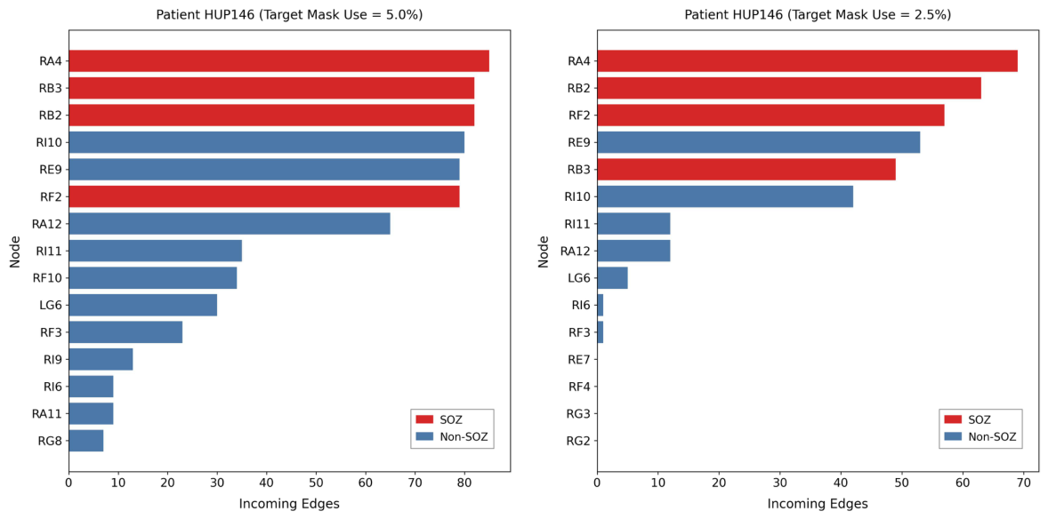
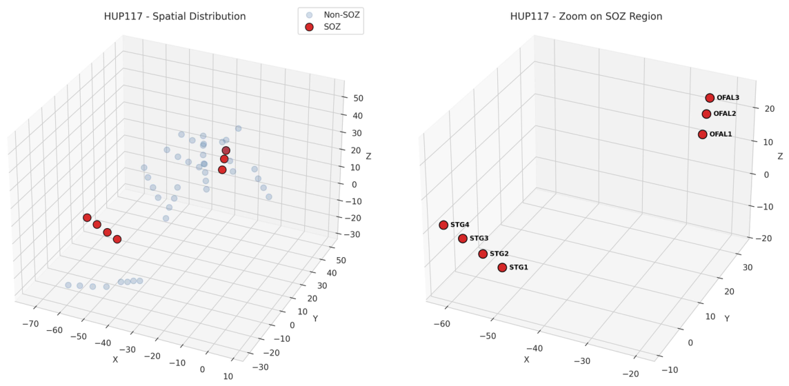
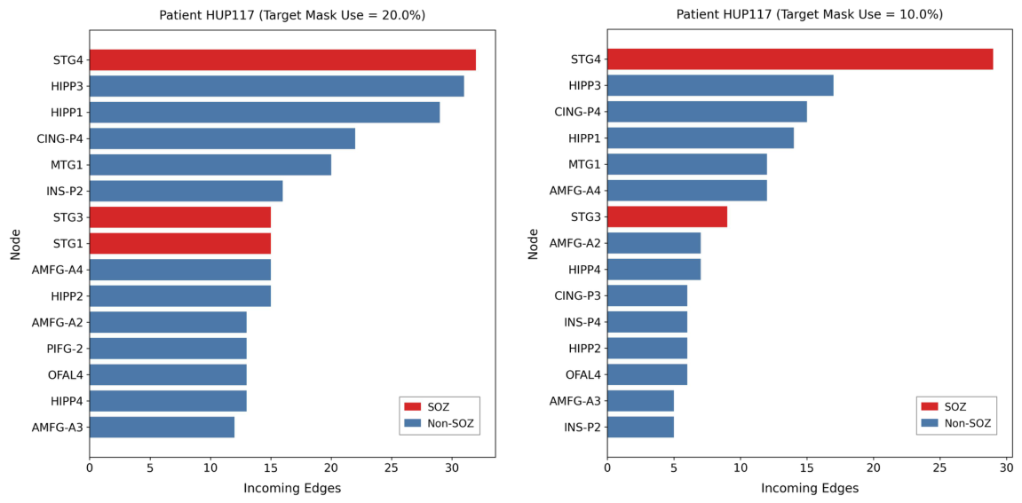
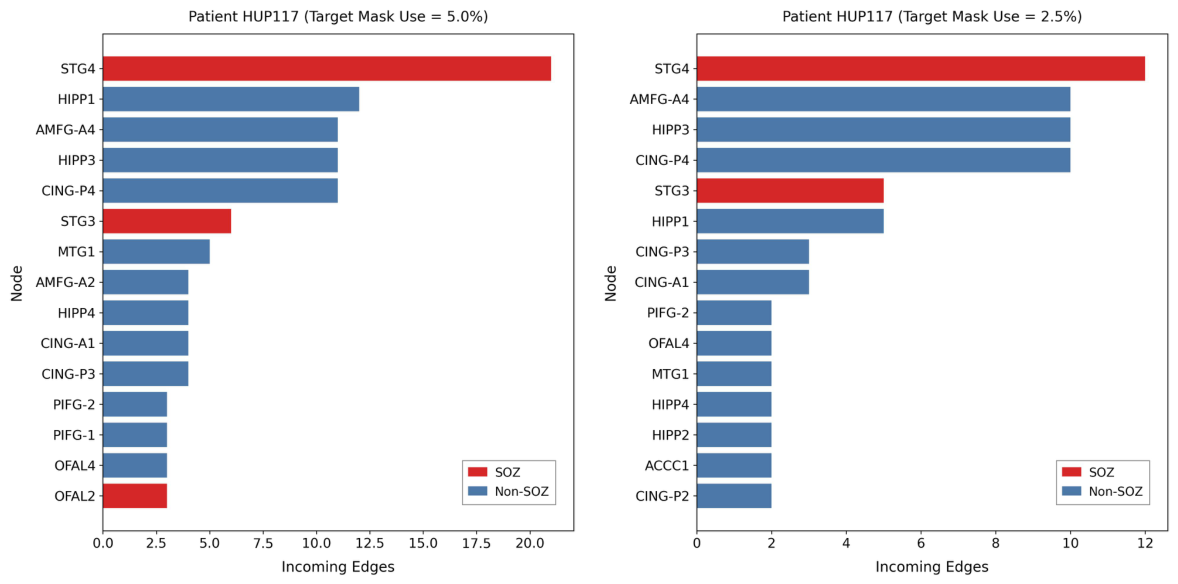
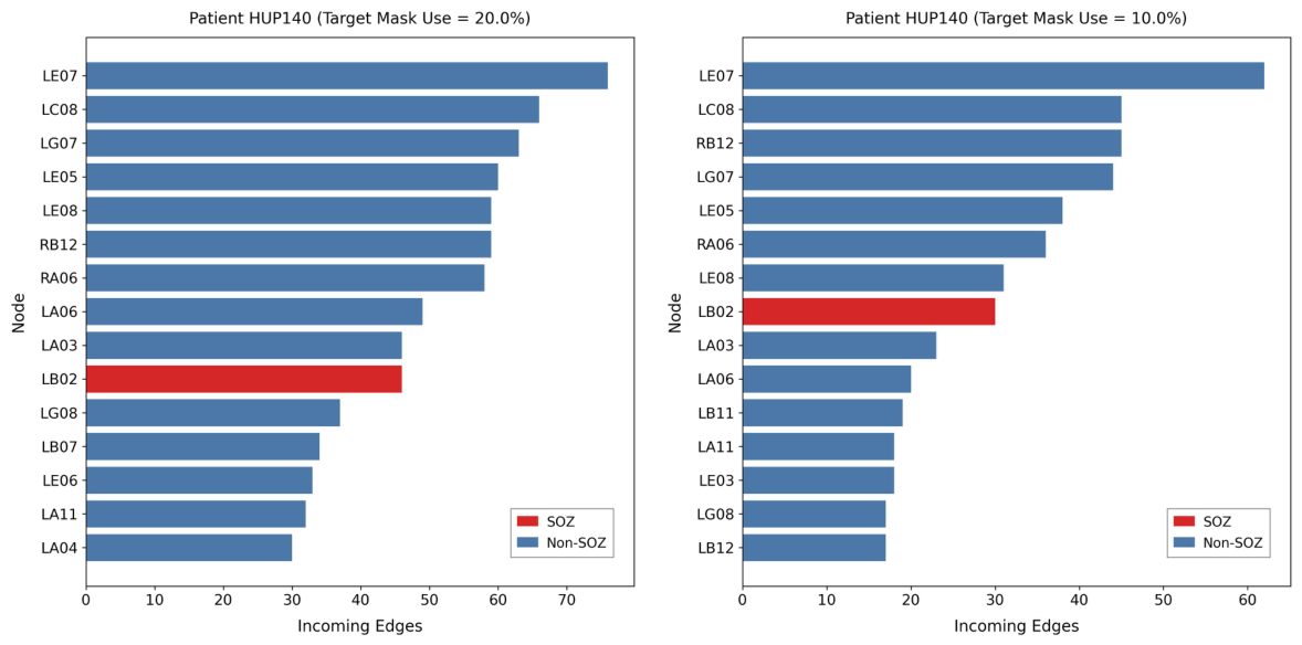
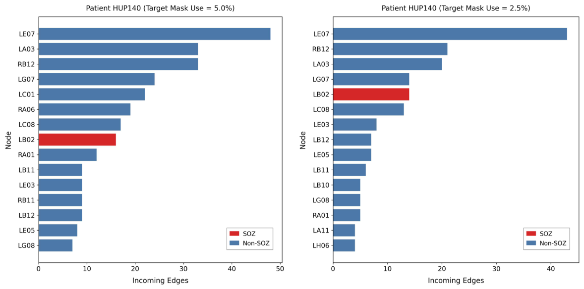
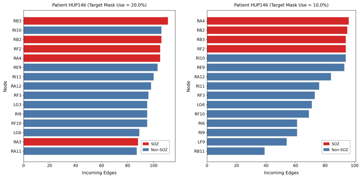
To analyze in greater detail how the relevance distribution evolves as the mask use is reduced, three representative cases were selected: HUP117, HUP140, and HUP146. These three examples illustrate different behaviors of the model. HUP117, shown in Figure 1 and Figure 2, represents an intermediate case, where the SOZ nodes appear overrepresented, although not particularly markedly. HUP140, shown in Figure 3 and Figure 4, corresponds to a more difficult case, in which the weight of the SOZ nodes is closer to their actual weight in the graph. Finally, HUP146, shown in Figure 5 and Figure 6, represents one of the most favorable cases. In this case, the concentration on SOZ nodes is clearly greater than their actual weight in the graph, and furthermore, this overrepresentation increases as $\gamma$ decreases.

In these examples, the aim is not only to observe whether SOZ nodes receive more incoming edges than non-SOZ nodes, but also to analyze how this distribution changes as the masking mechanism becomes more restrictive. Specifically, comparing different values of $\gamma$ allows us to examine whether reducing the number of active connections causes the model to focus on a smaller set of clinically significant nodes. In this way, these visualizations complement the aggregated results presented earlier and offer a more detailed view of the behavior of the explainability mechanism.

For these figures, the length of the bars indicates the number of incoming edges associated with each node, while the color is used solely to distinguish whether the node is labeled as SOZ or non-SOZ. Thus, the figures show how the incoming connections retained by the mask are distributed among the different nodes for each patient. These visualizations provide a detailed analysis at the patient level and are complemented by the quantitative results in Table 5 and Table 7, which summarize the cumulative percentage of incoming edges for SOZ and non-SOZ nodes.

In HUP117, as can be seen in Figure 1 and Figure 2, the model exhibits intermediate explanatory performance. SOZ nodes maintain a significant presence within the distribution of incoming edges, but this advantage is not as pronounced as in other patients. As the mask becomes more restrictive, the relevance tends to concentrate on a smaller set of nodes. However, non-SOZ nodes continue to appear with significant weight. Therefore, this case reflects a favorable trend toward concentration on clinically relevant nodes, although less clearly than in the more evident examples.

HUP140 represents a more challenging case from the perspective of explainability, as shown in Figure 3 and Figure 4. In this patient, the weights of the SOZ nodes remain relatively close to their actual weights within the graph, and the observed overrepresentation is limited. Although reducing the mask size also causes relevance to be distributed among fewer nodes, the relative advantage of the SOZ nodes remains moderate. Therefore, this example is useful for demonstrating that the model’s general tendency does not manifest with the same intensity in all patients and that there are cases where the correspondence between inferred relevance and clinical annotation is weaker.

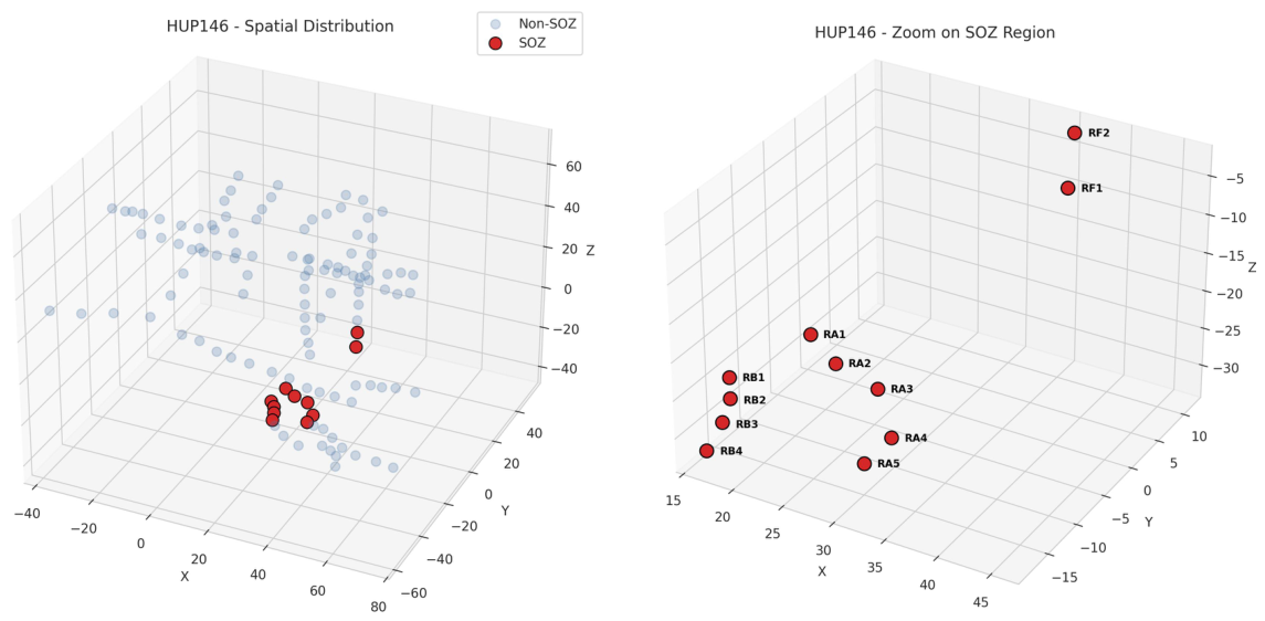
In HUP146, one of the clearest patterns is observed, as can be seen in Figure 5 and Figure 6. In this patient, the SOZ nodes concentrate a proportion of incoming edges far greater than what would correspond to their actual weight in the graph. Furthermore, as $\gamma$ decreases, this overrepresentation increases, so that the relative relevance of the SOZ nodes becomes increasingly evident. This makes HUP146 a particularly illustrative example of the behavior sought in the model’s explainability mechanism, since the restriction on connections not only simplifies the structure used but also reinforces the concentration of relevance in the clinically most significant nodes.

4.6. Perturbation Analysis

To complement the analysis based on correspondence with SOZ nodes, a perturbation analysis was performed on the graph nodes. The objective of this analysis is to evaluate whether the nodes identified as most relevant by the mask have a functional impact on the model’s prediction. The relevance of each node was defined based on the number of incoming edges received in the learned mask. Five strategies were compared: perturbing the most relevant nodes, random nodes, low-relevance nodes, SOZ nodes and non-SOZ nodes. For this analysis, the perturbation was defined as a controlled removal of the information associated with specific nodes. Therefore, the values of the selected nodes were replaced with zero throughout the entire time series in the test set, and the drop in performance relative to the unperturbed model was measured. This strategy allows the graph structure and the model’s propagation flow to remain constant, modifying only the input information available at the analyzed nodes. This type of node feature occlusion is used in GNNs because it allows the contribution of nodes to be studied without altering the graph topology [23,37].

This type of perturbation was chosen because it was more suitable for the analysis objective than other alternatives. In this work, the model input includes the line length feature calculated per window and channel. Therefore, using Gaussian noise would be less straightforward to interpret and would introduce an additional source of variability depending on the noise distribution used. Furthermore, replacing the values with the node’s temporal mean could preserve some of the channel’s information, so it would not represent such a direct elimination of its contribution. In addition, since the replacement with zero is applied consistently throughout the entire time sequence of the selected node, the perturbation does not introduce point-specific fluctuations or local discontinuities within the time representation processed by the GRU. Its effect should be interpreted as the suppression of information from that channel during the sequence, not as the generation of an artificial time dynamic.

The results in

Table 8. Analysis of node relevance perturbation. The table shows the absolute drop in performance, measured relative to the unperturbed model, after perturbing different groups of nodes in the test set. The top relevance nodes are selected based on the number of incoming edges in the learned mask. The random nodes are averaged across multiple random runs. In the case of SOZ nodes, all nodes of this type are affected, whereas in the case of non-SOZ nodes, the number of affected nodes is equal to the number of SOZ nodes.

Perturbation	k	Accuracy Drop	F1 Drop	ROC-AUC Drop
Top relevance nodes	5%	0.093 ± 0.118	0.543 ± 0.354	0.078 ± 0.144
Top relevance nodes	10%	0.098 ± 0.123	0.600 ± 0.340	0.085 ± 0.144
Top relevance nodes	20%	0.103 ± 0.123	0.622 ± 0.334	0.087 ± 0.149
Random nodes	5%	0.013 ± 0.056	0.025 ± 0.103	0.003 ± 0.018
Random nodes	10%	0.028 ± 0.100	0.061 ± 0.161	0.006 ± 0.033
Random nodes	20%	0.048 ± 0.138	0.124 ± 0.221	0.012 ± 0.052
Low relevance nodes	5%	0.002 ± 0.013	0.006 ± 0.031	0.001 ± 0.006
Low relevance nodes	10%	0.001 ± 0.029	0.014 ± 0.070	0.002 ± 0.007
Low relevance nodes	20%	0.009 ± 0.069	0.029 ± 0.119	0.003 ± 0.010
SOZ nodes	all SOZ	0.050 ± 0.105	0.267 ± 0.355	0.046 ± 0.082
Non-SOZ nodes	SOZ count	0.050 ± 0.146	0.068 ± 0.164	0.006 ± 0.029

show that perturbing the most relevant nodes results in a significantly greater degradation than perturbing random nodes or low-relevance nodes. In particular, when perturbing 5%, 10%, and 20% of the most relevant nodes, the average drop in F1 is 0.543, 0.600, and 0.622, respectively. These drops are much larger than those observed in accuracy, which is consistent with the unbalanced nature of the problem. While accuracy is strongly influenced by the interictal class, F1 more directly reflects the deterioration in the detection of the ictal class. Therefore, the strong reduction in F1 indicates that perturbing the most relevant nodes particularly affects the model’s ability to identify ictal segments. In contrast, the perturbation of random nodes produces F1 drops of 0.025, 0.061, and 0.124 for the same percentages, while the perturbation of low-relevance nodes produces even smaller drops. This indicates that the nodes selected by the mask play a significant role in the model’s decision-making.

The perturbation of SOZ nodes also results in a greater degradation than the perturbation of an equivalent number of non-SOZ nodes, particularly in F1 and ROC-AUC. However, the most significant drop is observed when perturbing the nodes with the highest relevance according to the mask. This suggests that the mask captures information that is functionally relevant to the model and that this information is related, though not exclusively, to nodes annotated as SOZ. Therefore, the perturbation analysis reinforces the interpretation of the mask as an internal explanatory mechanism, complementing the analysis based on correspondence with SOZ nodes.

4.7. Spatial Analysis of SOZ Nodes

In addition to analyzing the learned mask, the spatial organization of the SOZ nodes was also studied based on the three-dimensional location of the electrodes. To this end, two complementary measures were used. First, the average distance between each SOZ node and its nearest node of the same class was calculated and compared with the average distance between each non-SOZ node and the nearest SOZ node. Second, the proportion of SOZ nodes among the three closest spatial neighbors of each electrode was estimated. Furthermore, this information was summarized using ROC-AUC. This analysis allows us to assess the extent to which the spatial structure of the electrodes contains useful information for distinguishing between SOZ nodes and non-SOZ nodes.

The results show a very consistent spatial correlation. On average, the distance between an SOZ node and its nearest neighbor of the same class was 5.48, while the distance between a non-SOZ node and the nearest SOZ node was 46.28. Complementarily, the average percentage of SOZ neighbors among the three nearest neighbors was 74.9% for the former, compared to 3.0% for non-SOZ nodes, and the average ROC-AUC reached 0.979. Taken together, these values indicate that these nodes are not randomly distributed but tend to appear spatially clustered. Non-SOZ nodes, on the other hand, are typically found farther away from these clusters. This is relevant because it suggests that, once one of these nodes is identified, the surrounding area is much more likely to contain other nodes of the same class than non-SOZ nodes. From this perspective, the model’s detection of relevant nodes not only provides explainability but could also help to narrow the search for other regions of clinical interest in an informed manner.

The 3D visualizations of HUP117, HUP140, and HUP146, shown in Figure 7, Figure 8 and Figure 9, reveal this spatial pattern. In all three cases, it can be seen that the SOZ nodes appear clustered in specific regions of space and are not randomly scattered throughout the set of electrodes. Furthermore, several of the nodes that accumulated a greater number of incoming edges in the previous figures are found precisely within these clusters or in their immediate surroundings. This reinforces the idea that the model’s behavior is not only consistent with the clinical annotation of the SOZs but also with their spatial organization. Thus, an additional interpretation of the learned explanatory mechanism is provided.

To complement this spatial analysis, the adjacency inferred by ESEGCRN was compared with the distance between nodes. Using the three-dimensional coordinates of each electrode $p_i=(x_i,y_i,z_i)$, a Euclidean distance matrix was constructed, defined as

$$D_{ij}=\parallel p_i-p_j\parallel ,$$

(13)

where $D_{ij}$ represents the physical distance between nodes i and j. The analysis was performed at the patient level, excluding self-connections and considering only nodes with available 3D coordinates. If the learned adjacency were dominated by proximity, a negative correlation would be expected between the adjacency values and D, since the strongest connections should occur between physically closer electrodes.

The results showed a Spearman correlation coefficient of virtually zero between the learned adjacency and the distance between electrodes ($0.026\pm 0.045$). This indicates that the connections learned by the model do not systematically increase or decrease as a function of the distance between nodes. Furthermore, the average distance of active connections was similar to that of inactive connections, with values of $65.3\pm 11.2$ and $61.6\pm 11.5$, respectively. Furthermore, no concentration of active connections was observed among the closest physical neighbors, as the proportion of active connections among the 3, 5, and 10 closest neighbors was lower than the overall percentage of active connections.

4.8. Ablation Study

To analyze the impact of the modifications introduced by ESEGCRN in greater detail, an ablation study was conducted with $\gamma =2.5\%$. This analysis compares four variants. The first corresponds to SEGCRN, used as the baseline. The second incorporates the exact binary mask via STE, keeping the rest of the formulation as close as possible to SEGCRN. The third also adds the mask shared between layers, but still retains the previous loss function. Finally, ESEGCRN incorporates all the proposed changes, namely the exact binary mask, the shared mask between layers and the modified loss function. In this way, it is possible to study the progressive effect of each modification on predictive performance, mask sparsity, the concentration of relevance in SOZ nodes and the stability of the explainability.

Table 9. Ablation study for different configurations with $\gamma =2.5\%$. EBM refers to exact binary mask and SM to shared mask. The best result for each metric is shown in bold.

Variant	Mask Use	Accuracy	Precision	Recall	F1	Specificity	NPV	ROC-AUC
SEGCRN	47.4% ± 0.2%	93.5% ± 0.8%	85.7% ± 1.7%	84.4% ± 2.0%	83.3% ± 2.1%	95.3% ± 0.8%	96.7% ± 0.4%	94.6% ± 0.2%
EBM	29.5% ± 1.8%	94.1% ± 0.6%	87.7% ± 1.6%	85.0% ± 1.3%	84.9% ± 1.6%	96.0% ± 0.8%	96.7% ± 0.2%	94.2% ± 0.8%
EBM + SM	29.5% ± 1.8%	94.2% ± 0.8%	88.2% ± 2.2%	83.2% ± 1.8%	84.3% ± 2.0%	96.5% ± 0.9%	96.3% ± 0.4%	94.3% ± 0.6%
ESEGCRN	2.7% ± 0.0%	93.1% ± 1.6%	87.8% ± 2.2%	79.7% ± 3.0%	81.4% ± 2.8%	95.9% ± 2.0%	95.7% ± 0.6%	94.1% ± 0.8%

shows the prediction metrics obtained for each variant. The intermediate variants maintain performance very similar to that of SEGCRN and even achieve the best values on some metrics. In contrast, ESEGCRN reduces mask usage to 2.7%, while maintaining competitive performance. This difference highlights the main trade-off introduced by the full formulation. ESEGCRN applies a much stronger restriction on information propagation, resulting in a moderate loss of predictive performance, but with a much sparser and easier to analyze relational structure.

Table 10. Ablation study of mask usage and SOZ incoming edge concentration for $\gamma =2.5\%$. EBM refers to an exact binary mask, and SM refers to a shared mask.

Variant	Mask Use	SOZ Nodes	SOZ IE	Non-SOZ IE	SOZ IE(%)	Non-SOZ IE(%)
SEGCRN	47.4% ± 0.2%	9.6% ± 0.0%	57.85 ± 0.16	61.11 ± 0.21	9.1% ± 0.0%	90.9% ± 0.0%
EBM	29.5% ± 1.8%	9.6% ± 0.0%	51.53 ± 0.87	29.33 ± 2.92	15.7% ± 1.1%	84.3% ± 1.1%
EBM + SM	29.5% ± 1.8%	9.6% ± 0.0%	56.10 ± 1.26	27.93 ± 2.75	17.6% ± 1.1%	82.4% ± 1.1%
ESEGCRN	2.7% ± 0.0%	9.6% ± 0.0%	10.00 ± 0.71	2.64 ± 0.05	28.6% ± 1.8%	71.4% ± 1.8%

shows the effect of these modifications on the concentration of incoming edges at SOZ nodes. In SEGCRN, the percentage of SOZ incoming edges is close to the percentage of SOZ nodes, indicating a limited concentration of relevance in the clinically annotated regions. The introduction of the exact binary mask increases this percentage, and the shared mask increases it slightly further. Finally, ESEGCRN achieves the highest concentration of incoming edges at SOZ nodes, at 28.6%. This suggests that the complete formulation not only restricts the propagation of information but also promotes a selection more consistent with the SOZ nodes.

In addition to predictive performance and concentration on SOZ nodes, mask stability was analyzed. This analysis was conducted from two complementary perspectives. First, the evolution of overall mask usage during training was studied to determine when it stabilizes. Second, stability across masks was analyzed, which is particularly relevant for comparing variants with independent masks versus variants with a shared mask.

Table 11. Ablation study of mask stability for $\gamma =2.5\%$. Relevance Change indicates the average layer-wise variability of node relevance. Jaccard Index indicates the average similarity between layer masks. Stable Epoch indicates the approximate epoch at which the use of the global mask stabilizes. EBM refers to the exact binary mask and SM to the shared mask.

Variant	Stable Epoch	Relevance Change	Jaccard Index
SEGCRN	98.2	1.30	0.370
EBM	120.0	9.02	0.330
EBM + SM	120.7	0.00	1.000
ESEGCRN	28.0	0.00	1.000

summarizes these results.

Regarding mask stability during training, the stable epoch was defined as the first epoch after which the validation mask use remains within an absolute tolerance of 0.005 of its final value until the end of training. Since the mask use is expressed in the range $[0,1]$, this tolerance is equivalent to 0.5%. Under this criterion, ESEGCRN achieves this stability around epoch 28, while the remaining variants require a considerably larger number of epochs. This indicates that ESEGCRN stabilizes the generated mask sooner. However, this analysis refers to the overall use of connections during training, so it should not be interpreted on its own as a complete measure of the stability of each node’s relevance. For this reason, it is complemented by an analysis of stability between masks at the layer level.

In this analysis, the relevance change indicates the average variability in the relevance of nodes across layers. It is calculated based on the standard deviation of the number of incoming edges received by each node in the different layers. Therefore, higher values indicate that the importance assigned to nodes varies more across layers, while a value of 0 indicates that relevance remains constant across them. In addition, the Jaccard index measures the similarity between the active connections in the masks of different layers. Values close to 1 indicate that the layers use virtually the same connection structure, while lower values indicate that the masks differ more significantly across layers.

In the variants with independent masks per layer, SEGCRN and EBM in Table 11, the relevance assigned to nodes may vary across layers. This is reflected in their relevance change values, which are greater than 0, and in their Jaccard index values, which are well below 1. Furthermore, the mask of a later layer is applied to representations that have already been transformed and propagated through previous layers. Therefore, the interpretation of that mask does not refer exactly to the same information as in the first layer, which makes it difficult to obtain a single interpretation of the relational structure used by the model. In contrast, variants with a shared mask exhibit a relevance change of 0 and a Jaccard index of 1, since the same relational structure is used across all layers. In particular, ESEGCRN combines this structural stability with earlier stabilization of the mask’s global usage during training, which reinforces the interpretation of the mask as a more stable and directly analyzable mechanism.

Overall, the ablation study shows that the modifications introduced in ESEGCRN should not be interpreted as changes aimed at maximizing predictive performance. Intermediate variants achieve highly competitive results, but ESEGCRN provides the most restrictive, stable, and consistent formulation from the perspective of explainability. Therefore, the main contribution of the proposal lies in the balance between maintaining competitive predictive performance and obtaining a sparser, more stable mask that is better aligned with the SOZ nodes.

5. Discussion

The results obtained should be interpreted in light of the two data splitting strategies used in this study. On the one hand, under the sample-level split used in previous works, ESEGCRN demonstrates highly competitive performance and achieves the best results among the compared methods under this evaluation setting. On the other hand, under the temporal-block strategy, the model maintains solid performance in a more conservative scenario. In this scenario, the risk that temporal proximity between samples leads to overly optimistic estimates is reduced. This dual evaluation allows for a clearer distinction between comparability with previous work and the methodological analysis of the model.

The difference between these two scenarios allows us to partially quantify the impact of potential bias associated with the use of overlapping windows. In this study, each sample covers a 7 s sequence and is generated with a 1 s stride. Therefore, two consecutive samples share 6 of the 7 s of signal, which equates to a maximum overlap of 85.7%. Although not all consecutive pairs end up in the same partition, since only 70% is used for training, there remains a high risk of overlap. Furthermore, samples separated by several seconds may still share part of the original time interval. Consequently, a random sample-level split may place very similar or partially overlapping sequences in the training, validation, and test sets, leading to an optimistic estimate of performance. With the sample-level split, ESEGCRN achieves 98.3% accuracy and 95.9% F1 score when compared to previous work. In contrast, under the temporal-block strategy, the best overall performance obtained is 94.4% accuracy and 84.5% F1. This reduction confirms that sample-level partitioning can produce a more favorable performance estimate when there are temporally close or partially overlapping windows across different partitions. For this reason, the sample-level split is retained solely for the purpose of comparing results with other models that use this strategy. In contrast, the temporal-block evaluation is used for detailed analysis of performance and explainability.

In this context, one of the most significant findings of this study is that progressively restricting the mask does not cause a sharp decline in the model’s performance. Although the best overall predictive setting corresponds to $\gamma =20.0\%$, the more restrictive settings still maintain solid metrics. At the same time, they facilitate a clearer interpretation of the explanatory mechanism. In particular, by reducing mask use, the model tends to concentrate an increasing proportion of incoming edges on SOZ nodes. This suggests that, by limiting the number of active connections, the architecture uses the available spatial information more selectively and tends to focus its decision-making on regions more consistent with clinical information.

A patient-by-patient analysis reinforces this idea. In most cases, SOZ nodes concentrate a proportion of incoming edges greater than their actual weight within the set of nodes, which provides confidence in the internal consistency of the explainability mechanism. Furthermore, the examples analyzed in detail show a consistent trend. As mask usage decreases, relevance concentrates on a smaller subset of nodes, and SOZ nodes become more relevant. However, this behavior is not entirely uniform across all patients. There are cases where the concentration on SOZ nodes is less pronounced. This indicates that, although the model’s overall trend is favorable, the relationship between explainability and clinical annotation can still be improved.

The worst-case scenario in this analysis corresponds to HUP177. For this patient, the model maintains relatively high accuracy and specificity, but achieves low recall and F1 scores, indicating that the main challenge lies in detecting the ictal class. Furthermore, it is the only case in which the mask does not concentrate incoming edges on SOZ nodes. A review of the data shows that HUP177 has one of the largest graphs, a relatively low proportion of SOZ nodes, and a level of ictal activity below the average of the other patients. These factors may make it difficult to learn a discriminative representation of the ictal class and to concentrate relevance in the SOZ nodes. However, with the available information, it is not possible to attribute this behavior to a specific clinical cause, such as a particular seizure morphology or a specific implantation configuration. Therefore, this patient should be interpreted as a borderline case.

This behavior also suggests that, in particularly difficult cases, it may be necessary to adjust $\gamma$ on a patient-specific basis. In HUP177, less restrictive mask settings show better predictive performance than $\gamma =2.5\%$. Specifically, with $\gamma =20.0\%$, the model achieves 91.0% accuracy, 61.1% recall, and 66.7% F1 score, whereas with $\gamma =2.5\%$ these values drop to 84.4%, 33.3%, and 38.7%, respectively. This difference suggests that, in this patient, excessive masking particularly limits the detection of the ictal class, as reflected by the drop in recall and F1. This observation is consistent with the general trend shown in Table 4, where higher values of $\gamma$ maintain slightly better predictive metrics.

A relevant aspect of this work is the variation in graph size across patients. This disparity is addressed through a patient-specific approach, such that each model is trained and evaluated using the set of nodes corresponding to a single patient. Therefore, the architecture does not require all subjects to have the same number of channels. Furthermore, the mask usage is calculated as a proportion of the total number of possible connections, allowing for a comparison of the sparsity between graphs of different sizes. The results do not show a systematic degradation in performance or explainability when the number of nodes increases. For example, some patients with large graphs maintain high performance and a clear concentration of incoming edges at SOZ nodes. This indicates that the model’s behavior does not depend on the number of nodes, but rather on the quality of the available signals, the distribution of SOZ nodes and the variability specific to each patient.

Another noteworthy aspect is the spatial organization observed in SOZ nodes. The results show that these nodes tend to cluster spatially and that, once one is identified, the probability of finding other SOZ nodes in its immediate vicinity increases. This property is interesting because it suggests that the model’s explainability could provide useful information beyond simply justifying a binary prediction. In particular, the identification of particularly relevant nodes could help narrow down regions of interest on which to initiate a more detailed analysis. Although this work does not propose a clinical localization tool, it does provide indications that the explainability mechanism could serve as a guide for subsequent analyses.

Nevertheless, these results should be interpreted with caution. The study presented here should be understood as an experimental validation on a specific dataset under controlled conditions. The fact that ESEGCRN achieves very high performance and demonstrates consistent explanatory behavior provides strong evidence of the approach’s potential. However, this does not in itself constitute clinical validation. In a medical problem such as this, any potential real-world application requires further evaluation using other datasets, specific clinical studies, and a more in-depth analysis of the model’s robustness and generalizability.

The False Activation Rate (FAR) was also analyzed to contextualize specificity in a long-term monitoring scenario. FAR was calculated over the evaluated interictal period, as it measures the number of false activations occurring in the absence of a seizure. Since several consecutive windows may correspond to a single activation, the main analysis was performed at the event level, grouping consecutive or closely spaced false positives. By grouping consecutive false positives, ESEGCRN yields a FAR of 23.5 false alarm events/hour, and by allowing a 10 s tolerance between activations, this is reduced to 19.3 false alarm events/hour. Furthermore, by requiring 3 consecutive positive windows, the FAR is reduced to 11.7 false alarm events/hour, while applying an alarm suppression period of 60 s yields a FAR of 14.6 false alarm events/hour. As an additional exploratory analysis, combining a threshold of 0.9 with an alarm suppression period of 60 s reduces the FAR to 5.6 false alarm events/hour. However, this result involves modifying the decision threshold and should be interpreted as a sensitivity analysis, not as the primary configuration evaluated in the study.

These results show that, although the model achieves high specificity in seizure detection, its direct use as an alarm system would still produce a high number of false activations unless specific calibration is incorporated. Therefore, ESEGCRN should be interpreted in this study as a seizure detection model with built-in explainability, not as a standalone clinical alarm system. To convert these predictions into appropriate alarm events, it would be necessary to explore strategies that take into account the temporal continuity of the signal. For example, it would be possible to consider temporal smoothing, event merging to group consecutive or very close activations, and refractory periods to avoid generating multiple alarms associated with the same episode [38,39]. Furthermore, the decision threshold should be calibrated considering not only classification performance but also the acceptable number of false alarms per hour in a continuous monitoring scenario. In this regard, adaptive strategies could be particularly relevant, as the balance between sensitivity and false alarms can vary across patients and recording conditions [40]. Therefore, as part of future work, the model should be evaluated alongside such post-processing mechanisms, with the aim of analyzing its feasibility in scenarios closer to clinical monitoring.

Another significant limitation relates to generalization across patients. In this study, the model is formulated on a patient-specific basis, since each subject has a different number of channels, a different spatial layout, and a unique relational structure. Therefore, there is no direct correspondence between the nodes of different patients. This means that a cross-patient evaluation is not straightforward with the current approach, since training the model on some patients and applying it to others would require first defining a common representation of the nodes. Future work could address this problem through common node representations, adaptation strategies across patients, or by combining multi-patient learning with subsequent subject-specific fine-tuning.

One possible approach would be to project the nodes onto a common space and associate them with regions [41]. Under this approach, the graph nodes would not be specific to individual patients, but rather represent regions that are comparable across patients. Another possibility would be to use graph alignment to establish correspondences between graphs from different patients, taking into account both the position of the electrodes and the similarity of their patterns [42]. Hybrid approaches could also be explored, in which a shared representation is learned from multiple patients and subsequently fine-tuned on a patient-specific basis to adapt the model to each subject’s unique implantation and dynamics. These approaches would allow progress toward models with greater generalization capacity, although they would require an explicit reformulation of the problem and specific validation.

Overall, the results of this work show that ESEGCRN achieves very high performance while incorporating an analyzable internal explainability mechanism. This reinforces the value of continuing to develop this type of approach for graph-based seizure analysis problems. In particular, to study in greater detail cases where the focus on SOZ nodes is less clear and to analyze the extent to which such mechanisms can contribute to tasks of greater clinical interest.

6. Conclusions

This paper presents ESEGCRN, an improved version of SEGCRN that is better suited for the problem of seizure detection in iEEG in a patient-specific setting. The proposed approach reformulates the masking mechanism of the original model with the aim of making its behavior more consistent and promoting a more stable interpretation of node relevance. The evaluation shows that ESEGCRN exhibits high predictive power for this problem and achieves highly competitive performance compared to the models included in the comparison. This indicates that the proposed reformulation not only allows the architecture to be adapted to a new domain but also maintains robust classification performance. In this regard, the results obtained underscore the value of this type of approach for the analysis of multichannel iEEG signals.

Furthermore, a detailed analysis of the results showed that, as the restriction on the use of connections increases, the model tends to progressively concentrate incoming edges on SOZ nodes. This reinforces the internal consistency of the explanatory mechanism and suggests that the relevance inferred by the model is, in many cases, related to clinically significant information. Although the best configuration from a predictive standpoint corresponds to the least restrictive case analyzed, the more restrictive configurations still exhibit robust performance and allow for a clearer observation of this explanatory trend. Therefore, the proposal is not only useful from a predictive standpoint but also for interpreting the model’s internal behavior. In addition, spatial analysis showed that SOZ nodes tend to cluster together. This suggests that the model’s explainability could provide useful information beyond binary classification by highlighting the most relevant nodes.

Overall, this study shows that a spatio-temporal model with an internal explainability mechanism can be adapted to the problem of seizure detection in iEEG while maintaining competitive performance and providing useful information about channel relevance. However, the results must be interpreted with several limitations in mind. First, the evaluation was conducted on a single dataset and in a patient-specific scenario, so the model’s generalization ability needs to be further explored. Second, since the model was designed for a patient-specific scenario, it cannot be directly applied to cross-patient scenarios. Furthermore, the FAR analysis shows that ESEGCRN should not be interpreted as a standalone clinical alarm system without additional calibration, temporal post-processing, and validation on long-term continuous recordings. Therefore, these results should be interpreted with caution, bearing in mind that the work presented constitutes an experimental validation on a specific dataset and not a clinical validation of the model.

Therefore, as future work, it will be of interest to evaluate the performance of ESEGCRN on other datasets and analyze its behavior in scenarios with greater variability. It will also be necessary to study cross-patient generalization strategies, for example through common representations, graph alignment, or pre-training schemes followed by patient-specific fine-tuning. Finally, it will be necessary to develop post-processing strategies that reduce the number of false alarm events and to validate the model on long-term continuous recordings in scenarios more closely resembling real-world clinical monitoring.