Phase-Space Structure and Traveling-Wave Solutions of a (3 + 1)-Dimensional Extended Kadomtsev–Petviashvili Equation

Abstract

This study investigates the ($3+1$)-dimensional extended Kadomtsev–Petviashvili equation via traveling-wave phase-space geometry. The equation is reduced to a planar Hamiltonian system with cubic nonlinearity, whose conserved energy partitions the phase space into periodic orbits, separatrices, and unbounded trajectories. Closed-form profiles for the gradient variable $\phi =U_{\xi }$ are obtained through separation of variables; the corresponding field U is recovered by quadrature and must satisfy a zero-mean condition for periodic reconstruction. In particular, for $h_1>0$, the reconstructed field exhibits kink/antikink-type rather than localized-pulse behavior. Under weak periodic forcing, an explicit Melnikov amplitude factor is derived. Its exponential decay with the forcing frequency implies that the leading-order separatrix splitting distance $\mu A\left(\omega \right)$ becomes exponentially small at high frequency, while the simple-zero condition still predicts transverse intersections of stable and unstable manifolds and the onset of horseshoe chaos. Applying the complete discriminant method yields eight distinct solution families—hyperbolic, trigonometric, rational, and Jacobi elliptic—each associated with a unique orbital topology. These results enrich both the dynamical theory and the exact solution framework of higher-dimensional nonlinear evolution equations.

1. Introduction

Nonlinear partial differential equations (NPDEs) model multidimensional wave phenomena in fluids, plasmas, and nonlinear optical media [1,2]. In such systems, the interplay of weak dispersion and weak nonlinearity generates solitary waves [3,4,5], lumps [6,7], breathers [8,9], and their interactions [10,11]. The Kadomtsev–Petviashvili (KP) family and its higher-dimensional extensions describe quasi-two-dimensional and fully three-dimensional wave dynamics in weakly dispersive media [12,13].

The traveling-wave ansatz reduces NPDEs to lower-dimensional ordinary differential equations (ODEs) [14,15], enabling phase-space analysis, bifurcation studies, and chaos diagnostics [16]. In the resulting planar dynamical system, homoclinic orbits correspond to solitary waves, and closed orbits to periodic waves. This orbit–wave correspondence allows parameter-dependent classification via equilibrium types and bifurcations.

The KP equation, originally a transverse extension of the KdV equation, remains central to multidimensional weakly dispersive wave modeling. Several extensions incorporate higher-order dispersion and mixed derivatives [17]. The following extended KP equation is considered:

$$\begin{array}{c}\hfill u_{xxxy}+3{\left(u_x{u}_y\right)}_x+\alpha u_{xxxz}+3\alpha {\left(u_x{u}_z\right)}_x+{ϵ}_1{u}_{xt}+{ϵ}_2{u}_{yt}+{ϵ}_3{u}_{zt}+{\omega }_1{u}_{xz}+{\omega }_2{u}_{yz}+{\omega }_3{u}_{zz}=0,\end{array}$$

(1)

where $\alpha$, ${ϵ}_i$ and ${\omega }_i$ are real parameters. Appropriate parameter choices recover known integrable models (e.g., Jimbo–Miwa [18] and KP types [19]), making Equation (1) a unified testbed for high-dimensional nonlinear waves.

Following the full-parameter setting of the ($3+1$)-D KP framework, the specific parametrization is adopted:

$$u_{xxxy}+3{\left(u_x{u}_y\right)}_x-u_{xxxz}-3{\left(u_x{u}_z\right)}_x+u_{xt}+u_{yt}-u_{zt}+u_{xz}+u_{yz}+u_{zz}=0,$$

(2)

which yields a complete ($3+1$)D KP-type configuration balancing dispersive, convective, and mixed-derivative effects.

This work builds on previous bilinear–neural network studies [20], which produced block, soliton, and periodic solutions to Equation (2). Although those results enriched the explicit solution repertoire, they did not provide a global description of traveling-wave dynamics via phase portraits, bifurcation scenarios, or chaotic mechanisms. The present paper adds global dynamic trajectory classification, explicit Melnikov chaos analysis, and eight complete topological corresponding analytical solution systems to fill the previous research gap.

Equation (1) generalizes the classical KP form introduced by Kadomtsev and Petviashvili (1970) to describe transversely modulated KdV waves [21]:

$${(u_t+6u{u}_x+u_{xxx})}_x+3{\sigma }^2{u}_{yy}=0,$$

(3)

where $u=u(x,y,t)$ and subscripts denote partial derivatives; in particular, $u_t=\mathsf{\partial }u/\mathsf{\partial }t$, $u_x=\mathsf{\partial }u/\mathsf{\partial }x$, $u_{xxx}={\mathsf{\partial }}^{3}u/\mathsf{\partial }{x}^3$, and $u_{yy}={\mathsf{\partial }}^{2}u/\mathsf{\partial }{y}^2$.

Most existing studies on KP-type equations have relied on bilinearization [22,23,24] or ansatz methods [25] to construct explicit exact solutions, yielding multi-solitons, lumps, and interaction patterns [26,27]. Recent work on ($3+1$)D generalized KP models has advanced this direction via three main avenues: (i) constructing particular solutions using complex separated variables and variational principles [28,29]; (ii) exploring nonlocal extensions via generalized bilinear derivatives [30,31]; and (iii) incorporating extra time or space derivatives to capture rogue waves and breaking phenomena [32,33,34]. Despite these advances alongside our recent bilinear–neural framework results, a systematic dynamical-system characterization of traveling waves for Equation (2), covering phase-space structure, trajectory topology, separatrix roles, orbit–solution correspondence, and Melnikov-theoretic chaos [35,36,37,38], remained absent. Addressing this gap motivates the present work.

The remainder of the paper is organized as follows. Section 2 reduces the traveling-wave ODE to a Hamiltonian system, classifies orbit topology via the first integral, and derives closed-form separatrices revealing kink-type reconstruction. Section 3 analyzes the periodically perturbed system, presents Melnikov criteria for separatrix splitting, and demonstrates chaos with sensitivity to initial conditions. Section 4 constructs closed-form exact solutions via discriminant classification. Section 5 displays representative wave profiles. Section 6 concludes and discusses extensions.

2. Traveling-Wave System, Hamiltonian Structure, and Orbit Topology

2.1. Reduced Planar Hamiltonian System

To analyze Equation (2), the traveling-wave ansatz is adopted as:

$$u(x,y,z,t)=U\left(\xi \right),\xi =kx+ly+mz-ct,$$

(4)

where U is real and $k,l,m$ are nonzero parameters determining the wave speed. This ansatz reduces Equation (2) to an ODE for U.

$$\left(k^{3}l-k^{3}m\right)U^{\left(4\right)}+\left(6k^{2}l-6k^{2}m\right)U^{\prime }{U}^{″}+\left(m^2+lm+km+mc-kc-lc\right)U^{″}=0.$$

(5)

Integrating Equation (5) once gives

$$\begin{array}{c}\hfill \left(k^{3}l-k^{3}m\right)U^{\left(3\right)}+\left(3k^{2}l-3k^{2}m\right){\left(U^{\prime }\right)}^2+\left(m^2+lm+km+mc-kc-lc\right)U^{\prime }+C_I=0,\end{array}$$

(6)

where $C_I$ is an integration constant. In the present work, we restrict our attention to the zero-integration-constant class $C_I=0$. This choice is compatible with the homoclinic/separatrix boundary conditions

$$U^{\prime }\left(\xi \right)\to 0,U^{\left(3\right)}\left(\xi \right)\to 0,\left|\xi \right|\to \infty ,$$

(7)

which imply $C_I=0$ in Equation (6). For the shifted-saddle case, the limiting gradient is an equilibrium value of the corresponding zero-constant reduced system. A nonzero $C_I$ would introduce an additional constant term into the gradient equation and lead to a different Hamiltonian family, which is beyond the scope of the present paper. Therefore, Equation (6) reduces to

$$\left(k^{3}l-k^{3}m\right)U^{\left(3\right)}+\left(3k^{2}l-3k^{2}m\right){\left(U^{\prime }\right)}^2+\left(m^2+lm+km+mc-kc-lc\right)U^{\prime }=0.$$

(8)

Setting $\phi ={\displaystyle \frac{dU}{d\xi }}$ in Equation (8) yields

$$\left(k^{3}l-k^{3}m\right){\phi }^{″}+\left(3k^{2}l-3k^{2}m\right){\phi }^2+\left(m^2+lm+km+mc-kc-lc\right)\phi =0,$$

(9)

which equals

$${\phi }^{″}+{\displaystyle \frac{3}{k}}{\phi }^2+{\displaystyle \frac{m^2+lm+km+mc-kc-lc}{k^{3}l-k^{3}m}}\phi =0.$$

(10)

Equation (10) governs the traveling-wave gradient $\phi \left(\xi \right)=U_{\xi }\left(\xi \right)$, rather than the original field $U\left(\xi \right)$. Accordingly, the phase portraits and exact formulas derived below are first obtained in the $(\phi ,\Xi )$-plane, and the original profile U must be recovered from $U\left(\xi \right)=U_0+{\int }^{\xi }\phi \left(s\right)ds$.

2.2. Orbit Topology Determined by the First Integral

Equation (10) can be cast into a planar dynamical system via the traveling-wave transformation. Introducing the new variable $\phi$ and the coordinate $\xi$ appropriately, the following reduced system is obtained:

$$\left\{\begin{array}{c}{\displaystyle \frac{d\phi }{d\xi }}=\Xi ,\hfill \\ {\displaystyle \frac{d\Xi }{d\xi }}=h_1\phi \left(\xi \right)+h_2{\phi }^2\left(\xi \right),\hfill \end{array}\right.$$

(11)

where the parameters $h_1$ and $h_2$ are given by

$$h_1=-{\displaystyle \frac{m^2+lm+km+mc-kc-lc}{k^{3}l-k^{3}m}},h_2=-{\displaystyle \frac{3}{k}}.$$

(12)

System (11) is a one-degree-of-freedom Hamiltonian system with first integral

$$\mathcal{H}(\phi ,\Xi )={\displaystyle \frac{1}{2}}{\Xi }^2-{\displaystyle \frac{h_1}{2}}{\phi }^2-{\displaystyle \frac{h_2}{3}}{\phi }^3=h.$$

(13)

Besides the origin $O=(0,0)$, the system admits the second equilibrium $E=\left(-{\displaystyle \frac{h_1}{h_2}},0\right)$. The corresponding critical energy is $h_{*}=\mathcal{H}(E,0)=-{\displaystyle \frac{h_1^3}{6h_2^2}}$. Linearizing system (11) at an equilibrium point $({\phi }_e,0)$ gives the Jacobian matrix

$$J({\phi }_e,0)=\left(\begin{array}{cc}0& 1\\ h_1+2h_2{\phi }_e& 0\end{array}\right).$$

(14)

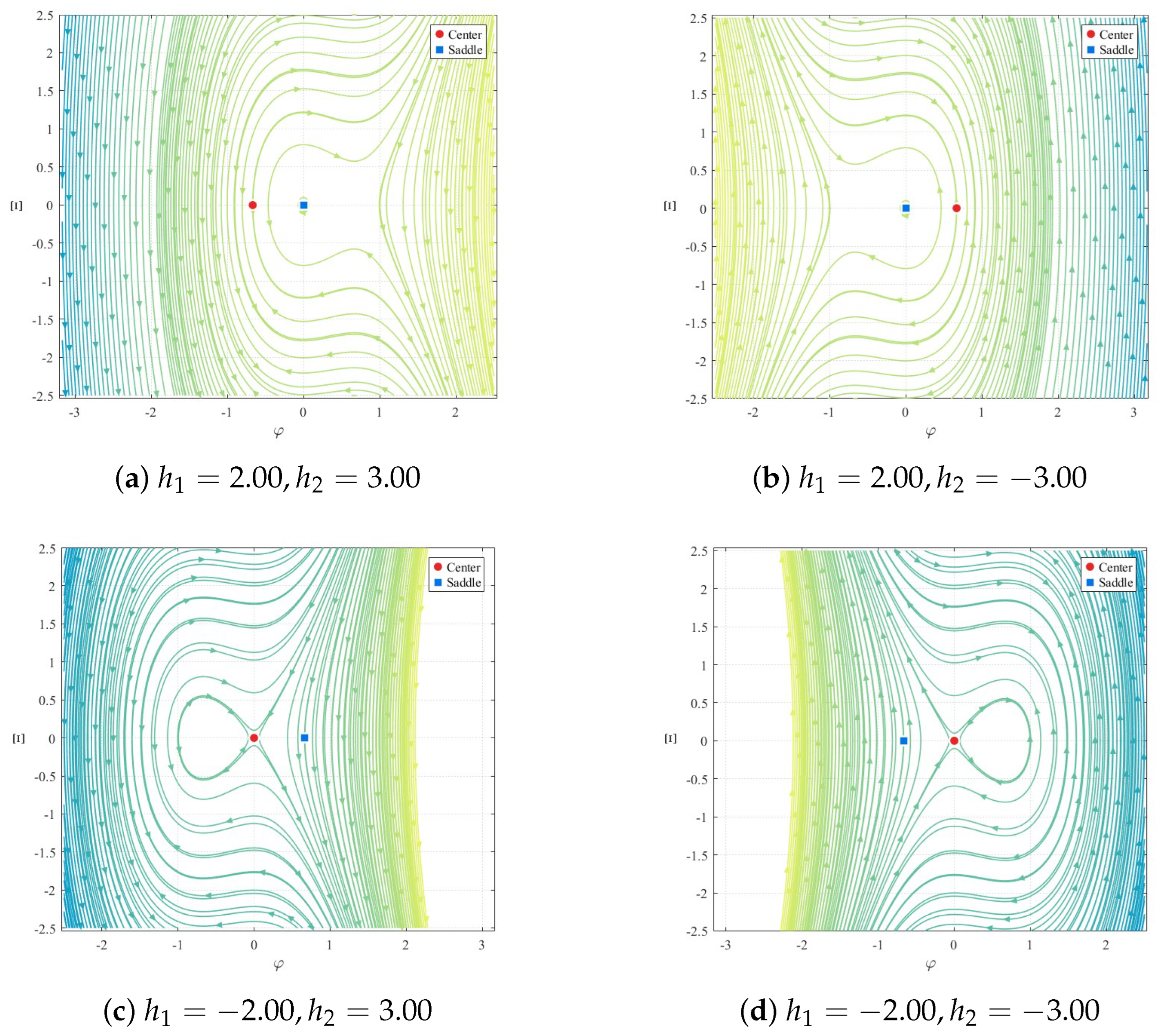
Its characteristic polynomial is ${\lambda }^2-(h_1+2h_2{\phi }_e)=0$, so the eigenvalues are ${\lambda }_{\pm }=\pm \sqrt{h_1+2h_2{\phi }_e}$. Accordingly, the equilibrium is a saddle when $h_1+2h_2{\phi }_e>0$, and a center when $h_1+2h_2{\phi }_e<0$. Figure 1 illustrates the phase space, and the organization of the phase space can now be described more precisely.

• If $h_1>0$: O is a saddle and E is a center. In this case, $h_{*}<0$, and the interval $h_{*}<h<0$ constitutes the bounded-wave window. Each level set in this range is a closed orbit enclosing the center E and therefore represents a bounded periodic orbit in the $(\phi ,\Xi )$-phase plane. The corresponding traveling-wave field U becomes periodic only after reconstructing $U_{\xi }=\phi$ and imposing the zero-mean condition over one oscillation period. The singular level $h=0$ is a homoclinic loop attached to the saddle O, which corresponds to a solitary-wave threshold. For $h<h_{*}$ or $h>0$, the level curves are open, and no bounded traveling-wave profile is generated.
• If $h_1<0$, the nature of the equilibria is reversed: O becomes a center, and E becomes a saddle. Here $h_{*}>0$, and the interval $0<h<h_{*}$ produces a family of closed periodic trajectories around the origin in the $(\phi ,\Xi )$-plane. The periodicity of the original field U requires an additional reconstruction condition. The critical level $h=h_{*}$ gives a homoclinic loop based at E, whereas all remaining levels correspond to open branches.
• If $h_1=0$ (the transition value), the configuration of the two equilibrium points collapses into a degenerate structure. This marks the boundary between the two phase diagrams with the different topological properties described above.

The first integral not only expresses energy conservation but also explicitly partitions the reduced system (in terms of parameters) into periodic, separatrix (solitary-wave threshold), and unbounded regimes. It should be emphasized that closed and homoclinic orbits in the $(\phi ,\Xi )$-plane describe the dynamics of the gradient variable $\phi =U_{\xi }$. The original traveling-wave field is reconstructed by

$$U\left(\xi \right)=U_0+{\int }_{{\xi }_0}^{\xi }\phi \left(s\right)ds.$$

(15)

If $\phi$ is periodic with period T, then

$$U(\xi +T)-U\left(\xi \right)={\int }_{\xi }^{\xi +T}\phi \left(s\right)ds.$$

(16)

Therefore, the reconstructed field U is T-periodic if and only if

$${\int }_0^T\phi \left(s\right)ds=0.$$

(17)

If this zero-mean condition is not satisfied, U contains a nonzero drift over each period, although $\phi$ itself remains periodic. Similarly, for a homoclinic gradient profile, the integral of $\phi$ over the real line gives the jump of the reconstructed field U. Hence a nonzero integral corresponds to a kink/antikink-type reconstructed field rather than a localized pulse.

2.3. Closed-Form Separatrices and Their Wave Interpretation

The homoclinic orbit is written explicitly in both saddle regimes. The separatrix corresponds to the critical energy level of the planar Hamiltonian system at which an orbit connects a saddle equilibrium to itself, thereby marking the threshold for localized solitary-wave formation.

Case 1: $h_1>0$ (Saddle at the origin, $h=0$)

For $h_1>0$, the separatrix is attached to the origin at $h=0$. Direct integration yields the closed-form homoclinic solution

$${\phi }_h\left(\xi \right)=-{\displaystyle \frac{3h_1}{2h_2}}{sech}^2\left({\displaystyle \frac{\sqrt{h_1}}{2}}(\xi -{\xi }_0)\right).$$

(18)

Differentiation of ${\phi }_h\left(\xi \right)$ with respect to $\xi$ leads to

$${\Xi }_h\left(\xi \right)={\displaystyle \frac{3h_1\sqrt{h_1}}{2h_2}}{sech}^2\left({\displaystyle \frac{\sqrt{h_1}}{2}}(\xi -{\xi }_0)\right)tanh\left({\displaystyle \frac{\sqrt{h_1}}{2}}(\xi -{\xi }_0)\right),$$

(19)

which gives the tangent component ${\Xi }_h\left(\xi \right)$ of the homoclinic orbit in the $(\phi ,\Xi )$-phase plane. Since $\phi =U_{\xi }$, the corresponding traveling-wave field in the original PDE variable is obtained by one further integration

$$U_h\left(\xi \right)=U_0-{\displaystyle \frac{3\sqrt{h_1}}{h_2}}tanh\left({\displaystyle \frac{\sqrt{h_1}}{2}}(\xi -{\xi }_0)\right).$$

(20)

Thus, in the original field variable U, the reconstructed profile is of kink/antikink type rather than a bell-shaped pulse.

Case 2: $h_1<0$ (Shifted saddle, $h=h_{*}$)

For $h_1<0$, the homoclinic loop is attached to the shifted saddle E at the critical energy $h_{*}=-{\displaystyle \frac{h_1^3}{6h_2^2}}$. A parallel integration procedure gives:

$${\phi }_h\left(\xi \right)=-{\displaystyle \frac{h_1}{h_2}}+{\displaystyle \frac{3h_1}{2h_2}}{sech}^2\left({\displaystyle \frac{\sqrt{-h_1}}{2}}(\xi -{\xi }_0)\right).$$

(21)

Differentiation with respect to $\xi$ then results in

$${\Xi }_h\left(\xi \right)=-{\displaystyle \frac{3h_1\sqrt{-h_1}}{2h_2}}{sech}^2\left({\displaystyle \frac{\sqrt{-h_1}}{2}}(\xi -{\xi }_0)\right)tanh\left({\displaystyle \frac{\sqrt{-h_1}}{2}}(\xi -{\xi }_0)\right).$$

(22)

Reconstructing the original field variable from $\phi =U_{\xi }$ yields

$$U_h\left(\xi \right)=U_0-{\displaystyle \frac{h_1}{h_2}}(\xi -{\xi }_0)+{\displaystyle \frac{3h_1}{h_2\sqrt{-h_1}}}tanh\left({\displaystyle \frac{\sqrt{-h_1}}{2}}(\xi -{\xi }_0)\right),$$

(23)

which contains a linear secular term and therefore does not represent a spatially localized pulse of the original field U.

Consequently, the waveform transition in the extended KP model is controlled by which equilibrium plays the role of the saddle and which energy level acts as the separatrix threshold.

3. Periodic Forcing, Separatrix Splitting, and Sensitivity

3.1. Periodically Forced Reduced System

In real physical systems, wave motion is often influenced by external periodic forces. To probe structural stability, a small periodic forcing term $\mu cos\left(\omega \xi \right)$ is added to the right-hand side of the $\Xi$-equation. The corresponding perturbed system is defined as

$$\left\{\begin{array}{c}{\displaystyle \frac{d\phi }{d\xi }}=\Xi ,\hfill \\ {\displaystyle \frac{d\Xi }{d\xi }}=h_1\phi \left(\xi \right)+h_2{\phi }^2\left(\xi \right)+\mu cos\left(\omega \xi \right),\hfill \end{array}\right.$$

(24)

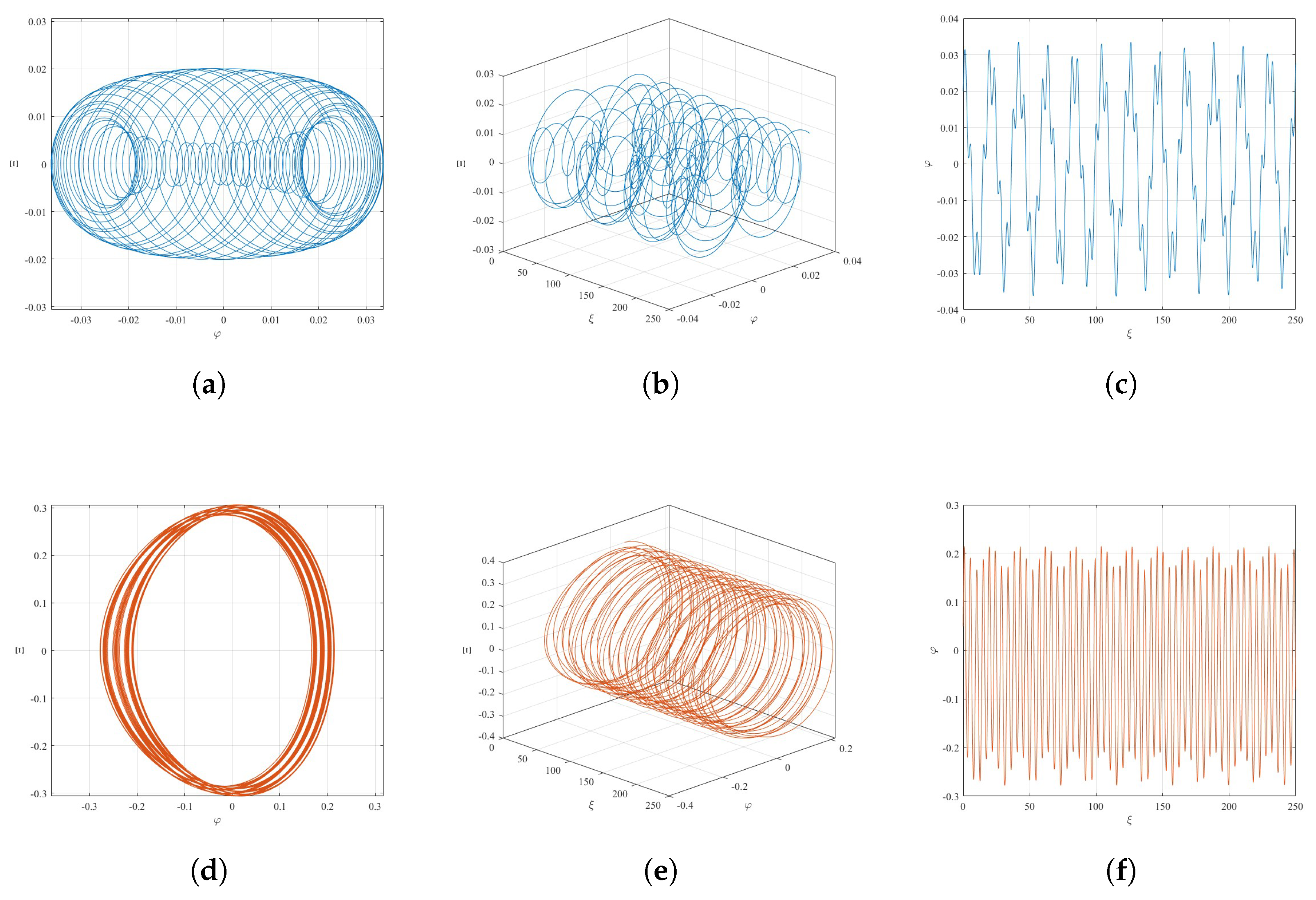
where $\mu$ denotes the perturbation amplitude and $\omega$ the frequency, with $0<\mu \ll 1$. To examine the dynamical behavior of the perturbed system, Figure 2 presents the evolution under different choices of $\mu$ and $\omega$, with the remaining parameters fixed at $h_1=-2$, $h_2=-3$ and initial conditions $\phi \left(0\right)=0.1$, $\Xi \left(0\right)=0.2$.

3.2. Harmonic Forcing and Separatrix Splitting

To complement the numerical phase portraits in Section 2, an analytical criterion for the onset of chaos in the periodically forced model (24) is now derived.

Let ${\Gamma }_h$ denote the homoclinic orbit of the unperturbed system corresponding to (18), (19), (21) and (22). The Melnikov function, which measures the separation between the stable and unstable manifolds, is defined as

$$M\left({\xi }_0\right)=\mu {\int }_{-\infty }^{\infty }{\Xi }_h\left(\tau \right)cos\left(\omega (\tau +{\xi }_0)\right)d\tau .$$

(25)

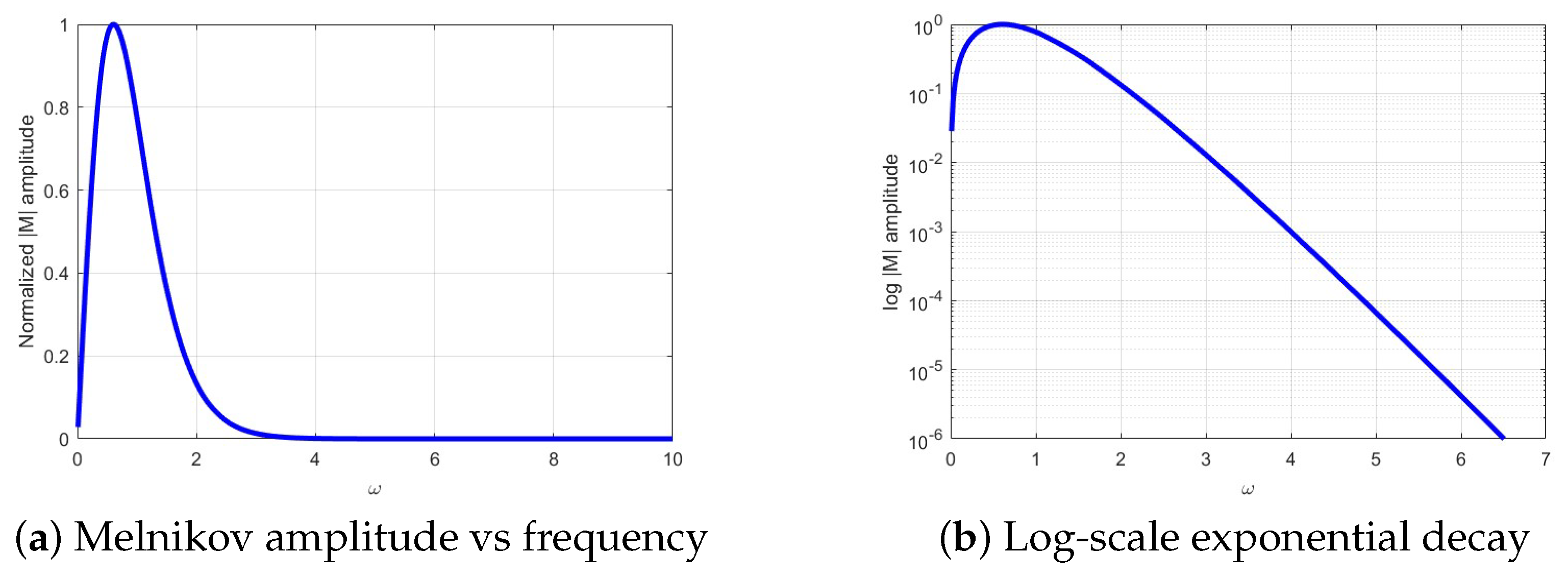
The Melnikov function amplitude $\left|M\right(\omega \left)\right|$ exhibits a resonant peak followed by an exponential decay with increasing perturbation frequency $\omega$, as illustrated in Figure 3.

A direct calculation yields

$$M\left({\xi }_0\right)=\pm \mu A\left(\omega \right)sin\left(\omega {\xi }_0\right),A\left(\omega \right)={\displaystyle \frac{6\pi {\omega }^2}{\left|h_2\right|sinh\left(\frac{\pi \omega }{\sqrt{|h_1|}}\right)}}>0,$$

(26)

where the overall sign depends on the orientation of the chosen homoclinic branch and is immaterial for the simple-zero criterion. For large $\omega$, the Melnikov amplitude factor $A\left(\omega \right)$ decays exponentially. Hence, the splitting distance, which is proportional to $\mu A\left(\omega \right)$, becomes exponentially small in the high-frequency regime. Therefore, the exponential factor does not merely restate that the perturbation amplitude $\mu$ is small; rather, it shows that high-frequency forcing produces an exponentially small separatrix splitting, although the Melnikov function still has simple zeros for $\omega \ne 0$.

Because the two types of homoclinic orbits have different forms of the constant offset term and radical term, Equation (26) cannot be directly applied to the positive and negative cases of $h_1$, so we consider the Mernikov analytic formula in different cases.

When $h_1>0$, the homoclinic orbit of the undisturbed system is given by Equation (18). Since the integration result is independent of the constant phase ${\xi }_0$, it can be taken as ${\xi }_0=0$, which is simplified as:

$${\phi }_h\left(\xi \right)=-{\displaystyle \frac{3h_1}{2h_2}}{\mathrm{sech}}^2\left({\displaystyle \frac{\sqrt{h_1}}{2}}\xi \right).$$

(27)

Define $\Xi ={\displaystyle \frac{d\phi }{d\xi }}$ according to the phase plane variable, and find the derivative of Equation (18) about $\xi$:

$$\begin{array}{cc}\hfill X{i}_h\left(\xi \right)={\displaystyle \frac{d{\phi }_h}{d\xi }}& =-{\displaystyle \frac{3h_1}{2h_2}}·2\mathrm{sech}\left({\displaystyle \frac{\sqrt{h_1}}{2}}\xi \right)·\left(-\mathrm{sech}\left({\displaystyle \frac{\sqrt{h_1}}{2}}\xi \right)tanh\left({\displaystyle \frac{\sqrt{h_1}}{2}}\xi \right)\right)·{\displaystyle \frac{\sqrt{h_1}}{2}}\hfill \\ & ={\displaystyle \frac{3h_1\sqrt{h_1}}{2h_2}}{\mathrm{sech}}^2\left({\displaystyle \frac{\sqrt{h_1}}{2}}\xi \right)tanh\left({\displaystyle \frac{\sqrt{h_1}}{2}}\xi \right).\hfill \end{array}$$

(28)

Substitute ${\Xi }_h\left(\xi \right)$ into the Melnikov integral Equation (26) to obtain

$$\begin{array}{cc}\hfill M\left({\xi }_0\right)& =\mu {\int }_{-\infty }^{\infty }{\Xi }_h\left(\xi \right)cos\left(\omega \left(\xi +{\xi }_0\right)\right)d\xi \hfill \\ & =\mu cos\left(\omega {\xi }_0\right){\int }_{-\infty }^{\infty }{\Xi }_h\left(\xi \right)cos\left(\omega \xi \right)d\xi +\mu sin\left(\omega {\xi }_0\right){\int }_{-\infty }^{\infty }{\Xi }_h\left(\xi \right)sin\left(\omega \xi \right)d\xi .\hfill \end{array}$$

(29)

Because ${\int }_{-\infty }^{\infty }{\Xi }_h\left(\xi \right)cos\left(\omega \xi \right)d\xi =0$, the amplitude is defined as:

$$A\left(\omega \right)={\int }_{-\infty }^{\infty }{\Xi }_h\left(\xi \right)sin\left(\omega \xi \right)d\xi .$$

(30)

Let $u={\displaystyle \frac{\sqrt{h_1}}{2}}\xi$, then $\xi ={\displaystyle \frac{2u}{\sqrt{h_1}}}$, $d\xi ={\displaystyle \frac{2du}{\sqrt{h_1}}}$ is substituted into the amplitude integral and simplified

$$A\left(\omega \right)={\displaystyle \frac{3h_1}{h_2}}{\int }_{-\infty }^{\infty }tanhu{\mathrm{sech}}^{2}usin\left({\displaystyle \frac{2\omega u}{\sqrt{h_1}}}\right)du={\displaystyle \frac{6\pi {\omega }^2}{|h_2|sinh\left(\frac{\pi \omega }{\sqrt{|h_1|}}\right)}}.$$

(31)

When $h_1<0$, the homoclinic orbit of the undisturbed system is given by Equation (21). Since the integration result is independent of the constant phase ${\xi }_0$, it can be taken as ${\xi }_0=0$, which is simplified as:

$${\phi }_h\left(\xi \right)=-{\displaystyle \frac{h_1}{h_2}}+{\displaystyle \frac{3h_1}{2h_2}}{\mathrm{sech}}^2\left({\displaystyle \frac{\sqrt{-h_1}}{2}}\xi \right).$$

(32)

According to the definition of the phase plane variable $\Xi ={\displaystyle \frac{d\phi }{d\xi }}$, differentiate Equation (21) with respect to $\xi$.

$${\Xi }_h\left(\xi \right)={\displaystyle \frac{d{\phi }_h}{d\xi }}=-{\displaystyle \frac{3h_1\sqrt{-h_1}}{2h_2}}{\mathrm{sech}}^2\left({\displaystyle \frac{\sqrt{-h_1}}{2}}\xi \right)tanh\left({\displaystyle \frac{\sqrt{-h_1}}{2}}\xi \right).$$

(33)

Substitute ${\Xi }_h\left(\xi \right)$ into the Melnikov integral Equation (25) to obtain

$$\begin{array}{cc}\hfill M\left({\xi }_0\right)& =\mu {\int }_{-\infty }^{\infty }{\Xi }_h\left(\xi \right)cos\left(\omega \left(\xi +{\xi }_0\right)\right)d\xi \hfill \\ & =\mu cos\left(\omega {\xi }_0\right){\int }_{-\infty }^{\infty }{\Xi }_h\left(\xi \right)cos\left(\omega \xi \right)d\xi +\mu sin\left(\omega {\xi }_0\right){\int }_{-\infty }^{\infty }{\Xi }_h\left(\xi \right)sin\left(\omega \xi \right)d\xi .\hfill \end{array}$$

(34)

Because ${\int }_{-\infty }^{\infty }{\Xi }_h\left(\xi \right)cos\left(\omega \xi \right)d\xi =0$, the amplitude is defined as:

$$A\left(\omega \right)={\int }_{-\infty }^{\infty }{\Xi }_h\left(\xi \right)sin\left(\omega \xi \right)d\xi .$$

(35)

Let $u={\displaystyle \frac{\sqrt{-h_1}}{2}}\xi$; then $\xi ={\displaystyle \frac{2u}{\sqrt{-h_1}}}$, $d\xi ={\displaystyle \frac{2du}{\sqrt{-h_1}}}$ is substituted into the amplitude integral and simplified to obtain

$$A\left(\omega \right)={\displaystyle \frac{3h_1}{h_2}}{\int }_{-\infty }^{\infty }tanhu{\mathrm{sech}}^{2}usin\left({\displaystyle \frac{2\omega u}{\sqrt{-h_1}}}\right)du={\displaystyle \frac{6\pi {\omega }^2}{|h_2|sinh\left(\frac{\pi \omega }{\sqrt{|h_1|}}\right)}}.$$

(36)

Consequently, the zeros of the Melnikov function are given by

$$M\left({\xi }_0\right)=0⟺{\xi }_0={\displaystyle \frac{n\pi }{\omega }},n\in \mathbb{Z}.$$

(37)

Moreover,

$${\displaystyle \frac{dM}{d{\xi }_0}}=\pm \mu A\left(\omega \right)\omega cos\left(\omega {\xi }_0\right),$$

(38)

and hence ${\displaystyle \frac{dM}{d{\xi }_0}}\ne 0$ at every zero whenever $\omega \ne 0$. Thus all zeros of M are simple. It follows that, for sufficiently small $0<\mu \ll 1$, the perturbed stable and unstable manifolds intersect transversely. By the Smale–Birkhoff homoclinic theorem (Theorem 26.1.1 in [36]), the period-$2\pi /\omega$ Poincaré map possesses a horseshoe, implying chaotic dynamics in a neighborhood of the unperturbed separatrix. The classical Melnikov method is developed in [37], and the rigorous transversality and chaos criteria can be found in Chapter 12 in [38]. For large $\omega$, the Melnikov amplitude factor $A\left(\omega \right)$ decays exponentially. Since the leading-order separatrix splitting is proportional to $\mu A\left(\omega \right)$, the splitting distance becomes exponentially small in the high-frequency regime. Thus, high-frequency forcing produces only a weak observable separation between the stable and unstable manifolds, although the Melnikov function still has simple zeros for $\omega \ne 0$.

3.3. Numerical Validation and Sensitivity

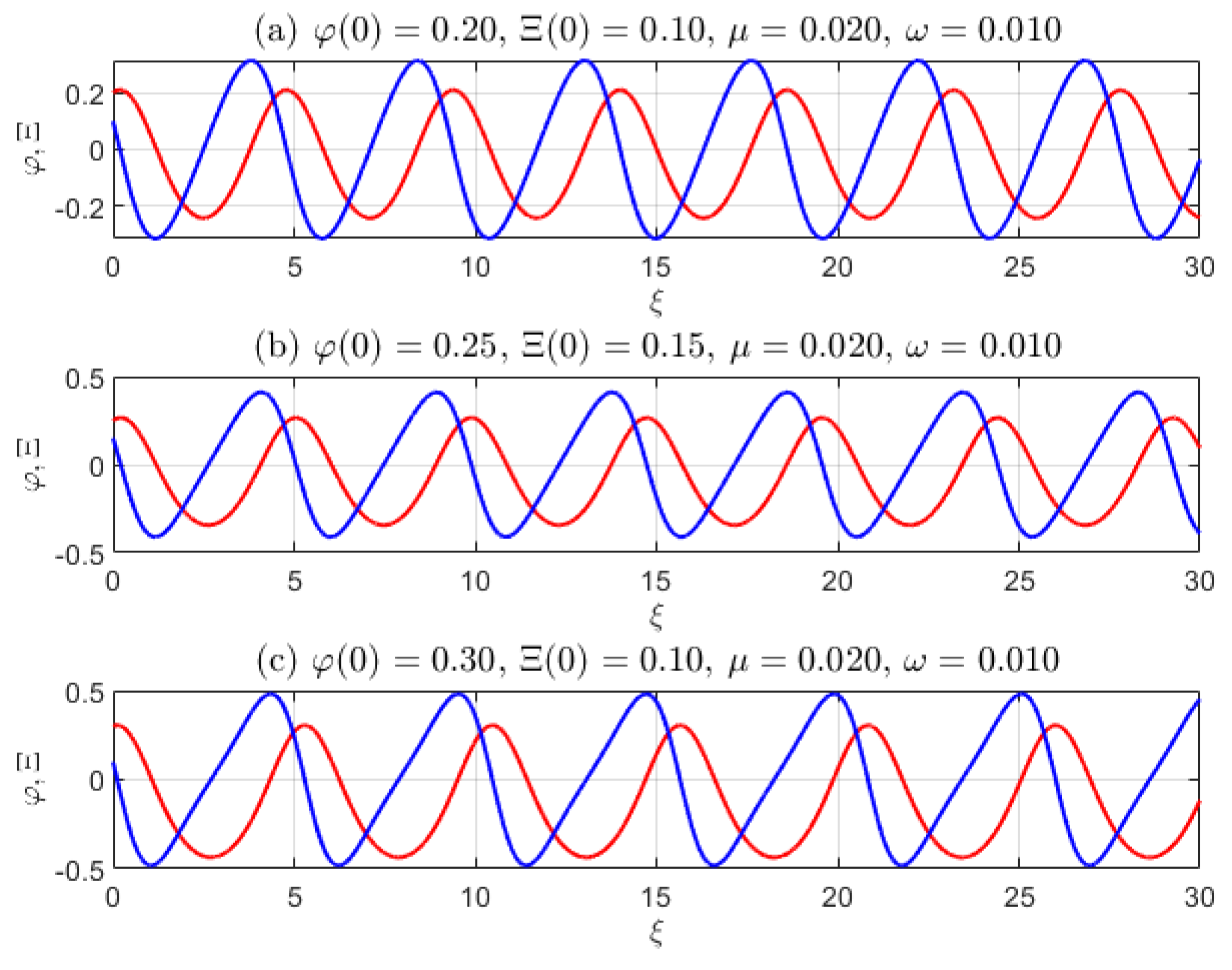
Numerical simulations are carried out for the reduced system with parameters $h_1=-2$ and $h_2=-3$, using three sets of nearby initial conditions: $\left(\phi \right(0),\Xi (0\left)\right)=(0.2,0.1)$, $(0.25,0.15)$, and $(0.3,0.1)$. In each subplot, the blue line represents the evolution profile of $\phi \left(\xi \right)$, while the red line denotes the evolution profile of $\Xi \left(\xi \right)$. Evolution profiles (see Figure 4) illustrate the response characteristics near and away from the separatrix layer.

Strong sensitivity to initial conditions appears in the vicinity of the separatrix, which is consistent with the transverse intersection of stable and unstable manifolds after separatrix splitting. In contrast, weak sensitivity to initial variations is observed away from the separatrix layer, where invariant curves persist under weak perturbations and preserve regular quasi-periodic motion.

4. Exact Solutions of the Reduced Gradient Equation

This section presents exact solutions of the reduced gradient equation $\phi \left(\xi \right)=U_{\xi }\left(\xi \right)$ in Equation (10) using the complete discriminant system. The corresponding field $U\left(\xi \right)$ is obtained by one further quadrature and must be interpreted subject to the reconstruction conditions discussed above. Starting from the Hamiltonian identity Equation (13), the coefficients are defined as

$$a={\displaystyle \frac{2h_2}{3}},b=h_1,d=2h.$$

(39)

Substituting these coefficients into Equation (13) yields ${\left({\phi }^{\prime }\right)}^2=a{\phi }^3+b{\phi }^2+d$. Applying the linear transformation $\phi =\lambda \Phi +\eta$ then gives

$${\left({\Phi }^{\prime }\right)}^2=a\lambda {\Phi }^3+(3a\eta +b){\Phi }^2+{\displaystyle \frac{3a{\eta }^2+2b\eta }{\lambda }}\Phi +{\displaystyle \frac{a{\eta }^3+b{\eta }^2+d}{{\lambda }^2}}.$$

(40)

Comparing Equation (40) with the standard form ${\left({\Phi }^{\prime }\right)}^2={\Phi }^3+{\chi }_1\Phi +{\chi }_0$ gives the following relations for the parameters

$$\lambda ={\displaystyle \frac{1}{a}},\eta =-{\displaystyle \frac{b}{3a}},{\chi }_0={\displaystyle \frac{2b^3}{27}}+a^{2}d,{\chi }_1=-{\displaystyle \frac{b^2}{3}}.$$

(41)

Therefore, the integral expression of ${\left({\Phi }^{\prime }\right)}^2={\Phi }^3+{\chi }_1\Phi +{\chi }_0$ is

$$\pm (\xi -{\xi }_0)=\int {\displaystyle \frac{d\Phi }{\sqrt{{\Phi }^3+{\chi }_1\Phi +{\chi }_0}}},$$

(42)

where $g(\Phi )={\Phi }^3+{\chi }_1\Phi +{\chi }_0$, and the third-order complete discriminant is

$$\Delta =-27{\chi }_0^2-4{{\chi }_1}^3=-27{({\displaystyle \frac{2b^3}{27}}+a^{2}d)}^2-4{(-{\displaystyle \frac{b^2}{3}})}^3=-27a^4{d}^2-4a^2{b}^{3}d.$$

(43)

Classification of solutions is then performed according to the sign of $\Delta$ and the roots of the cubic polynomial.

Case 1: $\Delta =0$, ${\chi }_1<0$

If $g(\Phi )=0$ has a double real root and a single real root, then $g(\Phi )={(\Phi -{\delta }_1)}^2(\Phi -{\delta }_2)$, where ${\delta }_1\ne {\delta }_2$. Thus, when $\Phi >{\delta }_1$, Equation (42) can be rewritten as

$$\pm (\xi -{\xi }_0)=\int {\displaystyle \frac{d\Phi }{(\Phi -{\delta }_1)\sqrt{\Phi -{\delta }_2}}}=\left\{\begin{array}{cc}{\displaystyle \frac{1}{\sqrt{{\delta }_1-{\delta }_2}}ln\left|\frac{\sqrt{\Phi -{\delta }_2}-\sqrt{{\delta }_1-{\delta }_2}}{\sqrt{\Phi -{\delta }_2}+\sqrt{{\delta }_1-{\delta }_2}}\right|,}\hfill & {\delta }_1>{\delta }_2.\hfill \\ {\displaystyle \frac{2}{\sqrt{{\delta }_2-{\delta }_1}}arctan\frac{\sqrt{\Phi -{\delta }_2}}{\sqrt{{\delta }_2-{\delta }_1}},}\hfill & {\delta }_1<{\delta }_2.\hfill \end{array}\right.$$

(44)

Integrating Equation (44) yields the following solution branches of the reduced gradient Equation (10):

$${\phi }_1(x,y,z,t)=\lambda \left\{({\delta }_1-{\delta }_2){tanh}^2\left[{\displaystyle \frac{\sqrt{{\delta }_1-{\delta }_2}}{2}}(\xi -{\xi }_0)\right]+{\delta }_2\right\}+\eta .$$

(45)

$${\phi }_2(x,y,z,t)=\lambda \left\{({\delta }_1-{\delta }_2){coth}^2\left[{\displaystyle \frac{\sqrt{{\delta }_1-{\delta }_2}}{2}}(\xi -{\xi }_0)\right]+{\delta }_2\right\}+\eta .$$

(46)

$${\phi }_3(x,y,z,t)=\lambda \left\{(-{\delta }_1+{\delta }_2){tan}^2\left[{\displaystyle \frac{\sqrt{-{\delta }_1+{\delta }_2}}{2}}(\xi -{\xi }_0)\right]+{\delta }_2\right\}+\eta .$$

(47)

Case 2: $\Delta =0$, ${\chi }_1=0$

If $g(\Phi )=0$ has triple real roots, then $g(\Phi )={(\Phi -\tau )}^3$. By substituting $g(\Phi )={(\Phi -\tau )}^3$ into Equation (42), the following solution branches of the reduced gradient Equation (10) can be obtained as follows:

$$\pm (\xi -{\xi }_0)=-{\displaystyle \frac{2}{\sqrt{\Phi -\tau }}}.$$

(48)

A further calculation then gives

$${\phi }_4(x,y,z,t)=\lambda \left[{\displaystyle \frac{4}{{(\xi -{\xi }_0)}^2}}+\tau \right]+\eta .$$

(49)

Case 3: $\Delta >0$, ${\chi }_1<0$

If $g(\Phi )=0$ has three different real roots ${\mu }_1$,${\mu }_2$ and ${\mu }_3$, then $g(\Phi )=(\Phi -{\mu }_1)(\Phi -{\mu }_2)(\Phi -{\mu }_3)$, where ${\mu }_1<{\mu }_2<{\mu }_3$. When ${\mu }_1<\Phi <{\mu }_2$, a new transformation is considered:

$$\Phi ={\mu }_1+({\mu }_2-{\mu }_1){sin}^2\theta .$$

(50)

From Equation (42), the following is obtained:

$$\begin{array}{cc}\hfill \pm (\xi -{\xi }_0)& ={\displaystyle \frac{2({\mu }_2-{\mu }_1)sin\theta cos\theta d\theta }{\sqrt{{({\mu }_2-{\mu }_1)}^2{sin}^2\theta {cos}^2\theta ·({\mu }_3-{\mu }_1)\left[1-\frac{{\mu }_2 - {\mu }_1}{{\mu }_3 - {\mu }_1}{sin}^2\theta \right]}}}\hfill \\ & ={\displaystyle \frac{2}{\sqrt{{\mu }_3-{\mu }_1}}}\int {\displaystyle \frac{d\theta }{\sqrt{1-{\chi }^2{sin}^2\theta }}},\hfill \end{array}$$

(51)

where ${\chi }^2={\displaystyle \frac{{\mu }_2-{\mu }_1}{{\mu }_3-{\mu }_1}}$, $0<{\chi }^2<1$. From Equation (42), the following solution branches of the reduced gradient Equation (10) is given by

$${\phi }_5(x,y,z,t)=\lambda \left[{\mu }_1+({\mu }_2-{\mu }_1){\mathrm{sn}}^2\left({\displaystyle \frac{\sqrt{{\mu }_3-{\mu }_1}}{2}}(\xi -{\xi }_0),\chi \right)\right]+\eta ,$$

(52)

let

$$\alpha ={\displaystyle \frac{\sqrt{{\mu }_3-{\mu }_1}}{2}},\nu =\alpha (\xi -{\xi }_0),$$

(53)

Since the period of ${sn}^2(\nu ,\chi )$ in $\nu$ is $2K\left(\chi \right)$, the period of ${\phi }_5$ is

$$T_5={\displaystyle \frac{2K\left(\chi \right)}{\alpha }}={\displaystyle \frac{4K\left(\chi \right)}{\sqrt{{\mu }_3-{\mu }_1}}},$$

(54)

where $K\left(\chi \right)$ is the complete elliptic integral of the first kind. Using

$${\int }_0^{2K\left(\chi \right)}{sn}^2(\nu ,\chi )d\nu ={\displaystyle \frac{2\left[K\right(\chi )-E(\chi \left)\right]}{{\chi }^2}},$$

(55)

where $E\left(\chi \right)$ is the complete elliptic integral of the second kind. The mean value of ${\phi }_5$ over one period is

$$\overline{{\phi }_5}=\lambda \left[{\mu }_1+({\mu }_2-{\mu }_1){\displaystyle \frac{K\left(\chi \right)-E\left(\chi \right)}{{\chi }^{2}K\left(\chi \right)}}\right]+\eta .$$

(56)

Consequently,

$$U_5(\xi +T_5)-U_5\left(\xi \right)={\int }_{\xi }^{\xi +T_5}{\phi }_5\left(s\right)ds=T_5{\overline{\phi }}_5.$$

(57)

Thus, the reconstructed field $U_5$ is periodic if and only if ${\overline{\phi }}_5=0$, namely,

$$\lambda \left[{\mu }_1+({\mu }_2-{\mu }_1){\displaystyle \frac{K\left(\chi \right)-E\left(\chi \right)}{{\chi }^{2}K\left(\chi \right)}}\right]+\eta =0.$$

(58)

If this condition is not satisfied, ${\phi }_5$ remains a periodic gradient profile, whereas the reconstructed field $U_5$ contains a nonzero drift over one period.

When $\Phi >{\mu }_3$, the transformation is considered

$$\Phi ={\displaystyle \frac{-{\mu }_2{sin}^2\theta +{\mu }_3}{{cos}^2\theta }}.$$

(59)

Substituting this expression yields

$$\begin{array}{cc}\hfill \pm (\xi -{\xi }_0)& ={\displaystyle \frac{2({\mu }_3-{\mu }_2)sin\theta }{{cos}^3\theta }}·{\displaystyle \frac{{cos}^6\theta }{{({\mu }_3-{\mu }_2)}^2({\mu }_3-{\mu }_1)\left[1-{\displaystyle \frac{{\mu }_2-{\mu }_1}{{\mu }_3-{\mu }_1}}{sin}^2\theta \right]{sin}^2\theta }}d\theta \hfill \\ \hfill & ={\displaystyle \frac{2}{\sqrt{{\mu }_3-{\mu }_1}}}\int {\displaystyle \frac{d\theta }{\sqrt{1-{\rho }^2{sin}^2\theta }}}.\hfill \end{array}$$

(60)

The following solution branches of the reduced gradient Equation (10) are given by

$${\phi }_6(x,y,z,t)=\lambda \left[{\displaystyle \frac{{\mu }_3-{\mu }_2{\mathrm{sn}}^2\left(\frac{\sqrt{{\mu }_3-{\mu }_1}}{2}(\xi -{\xi }_0),\rho \right)}{{\mathrm{cn}}^2\left(\frac{\sqrt{{\mu }_3-{\mu }_1}}{2}(\xi -{\xi }_0),\rho \right)}}\right]+\eta ,$$

(61)

where ${\rho }^2={\displaystyle \frac{{\mu }_2-{\mu }_1}{{\mu }_3-{\mu }_1}}$.

Case 4: $\Delta <0$

If $g(\Phi )=0$ has only one real root $\kappa$, then $g(\Phi )=(\Phi -\kappa )({\Phi }^2+p\Phi +q)$, where $p^2-4q<0$. For $\Phi >\kappa$, set $\Phi =\kappa +\sqrt{{\kappa }^2+p\kappa +q}{tan}^2{\displaystyle \frac{\theta }{2}}$. Equation (44) then yields

$$\begin{array}{cc}\hfill \pm (\xi -{\xi }_0)& =\int {\displaystyle \frac{d\Phi }{\sqrt{(\Phi -\kappa )({\Phi }^2+p\Phi +q)}}}\hfill \\ \hfill & =\int {\displaystyle \frac{\sqrt{{\kappa }^2+p\kappa +q}tan\frac{\theta }{2}{sec}^2\frac{\theta }{2}d\theta }{{({\kappa }^2+p\kappa +q)}^{3/4}tan\frac{\theta }{2}{sec}^2\frac{\theta }{2}\sqrt{1-{\varrho }^2{sin}^2\theta }}}\hfill \\ \hfill & ={\displaystyle \frac{1}{{({\kappa }^2+p\kappa +q)}^{1/4}}}\int {\displaystyle \frac{d\theta }{\sqrt{1-{\varrho }^2{sin}^2\theta }}},\hfill \end{array}$$

(62)

where ${\varrho }^2={\displaystyle \frac{1}{2}}\left(1-{\displaystyle \frac{\kappa +\frac{p}{2}}{\sqrt{{\kappa }^2+p\kappa +q}}}\right)$. Next, let $cn({({\kappa }^2+p\kappa +q)}^{{\displaystyle \frac{1}{4}}}(\xi -{\xi }_0),\varrho )=cos\theta$. Moreover, this yields

$$cos\theta ={\displaystyle \frac{\sqrt{{\kappa }^2+p\kappa +q}}{\Phi -\kappa +\sqrt{{\kappa }^2+p\kappa +q}}}-1.$$

(63)

When $\Phi >\kappa$, the following solution branches of the reduced gradient Equation (10) are given by

$${\phi }_7(x,y,z,t)=\lambda \left[\kappa +{\displaystyle \frac{2\sqrt{{\kappa }^2+p\kappa +q}}{1+\mathrm{cn}\left({({\kappa }^2+p\kappa +q)}^{1/4}(\xi -{\xi }_0),\varrho \right)}}-\sqrt{{\kappa }^2+p\kappa +q}\right]+\eta .$$

(64)

Similarly, the following solution branches of the reduced gradient Equation (10) can also be written as

$${\phi }_8(x,y,z,t)=\lambda \left[\kappa +{\displaystyle \frac{2\sqrt{{\kappa }^2+p\kappa +q}}{1-\mathrm{cn}\left({({\kappa }^2+p\kappa +q)}^{\frac{1}{4}}(\xi -{\xi }_0),\varrho \right)}}-\sqrt{{\kappa }^2+p\kappa +q}\right]+\eta .$$

(65)

The association between these branches and the separatrix can be clarified through the Hamiltonian energy level. For $h_1>0$, the origin $O=(0,0)$ is a saddle point, and the homoclinic separatrix is located at h = 0. In the case of double roots $\Delta =0$, the branch ${\phi }_1$ is associated with the threshold of the homoclinic separation line in the $(\phi ,\Xi )$-plane. Substituting ${\phi }_1$ into the Hamiltonian yields H = 0, so it lies on the homoclinic separatrix. ${\phi }_2$ satisfies $\Phi <{\delta }_1$, and there are movable poles in the solution, which is not of practical research significance; ${\phi }_3$ corresponds to ${\delta }_1<{\delta }_2$ and belongs to the solution of bounded oscillatory trajectories outside the domain. ${\phi }_2$ contains the square of hyperbolic cotangent, while ${\phi }_3$ includes the square of tangent. The solution has finite point singularities or boundlessness and does not belong to the standard homoclinic trajectory profile. Thus, the double-root condition is necessary for the separatrix threshold, but not every branch arising from $\Delta =0$ is itself a homoclinic profile. The Jacobi elliptic solutions ${\phi }_5$–${\phi }_6$ correspond to the bounded closed-orbit families ($\Delta >0$), representing periodic traveling waves. The ${\phi }_7$ and ${\phi }_8$ derived from the non-degenerate condition $\Delta <0$ can construct elliptical gradient solutions, but the process of restoring the original field integration will produce divergent terms, making it impossible to obtain bounded physical traveling wave solutions of the original equation. The rational solution ${\phi }_4$ and the remaining branches ${\phi }_7$–${\phi }_8$ are associated with degenerate or unbounded energy levels, which do not yield bounded wave profiles.

5. Representative Wave Profiles

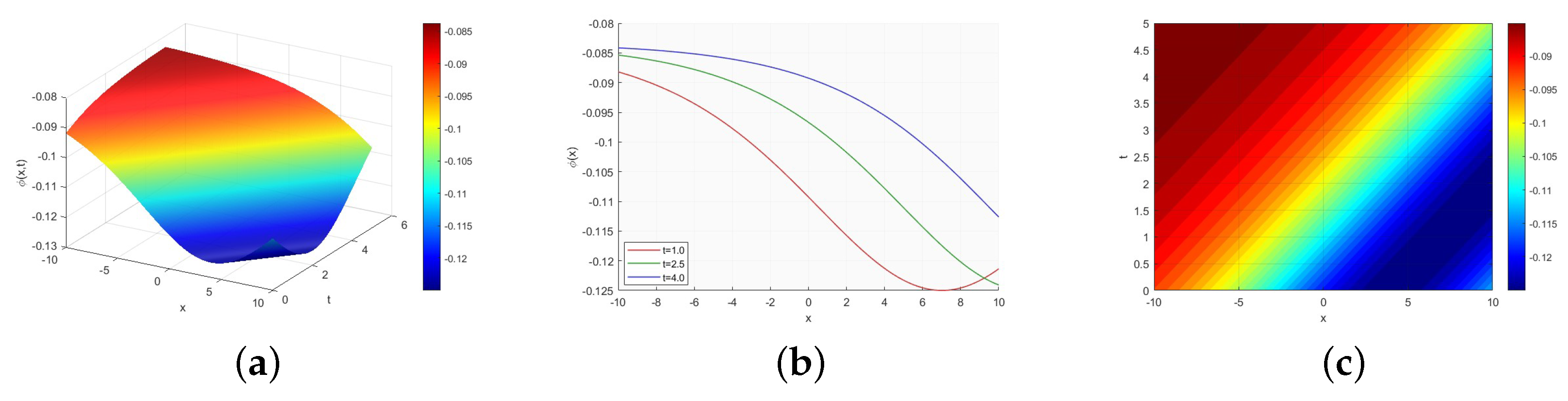
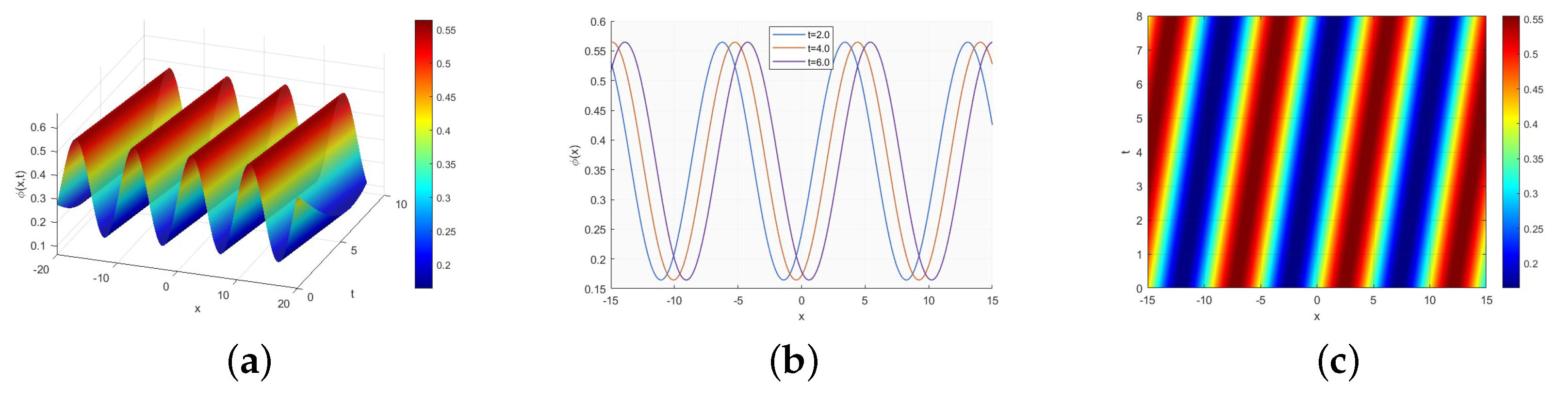
Figure 5 and Figure 6 present three-dimensional, two-dimensional, and contour maps of representative profiles of the reduced gradient variable $\phi =U_{\xi }$ governed by Equation (10). These figures should therefore be interpreted as gradient profiles rather than direct plots of the original field U. Figure 5 shows the hyperbolic homoclinic gradient profile associated with the separatrix branch. As shown by the reconstruction formula in Equation (20), the corresponding original field U is of kink/antikink type rather than a bell-shaped localized pulse. Figure 6 displays the periodic Jacobi elliptic gradient profile ${\phi }_5$. According to the reconstruction condition derived in Section 4, the original field $U_5$ is periodic only if the zero-mean condition Equation (58) is satisfied. Otherwise, Figure 6 represents a periodic gradient profile, while the reconstructed field $U_5$ contains a nonzero drift over one period.

6. Conclusions

The traveling-wave branch of the extended $(3+1)$-dimensional KP equation reduces to a Hamiltonian system. Phase-space analysis shows that bounded solutions exist regardless of the sign of $h_1$, whereas the separatrix marks the onset of solitary waves. The first integral clearly distinguishes among periodic orbits, solitary threshold orbits, and unbounded orbits. The Melnikov amplitude $A\left(\omega \right)$ decays exponentially as the forcing frequency increases (see Figure 3). Consequently, the leading-order separatrix splitting distance, proportional to $\mu A\left(\omega \right)$, becomes exponentially small in the high-frequency regime. Thus, high-frequency forcing produces only a weak observable splitting of the stable and unstable manifolds, although transverse intersections are still predicted by the simple-zero Melnikov criterion. The exact solutions obtained via the complete discriminant method are consistent with the phase-space structure of the reduced gradient system. In particular, the elliptic branch ${\phi }_5$ corresponds to a periodic closed orbit in the $(\phi ,\Xi )$-plane, while the hyperbolic branch corresponds to the separatrix limit. However, since $\phi =U_{\xi }$, a periodic gradient profile yields a periodic original field U only when its mean value over one period is zero. Otherwise, the reconstructed field contains a nonzero drift. Similarly, reconstructing U from the separatrix gradient profile shows that, when $h_1>0$, the original field exhibits a step-like kink/antikink waveform rather than a bell-shaped localized pulse. Under periodic external forcing, Melnikov analysis predicts separatrix splitting, whereas the exponential decay of the forcing amplitude with frequency implies that high-frequency effects are weak. In this regime, the system exhibits quasi-periodic and irregular responses and shows sensitivity to initial conditions. In the absence of external forcing, a comparison of solution evolutions confirms the structural stability of the system.

References

1. Swapna, Y.; Nirmale, V.; Pavani, N.; Singh, C.; Ranganathan, R.; Thontla, A.R.; Kumar, N.M. Applications of partial differential equations in fluid physics. Commun. Appl. Nonlinear Anal. 2024, 31, 207–220. [Google Scholar] [CrossRef]
2. Mohan, B.; Kumar, S. Generalization and analytic exploration of soliton solutions for nonlinear evolution equations via a novel symbolic approach in fluids and nonlinear sciences. Chin. J. Phys. 2024, 92, 10–21. [Google Scholar] [CrossRef]
3. Tang, Y.; Rezazadeh, H. On logarithmic transformation-based approaches for retrieving traveling wave solutions in nonlinear optics. Results Phys. 2023, 51, 106672. [Google Scholar] [CrossRef]
4. Liang, Y.; Wei, G.; Li, X. Painlevé integrability, similarity reductions, new soliton and soliton-like similarity solutions for the (2+1)-dimensional BKP equation. Nonlinear Dyn. 2010, 62, 195–202. [Google Scholar] [CrossRef]
5. Wang, K.; Zou, B.; Zhu, H.; Li, S.; Li, G. Phase Portrait, Bifurcation and Chaotic Analysis, Variational Principle, Hamiltonian, Novel Solitary, and Periodic Wave Solutions of the New Extended Korteweg–de Vries–Type Equation. Math. Methods Appl. Sci. 2025, 48, 9901–9909. [Google Scholar] [CrossRef]
6. Ma, W.X. Lump solutions to the Kadomtsev–Petviashvili equation. Phys. Lett. A 2015, 379, 1975–1978. [Google Scholar] [CrossRef]
7. Manukure, S.; Zhou, Y.; Ma, W.X. Lump solutions to a (2+1)-dimensional extended KP equation. Comput. Math. Appl. 2018, 75, 2414–2419. [Google Scholar] [CrossRef]
8. Kosuga, Y.; Inagaki, S.; Kawachi, Y. A fate of nonlinear evolution of drift waves: Excitation of nonlinear breathers. Phys. Plasmas 2022, 29, 122301. [Google Scholar] [CrossRef]
9. Guo, J.; He, J.; Li, M.; Mihalache, D. Exact solutions with elastic interactions for the (2+ 1)-dimensional extended Kadomtsev–Petviashvili equation. Nonlinear Dyn. 2020, 101, 2413–2422. [Google Scholar] [CrossRef]
10. Zhang, Z.; Li, B.; Chen, J.; Guo, Q.; Stepanyants, Y. Degenerate lump interactions within the Kadomtsev–Petviashvili equation. Commun. Nonlinear Sci. Numer. Simul. 2022, 112, 106555. [Google Scholar] [CrossRef]
11. Wu, H.L.; Fan, S.W.; Fei, J.X.; Ma, Z.Y. The D’Alembert type waves and the soliton molecules in a (2+ 1)-dimensional Kadomtsev-Petviashvili with its hierarchy equation. Commun. Theor. Phys. 2021, 73, 105002. [Google Scholar] [CrossRef]
12. Borluk, H.; Bruell, G.; Nilsson, D. Traveling waves and transverse instability for the fractional Kadomtsev–Petviashvili equation. Stud. Appl. Math. 2022, 149, 95–123. [Google Scholar] [CrossRef]
13. Wei, G.M.; Song, Y.X.; Xing, T.C.; Miao, S. Nonlinear waves for a variable-coefficient modified Kadomtsev–Petviashvili system in plasma physics and electrodynamics. Commun. Theor. Phys. 2025, 77, 015003. [Google Scholar] [CrossRef]
14. Ionescu, C.; Babalic, C.N.; Constantinescu, R.; Efrem, R. The functional expansion approach for solving NPDEs as a generalization of the Kudryashov and G’/G methods. Symmetry 2022, 14, 827. [Google Scholar] [CrossRef]
15. Kundu, S.; Maitra, S.; Ghosh, A. Traveling wave solution and Painleve’analysis of generalized fisher equation and diffusive Lotka–Volterra model. Int. J. Dyn. Control 2021, 9, 494–502. [Google Scholar] [CrossRef]
16. Li, Z.; Jiang, Y. Bifurcation, chaotic behavior, and traveling wave solutions for the fractional (4+ 1)-dimensional Davey–Stewartson–Kadomtsev–Petviashvili model. Open Phys. 2025, 23, 20250157. [Google Scholar] [CrossRef]
17. Ma, Y.L.; Wazwaz, A.M.; Li, B.Q. New extended Kadomtsev–Petviashvili equation: Multiple soliton solutions, breather, lump and interaction solutions. Nonlinear Dyn. 2021, 104, 1581–1594. [Google Scholar] [CrossRef]
18. Zhang, R.; Bilige, S.; Fang, T.; Chaolu, T. New periodic wave, cross-kink wave and the interaction phenomenon for the Jimbo–Miwa-like equation. Comput. Math. Appl. 2019, 78, 754–764. [Google Scholar] [CrossRef]
19. Zhu, Y.; Huang, C.; Li, J.; Zhang, R. Lump solitions, fractal soliton solutions, superposed periodic wave solutions and bright-dark soliton solutions of the generalized (3 1)-dimensional KP equation via BNNM. Nonlinear Dyn. 2024, 112, 17345–17361. [Google Scholar] [CrossRef]
20. Li, J.; Chen, C.; Zhu, Y.; Huang, C.; Zhen, X.; Zhang, R. Analytical solutions of generalized (3+ 1)-dimensional KP equation via neural network-augmented bilinear framework. Eur. Phys. J. Spec. Top. 2025, 234, 5583–5600. [Google Scholar] [CrossRef]
21. Kadomtsev, B.B.; Petviashvili, V.I. On the stability of solitary waves in weakly dispersing media. Sov. Phys. 1970, 15, 539–541. [Google Scholar]
22. Li, Y.Z.; Liu, J.G. New periodic solitary wave solutions for the new (2+ 1)-dimensional Korteweg–de Vries equation. Nonlinear Dyn. 2018, 91, 497–504. [Google Scholar] [CrossRef]
23. Yang, L.; Gao, B. The nondegenerate solitons solutions for the generalized coupled higher-order nonlinear Schrödinger equations with variable coefficients via the Hirota bilinear method. Chaos Solitons Fractals 2024, 184, 115009. [Google Scholar] [CrossRef]
24. Beenish; Samreen, M.; Alshammari, F.S. Exploring solitary wave solutions of the generalized integrable Kadomtsev–Petviashvili equation via lie symmetry and Hirota’s Bilinear method. Symmetry 2025, 17, 710. [Google Scholar] [CrossRef]
25. Schurmann, H.; Serov, V.S. Traveling wave solutions of a generalized modified Kadomtsev-Petviashvili equation. J. Math. Phys. 2004, 45, 2181–2187. [Google Scholar] [CrossRef]
26. Jie, Z.; Lin, T.; Binji, W.; Zhimin, M. Hirota condition analysis of N-solitons and their derived waves for a nonlocal (2+1)-dimensional modified Kadomtsev–Petviashvili equation. J. Math. Phys. 2025, 66, 032701. [Google Scholar] [CrossRef]
27. Nadeem, M.; Jingxia, D.; Tariq, K.U.; Alsayaad, Y. Exploring the chaotic structure and soliton solutions for (3+ 1)-dimensional generalized Kadomtsev–Petviashvili model. Sci. Rep. 2024, 14, 15865. [Google Scholar] [CrossRef]
28. Biondini, G.; Bivolcic, A.J.; Hoefer, M.A.; Moro, A. Two-dimensional reductions of the Whitham modulation system for the Kadomtsev–Petviashvili equation. Nonlinearity 2024, 37, 025012. [Google Scholar] [CrossRef]
29. Ying, L.; Li, M.; Shi, Y. New exact solutions and related dynamic behaviors of a (3+ 1)-dimensional generalized Kadomtsev–Petviashvili equation. Nonlinear Dyn. 2024, 112, 11349–11372. [Google Scholar] [CrossRef]
30. Rizvi, S.T.R.; Ahmed, N.; Ul Hassan, A. Single-layer bilinear neural network modeling of lump and multi-soliton interactions for the Kadomtsev–Petviashvili system. Eur. Phys. J. Plus 2025, 140, 1027. [Google Scholar] [CrossRef]
31. He, X.J.; Lü, X.; Li, M.G. Bäcklund transformation, Pfaffian, Wronskian and Grammian solutions to the (3+1)-dimensional generalized Kadomtsev–Petviashvili equation. Anal. Math. Phys. 2021, 11, 4. [Google Scholar] [CrossRef]
32. Al-Askar, F.M.; Cesarano, C.; Mohammed, W.W. Effects of the Wiener Process and Beta Derivative on the Exact Solutions of the Kadomtsev-Petviashvili Equation. Axioms 2023, 12, 748. [Google Scholar] [CrossRef]
33. Li, K.Q. Multiple rogue wave solutions of a generalized (3+ 1)-dimensional variable-coefficient Kadomtsev–Petviashvili equation. Open Phys. 2022, 20, 452–457. [Google Scholar] [CrossRef]
34. Alharthi, N.H.; Kaplan, M.; Alqahtani, R.T. Soliton Dynamics and Modulation Instability in the (3+1)-Dimensional Generalized Fractional Kadomtsev–Petviashvili Equation. Symmetry 2025, 17, 666. [Google Scholar] [CrossRef]
35. Guckenheimer, J.; Holmes, P. Nonlinear Oscillations, Dynamical Systems, and Bifurcations of Vector Fields; Springer Science & Business Media: Berlin/Heidelberg, Germany, 2013. [Google Scholar]
36. Wiggins, S. Introduction to Applied Nonlinear Dynamical Systems and Chaos; Springer: Berlin/Heidelberg, Germany, 2003. [Google Scholar]
37. Melnikov, V.K. On the stability of the center for time periodic perturbations. Trans. Mosc. Math. Soc. 1963, 12, 1–56. [Google Scholar]
38. Chicone, C. Homoclinic Orbits, Melnikov’s Method, and Chaos. In Ordinary Differential Equations with Applications; Springer: Berlin/Heidelberg, Germany, 2024; pp. 529–589. [Google Scholar]
Figure 1. Phase portraits of the given equation with different parameter values under consideration.
Mathematics 14 01861 g001
Figure 2. Dynamical behaviors of the forced system for h 1 = 2 , h 2 = 3 with initial conditions φ ( 0 ) = 0.1 , Ξ ( 0 ) = 0.2 . (a) Two-dimensional phase portrait. (b) Three-dimensional phase portrait. (c) Sensitivity analysis. (d) Two-dimensional phase portrait. (e) Three-dimensional phase portrait. (f) Sensitivity analysis.
Mathematics 14 01861 g002
Figure 3. Melnikov amplitude decay with respect to the forcing frequency.
Mathematics 14 01861 g003
Figure 4. Initial condition sensitivity of the reduced system for h 1 = 2 , h 2 = 3 .
Mathematics 14 01861 g004
Figure 5. Hyperbolic gradient profile φ 1 = U ξ of the reduced gradient Equation (10) for k = 2.00 , m = 1.00 , l = 2.00 , and h = 0.00 . The three-dimensional surface and contour plots are drawn at fixed z = 0 and t = 0 , while the one-dimensional cross-sections additionally use y = 0 . The reconstructed original field U is obtained by one further integration and has a kink/antikink-type profile. (a) Three-dimensional diagram. (b) Two-dimensional diagram. (c) Contour diagram.
Mathematics 14 01861 g005
Figure 6. Periodic Jacobi elliptic gradient profile φ 5 = U ξ of the reduced gradient Equation (10) for k = 0.80 , m = 0.80 , l = 0.30 , and h = 2.00 . The three-dimensional surface and contour plots are drawn at fixed z = 0 and t = 0 , while the one-dimensional cross-sections additionally use y = 0 . The reconstructed field U 5 is periodic only when the zero-mean condition over one period is satisfied. (a) Three-dimensional diagram. (b) Two-dimensional diagram. (c) Contour diagram.
Mathematics 14 01861 g006
Disclaimer/Publisher’s Note: The statements, opinions and data contained in all publications are solely those of the individual author(s) and contributor(s) and not of MDPI and/or the editor(s). MDPI and/or the editor(s) disclaim responsibility for any injury to people or property resulting from any ideas, methods, instructions or products referred to in the content.