Article

Sigmoid Comprehensive Learning Particle Swarm Optimization

School of Information Engineering, Jiangxi University of Water Resources and Electric Power, 289 Tianxiang Road, Nanchang 330099, China
*
Author to whom correspondence should be addressed.
Mathematics 2026, 14(11), 1854; https://doi.org/10.3390/math14111854
Submission received: 27 April 2026 / Revised: 18 May 2026 / Accepted: 21 May 2026 / Published: 27 May 2026
(This article belongs to the Section E1: Mathematics and Computer Science)

Abstract

As a particle swarm optimization (PSO) variant introduced in our earlier work, adaptive comprehensive learning PSO (ACLPSO) relies on two critical coefficients, i.e., the interval scaling coefficient s and the probability tradeoff coefficient v to regulate dimensional maximum velocities and per-dimension learning probabilities. ACLPSO prescribes four fixed value pairs for the two coefficients; however, no principled selection criterion exists, forcing practitioners to tune the pairs manually across different problems. This paper introduces sigmoid comprehensive learning PSO (SCLPSO), removing the need for such manual tuning by defining iterative assignment rules in which s and v evolve according to sigmoid schedules. SCLPSO also refines the tradeoff term in the per-dimension learning probability update equation to strengthen exploration capability. While prior work evaluated ACLPSO and competing PSO variants solely on sixteen classical benchmark functions, the present paper extends assessment to the congress on evolutionary computation (CEC) 2013 multimodal test suite to probe generalization more thoroughly. Experimental results demonstrate that SCLPSO identifies the global optimum or a near-optimal solution on the vast majority of test functions and consistently surpasses ACLPSO under any fixed coefficient pair.

1. Introduction

Inspired by the collective foraging behavior of birds, Kennedy and Eberhart [1] introduced particle swarm optimization (PSO) in 1995. In PSO, a swarm of particles navigates a multidimensional search space in a manner analogous to the flight of a flock of birds: each particle’s position encodes a candidate solution, and the particles iteratively share positional information to promisingly converge towards the global optimum. So far, researchers have developed numerous PSO variants aimed at improving the convergence performance and have applied them to solve a wide range of engineering optimization problems, including robot trajectory planning [2,3], unmanned aerial vehicle path planning [4], power system planning [5], topology optimization [6], and so on.
Global PSO (GPSO) is a well-known PSO variant [7,8], and most other PSO variants improve upon it. Suppose N particles are “flying” in a D-dimensional search space. With respect to GPSO, each particle i (i = 1, 2, …, N) updates its velocity Vi = (Vi,1, Vi,2, …, Vi,D) and position Pi = (Pi,1, Pi,2, …, Pi,D) on each dimension d (d = 1, 2, …, D) according to Equations (1) and (2) respectively in each iteration:
V i , d = w V i , d + c 1 r 1 B i , d P i , d   + c 2 r 2 G d P i , d
P i , d = P i , d + V i , d
where w is the inertia weight; c1 and c2 are the acceleration coefficients, both fixed at 2.0; r1 and r2 are random numbers drawn uniformly from [0, 1]; Bi = (Bi,1, Bi,2, …, Bi,D) denotes the personal best position of particle i; and G = (G1, G2, …, GD) is the global best position of the swarm. The dimensional velocity update is driven by two competing forces: the term c1r1(Bi,dPi,d), referred to as personal learning p-increment, and the term c2r2(GdPi,d) as social learning g-increment. Kennedy and Eberhart [1] showed that a dominant p-increment causes the particles to roam excessively and impedes convergence, whereas an overly large g-increment drives the swarm to collapse prematurely to a local optimum. Effective PSO therefore requires a careful balance between these two forces, which corresponds to the exploration exploitation tradeoff [9]. Exploration means broadly scanning the search space to identify regions likely to contain the global optimum, while exploitation stands for intensively refining candidate positions within those regions to locate the global optimum or a near-optimal solution.
While GPSO handles low-dimensional or unimodal problems effectively, its limited exploration capacity degrades solution quality on complex high-dimensional or multimodal problems. To address this shortcoming, Liang et al. [10] put forward comprehensive learning PSO (CLPSO), which broadens exploration by having each particle get exemplar information from multiple different individuals across different dimensions during velocity updates. The CLPSO velocity update equation is presented below:
V i , d =   w V i , d +   c r E i , d P i , d
where Ei = (Ei,1, Ei,2, …, Ei,D) is the exemplar vector of particle i. A per-particle learning probability governs whether, on each dimension, the exemplar coordinate is i’s personal best position or another particle’s personal best position. A high learning probability biases the particle towards the personal best positions of other particles, while a low probability favors its own historical best position. By allowing each dimension to independently learn from the personal best positions of different particles, CLPSO sustains swarm diversity, substantially strengthens exploration, and achieves strong results on multimodal problems. Nevertheless, prior studies have reported low convergence accuracy for CLPSO on certain unimodal functions and on some challenging multimodal problems [10,11,12].
Yu and Zhang [13] developed enhanced CLPSO (ECLPSO) to improve the exploitation capability of CLPSO. ECLPSO introduces a normative interval on each dimension and uses its width to partition the search into an early exploration phase and a subsequent exploitation phase. The lower and upper bounds of the interval are the minimum and maximum personal best coordinates of all the particles on that dimension. When the interval shrinks below a prescribed threshold, ECLPSO concludes exploration on that dimension and activates an exploitation phase in which a perturbation term is appended to the velocity update. Learning probabilities are also updated iteratively as a function of each particle’s personal best fitness rank and the fraction of dimensions that have transitioned to exploitation. Experiments by Yu and Zhang [13] confirm that ECLPSO achieves higher convergence accuracy than CLPSO on most benchmark functions. Nonetheless, exploration performance remains similarly limited: both algorithms fail to locate the global optimum or a near-optimal solution on functions such as Rosenbrock, Schwefel P1.2, shifted Schwefel P1.2, rotated Rastrigin and rotated Schwefel, indicating that the exploration exploitation balance in ECLPSO is still inadequate.
Our previously proposed adaptive CLPSO (ACLPSO) extends ECLPSO with a more balanced exploration exploitation strategy [14]. ACLPSO dynamically regulates maximum velocities, inertia weights, acceleration coefficients and learning probabilities on a per-dimension basis by monitoring changes in each dimension’s normative interval, thereby strengthening the exploration capacity of ECLPSO. Two coefficients are central to this adaptation: the interval scaling coefficient s that modulates the dimensional maximum velocity, and the probability tradeoff coefficient v that shapes the per-dimension learning probability of each particle. ACLPSO employs four prespecified fixed value pairs for s and v. Experiments in ref. [14] confirm that ACLPSO achieves a sound exploration exploitation balance—successfully identifying the global optimum or a near-optimal solution across all benchmark functions—yet no universal rule governs the selection of the most suitable pair for an arbitrary problem, making ACLPSO cumbersome to apply in practice.
Given that ACLPSO requires problem-specific manual selection of s and v, a natural question arises: can this limitation be overcome by allowing s and v to vary dynamically with iterations? This paper addresses this question by coming up with sigmoid CLPSO (SCLPSO), which replaces the manual selection with principled iteration-driven assignment rules. In SCLPSO, both s and v are updated according to sigmoid schedules, and the tradeoff term in the per-dimension learning probability update equation is reformulated to reinforce exploration. The time-varying coefficients promote exploration in the early phase and facilitate exploitation in the later phase, achieving a superior convergence balance compared with ACLPSO. Though earlier work benchmarked ECLPSO and ACLPSO exclusively on sixteen classical functions, this paper further evaluates ACLPSO on the congress on evolutionary computation (CEC) 2013 multimodal test suite [15]. The CEC2013 suite is composed entirely of multimodal functions, including composite functions that blend the properties of multiple basic functions and yielding highly irregular search landscapes with numerous local optima that place steep demands on exploration.
The remainder of this paper is organized as follows. Section 2 reviews related PSO research. The algorithmic foundations of CLPSO and the enhancement strategies adopted by ECLPSO and ACLPSO are presented in Section 3. Section 4 details the specific modifications introduced in this paper for ACLPSO. Section 5 provides a thorough empirical comparison of SCLPSO against competing PSO variants on both the sixteen classical benchmark functions and the CEC2013 multimodal test suite. Section 6 concludes this paper.

2. Related Work

PSO has undergone over two decades of continuous development and researchers have proposed a large number of PSO variants. All the research efforts and PSO variants fall into three aspects: parameter improvement, neighborhood topology improvement, and hybridization with other methods.

2.1. Parameter Improvement

Inertia weight and acceleration coefficients are key parameters for balancing exploration and exploitation in PSO. Shi and Eberhart [16] first introduced inertia weight and showed that: a large inertia weight value promotes early exploration, while a small value favors later exploitation. On this basis, they proposed PSO with linearly decreasing inertia weight (PSO-LDIW) [17]. They subsequently employed a fuzzy system to adaptively control the inertia weight, improving average best fitness over a given iteration budget [18]. Peram et al. [19] adopted a nonlinearly decreasing inertia weight strategy that concentrates search effort early and dedicates the majority of iterations to exploitation; this strategy is particularly suited to smooth search landscapes. Ratnaweera et al. [20] applied a time-varying acceleration coefficient strategy to PSO-LDIW and developed hierarchical PSO with time-varying acceleration coefficients (HPSO-TVAC). Clerc and Kennedy [21] incorporated a constriction factor (CF) into the velocity update equation whose magnitude depends on the acceleration coefficients; the resulting PSO with CF (PSO-CF) exhibits enhanced performance on unimodal problems but is less competitive on multimodal ones. Barrera et al. [22,23] dynamically adjusted the maximum velocity over iterations to balance exploration and exploitation. Li et al. [24] raised PSO with state-based adaptive velocity limit, which employs evolutionary state estimation to adapt the maximum velocity and maintain the exploration exploitation balance.

2.2. Neighborhood Topology Improvement

Kennedy and Mendes [25] proposed local PSO that uses the best position within a particle’s neighborhood as the social reference, enhancing local exploration. In general, large neighborhoods suit simple problems while small ones are preferable for complex multimodal problems. Suganthan [26] introduced a variable neighborhood operator with each particle’s neighborhood gradually expanding until it encompasses the entire swarm. Mendes et al. [27] developed fully informed PSO, in which a particle’s update is influenced by the personal best positions of all the particles in its neighborhood. Nasir et al. [11] gave dynamic neighborhood learning PSO (DNLPSO); similarly to CLPSO, each particle learns from the personal best positions of different particles on different dimensions, but the exemplar is drawn from the particle’s neighborhood rather than the entire population, and the global best position is retained. Neighborhoods are periodically regrouped to sustain diversity. Zeng et al. [28] studied dynamic neighborhood-based switching PSO that updates the global and personal best positions using a distance-based dynamic neighborhood, adaptively selects acceleration coefficients, and switches velocity models based on the current search state.

2.3. Hybridization with Other Methods

Chen et al. [29] combined core genetic algorithm mechanisms with PSO to develop PSO with recombination and dynamic linkage discovery. Cao et al. [30] introduced CLPSO with local search, leveraging CLPSO’s global search strength alongside the fast convergence of local search to achieve higher optimization accuracy. Das et al. [31] investigated synergistic integration of PSO and differential evolution, yielding more powerful global search. Şenel et al. [32] enhanced PSO’s exploration by combining it with grey wolf optimization. Pozna et al. [33] presented particle filter PSO and demonstrated its effectiveness in fuzzy controlled servo systems.

3. Background

3.1. Comprehensive Learning Particle Swarm Optimization

As aforementioned, CLPSO encourages comprehensive learning and follows the velocity update in Equation (1). Particle i updates its velocity based solely on its own exemplar Ei, whose coordinates are the personal best positions of either the particle itself or other particles. The procedure for determining Ei,d, i.e., the exemplar coordinate of particle i on dimension d, is as follows.
First, CLPSO assigns a static learning probability Li to i according to Equation (4).
L i = L min + ( L max L min )   exp ( 10 ( i 1 ) / ( N 1 ) ) 1 exp ( 10 ) 1
where Lmin and Lmax are the minimum and maximum learning probabilities, set to 0.05 and 0.5, respectively.
Second, a random number is uniformly sampled from [0, 1]. If Li does not exceed this number, then Ei,d is set to i’s own personal best position. Otherwise, tournament selection is applied: CLPSO randomly draws two distinct particles (neither of which is i), compares their personal best fitness values, and assigns the personal best position of the fitter particle as Ei,d. Throughout this paper, all algorithms minimize the objective function, so smaller fitness values are considered better. If every dimension of Ei coincides with i’s own personal best position, CLPSO randomly selects one dimension and replaces its exemplar coordinate with the personal best position of a randomly chosen particle.
Particle i continues learning from exemplar Ei until its personal best fitness fails to improve for m consecutive iterations, at which point the exemplar is recalculated. Experiments show that m = 7 yields the best performance on most benchmark functions.
CLPSO adopts a linearly decreasing inertia weight schedule [17] in Equation (5) to facilitate the exploration exploitation balance. The inertia weight w is updated as follows:
w   = w max k K ( w max w min )
where k is the current iteration index; K is the maximum number of iterations; and wmax and wmin are the upper and lower inertia weight bounds. In CLPSO, wmax = 0.9 and wmin = 0.4.
CLPSO sets the maximum velocity V d max on each dimension at 20% of the corresponding search boundary. Whenever a particle’s velocity on a dimension exceeds this bound, CLPSO clips the velocity according to Equation (6).
V i , d = V d max , if   V i , d > V d max , V d max , else   if   V i , d < V d max , V i , d , otherwise .
CLPSO does not evaluate particles that move outside the search space. Since all the exemplars lie within the space, out-of-bound particles eventually return through continued learning from the exemplars.

3.2. Enhanced Comprehensive Learning Particle Swarm Optimization

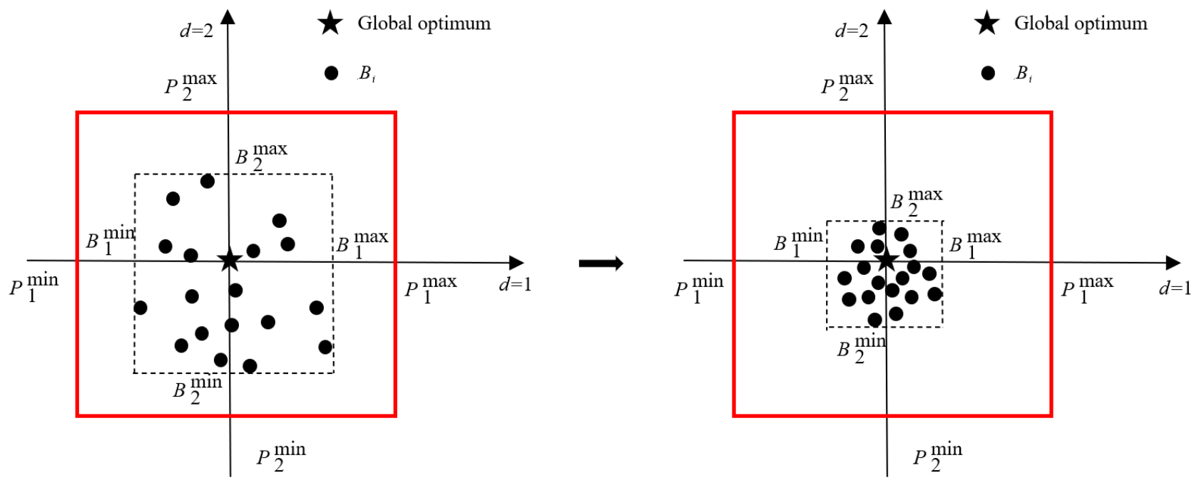
ECLPSO defines a dimensional normative interval [ B d min , B d max ] for each dimension d, where B d min and B d max are the smallest and largest personal best coordinates of all the particles on that dimension, respectively. This interval captures the effective search range of ECLPSO on each dimension. As optimization proceeds, the interval contracts steadily as the particles converge towards the global optimum, as illustrated in Figure 1.
To enhance the exploitation capacity of CLPSO, ECLPSO partitions the search on each dimension into an exploration phase and an exploitation phase based on the current width of the normative interval. Once the interval width satisfies the criterion in Equation (7), ECLPSO concludes the exploration phase on dimension d and enters the exploitation phase, updating Vi,d iteratively with Equation (8) instead of Equation (3).
B d max B d min α ( P d max P d min ) and B d max B d min β
V i , d = w pe V i , d + c pe r ( E i , d + η ( ( B d min + B d max ) / 2 E i , d ) P i , d )
where α = 0.01 is the relative threshold ratio; β = 2 is the absolute tolerance; and P d max and P d min are the upper and lower search bounds on dimension d. The dedicated inertia weight wpe = 0.5 and acceleration coefficient cpe = 1.5 are used exclusively during the perturbation-based exploitation. η ( ( B d min + B d max ) / 2 E i , d ) is the perturbation term. The perturbation magnitude η is sampled from a Gaussian distribution with mean 1 and standard deviation 0.65, and is clipped to within ten standard deviations on either side of the mean. The design of this perturbation is motivated by the observation of Yu and Zhang [13] that when the global optimum lies inside the normative interval it tends to reside near the interval’s center (i.e., ( B d min + B d max ) / 2 ). The perturbation term therefore grows with the distance between the particle’s position and the interval center—particles far from the center receive a larger correction, while those near the center receive a smaller one—driving thorough exploitation within the narrow normative interval. Note that Vi,d determined from Equation (8) is not subject to the dimensional maximum velocity constraint.
ECLPSO calculates the learning probability of each particle as a function of its personal best fitness rank and the number of dimensions currently in the exploitation phase, as given in Equation (9).
L i = L min + ( L max L min ) exp ( 10 ( T i 1 ) / ( N 1 ) ) 1 exp ( 10 ) 1
where Ti is the rank of particle i (Ti = 1 for the particle with the smallest personal best fitness); and Lmin and Lmax are the minimum and maximum learning probabilities, with Lmin = 0.05 (matching CLPSO) and Lmax updated adaptively using the equation given below.
L max = L min + 0.25 + 0.45 log ( D + 1 ) M k + 1
where Mk denotes the number of dimensions that have entered the exploitation phase by iteration k. As exploitation advances, Lmax grows logarithmically: the greater the number of dimensions in the exploitation phase, the larger Lmax becomes, steering the particles towards convergence.

3.3. Adaptive Comprehensive Learning Particle Swarm Optimization

Unlike CLPSO and ECLPSO which apply a unified maximum velocity and a single learning probability across all the dimensions, ACLPSO adapts the maximum velocity, inertia weight, acceleration coefficient and learning probability independently on each dimension based on the width of the corresponding normative interval. Each dimension d is assigned an independent inertia weight wd, acceleration coefficient cd, and per-particle learning probability Li,d. This dimension-wise adaptation enables particles to search each dimension at an appropriate granularity and achieves a natural balance between exploration and exploitation.
Specifically, ACLPSO adjusts the dimensional maximum velocity according to Equation (11).
V d max = s ( B d max B d min )
where s is the interval scaling coefficient mediating the influence of the normative interval width on the maximum velocity. When normative intervals are wide in the early phase, the large maximum velocity promotes coarse-grained exploration of broad search regions. As the algorithm matures, shrinking intervals reduce the maximum velocity, enabling finer-grained search and stronger exploitation.
When the condition in Equation (7) is not satisfied, the dimensional inertia weight wd is updated according to Equation (12).
w d = u B d max B d min P d max P d min + ( 1 u ) ( w max k K ( w max w min ) )
where u = 0.3 is a coefficient that balances the contributions of the normative interval width and the iteration counter. The value of wd is clipped to [wmin, wmax]: if wd < wmin, it is set to wmin; else if wd > wmax, it is set to wmax. To ensure particle convergence, wd and cd must jointly satisfy the following stability condition [14,34,35] derived from the theory of stochastic difference equations.
1 w d 0 and w d + 1 r c d   0
The key assumptions underlying the stability condition are: the exemplars are treated as fixed attractors over a short window of iterations; the random coefficients are drawn uniformly i.i.d. from [0, 1]; and the convergence is assessed in the mean squared sense. Accordingly, ACLPSO sets cd as:
c d = w d + 1
ACLPSO assigns a per-dimension learning probability Li,d to each particle according to Equation (15).
L i , d = v log K K + B d max B d min P d max P d min exp ( D ( T i 1 ) / ( N 1 ) ) 1 exp ( D ) 1
where the term vlogkK acts as a learning probability tradeoff that prevents Li,d from falling excessively low when a dimension enters the exploitation phase and its normative interval becomes very narrow. The coefficient v governs the maximum contribution of this stabilizing term. Like wd, Li,d is clipped to [Lmin, Lmax] with Lmin = 0.05 and Lmax = 0.75.
Different from CLPSO and ECLPSO, ACLPSO repairs the position of any particle that flies outside the search space and evaluates its fitness. The repairment is done by randomly reinitializing the position on a dimension between the previous feasible position and the trespassed bound.

4. Sigmoid Comprehensive Learning Particle Swarm Optimization

The dimensional maximum velocity and the per-dimension learning probability are the primary factors shaping ACLPSO’s convergence. As seen in Equations (11) and (15), these quantities are governed by the interval scaling coefficient s and the probability tradeoff coefficient v, respectively, making ACLPSO’s convergence sensitive to the chosen values of these two parameters. ACLPSO prescribes two candidate values for s (0.1 and 1.1) and two for v (0.05 and 0.3), yielding four possible value pairs. Experiments in [14] reveal that the optimal pair varies across benchmark functions, yet no decision rule is provided for selecting the best pair for a given problem. Practitioners must therefore try all the four pairs exhaustively, a process that is both inconvenient and computationally costly. To address this limitation, this paper replaces static assignment with iteration adaptive rules that continuously update s and v throughout the search.

4.1. Sigmoid Interval Scaling Coefficient

In Equation (11), s controls how strongly the normative interval width influences the maximum velocity. A smaller s attenuates this influence, yielding a weaker response to interval changes, whereas a larger s amplifies it. Choosing a suitable time-varying profile for s therefore requires understanding both how the maximum velocity affects convergence and how the normative interval evolves across iterations.
The maximum velocity primarily governs search granularity: a small maximum velocity enforces fine-grained search suitable for precise local refinement, while a large maximum velocity enables coarser exploration appropriate for broadly scanning large search regions. CLPSO and ECLPSO fix the maximum velocity on each dimension at 20% of the corresponding search bound, which can produce excessively coarse granularity in later iterations and consequently weak exploitation. Although ECLPSO partially compensates via its perturbation-based exploitation mechanism, it does not explicitly account for search granularity. Achieving a sound exploration exploitation balance therefore calls for a strategy that progressively reduces the maximum velocity as iterations advance. ACLPSO satisfies this requirement by coupling maximum velocity to the width of each dimension’s normative interval; as the interval contracts, the maximum velocity decreases accordingly, strengthening later phase exploitation.
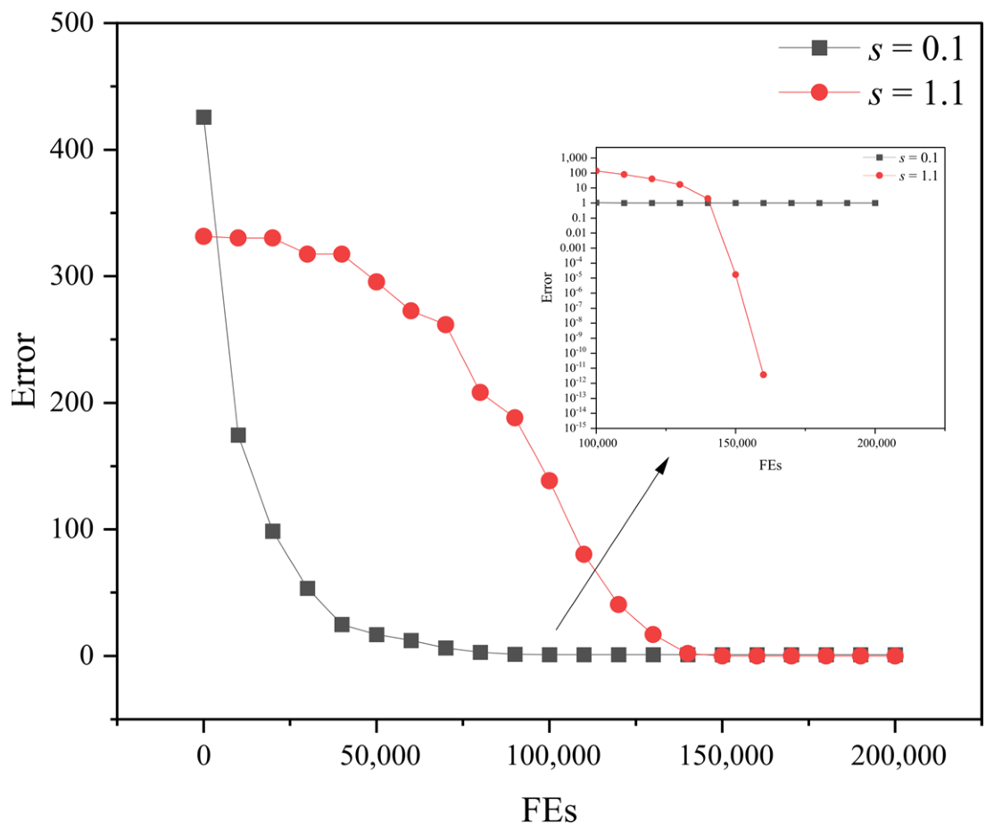
What effect does s exert on ACLPSO’s convergence? Empirical observations indicate that smaller values of s in the early iterations accelerate convergence. After a number of iterations—particularly when the exploitation phase begins—the normative interval width drops sharply, pulling the maximum velocity down with it. If s remains small at this point, the maximum velocity may become so restrictive that the particles struggle to fly towards better positions, as illustrated in Figure 2. To prevent this bottleneck, the value of s should be increased after a sufficient number of iterations, ensuring that the maximum velocity does not impede overall progress.
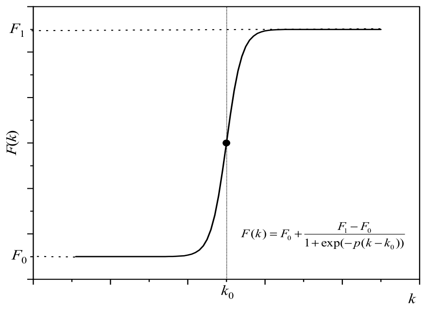
Based on these observations, a suitable schedule for s must maintain a small value in the early iterations and then transition rapidly to a larger value at a prescribed point, mitigating the adverse effect of the sharply contracting normative interval on the maximum velocity. The sigmoid function satisfies both requirements and is therefore adopted as the growth curve for s. The function and representative curves are shown in Figure 3, where k = k0 denotes the inflection point of maximum growth rate. Near this point, the curve ascends steeply from an initial level F0 to a final level F1. The parameter p controls the steepness of the transition: larger p produces a sharper rise near k0, while smaller p yields a more gradual increase.
The specific update equation for s is:
s = s 0 + s 1 s 0 1 + exp ( p s ( k k s ) )
where s0 = 0.1 and s1 = 1.1 are the initial (small) and final (large) target values of s, respectively. The rate parameter ps = 0.01 and the inflection point ks = K/5 were selected through systematic experimentation.

4.2. Sigmoid Probability Tradeoff Coefficient

The learning probability of a particle determines whether it favors its own personal best position (individual learning) or the personal best positions of other particles (social learning): a lower probability promotes individual learning, while a higher probability encourages social learning. ACLPSO assigns a separate learning probability to each dimension of every particle, so a single particle may simultaneously engage in individual learning on some dimensions and social learning on others. Dimensions that have not yet entered the exploitation phase retain relatively wide normative intervals, which map to higher learning probabilities that support continued exploration. Dimensions already in the exploitation phase have narrow intervals, producing lower learning probabilities that favor convergence. In Equation (15), the coefficient v caps the contribution of the tradeoff term. ACLPSO fixes v at one of two predefined values: 0.05 or 0.3.
The tradeoff term in Equation (15) prevents Li,d from shrinking excessively when a dimension’s normative interval becomes very narrow. v limits the maximum value of this stabilizing term. When v = 0.05, the cap falls at or below Lmin, driving all the dimensional learning probabilities to or below the minimum threshold. This effectively eliminates social learning and makes the particles highly vulnerable to local optima on complex multimodal problems. Conversely, a larger v causes the logarithmic tradeoff term to grow quickly in early iterations, keeping learning probabilities elevated and potentially hindering convergence in the early and later phases. The ideal behavior is therefore temporally adaptive: learning probabilities should remain relatively low initially to promote convergence, then rise in later iterations to maintain exploratory diversity and avoid premature stagnation.
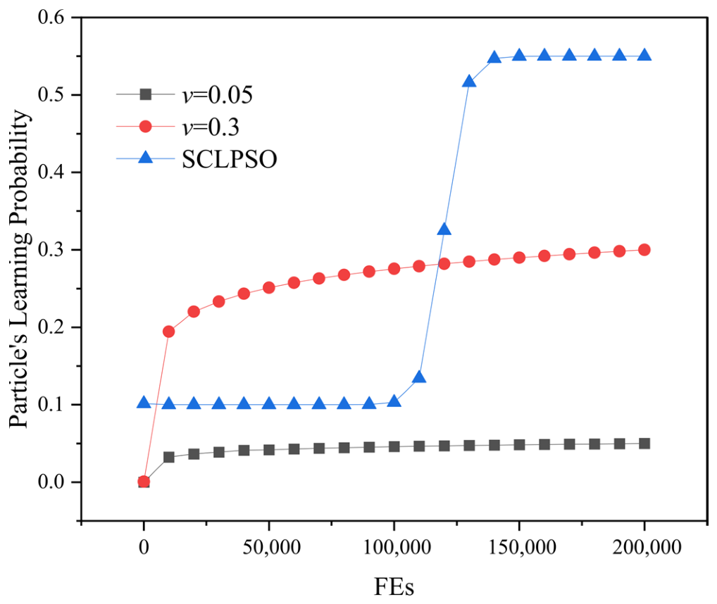
Based on this analysis, SCLPSO derives the learning probabilities according to a sigmoid schedule, as illustrated in Figure 4. In early iterations, the relatively low tradeoff value fosters convergence. As the search transitions to the later phase, the tradeoff value rises, enriching social learning and reducing the risk of premature stagnation at local optima. The per-dimension learning probability update equation for SCLPSO is:
v = v 0 + v 1 v 0 1 + exp ( p v ( k k v ) )
L i , d = v + B d max B d min P d max P d min   exp ( D ( T i 1 ) / ( N 1 ) ) 1 exp ( D ) 1
The key modification relative to ACLPSO is that the fixed probability tradeoff coefficient v is replaced by a sigmoid-driven term that transitions from v0 = 0.1 to v1 = 0.55. Compared with any fixed setting of v in ACLPSO, this change raises the learning probabilities in later iterations. The parameters pv = 0.01 and kv = 3K/5 were determined through systematic experimentation. The sigmoid tradeoff enables SCLPSO to deliver fast early convergence alongside strong later phase exploration, making it robust across a broad range of problem types.

4.3. Flowchart and Time Complexity

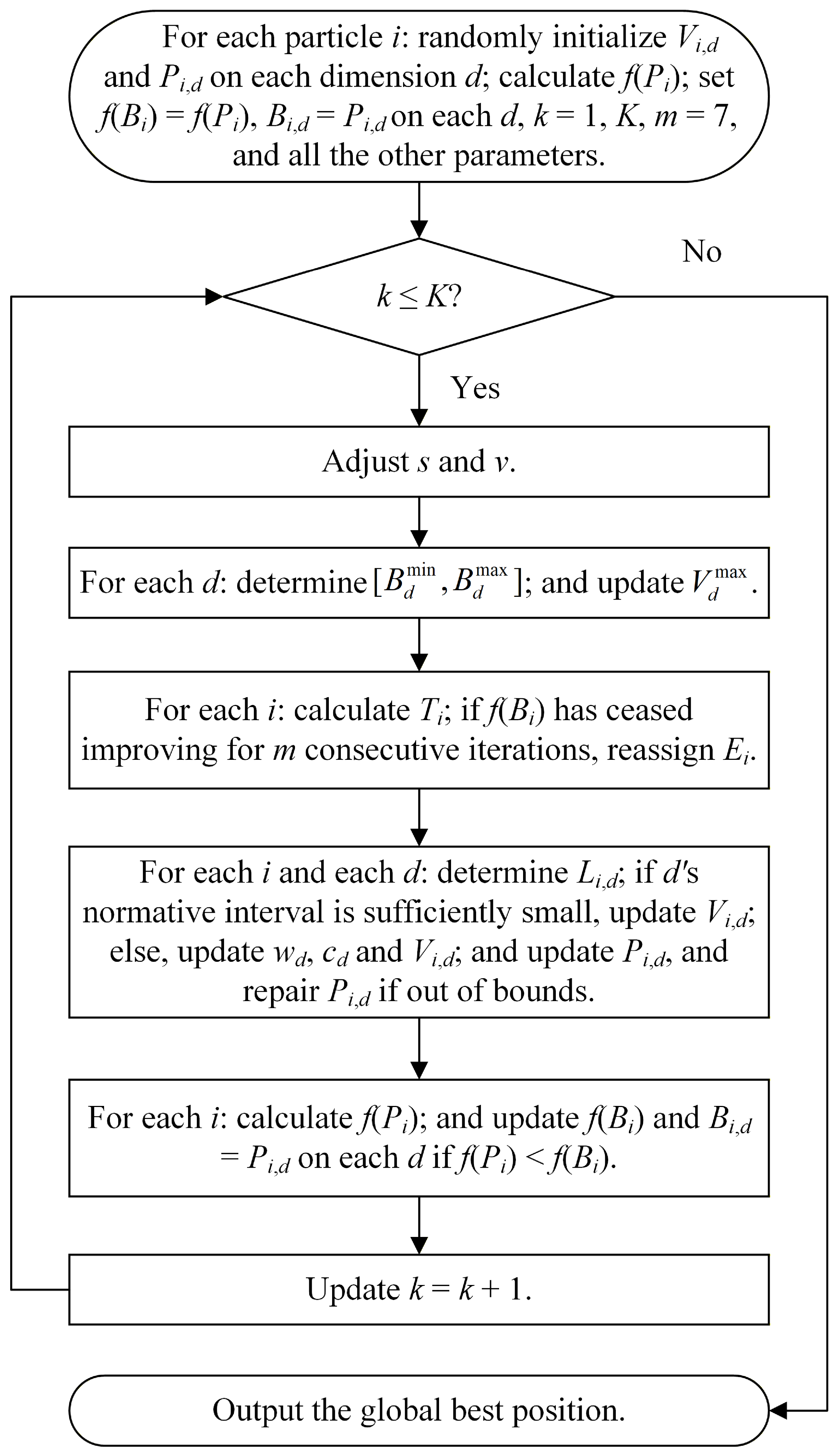
Figure 5 draws the flowchart of SCLPSO. In Figure 5, f denotes the fitness function. It can be seen that dynamically adjusting the interval scaling coefficient s according to Equation (16) and the probability tradeoff coefficient v following Equation (17) incurs additional computation burden as compared with ACLPSO, and the time complexity consumed by updating s and v is O(K) basic operations. However, the overall time complexity of SCLPSO is still O(K(NlogN + ND)) basic operations together with O(KN) function evaluations (FEs), the same as that of ACLPSO.

5. Experimental Results

This section answers the following questions through thorough experiments: (1) can SCLPSO locate the global optimum or a near-optimal solution on the majority of benchmark functions, and does it outperform ACLPSO configured with any fixed value pair of s and v? (2) what are the most appropriate parameter values for the sigmoid schedules in SCLPSO? and (3) does SCLPSO offer competitive advantages over other well-established PSO variants?
ACLPSO is instantiated as four variants with distinct parameter pairs: ACLPSO-1 (s = 0.1, v = 0.05), ACLPSO-2 (s = 1.1, v = 0.05), ACLPSO-3 (s = 0.1, v = 0.3), and ACLPSO-4 (s = 1.1, v = 0.3). Beyond these four ACLPSO variants, SCLPSO is also benchmarked against other prominent PSO variants, including CLPSO, ECLPSO, PSO-LDIW, PSO-CF, HPSO-TVAC and DNLPSO. The parameter settings for all the compared algorithms are listed in Table 1.

5.1. Benchmark Functions and Experimental Setup

This paper evaluates the search performance of SCLPSO and the compared PSO variants using sixteen classical benchmark functions [12,36,37]. These functions are grouped into five categories: unimodal, multimodal, shifted, rotated and shifted rotated. Table 2 lists their names, expressions, global optima, search spaces and categories. The number of dimensions D is set as 30, the swarm size N as 40, the maximum number of FEs as 200,000, and the maximum number of iterations K as 5000. Each algorithm is run independently 25 times on each function, and both the mean and standard deviation (SD) results of the solution error—the absolute difference between the obtained fitness value and the known global optimum—are recorded. To examine the generalization capability of SCLPSO further, all the PSO variants are additionally evaluated on the CEC2013 multimodal test suite. The CEC2013 suite comprises twenty benchmark functions: the first ten are basic multimodal functions defined in one to three dimensions; despite their low dimensionalities, their search spaces contain dense local optima. The remaining ten are composite functions constructed by combining multiple basic functions, producing highly irregular multimodal search landscapes. The full function definitions and composite construction details can be found in [15]. Table 3 lists the function names, dimensionality D, maximum FEs, global optima and swarm size N. The FE budgets and swarm sizes are assigned according to each function’s dimensionality and complexity.

5.2. Experimental Results and Analysis

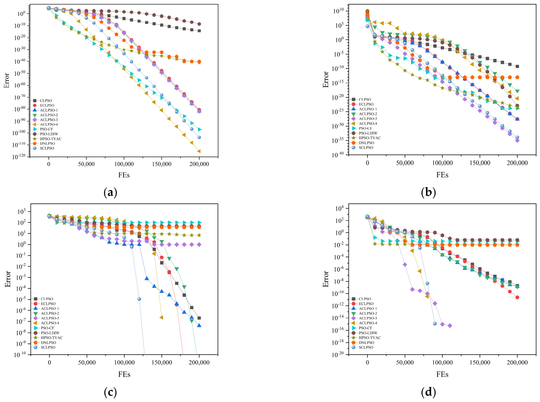
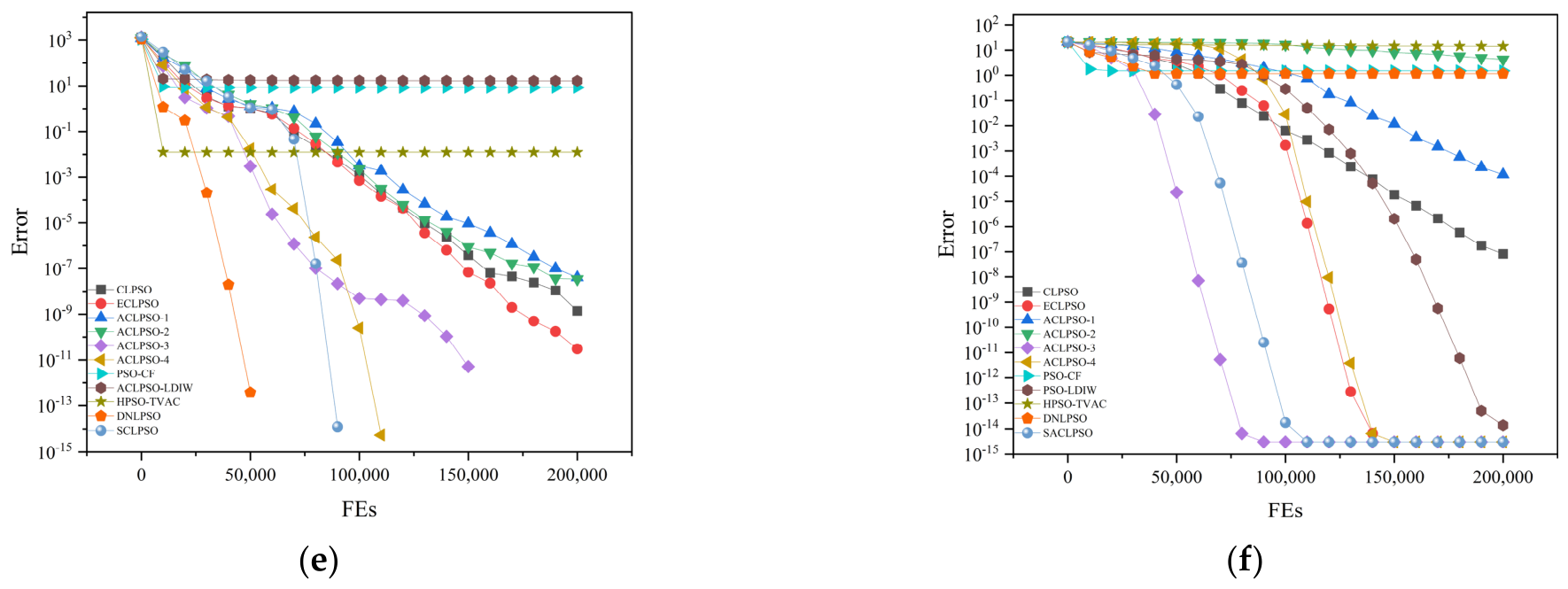
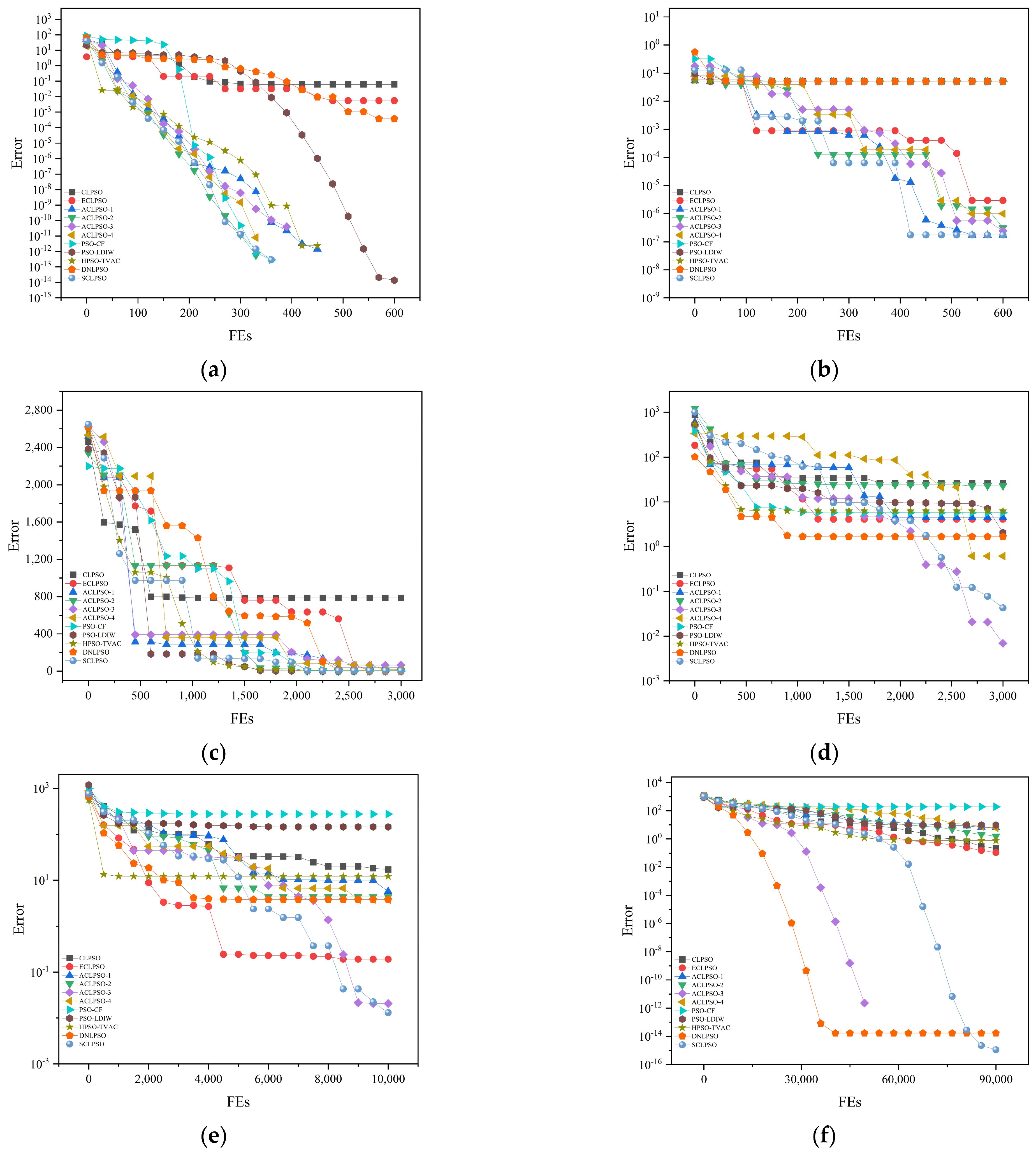
Table 4 reports the mean and SD errors over 25 independent runs for all the PSO variants on the sixteen classical benchmark functions, together with the per-function rankings (rank 1 = the smallest error relative to the global optimum). Figure 6 displays the convergence curves on representative functions f1, f2, f5, f8, f11 and f16, illustrating differences in terms of convergence speed and accuracy across algorithms. To assess statistical significance, the Wilcoxon signed rank test with the significance level at 0.05 is applied to compare SCLPSO with the four ACLPSO variants; the p-values and z-values are given in Table 5. A p-value below 0.05 indicates a significant performance difference, and the sign of the z-value determines direction: a negative z-value means that SCLPSO significantly surpasses the corresponding ACLPSO variant, while a positive z-value indicates the reverse. Table 6 and Table 7 examine the sensitivity of SCLPSO with respect to different values of ks/ps and kv/pv, respectively. Table 8 presents the analogous mean and SD errors and as well as the rankings on the CEC2013 multimodal test suite. The associated Wilcoxon test results are listed in Table 9. Figure 7 provides the convergence curves on selective CEC2013 functions.

5.2.1. Comparison of the Sixteen Classical Benchmark Functions

As shown in Table 4, no single ACLPSO variants achieves successfully finding the global optimum or a near-optimal solution on all the sixteen classical benchmark functions. Specifically, ACLPSO-1 attains a near-optimal solution only on f3; ACLPSO-2 reaches global or near-optimal on f5, f9 and f10; ACLPSO-3 is near-optimal on f1, f2, f4, f12 and f16; and ACLPSO-4 succeeds on f6, f7, f8, f11, f13, f14 and f15. A comparison of the four ACLPSO variants shows that ACLPSO-3 and ACLPSO-4 clearly outperform ACLPSO-1 and ACLPSO-2 by succeeding on a larger subset of functions. Both ACLPSO-3 and ACLPSO-4 use v = 0.3, reinforcing the observation that excessively small v values are detrimental to convergence—a key motivation for raising the upper bound of the tradeoff term in SCLPSO. SCLPSO achieves errors of the same order of magnitude as the best ACLPSO variant on f1, f2, f3, f5 to f12, and f16, and substantially outperforms the remaining three ACLPSO variants on f2, f4, f5, f6, f8, f9 and f11. These observations highlight SCLPSO’s primary advantage: it matches or approaches the accuracy of the best ACLPSO variant on most functions without requiring any manual coefficient tuning.
According to Table 4, on unimodal functions, SCLPSO is competitive, ranking below the best tuned ACLPSO variant on f1 to f3 and below HPSO-TVAC on f4, while excelling with top rankings on the multimodal functions f5 to f9. The ranking performance of SCLPSO on the shifted functions is mixed: SCLPSO leads on f11, but achieves only median rankings on f10 and f12. On the shifted rotated function f16, SCLPSO ranks the first. Though SCLPSO does not top on every individual function, its average rank across all the sixteen functions is 3.375 and is the lowest, placing it first among all the PSO variants in aggregate and confirming strong generalization capability in front of diverse problem types.
The Wilcoxon test results in Table 5 confirm that SCLPSO significantly beats three of the four ACLPSO variants (excluding the best tuned one) on f2, f4, f5, f6, f9, f11, f12 and f15. Moreover, SCLPSO demonstrates statistically significant superiority over at least one or two ACLPSO variants on all the remaining functions, with the exceptions of f13 and f14. Overall, SCLPSO consistently outperforms any single ACLPSO variant across the majority of benchmark functions.
The convergence curves in Figure 6 provide additional insight into per-function behavior. On the unimodal functions f1 and f2, all the algorithms avoid local optima traps, and differences appear primarily in exploitation accuracy. CLPSO converges to relatively poor solutions on both functions, indicating weak exploitation; by contrast, SCLPSO derives high accuracy solutions that exceed most competitors. On the multimodal functions f5, f8, f11 and f16, several PSO variants stagnate at local optima, while SCLPSO’s strong exploration capability prevents premature convergence. In summary, SCLPSO achieves rapid early phase convergence and high later phase accuracy, avoids local optima traps, and maintains a well calibrated exploration exploitation balance, thus overcoming the manual parameter tuning limitation of ACLPSO.

5.2.2. Determination of Relevant Parameters in SCLPSO

To identify the most suitable parameter values for the sigmoid schedules in SCLPSO, two sequential rounds of experiments are conducted. In the first round, the parameters ks and ps of the s update equation are determined. In the second round, using ks and ps fixed from round one, the parameters kv and pv of the v update equation are determined.
This paper evaluates SCLPSO across different combinations of ks and ps on the sixteen classical benchmark functions. Because the learning probability parameters had not yet been determined, the best static v value for each function—taken from the best performing ACLPSO variant on that function—was substituted. The parameter ks governs when s begins to grow, while ps controls the maximum growth rate. The results reported in Table 6 indicate that initiating growth around K/5 yields better convergence, and ps = 0.01 delivers the most consistent performance. Accordingly, ks = K/5 and ps = 0.01 are adopted.
Using the fixed values of ks and ps established in round one, multiple combinations of kv and pv are evaluated across the sixteen functions. According to Table 7, while several combinations of kv and pv allow SCLPSO to reach the global optimum or a near-optimal solution on f9 and f11, setting kv = 3K/5 and pv = 0.01 yields the best results on the greatest number of functions. These values are therefore adopted, enabling SCLPSO to solve the majority of functions successfully.

5.2.3. Comparison on the CEC2013 Multimodal Test Suite

To further assess the generalization performance of SCLPSO beyond classical benchmark functions, all the algorithms are additionally evaluated on the CEC2013 multimodal test suite. As shown in Table 7, on the first ten basic multimodal functions, SCLPSO achieves lower mean errors than all the four ACLPSO variants on f1, f3 and f4, and only marginally trails the best ACLPSO variant on f6 and f9. On the remaining functions—f2, f5, f7, f8 and f10—SCLPSO achieves results comparable to or within the same order of magnitude as the best ACLPSO variant. On the subsequent ten complex composite functions, SCLPSO performs strongly, with mean errors lower than all the four ACLPSO variants on most functions. SCLPSO ranks below the best ACLPSO variant only on f17, f18 and f19. Taken together, the results confirm that SCLPSO achieves superior overall performance over ACLPSO on the CEC2013 multimodal test suite, validating the effectiveness of the proposed improvements.
From the per-function rankings in Table 8, SCLPSO places first on f1 and f3, and remains competitively ranked on the remaining functions relative to other PSO variants. Its aggregate rank on the CEC2013 multimodal test suite is the third, surpassing all the four ACLPSO variants but falling behind DNLPSO and HPSO-TVAC. Compared with the rankings on the sixteen classical benchmark functions, SCLPSO’s standing has modestly declined. The modest decline warrants explanation. DNLPSO and HPSO-TVAC both retain direct learning from the global best position G, enabling them to converge rapidly on low-dimensional functions within a limited FEs budget. Among the twenty functions, f16 and f19 are 10-dimensional, f20 is 20-dimensional, and all the other functions are less than 5-dimensional. On f20, SCLPSO outperforms both DNLPSO and HPSO-TVAC, confirming its advantage on complex high-dimensional multimodal problems.
As can be seen from Table 9, for the low-dimensional functions f1 to f10 with relatively simple landscapes, SCLPSO exhibits no pronounced difference from the four ACLPSO variants, with the notable exceptions of f1, f2, f3, f5 and f6 on which SCLPSO significantly outperforms one or more ACLPSO variants. In contrast, for the more challenging composite functions f12, f13, f15, f16, f18 and f20, SCLPSO significantly conquers all the ACLPSO variants. Overall, SCLPSO holds a substantial convergence advantage over ACLPSO when addressing complex high-dimensional search spaces.
Figure 7 displays the convergence curves for selected CEC2013 functions. On the functions f1, f3 and f7, SCLPSO shows superior convergence: it achieves both faster early progress and closer approximation to the global optimum in the later iterations. On the composite functions, SCLPSO may not lead in the early phase, but it consistently converges to high accuracy solutions in the final iterations. Taken together, the results on both the classical and CEC2013 benchmark functions confirm that SCLPSO’s overall performance exceeds that of all the four ACLPSO variants, validating the effectiveness of the proposed algorithmic improvements.

6. Conclusions

This paper has proposed SCLPSO to eliminate the manual coefficient tuning required by ACLPSO. SCLPSO replaces the fixed value pairs of s and v in ACLPSO with sigmoid-based update rules that allow both coefficients to evolve continuously across iterations. It also reformulates the tradeoff term in the per-dimension learning probability update equation, treating the sigmoid-driven v as the sole tradeoff component. In addition, this paper has extended the empirical evaluation to the CEC2013 multimodal test suite beyond the sixteen classical benchmark functions used in prior work. Experimental results demonstrate that SCLPSO removes the need for manual parameter selection while achieving strong generalization: it identifies the global optimum or a near-optimal solution on the vast majority of benchmark functions, outperforms all the four ACLPSO variants configured with different (s, v) value pairs in terms of overall convergence, and surpasses most other PSO variants under comparison. However, SCLPSO is still somewhat limited in exploration as its convergence performance on some benchmark functions are still unsatisfactory.
The sigmoid function is a natural choice for updating s and v because of three strengths: (1) it is monotonically increasing and bounded within a prescribed range, ensuring that s and v remain within the desired operating intervals throughout the search; (2) it possesses an inflection point at which the rate of change is maximized, allowing precise control over the iteration at which the transition from exploration to exploitation is initiated; and (3) the single steepness provides an interpretable and independently controllable tradeoff between a gradual transition and an abrupt transition. Alternative adaptive schedules such as linear decay and cosine annealing lack the combination of strengths.
Future work will study further improvement to SCLPSO’s convergence on more challenging functions, comparison with more mainstream algorithms, and applications to practical engineering optimization problems including path planning and power system optimization, possibly learning from several recently proposed advanced swarm intelligence algorithms, e.g., gorilla troop optimization [39,40] and artificial protozoa optimization [41].

Author Contributions

Conceptualization, X.Y. and Y.Z.; methodology, Y.Z.; software, Y.Z.; validation, X.Y. and Y.Z.; formal analysis, Y.Z.; investigation, Y.Z.; resources, X.Y.; data curation, X.Y.; writing—original draft preparation, Y.Z.; writing—review and editing, X.Y.; visualization, Y.Z.; supervision, X.Y.; project administration, X.Y.; funding acquisition, X.Y. All authors have read and agreed to the published version of the manuscript.

Funding

This research was funded by the Jiangxi Province Natural Science Foundation, grant number 20224BAB204071 and the National Natural Science Foundation of China, grant number 52469002.

Data Availability Statement

The raw data supporting the conclusions of this article will be made available by the authors on request.

Conflicts of Interest

The authors declare no conflict of interest.

References

  1. Kennedy, J.; Eberhart, R. Particle swarm optimization. In Proceedings of the ICNN’95-International Conference on Neural Networks, Perth, WA, Australia, 27 November–1 December 1995. [Google Scholar]
  2. Ekrem, Ö.; Aksoy, B. Trajectory planning for a 6-axis robotic arm with particle swarm optimization algorithm. Eng. Appl. Artif. Intell. 2023, 122, 106099. [Google Scholar] [CrossRef]
  3. Tao, B.; Kim, J.-H. Mobile robot path planning based on bi-population particle swarm optimization with random perturbation strategy. J. King Saud Univ.—Comput. Inf. Sci. 2024, 36, 101974. [Google Scholar] [CrossRef]
  4. Huang, C.; Zhou, X.; Ran, X.; Wang, J.; Chen, H.; Deng, W. Adaptive cylinder vector particle swarm optimization with differential evolution for UAV path planning. Eng. Appl. Artif. Intell. 2023, 121, 105942. [Google Scholar] [CrossRef]
  5. Tiwari, S.; Kumar, A. Advances and bibliographic analysis of particle swarm optimization applications in electrical power system: Concepts and variants. Evol. Intell. 2023, 16, 23–47. [Google Scholar] [CrossRef]
  6. Di Cesare, N.; Domaszewski, M. A new hybrid topology optimization method based on I-PR-PSO and ESO. Application to continuum structural mechanics. Comput. Struct. 2019, 212, 311–326. [Google Scholar] [CrossRef]
  7. Eberhart, R.; Kennedy, J. A new optimizer using particle swarm theory. In Proceedings of the MHS’95. Proceedings of the Sixth International Symposium on Micro Machine and Human Science, Nagoya, Japan, 4–6 October 1995. [Google Scholar]
  8. Shi, Y.; Eberhart, R. A modified particle swarm optimizer. In Proceedings of the 1998 IEEE International Conference on Evolutionary Computation Proceedings. IEEE World Congress on Computational Intelligence (Cat. No. 98TH8360), Anchorage, AK, USA, 4–9 May 1998. [Google Scholar]
  9. Črepinšek, M.; Liu, S.-H.; Mernik, M. Exploration and exploitation in evolutionary algorithms: A survey. ACM Comput. Surv. 2013, 45, 1–33. [Google Scholar] [CrossRef]
  10. Liang, J.J.; Qin, A.K.; Suganthan, P.N.; Baskar, S. Comprehensive learning particle swarm optimizer for global optimization of multimodal functions. IEEE Trans. Evol. Comput. 2006, 10, 281–295. [Google Scholar] [CrossRef]
  11. Nasir, M.; Das, S.; Maity, D.; Sengupta, S.; Halder, U.; Suganthan, P. A dynamic neighborhood learning based particle swarm optimizer for global numerical optimization. Inf. Sci. 2012, 209, 16–36. [Google Scholar] [CrossRef]
  12. Zhan, Z.-H.; Zhang, J.; Liu, O. Orthogonal learning particle swarm optimization. In Proceedings of the 11th Annual Conference on Genetic and Evolutionary Computation, Montreal, QC, Canada, 8–12 July 2009. [Google Scholar]
  13. Yu, X.; Zhang, X. Enhanced comprehensive learning particle swarm optimization. Appl. Math. Comput. 2014, 242, 265–276. [Google Scholar] [CrossRef]
  14. Yu, X.; Qiao, Y. Enhanced Comprehensive Learning Particle Swarm Optimization with Dimensional Independent and Adaptive Parameters. Comput. Intell. Neurosci. 2021, 2021, 6628564. [Google Scholar] [CrossRef] [PubMed]
  15. Li, X.; Engelbrecht, A.; Epitropakis, M.G. Benchmark Functions for CEC’2013 Special Session and Competition on Niching Methods for Multimodal Function Optimization; Technical Report; RMIT University, Evolutionary Computation and Machine Learning Group: Melbourne, Australia, 2013. [Google Scholar]
  16. Shi, Y.; Eberhart, R.C. Parameter selection in particle swarm optimization. In International Conference on Evolutionary Programming; Springer: Berlin/Heidelberg, Germany, 1998. [Google Scholar]
  17. Shi, Y.; Eberhart, R.C. Empirical study of particle swarm optimization. In Proceedings of the 1999 Congress on Evolutionary Computation-CEC99 (Cat. No. 99TH8406), Washington, DC, USA, 6–9 July 1999. [Google Scholar]
  18. Shi, Y.; Eberhart, R.C. Fuzzy adaptive particle swarm optimization. In Proceedings of the 2001 Congress on Evolutionary Computation (IEEE Cat. No. 01TH8546), Seoul, Republic of Korea, 27–30 May 2001. [Google Scholar]
  19. Peram, T.; Veeramachaneni, K.; Mohan, C.K. Fitness-distance-ratio based particle swarm optimization. In Proceedings of the 2003 IEEE Swarm Intelligence Symposium. SIS’03 (Cat. No. 03EX706), Indianapolis, IN, USA, 26 April 2003. [Google Scholar]
  20. Ratnaweera, A.; Halgamuge, S.K.; Watson, H.C. Self-Organizing Hierarchical Particle Swarm Optimizer with Time-Varying Acceleration Coefficients. IEEE Trans. Evol. Comput. 2004, 8, 240–255. [Google Scholar] [CrossRef]
  21. Clerc, M.; Kennedy, J. The particle swarm-explosion, stability, and convergence in a multidimensional complex space. IEEE Trans. Evol. Comput. 2002, 6, 58–73. [Google Scholar] [CrossRef]
  22. Barrera, J.; Coello Coello, C.A. Limiting the velocity in particle swarm optimization using a geometric series. In Proceedings of the 11th Annual Conference on Genetic and Evolutionary Computation, Montreal, QC, Canada, 8–12 July 2009. [Google Scholar]
  23. Barrera, J.; Bajo, O.Á.; Flores, J.J.; Coello, C.A.C. Limiting the velocity in the particle swarm optimization algorithm. Comput. Sist. 2016, 20, 635–645. [Google Scholar] [CrossRef][Green Version]
  24. Li, X.; Mao, K.; Lin, F.; Zhang, X. Particle swarm optimization with state-based adaptive velocity limit strategy. Neurocomputing 2021, 447, 64–79. [Google Scholar] [CrossRef]
  25. Kennedy, J.; Mendes, R. Population structure and particle swarm performance. In Proceedings of the 2002 Congress on Evolutionary Computation. CEC’02 (Cat. No. 02TH8600), Honolulu, HI, USA, 12–17 May.
  26. Suganthan, P.N. Particle swarm optimiser with neighbourhood operator. In Proceedings of the 1999 Congress on Evolutionary Computation-CEC99 (Cat. No. 99TH8406), Washington, DC, USA, 6–9 July 1999. [Google Scholar]
  27. Mendes, R.; Kennedy, J.; Neves, J. The fully informed particle swarm: Simpler, maybe better. IEEE Trans. Evol. Comput. 2004, 8, 204–210. [Google Scholar] [CrossRef]
  28. Zeng, N.; Wang, Z.; Liu, W.; Zhang, H.; Hone, K.; Liu, X. A dynamic neighborhood-based switching particle swarm optimization algorithm. IEEE Trans. Cybern. 2020, 52, 9290–9301. [Google Scholar] [CrossRef] [PubMed]
  29. Chen, Y.; Peng, W.; Jian, M. Particle swarm optimization with recombination and dynamic linkage discovery. IEEE Trans. Syst. Man Cybern. Part B—Cybern. 2007, 37, 1460–1470. [Google Scholar] [CrossRef]
  30. Cao, Y.; Zhang, H.; Li, W.; Zhou, M.; Zhang, Y.; Chaovalitwongse, W.A. Comprehensive Learning Particle Swarm Optimization Algorithm with Local Search for Multimodal Functions. IEEE Trans. Evol. Comput. 2019, 23, 718–731. [Google Scholar] [CrossRef]
  31. Das, S.; Abraham, A.; Konar, A. Particle swarm optimization and differential evolution algorithms: Technical analysis, applications and hybridization perspectives. In Advances of Computational Intelligence in Industrial Systems; Springer: Berlin/Heidelberg, Germany, 2008; pp. 1–38. [Google Scholar]
  32. Şenel, F.A.; Gökçe, F.; Yüksel, A.S.; Yiğit, T. A novel hybrid PSO–GWO algorithm for optimization problems. Eng. Comput. 2019, 35, 1359–1373. [Google Scholar] [CrossRef]
  33. Pozna, C.; Precup, R.-E.; Horvath, E.; Petriu, E.M. Hybrid particle filter–particle swarm optimization algorithm and application to fuzzy controlled servo systems. IEEE Trans. Fuzzy Syst. 2022, 30, 4286–4297. [Google Scholar] [CrossRef]
  34. García-Gonzalo, E.; Fernández-Martínez, J.L. Convergence and stochastic stability analysis of particle swarm optimization variants with generic parameter distributions. Appl. Math. Comput. 2014, 249, 286–302. [Google Scholar] [CrossRef]
  35. Taherkhani, M.; Safabakhsh, R. A novel stability-based adaptive inertia weight for particle swarm optimization. Appl. Soft Comput. 2016, 38, 281–295. [Google Scholar] [CrossRef]
  36. Meng, A.; Li, Z.; Yin, H.; Chen, S.; Guo, Z. Accelerating particle swarm optimization using crisscross search. Inf. Sci. 2016, 329, 52–72. [Google Scholar] [CrossRef]
  37. Suganthan, P.N.; Hansen, N.; Liang, J.J.; Deb, K.; Tiwari, S. Problem definitions and evaluation criteria for the CEC 2005 special session on real-parameter optimization. KanGAL Rep. 2005, 341–357. [Google Scholar]
  38. Salomon, R. Re-evaluating genetic algorithm performance under coordinate rotation of benchmark functions. A survey of some theoretical and practical aspects of genetic algorithms. BioSystems 1996, 39, 263–278. [Google Scholar] [CrossRef] [PubMed]
  39. Abdollahzadeh, B.; Soleimanian Gharehchopogh, F.; Mirjalili, S. Artificial gorilla troops optimizer: A new nature-inspired metaheuristic algorithm for global optimization problems. Int. J. Intell. Syst. 2021, 36, 5887–5958. [Google Scholar] [CrossRef]
  40. You, J.; Jia, H.; Wu, D.; Rao, H.; Wen, C.; Liu, Q.; Abualigah, L. Modified artificial gorilla troop optimization algorithm for solving constrained engineering optimization problems. Mathematics 2023, 11, 1256. [Google Scholar] [CrossRef]
  41. Shehab, M. Artificial protozoa optimizer: A bio-inspired metaheuristic for complex engineering optimization. Results Eng. 2025, 27, 106883. [Google Scholar] [CrossRef]
Figure 1. Variation trend of the dimensional normative interval in a two-dimensional problem.
Mathematics 14 01854 g001
Figure 2. Optimization performance of ACLPSO with different s values on the 30-dimensional Rastrigin function.
Mathematics 14 01854 g002
Figure 3. Generalized sigmoid functions and curves of variation.
Mathematics 14 01854 g003
Figure 4. Variation in particle’s learning probability in ACLPSO and SCLPSO.
Mathematics 14 01854 g004
Figure 5. Flowchart of SCLPSO.
Mathematics 14 01854 g005
Figure 6. Convergence curves of all the algorithms on certain classical benchmark functions. (a) f1, (b) f2, (c) f5, (d) f8, (e) f11, (f) f16.
Mathematics 14 01854 g006aMathematics 14 01854 g006b
Figure 7. Convergence curves of all the algorithms on certain CEC2013 benchmark functions. (a) f1, (b) f3, (c) f7, (d) f17, (e) f18, (f) f20.
Mathematics 14 01854 g007
Table 1. Parameter settings of the PSO variants involved in comparison.
PSO VariantsParameters Settings
PSO-LDIW [17]c1 = c2 = 2.0, w = 0.9~0.4.
PSO-CF [21]χ = 0.729, c1 = c2 = 2.05.
HPSO-TVAC [20]c1 = 2.5~0.5, c2 = 0.5~2.5, w = 0.9~0.4
CLPSO [10]w = 0.9~0.4, m = 7, c = 1.49445.
DNLPSO [11]w = 0.9~0.4, m = 7, c1 = c2 = 1.49445, g = 10.
ECLPSO [13]w = 0.9~0.4, m = 7, c = 1.49445.
ACLPSO [14]m = 7, s = 0.1 or 1.1, v = 0.05 or 0.3.
SCLPSOm = 7
Table 2. Sixteen classical benchmark functions.
NameExpressionSearch Spacex*f(x*)Category
Sphere f 1 ( x ) = d = 1 D x d 2 100 ,   100 D 0 D 0Unimodal
Schwefel P2.22 f 2 ( x ) = d = 1 D x d + d = 1 D x d 10 ,   10 D 0 D 0
Rosenbrock f 3 ( x ) = d = 1 D 1 ( 100 ( x d + 1 x d 2 ) 2 + ( x d 1 ) 2 ) 10 ,   10 D 0 D 0
Schwefel P1.2 f 4 ( x ) = d = 1 D ( j = 1 d x j ) 2 100 ,   100 D 0 D 0
Rastrigin f 5 ( x ) = 10 D + d = 1 D ( x d 10 cos ( 2 π x d ) ) 5.12 ,   5.12 D 0 D 0Multimodal
Noncontinuous Rastrigin f 6 ( x ) = f 5 ( y ) , y d = x d , if x d < 0.5 , round ( 2 x d ) / 2 , otherwise 5.12 ,   5.12 D 0 D 0
Ackley f 7 ( x ) = 20 exp ( 0.2 ( 1 / D ) d = 1 D x d 2 ) exp ( ( 1 / D ) d = 1 D cos ( 2 π x d ) ) + 20 + e 32 ,   32 D 0 D 0
Griewank f 8 ( x ) = 1 / 4000 d = 1 D x d 2 d = 1 D cos ( x d / d ) + 1 600 ,   600 D 0 D 0
Schwefel f 9 ( x ) = 418.9828 D d = 1 D x d sin ( x d ) 500 ,   500 D 420.96 D 0
Shifted Rosenbrock f 10 ( x ) = f 3 ( y ) , y d = x d o d + 1 100 ,   100 D o 0Shifted
Shifted Griewank f 11 ( x ) = f 8 ( y ) , y d = x d o d 600 ,   600 D o 0
Shifted Schwefel P1.2 f 12 ( x ) = f 4 ( y ) , y d = x d o d 100 ,   100 D o 0
Rotated Rastrigin f 13 ( x ) = f 5 ( y ) , y d = x · M 5.12 ,   5.12 D 0 D 0Rotated
Rotated Schwefel f 14 ( x ) = f 9 ( y ) , y d = z d sin ( z d ) , if z d 500 , 0 , otherwise , z = { x d 420.96 } D · M + { 420.96 } D 500 ,   500 D 420.96 D 0
Rotated Griewank f 15 ( x ) = f 8 ( y ) , y d = x · M 600 ,   600 D 0 D 0
Shifted Rotated Ackley f 16 ( x ) = f 7 ( y ) , y d = ( x o ) · M 32 ,   32 D o 0Shifted Rotated
{}D denotes a D-dimensional vector, o is the shifted global optimum, M is a D-dimensional orthogonal matrix that is generated using Salomon’s methods [38].
Table 3. CEC2013 multimodal benchmark functions.
NameIndexDFEsNf(x*)Search Space
Five-Uneven-Peak Trapf1160012200.0 x 0 ,   30
Equal Maximaf21600121.0 x 0 ,   1
Uneven Decreasing Maximaf31600121.0 x 0 ,   1
Himmelblauf42120012200.0 x ,   y [ 6 ,   6 ]
Six-Hump Camel Backf521200121.03163 x 1.9 , 1.9
y 1.1 , 1.1
Shubertf62120012186.713 0.25 ,   10 D
f733000202709.0935
Vincentf821200121.0 [ 10 ,   10 ] D
f933000201.0
Modified Rastriginf1021200122.0 0 ,   1 D
Composition Function 1f1121500120 [ 5 ,   5 ] D
Composition Function 2f1221500120 [ 5 ,   5 ] D
Composition Function 3f1321500120 [ 5 ,   5 ] D
f1433000200
f15510,000200
f161030,000300
Composition Function 4f1733000200 [ 5 ,   5 ] D
f18510,000300
f191030,000300
f202090,000400
Table 4. Performance comparison of various algorithms on the sixteen classical benchmark functions.
FunctionMetricsACLPSO-1ACLPSO-2ACLPSO-3ACLPSO-4CLPSOECLPSODNLPSOHPSO-TVACPSO-CFPSO-LDIWSCLPSO
f1Mean2.87 × 10−121.23 × 10−103.28 × 10−1153.37 × 10−152.34 × 10−142.74 × 10−934.36 × 10−346.26 × 10−361.50 × 10−931.91 × 10−321.17 × 10⁻¹³
SD8.18 × 10−126.08 × 10−106.11 × 10−1159.36 × 10−153.77 × 10−144.71 × 10−931.91 × 10−331.12 × 10−356.00 × 10−934.13 × 10−323.78 × 10⁻¹³
Rank1011129576483
f2Mean3.09 × 10−291.48 × 10−177.25 × 10−374.74 × 10−226.55 × 10−102.34 × 10−272.71 × 10−125.86 × 10−211.30 × 10−238.00 × 10−13.51 × 10−35
SD4.27 × 10−292.19 × 10−176.84 × 10−379.70 × 10−226.64 × 10−102.29 × 10−271.29 × 10−119.96 × 10−215.76 × 10−232.77 × 1005.41 × 10−35
SD3816104975112
f3Mean1.84 × 1004.23 × 1002.61 × 1016.56 × 1013.98 × 1012.98 × 1011.75 × 1012.05 × 1011.44 × 1043.40 × 1011.03 × 101
SD1.63 × 1002.43 × 1002.87 × 1012.49 × 1011.90 × 1012.12 × 1012.16 × 1011.69 × 1013.37 × 1042.25 × 1012.33 × 101
Rank1261097451183
f4Mean3.39 × 1021.56 × 1047.87 × 10−21.71 × 1044.48 × 1025.57 × 1023.82 × 10−21.92 × 10−44.00 × 1022.00 × 1026.35 × 100
SD8.84 × 1013.44 × 1038.72 × 10−28.24 × 1031.01 × 1021.37 × 1021.14 × 10−11.81 × 10−41.38 × 1031.00 × 1033.49 × 100
Rank6103118921754
f5Mean5.17 × 10−10.00 × 1003.02 × 1001.55 × 1001.76 × 10−60.00 × 1003.08 × 1017.40 × 1009.57 × 1016.50 × 1010.00 × 100
SD5.83 × 10−10.00 × 1001.45 × 1009.12 × 10−11.94 × 10−60.00 × 1006.59 × 1002.96 × 1002.50 × 1011.90 × 1010.00 × 100
Rank5176419811101
f6Mean5.66 × 10−14.19 × 10−12.00 × 10−10.00 × 1000.00 × 1004.60 × 10−33.76 × 1002.80 × 10−16.72 × 1003.20 × 10−10.00 × 100
SD6.63 × 10−17.19 × 10−14.08 × 10−10.00 × 1000.00 × 1002.19 × 10−21.79 × 1006.78 × 10−12.67 × 1005.57 × 10−10.00 × 100
Rank9851141061171
f7Mean1.15 × 10−81.92 × 10−63.25 × 10−153.11 × 10−153.88 × 10−83.11 × 10−151.27 × 10−139.79 × 10−141.22 × 1001.16 × 10−143.11 × 10⁻¹⁵
SD5.77 × 10−86.96 × 10−67.11 × 10−160.00 × 1002.72 × 10−80.00 × 1001.86 × 10−133.59 × 10−141.11 × 1003.70 × 10−150.00 × 100
Rank8104191761151
f8Mean1.87 × 10−83.35 × 10−81.38 × 10−110.00 × 1001.34 × 10−91.43 × 10−107.98 × 10−37.78 × 10−33.19 × 10−21.57 × 10−20.00 × 100
SD3.45 × 10−83.88 × 10−84.56 × 10−110.00 × 1002.74 × 10−93.28 × 10−101.16 × 10−21.00 × 10−28.34 × 10−21.68 × 10−20.00 × 100
Rank6731549811101
f9Mean2.23 × 1023.82 × 10−45.87 × 1024.29 × 1023.82 × 10−43.82 × 10−41.88 × 1031.63 × 1035.85 × 1035.13 × 1033.82 × 10−4
SD1.38 × 1029.15 × 10−72.04 × 1022.71 × 1024.90 × 10−133.94 × 10−113.11 × 1023.35 × 1026.88 × 1027.18 × 1020.00 × 100
Rank5476239811101
f10Mean2.62 × 1011.67 × 1019.18 × 1018.54 × 1022.89 × 1019.85 × 1013.51 × 1017.07 × 1013.51 × 1075.50 × 1071.21 × 102
SD2.01 × 1011.46 × 1019.29 × 1012.45 × 1031.74 × 1013.36 × 1015.08 × 1018.25 × 1019.40 × 1079.79 × 1074.41 × 101
Rank2169374510118
f11Mean1.28 × 10−71.26 × 10−71.96 × 10−30.00 × 1008.16 × 10−108.32 × 10−109.06 × 10−32.03 × 10−21.24 × 1012.04 × 1010.00 × 100
SD2.34 × 10−73.30 × 10−78.01 × 10−30.00 × 1001.11 × 10−92.21 × 10−91.10 × 10−21.96 × 10−29.35 × 1001.28 × 1010.00 × 100
Rank6571348910111
f12Mean1.33 × 1037.40 × 1032.60 × 1001.50 × 1031.35 × 1031.65 × 1031.27 × 10−25.89 × 10−47.91 × 1001.83 × 1016.74 × 101
SD3.07 × 1021.77 × 1031.71 × 1007.37 × 1023.49 × 1022.48 × 1022.33 × 10−26.18 × 10−43.01 × 1014.45 × 1015.05 × 101
Rank7113981021456
f13Mean2.04 × 1013.65 × 1011.39 × 1013.25 × 1002.59 × 1012.04 × 1015.56 × 1012.59 × 1018.53 × 1016.65 × 1017.03 × 101
SD3.70 × 1007.40 × 1002.53 × 1001.88 × 1004.60 × 1003.70 × 1001.62 × 1019.40 × 1001.71 × 1011.88 × 1017.50 × 100
Rank3721548611910
f14Mean1.35 × 1035.78 × 1021.32 × 1032.53 × 1021.25 × 1031.23 × 1032.29 × 1032.08 × 1035.88 × 1035.15 × 1034.37 × 103
SD1.85 × 1024.00 × 1022.19 × 1022.09 × 1021.19 × 1021.42 × 1022.98 × 1027.10 × 1027.82 × 1026.50 × 1022.58 × 102
Rank6251438711109
f15Mean1.65 × 10−32.05 × 10−32.76 × 10−35.33 × 10−171.10 × 10−44.51 × 10−31.32 × 10−21.11 × 10−22.97 × 10−21.52 × 10−22.41 × 10⁻⁸
SD2.70 × 10−32.71 × 10−35.91 × 10−36.51 × 10−173.01 × 10−43.10 × 10−31.61 × 10−21.23 × 10−22.77 × 10−21.51 × 10−21.16 × 10⁻⁷
Rank4561379811102
f16Mean1.74 × 10−62.73 × 10−53.82 × 10−153.96 × 10−154.13 × 10−73.96 × 10−154.21 × 10−12.82 × 1001.94 × 1001.29 × 10−143.82 × 10⁻¹⁵
SD6.94 × 10−69.24 × 10−51.45 × 10−151.55 × 10−156.94 × 10−61.55 × 10−156.42 × 10−14.65 × 1001.53 × 1003.12 × 10−151.45 × 10⁻¹⁵
Rank7823649111051
Average Rank5.56.254.254.31255.56254.81257.1256.3759.31258.43753.375
Final Rank5723649811101
Table 5. Wilcoxon signed rank test results of SCLPSO against the four ACLPSO variants on the sixteen classical benchmark functions.
FunctionACLPSO-1ACLPSO-2ACLPSO-3ACLPSO-4
p-Valuez-Valuep-Valuez-Valuep-Valuez-Valuep-Valuez-Value
f15.960 × 10−8−4.359 × 1005.960 × 10−8−4.363 × 1004.172 × 10−64.036 × 1006.670 × 10−21.830 × 100
f25.960 × 10−8−4.359 × 1005.960 × 10−8−4.359 × 1005.960 × 10−84.359 × 1005.960 × 10−8−4.359 × 100
f38.081 × 10−43.175 × 1002.027 × 10−22.287 × 1007.915 × 10−1−2.691 × 10−11.150 × 10−3−3.094 × 100
f45.960 × 10−8−4.359 × 1005.960 × 10−8−4.359 × 1005.960 × 10−84.359 × 1005.960 × 10−8−4.359 × 100
f56.104 × 10−5−3.379 × 1001.000 × 1000.000 × 1001.192 × 10−7−4.307 × 1005.960 × 10−8−4.359 × 100
f62.441 × 10−4−3.145 × 1003.052 × 10−5−3.490 × 1002.441 × 10−4−3.145 × 1001.000 × 1000.000 × 100
f73.125 × 10−2−2.102 × 1001.950 × 10−3−2.752 × 1005.000 × 10−1−8.944 × 10−11.000 × 1000.000 × 100
f81.250 × 10−1−1.643 × 1005.960 × 10−8−4.359 × 1001.250 × 10−1−1.643 × 1001.000 × 1000.000 × 100
f95.960 × 10−8−4.359 × 1001.000 × 1000.000 × 1005.960 × 10−8−4.361 × 1001.907 × 10−6−3.905 × 100
f102.980 × 10−74.278 × 1002.980 × 10−74.278 × 1004.908 × 10−16.996 × 10−16.915 × 10−14.036 × 10⁻¹
f115.960 × 10−8−4.359 × 1005.960 × 10−8−4.359 × 1003.910 × 10−3−2.606 × 1001.000 × 1000.000 × 100
f125.960 × 10−8−4.359 × 1005.960 × 10−8−4.359 × 1005.960 × 10−84.359 × 1005.960 × 10−8−4.359 × 100
f135.960 × 10−84.359 × 1002.980 × 10−74.278 × 1005.960 × 10−84.359 × 1005.960 × 10−84.359 × 100
f145.960 × 10−84.359 × 1005.960 × 10−84.359 × 1005.960 × 10−84.359 × 1005.960 × 10−84.359 × 100
f154.542 × 10−5−3.713 × 1005.388 × 10−5−3.686 × 1008.796 × 10−11.465 × 10−17.600 × 10−32.577 × 100
f169.766 × 10−4−2.942 × 1005.960 × 10−8−4.359 × 1007.539 × 10−1−5.750 × 10−12.891 × 10−1−1.336 × 100
Table 6. Comparison of the mean errors of SCLPSO on different functions for different ks and ps.
FunctionMetricsps = 0.1ps = 0.05ps = 0.01ps = 0.005ps = 0.001
f2
(v = 0.3)
ks = K/59.62 × 10−378.63 × 10−375.40 × 10−376.58 × 10−379.11 × 10⁻²⁵
ks = 2K/51.57 × 10−237.47 × 10−376.87 × 10−371.38 × 10−366.01 × 10⁻³⁵
ks = 3K/51.44 × 10−361.47 × 10−361.37 × 10−369.34 × 10−372.27 × 10−36
ks = 4K/58.86 × 10−371.48 × 10−361.11 × 10−361.14 × 10−369.96 × 10−37
f4
(v = 0.3)
ks = K/55.39 × 10−16.17 × 10−18.14 × 10−13.80 × 1011.38 × 104
ks = 2K/51.51 × 10−11.41 × 10−12.43 × 10−12.18 × 10−11.60 × 10³
ks = 3K/56.62 × 10−21.05 × 10−17.46 × 10−23.12 × 10−11.03 × 101
ks = 4K/53.66 × 10−19.70 × 10−21.02 × 1006.69 × 10−22.11 × 10⁻¹
f5
(v = 0.05)
ks = K/51.16 × 10−55.88 × 10−64.79 × 10−71.53 × 10−56.20 × 10⁻⁶
ks = 2K/51.12 × 10−41.63 × 10−54.91 × 10−63.52 × 10−51.98 × 10⁻⁶
ks = 3K/53.98 × 10−21.75 × 10−51.02 × 10−45.15 × 10−51.08 × 10⁻⁵
ks = 4K/53.98 × 10−23.99 × 10−25.70 × 10−58.78 × 10−64.42 × 10⁻⁶
f11
(v = 0.3)
ks = K/52.94 × 10−32.96 × 10−40.00 × 1003.04 × 10−151.45 × 10⁻¹²
ks = 2K/52.96 × 10−42.63 × 10−32.96 × 10−42.96 × 10−42.57 × 10⁻³
ks = 3K/53.73 × 10−146.90 × 10−43.05 × 10−34.09 × 10−37.68 × 10−3
ks = 4K/51.08 × 10−36.89 × 10−42.17 × 10−38.06 × 10−33.94 × 10⁻⁴
f15
(v = 0.3)
ks = K/57.87 × 10−41.05 × 10−35.37 × 10−49.77 × 10−41.03 × 10⁻³
ks = 2K/58.05 × 10−43.08 × 10−31.40 × 10−31.09 × 10−39.93 × 10⁻⁴
ks = 3K/55.88 × 10−41.28 × 10−31.19 × 10−31.20 × 10−31.09 × 10⁻³
ks = 4K/52.89 × 10−33.11 × 10−33.40 × 10−31.60 × 10−39.46 × 10⁻⁴
Table 7. Comparison of the mean convergence error of SCLPSO on different functions for different kv and pv.
FunctionMetricspv = 0.1pv = 0.05pv = 0.01pv = 0.005pv = 0.001
f5kv = K/54.58 × 1003.10 × 1002.91 × 1004.06 × 1004.42 × 100
kv = 2K/51.23 × 1001.07 × 1001.39 × 1001.79 × 1002.31 × 100
kv = 3K/55.57 × 10−12.39 × 10−10.00 × 1001.99 × 10−11.39 × 100
kv = 4K/57.96 × 10−21.59 × 10−12.79 × 10−12.39 × 10−15.97 × 10⁻¹
f9kv = K/52.85 × 1023.14 × 1023.70 × 1025.14 × 1024.24 × 102
kv = 2K/51.19 × 1021.57 × 1021.42 × 1021.85 × 1022.19 × 102
kv = 3K/54.74 × 1003.82 × 10−43.82 × 10−43.82 × 10−49.03 × 101
kv = 4K/52.37 × 1014.74 × 1004.74 × 1009.48 × 1003.82 × 10−4
f10kv = K/51.27 × 1021.05 × 1021.37 × 1021.15 × 1027.72 × 102
kv = 2K/59.98 × 1011.09 × 1021.21 × 1029.09 × 1012.42 × 102
kv = 3K/51.34 × 1021.27 × 1029.83 × 1011.21 × 1021.44 × 102
kv = 4K/53.14 × 1021.31 × 1021.19 × 1021.11 × 1021.53 × 102
f11kv = K/54.44 × 10−180.00 × 1002.96 × 10−40.00 × 1002.75 × 10−3
kv = 2K/54.44 × 10−180.00 × 1000.00 × 1000.00 × 1000.00 × 100
kv = 3K/50.00 × 1000.00 × 1000.00 × 1001.33 × 10−170.00 × 100
kv = 4K/52.95 × 10−122.00 × 10−121.88 × 10−144.44 × 10−184.44 × 10⁻¹⁸
f15kv = K/52.96 × 10−46.56 × 10−42.96 × 10−42.96 × 10−48.88 × 10⁻⁴
kv = 2K/52.96 × 10−44.12 × 10−62.26 × 10−57.33 × 10−42.96 × 10⁻⁴
kv = 3K/52.66 × 10−53.04 × 10−49.86 × 10−82.41 × 10−71.57 × 10⁻³
kv = 4K/52.61 × 10−36.05 × 10−42.42 × 10−38.21 × 10−42.19 × 10⁻³
Table 8. Performance comparison of various algorithms on the CEC2013 multimodal benchmark functions.
FunctionMetricsACLPSO-1ACLPSO-2ACLPSO-3ACLPSO-4CLPSOECLPSODNLPSOHPSO-TVACPSO-CFPSO-LDIWSCLPSO
f1Mean4.80 × 1000.00 × 1001.60 × 1000.00 × 1001.17 × 1011.11 × 1019.60 × 1001.36 × 1016.40 × 1001.12 × 1010.00 × 100
SD1.33 × 1010.00 × 1008.00 × 1000.00 × 1001.78 × 1011.72 × 1011.74 × 1012.29 × 1011.50 × 1011.83 × 1010.00 × 100
Rank5141108711691
f2Mean6.21 × 10−103.00 × 10−101.28 × 10−97.02 × 10−93.27 × 10−105.59 × 10−136.02 × 10−143.71 × 10−101.43 × 10−75.76 × 10−71.85 × 10⁻⁹
SD1.04 × 10−96.35 × 10−101.75 × 10−91.68 × 10−81.23 × 10−92.19 × 10−121.89 × 10−131.84 × 10−94.24 × 10−72.67 × 10−65.17 × 10−9
SD6379421510118
f3Mean4.17 × 10−22.98 × 10−52.16 × 10−22.51 × 10−41.22 × 10−22.53 × 10−21.23 × 10−21.54 × 10−23.49 × 10−25.83 × 10−25.56 × 10−6
SD4.59 × 10−21.00 × 10−42.53 × 10−29.78 × 10−42.21 × 10−22.71 × 10−22.24 × 10−24.76 × 10−22.44 × 10−26.84 × 10−21.02 × 10−5
Rank1027348569111
f4Mean7.18 × 10−36.06 × 10−32.72 × 10−32.65 × 10−32.31 × 10−16.03 × 10−21.25 × 10−133.69 × 10−103.41 × 10−95.85 × 10−91.53 × 10⁻³
SD1.78 × 10−21.06 × 10−23.79 × 10−34.24 × 10−35.20 × 10−12.08 × 10−16.25 × 10−131.78 × 10−97.23 × 10−91.48 × 10−82.88 × 10−3
Rank9876111012345
f5Mean2.37 × 10−45.37 × 10−41.34 × 10−52.83 × 10−56.27 × 10−31.16 × 10−21.55 × 10−61.55 × 10−61.55 × 10−61.55 × 10−61.58 × 10−5
SD4.20 × 10−41.36 × 10−31.55 × 10−54.78 × 10−51.58 × 10−22.54 × 10−21.06 × 10−161.98 × 10−111.06 × 10−101.51 × 10−102.99 × 10⁻⁵
Rank8957101112346
f6Mean6.10 × 10−19.10 × 10−11.19 × 10−19.39 × 10−12.64 × 1001.03 × 1019.12 × 10−59.12 × 10−59.54 × 10−51.07 × 10−43.90 × 10−1
SD1.63 × 1001.30 × 1002.03 × 10−11.43 × 1005.98 × 1001.86 × 1013.61 × 10−91.53 × 10−78.04 × 10−64.41 × 10−56.48 × 10−1
Rank7859101112346
f7Mean5.16 × 1011.61 × 1022.22 × 1019.51 × 1011.20 × 1022.06 × 1025.57 × 10−63.76 × 10−71.19 × 10−42.21 × 10−67.43 × 101
SD5.94 × 1012.22 × 1022.64 × 1018.96 × 1011.61 × 1023.77 × 1021.20 × 10−81.88 × 10−63.91 × 10−42.25 × 10−57.03 × 101
Rank6105891131427
f8Mean2.77 × 10−64.05 × 10−55.67 × 10−68.18 × 10−69.27 × 10−56.34 × 10−44.21 × 10−99.00 × 10−71.12 × 10−92.98 × 10−86.95 × 10−6
SD3.77 × 10−66.66 × 10−58.53 × 10−61.56 × 10−51.81 × 10−41.07 × 10−32.08 × 10−84.50 × 10−65.29 × 10−91.48 × 10−72.44 × 10−5
Rank5968101124137
f9Mean6.95 × 10−51.12 × 10−42.90 × 10−57.38 × 10−54.02 × 10−41.06 × 10−31.51 × 10−104.12 × 10−142.82 × 10−134.93 × 10−125.02 × 10⁻⁵
SD1.66 × 10−41.50 × 10−45.67 × 10−59.43 × 10−56.80 × 10−41.84 × 10−37.54 × 10−102.00 × 10−136.30 × 10−131.44 × 10−116.57 × 10⁻⁵
Rank7958101141236
f10Mean7.47 × 10−53.34 × 10−46.18 × 10−55.54 × 10−47.32 × 10−32.87 × 10−25.67 × 10−62.05 × 10−82.53 × 10−97.13 × 10−98.93 × 10−5
SD9.67 × 10−55.24 × 10−47.02 × 10−59.06 × 10−42.46 × 10−29.16 × 10−22.77 × 10−57.87 × 10−85.50 × 10−91.65 × 10−81.73 × 10−4
Rank6859101143127
f11Mean7.64 × 10−24.43 × 10−23.81 × 10−27.02 × 10−35.81 × 10−28.59 × 10−22.90 × 10−141.47 × 10−153.38 × 10−119.78 × 10−111.63 × 10⁻⁴
SD2.04 × 10−18.53 × 10−21.56 × 10−11.52 × 10−29.19 × 10−23.19 × 10−11.24 × 10−134.36 × 10−158.11 × 10−112.20 × 10−103.94 × 10⁻⁴
Rank1087691121345
f12Mean1.49 × 1001.45 × 1015.51 × 10−17.93 × 10−13.98 × 1003.32 × 1002.18 × 10−54.86 × 10−124.34 × 10−101.56 × 10−92.05 × 10−5
SD4.14 × 1003.52 × 1011.25 × 1001.26 × 1006.31 × 1007.52 × 1001.09 × 10−42.43 × 10−111.36 × 10−95.85 × 10−94.20 × 10⁻⁵
Rank8116710951234
f13Mean1.43 × 10−11.37 × 10−14.12 × 10−39.31 × 10−21.32 × 1006.85 × 10−17.49 × 10−147.25 × 10−112.84 × 10−101.23 × 10−91.90 × 10−5
SD3.18 × 10−14.64 × 10−18.40 × 10−32.35 × 10−15.31 × 1001.70 × 1002.59 × 10−133.49 × 10−104.75 × 10−102.14 × 10−93.74 × 10−5
Rank9867111012345
f14Mean1.57 × 1009.80 × 1008.78 × 10−13.55 × 1003.08 × 1012.39 × 1000.00 × 1009.92 × 10−141.82 × 10−102.02 × 10−93.53 × 10−2
SD1.65 × 1001.70 × 1011.06 × 1005.09 × 1004.12 × 1013.99 × 1000.00 × 1003.50 × 10−133.44 × 10−104.20 × 10−96.36 × 10−2
Rank7106911812345
f15Mean6.92 × 1003.38 × 1018.92 × 10−12.73 × 1015.84 × 1004.16 × 1000.00 × 1006.15 × 10−141.40 × 10−11.41 × 1018.10 × 10−6
SD1.04 × 1014.55 × 1011.64 × 1003.92 × 1019.68 × 1008.34 × 1000.00 × 1001.70 × 10−134.84 × 10−14.10 × 1012.51 × 10−5
Rank8115107612493
f16Mean1.28 × 1011.68 × 1026.75 × 10−51.86 × 1023.44 × 10−15.10 × 10−11.10 × 10−131.81 × 10−121.29 × 1025.72 × 1014.43 × 10−5
SD1.80 × 1018.69 × 1012.99 × 10−41.37 × 1023.73 × 10−11.13 × 1002.28 × 10−131.25 × 10−121.91 × 1021.12 × 1021.57 × 10−4
Rank7104115612983
f17Mean5.54 × 1004.78 × 1001.91 × 1007.61 × 10−14.22 × 1014.65 × 1013.18 × 1001.34 × 1015.26 × 1003.14 × 1001.89 × 100
SD6.46 × 1004.77 × 1002.26 × 1001.27 × 1003.21 × 1016.61 × 1014.01 × 1003.91 × 1011.73 × 1015.01 × 1003.83 × 100
Rank8631101159742
f18Mean1.28 × 1018.61 × 1002.19 × 1003.45 × 1004.96 × 1002.54 × 1011.73 × 1002.65 × 1011.87 × 1011.16 × 1015.50 × 100
SD1.50 × 1017.96 × 1002.48 × 1002.65 × 1008.20 × 1001.61 × 1012.13 × 1006.91 × 1015.41 × 1013.84 × 1013.38 × 100
Rank8623410111975
f19Mean1.38 × 1012.08 × 1012.42 × 1007.12 × 1001.09 × 1015.82 × 1004.27 × 1003.47 × 1024.59 × 1003.30 × 1016.95 × 100
SD4.86 × 1006.50 × 1002.12 × 1001.53 × 1015.41 × 1002.65 × 1009.66 × 1002.13 × 1023.66 × 1002.78 × 1011.10 × 101
Rank8916742113105
f20Mean1.25 × 1006.69 × 1005.19 × 10−11.79 × 1003.57 × 10−28.52 × 10−22.05 × 1001.39 × 1001.33 × 1022.97 × 1014.19 × 10−2
SD9.62 × 10−12.63 × 1009.66 × 10−14.65 × 1003.05 × 10−25.06 × 10−24.81 × 1004.55 × 1001.37 × 1023.69 × 1011.26 × 10−1
Rank5947138611102
Average Rank7.357.7556.758.158.62.84.24.85.84.65
Final Rank8957101112463
Table 9. Wilcoxon signed rank test results of SCLPSO against the four ACLPSO variants on the CEC2013 multimodal benchmark functions.
FunctionACLPSO-1ACLPSO-2ACLPSO-3ACLPSO-4
p-Valuez-Valuep-Valuez-Valuep-Valuez-Valuep-Valuez-Value
f17.810 × 10−3−2.466 × 1006.250 × 10−2−1.923 × 1003.125 × 10−2−2.097 × 1006.250 × 10−2−1.923 × 100
f29.579 × 10−1−5.381 × 10−22.099 × 10−1−1.265 × 1001.597 × 10−2−2.368 × 1001.399 × 10−4−3.525 × 100
f35.564 × 10−4−3.256 × 1008.740 × 10−11.614 × 10−13.815 × 10−5−3.740 × 1001.820 × 10−3−2.987 × 100
f47.915 × 10−1−2.691 × 10−17.915 × 10−1−2.691 × 10−15.077 × 10−16.727 × 10−18.532 × 10−11.884 × 10⁻¹
f51.597 × 10−2−2.368 × 1001.820 × 10−3−2.987 × 1004.908 × 10−16.996 × 10−11.485 × 10−1−1.453 × 100
f61.623 × 10−43.498 × 1001.623 × 10−43.498 × 1001.623 × 10−43.498 × 1005.077 × 10−16.727 × 10⁻¹
f74.172 × 10−64.036 × 1009.158 × 10−11.076 × 10−11.132 × 10−64.171 × 1006.150 × 10−15.112 × 10⁻¹
f85.580 × 10−32.691 × 1008.119 × 10−1−2.422 × 10−19.640 × 10−32.529 × 1008.740 × 10−1−1.614 × 10⁻¹
f91.908 × 10−11.318 × 1006.915 × 10−14.036 × 10−16.313 × 10−43.229 × 1006.721 × 10−1−4.305 × 10⁻¹
f104.512 × 10−21.991 × 1001.485 × 10−1−1.453 × 1007.255 × 10−1−3.498 × 10−19.032 × 10−2−1.695 × 100
f117.098 × 10−2−1.803 × 1003.810 × 10−1−8.879 × 10−16.915 × 10−1−4.036 × 10−17.510 × 10−1−3.229 × 10⁻¹
f123.090 × 10−3−2.852 × 1002.498 × 10−4−3.417 × 1008.020 × 10−2−1.749 × 1002.200 × 10−1−1.238 × 100
f131.145 × 10−2−2.475 × 1002.211 × 10−5−3.821 × 1001.030 × 10−3−3.121 × 1007.510 × 10−1−3.229 × 10⁻¹
f149.175 × 10−21.688 × 1006.504 × 10−21.840 × 1001.424 × 10−11.475 × 1009.881 × 10−1−1.521 × 10⁻²
f155.960 × 10−8−4.359 × 1004.297 × 10−4−3.310 × 1003.948 × 10−2−2.043 × 1006.498 × 10−4−3.214 × 100
f165.388 × 10−5−3.686 × 1005.388 × 10−5−3.686 × 1002.899 × 10−2−2.146 × 1001.670 × 10−3−2.987 × 100
f175.602 × 10−1−5.920 × 10−13.123 × 10−1−1.022 × 1007.915 × 10−12.691 × 10−17.915 × 10−1−2.691 × 10⁻¹
f184.215 × 10−2−2.018 × 1005.960 × 10−8−4.359 × 1005.960 × 10−8−4.359 × 1005.960 × 10−8−4.359 × 100
f198.740 × 10−1−1.614 × 10−18.119 × 10−12.422 × 10−11.135 × 10−1−1.588 × 1001.645 × 10−11.399 × 100
f201.399 × 10−4−7.534 × 10−12.498 × 10−4−3.417 × 1003.791 × 10−2−1.871 × 1002.250 × 10−3−2.929 × 100
Disclaimer/Publisher’s Note: The statements, opinions and data contained in all publications are solely those of the individual author(s) and contributor(s) and not of MDPI and/or the editor(s). MDPI and/or the editor(s) disclaim responsibility for any injury to people or property resulting from any ideas, methods, instructions or products referred to in the content.