Article

New Power Reliability Modeling via Randomized Progressive First-Failure Beta–Binomial Censoring: Theory, Optimization, and Engineering Applications to Fiber Strengths

by
Maysaa Elmahi Abd Elwahab
1,
Osama E. Abo-Kasem
2,
Shuhrah Alghamdi
1 and
Ahmed Elshahhat
3,*
1
Department of Mathematical Sciences, College of Science, Princess Nourah bint Abdulrahman University, P.O. Box 84428, Riyadh 11671, Saudi Arabia
2
Department of Statistics, Faculty of Commerce, Zagazig University, Zagazig 44519, Egypt
3
Faculty of Technology and Development, Zagazig University, Zagazig 44519, Egypt
*
Author to whom correspondence should be addressed.
Mathematics 2026, 14(11), 1803; https://doi.org/10.3390/math14111803
Submission received: 15 April 2026 / Revised: 11 May 2026 / Accepted: 21 May 2026 / Published: 23 May 2026

Abstract

In modern reliability engineering, modeling bounded lifetime data under realistic experimental conditions is still challenging, especially when censoring schemes and unit removals are random. This study proposes a new and unified reliability framework by combining the flexible powering new power (PNP) distribution with a grouping-based progressive first-failure mechanism using a beta-binomial random design. The proposed approach explicitly accounts for the randomness in group removals, providing a more realistic description of practical life-testing experiments. Classical estimation is carried out using maximum likelihood methods with the Newton-Raphson algorithm, along with confidence intervals constructed under both standard and log-transformed parameterizations. To increase flexibility in inference, a Bayesian approach is developed based on a joint gamma and shifted log-normal prior, which respects parameter constraints and incorporates prior uncertainty. Since the posterior distributions cannot be obtained in closed form, a Metropolis-Hastings Markov chain Monte Carlo algorithm is used to generate reliable posterior estimates and credible intervals. Additionally, beyond sensitivity analysis, multiple prior robustness diagnostics are incorporated to ensure reliable hyperparameter calibration and to safeguard against prior misspecification. The performance of the proposed estimators is carefully examined through extensive Monte Carlo simulations under different censoring schemes and parameter settings. The simulation results indicate that the proposed Bayesian procedures often provide more stable estimation and shorter interval estimates with competitive coverage probabilities compared with the corresponding classical methods, particularly under moderate-to-heavy censoring settings. To demonstrate its practical usefulness, the proposed model is applied to two real datasets on tensile strength of carbon and polyester fibers, where it provides a good fit and useful insights into material reliability and failure behavior. In the same applications, the practical relevance and superior performance of the proposed distribution are demonstrated, where it outperforms existing bounded versions of several well-known models, including the gamma, Weibull, and Birnbaum-Saunders distributions. Overall, this work contributes to reliability analysis by offering a flexible and computationally efficient framework that accounts for both random censoring and complex lifetime patterns, with potential applications in engineering, materials science, and applied reliability studies.

1. Introduction

A new power-new power (PNP) distribution, by Karakaya et al. [1], presents several unique advantages for modeling data within the unit-mode interval. Its flexible multi-parameter structure allows it to capture a wide variety of density and failure rate distributional shapes. This flexibility makes the PNP model highly adaptable to diverse real-world datasets across fields such as reliability analysis, biomedical studies, industrial engineering, and risk management. It also enhances predictive capability and provides robust modeling where traditional beta or Kumaraswamy regression models may be insufficient, particularly in scenarios involving complex data patterns or when dealing with outliers that can skew results. Let Y represent the lifetime of a single test unit, which is assumed to follow the PNP distribution, denoted by PNP ( α ) , with the parameter vector α = ( a , b , c ) .
Correspondingly, the associated cumulative distribution function (CDF) F ( · ) , probability density function (PDF) f ( · ) , reliability function (RF) R ( · ) , and hazard rate function (HRF) h ( · ) , evaluated at a specified mission time 1 > x > 0 , can be formulated as follows:
F ( y ; α ) = 1 1 y b c y b + 1 a , 1 > y > 0 ,
f ( y ; α ) = a b ( c + 1 ) y b 1 ( 1 y b ) a 1 ( c y b + 1 ) a + 1 ,
R ( x ; α ) = 1 x b c x b + 1 a , 1 > x > 0 , and
h ( x ; α ) = a b ( c + 1 ) x b 1 ( 1 x b ) ( c x b + 1 ) ,
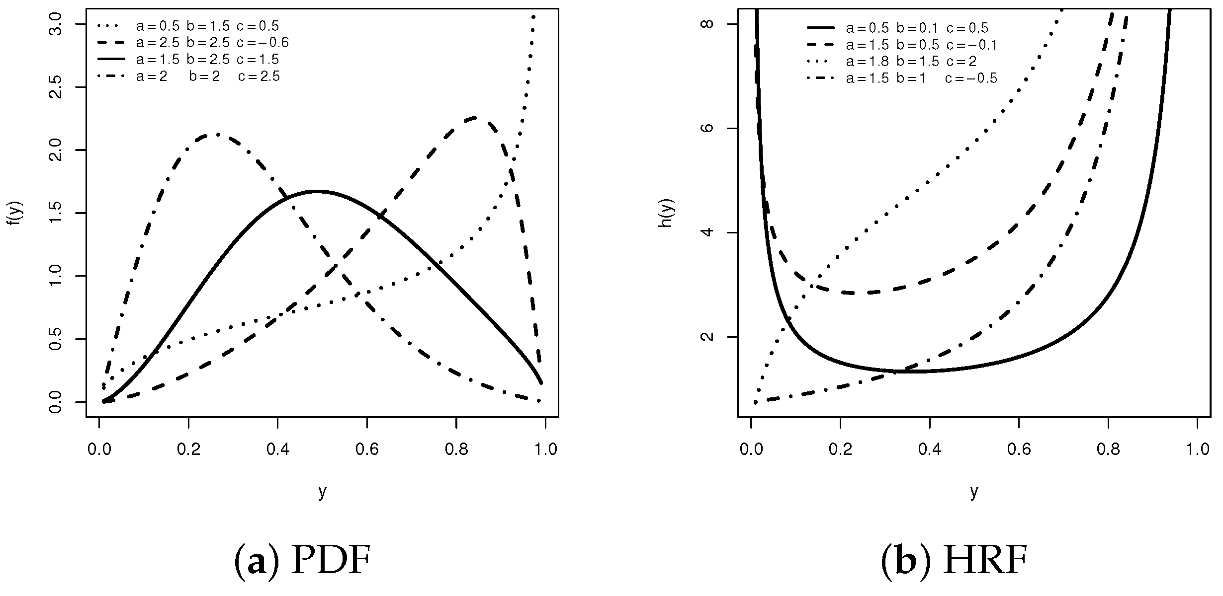
where a , b > 0 and 1 < c < . Taking various settings for the PNP ( α ) model, several shapes of its PDF and HRF are depicted in Figure 1. It exhibits that the PNP model features a flexible three-transaction structure, allowing it to capture a wide variety of distributional shapes, including increasing, decreasing, and bathtub hazard rates, as well as left/right-skewed, J-shaped, unimodal, and symmetric density patterns. These properties make the PNP lifetime distribution a robust and flexible tool for modeling bounded lifetime data, offering broad applicability across various practical and engineering domains. Karakaya et al. [1] also provided comprehensive analytical properties and finally concluded that the PNP lifespan represents a strong and practical statistical tool that improves model fit, estimation accuracy, and interpretability in real applications, outperforming several existing competitors such as Kumaraswamy, unit-Weibull, unit-Burr XII, and new power distributions. It also enables detailed statistical analysis, reliable parameter estimation using maximum likelihood and alternative methods, and accurate modeling of lifetime and proportional data. Overall, its flexibility and strong theoretical foundation make it a valuable tool for modern modeling and applied research.
Progressive first-failure censoring strategy (PFF-CS), originally proposed by Wu and Kuş [2], has emerged as an effective framework for addressing practical constraints in life-testing and reliability experiments, where complete observation of all failure times is often costly, time-intensive, or operationally infeasible. This mechanism combines two classical censoring mechanisms, namely, the first-failure censoring strategy (FF-CS) introduced by Balasooriya [3] and the Type-II progressive censoring strategy (PT2-CS) developed by Balakrishnan and Cramer [4]. In contrast to traditional approaches that require monitoring every failure, PFF-CS records only the earliest failure within each group, thereby substantially reducing experimental burden while preserving adequate statistical information for inference.
Specifically, n independent groups are formed, each consisting of s identical units, resulting in a total of n = n × s experimental units. At each stage, only the first failure time (symbolized by Y i : m : n for i = 1 , 2 , , m ) from the currently active group is recorded. Following this observation, a predetermined number of groups, denoted by R = ( R 1 , R 2 , , R m ) , are randomly withdrawn from the experiment in addition to the group in which the failure occurred. This sequential procedure continues until m ( n ) failure times are observed. For instance, upon observing the first failure Y 1 : m : n , the corresponding group together with R 1 additional groups is removed, leaving n R 1 1 groups under test. Likewise, after the second failure Y 2 : m : n , its associated group and R 2 further groups are eliminated, yielding n i = 1 2 R i 2 remaining groups. The process proceeds in this manner until the mth failure Y m : m : n is observed, after which all remaining groups, including the final failed group and R m additional groups, are removed. Despite its efficiency advantages in providing substantial experimental efficiency while preserving essential failure information, it assumes that the number of removed groups (denoted by R i for i = 1 , 2 , , m ) at each stage is fixed and known in advance. However, this assumption may be unrealistic in many practical situations.
However, most existing progressive censoring models assume that the number of units or groups removed at each stage is fixed in advance. Although mathematically convenient, this deterministic assumption may be overly restrictive in practical applications where unpredictable experimental constraints, environmental variability, or random operational factors often influence removals. In many engineering reliability studies, such as tensile strength analysis of advanced materials, the withdrawal of surviving groups may occur stochastically rather than according to a predetermined plan. Ignoring this randomness can reduce model realism and potentially affect inferential accuracy.
In reliability examinations on advanced materials such as carbon and polyester fibers, progressive withdrawals often occur naturally during testing. Grouped units typically undergo tensile strength tests, where they experience increasing stress until the first failure occurs in each group. After each failure, a random number of groups may be withdrawn due to practical constraints like equipment limits or specimen damage. This process is influenced by material-specific factors, such as brittle fracture and micro-cracking in carbon fibers, or environmental variability in polyester fibers, including humidity levels of 50–70% and temperatures of 20–30 °C, making the removal mechanism inherently stochastic.
In this context, several studies have extended PFF-CS by incorporating stochastic removal mechanisms instead of assuming fixed removals at each stage. Huang and Wu [5] considered a discrete-uniform removal mechanism. Although this approach introduces randomness into the withdrawal process, it implicitly assumes that all possible removal counts occur with equal probability, which may not adequately reflect practical experimental conditions. To provide additional flexibility, Ashour et al. [6] later proposed a binomial-based random removal design. However, the binomial formulation still relies on the assumption that the removal probability remains constant throughout the experiment. In many reliability and life-testing applications, such an assumption may be restrictive because withdrawal behavior is often influenced by changing operational conditions, experimental constraints, or environmental variability. To address this issue, Singh et al. [7] suggested modeling the removal probability itself as a random quantity following a beta distribution, leading naturally to the beta-binomial (BB) removal mechanism. This formulation allows the removal probabilities to vary across stages and therefore provides a more realistic representation of uncertainty in practical censoring experiments.
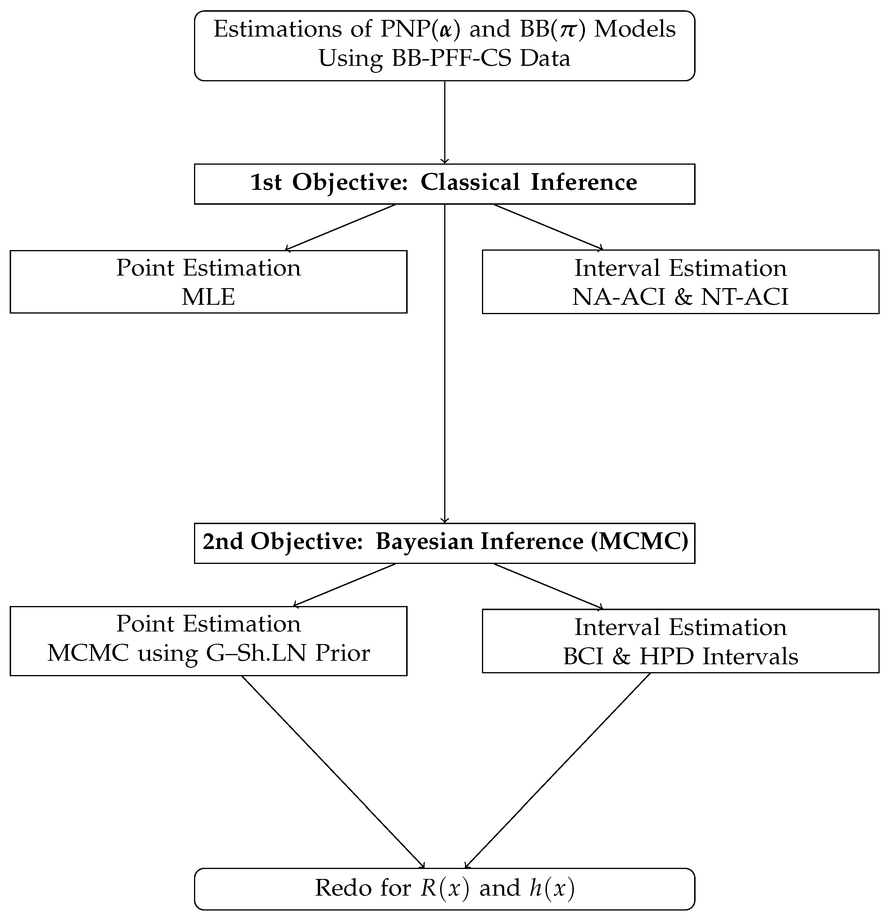
Motivated by these considerations, the present work develops a new reliability framework by integrating the BB framework through PFF-CS-based (BB-PFF-CS) with the flexible PNP lifetime distribution. To provide a clear high-level overview linking the estimation procedures and interval estimation methods, a simple flowchart is depicted in Figure 2.
Compared with existing deterministic and partially randomized censoring approaches, the proposed BB-PFF-CS framework offers greater adaptability in modeling bounded lifetime data under uncertain experimental conditions. From an inferential perspective, we develop comprehensive maximum likelihood and Bayesian estimation procedures for model parameters, reliability measures, and hazard characteristics. To bridge this gap, we contribute to this work with the following objectives:
  • A new framework is developed by combining the flexible PNP model via the BB-PFF-CS-based approach, allowing for a more realistic representation of experimental uncertainty.
  • Comprehensive classical inference procedures are developed, including maximum likelihood and asymptotic confidence interval methods.
  • A Bayesian setup is proposed using a joint gamma and shifted log-normal prior structure, which respects parameter constraints while maintaining flexibility and interpretability in prior specification. A sensitivity analysis of prior choices is performed, confirming the robustness and stability of the proposed Bayesian framework under different prior specifications.
  • Stochastic MCMC strategy based on the Metropolis–Hastings algorithm is designed to obtain Bayesian estimates and credible intervals for all model parameters and reliability measures.
  • Extensive Monte Carlo simulations are conducted to enhance computational efficiency and to evaluate estimator performance under various parameter settings and removal parameters.
  • Two reliability case studies, representing the tensile strength data of carbon and polyester fibers, are conducted to illustrate the practical applicability and improved modeling capability of the proposed method in engineering reliability contexts.
The rest of the paper is structured as follows. The proposed BB-PFF-CS is detailed in Section 2. Section 3 and Section 4 describe the likelihood and Bayesian frameworks, respectively. The outcomes of the simulation experiments are presented in Section 5. In Section 6, two tensile strength datasets are analyzed. Concluding remarks and final comments are provided in Section 7.

2. Description of the BB-PFF-CS Plan

Let y = { ( y 1 : m : n , r 1 ) , ( y 2 : m : n , r 2 ) , , ( y m : m : n , r m ) } represent the set of observed failure times gathered based on the BB-PFF-CS setup. It is assumed that the underlying lifetimes are independent and arise from a continuous distribution characterized by PDF f ( · ) and CDF F ( · ) . For notational convenience, we write y i y i : m : n . Subsequently, the likelihood function (LF) corresponding to the observed sample can be formulated as
L 1 α | r , y = Q 1 s m i = 1 m f y i ; α 1 F y i ; α r i 1 ,
where Q 1 = n n 1 r 1 n 2 i = 1 2 r i n m i = 1 m 1 r i and r i = s r i + 1 .
Assume that the number of removed groups r i at the ith observed failure, for i = 1 , 2 , , m 1 , follows a BB ( · ) law with parameters a and π , where a denotes the total number of trials and π = ( π 1 , π 2 ) is the vector of beta parameters. Consequently, the joint probability mass function of the BB removal vector r i for i = 1 , 2 , , m can be expressed as
L 2 R = r π = Q 2 B π 1 , π 2 m 1 i = 1 m 1 B π 1 + r i , π 2 + n r i ,
where Q 2 = n m ! n m i = 1 m 1 r i ! i = 1 m 1 r i ! and B π 1 , π 2 = Γ π 1 Γ π 2 Γ π 1 + π 2 .
Given that the random removals r i , for i = 1 , 2 , , m 1 , are assumed to be independent of the associated observed failure times y i , for i = 1 , 2 , , m 1 , the full-LF (say, L ( · ) ) can be constructed by combining the contributions from the lifetime component in (5) and the removal mechanism in (6) as follows:
L α , π y , r L 1 α y , r · L 2 r π .
It is important to note that the LF in (7) admits a decomposition into two terms, L i , i = 1 , 2 , each depending on distinct parameter sets, namely α and π . This separability implies that the corresponding parameters α and π can be estimated independently without loss of efficiency. Recently, several extensions of the PFF-CS have been proposed by incorporating random removal mechanisms called the discrete uniform (Huang and Wu [5]), binomial (Ashour et al. [6]), and BB (Elshahhat et al. [8]). These stochastic removal models provide a more realistic representation of uncertainty in unit withdrawals or eliminations, thereby enhancing the practical applicability of PT2-CS in reliability analysis. The relatively limited exploration of such models in the literature can be attributed to several challenges, including the complex structure of the resulting common probability function, the presence of a large number of tested parameters, and the computational complexity associated with the estimation procedures.

3. Classical Inference

This section is devoted to the classical point estimation and asymptotic interval inferences for the parameters of the PNP ( α ) and BB ( π ) models, based on data generated by the BB-PFF-CS. The same frequentist framework is further employed to estimate the RF R ( x ) and the HRF h ( x ) .

3.1. Point Estimation

Let y denote a BB-PFF-CS sample of size m, drawn from the PNP ( α ) distribution, whose PDF and CDF are given in (2) and (1), respectively. By substituting (2) and (1) into the LF (5), we get L 1 ( · ) as follows:
L 1 α | r , y a b m c + 1 m i = 1 m y i b 1 y i b a r i * 1 c y i b + 1 a r i * + 1 ,
where its natural logarithm expression becomes
log L 1 α | r , y m log a b + m log c + 1 + b i = 1 m log y i + i = 1 m a r i * 1 log 1 y i b i = 1 m a r i * + 1 log c y i b + 1 .
The MLEs of α , denoted by α ^ = ( a ^ , b ^ , c ^ ) , are acquired by simultaneous solving the system of three nonlinear equations formed from the first-order partial derivatives of the log-LF (8) with respect to each parameter, as expressed below:
m a + i = 1 m r i * log 1 y i b i = 1 m r i * log c y i b + 1 α = α ^ = 0 ,
m b + i = 1 m log y i i = 1 m i y i b log y i c i = 1 m ϑ i y i b log y i α = α ^ = 0 ,
and
m c + 1 i = 1 m ϑ i y i b α = α ^ = 0 ,
where i = a r i * 1 1 y i b 1 and ϑ i = a r i * + 1 c y i b + 1 1 .
It follows from Equations (10)–(12) that explicit closed-form expressions for α ^ cannot be derived. Therefore, numerical optimization procedures, such as the Newton–Raphson (NR) algorithm, are typically employed to obtain the estimates through iterative computation. Once the MLEs α ^ are determined, the invariance property of MLEs can be utilized to derive the corresponding estimates of the RF R ( x ) and the HRF h ( x ) by direct substitution. Accordingly, the MLEs of R ( x ) and h ( x ) , denoted by R ^ ( x ) and h ^ ( x ) , at x > 0 , are expressed as
R ^ ( x ; α ^ ) = 1 x b ^ c ^ x b ^ + 1 a ^ and h ^ ( x ; α ^ ) = a ^ b ^ ( c ^ + 1 ) x b ^ 1 ( 1 x b ^ ) ( a ^ c x b ^ + 1 ) ,
respectively.
Similarly, taking the natural logarithm of L 2 · in (6), we get:
log L 2 R = r π ( m 1 ) log Γ j = 1 2 π j ( m 1 ) log Γ ( π 1 ) + log Γ ( π 2 ) + i = 1 m 1 log Γ ( π 1 + r i ) + i = 1 m 1 log Γ ( π 2 + n * ) i = 1 m 1 log Γ r i + n * + j = 1 2 π j ,
where n * = n m j = 1 i r j . Accordingly, based on (13), the MLEs π ^ i , i = 1 , 2 , can be obtained by jointly solving the following system of nonlinear normal equations:
( m 1 ) ϕ j = 1 2 π j ϕ ( π 1 ) + i = 1 m 1 ψ ( π 1 + r i ) i = 1 m 1 ψ r i + n * + j = 1 2 π j π = π ^ = 0
and
( m 1 ) ψ j = 1 2 π j ψ ( π 2 ) + i = 1 m 1 ψ ( π 2 + n i * ) i = 1 m 1 ψ r i + n * + j = 1 2 π j π = π ^ = 0 ,
where ψ ( θ ) = θ log Γ ( θ ) is the digamma function.

3.2. Asymptotic Estimation

To construct the ( 1 μ ) 100 % asymptotic confidence interval (ACI) estimators for the unknown PNP parameters α , R ( x ) , and h ( x ) , in addition to the BB parameters π i , i = 1 , 2 , we rely on the large-sample properties of their corresponding MLEs.
According to standard regularity conditions, the estimator α ^ is asymptotically distributed as a multivariate normal with mean vector α and covariance-variance- matrix (CVM) given by Φ 1 1 ( · ) , where Φ 1 ( · ) represents the Fisher information matrix (FIM); see Lawless [9] for additional details. However, obtaining an explicit analytical expression for Φ 1 ( · ) is generally difficult due to the complicated structure of the second-order derivatives of the log-LF log L 1 ( · ) . Consequently, in practical implementation, the observed FIM evaluated at α ^ is employed as an approximation to Φ 1 1 ( · ) , and can be expressed as follows:
Φ ^ 1 1 ( α ^ ) = χ 11 χ 12 χ 13 χ 22 χ 23 χ 33 1 = ξ 11 ξ 12 ξ 13 ξ 22 ξ 23 ξ 33 ( α ^ = α ) ,
with
χ 11 = m a 2 , χ 22 = m b 2 i = 1 m y i b log y i i log y i + i c i = 1 m y i b log y i ϑ i log y i + ϑ i ,
χ 33 = m c + 1 2 i = 1 m ϑ i y i b , χ 12 = i = 1 m r i * i i 1 + i = 1 m r i * ϑ i ϑ i 1 ,
and
χ 13 = i = 1 m r i * y i b c y i b + 1 1 , and χ 23 = i = 1 m y i b log y i ϑ i + c ϑ i * ,
where
i = i y i b log y i 1 y i b 1 , ϑ i = ϑ i c y i b log y i c y i b + 1 1 ,
ϑ i = ϑ i y i b c y i b + 1 1 , and ϑ i * = y i b a r i * + 1 c y i b + 1 2 .
For constructing the ( 1 μ ) 100 % ACIs of R ( x ) and h ( x ) , it is essential to approximate the variances of the estimators R ^ ( x ) and h ^ ( x ) , symbolized by ξ ^ 44 and ξ ^ 55 , respectively. One of the most effective and commonly utilized approaches for this purpose is the delta method, which facilitates variance approximation for functions of estimated parameters. Interested readers may consult Greene [10] for a comprehensive treatment of this method. Applying the delta method yields the approximate variance expressions ξ ^ 44 and ξ ^ 55 for R ^ ( x ) and h ^ ( x ) , respectively, as given below:
ξ ^ 44 [ Σ R Φ ^ 1 1 ( α ) Σ R ] ( α ^ = α ) and ξ ^ 55 [ Σ h Φ ^ 1 1 ( α ) Σ h ] ( α ^ = α ) ,
where Σ R and Σ h are obtained and reported in Appendix A.
By setting π in the place of π ^ , the approximated CVM of the BB parameters π (say, Φ ^ 2 1 ( · ) ) becomes
Φ ^ 2 1 ( π ^ ) = χ 66 χ 67 χ 77 1 = ξ 66 ξ 67 ξ 77 ( π ^ = π ) ,
with items, χ i j , i , j = 6 , 7 , are:
χ 66 = ( m 1 ) ϕ π 1 Γ π 1 ϕ π 1 + π 2 Γ π 1 + π 2 + i = 1 m 1 ϕ π 1 + r i Γ π 1 + r i i = 1 k 1 ϕ ϱ i Γ ϱ i ,
χ 77 = ( m 1 ) ϕ π 2 Γ π 2 ϕ π 1 + π 2 Γ π 1 + π 2 + i = 1 m 1 ϕ π 2 + n * Γ π 2 + n * i = 1 m 1 ϕ ϱ i Γ ϱ i ,
and
χ 67 = ( m 1 ) ϕ π 1 + π 2 Γ π 1 + π 2 i = 1 m 1 ϕ ϱ i Γ ϱ i ,
where ϱ i = π 1 + π 2 + n * + r i and ϕ ρ θ = t ϕ ρ θ is the trigamma function.
Due to the likelihood equations corresponding to the PNP ( α ) and BB ( π ) models not admitting explicit closed-form solutions, numerical procedures such as the NR method are recommended for evaluating the elements χ i j , i , j = 1 , , 7 , appearing in the CVMs in (16) and (18). Relying on the normal approximation (NA) of the MLEs for a, b, c, R ( x ) , and h ( x ) , the corresponding two-sided ( 1 μ ) 100 % ACI bounds at significance level μ can be constructed. Accordingly, for any parameter or function of interest (a, b, c, R ( x ) , h ( x ) , or π i , i = 1 , 2 denoted generically by ξ ), the NA-based ACI (NA-ACI) is given by
ξ ^ i ± z 0.5 μ ξ ^ i i , i = 1 , 2 , , 7 ,
where ξ 1 , ξ 2 , ξ 3 , ξ 4 , ξ 5 , ξ 6 , ξ 7 = a , b , c , R ( x ) , h ( x ) , π 1 , π 2 and z 0.5 μ is the upper 0.5 μ th percentile point of the standard Gaussian distribution.
One key limitation of the conventional NA-ACI method is that it can produce lower bounds that fall outside the feasible parameter space, particularly for parameters restricted to positive values. While a common remedy is to truncate the interval at zero, this adjustment is empirical and lacks formal inferential justification. To address this issue and guarantee that the confidence intervals respect the parameter domain, Meeker and Escobar [11] introduced the normal log-transformed ACI (NT-ACI). Accordingly, the ( 1 μ ) 100 % NT-ACI for a given parameter or function ξ is expressed as
ξ ^ i exp z 0.5 μ ξ ^ i 1 ξ ^ i i , i = 1 , 2 , , 7 .

4. Bayesian Inference

In this section, we outline the Bayesian estimation framework for the PNP and BB model parameters under BB-PFF-CS data, encompassing α , R ( x ) , h ( x ) , and π .

4.1. Prior Specification

We begin by assigning prior distributions to the PNP shape parameters a and b, as well as to the BB parameters π 1 and π 2 , all of which are assumed to be mutually independent a priori and are modeled using gamma prior distributions. In contrast, for the parameter c, whose support extends over ( 1 , ) , a shifted log-normal (Sh.LN) prior is adopted to properly accommodate its domain while preserving flexibility in prior modeling.

4.1.1. Gamma Prior

The use of gamma priors is motivated by several desirable statistical and computational properties. In particular, for the strictly positive parameters a, b, π 1 , and π 2 , gamma priors are appropriate because
(i)
They naturally satisfy positivity constraints;
(ii)
They are highly flexible and can represent a wide range of prior beliefs, from weakly informative to moderately informative structures, through suitable hyperparameter choices;
(iii)
They are widely used in reliability and survival analysis and often provide numerically stable posterior computations.
Accordingly, for the PNP ( α ) model, the joint prior PDF of a and b, denoted by Υ 1 ( · ) , is defined as the product of two independent gamma distributions, specifically G a ( ϵ 1 , ε 1 ) and G b ( ϵ 2 , ε 2 ) . Thus, the joint prior density of a and b is given by
Υ 1 ( a , b ) a ϵ 1 1 b ϵ 2 1 exp ( ε 1 a + ε 2 b ) , a , b > 0 ,
where ϵ i > 0 and ε i > 0 for i = 1 , 2 are known hyperparameters that may be selected based on prior knowledge or chosen to reflect weak prior knowledge. Similarly, for the BB ( π ) model parameters, independent gamma priors are assigned to π 1 and π 2 , denoted by G π 1 ( ϵ 3 , ε 3 ) and G π 2 ( ϵ 4 , ε 4 ) , respectively. Therefore, the joint gamma prior density of π becomes
Υ 2 ( π ) π 1 ϵ 3 1 π 2 ϵ 4 1 exp ( ε 3 π 1 + ε 4 π 2 ) , π i > 0 , i = 1 , 2 ,
where ϵ i > 0 and ε i > 0 for i = 3 , 4 also assumed to be known.

4.1.2. Shifted Log-Normal Prior

For the parameter c, whose support is restricted to ( 1 , ) , a shifted log-normal prior is employed through the transformation
c = 1 + exp ( η ) , η N ( μ , σ 2 ) .
This transformation in (23) guarantees that all posterior realizations satisfy the theoretical support condition c > 1 , while also enabling Bayesian computation on an unconstrained scale. Such transformation-based prior structures are commonly recommended for constrained parameters; see, for example, Bernardo et al. [12] and Gelman et al. [13]. Under this specification, the prior density of c is
Υ 3 ( c ) = 1 ( c + 1 ) σ 2 π exp log ( c + 1 ) μ 2 2 σ 2 , c > 1 .
The shifted log-normal prior offers several important advantages:
(i)
It strictly enforces the support restriction c > 1 , thereby preventing infeasible parameter values during posterior simulation;
(ii)
It provides substantial flexibility, including right-skewed behavior, which is often appropriate for reliability-related parameters;
(iii)
The hyperparameters μ and σ 2 have intuitive interpretations on the log scale, facilitating practical prior elicitation;
(iv)
It improves numerical stability and computational efficiency in MCMC implementation.
Overall, the joint Gamma and Sh.LN (G-Sh.LN) priors framework achieves a balanced integration of theoretical validity, modeling flexibility, and computational tractability. It also ensures that the prior assumptions align with the structural constraints of the proposed model.
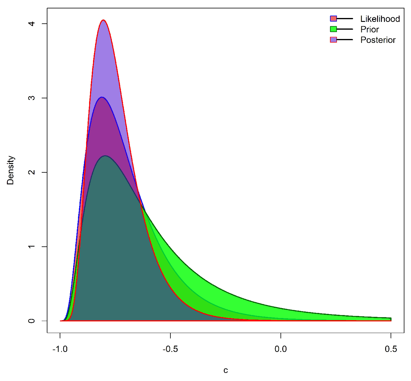
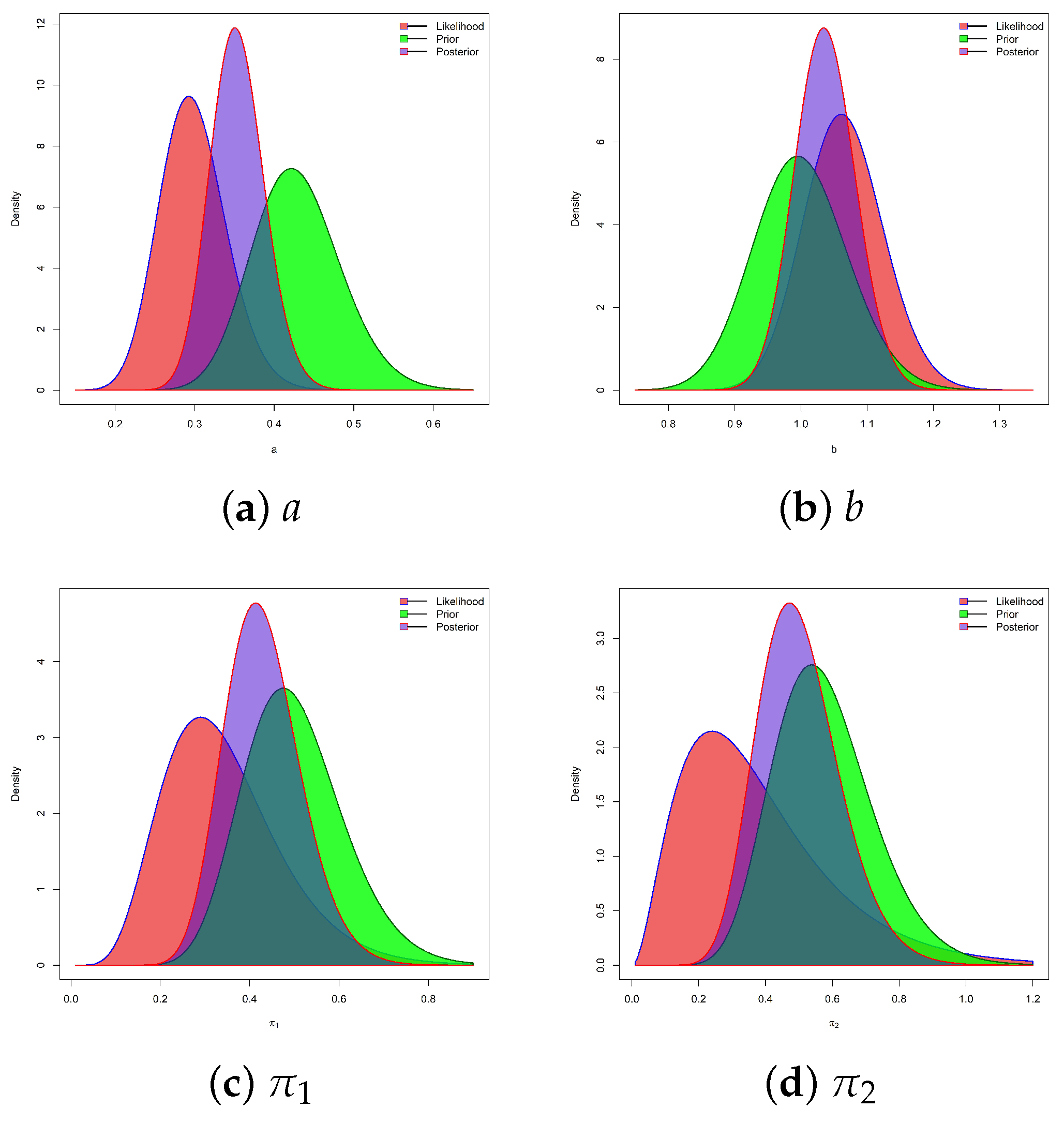
Additionally, the graphical comparison of the likelihood, prior, and posterior densities in Figure 3 and Figure 4, from PNP ( 0.5 , 1.0 , 0.5 ) (as an example), provides important insights into the adequacy and behavior of the selected prior distributions for both the PNP and BB model parameters. For the parameters a and b of the PNP model, as well as the BB parameters π 1 and π 2 , the gamma prior specification appears highly appropriate. To highlight it, the plotted densities in Figure 3 show that:
1.
The priors for a, b, π 1 , and π 2 are reasonably diffuse compared to the likelihoods, indicating that they do not dominate the data but instead provide mild regularization. These also provide substantial flexibility in capturing various shapes (e.g., skewed or near-symmetric forms), allowing both informative and weakly informative prior settings.
2.
The posterior outcomes concentrated and shifted toward the likelihood peaks, reflecting a coherent balance between prior beliefs and observed information. This behavior confirms that the gamma priors help stabilize estimation without introducing undue bias.
3.
Finally, from a Bayesian computational perspective, gamma priors led to analytically tractable or numerically stable posterior updates.
For the parameter c, Figure 4 reveals that the Sh.LN prior structure naturally accommodates skewness, as evident in the plotted densities, where both the likelihood and posterior exhibit asymmetric behavior. It is relatively spread out, indicating weak prior informativeness, while the posterior is appropriately concentrated, suggesting that the data play a dominant role in inference. It also lies in its reparameterization on the log scale, which improves numerical stability and efficiency in Bayesian computation, particularly in MCMC-based estimation.
Overall, the joint use of gamma priors for ( a , b , π 1 , π 2 ) and a Sh.LN prior for c provides a coherent and practically effective prior specification. The chosen priors respect the natural parameter constraints, offer sufficient flexibility to model uncertainty, and lead to well-behaved posterior distributions, as clearly supported by the graphical evidence. This combination, therefore, represents a sound and reliable Bayesian modeling strategy for the proposed BB-PFF-CS framework.

4.2. Posterior Density

This subsection introduces the MCMC estimators and associated BCI/HPD bounds of α , R ( x ) , and h ( x ) for the PNP model as well as of π for the BB model. From (8), (21), and (24), the joint posterior PDF (say, Π 1 ( · ) ) of a, b, and c is
Π 1 ( α | r , y ) a m + ϵ 1 1 b m + ϵ 2 1 c + 1 m 1 e ( ε 1 a + ε 2 b ) e ( log ( c + 1 ) μ ) 2 2 σ 2 i = 1 m y i b B i ( a , b , c ) ,
with
B i ( a , b , c ) = 1 y i b a r i * 1 c y i b + 1 a r i * + 1 ,
where its normalized term (say, A 1 ) is given by
A 1 = 0 0 0 L 1 α | r , y × Υ 1 ( a , b ) × Υ 3 ( c ) d a d b d c .
From (6) and (22), the joint posterior PDF of the BB ( π ) model, say Π 2 ( · ) , becomes
Π 2 R = r π = A 2 1 π 1 ϵ 3 1 π 2 ϵ 4 1 e ( ε 3 π 1 + ε 4 π 2 ) B π 1 , π 2 m 1 i = 1 m 1 B π 1 + r i , π 2 + n r i ,
where
A 1 = 0 0 L 2 R = r π × Υ 2 ( π ) d π 1 d π 2 .
Owing to the nonlinear structure of the posterior distribution Π 1 ( · ) given in (25), explicit analytical forms for the Bayes estimators of α , R ( x ) , and h ( x ) are not obtainable. Therefore, Markov Chain Monte Carlo (MCMC) methods are employed to approximate these estimators and to construct the corresponding Bayesian credible interval (BCI) and highest posterior density (HPD) interval estimators for each unknown quantity.
To implement this approach, it is necessary to first derive the full conditional posterior density functions of the PNP model parameters a, b, and c, which are given as follows:
Π 1 a ( a | b , c , r , y ) a m + ϵ 1 1 e ε 1 a i = 1 m B i ( a , b , c ) ,
and
Π 1 b ( b | a , c , r , y ) b m + ϵ 2 1 e ε 2 b i = 1 m y i b B i ( a , b , c ) ,
and
Π 1 c ( c | a , b , r , y ) c + 1 m 1 e ( log ( c + 1 ) μ ) 2 2 σ 2 i = 1 m B i ( a , b , c ) ,
respectively.
It follows from (27) and (28) that the full conditional posterior distributions of the parameters a, b, and c do not admit closed-form expressions corresponding to any standard distribution. Consequently, direct sampling from the conditional densities Π 1 a ( · ) , Π 1 b ( · ) , and Π 1 c ( · ) using conventional methods is not practical. To overcome this difficulty, the Metropolis–Hastings (MH) algorithm is implemented with Gaussian proposal distributions to simulate draws from the target posteriors. Remember that Figure 3 and Figure 4 show that the posterior outcomes of a, b, and c, obtained from (27), (28), and (29), respectively, exhibit behavior similar to the Gaussian model. This sampling strategy facilitates the computation of Bayes estimates as well as the construction of credible intervals for all PNP model parameters; see Algorithm 1.
Algorithm 1 The MCMC (MH-based) Generation Steps
1:
Input: Start with j = 1
2:
Input: Set α α ^
3:
Output: Get a from N ( a ^ , ξ ^ 11 )
4:
Output: Calculate a = min 1 , Π 1 a a | b j 1 , c j 1 , y Π 1 a a j 1 | b j 1 , c j 1 , y
5:
Output: Get a uniform variate (say, u) from U ( 0 , 1 )
6:
Output: Store a
7:
As a ( j )
8:
if   u a  then
9:
   Else set a ( j 1 )
10:
end if
11:
Input: Redo Steps 3–10 for b ( j ) from Π 1 b and c ( j ) from Π 1 c
12:
Output: Obtain R ( j ) ( x ) from (3) and h ( j ) ( x ) from (4)
13:
Input: Set j = j + 1
14:
Input: Redo Steps 1–13 δ times, and remove a burn-in size (say, δ )
15:
Output: Compute the Bayesian estimate of a (say, a ˜ ) via the squared error loss (SEL) as:
a ˜ = 1 δ j = δ + 1 δ a ( j ) ,
where δ = δ δ
16:
Input: Sort a ( j ) (for j = δ + 1 , δ + 2 , , δ )
17:
Output: Compute the 100 ( 1 μ ) % BCI bounds of a as:
a 0.5 μ δ , a ( 1 0.5 μ ) δ
18:
Output: Compute the ( 1 μ ) 100 % HPD interval of a as:
a ( j ) , a ( j + ( 1 μ ) δ )
where j is the index that minimizes:
a j + ( 1 μ ) δ a ( j ) for j = 1 , , j δ
19:
Output: Redo Steps 15–18 for b, c, R ( x ) , and h ( x )
In a similar fashion, from (26), the full-conditional posterior PDFs of the BB model parameters π i , i = 1 , 2 , can be formulated, respectively, as
Φ 2 π 1 π 1 π 2 , R = r π 1 ϵ 3 1 e ε 3 π 1 B π 1 , π 2 k 1 i = 1 k 1 B π 1 + r i , π 2 + n * ,
and
Φ 2 π 2 π 2 π 1 , R = r π 2 ϵ 4 1 e ε 4 π 2 B π 1 , π 2 k 1 i = 1 k 1 B π 1 + r i , π 2 + n * .
As anticipated from (30) and (31), the conditional posterior distributions of π i , i = 1 , 2 , cannot conform to any known statistical standard form. Accordingly, it is not feasible to draw samples directly from these distributions using standard sampling techniques. Again, Figure 3 states that the posterior outcomes of both BB coefficients π i , i = 1 , 2 obtained from (30) and (31), respectively, exhibit behavior similar to the Gaussian model. Subsequently, we re-recommend applying the MH algorithm once more, following the procedure outlined in Algorithm 1, to generate MCMC samples for π i , i = 1 , 2 .

5. Monte Carlo Comparisons

This section presents a detailed numerical evaluation of the proposed inferential framework, focusing on both point and interval estimation of the PNP ( a , b , c ) model parameters, as well as the associated reliability characteristics, namely the RF R ( x ) and HRF h ( x ) .

5.1. Simulation Frameworks

The study is conducted using two independent lifetime populations generated from the PNP ( α ) model, specifically Pop-1:PNP ( 0.5 , 1.0 , 0.5 ) and Pop-2:PNP ( 1.5 , 2.0 , 1.5 ) . A Monte Carlo simulation scheme is implemented by replicating the BB-PFF-CS mechanism 2000 times. Objective samples of the PNP model are created within the proposed control framework according to the procedure outlined in Algorithm 2. The inferential analysis of the reliability measures is carried out at the fixed point x = 0.1 . For the two parameter settings considered (Pop-i for i = 1 , 2 ), the true values of R ( x ) are 0.9733 and 0.9633, while the corresponding values of h ( x ) are 0.2923 and 0.7464, respectively. The performance of the resulting estimators for a, b, c, R ( x ) , and h ( x ) is examined under a variety of experimental configurations defined by the group size s, total number of test units n, number of observed failures m, and the BB parameters ( π 1 , π 2 ) . In particular, the group size is fixed at s = 2 and 5, while the number of groups is taken as n = 20 , 50 , and 80. To further investigate the impact of the removal scheme, two different BB settings are considered, namely BB-1: ( 0.5 , 0.5 ) and BB-2: ( 1.5 , 1.5 ) .
Algorithm 2 Generate Steps of BB-PFF-CS Data
1:
Input: Specify the PNP ( a , b , c ) model parameters
2:
Input: Specify the BB ( π 1 , π 2 )
3:
Input: Fix the censoring controls s, n, and m
4:
Step 1: Generate the first removal count r 1 from B B n m , π 1 , π 2
5:
Step 2: For i = 2 , 3 , , m 1 , generate
r i B B n m j = 1 i 1 r j , π 1 , π 2
6:
Step 3: Compute r m as
r m = n m i = 1 m 1 r i , if n m i = 1 m 1 r i > 0 , 0 , otherwise
7:
Step 4: Generate independent random variables B i U ( 0 , 1 ) for i = 1 , 2 , , m
8:
Step 5: Construct
A i = B i i + j = m i + 1 m r j 1 , i = 1 , 2 , , m
9:
Step 6: Set
U i = k = 0 i 1 A m k , i = 1 , 2 , , m
10:
Step 7: Set
U i = 1 U i , i = 1 , 2 , , m
11:
Step 8: Find
y i = F 1 U i ; α , i = 1 , 2 , , m
12:
Output: Get BB-PFF-CS sample { y 1 , , y m }
Following the MCMC strategy described in Section 4, a total of = 12,000 iterations is generated, with the first = 2000 samples discarded as burn-in. The remaining draws are then used to compute posterior summaries along with the corresponding 95% BCI and HPD interval estimates for all model parameters and reliability measures. For the numerical implementation, 2000 BB-PFF-CS datasets are generated, and the analysis is carried out using the R programming environment. In particular, the maxLik package (by Henningsen and Toomet [14]) is employed for ML estimation and its associated 95% NA-ACI and NT-ACI methods, while posterior simulation and its associated 95% BCI and HPD methods are performed using the coda package (by Plummer et al. [15]). A critical aspect of Bayesian analysis lies in the appropriate specification of prior hyperparameters. In this work, we adopt the prior-elicitation strategy for the joint G-Sh.LN prior distribution proposed; following Kundu [16], we determine the hyperparameters ϵ i and ε i for ( i = 1 , 2 ) associated with ( a , b ) as well as ( μ , σ ) associated with c as follows:
  • For Pop-1: Taking ( μ , σ 2 ) = ( 1.193 , 1 ) of c, we set:
    -
    Prior–1[P1]: ( ϵ 1 , ϵ 2 ) = ( 2.5 , 5 ) and ε i = 5 , i = 1 , 2 ;
    -
    Prior–2[P2]: ( ϵ 1 , ϵ 2 ) = ( 5.0 , 10 ) and ε i = 10 , i = 1 , 2 ,
  • For Pop-2: Taking ( μ , σ 2 ) = ( 0.416 , 1 ) of c, we set:
    -
    Prior–1[P1]: ( ϵ 1 , ϵ 2 ) = ( 7.5 , 10 ) and ε i = 5 , i = 1 , 2 ;
    -
    Prior–2[P2]: ( ϵ 1 , ϵ 2 ) = ( 15 , 20 ) and ε i = 10 , i = 1 , 2 .
For more specifications on the specified values provided in Pi (for i = 1 , 2 ), the mean expressions of ( a , b ) and c are given, respectively, by
E ( a ) = ϵ 1 ε 1 , E ( b ) = ϵ 2 ε 2 , and E ( c ) = 1 + exp μ + σ 2 2 .

5.2. Sensitivity Analysis

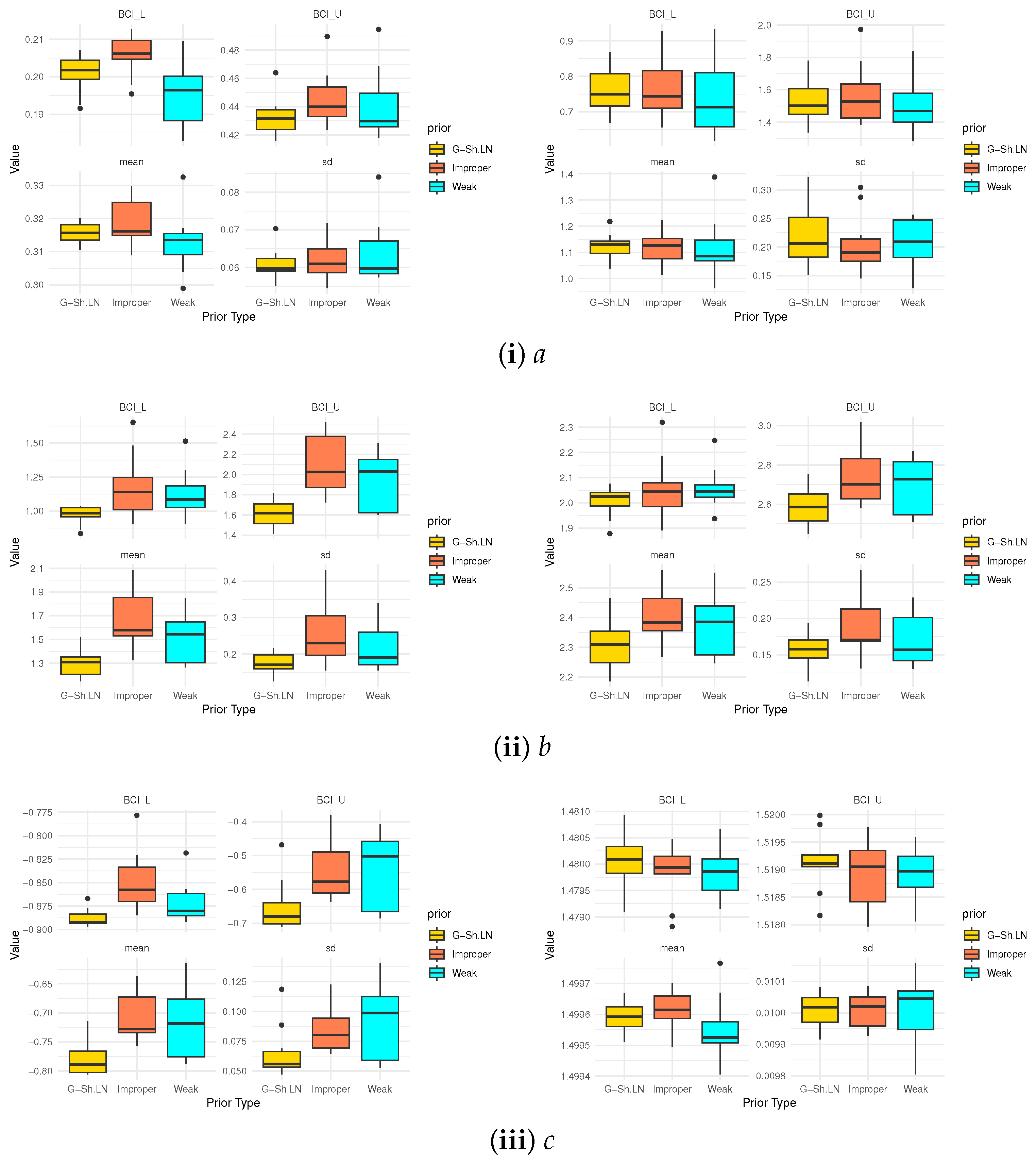
Sensitivity maps serve primarily as a visual and quantitative tool to illustrate how posterior summaries, including means, standard deviations, and credible interval limits, respond to alternative prior specifications. In applied contexts, such as medicine or engineering, knowing that posterior inferences are stable under plausible variations in the prior increases the reliability of subsequent decisions or predictions based on the model. Figure 5 provides a comprehensive assessment of the robustness of the Bayesian estimators of the parameters a, b, and c under different prior specifications, namely the proposed joint G-Sh.LN prior, weakly informative priors, and improper priors.
Overall, the results indicate that the proposed G-Sh.LN prior yields more stable and concentrated posterior summaries across both populations. In particular, the posterior means of a, b, or c, under the G-Sh.LN prior, remain consistently close to each other with relatively smaller variability, while the associated BCI limits tend to be shorter compared to those obtained under weak and improper priors. This behavior suggests improved estimation efficiency and reduced posterior uncertainty. In contrast, the improper prior often leads to increased dispersion and, in some cases, noticeable shifts in posterior location, reflecting its sensitivity to the likelihood structure. The weak prior exhibits intermediate performance but still shows wider interval estimates relative to the proposed prior. Notably, the robustness pattern is consistent across both Pop-i for i = 1 , 2 with the gamma prior parameters ϵ i and ε i for ( i = 1 , 2 ) of ( a , b ) as well as with the Sh.LN prior parameters ( μ , σ ) of c, although the effect is more pronounced for parameter c, where the Sh.LN prior plays a crucial role in stabilizing inference. By confirming the stability of parameter estimates across a range of prior assumptions, this analysis reinforces confidence in the applicability of the joint G–Sh.LN prior for diverse populations and supports its use for decision-making in practice.
We next assess the accuracy of the point and interval estimators corresponding to the model parameters a, b, and c, as well as the reliability measures R ( x ) and h ( x ) . For notational convenience, let ð denote any of these quantities. The evaluation is carried out using the following metrics:
  • Root mean squared-error (RMSE):
    RMSE ( ð ˇ ) = 1 2000 ı = 1 2000 ð ˇ [ ı ] ð 2 ,
  • Average absolute bias (AAB):
    AAB ( ð ˇ ) = 1 2000 ı = 1 2000 ð ˇ [ ı ] ð ,
  • Average interval length (AIL):
    AIL 95 % ( ð ) = 1 2000 ı = 1 2000 U ð ˇ [ ı ] L ð ˇ [ ı ] ,
  • Coverage percentage (CP):
    CP 95 % ( ð ) = 1 2000 ı = 1 2000 D L ð ˇ [ ı ] ; U ð ˇ [ ı ] ð ,
    where ð ˇ [ ı ] is the fitted estimate of ð at the ıth sample.

5.3. Convergence Diagnostics

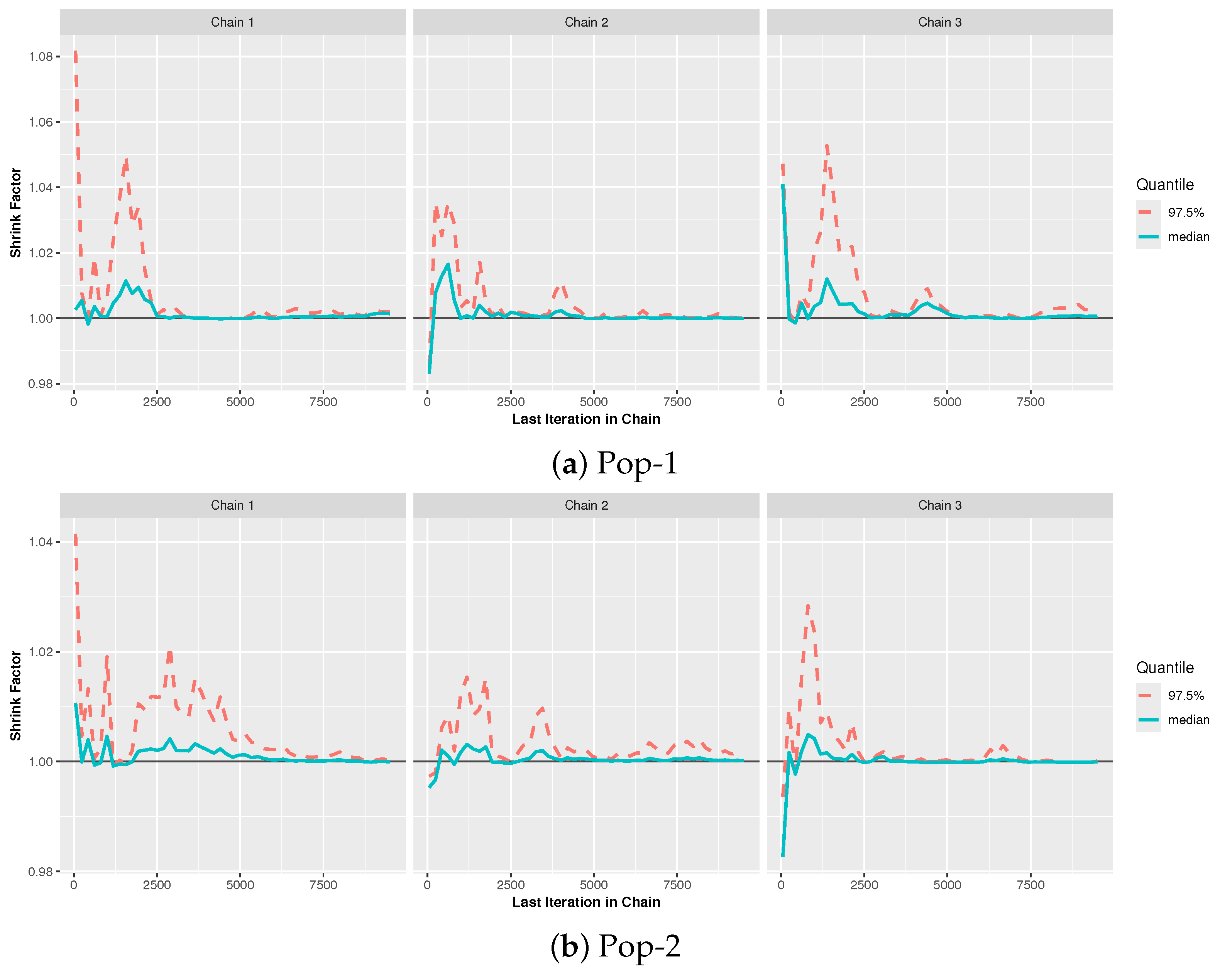
Figure 6 presents the Brooks–Gelman–Rubin (BGR) convergence diagnostics for multiple MCMC chains from Pop-i, i = 1 , 2 , providing a visual assessment of chain mixing and convergence stability. Across all chains, the potential scale reduction factors rapidly approach unity, indicating strong agreement between within-chain and between-chain variances. The median trajectories stabilize quickly, while the upper quantile (97.5%) exhibits only minor initial fluctuations before converging, reflecting limited early-stage variability during the burn-in period. This behavior confirms that the selected burn-in length is adequate and that the chains show no evidence of persistent non-convergence. Consequently, these diagnostics support the reliability of posterior inference under the proposed Bayesian framework.
To ensure efficient posterior sampling, Gaussian random-walk proposal distributions were constructed for parameters a, b, and c, centered at their current states, with initial proposal variances derived from the inverse observed FIM. Because the posterior geometry of the PNP-BB-PFF-CS model may exhibit skewness, parameter dependence, or local irregularities, acceptance rates were carefully monitored during pilot runs and adaptively tuned to achieve desirable sampling efficiency. Specifically, the observed average acceptance rates ranged approximately from 72–85% for a, 80–89% for b, and 75–87% for c. These acceptance rates indicate stable chain movement, satisfactory posterior exploration, and efficient sampling performance under the chosen proposal structure.
During the pilot tuning stage, proposal variances were iteratively adjusted to improve mixing behavior and maintain computational stability. In particular, proposal scales were reduced when acceptance rates fell below 40% and increased when acceptance rates exceeded 70%, with tuning continuing until stable acceptance behavior within the target range of approximately 60–80% was achieved. Once satisfactory tuning was established, the optimized proposal variances were fixed for the main MCMC runs to preserve the theoretical validity and stationary properties of the Markov chains while ensuring efficient posterior sampling.
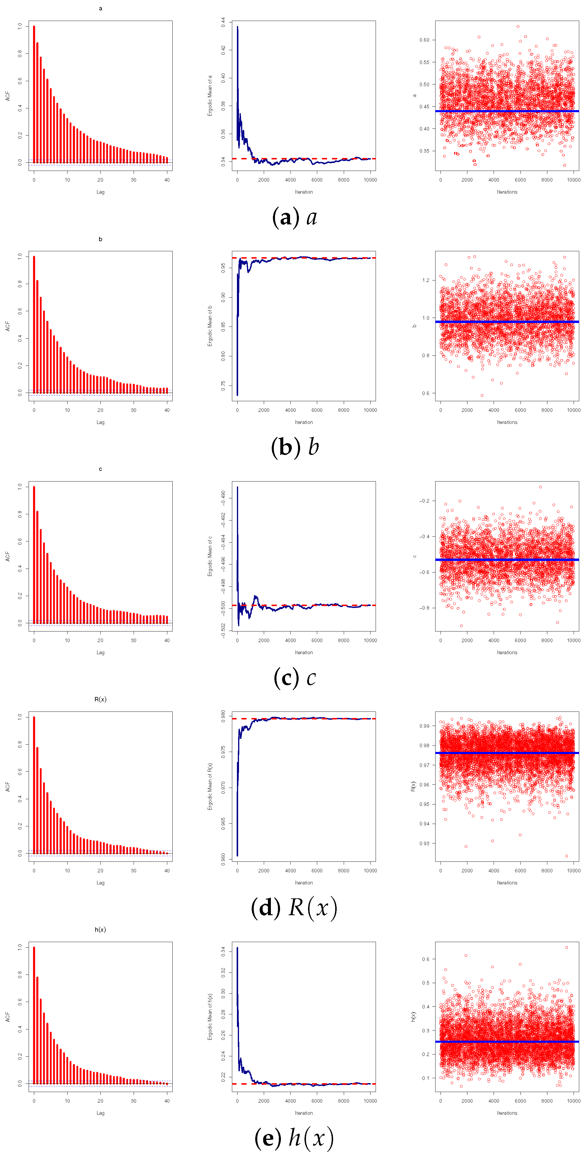
For Pop-1 as a representative example, Figure 7 displays key diagnostic plots, including trace plots, autocorrelation functions (ACF), and ergodic mean plots. These diagnostics collectively demonstrate satisfactory convergence, low serial dependence, and stable posterior estimation across iterations. For clarity, the horizontal reference lines in Figure 7b,c represent the corresponding posterior mean estimates.

5.4. Prior Robustness Analysis

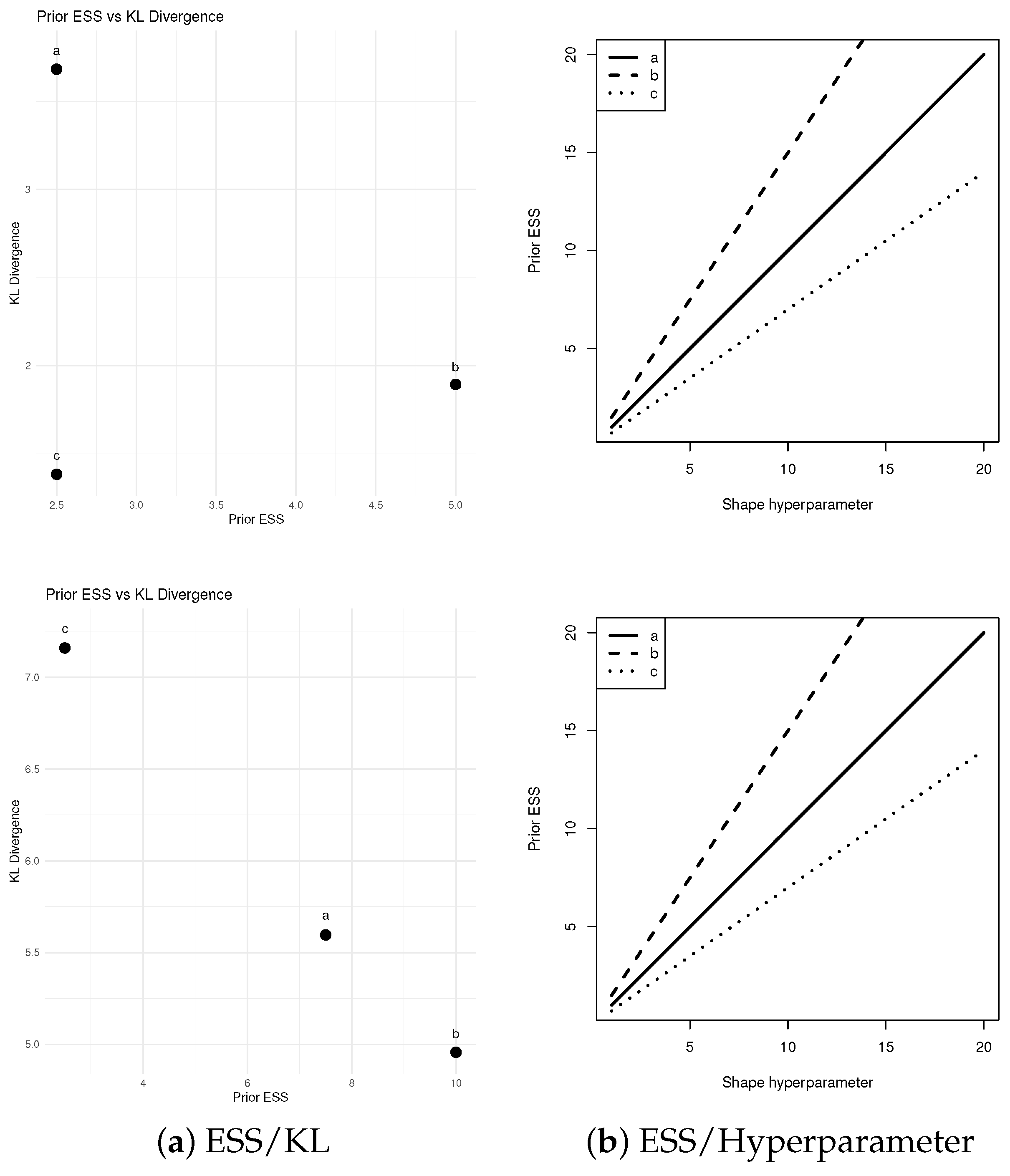
To further safeguard against prior misspecification and excessive posterior confidence, we complement sensitivity analysis with quantitative diagnostics based on prior effective sample size (Prior-ESS) and Kullback-Leibler (KL) divergence between prior and posterior distributions; see Figure 8. For clarification, Prior-ESS provides an interpretable measure of the relative informativeness contributed by each prior, while KL divergence quantifies the degree to which observed data update prior beliefs.
Figure 8a assesses the relationship between prior informativeness and posterior learning by jointly evaluating Prior-ESS and KL divergence. For Pop-1, parameters a and c exhibit relatively modest Prior-ESS values (2.5), accompanied by substantial KL divergences of 3.6839 and 1.3832, respectively, indicating that posterior inference remains primarily data-driven despite prior regularization. Parameter b, with a slightly larger ESS value (5.0), shows moderate KL divergence (1.89), suggesting balanced prior influence without excessive dominance. Similarly, for Pop-2, although Prior-ESS values for a and b increase to 7.5 and 10, the corresponding KL divergences (5.59 and 4.95) remain substantial, confirming strong posterior learning and limited prior overreach. The parameter c, despite a lower ESS value (2.5), exhibits the highest KL divergence (7.15), further emphasizing substantial data contribution. As a result, across both Pop-1 and Pop-2, these diagnostics confirm that the proposed priors do not excessively dominate the likelihood.
Figure 8b provides an additional practical guideline by illustrating how Prior-ESS evolves as prior shape hyperparameters increase. The approximately linear growth patterns demonstrate that prior informativeness strengthens systematically with hyperparameter concentration, although at different rates across parameters. In particular, b exhibits the fastest ESS growth, followed by a, while c remains comparatively less sensitive.
Finally, we recommend selecting hyperparameter values that maintain Prior-ESS within moderate ranges relative to sample size, particularly when prior knowledge is uncertain. Hyperparameter concentration should be increased gradually, while jointly monitoring KL divergence and posterior interval behavior to ensure continued robustness. This combined diagnostic framework provides both pre-estimation and post-estimation safeguards, enabling practitioners to balance efficiency and robustness while minimizing the risk of prior-induced overconfidence.

5.5. Simulation Results and Interpretation

The numerical results for point estimation of the parameters a, b, c, R ( x ) , and h ( x ) are summarized in Table 1, Table 2, Table 3, Table 4 and Table 5. In contrast, for the same unknown subjects, Table 6, Table 7, Table 8, Table 9 and Table 10 present the interval estimation results. Upon these results, the competing estimation methods are evaluated according to smaller values of RMSE, AAB, and AIL, together with larger values of CP. The principal findings can be summarized as follows:
  • The proposed estimation procedures, for both point and interval inference of a, b, c, R ( x ) , and h ( x ) , exhibit stable and reliable performance across all simulated configurations.
  • An increase in n leads to enhanced estimation accuracy for all considered methods, indicating improved statistical efficiency as more failure information becomes available.
  • When evaluating the joint G-Sh.LN prior, Bayesian results consistently demonstrate superior performance compared to frequentist results due to the incorporation of prior information.
  • Comparing the four interval estimation frameworks. In particular, both BCI and HPD estimations generally achieve shorter AILs and higher CPs compared to NA-ACI and NT-ACI estimations. Moreover, BCI/HPD methods constructed by P2 provide more accurate and stable interval estimates than those based on P1, which is consistent with the increased precision associated with more informative priors.
  • All Bayesian outcomes obtained under P2 consistently outperform those based on P1. This improvement can be attributed to the higher informativeness of P2, reflected in its relatively smaller variance.
  • Increasing the PNP parameters α yields:
    -
    The RMSE, AAB, and AIL results of all unknown quantities increased, except the AILs of b.
    -
    The CP results of a, c, R ( x ) , and h ( x ) narrowed down, whereas those corresponding to b increased.
  • Increasing the group size s yields:
    -
    The RMSE and AAB results of a, R ( x ) , and h ( x ) increased, while those of b and c narrowed down;
    -
    The AIL results of a, c, and R ( x ) increased, while those of b and h ( x ) decreased;
    -
    The CP results of b and h ( x ) tend to increase, whereas those corresponding to a, c, and R ( x ) decreased.
    -
    For ML-based estimation, the RMSE and AAB associated with a, R ( x ) , and h ( x ) tend to increase, whereas those corresponding to b show a decreasing trend;
    -
    For MCMC-based Bayesian estimation, both RMSE and AAB increase for all parameters;
    -
    The AILs of both asymptotic and credible intervals increase for a, while they decrease for b, R ( x ) , and h ( x ) ;
    -
    The CPs of all proposed intervals improve for b, R ( x ) , and h ( x ) , whereas a slight deterioration is observed for a.
  • As the BB parameters π i , i = 1 , 2 , increase, the following patterns are observed:
    -
    The RMSE and AAB results increase for a, b, c, and h ( x ) , while a decreasing trend is noted for R ( x ) ;
    -
    The AIL results of a, b, and h ( x ) increased, while those of c and R ( x ) decreased;
    -
    The CPs associated with c and R ( x ) grow, whereas those corresponding to a, b, and h ( x ) tend to decrease.
  • The results indicate that the delta method for R ( x ) and h ( x ) serves primarily as an analytically convenient large-sample approximation, providing computationally efficient variance estimation and interval construction under standard regularity conditions.
  • In contrast, posterior simulation-based methods, particularly HPD intervals for R ( x ) and h ( x ) , provide more robust uncertainty quantification by directly incorporating posterior asymmetry, nonlinear parameter dependence, and finite-sample variability without relying on normal approximation assumptions. This makes HPD intervals especially advantageous for R ( x ) and h ( x ) in smaller sample settings or under heavier censoring conditions.
  • Overall, for both R ( x ) and h ( x ) , the findings suggest that the delta method remains useful as an efficient asymptotic inferential procedure, whereas HPD intervals offer greater finite-sample reliability when more precise uncertainty assessment is required. Thus, both delta-based and MCMC simulation-based interval estimation methods provide complementary inferential perspectives for assessing reliability and hazard measures under the proposed model.
  • Across the majority of simulation settings, the estimated CPs remain close to the nominal 95% level, confirming the reliability of the proposed interval estimation procedures.
  • Overall, the Bayesian approach based on the proposed G-Sh.LN historical prior, implemented via MCMC using the MH-based algorithm, is recommended for efficient estimation of the PNP model parameters when an examiner is interested in considering the BB-PFF-CS technique.

6. Real Data Applications

Reliability analysis of tensile strength plays a central role in quantifying the probabilistic behavior of material failure under stress, providing a rigorous framework for assessing structural integrity and safety in engineering applications. In this context, this section provides two reliability applications: one based on carbon fibers and the other based on polyester fibers that contribute to more accurate prediction of failure probabilities and improved decision-making in material design, aligning with the growing demand for high-performance and risk-aware engineering systems.

6.1. Carbon Fiber

Carbon fiber is utilized across a wide range of advanced engineering fields such as aerospace, automotive, and civil engineering due to its high tensile strength, low weight, and superior stiffness. Carbon fiber tensile strength (CF-TS) is a critical metric in evaluating the mechanical performance and reliability of advanced composite materials, particularly in high-precision engineering applications such as aerospace and micro-structural systems. Motivated by these benefits, we analyze a dataset consisting of 68 tensile strength records for single carbon fibers (in GPa); see Table 11. This dataset was discussed by Singh et al. [17] and reanalyzed by Nassar et al. [18] and Ahmad et al. [19].
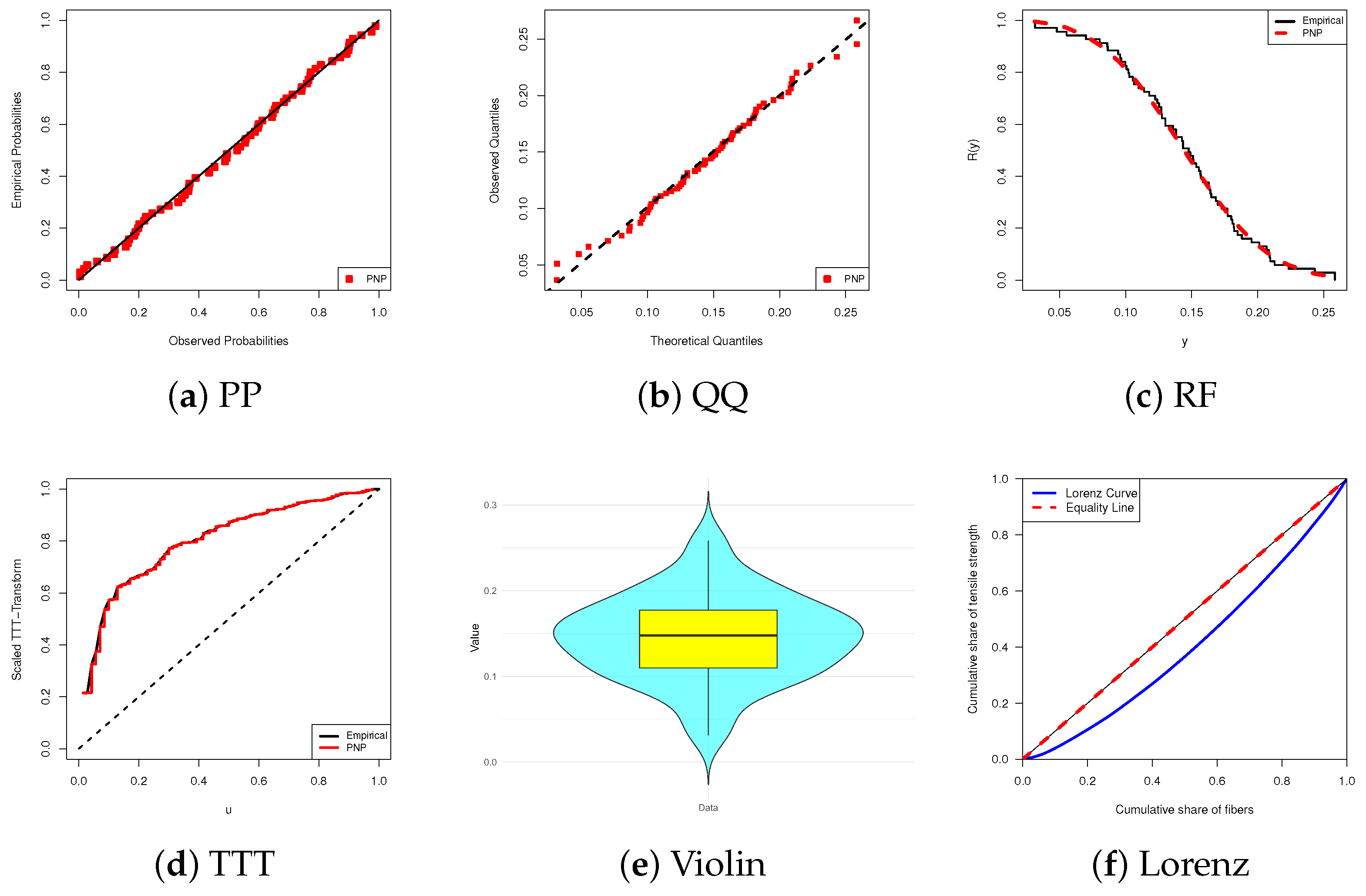
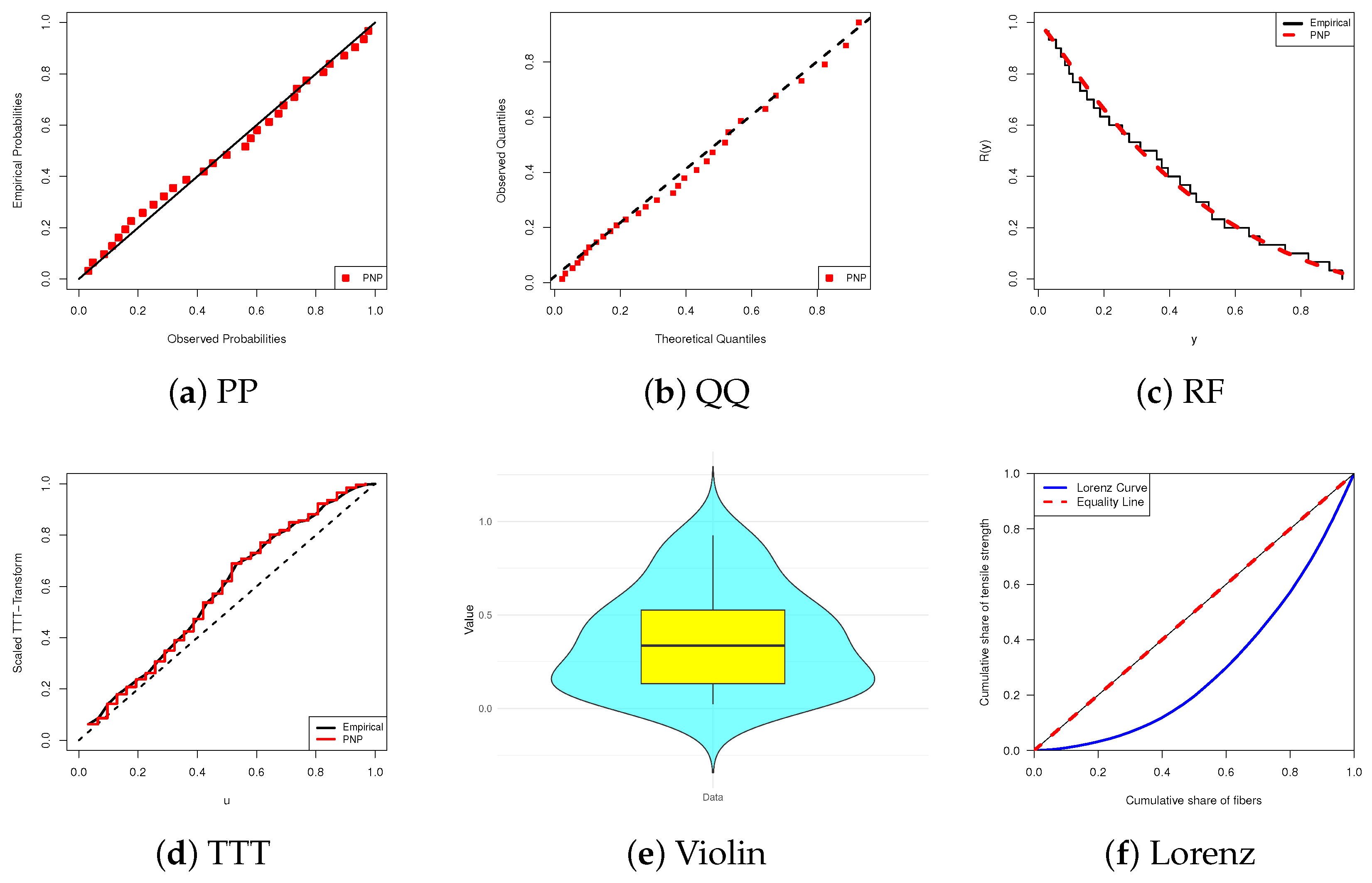
Before proceeding with the theoretical computations of the parameters a, b, c, R ( x ) , and h ( x ) outlined in earlier sections, we first illustrate the flexibility and efficacy of the proposed PNP lifetime model by examining its goodness-of-fit to the CF-TS dataset. Specifically, we calculate the Kolmogorov–Smirnov ( K S ) statistic along with its associated P-value. Using the AdequacyModel package developed by Marinho et al. [20], the MLEs of a, b, and c with their respective standard errors (Std.Errs) are obtained as 21.989(173.32), 3.3372(0.8584), and 19.463(196.54), respectively. The corresponding K S statistic and P-value are 0.0418 and 0.9997. Since the P-value substantially exceeds the preassigned significance level μ = 5 % , it can be concluded that the PNP model adequately represents the CF-TS data. To reinforce this assessment, Figure 9 provides a detailed visual evaluation through five diagnostic tools: (i) fitted versus empirical probability–probability (PP) plot, (ii) fitted versus empirical quantile–quantile (QQ) plot, (iii) fitted versus empirical RF, (iv) scaled total-time-on-test (TTT) transform, and (v) violin-boxplot.
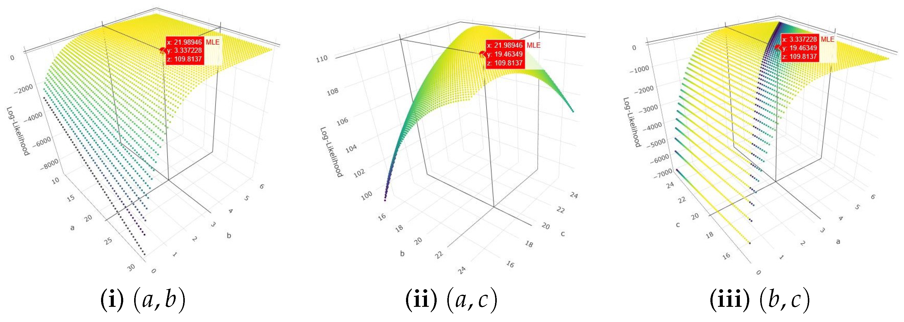
Subplots in Figure 9a–c corroborate the numerical results and further indicate that the PNP lifetime model provides an excellent fit to the CF-TS dataset. The TTT plot in Figure 9d demonstrates that the model closely follows the empirical curve, highlighting its capability to capture the observed increasing failure rate accurately. Figure 9e reveals that the CF-TS datasets appear moderately symmetric with a clear central concentration around the median and relatively low dispersion, indicating stable variability with no pronounced skewness or extreme tails. Figure 9f reveals that the Lorenz curve lies below the line of equality, meaning not all carbon fibers contribute equally to tensile strength. Low inequality (Gini ≈ 0.19) indicates that most carbon fibers have relatively similar tensile strengths, though some variation exists. Moreover, the 3D contour plots in Figure 10 confirm the existence and uniqueness of the MLEs for a, b, and c, providing additional evidence of the model’s stability and identifiability. The estimated values a ^ , b ^ , and c ^ can thus serve as robust initial values for subsequent analyses using this dataset.
Briefly, to see the effectiveness of the PNP distribution across the full CF-TS data, we compared it against bounded lifetime models (see Table 12). The model comparison was conducted using six widely used goodness-of-fit and information criteria:
(i)
log-likelihood ( L L );
(ii)
Akaike information criterion ( A I C );
(iii)
Bayesian information criterion ( B I C );
(vi)
Anderson–Darling ( A D );
(v)
Cramér–von Mises ( C v M );
(vi)
K S statistic along with its corresponding P-value.
Using the AdequacyModel package, the MLEs, together with their Std.Errs, in addition to the detailed results of criteria (i)–(vi), were calculated and summarized in Table 13. According to these model selection criteria, the best (optimal) model corresponds to the smallest values of A I C , B I C , A D , C v M , and K S , as well as the highest associated P-value. The comparative findings reported in Table 13 clearly demonstrate that the proposed PNP distribution provides the most competitive fit among all considered alternative bounded lifetime models listed in Table 12. These results strongly support the flexibility and practical effectiveness of the PNP model for modeling the CF-TS dataset.
To assess the theoretical outcomes of the PNP model parameters (a, b, c, R ( x ) , and h ( x ) at x = 0.1 ) alongside the BB distribution parameters ( π i , i = 1 , 2 ), the full CF-TS dataset was analyzed under a simultaneous life-testing experiment. The data were randomly divided into n = 20 groups, each consisting of s = 3 units, as presented in Table 14, where the marked values ‘✓’ indicate the first failure within each group. By setting π i = 1 for i = 1 , 2 and varying the number of failed units m, two datasets were constructed under the BB-PFF-CS framework (see Table 15).
In the absence of prior information regarding the PNP( α ) and BB( π ) parameters, a noninformative joint G-Sh.LN prior was adopted with hyperparameters G a m m a ( ϵ i , ε i ) = 0.001 for i = 1 , 2 and N ( μ , σ ) = ( 0.001 , 0.001 ) . The MCMC procedure described in Algorithm 1 was executed for = 30,000 iterations, discarding the initial = 5000 iterations as burn-in to ensure convergence.
Posterior summaries, including MCMC estimates and 95% BCI and HPD bounds, were obtained for a, b, c, R ( x ) , h ( x ) , and π i , i = 1 , 2 . Point estimates with their Std.Errs, as well as 95% interval estimates with their interval lengths, are reported in Table 16. Compared with classical LF-based estimates, the results in Table 16 indicate that the Bayesian approach exhibited improved performance, producing smaller Std.Errs for all parameters. Furthermore, the BCI and HPD intervals provided more precise inference than the asymptotic intervals (NA-ACI and NT-ACI), as reflected by their shorter ILs.
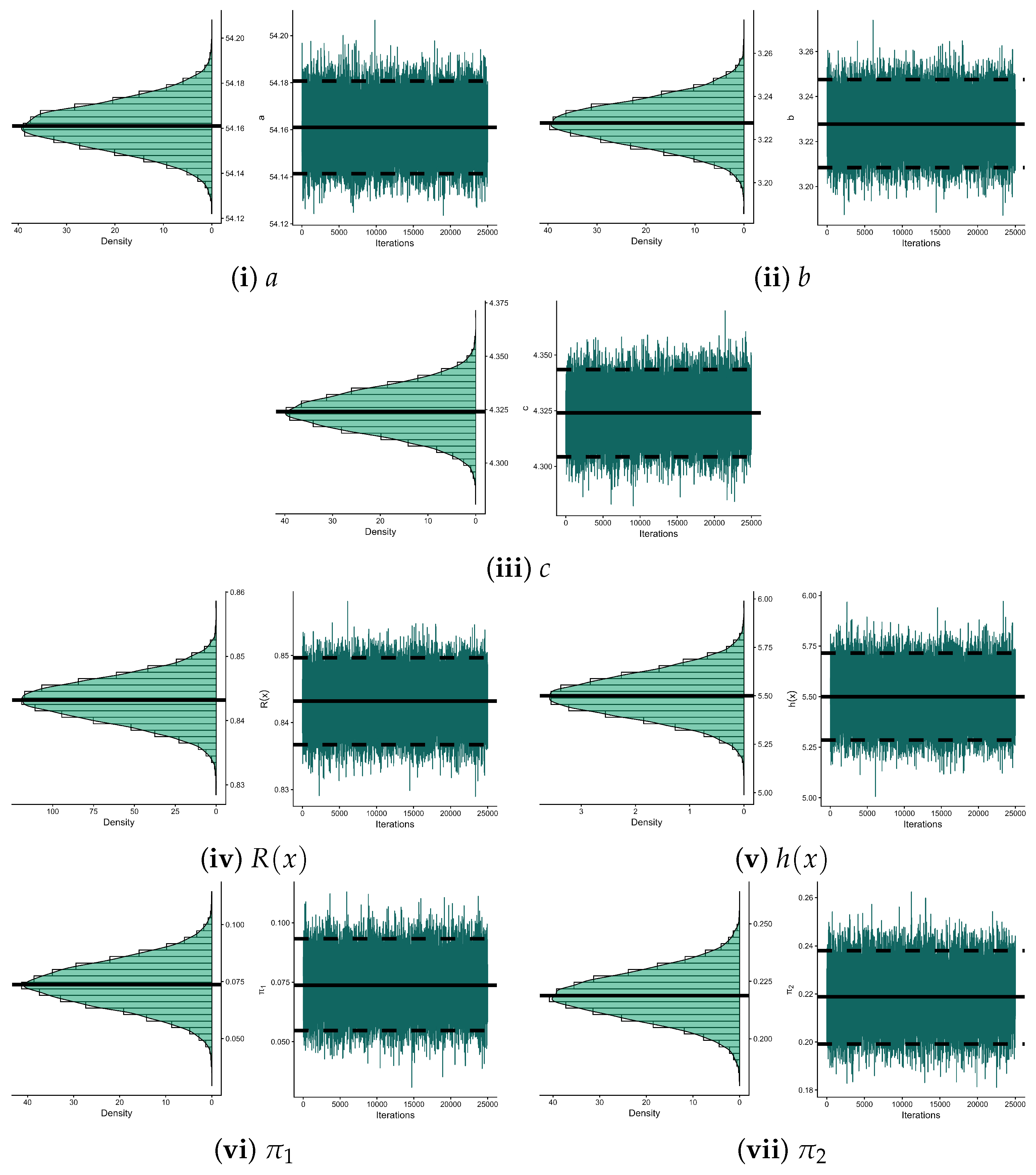
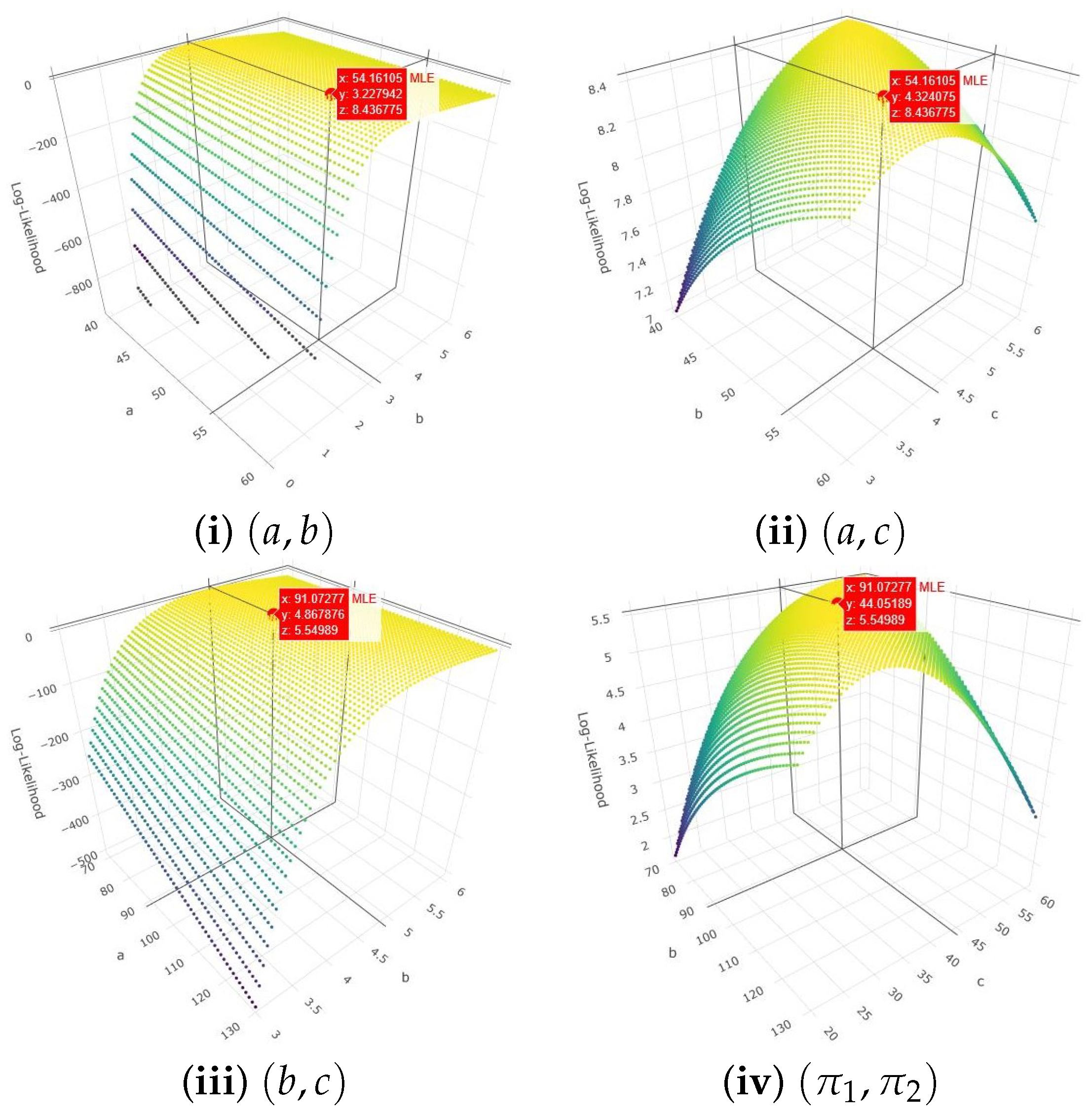
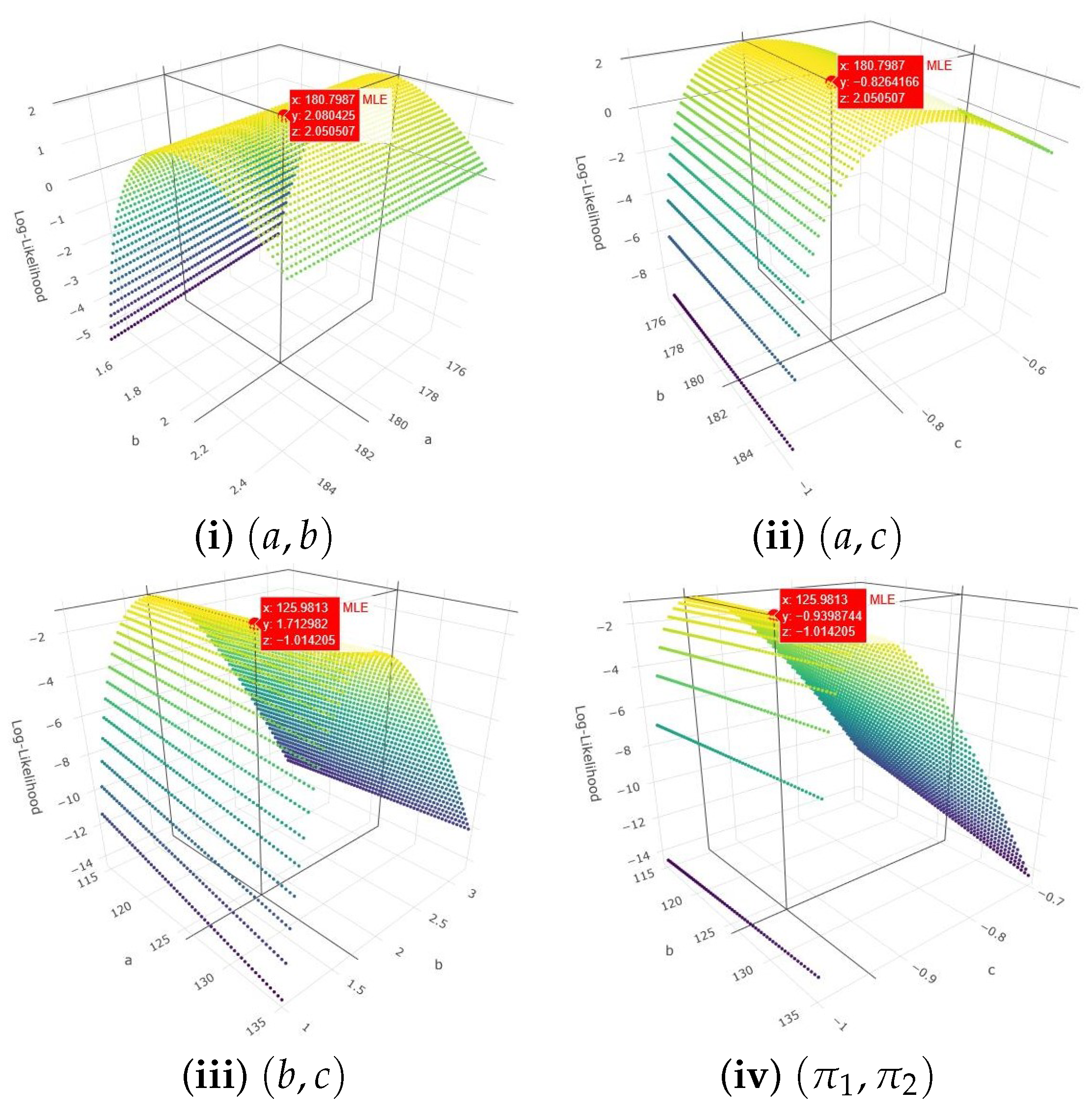
The facts shown in Figure 11 provide clear evidence regarding the behavior of the joint LF for the PNP ( α ) and BB ( π ) parameters. The 3D log-LF surfaces exhibit well-defined peaks, indicating that the MLEs reported in Table 16 not only exist but are also unique. For clarifications, both x- and y-axes represent the fitted estimates of a, b, c, or π i , i = 1 , 2 , while the z-axis represents the fitted log-LF value. This well-behaved structure reflects a stable estimation framework and supports the identifiability of the model parameters. Building on these findings, the MCMC-based inference further demonstrates strong computational reliability. To assess the convergence behavior of the simulated 25,000 Markov variates of a, b, c, R ( x ) , h ( x ) , and π i , i = 1 , 2 , we consider the BB-PFF-CS dataset at (2,10,35) with BB(0.5,0.5) (as a representative case) from Table 15.
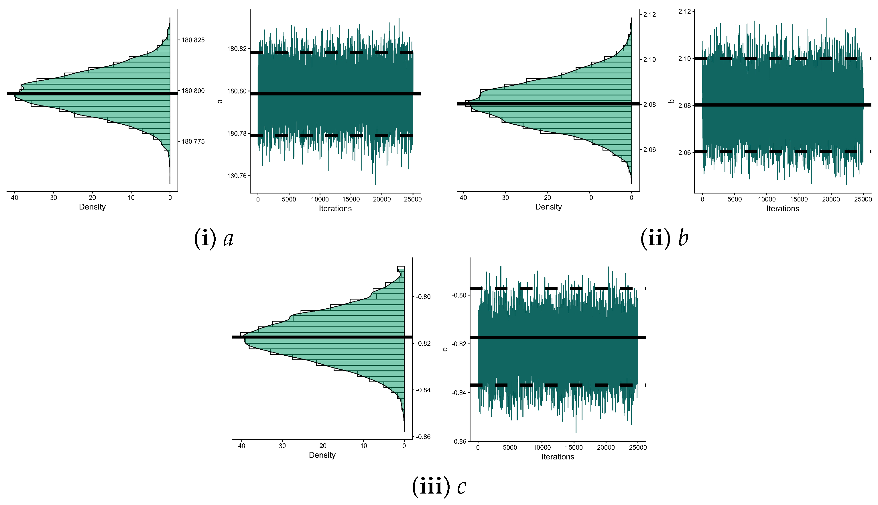
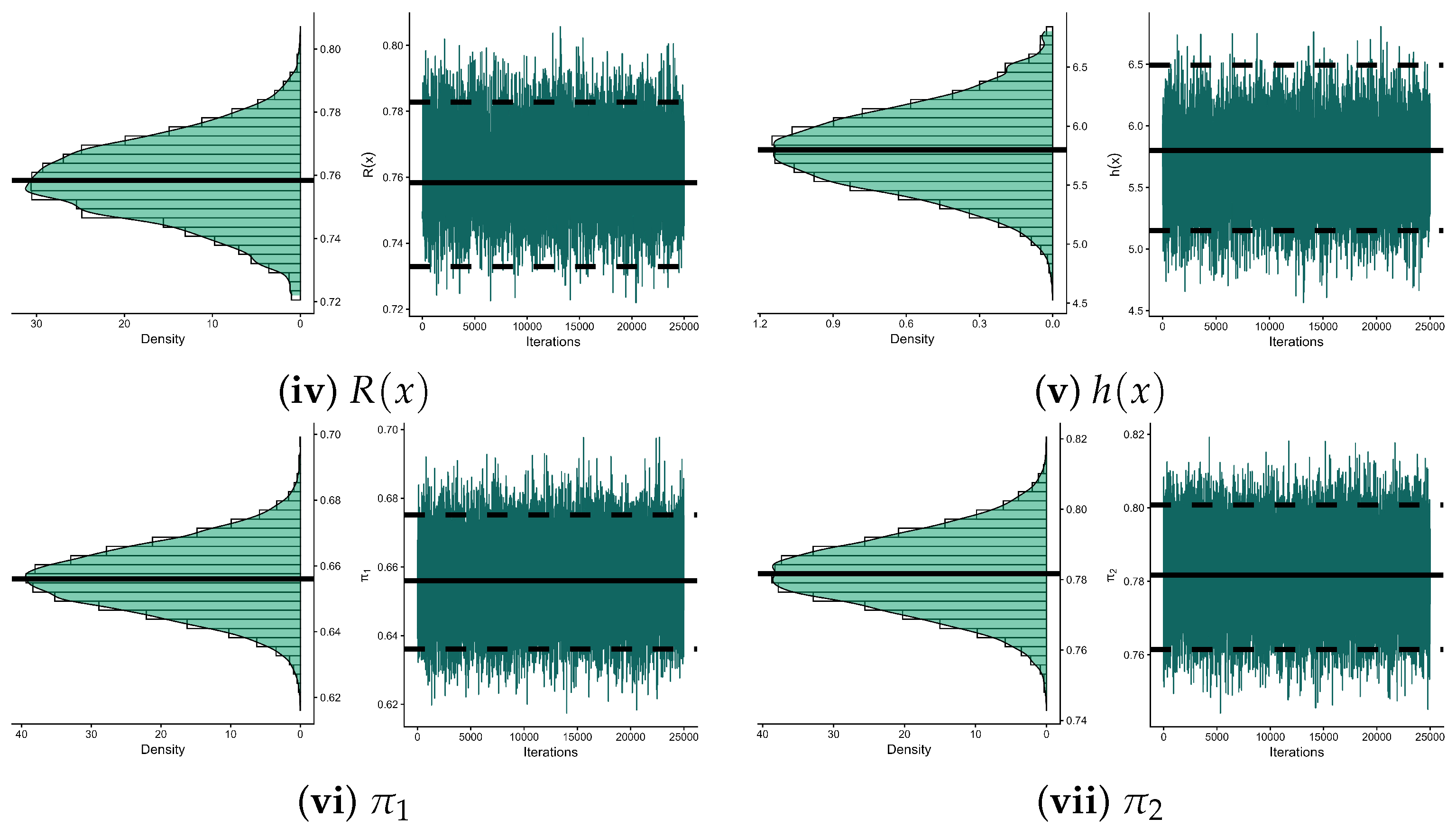
The frequency and trace diagrams of a, b, c, R ( x ) , h ( x ) , and π i , i = 1 , 2 shown in Figure 12 reveal that the simulated chains for all parameters fluctuate around constant levels without visible trends or drifts, suggesting rapid mixing and satisfactory convergence. The corresponding posterior density plots of a, b, c, R ( x ) , h ( x ) , and π i , i = 1 , 2 appear approximately symmetric and unimodal, reinforcing the stability of the estimation process. Moreover, the numerical summaries in Table 17, including quartiles, posterior means, modes, standard deviations (SDs), and skewness measures, are fully consistent with the graphical diagnostics. The relatively small dispersion and limited skewness observed across parameters confirm that the posterior distributions are well-concentrated and free from irregular behavior. Collectively, these results provide strong evidence that the proposed estimation procedure yields reliable, stable, and efficient inference for all model parameters under the BB-PFF-CS framework.

6.2. Polyester Fiber

Polyester fiber is a fundamental mechanical property that governs the performance, durability, and structural reliability of fiber-based products across numerous fields due to its high tensile strength, durability, and resistance to environmental effects. In the textile industry, it is a primary material for clothing, upholstery, carpets, and industrial fabrics. In engineering and industrial applications, polyester fibers are utilized in ropes, conveyor belts, tire cords, and reinforced composites. Additionally, in the medical and biomedical fields, polyester-based materials are used in surgical sutures, vascular grafts, and implants, owing to their stability and biocompatibility. In this application, we examine a genuine dataset comprising thirty failure records of polyester fiber tensile strength (PFTS); see Table 18. This dataset was evaluated using a universal testing machine with a standard design, ASTM D2256/D2256M-10; see Mazucheli et al. [28] and Mohammed et al. [29].
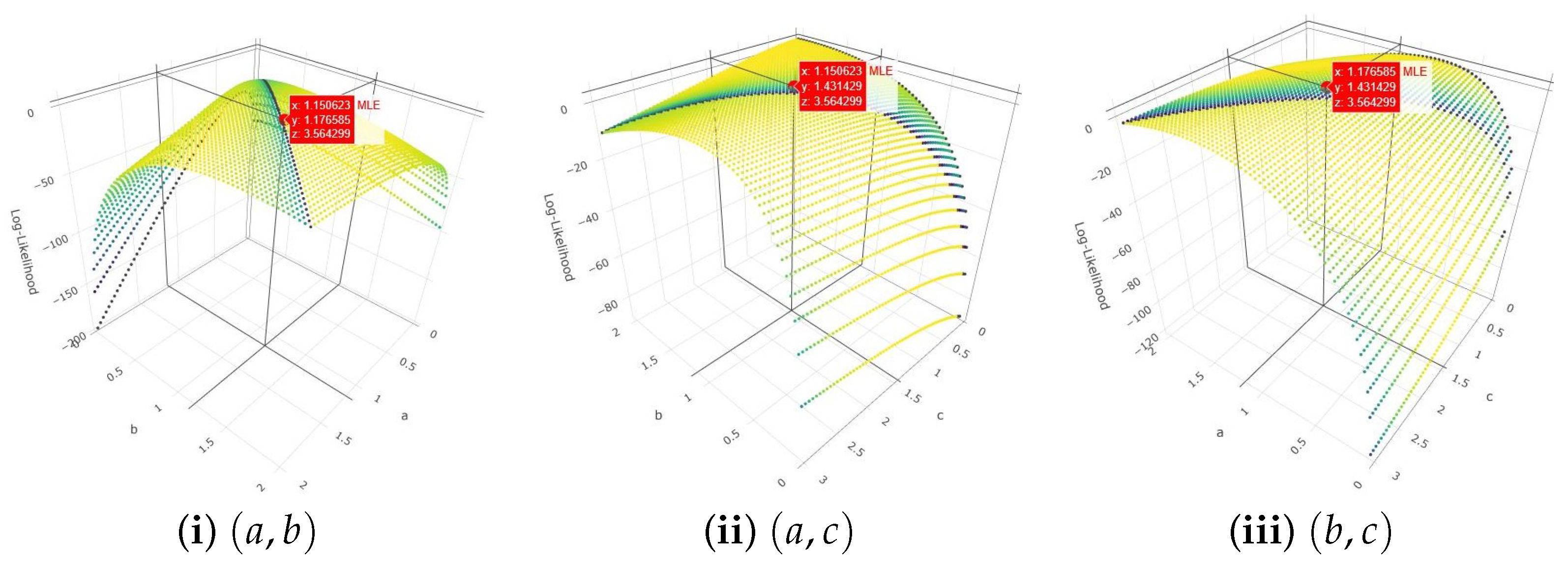
From Table 18, the fitted results for the MLE(Std.Err) of a, b, and c are 1.1506(0.5835), 1.1766(0.3759), and 1.4314(3.0662), respectively, while the corresponding K S (p-value) statistic is 0.0621(0.9993). Since the P-value is substantially higher than μ = 5 % , there is insufficient evidence to reject the null hypothesis, indicating that the PNP lifetime distribution provides an adequate fit to the PF-TS dataset. Figure 13a–c offer a complementary visual assessment, collectively reinforcing the numerical results and suggesting that the PNP model is highly suitable for capturing the characteristics of the entire PF-TS dataset. The TTT plot in Figure 13d closely tracks the empirical pattern, highlighting the model’s capacity to represent the increasing failure rate behavior observed in the data. The PF-TS data distribution shown in Figure 13e shows greater spread and a noticeable right-skew, with a longer upper tail, suggesting higher variability and the presence of larger values influencing the distribution. Figure 13f shows that the Lorenz curve lies far below the line of equality, indicating a higher degree of inequality in the tensile strengths of the fibers. A moderate Gini coefficient (Gini ≈ 0.41) suggests that the polyester fiber bundle is less homogeneous, with a notable variation among individual fiber strengths. Furthermore, the contour map in Figure 14 confirms the existence and uniqueness of the fitted MLEs a ^ , b ^ , and c ^ , demonstrating the model’s identifiability and numerical stability. Accordingly, the estimates a ^ 1.1506 , b ^ 1.1766 , and c ^ 1.4314 can be recommended as robust initial values for subsequent analytical procedures.
Again, to further assess the superiority of the proposed PNP distribution relative to other existing bounded lifetime models (listed in Table 12) across the full PF-TS dataset, Table 19 presents the fitting results for the PNP model alongside its competitors using the same goodness-of-fit and information criteria described in Section 6.1. The comparative findings reported in Table 19 indicate that the proposed PNP distribution consistently outperformed the competing models in terms of achieving the most favorable values for L L , A D , C v M , and K S statistics, as well as the largest corresponding p-value.
These results demonstrate the strong overall goodness-of-fit and distributional adequacy of the PNP model for the PF-TS dataset. Although the UW model, followed by the UG model, exhibited slightly better performance in terms of A I C and B I C statistics among the considered alternatives. Overall, these findings provide substantial empirical evidence supporting the robustness, adaptability, and superior fitting capability of the proposed PNP distribution for modeling PF-TS data.
To evaluate the theoretical estimators of the PNP model parameters (a, b, c, R ( x ) , and h ( x ) at x = 0.1 ) as well as the BB distribution parameters ( π i , i = 1 , 2 ), the complete PF-TS dataset was subjected to a simultaneous life-testing experiment and randomly partitioned into n = 10 groups, each containing s = 3 units (see Table 20). Using π i = 0.5 and 1 for i = 1 , 2 , multiple artificial BB-PFF-CS datasets were generated, as summarized in Table 21. In the absence of prior information on the PNP and BB model parameters, an improper G-Sh.LN prior was employed for a, b, and c. The MCMC procedure described in Algorithm 1 was implemented with = 30,000 iterations, discarding the first = 5000 iterations as burn-in to ensure convergence. The resulting theoretical estimates of a, b, c, R ( x ) , and h ( x ) obtained via the proposed methodology are presented in Table 22. As summarized in Table 22, the Bayesian estimates consistently yield smaller standard errors and narrower interval estimates compared with classical likelihood-based methods, highlighting improved precision and reliability. The consistency and stability of the estimates further confirm the suitability of the PNP and BB-PFF-CS frameworks for analyzing grouped lifetime data in practical engineering and material-strength studies.
To verify the existence and uniqueness of the MLEs for the parameters of PNP ( α ) and BB ( π ) , we utilize the datasets reported in Table 21. The three-dimensional log-LF surfaces displayed in Figure 15 for the parameters a, b, c, and π i , i = 1 , 2 , provide clear evidence that the estimated MLEs (listed in Table 22) for both PNP ( a , b ) and BB ( π 1 , π 2 ) not only exist but are also unique. These estimates are subsequently adopted as initial values for implementing the proposed MCMC procedures. To examine convergence, we analyze 25,000 simulated Markov chain samples for a, b, c, R ( x ) , h ( x ) , and π i , i = 1 , 2 , based on the BB-PFF-CS scheme with censoring configuration ( s , m , n ) = ( 2 , 5 , 10 ) and BB ( 0.5 , 0.5 ) , selected as a representative scenario from Table 21. The trace plots and posterior density estimates shown in Figure 16 illustrate the sampling behavior for each parameter. In these plots, the solid horizontal line indicates the posterior mean, whereas the dashed lines correspond to the 95 % Bayesian credible intervals. The trace plots exhibit stable and well-mixed patterns, suggesting satisfactory convergence of all chains. Further support is obtained from the summary statistics computed using the 30,000 post-burn-in samples. Specifically, the quartiles Q i , i = 1 , 2 , 3 , along with the posterior mean, mode, standard deviation, and skewness for each parameter, are reported in Table 23. These numerical results are consistent with the graphical diagnostics, confirming both convergence and distributional stability of the posterior samples across all parameters under study.

7. Conclusions, Limitations, and Future Research Directions

This study developed a comprehensive and unified reliability framework by integrating the BB-PFF-CS via a PNP-based distribution, introducing a flexible stochastic removal mechanism that overcomes the restrictive assumptions of conventional fixed-censoring schemes. The primary contribution lies in the formulation of a novel joint likelihood with a separable structure, which enables efficient and independent estimation of lifetime and removal parameters. In addition, both classical and Bayesian inferential procedures were systematically constructed, including MLE, NA-ACI, and NT-ACI, alongside a fully Bayesian approach based on a joint G-Sh.LN prior.
The implementation of an MH-MCMC algorithm further allowed reliable posterior inference despite analytical intractability. The proposed model demonstrated strong performance through simulation studies, sensitivity analyses, and real data applications, confirming its flexibility and effectiveness in modeling complex reliability behaviors.
From the numerical results, we now elucidate how the practical implications of the BB-PFF-CS–based framework translate into more reliable decision-making in engineering applications where testing resources are constrained, and censoring is unavoidable, as follows:
  • The consistent gains in estimation accuracy under the proposed framework demonstrate that explicitly modeling stochastic group removals can markedly improve inferential reliability when withdrawals are inherently uncertain. This is especially pertinent in practical settings, where equipment constraints, environmental variability, and operational disruptions often preclude strictly pre-specified censoring schemes.
  • From an engineering perspective, more precise parameter estimation translates directly into more accurate evaluation of reliability functions and hazard rates. These measures are fundamental for lifetime prediction, maintenance scheduling, and safety assessment, particularly in high-cost testing scenarios where complete lifetime data are often unattainable.
  • The simulation results further indicate that adopting a BB removal mechanism enhances adaptability across a wide range of experimental conditions. Such flexibility is crucial in modern materials testing, biomedical reliability studies, and industrial quality control, where random censoring patterns frequently arise.
  • The Gaussian proposal structure used within the MH algorithm contributed to stable posterior sampling and improved estimation efficiency, leading to comparatively smaller posterior standard errors and shorter interval estimates relative to the corresponding frequentist procedures.
  • In material strength applications, particularly for carbon and polyester fibers, the model captures realistic failure mechanisms where environmental conditions and specimen damage induce uncertainty in group removals during testing. In such experiments, it is common that not all remaining specimens are removed in a deterministic manner; instead, additional group removals may occur unpredictably due to equipment constraints, specimen fragility, or environmental conditions such as humidity and temperature fluctuations. The BB-PFF-CS mechanism adopted in this work captures this type of uncertainty more realistically than fixed or binomial-based censoring schemes.
  • In contrast, the proposed model provides engineers with a more flexible tool for quantifying material reliability under realistic testing conditions. The improved estimation accuracy of reliability and hazard functions can be used to better predict failure probabilities of composite materials, optimize safety margins in structural design, and support maintenance planning in industrial applications. Moreover, the Bayesian framework allows incorporating prior engineering knowledge when available, which is particularly useful in industrial settings where historical test data or expert judgment may be partially available.
  • Overall, these findings confirm that the proposed methodology is not only statistically robust but also practically meaningful, offering reliability engineers and applied researchers a more realistic and effective framework for analyzing bounded lifetime data under uncertain censoring environments.
An important avenue for future work is extending the BB-PFF-CS framework to multivariate reliability settings, which introduces both modeling and computational complexities. Defining dependence among multiple PNP lifetimes is challenging and may require copula-based or latent frailty approaches, while progressive censoring can exacerbate identifiability issues. On the computational side, higher-dimensional parameter spaces lead to more intricate posterior structures and slower MCMC convergence, necessitating advanced sampling techniques such as block updating or adaptive methods. Although the separable structure simplifies inference through conditional independence, it may limit the ability to capture realistic dependence between components. Therefore, future research should focus on partially separable or copula-enhanced models that balance flexibility with computational feasibility.
These limitations suggest several directions for future research. The framework can be extended to more general lifetime distributions or multi-parameter families to further enhance modeling flexibility. Incorporating covariates through regression-based extensions would allow for deeper insights into external effects on failure mechanisms. Exploring alternative stochastic removal schemes, such as negative binomial or zero-inflated models, may better capture different uncertainty patterns. From a computational standpoint, more efficient sampling techniques, including Hamiltonian Monte Carlo or variational Bayesian methods, could improve scalability and convergence. Extensions to multivariate and competing risks settings, as well as integration with accelerated life testing models, also represent important avenues for further development. Finally, additional validation using larger and more diverse datasets would strengthen the empirical generalizability of the proposed approach.


Author Contributions

Methodology, M.E.A.E., O.E.A.-K., S.A. and A.E.; Funding acquisition, M.E.A.E.; Software, A.E.; Resources, S.A.; Data curation, O.E.A.-K., Writing—original draft, M.E.A.E., S.A. and A.E.; Writing—review & editing, M.E.A.E., O.E.A.-K. and A.E. All authors have read and agreed to the published version of the manuscript.

Funding

The authors extend their appreciation to the Deanship of Scientific Research and Libraries in Princess Nourah bint Abdulrahman University for funding this research work through the Supporting Publication in Top-Impact Journals Initiative (SPTIF-2026).

Data Availability Statement

The authors confirm that the data supporting the findings of this study are available within the article.

Conflicts of Interest

The authors declare no conflicts of interest.

Appendix A. Delta Components of R(x) and h(x)

This appendix provides the required delta components to establish the approximate variances of R ( x ) and h ( x ) . The delta items in Σ R = ( Σ R a Σ R b Σ R c ) | ( α ^ = α ) and Σ h = ( Σ h a Σ h b Σ h c ) | ( α ^ = α ) are:
Σ R a = R ( x ) log R ( x ) 1 a ,
Σ R b = a x b log ( x ) R ( x ) 1 1 x b + c c x b + 1 ,
Σ R c = a x b R ( x ) c x b + 1 ,
Σ h a = 1 a h ( x ) ,
Σ h b = h ( x ) 1 b + log ( x ) x b log ( x ) 1 x b c x b log ( x ) c x b + 1 ,
and
Σ h c = a b x b 1 ( 1 x b ) ( c x b + 1 ) 1 ( c + 1 ) x b ( c x b + 1 ) .

References

  1. Karakaya, K.; Rajitha, C.S.; Sağlam, Ş.; Tashk, Y.A.; Bakr, M.E.; Muse, A.H.; Kumar, A.; Hussam, E.; Gemeay, A.M. A new unit distribution: Properties, estimation, and regression analysis. Sci. Rep. 2024, 14, 7214. [Google Scholar] [CrossRef] [Scilit] [PubMed]
  2. Wu, J.W.; Hung, W.L.; Chen, C.Y. Approximate MLE of the scale parameter of the truncated Rayleigh distribution under the first failure-censored data. J. Inf. Optim. Sci. 2004, 25, 221–235. [Google Scholar] [CrossRef] [Scilit]
  3. Balasooriya, U. Failure–censored reliability sampling plans for the exponential distribution. J. Stat. Comput. Simul. 1995, 52, 337–349. [Google Scholar] [CrossRef] [Scilit]
  4. Balakrishnan, N.; Cramer, E. The Art of Progressive Censoring. In Statistics for Industry and Technology; Birkhäuser: New York, NY, USA, 2014. [Google Scholar]
  5. Huang, S.R.; Wu, S.J. Estimation of Pareto distribution under progressive first-failure censoring with random removals. J. Chin. Stat. Assoc. 2011, 49, 82–97. [Google Scholar]
  6. Ashour, S.K.; El-Sheikh, A.A.; Elshahhat, A. Inferences for Weibull parameters under progressively first-failure censored data with binomial random removals. Stat. Optim. Inf. Comput. 2021, 9, 47–60. [Google Scholar] [CrossRef] [Scilit]
  7. Singh, S.K.; Singh, U.; Sharma, V.K. Expected total test time and Bayesian estimation for generalized Lindley distribution under progressively Type-II censored sample where removals follow the beta-binomial probability law. Appl. Math. Comput. 2013, 222, 402–419. [Google Scholar] [CrossRef] [Scilit]
  8. Elshahhat, A.; Sharma, V.K.; Mohammed, H.S. Statistical analysis of progressively first-failure-censored data via beta-binomial removals. AIMS Math. 2023, 8, 22419–22446. [Google Scholar] [CrossRef] [Scilit]
  9. Lawless, J.F. Statistical Models and Methods for Lifetime Data; John Wiley and Sons: Manhattan, NY, USA, 2011. [Google Scholar]
  10. Greene, W.H. Econometric Analysis, 4th ed.; Prentice-Hall: New York, NY, USA, 2000. [Google Scholar]
  11. Meeker, W.Q.; Escobar, L.A. Statistical Methods for Reliability Data; John Wiley and Sons: Manhattan, NY, USA, 2014. [Google Scholar]
  12. Bernardo, J.M.; Smith, A.F.; Berliner, M. Bayesian Theory; Wiley: Manhattan, NY, USA, 1994. [Google Scholar]
  13. Gelman, A.; Carlin, J.B.; Stern, H.S.; Dunson, D.B.; Vehtari, A.; Rubin, D.B. Bayesian Data Analysis, 3rd ed.; Chapman and Hall/CRC: Boca Raton, FL, USA, 2013. [Google Scholar]
  14. Henningsen, A.; Toomet, O. maxLik: A package for maximum likelihood estimation in R. Comput. Stat. 2011, 26, 443–458. [Google Scholar] [CrossRef] [Scilit]
  15. Plummer, M.; Best, N.; Cowles, K.; Vines, K. coda: Convergence diagnosis and output analysis for MCMC. R News 2006, 6, 7–11. [Google Scholar]
  16. Kundu, D. Bayesian inference and life testing plan for the Weibull distribution in presence of progressive censoring. Technometrics 2008, 50, 144–154. [Google Scholar] [CrossRef] [Scilit]
  17. Singh, S.V.; Sharma, V.K.; Singh, S.K. Inferences for two parameter Teissier distribution in case of fuzzy progressively censored data. Reliab. Theory Appl. 2022, 17, 559–573. [Google Scholar]
  18. Nassar, M.; Alotaibi, R.; Elshahhat, A. Bayesian estimation of some reliability characteristics for Nakagami model using adaptive progressive censoring. Phys. Scr. 2024, 99, 095271. [Google Scholar] [CrossRef] [Scilit]
  19. Ahmad, H.H.; Abo-Kasem, O.E.; Rabaiah, A.; Elshahhat, A. Survival analysis of newly extended Weibull data via adaptive progressive Type-II censoring and its modeling to Carbon fiber and electromigration. AIMS Math. 2025, 10, 10228–10262. [Google Scholar] [CrossRef] [Scilit]
  20. Marinho, P.R.D.; Silva, R.B.; Bourguignon, M.; Cordeiro, G.M.; Nadarajah, S. AdequacyModel: An R package for probability distributions and general purpose optimization. PLoS ONE 2019, 14, e0221487. [Google Scholar] [CrossRef] [Scilit] [PubMed]
  21. Althubyani, F.A.; Abd El-Bar, A.M.T.; Fawzy, M.A.; Gemeay, A.M. A new 3-parameter bounded beta distribution: Properties, estimation, and applications. Axioms 2022, 11, 504. [Google Scholar] [CrossRef] [Scilit]
  22. Guerra, R.R.; Peña-Ramírez, F.A.; Bourguignon, M. The unit extended Weibull families of distributions and its applications. J. Appl. Stat. 2021, 48, 3174–3192. [Google Scholar] [CrossRef] [Scilit]
  23. Mazucheli, J.; Menezes, A.F.B.; Ghitany, M.E. The unit-Weibull distribution and associated inference. J. Appl. Probab. Stat. 2018, 13, 1–22. [Google Scholar]
  24. Dey, S.; Menezes, A.F.; Mazucheli, J. Comparison of estimation methods for unit-gamma distribution. J. Data Sci. 2019, 17, 768–801. [Google Scholar] [CrossRef] [Scilit]
  25. Mazucheli, J.; Menezes, A.F.; Dey, S. The unit-Birnbaum-Saunders distribution with applications. Chil. J. Stat. 2018, 9, 47–57. [Google Scholar]
  26. Kumaraswamy, P. A generalized probability density function for double-bounded random processes. J. Hydrol. 1980, 46, 79–88. [Google Scholar] [CrossRef] [Scilit]
  27. Gupta, A.K.; Nadarajah, S. Handbook of Beta Distribution and Its Applications; CRC Press: Boca Raton, FL, USA, 2004. [Google Scholar]
  28. Mazucheli, J.; Menezes, A.F.; Dey, S. Unit-Gompertz distribution with applications. Statistica 2019, 79, 25–43. [Google Scholar]
  29. Mohammed, H.S.; Abo-Kasem, O.E.; Elshahhat, A. Optimum Analysis and Parameter Inference of a New Improved Adaptive Progressive Unit-Weibull Model Censoring with Two Physical Applications. Rev. Int. Métodos Numér. Para Cálculo Diseño Ing. 2025, 41, 8. [Google Scholar] [CrossRef] [Scilit]
Figure 1. Shapes of the PNP ( α ) distribution.
Mathematics 14 01803 g001
Figure 2. A flowchart of the proposed inference frameworks for the PNP-BB-PFF-CS framework.
Mathematics 14 01803 g002
Figure 3. Shapes for likelihood, prior, and posterior densities of ( a , b ) (top) and ( π 1 , π 2 ) (bottom).
Mathematics 14 01803 g003
Figure 4. Shapes for likelihood, prior, posterior densities of c.
Mathematics 14 01803 g004
Figure 5. Sensitivity maps of a, b, and c from Pop-i for i = 1 , 2 .
Mathematics 14 01803 g005
Figure 6. The BGR diagnostic from Pop-i for i = 1 , 2 .
Mathematics 14 01803 g006
Figure 7. The ACF (left), Ergodic (center), and Trace (right) convergence diagnostics for MCMC iterations of a, b, c, R ( x ) , and h ( x ) from Pop-1.
Mathematics 14 01803 g007
Figure 8. Prior robustness diagnostics for the PNP ( α ) model from Pop-1 (top) and Pop-2 (bottom).
Mathematics 14 01803 g008
Figure 9. Six visual fit tools for the PNP model from CF-TS data.
Mathematics 14 01803 g009
Figure 10. 3D contour diagrams of a, b, and c from CF-TS data.
Mathematics 14 01803 g010
Figure 11. Contours of PNP and BB parameters from CF-TS data.
Mathematics 14 01803 g011
Figure 12. Convergence diagnostics of PNP and BB parameters from CF-TS data.
Mathematics 14 01803 g012
Figure 13. Six visual fit tools for the PNP model from PF-TS data.
Mathematics 14 01803 g013
Figure 14. 3D contour diagrams of a, b, and c from PF-TS data.
Mathematics 14 01803 g014
Figure 15. Contours of PNP and BB parameters from PF-TS data.
Mathematics 14 01803 g015
Figure 16. Convergence diagnostics of PNP and BB parameters from PF-TS data.
Mathematics 14 01803 g016aMathematics 14 01803 g016b
Table 1. The RMSEs (1st Col.) and AABs (2nd Col.) of a.
(n, m)MLEMCMC [P1]MCMC [P2]MLEMCMC [P1]MCMC [P2]
Pop-1
( s , π 1 , π 2 ) (2,0.5,0.5)(5,0.5,0.5)
(20,10)1.21460.78240.39420.37780.24800.22421.26501.17080.39490.37900.25700.2329
(20,15)0.79420.54270.38430.36910.22560.19300.91150.75430.38710.36970.23830.1995
(50,20)0.48530.37570.37460.35810.19510.18230.73600.41510.37500.35970.20390.1928
(50,40)0.41390.34780.34020.23550.16900.13170.49470.34890.34130.24450.18380.1539
(80,30)0.36900.31300.29270.22760.14100.12500.41390.31590.29830.23670.15040.1322
(80,60)0.34870.27310.24050.22380.11220.09270.38840.28490.25480.23640.12080.1029
( s , π 1 , π 2 ) (2,1.5,1.5)(5,1.5,1.5)
(20,10)1.31621.11380.51510.42020.35290.31691.38051.19750.51750.42070.35550.3206
(20,15)1.02190.58040.38700.37690.23240.21971.16090.99200.38840.37780.24220.2251
(50,20)0.58210.38180.37770.36410.19790.18860.89360.41940.37830.36490.20560.1977
(50,40)0.43950.35670.35030.23800.17680.16200.55240.35840.35250.24670.18780.1726
(80,30)0.39080.33270.31640.22760.14780.12750.43920.33980.31970.23730.15780.1367
(80,60)0.35900.29070.28390.22560.12070.09360.39120.29930.28870.23660.13730.1179
Pop-2
( s , π 1 , π 2 ) (2,0.5,0.5)(5,0.5,0.5)
(20,10)2.02231.11630.94600.93760.68260.55182.14081.60801.05070.94110.69780.5710
(20,15)1.89171.05480.89340.69120.52360.42761.98551.56830.92900.88950.55810.4636
(50,20)1.72220.96220.83050.58020.41210.34661.78561.14900.92640.82470.45400.3921
(50,40)1.60620.90950.78530.45630.32510.28341.75120.92490.84000.77230.36560.3047
(80,30)1.51730.87920.70150.32330.27680.23461.62970.90820.72030.61120.31510.2763
(80,60)1.00640.64720.45240.25490.19670.14291.10460.68910.50170.44710.22170.1746
( s , π 1 , π 2 ) (2,1.5,1.5)(5,1.5,1.5)
(20,10)2.13861.20071.11451.08820.70620.56432.22711.83631.17451.09090.71760.5779
(20,15)1.98491.08740.90410.73470.53170.49912.02961.57230.98310.89950.56550.5126
(50,20)1.84200.99540.87360.64500.47190.42371.89101.16700.92760.86710.53620.4600
(50,40)1.66280.92160.81520.57310.40990.33681.76840.93250.89590.80290.44070.3762
(80,30)1.56190.89710.76440.40720.32420.28091.69400.92340.77760.65040.34350.2867
(80,60)1.18420.86410.69890.30420.23400.14881.47560.88020.71380.60100.25400.1854
Table 2. The RMSEs (1st Col.) and AABs (2nd Col.) of b.
(n, m)MLEMCMC [P1]MCMC [P2]MLEMCMC [P1]MCMC [P2]
Pop-1
( s , π 1 , π 2 ) (2,0.5,0.5)(5,0.5,0.5)
(20,10)1.35111.15960.58490.47320.28990.24301.15520.88540.49770.45370.27540.2346
(20,15)0.94510.70940.43710.34060.27150.22830.91130.69210.39860.32290.25490.2184
(50,20)0.62570.48930.38110.30900.24260.19520.59610.45220.37080.28910.22100.1830
(50,40)0.51790.40490.37020.28420.21770.18420.50380.37920.33480.28360.21310.1791
(80,30)0.45640.34970.30960.24080.19590.16660.42780.32770.25530.20010.18920.1574
(80,60)0.41570.33230.24980.20410.16270.13800.41190.31910.22520.18560.15720.1281
( s , π 1 , π 2 ) (2,1.5,1.5)(5,1.5,1.5)
(20,10)1.54601.25800.74510.58030.31090.25971.26590.95880.72350.45440.29400.2500
(20,15)1.04270.76190.49770.45410.28910.23000.97980.74960.45720.34760.25880.2240
(50,20)0.85810.52870.38140.31790.24440.20420.61730.48530.37470.30990.23190.2029
(50,40)0.54950.44420.37180.29460.22690.18590.54370.42570.35550.28650.21710.1804
(80,30)0.46850.35920.33770.27750.20690.17350.44350.35030.33250.27020.19490.1637
(80,60)0.45230.34080.27590.22550.18420.14850.41390.32380.23500.19200.17640.1482
( s , π 1 , π 2 ) (2,0.5,0.5)(5,0.5,0.5)
(20,10)2.02621.13140.68380.65080.62220.39341.34251.12970.67780.64130.53820.3379
(20,15)1.47201.00110.54160.49960.42940.31971.26980.99840.50590.44410.37270.2903
(50,20)0.71450.49060.44620.40170.37810.30070.71430.48950.43440.39110.33370.2437
(50,40)0.64600.45180.37640.33950.30670.27190.64600.45170.37280.32520.28660.2243
(80,30)0.51130.40420.28020.23920.22410.19900.51080.40350.26120.23240.20900.1912
(80,60)0.45280.32360.25370.20600.17180.16900.45280.32360.23320.20590.16990.1413
( s , π 1 , π 2 ) (2,1.5,1.5)(5,1.5,1.5)
(20,10)1.69791.44370.79310.74560.68870.58331.82321.34860.76320.71040.65060.4989
(20,15)1.60771.27990.54720.51660.46270.35091.50101.11200.52730.50660.43800.3059
(50,20)0.82640.58570.45960.43490.38390.30710.81470.57510.43950.39700.33770.2814
(50,40)0.65050.47580.41540.39550.34630.27980.65050.47560.40680.37500.33040.2399
(80,30)0.63700.44090.33090.27770.24880.23550.63700.44080.29420.27330.23580.2066
(80,60)0.47290.36330.26290.23580.19960.18200.47260.36180.25530.22060.19700.1711
Table 3. The RMSEs (1st Col.) and AABs (2nd Col.) of c.
(n, m)MLEMCMC [P1]MCMC [P2]MLEMCMC [P1]MCMC [P2]
Pop-1
( s , π 1 , π 2 ) (2,0.5,0.5)(5,0.5,0.5)
(20,10)1.53741.01040.35540.28860.22560.20061.26540.90920.33600.27570.20250.1739
(20,15)1.46750.85240.26530.23270.21620.18951.04420.80620.26450.23260.19110.1550
(50,20)1.23100.78660.24900.21500.19130.16500.81930.71230.22840.19830.17810.1433
(50,40)1.05370.60290.21560.17870.17500.15190.71530.60190.20730.17570.15200.1236
(80,30)0.82800.51480.21270.17650.16060.13350.63340.51070.19050.16620.13970.1074
(80,60)0.69260.34180.18390.15430.14370.12260.50640.34170.17090.14810.13060.1054
( s , π 1 , π 2 ) (2,1.5,1.5)(5,1.5,1.5)
(20,10)1.65911.19400.47540.41010.26290.21601.30050.98610.42240.32660.24150.1922
(20,15)1.49580.91770.30460.26920.22540.19311.11980.89960.28700.24760.19770.1735
(50,20)1.37620.81960.26010.21790.20110.17840.96600.75220.24150.21440.18790.1547
(50,40)1.19390.64700.21910.18690.17580.15220.75260.64690.20890.18500.15780.1317
(80,30)0.88400.54540.21360.17810.16220.14540.69190.54490.19760.17520.14770.1234
(80,60)0.74180.34800.20360.17360.15050.12380.64120.34560.19010.16030.13270.1068
( s , π 1 , π 2 ) (2,0.5,0.5)(5,0.5,0.5)
(20,10)1.58311.21030.82320.78270.71240.66101.29530.94010.80400.74560.68350.5705
(20,15)1.47910.82500.71830.67230.58190.39281.14570.77590.70590.61160.55810.3173
(50,20)1.32560.78180.54850.47290.35240.29080.85140.61550.47790.40980.30610.2515
(50,40)1.08280.46930.37800.33410.29800.27400.67770.39900.36780.30190.28830.2450
(80,30)0.91920.38840.33640.28990.28900.24370.43700.35810.30050.28960.24960.2350
(80,60)0.67010.30690.25660.24750.21090.19340.40680.28100.25020.23940.19930.1837
( s , π 1 , π 2 ) (2,1.5,1.5)(5,1.5,1.5)
(20,10)1.71551.26590.95400.87090.72630.66951.38491.10340.92280.85170.69570.5774
(20,15)1.50390.91890.76330.73220.61840.59631.22420.82750.75400.72340.60120.5153
(50,20)1.41520.80700.59650.52180.46270.35850.97650.63150.52210.49410.41460.2976
(50,40)1.22950.56920.41250.34200.31560.28900.78360.47520.39740.33990.30530.2494
(80,30)0.96230.41800.36470.33330.29120.27260.49510.37590.33360.29700.27730.2405
(80,60)0.87370.35960.31070.26200.25400.22360.38950.33890.27970.26150.22420.2117
Table 4. The RMSEs (1st Col.) and AABs (2nd Col.) of R ( x ) .
(n, m)MLEMCMC [P1]MCMC [P2]MLEMCMC [P1]MCMC [P2]
Pop-1
( s , π 1 , π 2 ) (2,0.5,0.5)(5,0.5,0.5)
(20,10)0.33290.23340.22190.21580.18550.17530.43290.23390.22610.21790.19790.1820
(20,15)0.23920.22760.21840.18270.16590.15900.24000.22810.22230.19000.17500.1659
(50,20)0.22800.22200.21520.17290.15930.15460.22880.22260.21880.17680.16580.1561
(50,40)0.22530.21470.20630.15910.14510.12520.22600.21760.20890.16130.14690.1388
(80,30)0.21450.21210.20110.14630.13130.11050.21640.21400.20330.15530.14050.1259
(80,60)0.21350.19090.16480.13920.12230.10720.21570.19590.17290.15460.13680.1179
( s , π 1 , π 2 ) (2,1.5,1.5)(5,1.5,1.5)
(20,10)0.24630.23170.21900.19400.18250.16920.24650.23210.22310.19900.19160.1789
(20,15)0.23280.22480.21600.18180.16320.15540.23410.22580.22100.18880.17050.1614
(50,20)0.22640.22070.21500.16870.15240.13930.22720.22170.21830.17460.15570.1516
(50,40)0.22230.21430.20630.15620.13820.12370.22350.21720.20770.15830.14300.1356
(80,30)0.21370.19950.19660.14410.12260.11000.21630.20170.19860.15490.14040.1223
(80,60)0.21170.18600.16350.13870.09540.07920.21450.18960.17100.15230.11920.0922
( s , π 1 , π 2 ) (2,0.5,0.5)(5,0.5,0.5)
(20,10)0.34270.32350.31670.28850.27630.22000.36520.34250.33430.31220.27820.2744
(20,15)0.31300.30970.28320.27460.27150.20370.31420.31090.30840.27860.27320.2310
(50,20)0.30700.30350.26890.23190.21020.19160.30890.30510.27590.24010.21710.2075
(50,40)0.30080.29170.26660.20870.19980.18570.30190.29270.27460.21200.20340.1943
(80,30)0.29060.28350.26560.19030.17360.14820.29280.28530.27170.19840.18110.1626
(80,60)0.26990.26740.26390.18400.16420.11040.27410.26910.26440.19170.17450.1300
( s , π 1 , π 2 ) (2,1.5,1.5)(5,1.5,1.5)
(20,10)0.33370.32240.30700.27550.27270.21010.33440.32290.31410.28720.27400.2398
(20,15)0.30810.30540.27220.24330.22570.19610.31000.30660.27740.25730.23360.2237
(50,20)0.30580.29550.26750.22620.20770.18880.30800.29860.27510.23180.21420.2062
(50,40)0.29690.28920.26590.19530.18120.16650.29840.29060.27380.19910.18360.1738
(80,30)0.28090.27710.26470.18710.16500.12900.28310.28050.27040.19610.17520.1535
(80,60)0.26700.26520.26200.16670.10170.08020.26860.26560.26360.18550.10530.0866
Table 5. The RMSEs (1st Col.) and AABs (2nd Col.) of h ( x ) .
(n, m)MLEMCMC [P1]MCMC [P2]MLEMCMC [P1]MCMC [P2]
Pop-1
( s , π 1 , π 2 ) (2,0.5,0.5)(5,0.5,0.5)
(20,10)0.26130.24830.24360.20220.18500.18190.26370.24870.24700.20770.20140.1829
(20,15)0.25020.24190.23880.18730.17630.16610.25310.24250.24140.19850.18230.1697
(50,20)0.24480.24040.23750.16760.16400.15800.24520.24060.24010.17560.16690.1633
(50,40)0.24170.23720.22810.15550.13650.12400.24240.23840.22890.16450.14070.1271
(80,30)0.23630.22300.22120.15440.12890.11090.23760.22350.22150.16360.13340.1198
(80,60)0.23550.21570.19720.15180.09970.08250.23690.21720.20190.16180.11010.0979
( s , π 1 , π 2 ) (2,1.5,1.5)(5,1.5,1.5)
(20,10)0.29240.25460.24460.22080.20060.18310.31290.25500.24760.22340.20500.1980
(20,15)0.25750.24580.23940.19330.18200.16610.25820.24620.24250.19890.18300.1708
(50,20)0.24530.24160.23810.17650.16790.16450.24580.24120.24120.17790.16960.1657
(50,40)0.24270.23750.23420.16460.15850.15030.24360.24000.23530.16920.16100.1576
(80,30)0.23640.22380.22230.15530.13500.12330.23820.22600.22370.16380.13880.1243
(80,60)0.23620.21850.20190.15280.11880.10060.23760.22100.20400.16310.13070.1178
( s , π 1 , π 2 ) (2,0.5,0.5)(5,0.5,0.5)
(20,10)0.66110.63590.59420.58050.51940.41560.66280.63710.59490.59120.52800.4548
(20,15)0.61200.60210.56520.44870.42070.40350.61490.60430.57450.46060.44540.4113
(50,20)0.60350.58710.56220.41760.38780.37570.60770.59130.56810.41890.40710.3876
(50,40)0.59850.57840.56060.37700.32130.29560.60010.58070.56590.39910.35490.3206
(80,30)0.55990.55610.54790.37130.30460.26270.56260.55860.55370.39660.33430.2896
(80,60)0.55490.53550.53320.35600.19240.11180.55810.53800.53370.37590.21610.1449
( s , π 1 , π 2 ) (2,1.5,1.5)(5,1.5,1.5)
(20,10)0.68030.66340.60330.58200.53330.45690.68170.66440.60820.59580.54950.5301
(20,15)0.61700.61510.56860.46510.44600.40550.61880.61630.57910.49300.45330.4298
(50,20)0.60610.59680.56370.44460.41980.39370.60790.59940.56880.45310.42110.3970
(50,40)0.60310.58360.56150.40630.38050.34400.60760.58520.56620.40720.40010.3677
(80,30)0.57300.56920.55900.37630.31670.29530.57490.57230.56400.39790.34350.3116
(80,60)0.55570.54790.54420.36250.24460.19420.56010.54890.54440.38480.28890.2412
Table 6. The 95% interval estimation results of a.
(N, M)NA-ACINT-ACIBCI [P1]BCI [P2]HPD [P1]HPD [P2]
( s , π 1 , π 2 ) Pop-1→
(2,0.5,0.5)
(20,10)0.8860.9460.7920.9510.5490.9640.4170.9710.2680.9790.2140.982
(20,15)0.7960.9510.6940.9560.4590.9690.3330.9750.1800.9840.1670.984
(50,20)0.5420.9640.4010.9720.3050.9770.2950.9770.1360.9860.1270.986
(50,40)0.3280.9760.2630.9790.2260.9810.1310.9860.1110.9870.1000.988
(80,30)0.2880.9780.2350.9810.1900.9830.1150.9870.0940.9880.0900.988
(80,60)0.2180.9820.1880.9830.1650.9840.0870.9890.0800.9890.0780.989
(5,0.5,0.5)
(20,10)0.9800.9410.8210.9500.5760.9630.4400.9700.2860.9780.2170.982
(20,15)0.8490.9480.7190.9550.4600.9690.3370.9750.2100.9820.1760.984
(50,20)0.5680.9630.4620.9690.3080.9770.3000.9770.1370.9860.1280.986
(50,40)0.3360.9750.2780.9780.2260.9810.1400.9860.1210.9870.1030.988
(80,30)0.2940.9780.2380.9810.1950.9830.1210.9870.0950.9880.0930.988
(80,60)0.2290.9810.1900.9830.1660.9840.0900.9880.0810.9890.0800.989
(2,1.5,1.5)
(20,10)0.9380.9430.8100.9500.5660.9630.4710.9680.3360.9750.3000.977
(20,15)0.8240.9490.7320.9540.5060.9660.3370.9750.2530.9800.2090.982
(50,20)0.6050.9610.5350.9650.3510.9750.3120.9770.1630.9840.1550.985
(50,40)0.3810.9730.2870.9780.2350.9810.1530.9850.1250.9870.1150.987
(80,30)0.3040.9770.2590.9790.1960.9830.1220.9870.1060.9870.0950.988
(80,60)0.2280.9810.1930.9830.1890.9830.0910.9880.0820.9890.0800.989
(5,1.5,1.5)
(20,10)1.0210.9390.8380.9490.6020.9610.4760.9680.3440.9750.3070.977
(20,15)0.8860.9460.7630.9530.5540.9640.3390.9750.2580.9790.2120.982
(50,20)0.6820.9570.5890.9620.3530.9740.3170.9760.1720.9840.1610.985
(50,40)0.3830.9730.2980.9770.2370.9810.1740.9840.1260.9860.1180.987
(80,30)0.3190.9760.2660.9790.1970.9830.1280.9860.1070.9870.0960.988
(80,60)0.2390.9800.2020.9820.1910.9830.0940.9880.0840.9890.0820.989
Pop-2
(2,0.5,0.5)
(20,10)1.3670.9521.0250.9620.8440.9670.7860.9690.7450.9700.6220.974
(20,15)1.1660.9580.9890.9630.6740.9720.6360.9730.6150.9740.5290.977
(50,20)1.0170.9620.8080.9680.6560.9730.5820.9750.5720.9750.5110.977
(50,40)0.9460.9640.6790.9720.6250.9740.5520.9760.5160.9770.3750.981
(80,30)0.7770.9690.5430.9760.5270.9770.4240.9800.4190.9800.3220.983
(80,60)0.6470.9730.4860.9780.4620.9790.3530.9820.2930.9830.2390.985
(2,1.5,1.5)
(20,10)1.9660.9351.0880.9601.0090.9630.8390.9670.7800.9690.6300.974
(20,15)1.7500.9410.9930.9630.8750.9660.6710.9720.6360.9730.5330.976
(50,20)1.6000.9450.8320.9680.8000.9690.6530.9730.5720.9750.5220.977
(50,40)1.4200.9510.7100.9710.6650.9730.6230.9740.5490.9760.3790.981
(80,30)1.1660.9580.5830.9750.5380.9760.5230.9770.4230.9800.3250.982
(80,60)0.9710.9640.4910.9780.4860.9780.4590.9790.2950.9830.2400.985
(5,0.5,0.5)
(20,10)1.7060.9421.2380.9561.0850.9600.9740.9640.9240.9650.8740.966
(20,15)1.2260.9560.9910.9630.7170.9710.6830.9720.6290.9740.5790.975
(50,20)1.0990.9600.8630.9670.6590.9730.5990.9740.5840.9750.5190.977
(50,40)0.9900.9630.7580.9700.6300.9740.5690.9750.5450.9760.4150.980
(80,30)0.8400.9670.6420.9730.5440.9760.4580.9790.4400.9790.3540.982
(80,60)0.7340.9710.5200.9770.5120.9770.4000.9800.3560.9820.3040.983
(5,1.5,1.5)
(20,10)2.0560.9321.2790.9551.1770.9581.0070.9630.9300.9650.8910.966
(20,15)1.8390.9381.0100.9630.9200.9650.7090.9710.6690.9720.5850.975
(50,20)1.6480.9440.8640.9670.8240.9680.6570.9730.5980.9750.5240.977
(50,40)1.5000.9480.7640.9700.7500.9700.6280.9740.5670.9750.4160.980
(80,30)1.2600.9550.6560.9730.6300.9740.5390.9760.4410.9790.3600.981
(80,60)1.1000.9600.5500.9760.5150.9770.5110.9770.3590.9820.3050.983
Table 7. The 95% interval estimation results of b.
(N, M)NA-ACINT-ACIBCI [P1]BCI [P2]HPD [P1]HPD [P2]
( s , π 1 , π 2 ) Pop-1→
(2,0.5,0.5)
(20,10)1.2240.9321.2180.9321.1850.9340.9460.9450.9220.9470.8560.950
(20,15)1.1610.9351.0240.9420.9150.9470.8790.9490.7560.9550.7360.956
(50,20)0.9910.9430.9260.9460.8200.9520.7240.9560.6350.9610.5180.966
(50,40)0.9460.9450.8520.9500.6780.9590.6660.9590.5190.9660.4360.970
(80,30)0.7470.9550.7360.9560.6400.9600.6360.9610.4560.9690.3990.972
(80,60)0.6880.9580.6520.9600.6100.9620.5330.9660.3890.9730.3580.974
(5,0.5,0.5)
(20,10)1.2230.9321.1960.9331.1510.9350.9240.9460.9120.9470.8310.951
(20,15)1.1040.9381.0230.9420.9040.9470.8790.9490.7480.9550.7350.956
(50,20)0.9850.9440.9170.9470.8040.9520.7190.9570.6340.9610.5170.966
(50,40)0.9380.9460.8360.9510.6720.9590.6630.9590.5190.9660.4360.970
(80,30)0.7380.9560.7030.9570.6380.9610.6320.9610.4550.9690.3980.972
(80,60)0.6780.9590.6490.9600.5760.9640.5280.9660.3890.9730.2810.978
(2,1.5,1.5)
(20,10)1.2800.9291.2330.9311.2090.9331.0440.9411.0390.9410.9180.947
(20,15)1.1910.9331.1560.9351.1300.9360.8890.9480.7630.9540.7610.954
(50,20)1.0280.9411.0080.9420.8290.9510.7610.9540.6430.9600.5200.966
(50,40)0.9890.9430.9210.9470.7610.9540.6850.9580.5260.9660.4480.970
(80,30)0.8520.9500.7590.9550.6480.9600.6420.9600.4560.9690.3990.972
(80,60)0.7230.9560.6880.9580.6610.9590.6110.9620.3900.9730.3750.973
(5,1.5,1.5)
(20,10)1.2650.9301.2260.9321.1660.9351.0440.9411.0230.9420.8920.948
(20,15)1.1900.9331.1400.9360.9630.9450.8870.9480.7610.9540.7520.955
(50,20)1.0250.9420.9890.9430.8140.9520.7550.9550.6420.9600.5200.966
(50,40)0.9800.9440.8640.9490.7600.9550.6830.9580.5260.9660.4480.970
(80,30)0.8170.9520.7530.9550.6470.9600.6410.9600.4560.9690.3990.972
(80,60)0.7030.9570.6810.9580.6500.9600.5950.9630.3900.9730.3500.975
( s , π 1 , π 2 ) Pop-2→
(2,0.5,0.5)
(20,10)1.1820.9371.0250.9450.9680.9480.9370.9500.8480.9540.8260.955
(20,15)0.9940.9470.9090.9510.8840.9520.7950.9570.7660.9580.7120.961
(50,20)0.8700.9530.8670.9530.6990.9620.6940.9620.5310.9700.4980.972
(50,40)0.8550.9540.8380.9550.7490.9590.6630.9630.4130.9760.3960.977
(80,30)0.7430.9590.7080.9610.6770.9630.5520.9690.4020.9770.3870.977
(80,60)0.6950.9620.6120.9660.5980.9670.4860.9720.3270.9800.3190.981
(5,0.5,0.5)
(20,10)1.1160.9411.0070.9460.9540.9490.9150.9510.8370.9550.7880.957
(20,15)0.9850.9470.8860.9520.8720.9530.7860.9570.7650.9580.7040.961
(50,20)0.8680.9530.8540.9540.6980.9620.6780.9630.5090.9710.4810.973
(50,40)0.8430.9540.8280.9550.7460.9590.6590.9640.4120.9760.3960.977
(80,30)0.7400.9600.7010.9620.6750.9630.5500.9690.3970.9770.3820.978
(80,60)0.6930.9620.6050.9660.5860.9670.4820.9730.3210.9810.3130.981
(2,1.5,1.5)
(20,10)1.2700.9331.1850.9371.0690.9431.0320.9450.8860.9520.8600.954
(20,15)1.0070.9460.9670.9480.9360.9500.8830.9520.8170.9560.7340.960
(50,20)0.8950.9520.8760.9530.7320.9600.6980.9620.5390.9700.5050.971
(50,40)0.8550.9540.8420.9540.6800.9630.6740.9630.4190.9760.4030.976
(80,30)0.8430.9540.7630.9580.7240.9600.5840.9670.4110.9760.3950.977
(80,60)0.7150.9610.6770.9630.6190.9660.5100.9710.3380.9800.3280.980
(5,1.5,1.5)
(20,10)1.2000.9361.1260.9401.0460.9441.0160.9460.8610.9530.8360.955
(20,15)1.0040.9460.9360.9500.9010.9520.8560.9540.8130.9560.7230.960
(50,20)0.8870.9520.8610.9530.7310.9600.6910.9620.5350.9700.4990.972
(50,40)0.8450.9540.8340.9550.6770.9630.6730.9630.4190.9760.4030.976
(80,30)0.7930.9570.7300.9600.7120.9610.5830.9670.4030.9760.3880.977
(80,60)0.6940.9620.6650.9630.6120.9660.5100.9710.3300.9800.3190.981
Table 8. The 95% interval estimation results of c.
(N, M)NA-ACINT-ACIBCI [P1]BCI [P2]HPD [P1]HPD [P2]
( s , π 1 , π 2 ) Pop-1→
(2,0.5,0.5)
(20,10)1.3270.9481.0820.9551.0590.9560.9120.9610.7990.9640.6940.967
(20,15)1.0340.9570.8810.9620.8310.9630.7110.9670.5760.9710.5200.972
(50,20)0.9210.9600.8270.9630.7610.9650.6330.9690.4730.9740.4700.974
(50,40)0.8310.9630.7000.9670.6930.9670.5710.9710.4520.9740.4280.975
(80,30)0.7700.9650.6830.9680.6290.9690.5290.9720.4070.9760.3920.976
(80,60)0.6500.9680.5430.9720.5020.9730.4160.9760.3660.9770.3460.978
(5,0.5,0.5)
(20,10)2.0860.9251.2170.9511.0750.9561.0500.9560.8020.9640.7070.967
(20,15)1.6240.9390.9480.9590.8650.9620.7600.9650.6070.9700.5250.972
(50,20)1.4480.9440.8440.9630.8090.9640.7490.9650.4750.9740.4710.974
(50,40)1.3050.9490.7610.9650.6950.9670.6880.9670.4570.9740.4330.975
(80,30)1.2100.9520.7060.9670.6630.9680.6280.9690.4090.9760.3970.976
(80,60)1.0220.9570.5960.9700.5130.9730.4470.9750.3810.9770.3650.977
(2,1.5,1.5)
(20,10)1.1370.9540.9860.9580.8560.9620.7810.9650.7490.9650.5230.972
(20,15)0.9590.9590.8430.9630.7630.9650.6590.9680.5340.9720.4910.973
(50,20)0.8820.9610.7550.9650.7320.9660.6060.9700.4690.9740.4620.974
(50,40)0.8020.9640.6960.9670.6350.9690.5520.9710.4350.9750.4150.976
(80,30)0.6870.9670.5950.9700.5030.9730.4720.9740.4030.9760.3870.976
(80,60)0.5940.9700.4860.9730.4290.9750.3860.9760.3580.9770.3360.978
(5,1.5,1.5)
(20,10)1.7860.9341.0420.9570.9770.9590.8560.9620.7570.9650.5270.972
(20,15)1.5070.9430.8790.9620.8350.9630.7570.9650.5340.9720.4980.973
(50,20)1.3850.9460.8080.9640.7490.9650.6920.9670.4710.9740.4670.974
(50,40)1.2610.9500.7350.9660.6800.9680.6320.9690.4450.9750.4310.975
(80,30)1.0800.9550.6300.9690.5940.9700.4900.9730.4040.9760.3870.976
(80,60)0.9330.9600.5440.9720.4670.9740.4080.9760.3780.9770.3370.978
( s , π 1 , π 2 ) Pop-2→
(2,0.5,0.5)
(20,10)2.1450.9102.0510.9131.8150.9221.5820.9301.2390.9421.2100.943
(20,15)1.6590.9271.4600.9341.2240.9421.1760.9441.1440.9451.0390.949
(50,20)1.4550.9341.1750.9441.1000.9471.0730.9481.0090.9500.9560.952
(50,40)1.3800.9371.1400.9451.0550.9481.0080.9500.9280.9530.8480.956
(80,30)1.1360.9460.9070.9540.8580.9550.8370.9560.8100.9570.7500.959
(80,60)0.9830.9510.8100.9570.7770.9580.7250.9600.6830.9620.6260.964
(5,0.5,0.5)
(20,10)2.2010.9082.1100.9112.0490.9131.7390.9241.2480.9421.2130.943
(20,15)1.7800.9231.6320.9281.4320.9351.1940.9441.1490.9451.0920.947
(50,20)1.5610.9311.4310.9351.1570.9451.0870.9471.0350.9490.9810.951
(50,40)1.4800.9331.3570.9381.0870.9471.0180.9501.0020.9500.8740.955
(80,30)1.2180.9431.1170.9460.8660.9550.8380.9560.8230.9570.7620.959
(80,60)1.0550.9480.9670.9520.7930.9580.7480.9590.6880.9610.6270.964
(2,1.5,1.5)
(20,10)1.9130.9181.6840.9261.6510.9271.4110.9361.1470.9451.1390.945
(20,15)1.5140.9321.1770.9441.1450.9451.1170.9461.0960.9471.0280.949
(50,20)1.4100.9361.1450.9451.0640.9481.0400.9490.9490.9520.9260.953
(50,40)1.2860.9401.0740.9481.0380.9490.9480.9520.9040.9540.7660.959
(80,30)1.0680.9480.8710.9550.8180.9570.7870.9580.7470.9590.6840.962
(80,60)0.9630.9520.8060.9570.7740.9580.7100.9610.6490.9630.5850.965
(5,1.5,1.5)
(20,10)2.0520.9131.8810.9191.6840.9261.6490.9271.1640.9451.1440.945
(20,15)1.6240.9281.4890.9331.1700.9441.1380.9451.1040.9471.0400.949
(50,20)1.5120.9321.3860.9371.1440.9451.0530.9481.0140.9500.9350.953
(50,40)1.3790.9371.2640.9411.0600.9480.9730.9510.9130.9530.7680.959
(80,30)1.1450.9451.0500.9490.8420.9560.8020.9570.7550.9590.7060.961
(80,60)1.0330.9490.9470.9520.7920.9580.7420.9590.6510.9630.6110.964
Table 9. The 95% interval estimation results of R ( x ) .
(N, M)NA-ACINT-ACIBCI [P1]BCI [P2]HPD [P1]HPD [P2]
( s , π 1 , π 2 ) Pop-1→
(2,0.5,0.5)
(20,10)0.6020.9510.4920.9580.3340.9690.2000.9780.1620.9810.1490.981
(20,15)0.4440.9610.4190.9630.2780.9730.1800.9790.1290.9830.1220.983
(50,20)0.3510.9680.2890.9720.2720.9730.1400.9820.1050.9840.0820.986
(50,40)0.3360.9690.2300.9760.2110.9770.1350.9820.0850.9860.0680.987
(80,30)0.2990.9710.1840.9790.1690.9800.1210.9830.0700.9870.0570.988
(80,60)0.2760.9730.1670.9800.1280.9830.1110.9840.0630.9870.0480.988
(5,0.5,0.5)
(20,10)0.6690.9460.4920.9580.3470.9680.2120.9770.1730.9800.1590.981
(20,15)0.4440.9610.4440.9610.3010.9710.1800.9790.1360.9820.1290.983
(50,20)0.3830.9650.3050.9710.2810.9720.1400.9820.1130.9840.0920.985
(50,40)0.3360.9690.2410.9750.2240.9760.1350.9820.0880.9860.0740.987
(80,30)0.2990.9710.1970.9780.1770.9800.1220.9830.0780.9860.0600.988
(80,60)0.2840.9720.1740.9800.1350.9820.1190.9840.0660.9870.0510.988
(2,1.5,1.5)
(20,10)0.4850.9590.4730.9590.2910.9720.1810.9790.1610.9810.1270.983
(20,15)0.4260.9630.3300.9690.2720.9730.1720.9800.1180.9840.1080.984
(50,20)0.3400.9680.2570.9740.2510.9750.1380.9820.1050.9850.0760.986
(50,40)0.3270.9690.1990.9780.1860.9790.1320.9830.0790.9860.0650.987
(80,30)0.2870.9720.1670.9800.1340.9830.1190.9840.0640.9870.0560.988
(80,60)0.2680.9730.1610.9810.1240.9830.1110.9840.0530.9880.0390.989
(5,1.5,1.5)
(20,10)0.5130.9570.4730.9590.3070.9710.1910.9790.1690.9800.1490.981
(20,15)0.4260.9630.3480.9680.2980.9710.1720.9800.1250.9830.1100.984
(50,20)0.3400.9680.2790.9730.2540.9740.1380.9820.1110.9840.0820.986
(50,40)0.3270.9690.2140.9770.1870.9790.1320.9830.0800.9860.0700.987
(80,30)0.2940.9720.1870.9790.1570.9810.1210.9830.0690.9870.0580.988
(80,60)0.2740.9730.1740.9800.1310.9830.1110.9840.0560.9880.0440.989
( s , π 1 , π 2 ) Pop-2→
(2,0.5,0.5)
(20,10)0.7350.9460.6740.9490.6450.9510.3230.9700.1670.9790.1560.980
(20,15)0.6200.9530.4100.9650.3770.9670.3060.9710.1440.9810.1320.981
(50,20)0.4620.9620.3740.9670.3410.9690.2370.9750.1220.9820.1170.982
(50,40)0.4370.9630.2890.9720.2590.9740.2160.9760.1130.9830.0980.983
(80,30)0.3930.9660.2570.9740.2150.9770.2030.9770.1040.9830.0940.984
(80,60)0.3540.9680.1790.9790.1670.9790.1130.9830.0770.9850.0660.985
(5,0.5,0.5)
(20,10)0.7990.9420.6920.9480.6460.9510.3230.9700.1750.9790.1600.980
(20,15)0.6200.9530.4250.9640.3890.9660.3060.9710.1610.9800.1410.981
(50,20)0.4620.9620.3940.9660.3530.9680.2370.9750.1300.9820.1190.982
(50,40)0.4370.9630.2890.9720.2780.9730.2160.9760.1280.9820.1070.983
(80,30)0.3930.9660.2580.9740.2250.9760.2030.9770.1110.9830.1010.983
(80,60)0.3540.9680.1850.9780.1790.9790.1490.9800.0850.9840.0730.985
(2,1.5,1.5)
(20,10)0.6360.9520.6250.9520.4110.9650.3150.9710.1640.9800.1480.980
(20,15)0.6010.9540.3890.9660.3610.9680.3050.9710.1300.9820.1190.982
(50,20)0.4490.9630.3060.9710.2830.9720.2360.9750.1160.9820.1020.983
(50,40)0.4140.9650.2660.9740.2520.9740.2080.9770.1090.9830.0960.984
(80,30)0.3760.9670.2030.9770.1860.9780.1770.9790.0970.9840.0930.984
(80,60)0.3370.9690.1690.9790.1200.9820.0980.9830.0590.9860.0380.987
(5,1.5,1.5)
(20,10)0.6530.9510.6260.9520.4420.9630.3150.9710.1660.9790.1530.980
(20,15)0.6010.9540.4090.9650.3790.9670.3050.9710.1420.9810.1250.982
(50,20)0.4500.9630.3340.9690.2970.9720.2360.9750.1300.9820.1130.983
(50,40)0.4140.9650.2680.9730.2570.9740.2080.9770.1180.9820.1070.983
(80,30)0.3760.9670.2030.9770.1930.9780.1850.9780.0980.9830.0930.984
(80,60)0.3370.9690.1690.9790.1230.9820.1080.9830.0640.9850.0390.987
Table 10. The 95% interval estimation results of h ( x ) .
(N, M)NA-ACINT-ACIBCI [P1]BCI [P2]HPD [P1]HPD [P2]
( s , π 1 , π 2 ) Pop-1→
(2,0.5,0.5)
(20,10)0.4980.9580.3900.9660.3330.9710.2400.9780.1160.9870.1070.987
(20,15)0.3730.9680.2930.9740.2640.9760.2140.9790.1100.9870.0980.988
(50,20)0.3150.9720.2640.9760.2210.9790.1420.9850.0860.9890.0760.990
(50,40)0.2870.9740.1880.9810.1530.9840.1150.9870.0730.9900.0600.991
(80,30)0.2650.9760.1590.9840.1390.9850.1120.9870.0590.9910.0520.992
(80,60)0.2050.9800.1290.9860.1230.9860.0870.9890.0520.9920.0480.992
(5,0.5,0.5)
(20,10)0.4190.9640.3600.9680.2490.9770.1640.9830.1110.9870.1040.988
(20,15)0.3250.9710.2820.9740.2260.9790.1390.9850.1080.9870.0920.989
(50,20)0.2790.9750.2350.9780.2080.9800.1140.9870.0770.9900.0700.990
(50,40)0.2400.9780.1750.9820.1460.9850.0960.9880.0720.9900.0560.991
(80,30)0.2370.9780.1450.9850.1370.9850.0960.9880.0570.9910.0500.992
(80,60)0.1830.9820.1270.9860.1200.9860.0780.9900.0490.9920.0470.992
(2,1.5,1.5)
(20,10)0.5270.9560.4150.9640.3530.9690.2610.9760.1580.9840.1290.986
(20,15)0.4140.9640.3010.9730.2850.9740.2290.9780.1160.9870.1030.988
(50,20)0.3650.9680.2640.9760.2250.9790.1460.9850.0880.9890.0820.989
(50,40)0.2950.9730.1980.9810.1900.9810.1170.9870.0790.9900.0710.990
(80,30)0.2770.9750.1830.9820.1520.9840.1150.9870.0680.9900.0540.991
(80,60)0.2220.9790.1340.9850.1330.9860.1110.9870.0540.9910.0490.992
(5,1.5,1.5)
(20,10)0.4710.9600.3770.9670.2670.9760.1660.9830.1510.9840.1190.987
(20,15)0.3490.9690.2980.9730.2490.9770.1400.9850.1090.9870.0950.988
(50,20)0.2850.9740.2600.9760.2100.9800.1140.9870.0860.9890.0780.990
(50,40)0.2410.9770.1900.9810.1890.9810.1120.9870.0770.9900.0660.991
(80,30)0.2390.9780.1690.9830.1390.9850.0960.9880.0650.9910.0520.992
(80,60)0.1940.9810.1340.9850.1290.9860.0950.9880.0520.9920.0480.992
( s , π 1 , π 2 ) Pop-2→
(2,0.5,0.5)
(20,10)1.1830.9430.7820.9590.7490.9600.6140.9660.2760.9800.2500.981
(20,15)0.8060.9580.6530.9640.6240.9660.5700.9680.2520.9810.2260.982
(50,20)0.6670.9640.5080.9700.4860.9710.3760.9760.2380.9810.2010.983
(50,40)0.6270.9650.4550.9720.4380.9730.3110.9780.1990.9830.1910.983
(80,30)0.5730.9680.3690.9760.3310.9780.3010.9790.1870.9830.1740.984
(80,60)0.4850.9710.2450.9810.2280.9820.2240.9820.1390.9850.1290.986
(5,0.5,0.5)
(20,10)0.8750.9550.7690.9600.6380.9650.4120.9740.2650.9800.2460.981
(20,15)0.7530.9600.6480.9650.6070.9660.3980.9750.2380.9810.2010.983
(50,20)0.6380.9650.4990.9710.4730.9720.3230.9780.2280.9820.1950.983
(50,40)0.5620.9680.4410.9730.4310.9730.2780.9800.1960.9830.1890.983
(80,30)0.5200.9700.3400.9770.3100.9780.2730.9800.1790.9840.1670.984
(80,60)0.4520.9730.2400.9810.2270.9820.2240.9820.1310.9860.1240.986
(2,1.5,1.5)
(20,10)1.2970.9381.0660.9470.9350.9530.7800.9590.3140.9780.2880.979
(20,15)0.9770.9510.6810.9630.6610.9640.5730.9680.2630.9800.2460.981
(50,20)0.7490.9600.6380.9650.5770.9670.3780.9760.2470.9810.2100.982
(50,40)0.6280.9650.4690.9720.4500.9730.3200.9780.2210.9820.1960.983
(80,30)0.6000.9670.4320.9730.3940.9750.3100.9780.1880.9830.1770.984
(80,60)0.5010.9710.3190.9780.3020.9790.2470.9810.1750.9840.1580.985
(5,1.5,1.5)
(20,10)1.1880.9420.9440.9520.9140.9540.4130.9740.2910.9790.2700.980
(20,15)0.8100.9580.6620.9640.6340.9650.4100.9740.2520.9810.2370.981
(50,20)0.6520.9640.5820.9670.5650.9680.3260.9780.2360.9810.1970.983
(50,40)0.5660.9680.4570.9720.4360.9730.2790.9800.2120.9820.1920.983
(80,30)0.5440.9690.4310.9730.3850.9750.2730.9800.1820.9840.1720.984
(80,60)0.4690.9720.3060.9790.2680.9800.2300.9820.1680.9840.1440.985
Table 11. Tensile strength failure times for 68 carbon fibers.
0.0310.0310.0480.0550.0700.0800.0860.0860.0940.096
0.0970.1000.1010.1020.1030.1060.1060.1100.1140.118
0.1220.1240.1250.1270.1270.1270.1300.1300.1360.138
0.1380.1430.1430.1440.1480.1490.1510.1510.1540.155
0.1570.1570.1590.1630.1630.1640.1650.1680.1700.173
0.1770.1770.1800.1810.1820.1820.1850.1880.1950.201
0.2070.2080.2090.2100.2130.2230.2430.2580.258
Table 12. Competitive models for PNP distribution.
ModelSymbolAuthor(s)
Generalized Bounded BetaGBB ( a , b , c ) Althubyani et al. [21]
Complementary Unit–WeibullCUW ( a , b , c ) Guerra et al. [22]
Unit–WeibullUW ( b , c ) Mazucheli et al. [23]
Unit–GammaUG ( b , c ) Dey et al. [24]
Unit-Birnbaum-SaundersUBS ( b , c ) Mazucheli et al. [25]
KumaraswamyKum ( b , c ) Kumaraswamy [26]
BetaBeta ( b , c ) Gupta and Nadarajah [27]
Table 13. The PNP model fitting summary and its competitors from CF-TS data.
Modelabc LL AIC BIC AD CvM KS p-Value
Est. Std.Err Est. Std.Err Est. Std.Err
PNP21.989173.323.33720.858119.463196.54−109.81−213.63−206.930.22880.02700.04180.9997
GBB290.21307.533.07480.86621.05680.4856−109.78−213.56−206.820.23970.02840.04900.9964
CUW--2.97970.27900.14510.0063−109.76−213.35−206.470.23120.02880.04630.9984
UW--0.03090.01064.47170.3595−94.441−184.88−180.412.57530.39620.13760.1465
UG--25.9894.396512.9732.2160−105.66−207.32 2 02.861.24910.18190.13820.1431
UBS--0.19340.01651.96650.0456−107.41−210.82−206.350.61470.08460.07680.8109
Kum--2.82560.2317174.1570.781−107.88−211.75−206.430.26660.03250.08250.7349
Beta--6.19071.027236.5496.2729−106.86−209.73−205.260.69600.09710.08090.7567
Table 14. Randomly grouping of the CF-TS data.
12345678910
0.031 ✓0.094 ✓0.1260.127 ✓0.143 ✓0.157 ✓0.1810.185 ✓0.2130.031 ✓
0.0800.1020.106 ✓0.1380.1510.1640.170 ✓0.2080.086 ✓0.070
11121314151617181920
0.096 ✓0.110 ✓0.1360.144 ✓0.157 ✓0.173 ✓0.2070.2230.2100.258
0.1010.1220.127 ✓0.1510.1630.1800.188 ✓0.100 ✓0.103 ✓0.125 ✓
21222324252627282930
0.1380.130 ✓0.148 ✓0.159 ✓0.177 ✓0.1430.086 ✓0.106 ✓0.127 ✓0.195
0.114 ✓0.1540.1650.1820.2090.097 ✓0.1180.1300.1490.155 ✓
31323334
0.2430.055 ✓0.1630.177 ✓
0.168 ✓0.1820.048 ✓0.201
Table 15. Different BB-PFF-CS samples from CF-TS data.
mBB ( π 1 , π 2 ) i12345678910
10BB(0.5,0.5) r i 21120000000
y i 0.0310.0550.0970.1060.1140.1270.1480.1570.1730.185
BB(1,1) r i 7913130000
y i 0.0310.0860.1060.1270.1300.1430.1480.1570.1590.173
12345678910
20BB(0.5,0.5) r i 12110000000
y i 0.0310.0480.0550.0860.0860.0940.0960.1030.1060.114
11121314151617181920
r i 0000000000
y i 0.1250.1270.1300.1480.1590.1680.1730.1770.1850.188
BB(1,1) r i 4512020000
y i 0.0310.0480.0550.0860.0860.1000.1030.1250.1270.127
11121314151617181920
r i 0000000000
y i 0.1300.1440.1480.1570.1590.1700.1730.1770.1770.185
Table 16. Estimates of a, b, c, R ( x ) , h ( x ) , and π i , i = 1 , 2 from CF-TS data.
( s , m , n ) BB ( π 1 , π 2 ) Par.MLEBayes95% NA-ACI95% BCI
95% NT-ACI 95% HPD
Est. Std.Err Est. Std.Err Low. Upp. IL Low. Upp. IL
(2,10,35)BB(0.5,0.5)a29.5209.831754.1610.004710.25148.79038.53954.14154.1810.0394
15.36856.70441.33554.14254.1810.0393
b3.23410.23093.22770.00512.78153.68660.90513.20843.24760.0391
2.81183.71980.90813.20823.24730.0390
c8.92521.43624.32410.00636.110211.7405.62994.30444.34350.0392
6.510912.2355.72374.30404.34310.0391
R ( x ) 0.84320.05350.84320.00210.73830.94810.20980.83670.84970.0130
0.74460.95490.21030.83670.84970.0130
h ( x ) 5.50221.75975.49960.06932.05348.95116.89775.28515.71510.4300
2.939810.2987.35845.28795.71730.4295
π 1 0.07490.05960.07370.01360.00420.19180.18760.05440.09320.0387
0.01570.35640.34070.05470.09330.0386
π 2 0.21910.13210.21880.04630.00400.47800.47410.19940.23840.0390
0.06720.71420.64700.19910.23810.0389
BB(1,1)a91.07312.96391.0730.006965.667116.47950.81291.05391.0920.0394
68.902120.37751.47491.05391.0930.0393
b4.86790.17514.86770.00654.52485.21100.68624.84844.88750.0391
4.53665.22340.68684.84824.88720.0390
c44.0521.687644.0520.008340.74447.3606.615444.03244.0710.0392
40.86547.4876.621644.03244.0710.0391
R ( x ) 0.94590.01960.94590.00080.90750.98430.07680.94350.94820.0047
0.90830.98510.07680.94350.94820.0047
h ( x ) 2.70590.91762.70770.03580.90744.50443.59712.59682.81870.2220
1.39205.25993.86792.59782.81940.2216
π 1 0.30300.18090.30270.09920.00510.65760.65240.28320.32230.0391
0.09410.97620.88210.28290.32180.0389
π 2 0.36460.16620.36440.09050.03890.69020.65130.34490.38410.0391
0.14920.89070.74140.34470.38370.0390
(2,20,35)BB(0.5,0.5)a28.70823.67028.7080.00861.684765.10192.78628.68928.7280.0394
5.7040144.49138.7828.68928.7280.0392
b3.06690.41773.06660.00692.24823.88551.63733.04743.08650.0391
2.34844.00521.65683.04723.08610.0390
c7.04472.51637.04470.00722.112811.9779.86387.02507.06410.0392
3.498014.18810.6907.02467.06370.0391
R ( x ) 0.82080.04830.82070.00240.72610.91550.18940.81340.82800.0146
0.73140.92120.18980.81340.82790.0145
h ( x ) 6.04101.38606.04470.07503.32468.75755.43295.81216.27670.4646
3.85329.47115.61795.81496.27890.4640
π 1 0.01970.01540.01960.01000.01060.04990.06050.01770.02160.0039
0.00420.09150.08720.01770.02150.0039
π 2 0.12910.07530.12910.01100.01850.27660.29500.12710.13100.0039
0.04120.40480.36360.12710.13100.0039
BB(1,1)a49.9739.377749.9730.007331.59368.35336.76049.95349.9930.0394
34.59472.18937.59449.95449.9930.0392
b3.51070.20313.51050.00663.11263.90880.79633.49123.53030.0391
3.13433.93230.79803.49103.53000.0390
c8.18333.35938.18330.00561.599214.76813.1688.16368.20280.0392
3.660218.29614.6368.16328.20230.0391
R ( x ) 0.86810.03360.86800.00180.80220.93400.13180.86250.87350.0110
0.80460.93660.13200.86250.87360.0110
h ( x ) 4.95991.16804.96300.06302.67067.24924.57864.76765.15840.3908
3.12627.86914.74304.76895.15910.3902
π 1 0.22180.13700.22180.09110.00470.49020.53690.21980.22370.0039
0.06610.74400.67790.21980.22370.0039
π 2 0.62770.20290.62770.09980.23001.02540.79530.62580.62970.0039
0.33311.18280.84960.62570.62960.0039
Table 17. Statistics for 25,000 MCMC iterations of PNP and BB parameters from CF-TS data.
(s, m, n)BB( π 1 , π 2 )Par.MeanMode Q 1 Q 2 Q 3 SDSkew
(2,10,35)BB(0.5,0.5)a54.16154.15254.15454.16154.1680.10040.0070
b3.22773.21793.22103.22773.23450.09980.0181
c4.32414.31634.31734.32404.33090.1000 0.0139
R ( x ) 0.84320.84020.84100.84320.84540.0331 0.0385
h ( x ) 5.49965.59745.42555.49855.57351.09620.0395
π 1 0.07370.05200.06700.07370.08040.09870.0095
π 2 0.21880.20700.21210.21870.22550.09940.0181
BB(1,1)a91.07391.06491.06691.07391.0790.10040.0071
b4.86774.85794.86094.86764.87440.09980.0181
c44.05244.04444.04544.05244.0590.1000 0.0140
R ( x ) 0.94590.94470.94510.94590.94670.0121 0.0459
h ( x ) 2.70772.76242.66932.70722.74580.56620.0430
π 1 0.30270.29980.29590.30270.30950.09980.0056
π 2 0.36440.34930.35770.36440.37110.09950.0228
(2,20,35)BB(0.5,0.5)a28.70828.70028.70128.70828.7150.10030.0066
b3.06663.05693.05993.06663.07340.09960.0186
c7.04477.03697.03807.04467.05150.1000 0.0149
R ( x ) 0.82070.81720.81820.82070.82320.0372 0.0355
h ( x ) 6.04476.15305.96426.04356.12461.18570.0373
π 1 0.01960.01780.01890.01960.02030.01000.0083
π 2 0.12910.12870.12840.12900.12970.01000.0287
BB(1,1)a49.97349.96449.96649.97349.9800.10030.0066
b3.51053.50073.50373.51053.51720.09970.0189
c8.18338.17568.17668.18338.19010.1000 0.0149
R ( x ) 0.86800.86540.86610.86810.86990.0282 0.0394
h ( x ) 4.96305.05554.89544.96185.03020.99690.0393
π 1 0.22180.22150.22110.22180.22240.01000.0073
π 2 0.62770.62620.62700.62770.62840.01000.0237
Table 18. Tensile strength failure times for 30 polyester fibers.
0.0230.0320.0540.0690.0810.0940.1050.1270.1480.169
0.1880.2160.2550.2770.3110.3610.3760.3950.4320.463
0.4810.5190.5290.5670.6420.6740.7520.8230.8870.926
Table 19. The PNP model fitting summary and its competitors from PF-TS data.
Modelabc LL AIC BIC AD CvM KS p-Value
Est. Std.Err Est. Std.Err Est. Std.Err
PNP1.15060.58351.17660.37591.43143.0662 3.5643 1.1286 3.07500.11500.01570.06210.9993
GBB1.58920.37720.19301.83885.699956.646 3.4184 0.8368 3.36680.14190.01670.06330.9991
CUW--0.95900.13520.33140.0604 3.3392 2.6784 0.12400.14800.01750.06280.9989
UW--0.57170.13201.36890.2007 3.5173 3.4345 0.6321 0.11550.01620.06260.9990
UG--1.58880.37501.15260.3192 3.4244 2.8489 0.0465 0.13000.02020.24180.0499
UBS--1.07720.13920.84830.1444 0.5050 2.98995.79230.67030.09450.16130.3753
Kum--0.96270.20171.60810.4136 3.3110 2.6221 0.18030.15500.01830.06500.9986
Beta--0.96660.22381.62050.4107 3.3051 2.6101 0.19230.15590.01840.06690.9979
Table 20. Randomly grouping of the PF-TS data.
12345678910
0.5290.9260.5670.094 ✓0.1050.1480.4630.169 ✓0.4810.519
0.3760.081 ✓0.2160.3950.4320.8870.2550.3110.3610.277 ✓
0.188 ✓0.6420.127 ✓0.6740.054 ✓0.069 ✓0.023 ✓0.7520.032 ✓0.823
Table 21. Different BB-PFF-CS samples from PF-TS data.
mBB ( π 1 , π 2 ) i12345678
5BB(0.5,0.5) r i 41000
y i 0.0230.0540.0940.1270.169
BB(1,1) r i 21011
y i 0.0230.0690.0810.1270.188
8BB(0.5,0.5) r i 10000100
y i 0.0230.0320.0540.0690.0810.0940.1690.188
BB(1,1) r i 20000000
y i 0.0230.0540.0690.0810.1270.0940.1690.277
Table 22. Estimates of a, b, c, R ( x ) , h ( x ) , and π i , i = 1 , 2 from PF-TS data.
( s , m , n ) BB ( π 1 , π 2 ) Par.MLEBayes95% NA-ACI95% BCI
95% NT-ACI 95% HPD
Est. Std.Err Est. Std.Err Low. Upp. IL Low. Upp. IL
(3,5,10)BB(0.5,0.5)a180.8019.965180.800.0063141.67219.9378.259180.78180.820.0391
145.61224.4978.872180.78180.820.0388
b2.08040.83092.08020.00640.45193.70903.25712.06042.10000.0395
0.95104.55113.60012.06032.09960.0394
c 0.8264 0.3201 0.8173 0.0064 1.4539 0.1990 1.2549 0.8369 0.7974 0.0396
1.7658 0.3868 1.3790 0.8373 0.7980 0.0394
R ( x ) 0.76890.09520.75840.00800.58230.95550.37320.73290.78280.0499
0.60320.98010.37690.73230.78190.0497
h ( x ) 5.50872.78905.79940.21450.042310.97510.9335.14946.49401.3445
2.042114.86012.8175.16446.49941.3350
π 1 0.65590.73250.65590.10030.17971.53901.35930.65400.65790.0039
0.07355.85305.77950.65400.65790.0039
π 2 0.78170.48590.78170.09980.00641.13401.12760.77970.78370.0039
0.23122.64322.41200.77980.78370.0039
BB(1,1)a125.9820.639125.980.006285.529166.4380.905125.96126.000.0382
91.381173.6882.303125.96126.000.0382
b1.71300.75541.71300.00630.23243.19362.96121.69401.73260.0385
0.72174.06573.34401.69401.73240.0384
c 0.9399 0.0974 0.9304 0.0060 1.1517 0.7670 0.3846 0.9486 0.9121 0.0365
0.9490 0.9122 0.0368 0.9486 0.9121 0.0365
R ( x ) 0.86110.06460.84130.01270.73450.98780.25330.80370.88130.0776
0.74340.99760.25420.80360.88100.0774
h ( x ) 2.60981.25793.02020.26200.14435.07534.93092.20743.82741.6200
1.01476.71255.69782.22583.83431.6085
π 1 0.34040.27160.34060.06330.09200.87280.78080.32120.36020.0391
0.07121.26451.19330.32100.36010.0391
π 2 0.47060.31690.47060.07290.05060.91730.86670.45120.49030.0392
0.12571.21531.08960.45140.49050.0391
(3,8,10)BB(0.5,0.5)a127.4027.954127.400.006272.613182.19109.58127.38127.420.0382
82.872195.86112.99127.38127.420.0382
b1.70450.49031.70440.00630.74352.66551.92201.68541.72410.0386
0.96992.99542.02551.68481.72330.0385
c 0.8872 0.1272 0.8779 0.0061 1.1365 0.6380 0.4985 0.8970 0.8596 0.0374
1.1751 0.6699 0.5051 0.8968 0.8595 0.0373
R ( x ) 0.74900.07980.73140.01190.59260.90530.31270.69530.76910.0738
0.60790.92280.31500.69670.77010.0734
h ( x ) 5.02071.95355.43820.27881.19198.84957.65754.56956.28511.7156
2.341910.76358.42164.59486.29461.6997
π 1 0.24370.22670.24320.08200.00650.68800.68150.22380.26290.0391
0.03941.10911.06970.22350.26250.0389
π 2 0.72940.36570.72930.09720.01261.44621.43370.70990.74910.0392
0.27301.48871.21580.70940.74850.0391
BB(1,1)a0.53380.29720.52660.0050 0.0488 1.11641.16520.50760.53730.0298
0.17921.58991.41070.50760.53730.0298
b2.18690.33822.18300.00591.52422.84971.32562.17752.20600.0286
1.61522.96111.34592.17752.20600.0286
c93.76617.76893.7260.001958.942128.5969.64893.72593.7340.0096
64.678135.9471.26093.72593.7340.0096
R ( x ) 0.77290.08070.77420.00360.61470.93120.31650.77040.78950.0191
0.62980.94850.31870.77040.78950.0191
h ( x ) 4.49781.63904.45410.06221.28547.71036.42494.19474.54250.3478
2.20209.18726.98524.19474.54250.3478
π 1 0.35260.32290.35250.08070.08030.98550.90520.33300.37210.0390
0.05861.64541.58680.33330.37260.0393
π 2 0.50500.47400.50590.09990.02411.23411.21000.48650.52500.0385
0.08021.88611.80590.48650.52580.0393
Table 23. Statistics for 25,000 MCMC iterations of PNP and BB parameters from PF-TS data.
( s , m , n ) BB ( π 1 , π 2 ) Par.MeanMode Q 1 Q 2 Q 3 SDSkew
(3,5,10)BB(0.5,0.5)a180.80180.81180.79180.80180.810.0997 0.0214
b2.08022.07882.07322.08032.08710.10090.0295
c 0.8173 0.7882 0.8241 0.8174 0.8105 0.10090.0182
R ( x ) 0.75840.72480.74980.75840.76710.1263 0.0351
h ( x ) 5.79946.74195.56515.79436.02933.39080.0669
π 1 0.65600.64040.64930.65600.66280.10020.0293
π 2 0.78170.75020.77500.78170.78840.1002 0.0005
BB(1,1)a125.98125.99125.97125.98125.990.0984 0.0432
b1.71301.71651.70611.71301.71950.09880.0341
c 0.9304 0.9185 0.9368 0.9304 0.9241 0.09490.0265
R ( x ) 0.84130.81810.82780.84120.85500.20090.0366
h ( x ) 3.02023.51192.73753.02033.29564.14330.0299
π 1 0.34060.33810.33380.34060.34740.10010.0100
π 2 0.47060.45190.46390.47060.47730.09960.0209
(3,8,10)BB(0.5,0.5)a127.40127.41127.39127.40127.410.0985 0.0398
b1.70441.70801.69761.70451.71100.09890.0342
c 0.8779 0.8659 0.8843 0.8777 0.8714 0.0969 0.0112
R ( x ) 0.73140.71120.71830.73120.74400.18890.0662
h ( x ) 5.43825.93045.13815.43875.73584.40770.0002
π 1 0.24320.24040.23640.24320.25000.09990.0082
π 2 0.72930.71410.72260.72930.73600.09970.0282
BB(1,1)a0.52660.52690.52690.52690.52690.0796 1.2448
b2.18302.17752.17752.17752.18340.09391.6926
c93.72693.72593.72593.72593.7250.02931.8818
R ( x ) 0.77420.77210.77210.77210.77210.05752.1837
h ( x ) 4.45414.48014.48014.48014.48010.9836 2.0706
π 1 0.35250.35410.34560.35240.35930.10030.0044
π 2 0.50590.51950.49920.50590.51260.09960.0246
Disclaimer/Publisher’s Note: The statements, opinions and data contained in all publications are solely those of the individual author(s) and contributor(s) and not of MDPI and/or the editor(s). MDPI and/or the editor(s) disclaim responsibility for any injury to people or property resulting from any ideas, methods, instructions or products referred to in the content.