CADS: A Circular-Adaptive Density Smoother for Two-Dimensional Probability Density Estimation of Seasonal Geophysical Data

Abstract

Estimating the joint probability density of seasonal geophysical variables like Aerosol Optical Depth (AOD) and Day of Year (DOY) presents three unresolved challenges. The first of these challenges is the periodic nature of the temporal axis. The second is the physically distinct scales of the two variables. The third is the marginal inconsistency introduced by smoothing operations. Existing methods for estimating probability density do not address each of these challenges simultaneously. Here we introduce CADS (the Circular-Adaptive Density Smoother), a computationally efficient algorithm for estimating the joint probability density of two seasonal geophysical variables that simultaneously addresses each of these three challenges. CADS is evaluated on two synthetic datasets and one real observational dataset of AERONET measurements from NASA Ames ($n=74,653$) using five-fold cross-validation. CADS achieves the highest mean log-likelihood relative to other methods for estimating probability density, and it is approximately 3000 times faster than kernel density estimation. An ablation study confirms that each component of CADS contributes independently to its high performance. Finally, a novel metric for evaluating the geometric correctness of the treatment of the circular boundary of the DOY variable is introduced.

1. Introduction

Aerosol Optical Depth (AOD) is one of the most fundamental variables within climate science and air quality research. AOD helps to quantify the extinction of solar radiation that occurs due to aerosols in the atmosphere, and plays a key role in the understanding of variables related to radiative forcing, visibility, and health effects of those aerosols [1,2]. AOD can be directly measured at hundreds of ground-based monitoring stations around the world as part of networks like the Aerosol Robotic Network (AERONET) [1,3]. These monitoring stations have existed for multiple decades, allowing for the study of long-term trends in AOD [4,5].

A common approach to analyzing AOD is to plot it as a function of Day of Year. Such a plot reveals seasonal cycles of AOD. A common approach to analyzing these cycles is to calculate the mean AOD for each month of the year. However, this approach discards information about the distribution of AOD measurements within each month. The problem of identifying meaningful structure within datasets with complex and skewed characteristics is prevalent throughout the sciences, from clinical research databases with skewed class distributions [6] to remote sensing applications where automated discovery of interpretable features must account for non-uniform density patterns in multispectral data [7]. The joint probability density of AOD and Day of Year contains more information about the seasonal cycles of AOD than the means calculated for each month, but determining that joint probability density from AOD measurements is a practical problem.

Estimating a two-dimensional probability density from observational data is a classical problem in nonparametric statistics. Two families of methods are most widely used to solve this problem. One approach employs histograms with smoothing [8,9]. While fast and easy to implement, histograms do not account for differences between the variables and depend on choices about bin size and smoothing that can impact the method’s performance. An alternative approach is kernel density estimation (KDE) [10,11,12,13,14]. In KDE, a kernel function is placed at each observation, and the summation of those kernel functions produces an estimate of the density function. While KDE has a solid theoretical foundation for density estimation, the computational cost of the algorithm increases with the square of the number of observations. As a result, KDE is not well-suited to AOD-DOY data with tens of thousands of observations. Deep learning methods, such as normalising flows [15] and variational autoencoders [16], offer flexibility but do not naturally incorporate the circular structure of the DOY variable and the marginal consistency constraint, requiring more tuning of their hyperparameters to account for these features of the data. Finally, neither KDE nor histogram methods account for the structure of the AOD-DOY data, and neither ensures that the estimated density has the same marginals as the data after smoothing.

Three specific limitations motivate the present work. The first concerns the periodic nature of the DOY variable. Day 365 is immediately followed by day 1 in the annual cycle. The DOY axis is therefore circular rather than linear. Standard boundary conditions applied in histogram smoothing and KDE, including zero padding and reflection, treat the domain boundary as a hard edge. This creates an artificial discontinuity at the transition between December and January. The discontinuity has no physical basis and distorts both visual interpretation and quantitative summaries derived from the estimated density [17,18].

The second limitation regards the difference in the scales of the two variables. DOY is a variable that represents time with smooth seasonal transitions. AOD is a continuous variable that represents optical measurements with episodic events and noise. The use of kernels that apply the same bandwidth to two variables of different scales and variability is not a physically justified approach. More appropriate approaches utilize different bandwidths for each of these variables [13,14].

The third limitation relates to marginal inconsistency. Any smoothing operation will alter the marginal distribution of the estimated density. The integral of the joint distribution will not equal the one-dimensional distribution of the empirical data. There is no correction for this in existing methods. Hence, the estimated joint distribution will not be consistent with the observed one-dimensional distributions [19,20].

Extensions of KDE have been proposed to address some of these issues in isolation. For instance, there exists a theory of KDE using von Mises kernels for variables that are periodic in nature [17]. The extension of this method to variables of mixed types has not yet been developed. Another approach is to use adaptive methods to determine the bandwidth [21]. Such methods offer benefits in that high density regions of the data will be smoothed less than low density areas of the data. However, they are computationally expensive methods that do not appear to offer solutions to either the circular boundary issue or the marginal consistency issue. Finally, iterative methods for finding discrete distributions that have specific marginal distributions have long been used in statistical analysis [19]. These methods, known as iterative proportional fitting (IPF) methods, are guaranteed to converge to a solution via the Sinkhorn–Knopp theorem [22]. While these methods are well established in discrete probability theory, their application to the continuous case has not yet been explored.

Existing methods did not addresses all three limitations simultaneously. In this paper, we introduce CADS, the Circular-Adaptive Density Smoother. CADS is a two-dimensional density estimator that can be applied to situations in which one variable is seasonal and two variables have different scales. CADS incorporates three components. The first of these components is a method for treating the circular boundary of the seasonal variable. Specifically, torus replication is applied to the empirical histogram before smoothing to ensure that observations at the beginning of the season are represented in the smoothed density estimate as if they were at the end of the season, and vice versa. The second is an anisotropic locally adaptive smoothing scheme that automatically selects the bandwidth along each axis based on the local sample density; regions of high sample density are smoothed with narrow kernels, while regions of low sample density are smoothed with broad kernels. The third is an IPF marginal consistency correction that ensures the marginals of the smoothed distribution are equal to the sample histograms. Each of these methods addresses a specific limitation of previous approaches. Each of these methods can be individually ablated, yet each contributes to the overall performance of the algorithm.

We evaluate the proposed method on two synthetic datasets as well as on real AERONET observations from NASA Ames. The results demonstrate the ability of CADS to achieve gains in log-likelihood and computational benefit relative to KDE. The remainder of the paper is organised as follows. Section 2 reviews related work. Section 3 describes the CADS method. Section 4 presents the experimental results. The discussion of the results follows in Section 5. Finally, Section 6 concludes the paper.

2. Related Work

2.1. Histogram-Based Density Estimation

Among the most widely used approaches to two-dimensional density estimation are histogram-based methods. The approach partitions the space into a grid of rectangles of equal size, and counts the number of observations that fall within each rectangle [8,9]. The counts within each rectangle are smoothed with a Gaussian distribution to create a continuous estimate of the density [12]. Finally, because the algorithm is based upon simple counting operations, the method is computationally efficient even for large data sets.

One of the main limitations of using histograms to estimate densities is the choice of bin width and smoothing bandwidth. These parameters are typically selected by heuristic rules or visual inspection, and suboptimal choices can lead to either over-smoothed or under-resolved estimates [8,9]. Bandwidth selection methods with theoretical justification exist for the one-dimensional case [12] but are less well developed for two-dimensional settings with heterogeneous axes [14].

Histogram-based estimators also do not account for the structure of the data. If one of the variables is periodic, using a histogram along that variable will create discontinuities at the boundaries of the domain of that variable. Furthermore, smoothing will alter the distribution of that variable in the estimated density. Histogram methods do not include a step to ensure that the marginal distributions of the variables are restored after smoothing, which introduces bias into the estimation process that is rarely accounted for in the literature.

2.2. Kernel Density Estimation

Kernel density estimation is rooted in strong theoretical foundations. The method was introduced by Rosenblatt [10] and Parzen [11] in the one-dimensional case and later extended to the multivariate case [13,14]. Essentially, the method places a kernel function at each observation and uses the sum of these kernels to estimate the density function. The bandwidth controls the degree of smoothing of the estimated density function and is, thus, a crucial tuning parameter of the method. Several rules exist to help select the bandwidth, such as Scott’s rule [14] and Silverman’s rule [12]. Both rules provide a formula for directly estimating the bandwidth parameter.

KDE has a few well-known limitations. The computational cost of the method is $O\left(n^2\right)$ in the naive implementation [23]. Thus, applying the method to datasets with more than around ten thousand samples can be prohibitive [23]. The question of when local observations suffice to approximate global predictors is also relevant in spatial statistics. In this setting, the screening effect formalizes conditions under which distant observations contribute negligibly to prediction accuracy and provides theoretical justification for computationally efficient local methods [24]. For these reasons, using KDE to analyze datasets like the AERONET datasets with tens of thousands of observations can be prohibitive.

Standard KDE applies a single global bandwidth to all regions of the domain. This is inappropriate when the data exhibits different densities in various parts of the domain. Given the different densities in AOD-DOY data, a bandwidth appropriate for the densest portion of the data will be too large for the tail of high AOD values, while a bandwidth appropriate for the tail will overly smooth the dense low-AOD baseline of the data. Furthermore, standard KDE treats all of the variables in the data set equally. Because the AOD and DOY variables have different scales and variation within the data, this is an inappropriate assumption. Finally, KDE does not allow for the marginal distributions of the variables to be corrected for the effect of smoothing the joint distribution.

2.3. Circular Statistics and Circular Density Estimation

Circular statistics provides the theoretical foundation for analysing periodic data. A comprehensive treatment of the subject is provided by Fisher [17] and Mardia and Jupp [18]. The von Mises distribution is the circular analogue of the Gaussian distribution and forms the foundation of circular kernel density estimation methods for one-dimensional periodic variables [17,25].

Extensions to mixed domains that include both circular and linear variables have received less attention from the researchers in the field. Di Marzio and colleagues proposed product kernel estimators for cylindrical data, in which one variable is circular and one is linear [26]. These methods provide a theoretically principled approach to mixed-domain density estimation. However, they are not widely used in practice.

2.4. Adaptive Bandwidth Methods

Adaptive methods of selecting bandwidth address the limitation of global bandwidth selection methods by permitting the bandwidth to be different at different points in the domain. Abramson [21] proposed an estimator for the bandwidth that is inversely proportional to the square root of a pilot estimate of the density at each observation. Thus, regions of high density are smoothed more narrowly than regions of low density. Terrell and Scott [27] developed this idea further and studied the properties of variable bandwidth estimators.

While the adaptive methods often provide improved estimates, they also introduce new challenges. Adaptive methods require obtaining an initial estimate of the density as part of the method, introducing additional computational cost and sensitivity to the bandwidth selected for that initial estimate. Furthermore, the methods are generally more difficult to implement than the estimators with fixed bandwidths. Finally, like kernel density estimators in general, adaptive methods do not appear to have been developed to address either the circular boundary problem or the marginal consistency problem.

2.5. Iterative Proportional Fitting

Iterative Proportional Fitting (IPF) is an algorithm for adjusting a matrix of non-negative values to have prescribed row and column sums. Deming and Stephan [19] introduced the algorithm for the purpose of adjusting matrices to have prescribed margins in their analysis of least squares. The algorithm repeatedly scales the rows and the columns of the matrix until the row and column sums converge to the prescribed values. The algorithm is guaranteed to converge under mild conditions on the initial matrix [22]. More specifically, Sinkhorn and Knopp proved that the algorithm will converge to a unique solution if all of the elements of the initial matrix are positive, and if all of the prescribed row and column sums are positive.

IPF has been applied to a wide range of fields including survey statistics [20], transportation modelling, and input-output economics. IPF’s application to the problem of continuous two-dimensional density estimation has not yet been explored. Specifically, there has been no attempt to apply IPF to density estimation methods as a means of performing a post-smoothing correction to ensure that the estimated densities are marginally consistent.

2.6. Neural and Deep Learning-Based Density Estimators

Recent advances in deep learning have produced a class of flexible density estimators based on neural networks. Normalising flows [15,28] transform a simple base distribution through a sequence of invertible mappings to model complex densities. Variational autoencoders [16] learn a latent representation from which the data distribution can be approximated. Masked autoregressive models [29] decompose a joint density into a product of conditionals, each parameterised by a neural network.

While these methods have achieved good results on other domains, their application to the problem considered in this paper has certain challenges. These methods require a large amount of training data to train the models. Additional efforts are also required to tune the models to achieve good results on the geophysical setting considered in this paper. Furthermore, they do not consider the circular nature of the DOY variable, the anisotropy of the two variables, or the constraint of consistency of the marginal distributions. CADS directly addresses all of these challenges, and achieves comparable or better results at a much lower computational cost.

3. Methodology

3.1. Problem Formulation

Let $x\in \mathcal{X}=[1, 365]$ and let $y\in \mathcal{Y}=[0, y_{max}]$ be the variables to model, where $y_{max}$ is set to the 99.5th percentile of the y values plus some small margin to ensure that all of the data points fall within the interval. The variable x is periodic with period 365 and y is a non-negative variable with empirically bounded support. DOY is treated as a continuous variable that takes values in $[1,365]$. The fractional part of the year (including leap years and day 366) is not modeled; all dates are mapped to the interval $[1,365]$.

Given a set of n independent observations ${\left\{(x_i,y_i)\right\}}_{i=1}^n$ drawn from an unknown joint density $f^{\ast }(x,y)$, the goal is to construct an estimate $\widehat{f}(x,y)$ that satisfies the normalisation condition

$${\int }_{\mathcal{X}}{\int }_{\mathcal{Y}}\widehat{f}(x,y)dydx=1,$$

(1)

respects the periodicity of x, and is consistent with the empirical marginal distributions of x and y individually.

The density is evaluated on a discrete rectangular grid of size $N_X\times N_Y=220\times 180$. The grid vectors are

$${\mathbf{x}}_g=\{x_1^g,\dots ,x_{N_X}^g\}\subset \mathcal{X},{\mathbf{y}}_g=\{y_1^g,\dots ,y_{N_Y}^g\}\subset \mathcal{Y},$$

(2)

with uniform spacings $\Delta x=(365-1)/(N_X-1)$ and $\Delta y=y_{max}/(N_Y-1)$. The discrete normalisation condition is

$${\displaystyle \sum _{j=1}^{N_Y}}{\displaystyle \sum _{k=1}^{N_X}}\widehat{f}(x_k^g,y_j^g)\Delta x\Delta y=1.$$

(3)

All computations proceed in five stages. The first stage computes an empirical histogram. The second stage extends the histogram using a circular boundary extension. The third stage smoothes the histogram using anisotropic locally adaptive smoothing. The fourth stage denoises the histogram using a tail-aware denoising procedure. The fifth stage enforces marginal consistency using an IPF correction step. Stages 2 through 5 comprise the novel contributions of CADS.

3.2. Algorithm Overview

Algorithm 1 provides a concise description of the full CADS procedure.

Algorithm 1 CADS: Circular-Adaptive Density Smoother

Require:  Observations ${\left\{(x_i,y_i)\right\}}_{i=1}^n$, grid size $N_X\times N_Y$, replication width W, bandwidth parameters ${\sigma }_p,{\sigma }^d,{\sigma }^s,{\sigma }_{\tau }$, percentile threshold q, IPF iterations T Ensure:  Normalised density estimate $\widehat{f}$ on the grid ${\mathbf{x}}_g\times {\mathbf{y}}_g$   1: Stage 1—Histogram: Bin observations into count matrix $H\in {\mathbb{R}}^{N_Y\times N_X}$   2: Stage 2—Circular boundary (Component 1):   3:    Prepend last W columns and append first W columns of H to form $H_{\mathrm{ext}}$ (Equation (5))   4: Stage 3—Anisotropic adaptive smoothing (Component 2):   5:    Compute pilot estimate: $\mathrm{local}=G_{{\sigma }_p}\ast H_{\mathrm{ext}}$               (Equation (7))   6:    Compute blending weight $w_{\mathrm{dense}}$ from local and percentile q     (Equation (8))   7:    Compute dense smoothed field: $\mathrm{dense}=G_{{\sigma }^d}\ast H_{\mathrm{ext}}$           (Equation (9))   8:    Compute sparse smoothed field: $\mathrm{sparse}=G_{{\sigma }^s}\ast H_{\mathrm{ext}}$          (Equation (10))   9:    Blend: $\mathrm{hybrid}=w_{\mathrm{dense}}·\mathrm{dense}+(1-w_{\mathrm{dense}})·\mathrm{sparse}$           (Equation (11)) 10:    Crop central block to recover $\tilde{H}$ on $N_Y\times N_X$ grid 11: Stage 4—Tail-aware denoising: 12:    Define support $\mathcal{S}$ from pilot density; compute distance map $d(j,k)$ 13:    Blend $\tilde{H}$ with heavily smoothed tail field using d           (Equation (15)) 14:    Output pre-IPF estimate $\widehat{H}$ 15: Stage 5—IPF marginal correction (Component 3): 16:    Compute empirical marginals $\widehat{p}\left(x_k^g\right)$ and $\widehat{p}\left(y_j^g\right)$ 17:    for $t=1,\dots ,T$ do 18:       Scale columns to enforce DOY marginal              (Equation (17)) 19:       Scale rows to enforce AOD marginal                 (Equation (18)) 20:    end for 21:    Renormalise to obtain $\widehat{f}$ 22: return  $\widehat{f}$

3.3. Empirical Histogram Construction

The first stage converts the observations into a two-dimensional empirical histogram. The count matrix $H\in {\mathbb{R}}^{N_Y\times N_X}$ is defined by

$$H_{jk}=\#\left\{i:x_i\in B_k^x,y_i\in B_j^y\right\},$$

(4)

where $B_k^x$ and $B_j^y$ denote the k-th and j-th bin intervals along the DOY and AOD axes respectively. The histogram is not normalised at this stage. All smoothing operations are performed on the raw counts.

3.4. Component 1: Circular Boundary Treatment

Since the DOY is periodic, the density at day 365 must be approximately equal to the density at day 1. Any estimator of the density that satisfies the assumptions regarding stationarity and invertibility must respect this constraint. However, standard approaches to Gaussian smoothing, such as zero padding, constant-value padding, and reflection violate this constraint. These approaches can lead to artificial discontinuities in the resulting time series, which may have an adverse effect upon both the visual and statistical analysis of that time series.

Torus Replication

To enforce periodic boundary behaviour, the histogram is extended by torus replication along the DOY axis before any smoothing is applied. Let $W\in \mathbb{N}$ denote the replication width. The extended histogram is

$$H_{\mathrm{ext}}=\left[H[:,N_X-W:],H,H[:,:W]\right]\in {\mathbb{R}}^{N_Y\times (N_X+2W)},$$

(5)

where $H[:,a:b]$ selects columns a through $b-1$ of H. Equation (5) prepends the last W columns of the original histogram, which correspond to late December, and appends the first W columns, which correspond to early January. The resulting grid wraps the annual cycle. Smoothing kernels applied near the left boundary of $H_{\mathrm{ext}}$ therefore incorporate density information from the right end of the year, and vice versa.

All smoothing operations described in Section 3.5 and Section 3.6 are performed on $H_{\mathrm{ext}}$. After smoothing, the central block

$$\tilde{H}=H_{\mathrm{ext}}^{\mathrm{smooth}}[:,W:W+N_X]$$

(6)

is extracted to recover an estimate on the original grid of size $N_Y\times N_X$. In all experiments, $W=30$ is used. This value provides sufficient kernel overlap for the largest smoothing bandwidth applied, which is ${\sigma }_{\mathrm{DOY}}=3.2$ grid units.

The extension consists of a single wrap-around: the last W columns of the data set (representing late December) are prepended to the data set, and the first W columns of the data set (representing early January) are appended to the data set. This adds $2W=60$ columns of data to the histogram before smoothing, but discards the same number of columns after smoothing; thus, the extension has negligible computational overhead.

3.5. Component 2: Anisotropic Locally Adaptive Smoothing

DOY and AOD represent physically distinct quantities with different characteristic scales and noise levels. DOY is a dimensionless temporal index with gradual seasonal transitions. AOD is a continuous optical measurement that can change sharply during episodic events such as dust storms or wildfire smoke. Applying a single isotropic Gaussian kernel to both axes enforces equal smoothing in all directions. This is not physically justified, and an anisotropic kernel with axis-specific bandwidths is more appropriate.

The density also varies substantially across the domain. Some DOY-AOD combinations are observed thousands of times while others are rarely or never sampled. A fixed bandwidth that works well in dense regions will over-smooth sharp features elsewhere. One calibrated for sparse regions will amplify noise in high-density areas. A locally-adaptive scheme addresses this problem.

3.5.1. Pilot Density Estimate

A pilot density estimate is computed on the extended histogram by applying a narrow Gaussian filter. Let $\mathrm{local}\in {\mathbb{R}}^{N_Y\times (N_X+2W)}$ denote this estimate. It is defined as

$$\mathrm{local}=G_{{\sigma }_p}\ast H_{\mathrm{ext}},$$

(7)

where * denotes convolution, $G_{{\sigma }_p}$ is a 2D Gaussian kernel, and ${\sigma }_p=({\sigma }_{p,\mathrm{AOD}},{\sigma }_{p,\mathrm{DOY}})=(0.9,1.0)$ grid units. The pilot estimate is used only to determine blending weights and is not used as the final density estimate.

3.5.2. Adaptive Blending Weight

A continuous blending weight $w_{\mathrm{dense}}$ is defined at each grid cell as

$$w_{\mathrm{dense}}(j,k)={\displaystyle \frac{\mathrm{local}(j,k)}{\mathrm{local}(j,k)+q}},$$

(8)

where q is the 72nd percentile of the strictly positive values of local. This function maps local support strength to the interval $(0,1)$. Cells with $\mathrm{local}\gg q$ receive $w_{\mathrm{dense}}\approx 1$ and so use narrow kernels. Cells with $\mathrm{local}\ll q$ receive $w_{\mathrm{dense}}\approx 0$ and so use broad kernels. The threshold q is data-driven and adapts automatically to each dataset.

3.5.3. Dense and Sparse Kernels

Two axis-specific Gaussian smoothers are applied to $H_{\mathrm{ext}}$:

$$\begin{array}{cc}\hfill \mathrm{dense}& =G_{({\sigma }_{\mathrm{AOD}}^d,{\sigma }_{\mathrm{DOY}}^d)}\ast H_{\mathrm{ext}},\hfill \end{array}$$

(9)

$$\begin{array}{cc}\hfill \mathrm{sparse}& =G_{({\sigma }_{\mathrm{AOD}}^s,{\sigma }_{\mathrm{DOY}}^s)}\ast H_{\mathrm{ext}},\hfill \end{array}$$

(10)

where $({\sigma }_{\mathrm{AOD}}^d,{\sigma }_{\mathrm{DOY}}^d)=(0.6,0.8)$ and $({\sigma }_{\mathrm{AOD}}^s,{\sigma }_{\mathrm{DOY}}^s)=(2.6,3.2)$ in grid units. The dense kernel preserves sharp local structures in well-sampled regions. The sparse kernel suppresses noise in poorly sampled regions.

3.5.4. Adaptive Blend

The two smoothed fields are combined using the blending weight:

$$\mathrm{hybrid}(j,k)=w_{\mathrm{dense}}(j,k)·\mathrm{dense}(j,k)+\left(1-w_{\mathrm{dense}}(j,k)\right)·\mathrm{sparse}(j,k).$$

(11)

This produces a spatially varying estimator. It applies narrow smoothing in dense regions and broad smoothing in sparse regions. The transition between the two regimes is continuous and data-driven.

3.6. Tail-Aware Denoising

After the adaptive blend, the estimate is cropped back to the original $N_Y\times N_X$ grid. A tail-aware denoising step is then applied to suppress residual artefacts in regions with no empirical support.

The empirical support region $\mathcal{S}$ is the set of grid cells where the pilot density exceeds its 15th percentile:

$$\mathcal{S}=\left\{(j,k):{\mathrm{local}}_{\mathrm{crop}}(j,k)>Q_{0.15}\left({\mathrm{local}}_{\mathrm{crop}}^{+}\right)\right\},$$

(12)

where ${\mathrm{local}}_{\mathrm{crop}}$ is the pilot density on the cropped grid and ${\mathrm{local}}_{\mathrm{crop}}^{+}$ denotes its strictly positive values.

A normalised distance map $d(j,k)\in [0,1]$ is then computed. It measures the Euclidean distance from each cell to the nearest cell in $\mathcal{S}$, scaled by the maximum distance across the grid:

$$d(j,k)={\displaystyle \frac{\mathrm{EDT}\left(\overline{\mathcal{S}}\right)(j,k)}{{max}_{j,k}\mathrm{EDT}\left(\overline{\mathcal{S}}\right)(j,k)+\epsilon }},$$

(13)

where $\mathrm{EDT}$ denotes the Euclidean distance transform and $\overline{\mathcal{S}}$ is the complement of $\mathcal{S}$. A heavily smoothed tail field is computed as

$$\mathrm{tail}=G_{{\sigma }_{\tau }}\ast \tilde{H},$$

(14)

with ${\sigma }_{\tau }=1.6$ grid units. The final pre-IPF estimate is

$$\widehat{H}(j,k)=\left(1-0.5d(j,k)\right)·\tilde{H}(j,k)+0.5d(j,k)·\mathrm{tail}(j,k).$$

(15)

Equation (15) interpolates between the adaptive estimate $\tilde{H}$ and the heavily smoothed tail field according to distance from the data support. Cells within the support are unchanged. Cells far from the support receive progressively stronger smoothing.

3.7. Component 3: IPF Marginal Consistency Correction

Any smoothing operation modifies the marginal distributions of the estimated density. After the adaptive smoother is applied, the integrals $\int \widehat{f}(x,y)dy$ and $\int \widehat{f}(x,y)dx$ no longer match the empirical marginal densities $\widehat{p}\left(x\right)$ and $\widehat{p}\left(y\right)$ computed directly from the data. This marginal inconsistency is a systematic bias that affects all smoothing-based estimators. A principled correction step is therefore needed.

3.7.1. Empirical Marginals

The empirical marginal densities are estimated from one-dimensional histograms with the same bin resolution as the 2D grid:

$$\widehat{p}\left(x_k^g\right)\propto \#\{i:x_i\in B_k^x\},\widehat{p}\left(y_j^g\right)\propto \#\{i:y_i\in B_j^y\}.$$

(16)

A mild Gaussian smoothing with $\sigma =1.0$ grid unit is applied to each marginal to reduce bin-edge artefacts before the correction step.

3.7.2. IPF Algorithm

Let $f^{\left(0\right)}$ denote the normalised density obtained after tail-aware denoising. The IPF procedure alternates between two scaling steps. The first step enforces the DOY marginal:

$$f^{(t+{\displaystyle \frac{1}{2}})}(x_k^g,y_j^g)=f^{\left(t\right)}(x_k^g,y_j^g)·{\displaystyle \frac{\widehat{p}\left(x_k^g\right)}{{\displaystyle {\displaystyle \sum _{j^{\prime }=1}^{N_Y}}{f}^{\left(t\right)}(x_k^g,y_{j^{\prime }}^g)\Delta y}}}.$$

(17)

The second step enforces the AOD marginal:

$$f^{(t+1)}(x_k^g,y_j^g)=f^{(t+{\displaystyle \frac{1}{2}})}(x_k^g,y_j^g)·{\displaystyle \frac{\widehat{p}\left(y_j^g\right)}{{\displaystyle {\displaystyle \sum _{k^{\prime }=1}^{N_X}}{f}^{(t+\frac{1}{2})}(x_{k^{\prime }}^g,y_j^g)\Delta x}}}.$$

(18)

Equations (17) and (18) are applied alternately for $T=3$ iterations. After the final iteration, the density is renormalised to satisfy Equation (1).

IPF is applied only once, after all the smoothing steps are completed. IPF is not applied iteratively. Three alternating row and column scaling steps are typically sufficient to reach numerical convergence, as indicated by the marginal residuals at each iteration step.

3.7.3. Convergence

Convergence of the IPF algorithm is guaranteed under mild conditions by the Sinkhorn–Knopp theorem [22]. If the initial matrix has strictly positive entries and the prescribed marginals are strictly positive and sum to one, the alternating scaling procedure converges to a unique solution with the desired marginals. Both conditions are satisfied here. The smoothed histogram has strictly positive entries after a small numerical floor of $\epsilon ={10}^{-15}$ is added. The empirical marginals are strictly positive after the mild smoothing step described above.

The computational cost of each iteration of IPF is $O(N_X·N_Y)$. The cost of this step is negligible in comparison to the cost of constructing and smoothing the histogram. Three iterations are typically sufficient to converge to numerical precision. The fast convergence of IPF is in agreement with the results of numerous studies on iterative algorithms, which show that computationally efficient methods with theoretical statistical guarantees often outperform those that are more computationally intensive to implement [30,31].

3.8. Evaluation Metrics

Four metrics are used to evaluate and compare the density estimators.

The primary metric is the held-out log-likelihood. For a test set ${\left\{(x_i,y_i)\right\}}_{i=1}^{n_{\mathrm{test}}}$, the mean log-likelihood is

$$L={\displaystyle \frac{1}{n_{\mathrm{test}}}}{\displaystyle \sum _{i=1}^{n_{\mathrm{test}}}}log\widehat{f}(x_i,y_i).$$

(19)

Density values are obtained by bilinear interpolation on the evaluation grid. A numerical floor of ${10}^{-15}$ is applied to prevent logarithm-of-zero errors. Higher values of L indicate better predictive performance.

The second metric is roughness, which describes the regularity of the density surface:

$$R\left(\widehat{f}\right)=mean\left[{\left({\displaystyle \frac{\partial \widehat{f}}{\partial x}}\right)}^2\right]+mean\left[{\left({\displaystyle \frac{\partial \widehat{f}}{\partial y}}\right)}^2\right],$$

(20)

approximated by finite differences on the grid. Lower roughness indicates a smoother surface and higher roughness indicates finer-scale structure. This metric is descriptive and is not used as an optimisation criterion.

Two additional metrics that are sometimes used to evaluate density estimators are the integrated squared error (ISE) and the symmetrised Kullback–Leibler divergence (sKL). The integrated squared error (ISE) metric considers the $L^2$ distance between the estimated and true densities:

$$\mathrm{ISE}\left(\widehat{f}\right)={\displaystyle \sum _{j=1}^{N_Y}}{\displaystyle \sum _{k=1}^{N_X}}{\left(\widehat{f}(x_k^g,y_j^g)-f^{\ast }(x_k^g,y_j^g)\right)}^2\Delta x\Delta y.$$

(21)

The symmetrised Kullback–Leibler divergence (sKL) metric evaluates the information-theoretic difference between the estimated and true densities:

$$\mathrm{sKL}(\widehat{f}\parallel f^{\ast })=\sum _{j,k}\widehat{f}(x_k^g,y_j^g)log{\displaystyle \frac{\widehat{f}(x_k^g,y_j^g)}{f^{\ast }(x_k^g,y_j^g)}}\Delta x\Delta y+\sum _{j,k}{f}^{\ast }(x_k^g,y_j^g)log{\displaystyle \frac{f^{\ast }(x_k^g,y_j^g)}{\widehat{f}(x_k^g,y_j^g)}}\Delta x\Delta y.$$

(22)

Lower values of both metrics indicate that the estimated density is closer to the true density. Unfortunately, these metrics cannot be computed for the real AERONET dataset owing to the unavailability of the true density values.

The third metric is the boundary discontinuity. It is introduced in this work to quantify the periodic boundary artefact. Let $f(:,0)$ and $f(:,-1)$ denote the first and last columns of the estimated density, which correspond to DOY $=1$ and DOY $=365$ respectively. The normalised boundary discontinuity is

$$D={\displaystyle \frac{mean\left|f\right(:,0)-f(:,-1\left)\right|}{mean\left(f\right)}}.$$

(23)

For the perfectly periodic estimator, the discontinuity measure D will be zero. Lower values indicate better continuity. This metric considers aspects of the method that are not reflected in the log-likelihood value.

The final metric to consider is the runtime of the estimators. The runtime is recorded in seconds. All of the implementations of the estimators are written in Python and executed on the same hardware using the same data grids and cross-validation splits.

4. Experiments

4.1. Datasets

Three datasets are used to evaluate the proposed method. Two of the datasets are synthetic, and one of them is a real dataset.

4.1.1. Synthetic Dataset 1

Synthetic Dataset 1 consists of $n=40,000$ samples drawn from a generative model designed to mimic realistic seasonal AOD behaviour. The conditional mean AOD as a function of DOY is defined as a mixture of Gaussian components:

$$\begin{array}{cc}\hfill \mu \left(x\right)& =0.08+0.07exp\left(-\frac{{(x-105)}^2}{2·{30}^2}\right)+0.12exp\left(-\frac{{(x-220)}^2}{2·{45}^2}\right)\hfill \\ \hfill & +0.03exp\left(-\frac{{(x-300)}^2}{2·{24}^2}\right)+0.025exp\left(-\frac{min{(x-1,365-x)}^2}{2·{20}^2}\right)\hfill \end{array}$$

(24)

where the last term introduces a cross-boundary winter signal. This term elevates the AOD near both DOY $=1$ and DOY $=365$, which simulates winter pollution that spans the January boundary. The conditional variance is seasonally modulated:

$$\sigma \left(x\right)=0.018+0.018{\displaystyle \frac{sin\left(2\pi \right(x-150)/365)+1}{2}}.$$

(25)

Episodic aerosol events are simulated by adding gamma-distributed increments to a fraction of observations. The event probability peaks near DOY $=230$ in summer. A small lognormal background term is added to all observations to represent instrument noise. The resulting samples are clipped to $[0.005, 1.2]$.

4.1.2. Synthetic Dataset 2

Synthetic Dataset 2 also consists of $n=40,000$ samples and represents a shifted episodic regime with stronger variability. The conditional mean is

$$\begin{array}{cc}\hfill \mu \left(x\right)& =0.07+0.05exp\left(-\frac{{(x-85)}^2}{2·{24}^2}\right)+0.14exp\left(-\frac{{(x-205)}^2}{2·{38}^2}\right)\hfill \\ \hfill & +0.05exp\left(-\frac{{(x-275)}^2}{2·{28}^2}\right)+0.03exp\left(-\frac{min{(x-1,365-x)}^2}{2·{18}^2}\right).\hfill \end{array}$$

(26)

The episodic event probability is even higher in this dataset and has a peak near DOY $=215$. The strength of the cross-boundary winter signal is also stronger in this dataset, presenting a more challenging test of the method’s treatment of circular boundaries.

4.1.3. Real Dataset: AERONET NASA Ames

The real dataset comes from the AERONET ground-based sunphotometer network [1]. The site that is used is located at the NASA Ames Research Center in the San Francisco Bay Area, California [1]. The location has high seasonal variability in its aerosol loading, specifically smoke from wildfires that occur in the area from approximately July through October [4]. The data corresponds to the AOD20 quality level of the AERONET network [3]. The data spans the time period between January 2018 and December 2023 and contains $n=74,653$ cloud-screened measurements of AOD. These measurements were taken on 363 out of 365 days within that time period. The data spans five years. The five folds used for cross-validation were constructed by randomly sampling the data without regard to temporal order. Because the model is based on the distribution of DOY and AOD values for all years, it is not modelled according to the individual years themselves. Thus, temporal concerns related to model fitting are eliminated. The AOD variable used is the $500\mathrm{nm}$ channel (AOD_500nm).

4.2. Baselines and Implementation

Two baseline methods are considered. They represent the two most commonly used approaches for 2D density estimation in geophysical applications.

4.2.1. Histogram with Gaussian Smoothing

The first baseline method constructs a 2D histogram over the 220 × 180 evaluation grid, and applies a Gaussian filter of uniform bandwidth $\sigma =(1.4,1.8)$ grid units along each of the AOD and DOY axes, respectively. The bin width along each axis is set by the grid spacing: $\Delta x\approx 1.66$ days along DOY and $\Delta y$ determined by the 99.5th percentile of AOD divided by $N_Y-1=179$ along the AOD axis. This technique is often applied within the field of atmospheric science in general.

4.2.2. Standard Bivariate Kernel Density Estimation

The second baseline employs full kernel density estimation using SciPy’s gaussian_kde function [32], which implements a standard naive $O\left(n^2\right)$ KDE algorithm without FFT-based or tree-based acceleration. The bandwidth is chosen following Scott’s rule [14]. For robustness to this bandwidth choice, we also report results of an analysis using Silverman’s rule for the bandwidth [12]. The results of both rules are the same on the two synthetic datasets: $-3.862$ and $-3.874$ for Datasets 1 and 2, respectively. Thus, these results are robust to the choice of bandwidth. The estimated density is also post-smoothed with a mild Gaussian smoothing with $\sigma =(0.5,0.5)$ grid units to reduce noise in the grid estimate. The reported runtime comparisons reflect this naive implementation of the algorithm; while it is likely that optimized KDE implementations would exhibit reduced runtimes in comparison to the methods described herein, such alternatives do not address the limitations relating to the selection of the bandwidth parameter.

4.2.3. Implementation Details

All three methods (Hist+Gaussian, Standard bivariate KDE, and CADS) are implemented in Python using the scientific Python library packages NumPy [33] and SciPy [32]. Each method uses the same grid of $220\times 180$ points, the same bounds for the integration over the domain of the functions, and the same cross-validation splits. The runtime of each method is measured in seconds within the same Python script and on the same computational hardware: a single CPU core of an Intel Core i7 processor with 16 GB RAM. No GPU acceleration was used. All methods were run under Python 3.10 using NumPy 1.24 and SciPy 1.10. The performance of each of the algorithms is evaluated using five-fold cross-validation, where each fold has 6000 points sampled randomly from the dataset, and the log-likelihood of the held-out data is calculated using Equation (19).

The two baselines that were chosen represent methods that are most commonly applied to the problem of two-dimensional density estimation. More flexible methods, such as normalising flows [15], were considered for inclusion in the study, but were not included as baselines for this study for several reasons. Most notably, normalising flows models generally require more tuning and training infrastructure to be applied to a problem of this size. Furthermore, the models do not inherently account for features of the problem, such as the circular nature of the DOY variable, the different scales of the individual variables, or the requirement that the estimates are consistent with the univariate distributions of those variables. Finally, the main goal of the study was to evaluate the benefit of each of the three components of CADS relative to standard practice in geophysical sciences. Thus, these baselines were chosen to represent the standard practice for this type of problem.

4.3. Main Results

Table 1. Mean held-out log-likelihood (five-fold cross-validation) and mean runtime for each method. Higher log-likelihood is better. DS1 = Synthetic Dataset 1, DS2 = Synthetic Dataset 2, Real = AERONET NASA Ames. KDE runtime reflects naive $O\left(n^2\right)$ implementation.

Method	Mean logL (DS1)	Mean logL (DS2)	Mean logL (Real)	Mean Runtime (s)
Hist + Gaussian	$-3.848$	$-3.831$	$-4.098$	$\sim 0.006$
Standard bivariate KDE	$-3.862$	$-3.874$	$-4.305$	$\sim 28$–56
CADS (proposed)	$-3.834$	$-3.816$	$-3.991$	$\sim 0.019$

reports the mean held-out log-likelihood and mean runtime for each method across all three datasets.

CADS achieves the highest held-out log-likelihood on all three datasets.

Table 2. Paired statistical comparisons of CADS against baselines using fold-wise held-out log-likelihood. CI denotes the 95% bootstrap confidence interval.

Dataset	Comparison	Mean Difference	95% CI	p-Value
DS1	CADS vs. Hist + Gaussian	$+0.014$	$[0.011,0.017]$	$0.0019$
DS1	CADS vs. Standard bivariate KDE	$+0.028$	$[0.027,0.029]$	$1.1\times {10}^{-6}$
DS2	CADS vs. Hist + Gaussian	$+0.015$	$[0.010,0.021]$	$0.0086$
DS2	CADS vs. Standard bivariate KDE	$+0.058$	$[0.051,0.065]$	$1.2\times {10}^{-4}$
Real	CADS vs. Hist + Gaussian	$+0.107$	$[0.105,0.109]$	$7.3\times {10}^{-8}$
Real	CADS vs. Standard bivariate KDE	$+0.314$	$[0.307,0.321]$	$1.8\times {10}^{-7}$

reports the fold-wise paired comparisons with bootstrap confidence intervals and paired t-test p-values.

All improvements are statistically significant. All 95% bootstrap confidence intervals exclude zero and all paired t-test p-values are below $0.01$. The improvement is substantially larger on the real AERONET dataset than on the synthetic datasets. The gain over Hist + Gaussian increases from $+0.014$ nats on Dataset 1 to $+0.107$ nats on the real data, which is a 7.7-fold increase. The gain over Standard bivariate KDE increases from $+0.028$ nats to $+0.314$ nats, which is an 11-fold increase. This pattern reflects the complexity of real observational data, which contains sharp episodic events such as wildfire smoke that are difficult to capture with uniform smoothing. Depending on dataset size, CADS is approximately 1500 to 3000 times faster than Standard bivariate KDE and achieves superior predictive performance.

4.4. Visual Comparison

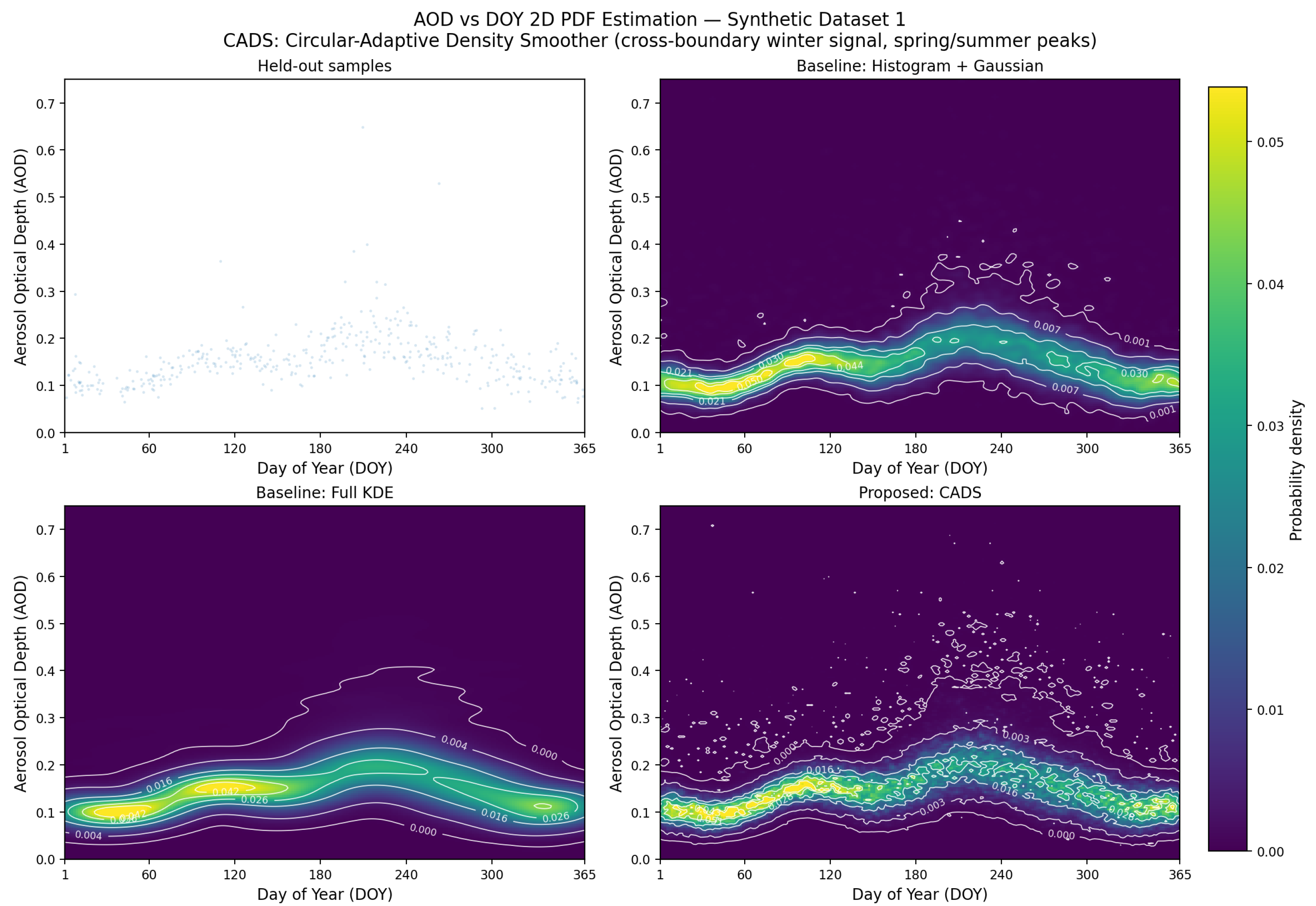
Figure 1 shows the density estimates for Synthetic Dataset 1. The histogram baseline produces a diffuse estimate that over-smooths the summer AOD peak and fails to resolve the cross-boundary winter signal. Standard bivariate KDE captures the main seasonal structure but exhibits an artificial discontinuity at the DOY $=1$ and DOY $=365$ boundary that is absent in the underlying data. CADS produces a smooth and continuous estimate that captures all three seasonal peaks and correctly connects the density at both ends of the annual cycle.

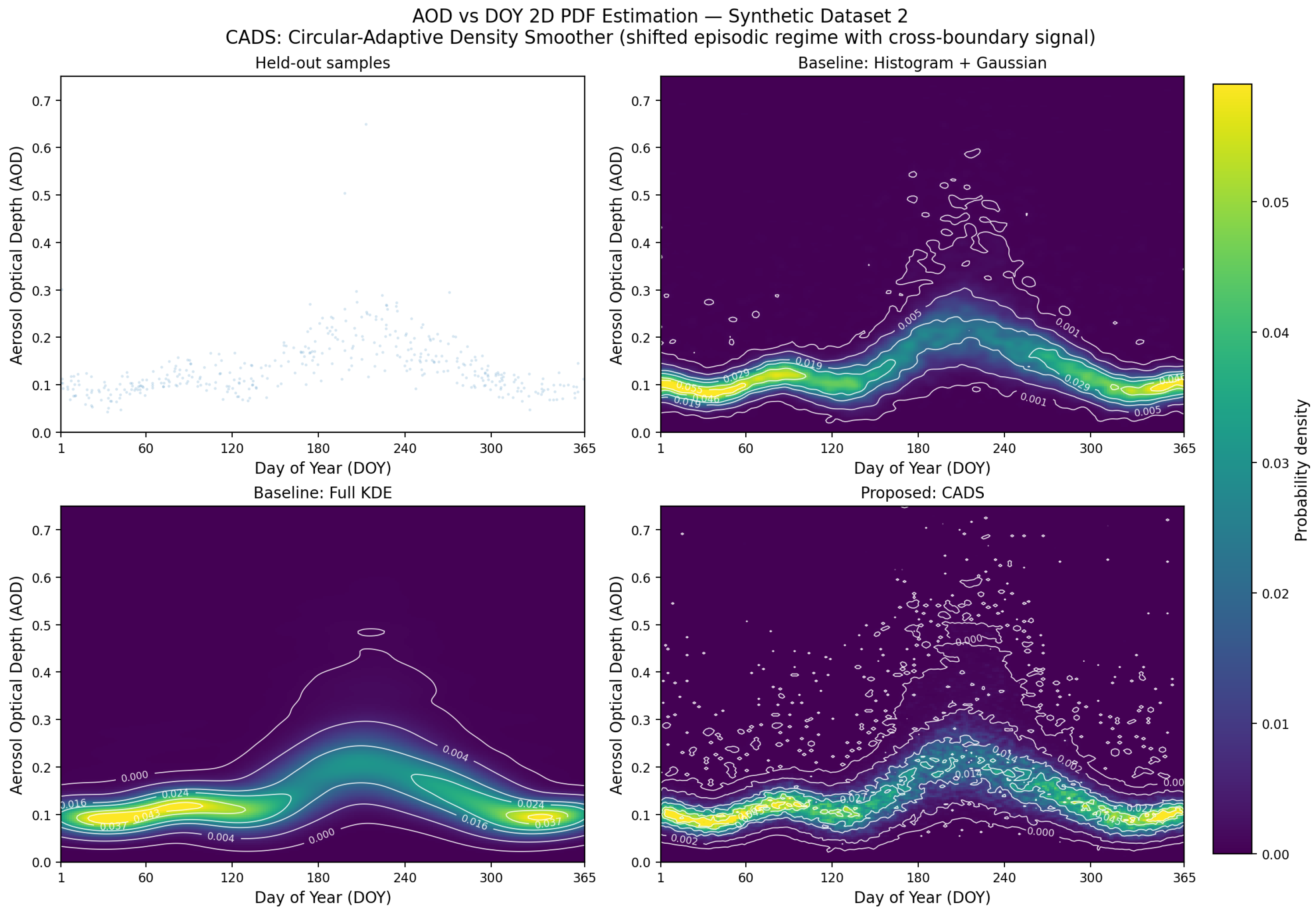
Figure 2 shows the results for Synthetic Dataset 2. Due to the sharper episodic structure in this synthetic dataset, the limitations of the histogram method are more apparent. The high-density episodic events across a range of AOD values are smoothed uniformly across the episodes. The standard bivariate KDE distribution displays boundary artefacts at the annual boundary between fall and spring. CADS produces a distribution that captures both the episodic and seasonal structure of the data and is continuous at the boundary between annual seasons.

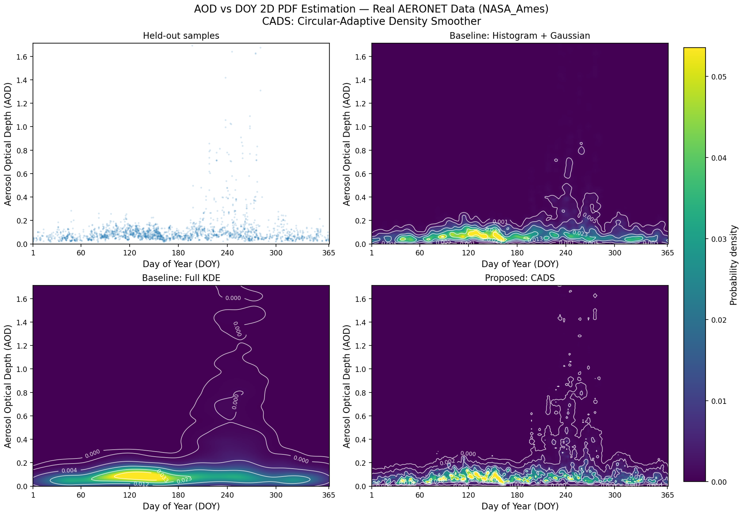
Figure 3 shows results for the AERONET NASA Ames dataset. The real observational data contain irregular temporal sampling, measurement noise, and sharp episodic events caused by wildfire smoke near DOY $=210$ to DOY $=280$. The histogram baseline lacks the resolution to capture the high-AOD smoke events and produces a noisy estimate in the upper AOD range. Standard bivariate KDE substantially over-smooths the summer smoke signal into an indistinct region and also shows a large boundary artefact at the annual transition. CADS provides a stable estimate that captures the low-AOD baseline across most of the year. It resolves the summer smoke signal as a distinct high-density region and maintains continuity at the annual boundary.

4.5. Ablation Study

Table 3. Ablation study of CADS components on Synthetic Dataset 1. C = Circular, A = Anisotropic, I = IPF. Higher logL and lower bdisc are better.

Config	Components	Mean logL	Mean Bdisc
C0	None	$-3.837$	$0.218$
C1	C only	$-3.837$	$0.111$
C2	A only	$-3.837$	$0.234$
C3	I only	$-3.834$	$0.144$
C4	C + A	$-3.837$	$0.108$
C5	C + I	$-3.834$	$0.078$
C6	A + I	$-3.834$	$0.155$
C7	C + A + I (Full CADS)	$-3.834$	$0.077$

and

Table 4. Ablation study of CADS components on Synthetic Dataset 2. C = Circular, A = Anisotropic, I = IPF. Higher logL and lower bdisc are better.

Config	Components	Mean logL	Mean Bdisc
C0	None	$-3.822$	$0.264$
C1	C only	$-3.822$	$0.130$
C2	A only	$-3.821$	$0.283$
C3	I only	$-3.816$	$0.175$
C4	C + A	$-3.821$	$0.117$
C5	C + I	$-3.816$	$0.086$
C6	A + I	$-3.816$	$0.188$
C7	C + A + I (Full CADS)	$-3.816$	$0.078$

report the ablation study results for Synthetic Datasets 1 and 2 respectively. Eight configurations are tested by independently enabling or disabling each of the three novel CADS components. The three components are circular boundary treatment (C), anisotropic adaptive smoothing (A), and IPF marginal correction (I).

The results are consistent across both datasets and support three conclusions.

The first conclusion concerns the IPF component. Comparing C0 to C3 shows a gain of $+0.003$ nats on Dataset 1 and $+0.006$ nats on Dataset 2 from IPF alone. No other single component produces a comparable gain in log-likelihood. IPF is therefore the primary driver of predictive improvement.

The second conclusion pertains to the treatment of the circular boundary component of the model. The circular component alone contributes to a 50% reduction in the bdisc metric for both datasets—from 0.218 to 0.111 for Dataset 1, and from 0.264 to 0.130 for Dataset 2. The circular component contributes minimally to the log-likelihood statistic due to few test points being located at the annual boundary; however, the geometric correction that the component provides is important for any application of the model requiring accurate representation of seasonal phenomena.

The third conclusion concerns the full CADS configuration. C7 achieves the lowest bdisc on both datasets and matches or exceeds the best log-likelihood of any partial configuration. Comparing C5, which uses circular treatment and IPF but not anisotropic smoothing, to C7 shows that adding the anisotropic component further reduces bdisc from $0.078$ to $0.077$ on Dataset 1 and from $0.086$ to $0.078$ on Dataset 2. This confirms that all three components contribute to the overall performance of the method.

5. Discussion

5.1. Performance on Real Versus Synthetic Data

The results show that CADS improves more substantially on real observational data than on synthetic datasets. The gain in held-out log-likelihood relative to the histogram baseline increases from $+0.014$ nats on Synthetic Dataset 1 to $+0.107$ nats on the real AERONET data. This is a 7.7-fold amplification. The gain relative to Standard bivariate KDE increases from $+0.028$ nats to $+0.314$ nats, which is an 11-fold amplification. This pattern is consistent and expected.

The synthetic datasets are generated from smooth parametric models with noise. The seasonal component of these synthetic datasets is regular. Hence, a histogram-based estimator can capture the seasonal component well, and the improvement brought about by CADS is not very significant. The real data from NASA Ames are very different from the synthetic data. The presence of sharp events in the data caused by wildfire smoke cannot be captured by smooth parametric models. These features introduce localised regions of high density in the AOD direction. Smoothing uniformly across the entire domain will spread these features over a large region. The density within the region where the events actually occur will be reduced, while the density in regions that contain no information about the events will increase. CADS compensates for this by automatically adapting to the regions that contain the events and those that do not, independently along each axis. Finally, IPF corrects differences between the marginal distributions of the estimated density and those directly observed in the data. Together, these methods produce a substantial improvement in the quality of the estimated density when applied to real data.

5.2. Role of Each Component

The ablation study allows the contribution of each component to be assessed independently. Three conclusions emerge consistently across both datasets.

The IPF marginal correction is the primary driver of improvements in the log-likelihood. Since smoothing tends to distort the marginal distributions, correcting this distortion improves the density estimate at test points. Furthermore, the IPF correction is performed at negligible computational cost, and convergence of the IPF iterations is guaranteed by the Sinkhorn–Knopp theorem [22]. The role of regularization to constrain model outputs to lie within the distribution of the observed data has been studied extensively in the context of statistical learning theory, where the compactness of the hypothesis class is intimately related to the existence of solutions to the learning problem and the convergence of those solutions to the true underlying distribution [34]. A similar principle is at the foundation of the IPF step within the CADS method, which enforces consistency of the univariate margins of the estimated distribution with the observed data.

The anisotropic smoothing component provides additional improvement, especially on Synthetic Dataset 2 and the real AERONET data. The difference between C3 and C7 on both the bdisc and log-likelihood metrics indicates that the anisotropic component provides improvements that are independent of the IPF component. This is consistent with the motivation for using anisotropic smoothing. Each of these quantities has physically distinct scales; it is therefore more accurate to calibrate the smoothing separately along each dimension than to use a single smoothing parameter for all dimensions.

The circular component has a different character from the other two components. Its contribution to the log-likelihood is negligible on both datasets, yet it reduces the boundary discontinuity metric by approximately 50%. The reason for this is that the log-likelihood on the held-out dataset is not sensitive to boundary discontinuities. The observations are drawn uniformly along the DOY axis, so few observations fall near the circular boundary. Thus, the boundary discontinuity metric D, defined in Equation (23), is the appropriate metric for evaluating this component. The reduction in D from 0.218 (without circular treatment) to 0.077 (in full CADS on Dataset 1) indicates a substantial improvement in the physical realism of the model. A density estimate that is discontinuous at the January–December boundary implies that the atmosphere behaves differently on day 365 than on day 1, which is physically impossible. Thus, any application of this model that depends on the atmosphere behaving continuously over time will be affected by this artefact.

5.3. Comparison with Standard Bivariate KDE

A notable result in Table 1 is that CADS outperforms Standard bivariate KDE on held-out log-likelihood despite being orders of magnitude faster. This may seem counterintuitive, since KDE is a nonparametric method with well-established theoretical properties. The explanation lies in bandwidth selection. Scott’s rule and Silverman’s rule are global selectors that choose a single bandwidth optimised for the overall data distribution. For data with highly non-uniform density, such as the AERONET dataset with its dense low-AOD baseline and sparse high-AOD smoke events, a global bandwidth necessarily over-smooths dense regions or under-smooths sparse ones. The locally adaptive scheme in CADS addresses this by adjusting smoothing strength at each grid cell based on local empirical support. The bandwidth sensitivity analysis in Section 4.2 confirmed that this conclusion is robust. Scott’s and Silverman’s rules produced identical results, so bandwidth selection is not the explanation for KDE’s weaker performance.

The computational advantage of CADS is also practically significant. On the AERONET dataset of $n=74,653$ observations, the standard bivariate KDE takes approximately 56 s per fold to estimate the KDE, while CADS takes only 0.019 s per fold. This represents a speedup of approximately 3000 times when using the full AERONET dataset of $n=74,653$ observations on a single CPU core. CADS computes the KDE on a fixed grid of $220\times 180$ pixels irrespective of the number of observations, n, while standard KDE must evaluate the bandwidth at each of the n observations, leading to computational costs of $O(N_X·N_Y)$ versus $O\left(n^2\right)$, respectively. Thus, for situations in which the density is to be estimated many times, such as in cross-validation or bootstrapping, the computational cost of CADS is considerably more favorable than that of the standard technique.

The computational complexity of CADS is $O(N_X·N_Y·log(N_X·N_Y))$ per density estimate. This computational complexity is independent of the number of observations, n, which is the case with the KDE algorithm. The additional cost of the IPF correction algorithm is $O(T·N_X·N_Y)$, which is negligible in the case of three categories of observations ($T=3$).

5.4. Limitations

Several limitations of the present study should be acknowledged.

The evaluation of the model with real data is available for only the NASA Ames site, which has a specific climate characterised by coastal fog and wildfire smoke. Other regions of the planet, with different types of aerosols, would likely lead to different results. Furthermore, many regions of the planet have limited availability of satellite data over time (due to, for example, the presence of clouds in that region), or have climates that are seasonal and monsoonal in character, which may also present challenges to the CADS methods that were not encountered in the relatively mild and coastal climate of California. Thus, evaluation of the method with these types of data is yet to be performed. Only through evaluation of the model on real data from various sites across the planet will the generalisability of the method become apparent.

To partially address this issue without collecting any additional data, the fact that the synthetic datasets were created to represent regimes of different seasonal characteristics can be mentioned. Dataset 1 was created to reflect seasonal characteristics that included weak winter regimes, while Dataset 2 was created to include regimes with stronger episodic characteristics and cross-boundary signals. CADS outperformed the other methods in both seasons. However, regions with sparse sampling, such as regions that are often covered in clouds in passive remote sensing, may present challenges to the application of the IPF step, indicating a need for future evaluation of these cases with the multi-site datasets.

The parameters of CADS, including the replication width W, the dense and sparse bandwidths, the density quantile threshold, and the number of IPF iterations, are set manually based on the characteristics of AOD-DOY data. The chosen values generalised well from synthetic to real data in this study. However, automating the parameter selection process would allow for CADS to be applied more broadly to other remote sensing data without requiring expert knowledge to tune the parameters.

The IPF correction relies on accurate estimation of the one-dimensional marginal distributions. Its performance may degrade with smaller sample sizes, with fewer seasonal observations, or with missing observations, such as those introduced by cloud contamination in passive remote sensing. In these situations, the empirical marginal distributions may not accurately represent the true marginal distributions, potentially introducing bias into the estimate.

Another limitation of the study relates to the temporal structure of the data. While the NASA Ames data has temporal autocorrelation, five-fold cross validation uses random sampling of the data. Furthermore, although CADS does not model year-to-year relationships within the satellite data, it is possible that five-fold cross validation does not accurately reflect the model’s performance on temporally-blocked test sets. Thus, future approaches to validating CADS could use blocked cross-validation techniques, such as leave-one-year-out cross validation, to evaluate the model’s robustness to temporally-blocked testing.

CADS operates on a fixed evaluation grid of size $220\times 180$. For applications outside of the original problem domain, it is likely that the parameters of the grid must be adjusted. Furthermore, the bandwidth parameters may also have to be re-tuned for such a case study.

6. Conclusions

This paper introduced CADS, the Circular-Adaptive Density Smoother, a computationally efficient method for two-dimensional probability density estimation of seasonal geophysical data. The method was motivated by three limitations of standard density estimators. The first is the failure to respect the periodic nature of the Day of Year axis. The second is the use of isotropic smoothing kernels that do not reflect the physically distinct scales of the two variables. The third is the marginal inconsistency introduced by any smoothing operation.

CADS addresses these three limitations through three independently motivated and individually ablatable components. The treatment of the circular boundary applies torus replication to the histogram prior to smoothing. This ensures that the density estimates at the January and December boundaries incorporate information from the opposite end of the year. The anisotropic locally adaptive smoothing scheme replaces the bandwidth with axis-specific bandwidths and a blending weight calculated from the data. It applies narrow smoothing in well-sampled regions and broad smoothing in poorly sampled regions, independently along the DOY and AOD dimensions. Iterative Proportional Fitting then enforces consistency between the smoothed estimates and the empirical univariate distributions. This removes bias introduced by the smoothing process at negligible computational cost.

Experiments on two synthetic datasets and one real AERONET observational dataset show that CADS achieves the highest mean log-likelihood across all datasets. All improvements are statistically significant. The improvements are particularly pronounced on the real data. The gain achieved by CADS over histogram methods is 7.7 times larger on the real data than in the synthetic datasets, and the gain over Standard bivariate KDE is 11 times larger. Furthermore, CADS is approximately 1500 to 3000 times faster than Standard bivariate KDE. Finally, an ablation study of CADS indicates that each component makes an independent contribution to its performance: the IPF component is responsible for most of the increase in log-likelihood, the circular treatment explains the reduction in boundary discontinuity, and anisotropic smoothing provides additional gains in both metrics.

There are three directions for future work. One direction involves expanding the evaluation to multiple AERONET sites that represent different climatic regimes. Such an approach would enable a thorough assessment of the generalisability of the method. Another direction for future work involves automating the selection of the smoothing bandwidth parameters. An automated approach would reduce the need for manual tuning of the method, which would increase its applicability to other domains. Finally, it may be possible to extend the CADS approach to higher dimensions. For instance, another dimension that could be included is the spatial coordinate of the measurement location, such as latitude or longitude. This dimension could be used to model seasonal and spatial variations in the measurements.