Article

Experience Extractor for Adaptive Tradeoff Between Exploration and Exploitation in Reinforcement Learning

by
Zhi Yi
,
Zhongmin Wu
,
Yongming Xie
,
Ming Chen
and
Yinglong Dai
*
Hunan Provincial Key Laboratory of Intelligent Computing and Language Information Processing, College of Information Science and Engineering, Hunan Normal University, Changsha 410081, China
*
Author to whom correspondence should be addressed.
Mathematics 2026, 14(10), 1624; https://doi.org/10.3390/math14101624
Submission received: 8 April 2026 / Revised: 4 May 2026 / Accepted: 7 May 2026 / Published: 11 May 2026
(This article belongs to the Special Issue Applications of Intelligent Game and Reinforcement Learning)

Abstract

In Reinforcement Learning (RL), the agent cannot distinguish between exploratory and exploitative experience. Not all sequential experiences contribute equally to the agent’s optimization, and the same experience holds different importance at different learning stages. We propose the Extractor for Adaptive Tradeoff Between Exploration and Exploitation (EATBEE), a task-oriented tool that tightly couples with the agent’s current knowledge and enables adaptive knowledge acquisition. We compare the originally sampled data with the task-driven data distribution to clearly illustrate their deviation. Then, we show how EATBEE identifies and extracts beneficial data for the agent. The monotonic improvement policy is theoretically validated under the assumption that the experience trajectory keeps a high degree of trajectory similarity after extraction. EATBEE serves as an independent module that can be seamlessly integrated with most existing RL algorithms. We substantiate the efficacy and practical applicability of the EATBEE method through experiments conducted in both discrete and continuous environments.

1. Introduction

The analysis of sequential data plays a crucial role in Reinforcement Learning (RL), particularly in addressing the tradeoff between the exploration and exploitation in policies [1,2]. Specifically, if the RL model explores excessively, the policy may fail to converge; conversely, insufficient exploration can cause the policy to get trapped in local optima [3,4]. Consequently, the performance of an RL model is significantly influenced by the quality of the sampled data [5,6]. Currently, existing approaches primarily rely on expert data to improve the quality of RL samples, which significantly improves the performance of policy models [7,8,9]. However, such methods require prior knowledge and meticulous manual intervention. The ultimate objective of artificial intelligence (AI) has not only been to imitate human behavior, but also to enable autonomous exploration in unknown domains and to surpass existing human expertise [10,11].
The most representative class of exploration algorithms is based on curiosity-driven exploration. In this paradigm, exploration signals are intrinsically generated from the agent’s state prediction error, thereby decoupling it from the extrinsic reward provided by the environment. Representative methods include the Intrinsic Curiosity Module (ICM) [12], Random Network Distillation (RND) [13], and DreamGym [14]. This category of algorithms has also been extensively leveraged in vision-language models (VLMs) to improve policy performance [15]. Other major categories include methods based on state visitation counts [16,17,18], and state entropy maximization [19,20,21]. We find that exploration algorithms that effectively balance exploration and exploitation are better at boosting policy performance. To this end, we propose a key insight: policy sampling data should maintain an optimal tradeoff between exploration and exploitation. Rather than encouraging broad exploration, our approach extracts experiences that best align with the agent’s learning stage.
Exploration and exploitation in RL have long been extensively studied [22,23,24,25]. In sparse reward environments, which are common in real-world scenarios, a fundamental challenge lies in the tradeoff between exploration and exploitation. Specifically, agents often fail to perceive the direction of task progression, leading to excessive exploration that marginalizes the importance of exploitation data for policy optimization. We evaluate our approach in sparse-reward regimes, where infrequent feedback exacerbates the risks of stochastic exploration and underscores the necessity of an adaptive tradeoff between exploration and exploitation. (Sparse-reward regimes represent the prevalent real-world paradigm of RL, because reward engineering is notoriously intricate and rarely yields fine-grained, reliable shaping. This setting simultaneously offers a transparent testbed: the near-absence of external feedback strips away confounding supervisory signals and allows us to isolate, simplify, and theoretically ground the contribution of our method.) Notably, the term “extensive exploration” in our context refers to local-level exploration, which aligns with many existing studies [26,27,28]. While most prior work emphasizes balancing exploration and exploitation by encouraging agents to explore broader regions of the state space, our approach differs fundamentally. We focus not on expanding the scope of exploration, but rather on identifying and leveraging exploitation data from the sequential experiences [29]. By adaptively capturing the most beneficial data distribution from the original dataset, we aim to improve the policy more effectively while preserving its exploratory capabilities. Therefore, we propose the Extractor for Adaptive Tradeoff Between Exploration and Exploitation (EATBEE), a tool that facilitates a more effective and efficient policy optimization process.
Inspired by dense RL [30], we aim to dynamically adjust the proportion of exploration and exploitation data in sampled trajectories, based on the current policy and the agent’s task-specific epistemic. Specifically, we propose a data truncation mechanism that adaptively balances exploration and exploitation. We posit that effective exploration enhances the agent’s understanding of the underlying task structure, while proper exploitation allows it to perform the task more efficiently. Therefore, when the agent lacks sufficient understanding, we encourage increased exploration. Conversely, when exploration becomes excessive relative to the task knowledge acquired, we shift the focus toward exploitation. Our work differs from dense RL, where algorithms like Deep Q-Network (DQN) [31] are evaluated without explicitly considering the sequential dependencies in trajectory experience. In contrast, we introduce an adjacency network [32] that embeds truncated segments into a shared embedding space, preserving their contextual similarity—a property we refer to as reachability. This ensures that the temporal structure and semantic coherence among sequential data are minimally disrupted. Furthermore, building upon the policy gradient theorem, we theoretically demonstrate that our method guarantees monotonic policy improvement in sparse reward environments. Finally, we evaluate our approach across multiple benchmark tasks and demonstrate that EATBEE outperforms state-of-the-art baselines, validating both its theoretical soundness and practical effectiveness.
The main contributions of this paper are as follows:
1.
We propose an experience extractor, EATBEE, which can be integrated with most RL algorithms.
2.
We establish a theoretical foundation guaranteeing that EATBEE achieves monotonic improvement in sparse reward environments.
3.
We provide an intuitive visualization of the EATBEE mechanism to elucidate its underlying dynamics.
4.
We conduct evaluation experiments in both low- and high-dimensional state and action environments with sparse or dense rewards. The results show that EATBEE outperforms the baseline and exhibits greater robustness and stability.
The novelty of EATBEE lies in (1) extracting task–beneficial experiences instead of expanding exploration; (2) adaptive trajectory pruning with reachability preservation; (3) stage-aware sample selection via double value functions; (4) a plug–and–play, algorithm-independent module.
The remainder of this paper is organized as follows. After motivating our approach through a discussion of the exploration–exploitation tradeoff in Section 1, we review the relevant literature on experience replay and exploration strategies in Section 2. Section 3 then establishes the formal mathematical preliminaries necessary for the subsequent derivation. The core methodology is detailed across three subsequent sections: Section 4 elaborates on the operational principles of EATBEE, including its correlation metrics and a proof of monotonic performance improvement; Section 5 discusses data optimization under reachability constraints; and Section 6 describes how EATBEE adaptively refines sampled data to enhance policy training quality. These theoretical contributions are followed by Section 7, which provides comprehensive experimental validation, ranging from data distribution analysis to policy performance benchmarks and transferability tests. Finally, Section 8 concludes the paper with a summary of our findings.

2. Related Work

2.1. Exploration and Exploitation

The tradeoff between exploration and exploitation remains one of the foundational challenges in RL [33]. Existing RL policies often suffer from a lack of sufficient exploration, frequently leading them to converge to suboptimal policies [34]. The direct approach is to maximize policy entropy [35,36]. Specifically, the main goal of RL exploration is to visit unknown states, not merely to cover the entire state space. This realization has spurred the development of various auxiliary components designed to enhance a policy’s visitation of these unknown states. For instance, ICM constructs an intrinsic reward based on the prediction error of the next state to encourage the agent to explore novel state regions [37]. In addition to curiosity-driven exploration, methods like state visitation counts [38,39] and state entropy maximization [40] all primarily aim to facilitate the agent’s access to unknown states. This naturally raises a question: are these unknown states necessarily relevant information gains for the current task? To address this, we propose EATBEE, a novel data-driven method for the adaptive tradeoff between exploration and exploitation in a specific-task context. Its primary advantage lies in its ability to capture the underlying task distribution trend of the task and dynamically adjust the tradeoff strategy.

2.2. Experience Replay

The tradeoff between exploration and exploitation aims to obtain high-quality data for effective policy learning. Experience Replay (ER) [31] improves sample efficiency by uniformly sampling transitions from an experience buffer. However, it does not meet the requirements of the evolving policy. Prioritized Experience Replay (PER) [41] increases the sampling probability of transitions with higher temporal-difference error. This mechanism guides the agent to revisit informative experiences and explore less-visited regions of the state space. However, excessive exploration is inefficient in unknown regions, as many areas of the state space may be irrelevant to the specific task. Modern AI systems are designed to rapidly obtain task-relevant knowledge and outperform humans in task completion efficiency. An experience replay method based on frequency and similarity (FSER) [42] was proposed, which prioritizes transitions that are rarely sampled or highly relevant to the current policy, to alleviate imbalanced sampling. FSER and our approach, though conceptually related, pursue distinct functional goals. FSER focuses primarily on alleviating catastrophic forgetting; by contrast, we endeavor to balance the inherent tradeoff between exploration and exploitation through optimized experience selection, improving data quality.
Our research is primarily inspired by dense RL [30], which performs backpropagation within specific regions of the state space. However, it remains agnostic to the agent’s knowledge requirements, thereby lacking task-driven adaptability. Furthermore, we posit that not all states within a trajectory contribute equally to backpropagation or policy updates. By combining FSER and dense RL, our research aims to achieve an adaptive tradeoff between exploration and exploitation, enabling an agent to capture task-relevant knowledge from trajectories. EATBEE fundamentally differs from existing exploration–exploitation approaches in three key ways: (1) Instead of encouraging broader state-space exploration (e.g., curiosity, count, entropy maximization), EATBEE extracts task-aligned experiences from sampled trajectories to adaptively balance exploration and exploitation; (2) Unlike PER and FSER, which focus on sampling weights, EATBEE performs trajectory-level structured pruning while preserving Markovian reachability; (3) Different from dense RL, EATBEE uses policy-aware adaptive thresholds (double value functions, knowledge coefficient and latent state space) to match the agent’s learning stage, rather than fixed backpropagation regions.

3. Preliminaries

We consider the RL problem within the framework of Markov Decision Processes (MDPs). MDPs are usually defined by the tuple < S , A , P , r , γ > , where S is a state space, A is an action space, P : S × A S is a state transition function, r : S × A × S R is an immediate reward function, and  γ [ 0 , 1 ) is the discount factor. The objective of RL is to maximize the expected cumulative return:
J ( θ ) = E π θ [ G ( τ ) | s 0 ] ,
given the state s 0 under the policy π θ ( a | s ) parameterized by θ , where G ( τ ) = t = 0 γ t r t and τ is the trajectory of the agent’s sampling. The agent samples a sequential experience trajectory
τ = { ( s 0 , a 0 , r 0 ) , ( s 1 , a 1 , r 1 ) , , ( s T , a T , r T ) } | T 0 ,
where the transition ( s i , a i , r i ) depends on the previous experience
{ ( s 0 , a 0 , r 0 ) , , ( s ( i 1 ) , a ( i 1 ) , r ( i 1 ) ) } | i 1 .
According to the policy gradient theorem, the gradient of the objective J ( θ ) is given by
θ J ( θ ) = E π θ [ t = 0 θ l o g π θ ( a t | s t ) G ( τ ) ] .
Then, θ is updated as θ θ + α θ J ( θ ) , where α is the learning rate. To reduce the variance in the policy gradient, we introduce the state-value function V ( s ) = E π θ [ G ( τ ) | s ] and the action-value function Q ( s , a ) = E π θ [ G ( τ ) | s , a ] , parameterized by ϕ V and ϕ Q , respectively.

4. The Extractor of Sequentially Sampled Data

4.1. Sequential Experience Data Extraction

Let π denote a stochastic policy that induces a trajectory τ over a finite time horizon T, defined by
τ = { ( s 0 , a 0 , r 0 ) , ( s 1 , a 1 , r 1 ) , , ( s T , a T , r T ) } ( S × A × R ) T + 1 .
We define a latent state space X , and assume the existence of a forward mapping function W : S X that maps observations to the latent space, along with an inverse mapping M : X S such that s = M ( W ( s ) ) for any observation s.
The latent state space X we construct exhibits structural properties analogous to those of the adjacency matrix space [32]. We introduce a hyperparameter c to indicate the agent’s capability to reach a specific state within c steps. A detailed description is provided in Section 5. By mapping a complete trajectory τ into the latent state space X , i.e.,  τ X = W ( τ ) , we construct an observation correlation matrix C R ( T + 1 ) × ( T + 1 ) that encodes pairwise relationships among latent states along the trajectory. We also define a correlation threshold κ (in our work, we set κ = 0.99 by default). One effective application is to compute the correlation between any two arbitrary latent variables within the latent state space X , aiming to identify the optimal data distribution along a trajectory. Its core advantage lies in improving data quality while preserving both the Markov property and the reachability of states. For the data x X j following the latent state x X i where j > i , if  c o r r ( x X i , x X j ) > κ = 0.99 , then the segment { s i , , s j 1 } can be eliminated, where c o r r is the correlation calculation function. In our work, c o r r is set as the Pearson correlation coefficient function, given by
ρ X , Y = c o v ( X , Y ) σ X σ Y = E [ ( X μ X ) ( Y μ Y ) ] E [ ( X μ X ) 2 ] E [ ( Y μ Y ) 2 ] ,
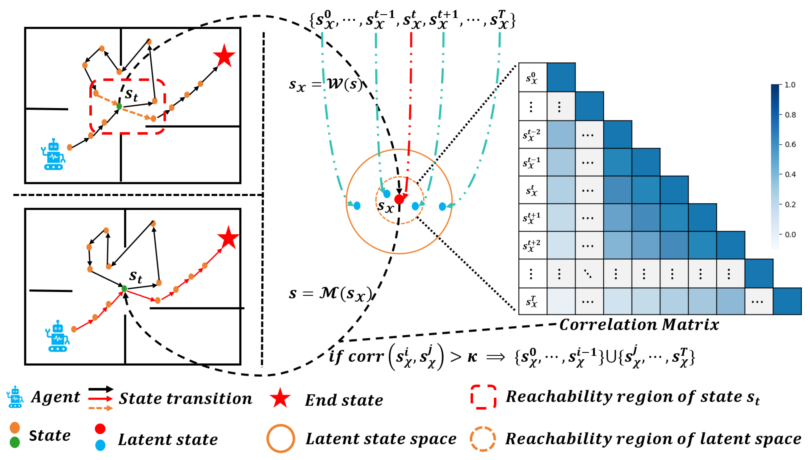
where c o v ( X , Y ) is the covariance, and μ and σ denote the mean and standard deviation, respectively. Correlation is adopted as a pruning criterion for its efficiency in measuring state redundancy and preserving trajectory structural consistency. We emphasize that correlation is a choice for discrete environments, not a mandatory core of EATBEE. In continuous spaces, we switch to value-based significance filtering. The extraction is valid only when both similarity and reachability are satisfied, ensuring the Markov property and task reward are preserved. Correlation can be replaced by cosine similarity or Euclidean distance without breaking the framework. The conceptual framework of EATBEE is illustrated in Figure 1.
The EATBEE extracts the outcome from τ :
τ E A = ( s 0 E A , a 0 E A , r 0 E A ) , ( s 1 E A , a 1 E A , r 1 E A ) , , ( s n E A , a n E A , r n E A ) | n T ,
where τ E A represents the new trajectory obtained by processing τ . Although ( s i , a i , r i ) = ( s i E A , a i E A , r i E A ) may not hold in general, r T = r n E A must be satisfied; that is, the reward at the final step must be equal because the extractor must ensure that the same final state is reached. Consequently, the extractor only performs improvements on the intermediate steps of a trajectory. We define the cumulative return along trajectory τ at time t as G t = i = t T γ i t r i , and the cumulative return of the EATBEE-augmented trajectory τ E A is given by G t E A ( τ ) = i = t n γ i t r i E A , where t < n T . We observed that, in a continuous state space, the correlation matrix is computationally challenging to estimate, which prevents the experience extractor from achieving an adaptive tradeoff between exploration and exploitation. Therefore, we explored an alternative method for expansion. Details on how to obtain τ E A in a continuous observation space are provided in Section 6.

4.2. EATBEE Conditional Monotonic Improvement Theorem

To quantify the effectiveness of EATBEE in improving data quality, we introduce a metric called the return difference ratio.
Definition 1 (Return Difference Ratio).
Given a trajectory τ under policy π, let G π ( τ ) and G π E A ( τ ) denote the returns under the original and EATBEE-augmented trajectories, respectively. The return difference ratio is defined as
δ = G π ( τ ) G π E A ( τ ) .
Thus, δ can be expressed as follows:
δ = G t ( τ ) G t E A ( τ ) = i = t T γ i t r i | t < n T i = t n γ i t r i E A | t < n T .
The metric reveals the following insights: (1) during the initial learning phase of the policy, δ 0 , indicating EATBEE achieves significant performance improvement; and (2) when the agent successfully completes the task, as indicated by δ 1 , the improvement effect gradually diminishes.
Suppose the agent receives a fixed reward e at each step, and the reward for successfully completing the task is denoted by r T . After applying EATBEE, the number of steps along a trajectory τ with a finite horizon T is reduced to T k , where 0 k < T . Consequently, the returns G t ( τ ) and G t E A ( τ ) can be expressed, respectively, as follows:
G t ( τ ) = i = t T γ i t r i = e + γ e + γ 2 e + + γ T t r T ,
G t E A ( τ ) = i = t T k γ i t r i E A = e + γ e + γ 2 e + + γ T k t r T k E A .
Clearly, when k = 0 , we have G t ( τ ) = G t E A ( τ ) . If the environment provides sparse rewards (i.e., e = 0 ), we obtain
δ = G t ( τ ) G t E A ( τ ) = γ T t r T γ T k t r T k E A = γ k ( 0 δ 1 ) ,
The intuition of δ is to quantify the scale-up of the return, i.e.,  G t E A = G t γ k . However, δ is not a fixed value—it is dynamically determined by EATBEE. We observe that the improvement in EATBEE grows exponentially.
Our method is based on a key insight: the policy π = { π 0 , , π T } can be viewed as a sequence of sub-policies, where the future sub-trajectory { s t , , s T } is generated by a sub-policy π t . Since π t is a stochastic policy, the same sub-policy may lead to different state transitions. Consequently, in a trajectory τ = { s 0 , , s T } , the new trajectory τ E A = { s 0 , , s i 1 , s j , , s T } extracted by EATBEE may result from the sub-policy π i 1 . Thus, we introduce a lemma on the policy set for a trajectory τ .
Lemma 1 (Policy Distribution Mapping).
Given a trajectory τ = { s 0 , s 1 , , s T } , the sub-trajectory S i = { s i , s i + 1 , s T } is generated by the sub-policy π i of the policy π = { π 0 , π 1 , , π T } .
The goal of EATBEE is to obtain the optimal policy,
π * = { π 0 * , π 1 * , π 2 * , , π T k * | 0 k < T } ,
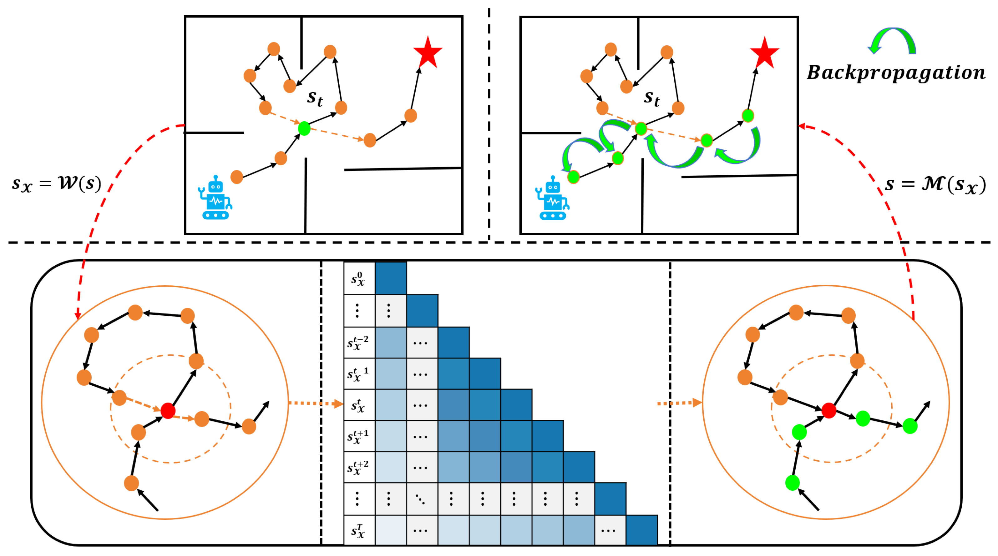
along a trajectory τ . Corresponding to π * , the optimal trajectory is defined as τ * = { s 0 , s 1 , , s T k | 0 k < T } under the same condition. Therefore, the optimal policy π * can be derived from the optimal trajectory τ * , as illustrated in Figure 2.
The new objective function after experience extraction can be formally defined as follows, given the state s:
J E A ( θ ) = E π θ [ G E A ( τ ) | s ]
A theorem [43,44] can be used to evaluate the performance improvement of the policy, and is formally stated as follows.
Theorem 1 
(Performance Difference Theorem [43,44]). For any two policies π and π, the performance difference
J ( π , π ) J ( π ) J ( π )
can be measured using the advantage function
J ( π , π ) = E τ P π ( τ ) [ t = 0 T γ t A π ( s t , a t ) ] = E s P π ( · ) , a π ( · | s ) [ A π ( s , a ) ]
Based on Theorem 1 and Equation (5), we derived the EATBEE Monotonic Improvement Theorem as follows.
Theorem 2 (EATBEE Conditional Monotonic Improvement Theorem).
In a sparse reward environment, where routine actions yield a zero immediate reward ( r = 0 ) and the terminal action (task success or failure) yields a non-zero reward ( r T 0 ), the monotonic improvement of EATBEE can be formally stated as follows:
J ( π , π ) = J E A ( θ ) J ( θ ) = ( 1 δ ) J E A ( θ ) 0
where δ = γ k , and k is a positive integer. The proof is provided in Appendix A.
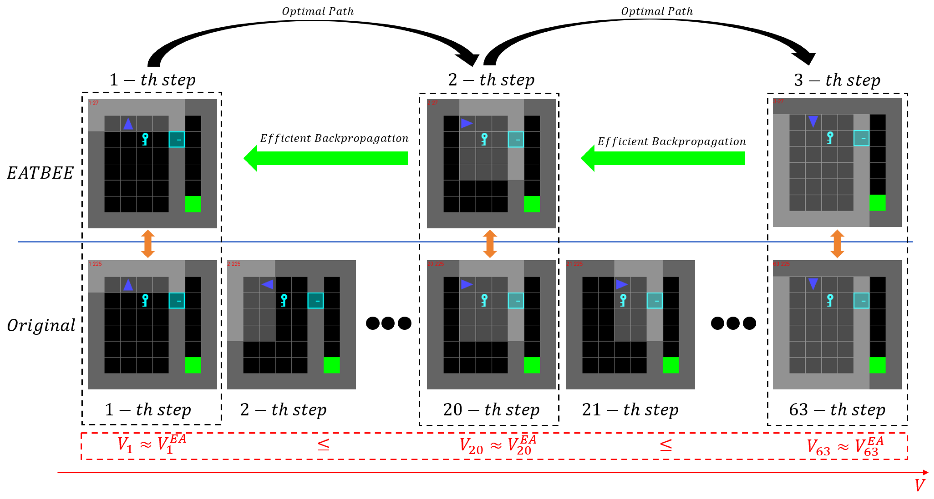
If J ( π , π ) > 0 , this indicates that the updated policy π outperforms the original policy π . Therefore, maximizing J ( π , π ) leads to an improved policy π that is guaranteed to perform at least as well as, and potentially better than, the current policy π . In this context, the term J E A ( θ ) is equivalent to J ( π ) , representing the performance of the updated policy. In a sparse reward environment, regardless of whether the task completion explicitly satisfies J E A J ( θ ) , it still holds that J E A ( θ ) J ( θ ) = γ k . Meanwhile, the backpropagation mechanism of EATBEE is illustrated in Figure 3. We do not claim universal monotonic improvement for all scenarios. Instead, EATBEE provides conditionally monotonic policy improvement under sparse rewards, high trajectory similarity, and valid reachability constraints.
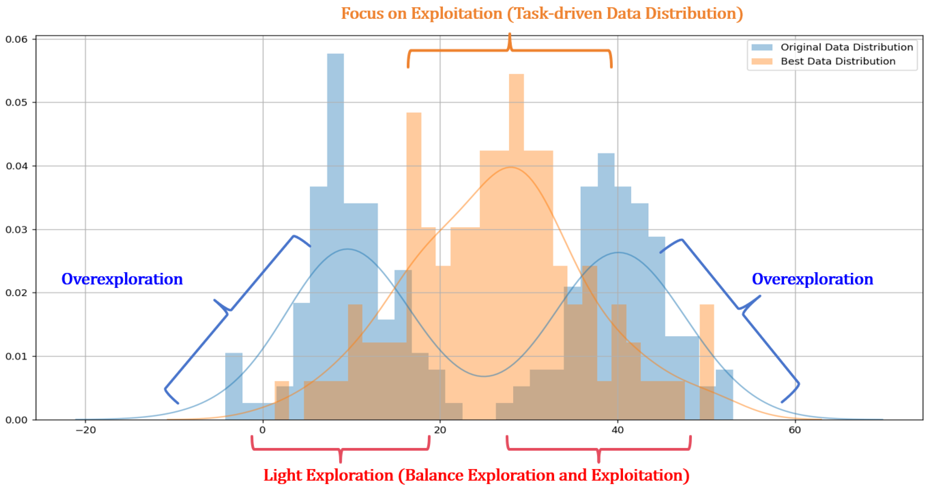
Let the distribution of the sampled data be denoted by f ( x ) , the optimal data distribution by g ( x ) , and the data deviation distribution by h ( x ) . These distributions are related by g ( x ) = f ( x ) h ( x ) . The unknown data distribution ratio can be expressed as ϕ = f ( x ) g ( x ) = 1 1 ϵ , where ϵ = h ( x ) f ( x ) represents the relative deviation from the sampled distribution. The characteristics of these data distributions are illustrated in Figure 4. EATBEE effectively mitigates the issue of excessive exploration and extracts a task-driven data distribution from the sampled data, thereby addressing the fundamental challenge of balancing exploration and exploitation.
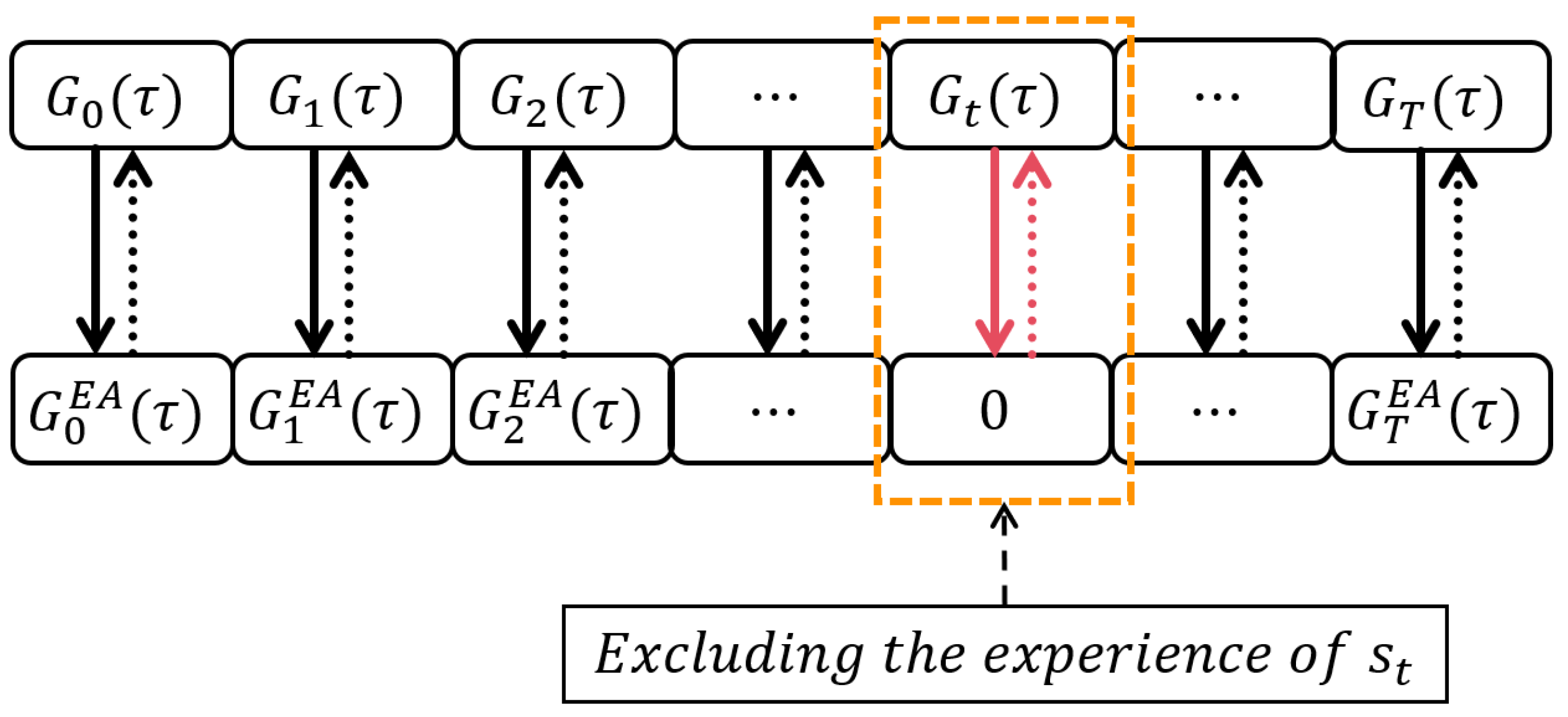
To preserve the generality of EATBEE, we implement the adaptive tradeoff with respect to the return G ( τ ) , rather than the immediate reward r. If a state s t is excluded by EATBEE, the corresponding return at that timestep is set to G t E A ( τ ) = 0 , as illustrated in Figure 5. Furthermore, EATBEE improves policy learning and stabilizes the value functions Q ( s , a ) and V ( s ) by reducing the learning burden on the neural network.

5. Trajectory Similarity

The experience extractor requires maintaining a high degree of similarity between trajectories τ and τ E A . We introduce a sequential data similarity metric, termed sequential data similarity.
Definition 2 (Sequential Data Similarity).
Consider sequential data X = { x 1 , x 2 , , x n } , where x i R m ( m > 0 ) . For any two sequences X 1 and X 2 , given a threshold ξ [ 0 , 1 ] , and  N Z + > 0 such that f ( X 1 , X 2 ) > ξ iff n > N . Furthermore, lim n f ( X 1 , X 2 ) 1 .
Evaluating the similarity between two sequences is significant, as it effectively preserves the inherent information. However, computing similarity over entire sequential data may incur substantial computational costs. To mitigate this, we observe that if a sequence X exhibits high similarity with and without a fragment X m = { x i + 1 , , x j } , where X m X , 0 i < j , this indicates x i x j . The sequence extracted by EATBEE is denoted as X E A . Therefore, the similarity calculation f ( X , X E A ) between X and X E A can be approximated by f ( x i , x j ) , i.e.,  f ( X , X E A ) f ( x i , x j ) . Accordingly, we introduce a simplified similarity evaluation method.
Proposition 1 (Simplified Sequential Data Similarity).
Under Definition 2, the similarity of the sequence X can be denoted as f ( X , X E A ) f ( x i , x j ) with and without a segment X m = { x i , , x j } | 1 i < j where X m X , i.e.,  x i x j .
Under Proposition 1, given a trajectory τ = { s 0 , s 1 , , s T } , if  s i s j , then the similarity f ( τ , τ E A ) can be approximated by f ( s i , s j ) , i.e.,  f ( τ , τ E A ) = f ( s i , s j ) . However, τ E A suffers from a limitation: the sequential reachability of τ E A may not be satisfied. This implies that, while the similarity condition f ( τ , τ E A ) f ( s i , s j ) > ξ holds, the extracted trajectory τ E A does not necessarily satisfy the Markov property in the original sequential data. To address this issue, we introduce the sequential data reachability metric.
Definition 3 (Sequential Data Reachability).
For any sequential data X = { x 1 , x 2 , , x n } in the sequential data space Γ, adjacent elements must satisfy reachability, i.e.,  x i 1 x i . Given a threshold η, adjacent elements must satisfy h ( x i 1 , x i ) η , where h ( · , · ) is a distance function.
According to Definition 3, given sequential data X = { x 0 , x 1 , , x n } , for any elements x i and x j , the transition x i x j + 1 is considered reachable iff h ( x i , x j + 1 ) h ( x j , x j + 1 ) η . Under Proposition 1 and Definition 3, the sequential data similarity can be formalized as follows:
f ( X , X ) f ( x i , x j ) s . t . i < j h ( x j , x j + 1 ) h ( x i , x j + 1 ) ,
where the measure h ( x i , x j ) is typically the Euclidean distance:
h ( x i , x j ) = | | x i x j | | 2
For a trajectory τ = { s 0 , s 1 , , s T | T > 0 } , the similarity can be formalized as follows within the reachability:
f ( τ , τ E A ) f ( s i , s j ) > ξ s . t . 1 i < j h ( s j , s j + 1 ) h ( s i , s j + 1 )
Under a deterministic constraint, directly computing the similarity along a trajectory τ is computationally expensive and often infeasible. To address this, we construct a latent space X to compute similarity for τ , inspired by the adjacency matrix [32]. We define a mapping function W : S X and a reverse mapping function M : X S , parameterized by θ W and θ M , respectively. To satisfy reachability within c steps in the latent space X , the loss function for the parameter θ W is defined as
L o s s X = y · h ( · , · ) l 1 + ( 1 y ) · l 2 h ( · , · )
where l 1 > 0 and l 2 > l 1 are constants defining the margin, and y { 0 , 1 } is a binary label indicating reachability (1 if reachable, 0 otherwise). We embed the reachability constraint directly into the latent state space X .

6. Adaptive Tradeoff

We introduced the experience extractor, which improves the data quality and policy learning by leveraging correlations under similarity and reachability conditions. However, directly using correlation presents two problems: (1) we need to manually remove the fragment X m = { x i + 1 , , x j } , then concatenate { x 0 , , x i } with { x j + 1 , , x T } when x i x j , and (2) correlation cannot capture the adaptive tradeoff. This approach is accurate and theoretically sound, yet it is computationally expensive. And the experience extractor exhibits suboptimal performance in continuous state tasks and lacks adaptability. We define ‘adaptability’ specifically as the strategic alignment of data requirements with the current policy’s learning stage. Specifically, the agent should prioritize extensive explorative data during the initial phases rather than focusing solely on exploitative data. As the policy gains task-specific knowledge, the data distribution should shift to maintain a high degree of exploitation while retaining a calibrated level of exploration. We developed an adaptive tradeoff approach to address the aforementioned issues. We utilize Proximal Policy Optimization (PPO) [45] as our baseline RL algorithm, with the objective function defined as follows:
L ( ϕ V ) = E V ϕ V π ( s t ) G t ( τ ) 2
L ( θ ) = E m i n π θ ( · | s ) π o l d ( a | s ) A π o l d ( s , a ) , c l i p π θ ( · | s ) π o l d ( a | s ) , 1 2 ϵ , 1 + 2 ϵ A π o l d ( s , a )
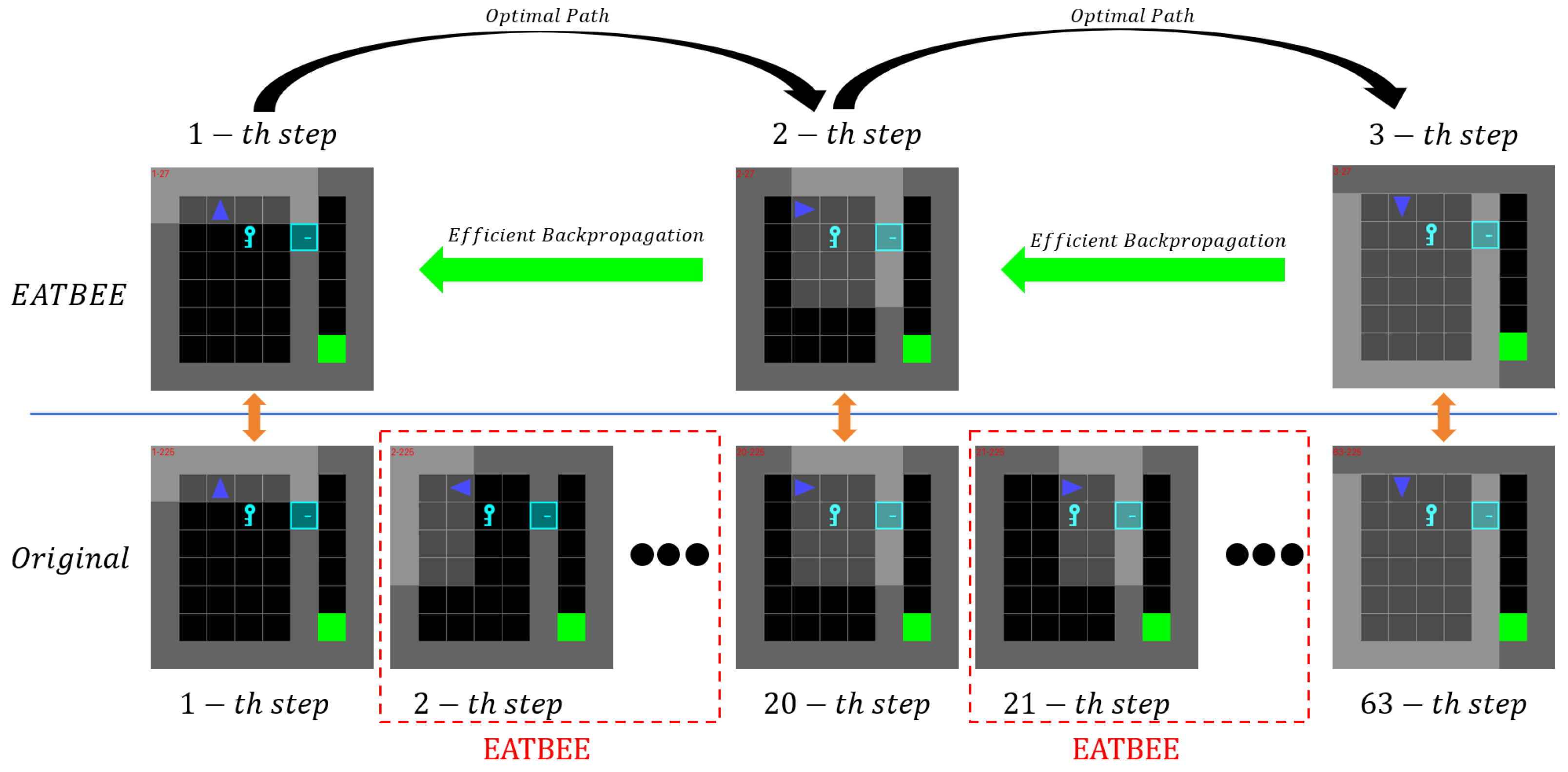
where π o l d represents the behavior policy from the previous iteration. The pseudocode for the EATBEE algorithm is presented in Algorithm 1. The actual performance is shown in Figure 6. In this scenario, there exists an expert who efficiently filters the data while preserving the MDP property, as expressed in Equations (4) and (7).
We posit that the adaptive tradeoff serves as the mediator between the policy and the task. We construct a parameterized function for the experience extractor. This function enables automated data pruning, thereby achieving an adaptive tradeoff between exploration and exploitation. Specifically, we design a neural network architecture, the state selection mechanism, to dynamically identify and select high-quality and informative data segments along the current policy π within the latent state space X .
Algorithm 1 EATBEE
  1:
Initialize: agent, replay buffer D .
  2:
while not converged do
  3:
    Agent collects trajectories τ D .
  4:
    if episode terminates then
  5:
        Sample all trajectories τ D .
  6:
        Update the adjacency latent space using Equation (11).
  7:
         τ E A τ using Equation (1).
  8:
        Update agent with τ E A .
  9:
    end if
10:
end while
It is crucial to note that EATBEE is designed to be continuously adaptive to the evolving current policy π . This implies that the state selection mechanism must dynamically align with π at all times. The most straightforward form of EATBEE is the value function. To formalize the update process, we introduce the concepts of the significant point and significant baseline to refine the state selection mechanism, as detailed in Definition 4.
Definition 4 (Significance Evaluation).
Given a trajectory
X = { x 1 , x 2 , , x T } ,
an element x X is called a significant point if f ( x ) > 0 , where the function f ( x ) : X R is referred as the significant baseline.
Considering a trajectory
τ = { ( s 0 , a 0 , r 0 ) , ( s 1 , a 1 , r 1 ) , , ( s T , a T , r T ) }
collected by the current policy π, if a state–action pair ( s , a ) satisfies
f ( s , a ) = Q t r u e ( s , a ) V π ( s ) > 0 ,
then it is considered a significant point, where f ( · ) serves as the significant baseline for π, Q t r u e ( s , a ) is the true state–action value, and  V π ( s ) is the predictive state value.
To mitigate the overestimation bias in value functions, which could lead to a severely distorted knowledge distribution, we employ a double state-value mechanism. This approach is conceptually analogous to Double Q-learning. We approximate the true value Q t r u e ( · , · ) using the discounted cumulative returns from Monte Carlo rollouts. The knowledge filtering process of the approximated EATBEE is formulated as follows:
τ E A τ G ( τ ) m i n ( V ϕ V 1 , V ϕ V 2 ) × η > 0
where η is the knowledge coefficient, which is empirically set to η = 0.8 by default. A key advantage of EATBEE is its simplicity and seamless integration, requiring minimal modification to existing training pipelines. The pseudocode for the approximated EATBEE is detailed in Algorithm 2.
Why does Equation (15) enable an adaptive tradeoff between exploration and exploitation relative to the current policy? The residual between G ( τ ) and V serves as a critical evaluative metric for action quality, effectively capturing the advantage of specific decisions. As the agent approaches the task goal, the state-value function exhibits a monotonic increase, thereby refining the data extraction threshold. This consistency is illustrated in Figure 7.
Algorithm 2 Approximated EATBEE
  1:
Initialize: EATBEE with double state-value functions parameterized by ϕ V 1 , ϕ V 2 , replay buffer D , and knowledge coefficient η .
  2:
while not converged do
  3:
    Agent collects trajectories τ D .
  4:
    if episode terminates then
  5:
        Sample all trajectories τ D .
  6:
        Update the adjacency latent space using Equation (11).
  7:
        Update ϕ V 1 , ϕ V 2 using Equation (12).
  8:
         τ E A τ using Equation (15).
  9:
        Update agent with τ E A .
10:
    end if
11:
end while

7. Experiment

We aim to answer the following questions: (1) Can EATBEE effectively achieve a tradeoff between exploration and exploitation within a trajectory? (2) How does EATBEE’s performance compare to state-of-the-art algorithms? (3) How does EATBEE capture the environmental knowledge distribution and enable effective transfer learning? (4) How do the fundamental components of EATBEE contribute to its overall performance?

7.1. Experimental Setup

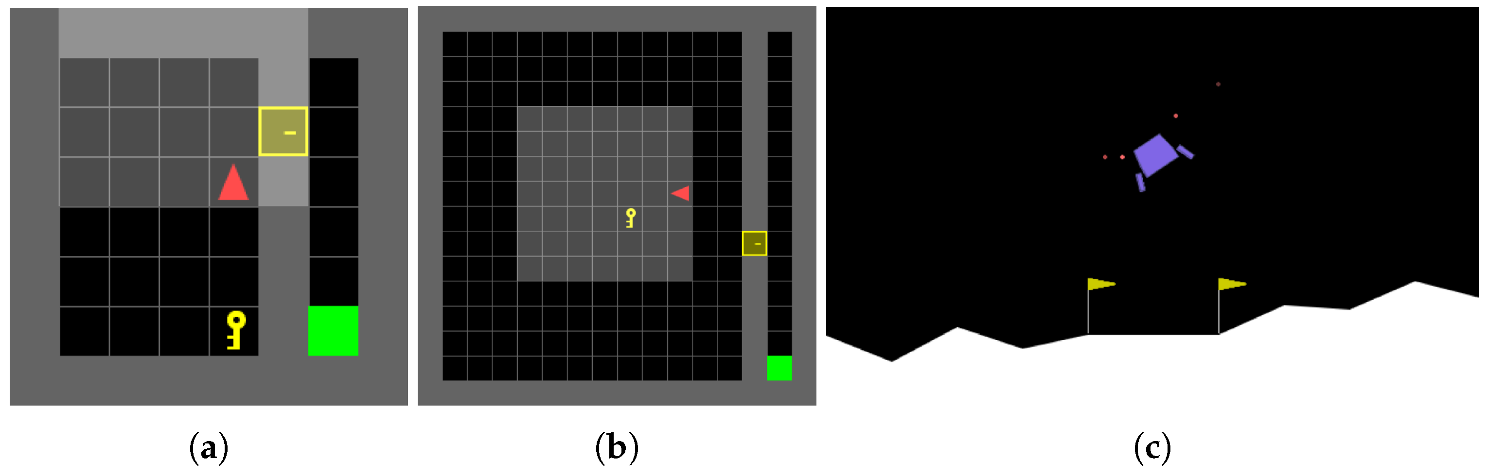
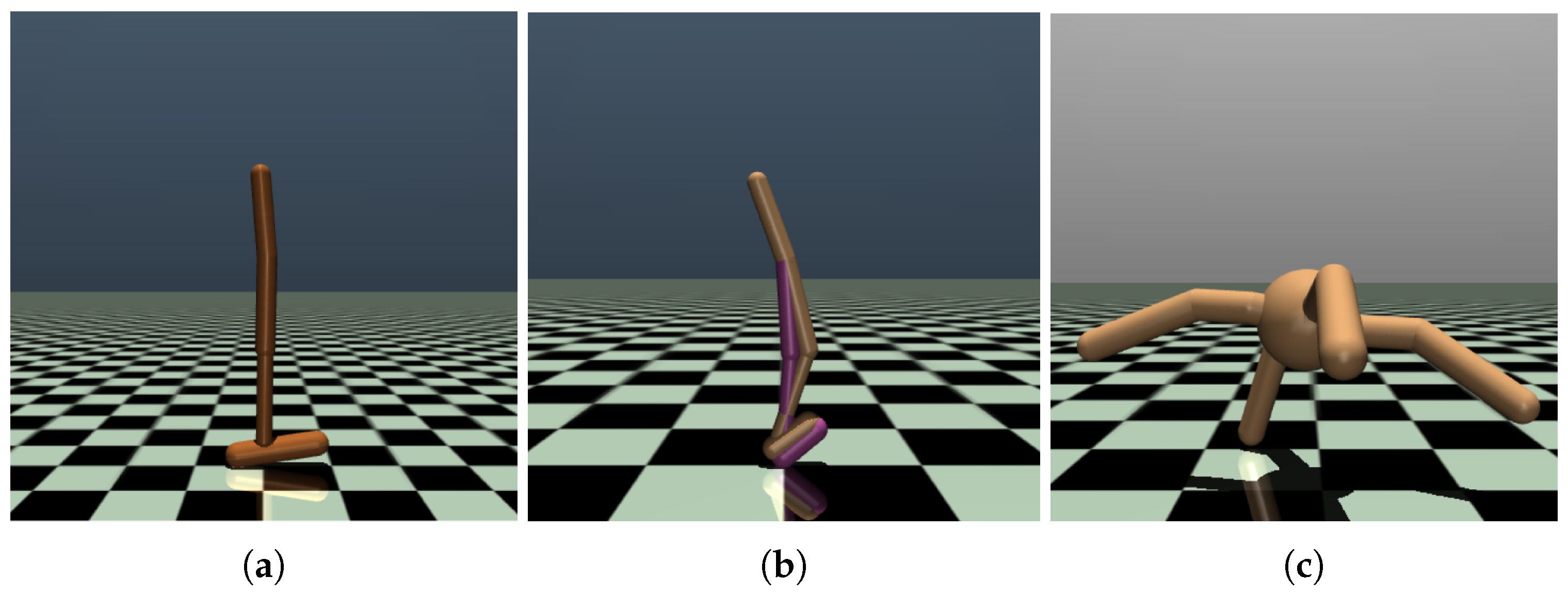
We conducted experiments in both discrete and continuous environments. The discrete environments are illustrated in Figure 8, including LunarLander [46] and MiniGrid-DoorKey [47]. The continuous environments are MuJoCo [48], including Walker2d, Hopper, and Ant, as illustrated in Figure 9. We adopted five distinct random seeds for each experimental setting and trained the model for 20,000 episodes under each seed configuration. The total reward and step count recorded in each episode were taken as the per-episode evaluation metrics. The final performance results were obtained by averaging the corresponding metric values across all five random seeds. Meanwhile, the raw experimental results were smoothed during post-processing. Specifically, the average value was calculated for every consecutive 50 episodes, and data points were sampled at an interval of 20 steps to generate the evaluation results presented for each episode. The experimental hyperparameters are listed in Table 1.

7.2. Distribution Analysis

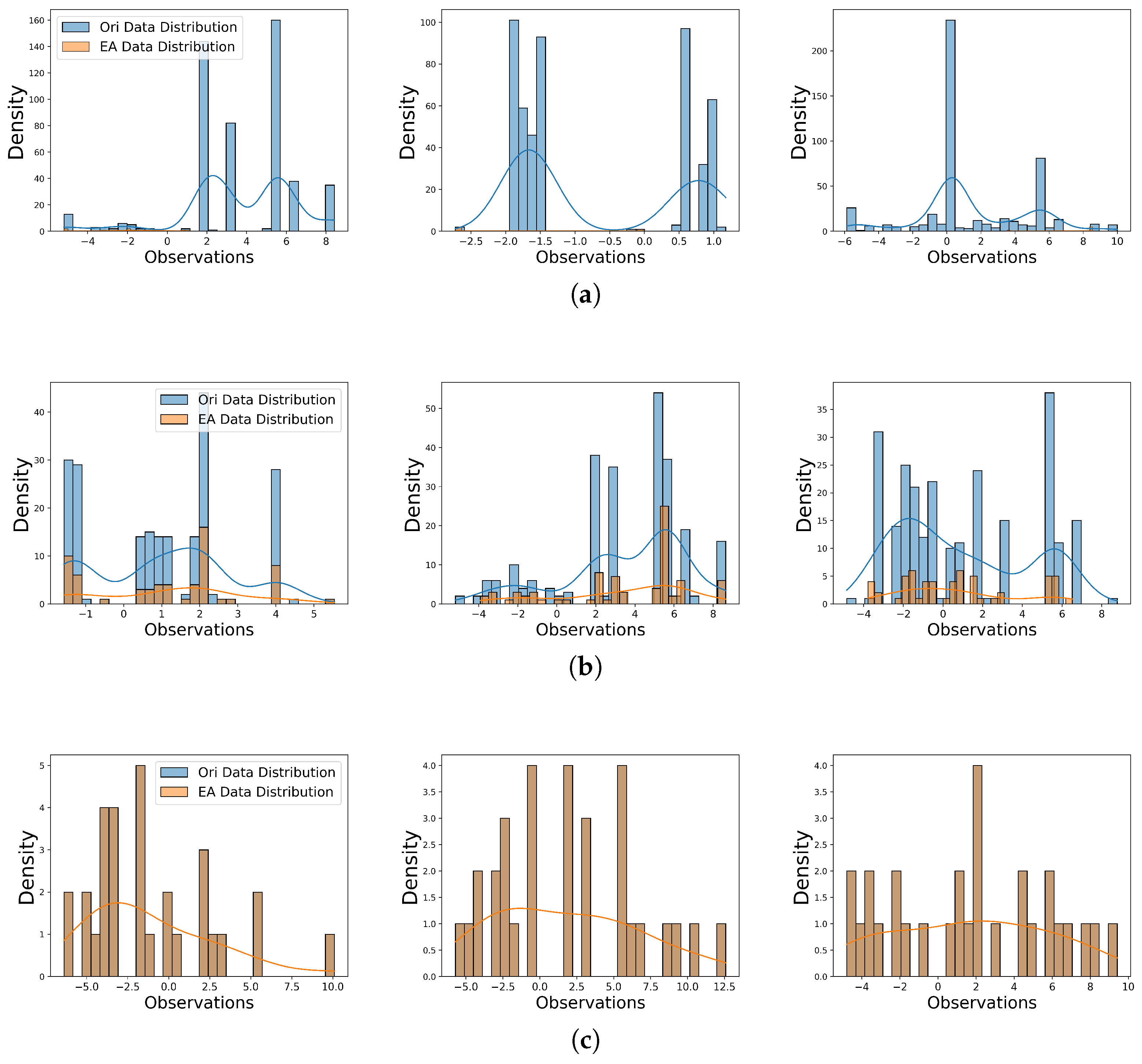
To provide a clear explanation of EATBEE, we visualize the τ and τ E A distributions using Principal Component Analysis (PCA), transforming the data from R d s to R . To enhance a comprehensive understanding of the tradeoff between exploration and exploitation using EATBEE, we selected three types of state data distributions: (1) exploration with task failure (Type 1)—the agent takes up to 500 steps but fails to complete the task; (2) exploration with task success (Type 2)—the agent takes more than 200 steps and successfully completes the task; (3) exploitation with task success (Type 3)—the agent takes 50 steps or fewer and completes the task. The data distributions of the trajectories are randomly selected, as illustrated in Figure 10.
In Type 1, the agent performs excessive exploration, and EATBEE filters out most of the exploratory data. In Type 2, the agent performs finite exploration and successfully completes the task, and EATBEE retains most of the exploitative data. In Type 3, the agent has fully completed the task, and EATBEE retains all sampled data. The visualization demonstrates that EATBEE dynamically adjusts the distribution of τ , achieving a tradeoff between exploration and exploitation.

7.3. Performance Evaluation of EATBEE

We compare EATBEE against the baseline algorithm (PPO). First, we introduce a selective indicator for EATBEE, termed Ratio, which quantifies the proportion between τ E A and τ :
R a t i o = E π [ | τ E A | ] E π [ | τ | ] .
where | · | represents the length of a sequence.
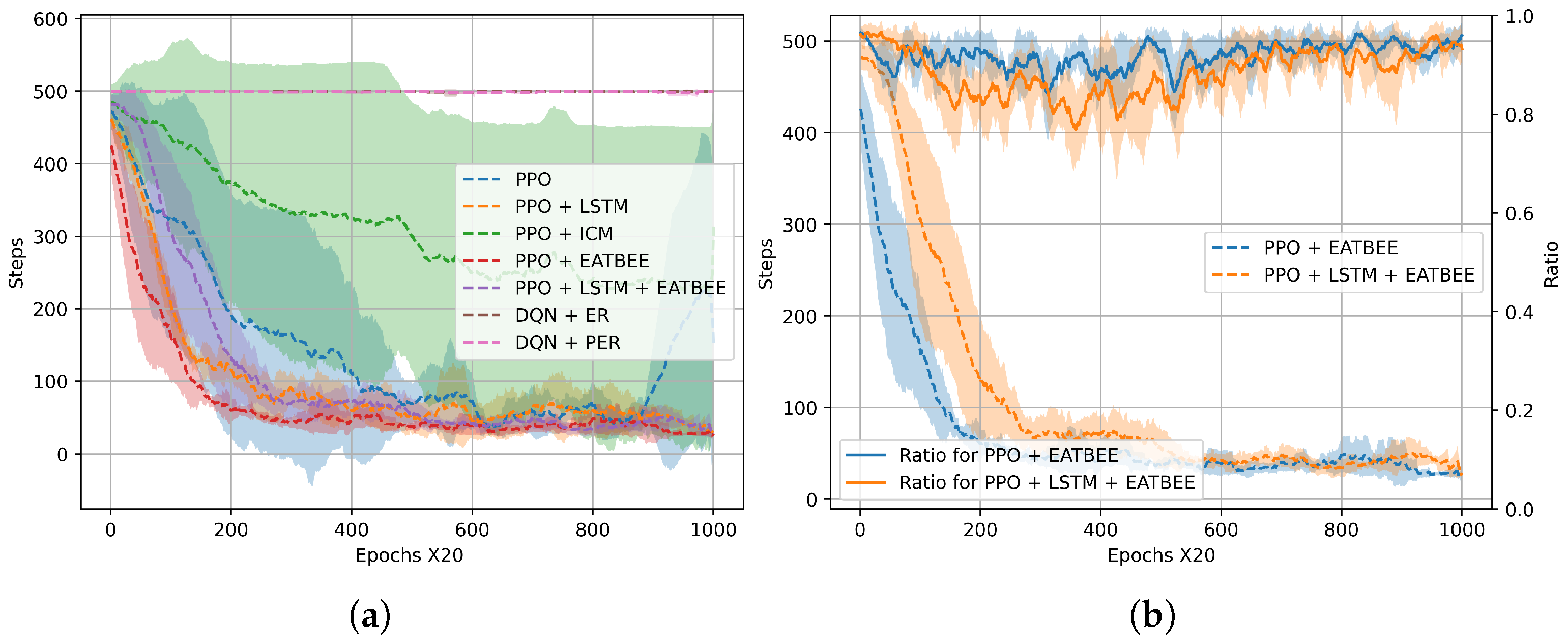
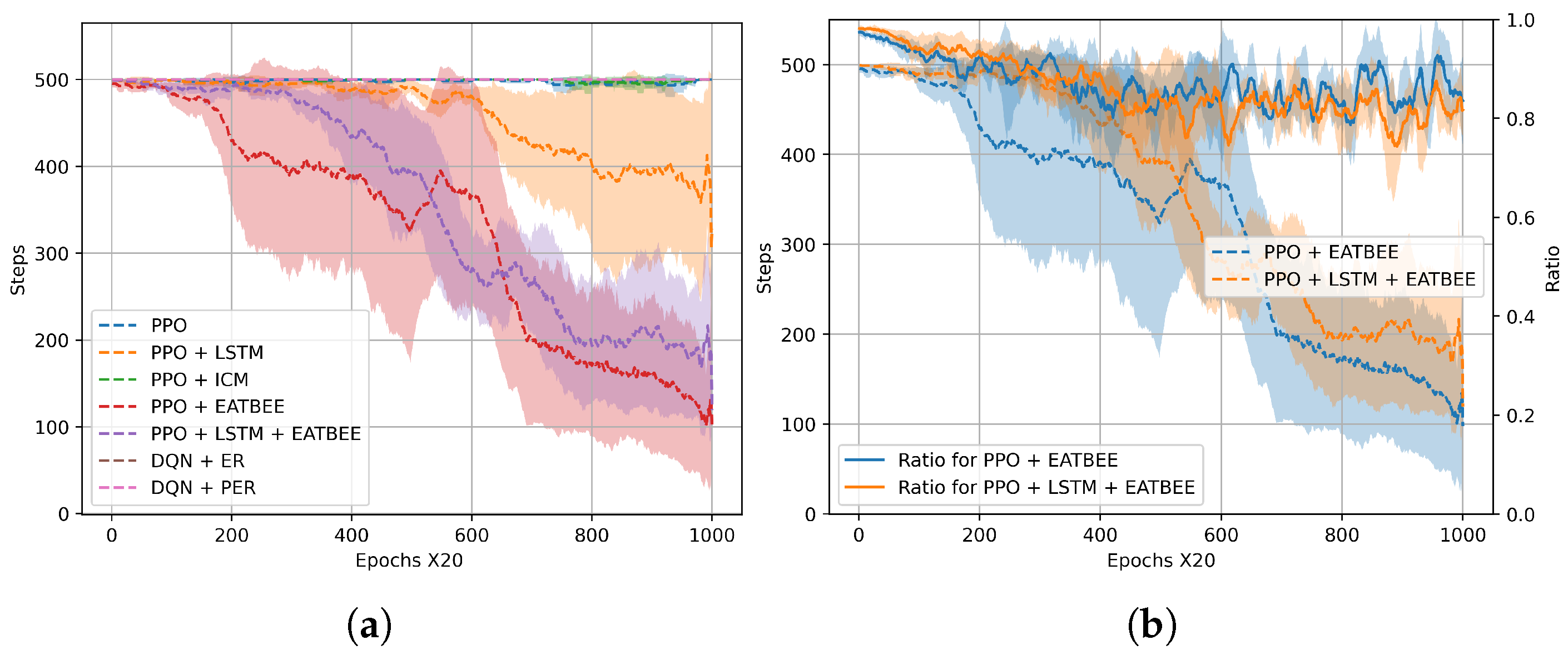
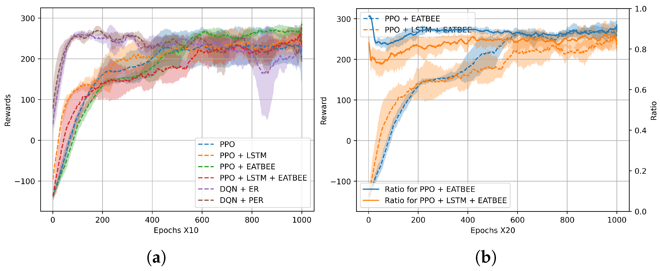
The performance of EATBEE in the MiniGrid-DoorKey-8 × 8 environment is illustrated in Figure 11 and Table 2. To further evaluate scalability and robustness, we extend the MiniGrid-DoorKey environment from an 8 × 8 grid to a more challenging 16 × 16 setting, and the results are illustrated in Figure 12 and Table 3. These results demonstrate that EATBEE achieves better performance and robustness than the baseline in sparse environments, which is consistent with the theoretical foundation of EATBEE. The experiment in a continuous state and discrete action environment, LunarLander, is illustrated in Figure 13 and Table 4. EATBEE autonomously discovers the knowledge necessary for the current policy.
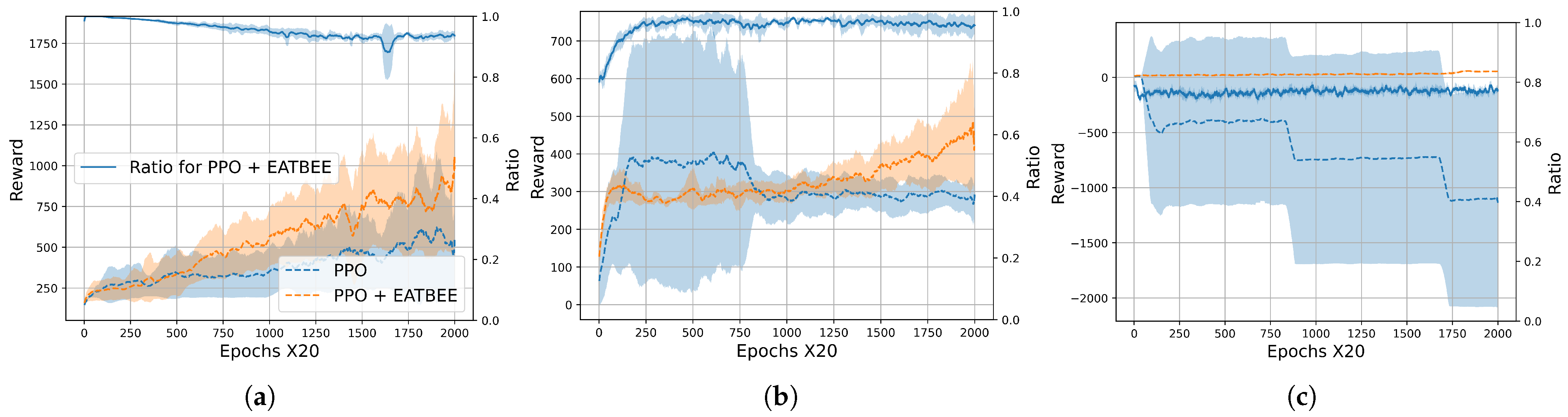
MuJoCo presents a significant challenge in continuous control due to its high-dimensional, continuous state and action spaces. We utilize MuJoCo benchmarks to validate that EATBEE can be combined with any algorithm and autonomously distill the essential knowledge for the current policy, with results shown in Figure 14 and Table 5.

8. Analysis of Transfer Learning in EATBEE

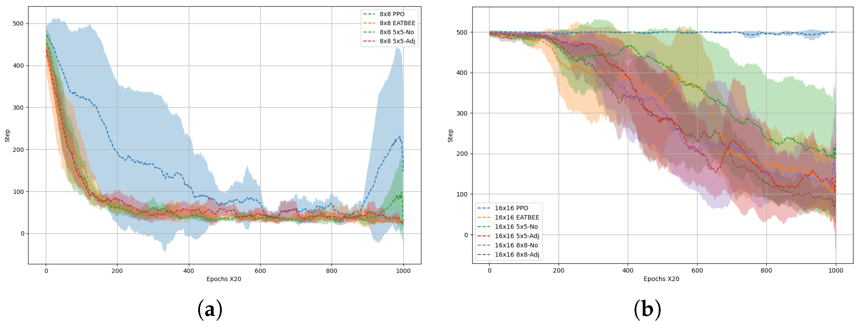
One of the key features of EATBEE is its ability to identify a data distribution that benefits the current policy from sampled data. A new question arises: in similar or identical task environments, does EATBEE have efficient transfer learning capabilities while still being able to screen environmental sampling data? We validated EATBEE’s transfer learning capability in the MiniGrid-DoorKey environment, as shown in Figure 15. First, we trained EATBEE in the MiniGrid-DoorKey-5 × 5 environment for 2000 epochs to ensure a thorough understanding of the task before progressing to experiments in the MiniGrid-DoorKey-8 × 8 and MiniGrid-DoorKey-16 × 16 environments. Due to the limited information available in the MiniGrid-DoorKey-5 × 5 environment, it is not feasible to fully understand the exploratory data distribution present in the MiniGrid-DoorKey-16 × 16 environment. Therefore, we carried out transfer learning experiments to obtain a converged EATBEE model specifically tailored for the MiniGrid-DoorKey-8 × 8 environment, which was subsequently applied successfully in the more complex MiniGrid-DoorKey-16 × 16 setting. The EATBEE migration consists of two types: fine-tuning and non-fine-tuning.

9. Ablation Experiment

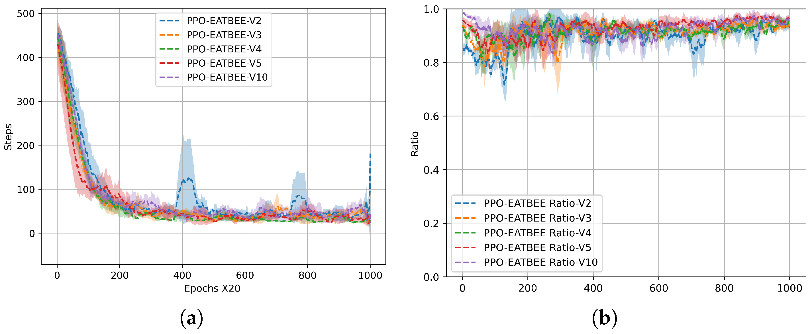
The approximated EATBEE comprises three core components: the number of state-value functions, the knowledge coefficient η , and the latent state space X . All experiments are conducted in the MiniGrid-DoorKey-8 × 8 environment, with all other experimental settings consistent with those employed in previous work. The state-value function serves as an alternative approach to calculating state similarity, while also encoding the inherent knowledge of the environment. The corresponding ablation results are presented in Figure 16. Experimental results show that increasing the number of state-value functions adopted in EATBEE improves the stability of its feature extraction performance. However, this increase does not bring about substantial improvements in overall performance. Notably, EATBEE can achieve satisfactory and effective data screening results when equipped with only two state-value functions.
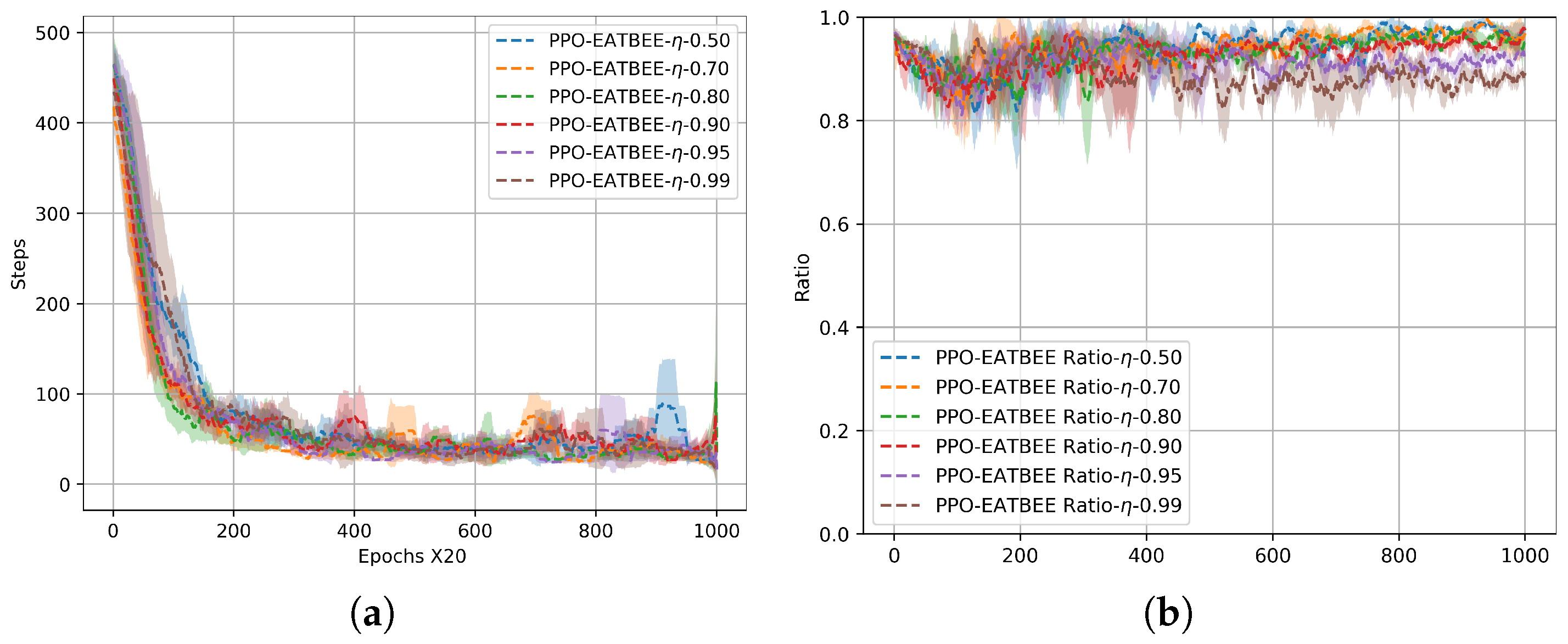
Another key component of EATBEE is the knowledge coefficient. This parameter determines the threshold and extent of environmental distribution knowledge captured by the EATBEE module. A higher value of η imposes stricter criteria for extracting environmental knowledge, while a lower η results in a more coarse-grained perception of environmental information. The knowledge coefficient, combined with the value function, jointly supports the measurement of state similarity. The ablation analysis of the knowledge coefficient η is presented in Figure 17. Experiments demonstrate that, with η = 0.99 , the EATBEE framework captures environmental knowledge in a more rigorous manner. After policy convergence and stabilization, the Ratio metric fails to approach 1. This outcome indicates that stable policy convergence in the MiniGrid-DoorKey-8 × 8 environment can be achieved without full data utilization. The present study attributes this phenomenon to the partial observability inherent to the aforementioned environment. During key retrieval and door-opening tasks, persistent exploratory behaviour remains necessary even after policy optimisation, which aligns with the inherent structural properties of the target environment. This finding validates that the environmental knowledge encoded by EATBEE is highly consistent with the actual characteristics of the physical environment.
As a core module of EATBEE, the latent space maintains the reachability of pruned states, which constitutes a fundamental premise of our method. In particular, any pruned state should still be reachable while satisfying the similarity constraint. We design ablation experiments to examine the role of the reachable latent space, and the outcomes are reported in Figure 18. The results verify that the reachable latent space is indispensable to the efficacy of EATBEE. If the reachability constraint across pruned states is broken, apparent discontinuities will appear in truncated trajectories. These abrupt fluctuations contradict the basic properties of Markov Decision Processes. Accordingly, reachability is a necessary condition to guarantee the valid application of the EATBEE framework.

10. Discussion

The proportion of exploration–exploitation data required by an agent differs substantially across distinct learning phases, yet agents lack the capability to identify these phases effectively. To tackle the challenge of agents failing to distinguish between exploration and exploitation data properly, this paper introduces the EATBEE method. The theoretical result shows that EATBEE achieves asymptotic monotonic improvement under well-defined assumptions, rather than strict monotonicity in all environments. Empirically, we validate that EATBEE’s phase-adaptive experience extraction mechanism contributes significantly to policy enhancement by aligning with the current stage of policy learning.
In comparison to existing studies on exploration and exploitation, EATBEE does not prioritize extensive state space exploration by the agent; instead, it implements efficient empirical data filtering to cater to the demands of the agent’s ongoing learning phase. Unlike research centered on experience replay techniques, EATBEE functions as a policy-adaptive data screening framework, rather than a uniform or post-hoc sampling mechanism, allowing it to accurately capture the specific data types required by the policy. Moreover, EATBEE offers strong interpretability, which is reflected in the clear comparative plots illustrating data distributions before and after raw data processing via EATBEE. In experiments spanning both discrete and continuous control tasks, EATBEE achieves performance levels comparable to the optimal results of baseline algorithms.
However, this study on EATBEE has certain limitations. For example, the current data extraction approach relies on correlation coefficients and value functions. Future research efforts can focus on advancing data screening strategies, aiming to develop a more intuitive data extraction method that can dynamically track the evolving needs of policy learning.

11. Conclusions

In existing RL algorithms, agents often exhibit over-exploration, resulting in slow policy convergence and instability. The reason is that existing algorithms cannot capture the knowledge within the data distribution. We introduced a sequential data extractor, EATBEE. First, we visualized the data distribution shift problem within a trajectory, and illustrated the extractor mechanism of EATBEE. Second, we built a theoretical guarantee for EATBEE to ensure monotonic policy improvement. Finally, through evaluation experiments, the results demonstrated that the EATBEE can autonomously extract the knowledge in most tasks and stabilize the policy learning. However, extracting relational data solely through correlation metrics poses certain inherent limitations; for instance, in continuous data regimes, temporally adjacent samples often exhibit excessively high similarity and may be erroneously discarded. Consequently, a pivotal direction for future inquiry lies in the development of more sophisticated extraction mechanisms that transcend elementary correlation-based filters.

Author Contributions

Writing—original draft preparation, Z.Y.; writing—review and editing, Z.W.; validation, Y.X.; visualization, M.C.; methodology, Y.D. All authors have read and agreed to the published version of the manuscript.

Funding

This work is supported in part by National Natural Science Foundation of China (No. 62306110), Key Research and Development Program of Hunan Province (No. 2024AQ2020), and Hunan Provincial Natural Science Foundation Project (No. 2025JJ80226).

Data Availability Statement

Data are contained within the article.

Conflicts of Interest

The authors declare no conflicts of interest.

Appendix A

Proof of Theorem 2. 
Suppose there are any two policies π and π , and
A π ( s , a ) = E s p ( · | s , a ) [ r ( s , a ) + γ V π ( s ) V π ( s ) ]
where r ( s , a ) is the immediate reward, V ( s ) is the state-value function, A ( s , a ) is the advantage function, and γ ( 0 γ 1 ) is the discount factor. Thus, the performance difference is
E τ P π ( τ ) [ t = 0 γ t A π ( s t , a t ) ] = E [ t = 0 γ t ( r ( s t , a t ) + γ V π ( s t + 1 ) V π ( s t ) ) ] = E [ V π ( s 0 ) + t = 0 γ t r ( s t , a t ) ] = E s 0 [ V π ( s 0 ) ] + E [ t = 0 γ t r ( s t , a t ) ] = J ( π ) J ( π ) = J ( π , π )
If J ( π , π ) > 0 is satisfied, then π has better performance than π , and vice versa.
Assuming a scenario with sparse rewards, we consider assigning a reward of r = 0 for each step and a reward of r T 0 for success or failure at the end. The objective of RL is to maximize the performance measure J ( θ ) :
J ( θ ) = E τ π ( τ ) [ G ( τ ) ] = δ E τ π ( τ ) [ G E A ( τ ) ] = δ J E A ( θ )
According to the Formula (6):
J ( π , π ) = J E A ( θ ) J ( θ ) = ( 1 δ ) J E A ( θ ) 0
where δ ( 0 , 1 ) . Therefore, J ( π , π ) > 0 must be satisfied. The policy π obtained from EATBEE-optimized data has better performance than the policy π obtained from the original data. □

References

  1. Ladosz, P.; Weng, L.; Kim, M.; Oh, H. Exploration in deep reinforcement learning: A survey. Inf. Fusion 2022, 85, 1–22. [Google Scholar] [CrossRef]
  2. Hao, J.; Yang, T.; Tang, H.; Bai, C.; Liu, J.; Meng, Z.; Liu, P.; Wang, Z. Exploration in deep reinforcement learning: From single-agent to multiagent domain. IEEE Trans. Neural Netw. Learn. Syst. 2023, 35, 8762–8782. [Google Scholar] [CrossRef]
  3. Huang, T.; Chen, K.; Li, B.; Liu, Y.H.; Dou, Q. Guided reinforcement learning with efficient exploration for task automation of surgical robot. In Proceedings of the 2023 IEEE International Conference on Robotics and Automation (ICRA); IEEE: Piscataway, NJ, USA, 2023; pp. 4640–4647. [Google Scholar]
  4. Matsuo, Y.; LeCun, Y.; Sahani, M.; Precup, D.; Silver, D.; Sugiyama, M.; Uchibe, E.; Morimoto, J. Deep learning, reinforcement learning, and world models. Neural Netw. 2022, 152, 267–275. [Google Scholar] [CrossRef]
  5. Ball, P.J.; Smith, L.; Kostrikov, I.; Levine, S. Efficient online reinforcement learning with offline data. In Proceedings of the 40th International Conference on Machine Learning, Honolulu, HI, USA, 23–29 July 2023; pp. 1577–1594. [Google Scholar]
  6. Bøhn, E.; Coates, E.M.; Reinhardt, D.; Johansen, T.A. Data-efficient deep reinforcement learning for attitude control of fixed-wing UAVs: Field experiments. IEEE Trans. Neural Netw. Learn. Syst. 2023, 35, 3168–3180. [Google Scholar] [CrossRef]
  7. Peng, Y.; Zeng, J.; Hu, Y.; Fang, Q.; Yin, Q. Reinforcement learning from suboptimal demonstrations based on Reward Relabeling. Expert Syst. Appl. 2024, 255, 124580. [Google Scholar] [CrossRef]
  8. Wang, Z.; Li, P.; Wang, Z.; Li, Z. Highway autonomous vehicle decision-making method based on prior knowledge and improved experience replay reinforcement learning algorithm. Expert Syst. Appl. 2025, 284, 127927. [Google Scholar] [CrossRef]
  9. Qin, P.; Zhao, T. Knowledge guided fuzzy deep reinforcement learning. Expert Syst. Appl. 2025, 264, 125823. [Google Scholar] [CrossRef]
  10. Zhang, H.; Dai, Y. A decomposition-based many-objective evolutionary algorithm with Q-learning guide weight vectors update. Expert Syst. Appl. 2025, 262, 125607. [Google Scholar] [CrossRef]
  11. Zhang, W.; Liu, J.; Li, L.; Liu, Y.; Wang, H. A knowledge driven two-stage co-evolutionary algorithm for constrained multi-objective optimization. Expert Syst. Appl. 2025, 274, 126908. [Google Scholar] [CrossRef]
  12. Pathak, D.; Agrawal, P.; Efros, A.A.; Darrell, T. Curiosity-driven exploration by self-supervised prediction. In Proceedings of the 34th International Conference on Machine Learning, Sydney, Australia, 6–11 August 2017; pp. 2778–2787. [Google Scholar]
  13. Burda, Y.; Edwards, H.; Storkey, A.; Klimov, O. Exploration by random network distillation. arXiv 2018, arXiv:1810.12894. [Google Scholar] [CrossRef]
  14. Chen, Z.; Zhao, Z.; Zhang, K.; Liu, B.; Qi, Q.; Wu, Y.; Kalluri, T.; Cao, S.; Xiong, Y.; Tong, H.; et al. Scaling Agent Learning via Experience Synthesis. arXiv 2025, arXiv:2511.03773. [Google Scholar] [CrossRef]
  15. Wang, H.; Su, A.; Ren, W.; Lin, F.; Chen, W. Pixel reasoner: Incentivizing pixel-space reasoning with curiosity-driven reinforcement learning. arXiv 2025, arXiv:2505.15966. [Google Scholar]
  16. Lobel, S.; Bagaria, A.; Konidaris, G. Flipping coins to estimate pseudocounts for exploration in reinforcement learning. In Proceedings of the 40th International Conference on Machine Learning, Honolulu, HI, USA, 23–29 July 2023; pp. 22594–22613. [Google Scholar]
  17. Wang, Y.; Zhao, K.; Liu, F.; U, L.H. Rethinking exploration in reinforcement learning with effective metric-based exploration bonus. Adv. Neural Inf. Process. Syst. 2024, 37, 57765–57792. [Google Scholar]
  18. Bai, C.; Zhang, Y.; Qiu, S.; Zhang, Q.; Xu, K.; Li, X. Online preference alignment for language models via count-based exploration. arXiv 2025, arXiv:2501.12735. [Google Scholar] [CrossRef]
  19. Seo, Y.; Chen, L.; Shin, J.; Lee, H.; Abbeel, P.; Lee, K. State entropy maximization with random encoders for efficient exploration. In Proceedings of the 38th International Conference on Machine Learning, Virtual, 18–24 July 2021; pp. 9443–9454. [Google Scholar]
  20. Yuan, M.; Pun, M.O.; Wang, D. Rényi state entropy maximization for exploration acceleration in reinforcement learning. IEEE Trans. Artif. Intell. 2022, 4, 1154–1164. [Google Scholar] [CrossRef]
  21. Kim, D.; Shin, J.; Abbeel, P.; Seo, Y. Accelerating reinforcement learning with value-conditional state entropy exploration. Adv. Neural Inf. Process. Syst. 2023, 36, 31811–31830. [Google Scholar]
  22. Burda, Y.; Edwards, H.; Pathak, D.; Storkey, A.; Darrell, T.; Efros, A.A. Large-scale study of curiosity-driven learning. arXiv 2018, arXiv:1808.04355. [Google Scholar]
  23. Reizinger, P.; Szemenyei, M. Attention-based curiosity-driven exploration in deep reinforcement learning. In Proceedings of the ICASSP 2020—2020 IEEE International Conference on Acoustics, Speech and Signal Processing (ICASSP); IEEE: Piscataway, NJ, USA, 2020; pp. 3542–3546. [Google Scholar]
  24. Chen, E.; Hong, Z.W.; Pajarinen, J.; Agrawal, P. Redeeming intrinsic rewards via constrained optimization. Adv. Neural Inf. Process. Syst. 2022, 35, 4996–5008. [Google Scholar]
  25. Kamuni, N.; Shah, H.; Chintala, S.; Kunchakuri, N.; Alla, S. Enhancing end-to-end multi-task dialogue systems: A study on intrinsic motivation reinforcement learning algorithms for improved training and adaptability. In Proceedings of the 2024 IEEE 18th International Conference on Semantic Computing (ICSC); IEEE: Piscataway, NJ, USA, 2024; pp. 335–340. [Google Scholar]
  26. Zhao, H.; Guo, Y.; Liu, Y.; Jin, J. Multirobot unknown environment exploration and obstacle avoidance based on a Voronoi diagram and reinforcement learning. Expert Syst. Appl. 2025, 264, 125900. [Google Scholar] [CrossRef]
  27. Daliri, A.; Alimoradi, M.; Zabihimayvan, M.; Sadeghi, R. World Hyper-Heuristic: A novel reinforcement learning approach for dynamic exploration and exploitation. Expert Syst. Appl. 2024, 244, 122931. [Google Scholar] [CrossRef]
  28. Fan, J.; Zhang, X.; Zou, Y. Hierarchical path planner for unknown space exploration using reinforcement learning-based intelligent frontier selection. Expert Syst. Appl. 2023, 230, 120630. [Google Scholar] [CrossRef]
  29. Hiraoka, T.; Onishi, T.; Wang, G.; Tsuruoka, Y. Which Experiences Are Influential for RL Agents? Efficiently Estimating The Influence of Experiences. In Proceedings of the Reinforcement Learning Conference, Edmonton, AB, Canada, 5–8 August 2025. [Google Scholar]
  30. Feng, S.; Sun, H.; Yan, X.; Zhu, H.; Zou, Z.; Shen, S.; Liu, H.X. Dense reinforcement learning for safety validation of autonomous vehicles. Nature 2023, 615, 620–627. [Google Scholar] [CrossRef]
  31. Mnih, V.; Kavukcuoglu, K.; Silver, D.; Rusu, A.A.; Veness, J.; Bellemare, M.G.; Graves, A.; Riedmiller, M.; Fidjeland, A.K.; Ostrovski, G.; et al. Human-level control through deep reinforcement learning. Nature 2015, 518, 529–533. [Google Scholar] [CrossRef]
  32. Zhang, T.; Guo, S.; Tan, T.; Hu, X.; Chen, F. Adjacency constraint for efficient hierarchical reinforcement learning. IEEE Trans. Pattern Anal. Mach. Intell. 2022, 45, 4152–4166. [Google Scholar] [CrossRef]
  33. Rother, D.; Weisswange, T.H.; Peters, J. Disentangling interaction using maximum entropy reinforcement learning in multi-agent systems. In ECAI 2023; IOS Press: Amsterdam, The Netherlands, 2023; pp. 1994–2001. [Google Scholar]
  34. Wang, Y.; Niu, Y.; Zhu, W.; Chen, W.; Li, Q.; Wang, T. Predicting pedestrian crossing behavior at unsignalized mid-block crosswalks using maximum entropy deep inverse reinforcement learning. IEEE Trans. Intell. Transp. Syst. 2023, 25, 3685–3698. [Google Scholar] [CrossRef]
  35. Li, T.; Zhu, K. Learning Joint Behaviors with Large Variations. In Proceedings of the 39th AAAI Conference on Artificial Intelligence, Philadelphia, PA, USA, 25 February–4 March 2025; Volume 39, pp. 23249–23257. [Google Scholar]
  36. Sukhija, B.; Coros, S.; Krause, A.; Abbeel, P.; Sferrazza, C. MaxInfoRL: Boosting exploration in reinforcement learning through information gain maximization. arXiv 2024, arXiv:2412.12098. [Google Scholar]
  37. Sancaktar, C.; Blaes, S.; Martius, G. Curious exploration via structured world models yields zero-shot object manipulation. Adv. Neural Inf. Process. Syst. 2022, 35, 24170–24183. [Google Scholar]
  38. Yuan, M.; Castanyer, R.C.; Li, B.; Jin, X.; Zeng, W.; Berseth, G. Rlexplore: Accelerating research in intrinsically-motivated reinforcement learning. arXiv 2024, arXiv:2405.19548. [Google Scholar]
  39. Yuan, M.; Zhang, Z.; Xu, Y.; Luo, S.; Li, B.; Jin, X.; Zeng, W. Rllte: Long-term evolution project of reinforcement learning. In Proceedings of the 39th AAAI Conference on Artificial Intelligence, Philadelphia, PA, USA, 25 February–4 March 2025; Volume 39, pp. 29718–29720. [Google Scholar]
  40. Yang, Q.; Spaan, M.T. Cem: Constrained entropy maximization for task-agnostic safe exploration. In Proceedings of the 37th AAAI Conference on Artificial Intelligence, Washington, DC, USA, 7–14 February 2023; Volume 37, pp. 10798–10806. [Google Scholar]
  41. Schaul, T.; Quan, J.; Antonoglou, I.; Silver, D. Prioritized Experience Replay. In Proceedings of the 4th International Conference on Learning Representations, San Juan, PR, USA, 2–4 May 2016. [Google Scholar]
  42. Yu, J.; Li, J.; Lü, S.; Han, S. Mixed experience sampling for off-policy reinforcement learning. Expert Syst. Appl. 2024, 251, 124017. [Google Scholar] [CrossRef]
  43. Kakade, S.; Langford, J. Approximately optimal approximate reinforcement learning. In Proceedings of the Nineteenth International Conference on Machine Learning, Sydney, Australia, 8–12 July 2002; pp. 267–274. [Google Scholar]
  44. Zhuang, Z.; Lei, K.; Liu, J.; Wang, D.; Guo, Y. Behavior Proximal Policy Optimization. In Proceedings of the Eleventh International Conference on Learning Representations, Kigali, Rwanda, 1–5 May 2023. [Google Scholar]
  45. Schulman, J.; Wolski, F.; Dhariwal, P.; Radford, A.; Klimov, O. Proximal policy optimization algorithms. arXiv 2017, arXiv:1707.06347. [Google Scholar] [CrossRef]
  46. Towers, M.; Kwiatkowski, A.; Balis, J.U.; Cola, G.D.; Deleu, T.; Goulão, M.; Andreas, K.; Krimmel, M.; KG, A.; Perez-Vicente, R.D.L.; et al. Gymnasium: A Standard Interface for Reinforcement Learning Environments. In Proceedings of the Thirty-Ninth Annual Conference on Neural Information Processing Systems Datasets and Benchmarks Track, San Diego, CA, USA, 2–7 December 2025. [Google Scholar]
  47. Chevalier-Boisvert, M.; Dai, B.; Towers, M.; Perez-Vicente, R.; Willems, L.; Lahlou, S.; Pal, S.; Castro, P.S.; Terry, J.K. Minigrid & miniworld: Modular & customizable reinforcement learning environments for goal-oriented tasks. Adv. Neural Inf. Process. Syst. 2023, 36, 73383–73394. [Google Scholar]
  48. Todorov, E.; Erez, T.; Tassa, Y. MuJoCo: A physics engine for model-based control. In Proceedings of the 2012 IEEE/RSJ International Conference on Intelligent Robots and Systems; IEEE: Piscataway, NJ, USA, 2012; pp. 5026–5033. [Google Scholar] [CrossRef]
  49. Kinga, D.; Adam, J.B. A method for stochastic optimization. In Proceedings of the 3rd International Conference on Learning Representations (ICLR), San Diego, CA, USA, 7–9 May 2015; Volume 5. [Google Scholar]
Figure 1. Conceptual framework of the Extractor for Adaptive Tradeoff Between Exploration and Exploitation (EATBEE) algorithm for correlation analysis and data quality enhancement within the latent adjacency matrix space. Black solid arrows represent the agent’s real trajectory transitions from the initial to the end state. Black dashed arrows denote the mapping and inverse mapping between the state and latent state spaces. Teal and red dashed arrows indicate latent state directions, with the red dashed arrow pointing to the interaction point between the real and ideal trajectories.
Mathematics 14 01624 g001
Figure 2. The optimal policy π * in a trajectory τ . Black solid arrows denote state transitions induced by the original policy π . Red solid arrows denote state transitions induced by the optimal policy π * . The red dashed arrow represents the skipped segment of the original trajectory, which is replaced by the optimal sub-trajectory. The original trajectory { s 0 , s 1 , , s T } is induced by the original sub-policy π 1 , whereas the optimal sub-trajectory { s 0 , , s i , s j + 1 , , s T } is induced by the optimal sub-policy π * , which skips the sub-sequence from s i + 1 to s j .
Mathematics 14 01624 g002
Figure 3. Backpropagation mechanism of EATBEE. Within the latent state space, EATBEE identifies a potentially optimal trajectory and updates the policy accordingly. The robot icon represents the agent interacting with the environment, and the red star denotes the target end state. Orange dots are original states in the state and latent spaces, green dots are newly identified potentially optimal states added via backpropagation, and the red dot is the central target state s x t in the latent space. Black solid arrows indicate state transitions in the original trajectory, while black dashed lines separate different processing stages. Red dashed arrows represent the encoding mapping s x = W ( s ) and decoding mapping s = M ( s x ) between the state space and latent state space. Orange dashed arrows show the temporal correspondence between trajectory states and the correlation matrix, and green curved arrows denote the backpropagation process that propagates optimal state information to update the policy. The color bar on the right represents the correlation coefficient between latent states (ranging from 0 to 1, with deeper blue indicating higher correlation).
Mathematics 14 01624 g003
Figure 4. The statistical mechanism of EATBEE. The light blue bars represent the original data distribution, and the light orange bars represent the optimized best data distribution. The brown bars denote the overlapping region between the two distributions, corresponding to the retained valid data that balances exploration and exploitation in the light exploration interval. The light blue and light orange smooth curves are the fitted density curves of the original and optimized distributions, respectively. The blue-labeled regions indicate overexploration segments where data deviates from the task goal. The red-bracketed regions mark the light exploration segments that balance exploration and exploitation, while the orange-bracketed region highlights the exploitation-focused data distribution driven by the task objective. When the agent explores excessively, EATBEE extracts exploitative transitions to improve policy learning.
Mathematics 14 01624 g004
Figure 5. The return G t E A ( τ ) for an excluded state s t . Black solid arrows denote the standard mapping from the original return G t ( τ ) to the filtered return G t E A ( τ ) for normally retained states. Black dashed arrows indicate the correspondence between original and filtered returns. Red solid and dashed arrows represent the special handling for the filtered state s t : the return G t ( τ ) is forced to 0, and its experience is excluded from the return calculation. The orange dashed box highlights the processing unit of the filtered state s t . When s t is filtered out by EATBEE, G t E A ( τ ) is set to 0.
Mathematics 14 01624 g005
Figure 6. The operational mechanism of EATBEE. The blue horizontal line separates the two trajectory groups: the top row shows the optimal trajectory refined by EATBEE, while the bottom row shows the raw execution of the original trajectory. Black curved arrows labeled “Optimal Path” denote the progression of the optimized trajectory across steps. Green solid arrows labeled “Efficient Backpropagation” indicate the direction of the efficient backpropagation process that propagates optimal information backward. Orange bidirectional arrows show the correspondence between steps in the original and optimized trajectories. Red dashed boxes highlight redundant steps in the original trajectory that are eliminated by EATBEE. In each game frame, the blue triangle represents the agent, the light blue symbols represent the key and door respectively, and the green square indicates the terminal state. The original trajectory comprises 225 steps, which is significantly reduced to 27 steps following EATBEE optimization. Both the current and total step counts are displayed in the upper-left corner of each frame.
Mathematics 14 01624 g006
Figure 7. Consistency and monotonicity analysis of value functions: EATBEE vs. original trajectories. Black curved arrows labeled “Optimal Path” denote the progression of the optimized trajectory across steps. Green solid arrows labeled “Efficient Backpropagation” indicate the direction of the efficient backpropagation process that propagates optimal information backward. Orange bidirectional arrows show the correspondence between steps in the original and optimized trajectories. In each game frame, the blue triangle represents the agent, the light blue symbols represent the key and door respectively, and the green square indicates the terminal state. In the original sequence (bottom), the agent transitions through numerous redundant states (e.g., from step 2 to 20). EATBEE identifies these as low-information segments and refines them into an optimized trajectory (top). Crucially, the labels V t V t E A and V t E A V t + 1 E A indicate that state-value estimates remain stable and monotonically increasing despite the removal of intermediate steps. This confirms that the extractor effectively preserves the task-relevant knowledge distribution.
Mathematics 14 01624 g007
Figure 8. Environments with discrete actions. (a) MiniGrid-DoorKey-8 × 8: In each game frame, the red triangle represents the agent, the yellow symbols represent the key and door respectively, and the green square indicates the terminal state. A small grid-world environment with sparse rewards, where the agent must collect a key, open the door, and reach the goal state. (b) MiniGrid-DoorKey- 16 × 16 : A larger-scale variant of the DoorKey task with increased complexity. (c) LunarLander: A continuous control environment with dense rewards, where the agent controls a lander to safely land between two flags.
Mathematics 14 01624 g008
Figure 9. Environments with continuous actions. The agent needs to keep walking and must not fall down. (a) Hopper: A single-leg hopping environment where the agent controls a single articulated leg to maintain balance and move forward. (b) Walker2d: A two-legged walking environment where the agent controls two legs (purple for the left leg, brown for the right leg) to achieve stable forward locomotion. (c) Ant: A four-legged ant-like environment with higher-dimensional continuous action space, requiring coordinated control of all legs to move forward.
Mathematics 14 01624 g009
Figure 10. Visualization of data distribution for different trajectory types. (a) Type 1: exploration with task failure. (b) Type 2: exploration with task success. (c) Type 3: exploitation with task success. The horizontal axis represents the state embedding after Principal Component Analysis (PCA) projection (from R d s to R ), and the vertical axis represents density. The blue bars and corresponding blue solid Kernel Density Estimation (KDE) curve show the distribution of the original trajectory τ , while the orange bars and corresponding orange solid KDE curve show the distribution of the EATBEE-filtered trajectory τ E A .
Mathematics 14 01624 g010
Figure 11. Evaluations in the MiniGrid-DoorKey-8 × 8 environment. (a) The EATBEE performance. (b) The Ratio between exploration and exploitation. Detailed hyperparameter configurations for both Proximal Policy Optimization (PPO) and Deep Q-Network (DQN) are summarized in Table 1. In our benchmarks, PPO + Long Short-Term Memory (LSTM) denotes the PPO algorithm integrated with an LSTM network, while PPO + Intrinsic Curiosity Module (ICM) and PPO + EATBEE refer to PPO augmented with the ICM and our proposed EATBEE module, respectively. Regarding the DQN baselines, DQN + Experience Replay (ER) represents the vanilla DQN equipped with ER and a target network, whereas DQN + Prioritized Experience Replay (PER) denotes the variant incorporating PER.
Mathematics 14 01624 g011
Figure 12. EATBEE performance in the MiniGrid-DoorKey-16 × 16 environment. (a) The EATBEE performance. (b) The Ratio between exploration and exploitation.
Mathematics 14 01624 g012
Figure 13. EATBEE performance in the LunarLander environment. (a) The EATBEE performance. (b) The Ratio between exploration and exploitation.
Mathematics 14 01624 g013
Figure 14. EATBEE performance in MuJoCo environment. (a) Hopper. (b) Walker2d. (c) Ant.
Mathematics 14 01624 g014
Figure 15. The analysis of transfer learning using EATBEE in the MiniGrid-DoorKey environment. (a) The transfer learning in MiniGrid-DoorKey-8 × 8 for EATBEE. (b) The transfer learning in MiniGrid-DoorKey-16 × 16 for EATBEE. The EATBEE approach does not focus on a specific policy but rather on the data distribution of the task, making it highly adaptable to similar or identical tasks. The following symbols are explained: 8 × 8 PPO refers to the MiniGrid-DoorKey-8 × 8 environment using PPO; 8 × 8 EATBEE refers to the MiniGrid-DoorKey-8 × 8 environment using PPO with EATBEE; 8 × 8 5 × 5-no refers to using the converged PPO with EATBEE from the 5 × 5 environment without updating the EATBEE network in the MiniGrid-DoorKey-8 × 8 environment; and, finally, 8 × 8 5 × 5-adj refers to using the converged PPO with the EATBEE module from the 5 × 5 environment while updating the EATBEE network in an 8 × 8 MiniGrid-DoorKey setting. In a MiniGrid-DoorKey-16 × 16 scenario, transfer learning with EATBEE carries the same significance.
Mathematics 14 01624 g015
Figure 16. Ablation experiments on state-value functions. (a) Number of state-value functions. (b) The Ratio between exploration and exploitation. Symbol explanation: V2 denotes the use of two state-value functions. As the number of state-value functions increases, EATBEE exhibits enhanced capability in data filtering, leading to more stable overall policy performance. For instance, PPO-EATBEE-V5 and -V10 demonstrate smaller standard deviations, with the final Ratio metric approaching 1.
Mathematics 14 01624 g016
Figure 17. Ablation experiments on the knowledge coefficient. (a) Size of knowledge coefficient η . (b) The Ratio between exploration and exploitation. As this coefficient increases, EATBEE consistently guarantees stable convergence of RL algorithms. The Ratio results reveal that a larger knowledge coefficient enables stricter capture of environmental knowledge distribution. For tasks requiring precise modeling of environmental knowledge patterns, a relatively large value of η is recommended.
Mathematics 14 01624 g017
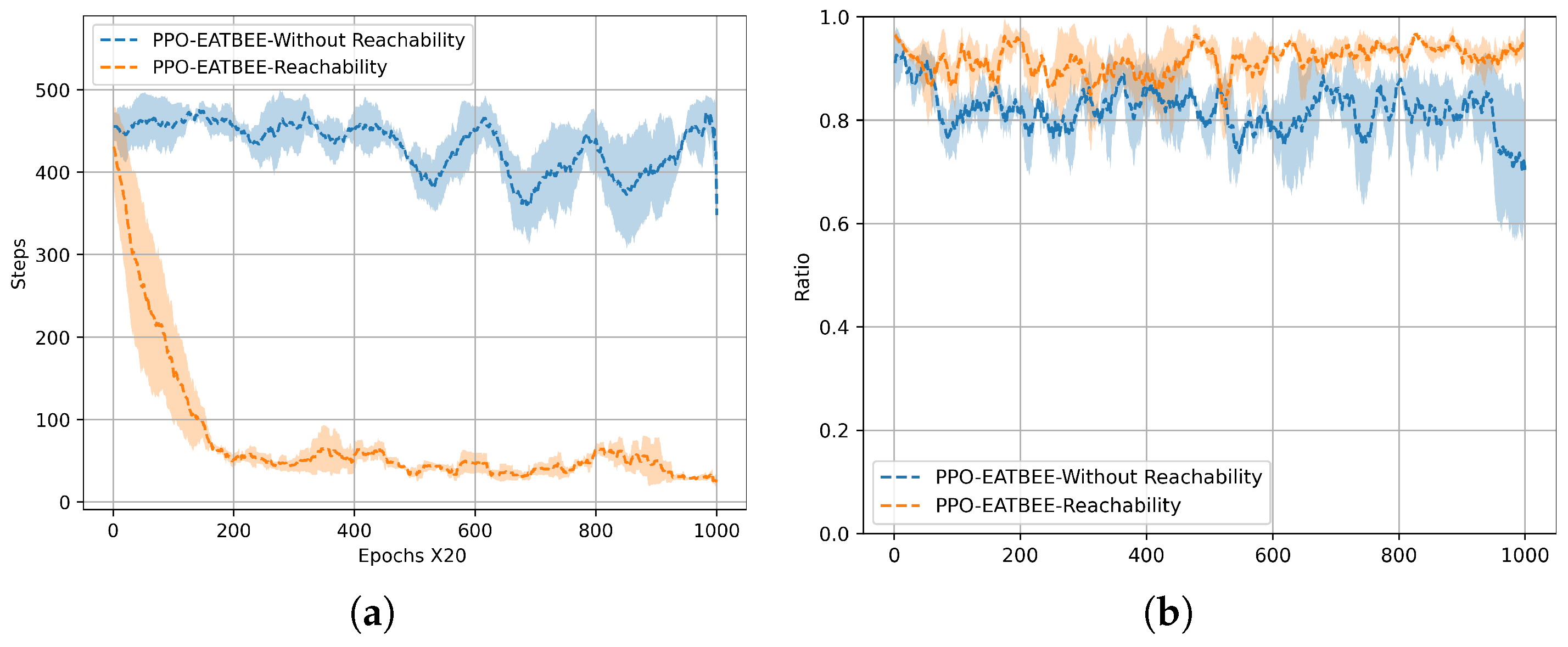
Figure 18. Ablation experiments on reachability. (a) Latent Space and Reachability Effects. (b) The Ratio between exploration and exploitation. When reachability within the latent space is compromised, EATBEE loses rigorous constraints during data filtering. This issue introduces abrupt jumps in pruned trajectory data, weakening the model’s capacity to capture environmental knowledge. Consequently, the RL algorithm fails to learn from valid, high-quality samples.
Mathematics 14 01624 g018
Table 1. Hyperparameter details.
PPODQN
OptimizerAdam [49]Adam
learning rate 3 × 10 4 3 × 10 4
discount ( γ ) 0.99 0.99
Replay Buffer SizeNone 1 × 10 6
Number of Hidden Layers22
Number of Hidden Units Per Layer6464
Number of Samples Per MinibatchNone256
NonlinearityReLUReLU
Table 2. The performance comparison in the MiniGrid-DoorKey-8 × 8 environment.
Min StepMax Step10% MS20% MS30% MS40% MS50% MS
PPO 15.2 ± 2.48 500 134.12 ± 123.44 93.69 ± 58.24 80.27 ± 40.03 75.75 ± 31.48 74.62 ± 27.38
PPO + LSTM 15.2 ± 3.66 500 43.81 ± 4.17 47.44 ± 6.69 50.12 ± 11.5 50.40 ± 13.85 52.18 ± 18.13
PPO + ICM 143.4 ± 180.72 500 229.47 ± 220.91 232.66 ± 218.53 242.38 ± 211.11 242.94 ± 210.63 251.11 ± 204.80
PPO + EATBEE 14.8 ± 1.72 500 35 . 68 ± 8 . 45 37 . 53 ± 8 . 98 37 . 50 ± 6 . 25 37 . 62 ± 6 . 89 38 . 14 ± 6 . 80
PPO + LSTM + EATBEE 14 . 6 ± 3 . 38 500 41.74 ± 7.40 39.37 ± 4.62 40.27 ± 4.68 40.49 ± 3.78 42.49 ± 3.83
DQN + ER 412.0 ± 176.0 500 499.86 ± 0.28 499.85 ± 0.28 499.83 ± 0.32 499.84 ± 0.30 499.84 ± 0.30
DQN + PER 413.8 ± 172.4 500 499.39 ± 0.91 499.43 ± 0.82 499.39 ± 0.88 499.39 ± 0.89 499.43 ± 0.83
Table 3. The performance comparison in the MiniGrid-DoorKey-16 × 16 environment.
Min StepMax Step10% MS20% MS30% MS40% MS50% MS
PPO339.4 ± 198.52500496.47 ± 4.63496.89 ± 3.28496.77 ± 2.55497.42 ± 2.05497.79 ± 1.71
PPO + LSTM 175.6 ± 163.00 500 388.34 ± 95.81 393.83 ± 96.07 403.21 ± 86.66 418.68 ± 70.56 431.58 ± 56.64
PPO + ICM 406.0 ± 188.00 500 497.95 ± 4.07 497.46 ± 5.07 497.96 ± 4.08 498.47 ± 3.06 498.77 ± 2.45
PPO + EATBEE 39.4 ± 7.00 500 143 . 38 ± 75 . 64 153 . 08 ± 79 . 78 167 . 46 ± 77 . 97 204 . 89 ± 69 . 16 235 . 32 ± 69 . 23
PPO + LSTM + EATBEE 39 . 0 ± 14 . 46 500 195.48 ± 68.74 201.83 ± 71.43 213.34 ± 65.39 234.57 ± 54.09 259.54 ± 40.23
DQN + ER426.2 ± 147.6500499.86 ± 0.28500.0 ± 0.0500 ± 0.0500 ± 0.0500 ± 0.0
DQN + PER448.2 ± 103.60500499.98 ± 0.05499.99 ± 0.03499.99 ± 0.02499.99 ± 0.02499.99 ± 0.01
Table 4. The performance comparison in the LunarLander environment.
Min RewardMax Reward10% MR20% MR30% MR40% MR50% MR
PPO−314.42 ± 101.27290.33 ± 23.22230.98 ± 42.04231.10 ± 42.77231.19 ± 43.22230.71 ± 43.78229.61 ± 43.92
PPO + LSTM 365.62 ± 70.73 302.93 ± 16.86 235.54 ± 28.65 234.37 ± 30.91 234.86 ± 30.64 232.62 ± 30.88 230.34 ± 29.68
PPO + EATBEE 302 . 37 ± 122 . 28 307 . 87 ± 20 . 62 263 . 49 ± 2 . 90 264 . 06 ± 2 . 03 262 . 04 ± 3 . 58 260 . 54 ± 5 . 79 255 . 87 ± 7 . 73
PPO + LSTM + EATBEE 343.17 ± 132.99 300.16 ± 7.06 235.72 ± 11.95 229.14 ± 16.48 224.4 ± 17.07 221.19 ± 17.75 213.9 ± 19.82
DQN + ER−538.21 ± 1313.68291.78 ± 9.14108.86 ± 93.92120.17 ± 99.12141.25 ± 86.89155.61 ± 72.13156.20 ± 57.56
DQN + PER−787.09 ± 1244.59287.51 ± 13.34−78.10 ± 111.93−57.22 ± 67.68−54.24 ± 49.29−47.92 ± 39.76−37.41 ± 36.66
Table 5. The performance comparison in MuJoCo.
Min RewardMax Reward10% MR20% MR30% MR40% MR50% MR
PPO-Hopper10.42 ± 3.411001.86 ± 981.75555.89 ± 353.09520.14 ± 302.63506.22 ± 282.70484.76 ± 260.26463.50 ± 231.01
PPO + EATBEE-Hopper 14 . 22 ± 3 . 93 1849 . 49 ± 1195 . 62 823 . 12 ± 342 . 79 798 . 23 ± 313 . 54 773 . 11 ± 304 . 48 747 . 69 ± 283 . 99 718 . 53 ± 264 . 58
PPO-Walker−7.71 ± 9.17612.83 ± 450.23291.29 ± 41.78289.34 ± 43.31289.58 ± 43.20290.96 ± 43.87290.74 ± 46.67
PPO + EATBEE-Walker 5 . 64 ± 15 . 87 738 . 39 ± 454 . 81 420 . 80 ± 99 . 10 404 . 77 ± 85 . 38 388 . 16 ± 73 . 98 374 . 49 ± 64 . 83 362 . 23 ± 55 . 61
PPO-Ant−1183.82 ± 872.4566.14 ± 46.72−1103.86 ± 975.20−982.08 ± 898.34−897.62 ± 883.52−857.43 ± 888.60−834.28 ± 894.73
PPO + EATBEE-Ant 68 . 00 ± 106 . 60 137 . 78 ± 67 . 84 54 . 88 ± 1 . 43 44 . 48 ± 2 . 27 39 . 84 ± 2 . 13 37 . 31 ± 2 . 34 35 . 34 ± 2 . 50
Disclaimer/Publisher’s Note: The statements, opinions and data contained in all publications are solely those of the individual author(s) and contributor(s) and not of MDPI and/or the editor(s). MDPI and/or the editor(s) disclaim responsibility for any injury to people or property resulting from any ideas, methods, instructions or products referred to in the content.