On Graphs with Maximal Sum of α-th Degree Powers

Abstract

Let G be a simple graph. The sum of the $\alpha$-th degree powers of G, denoted by $M_{\alpha }\left(G\right)$, is obtained by summing the $\alpha$-th powers of all vertex degrees. We use ${\mathfrak{G}}_{n,m}$ to denote the set of all graphs having n vertices and m edges. Extremal problems concerning $M_2\left(G\right)$ have a long history in combinatorics and graph theory. In 1971, Katz (Israel J. Math., 1971) first initiated the study of maximizing $M_2\left(G\right)$ within ${\mathfrak{G}}_{n,m}$. After nearly 40 years, Ábrego et al. (J. Inequal. Pure and Appl. Math., 2009) completely resolved this problem. In this paper, we extend the power exponent from $\alpha =2$ to $\alpha >2$, investigating the problem of determining the graph that maximizes the value of $M_{\alpha }\left(G\right)$ within ${\mathfrak{G}}_{n,m}$. We show that the graph that maximizes $M_{\alpha }\left(G\right)$ when $\alpha >2$ and $1\le m\le {\displaystyle \frac{1}{4}}\left({\displaystyle \genfrac{}{}{0pt}{}{n}{2}}\right)$ is the quasi-star graph, which belongs to a special class of threshold graphs (defined in the Introduction).

1. Introduction

All graphs considered in this paper are finite, simple, and undirected. For standard graph-theoretic notation and terminology, the reader is referred to [1].

We use ${\mathfrak{G}}_{n,m}$ to denote the set of all $(n,m)$-graphs, in which each of them has n vertices and m edges. Let $G=(V,E)$ be a simple graph with order n and degree sequence $(d_1,d_2,\dots ,d_n)$. For a positive real $\alpha$, the $\alpha$-th degree power is defined as

$$M_{\alpha }=M_{\alpha }\left(G\right)={\displaystyle \sum _{i=1}^n}{d}_i^{\alpha }.$$

The investigation of degree-based topological indices originated in chemical graph theory to characterize molecular structures. The first Zagreb index, introduced by Gutman and Trinajstić in 1972 [2], is defined as the sum of squared vertex degrees, namely $M_2\left(G\right)$. Initially applied to approximate the total $\pi$-electron energy of alternant hydrocarbons, this index has been established as a fundamental topological invariant. Subsequently, this index was generalized to the general zeroth-order Randić index, also known as the variable first Zagreb index, by allowing an arbitrary real exponent $\alpha$. The development and applications of degree-based topological indices are surveyed by Ali et al. [3] and Gutman [4,5]; Furtula and Gutman [6] studied the related forgotten topological index, Li and Zheng [7] developed a unified approach to extremal trees for several degree-based indices, and Todeschini and Consonni [8] introduced local vertex invariants based on degree functions. The introduction of an exponent $\alpha >2$ is tailored for the precise characterization of extreme hub polarization (i.e., super-nodes) and asymmetric branching phenomena within complex networks and chemical macromolecules.

The maximization of the degree power sum $M_{\alpha }\left(G\right)$ has been extensively studied in extremal graph theory [9]. For the quadratic case $\alpha =2$, Katz [10] and Ahlswede–Katona [11] pioneered the maximization problem over the family of $(n,m)$-graphs, whose combinatorial objective algebraically translates to maximizing the number of incident edge pairs. Subsequently, Olpp [12] constructed two families of extremal threshold graphs, formally establishing that maximizing $M_2\left(G\right)$ is structurally equivalent to maximizing the total number of (not necessarily induced) paths of length two. This structural landscape was further refined independently by Peled, Petreschi, and Sterbini [13], and by Byer [14], who constrained the set of all $M_2\left(G\right)$-optimal graphs to exactly six specific subclasses of threshold graphs. Ultimately, Ábrego et al. [15] provided a complete resolution to this quadratic extremal problem. The main difficulty in passing from $\alpha =2$ to $\alpha \ne 2$ is that the diagonal sequence ceases to be a complete invariant for the objective function.

For $0<\alpha <1$, the minimum value of $M_{\alpha }\left(G\right)$ was characterized by Linial–Rozenman [16] and Ismailescu–Stefanica [17]. When $\alpha \ge 2$ and $m\le n-2$, Ismailescu–Stefanica [17] described the maximizers among all $(n,m)$-graphs; Zhang–Zhang [18] recently pushed the range to $m\le 2n-3$. Up to now, the case for $\alpha >2$ has remained open.

While the general maximization over $(n,m)$-graphs for $\alpha >2$ remains elusive, significant progress has been made by shifting the focus toward restricted graph families and alternative structural parameters. For instance, in the realm of Turán-type extremal problems, Ai et al. [19] determined the maximum $M_{\alpha }\left(G\right)$ for $P_k$-free graphs when $\alpha \ge 2$, rigorously compressing the critical order lower bound to a linear size of $O\left(k\right)$. From a graph transformation perspective, Cheng and Wu [20] established strict inequality bounds between a connected graph and its line graph across three distinct parameter intervals: $\alpha \ge 1$, $0<\alpha <1$, and $\alpha \le -1$. Furthermore, by incorporating specific invariant constraints, Vetrík et al. [21] completely characterized the exact upper and lower bounds of $M_{\alpha }\left(G\right)$ for trees with a given distance k-domination number across all non-trivial ranges ($\alpha >1$, $0<\alpha <1$, and $\alpha <0$), identifying all corresponding extremal structures.

A graph G is defined as a threshold graph if it is $\{2K_2,C_4,P_4\}$-free. Threshold graphs form a well-studied class; their structural properties and equivalent characterizations are summarized in the monograph of Mahadev and Peled [22]. They also arise naturally as extremal graphs in several settings, including the maximization of adjacent edge pairs [11], network reliability problems [23], extremal homomorphism counts [24,25], the minimization of the number of matchings [26], and problems involving randomly deleted edges [27]. Within this broader class, our analysis specifically targets two highly structured subclasses: quasi-complete graphs and quasi-star graphs. Let A and B be two disjoint graphs. Denote by $A\cup B$ the sum of A and B, where $V(A\cup B)=V\left(A\right)\cup V\left(B\right)$ and $E(A\cup B)=E\left(A\right)\cup E\left(B\right)$. Denote by $A\vee B$, the $join$ of A and B, the graph obtained from $A\cup B$ by adding all the edges $(u,h)$ with $u\in V\left(A\right)$ and $h\in V\left(B\right)$. The graph $C_{n,m}:=(K_{k-j}\vee (K_1\cup K_j))\cup (n-k-1)K_1$ is referred to as quasi-complete, where k and j are integers and are uniquely determined by the expression

$$m=\left({\displaystyle \genfrac{}{}{0pt}{}{k+1}{2}}\right)-j,1\le j\le k\le n-1.$$

(1)

The graph $S_{n,m}:=K_{n-k^{\prime }-1}\vee ((K_1\vee j^{\prime }{K}_1)\cup (k^{\prime }-j^{\prime })K_1)$ is referred to as quasi-star, where $k^{\prime }$, $j^{\prime }$ are integers and are uniquely determined by the expression

$$m=\left({\displaystyle \genfrac{}{}{0pt}{}{n}{2}}\right)-\left({\displaystyle \genfrac{}{}{0pt}{}{k^{\prime }+1}{2}}\right)+j^{\prime },1\le j^{\prime }\le k^{\prime }\le n-1.$$

(2)

Both quasi-star and quasi-complete graphs are often extremal graphs for some graph invariants (see, e.g., [28]).

For instance, when $(n,m)=(7,9)$, the quasi-complete graph is determined by

$$9=\left({\displaystyle \genfrac{}{}{0pt}{}{5}{2}}\right)-1,$$

so $k=4$ and $j=1$. Hence,

$$C_{7,9}=\left(K_3\vee (K_1\cup K_1)\right)\cup 2K_1,$$

which is $K_5$ with one edge removed, together with two isolated vertices. On the other hand, the quasi-star graph is determined by

$$9=\left({\displaystyle \genfrac{}{}{0pt}{}{7}{2}}\right)-\left({\displaystyle \genfrac{}{}{0pt}{}{6}{2}}\right)+3,$$

so $k^{\prime }=5$ and $j^{\prime }=3$, and

$$S_{7,9}=K_1\vee \left((K_1\vee 3K_1)\cup 2K_1\right).$$

For convenience, we refer to a graph G as an α-optimal $(n,m)$-graph if

$$M_{\alpha }\left(G\right)=max\{M_{\alpha }\left(H\right):H\in {\mathfrak{G}}_{n,m}\}.$$

In this paper, we consider the following problem:

Problem 1. 

For $\alpha >2$, can we determine all α-optimal graphs within ${\mathfrak{G}}_{n,m}$?

For $\alpha >2$, each $\alpha$-optimal $(n,m)$-graph is a threshold graph (see, e.g., [15] (p. 5)), hence it suffices to consider threshold graphs. Using an algebraic method, we refer to each Ferrers matrix of a threshold graph as a weight matrix such that each entry within the matrix is assigned a weight that quantifies its contribution to the global degree power sum $M_{\alpha }\left(G\right)$.

Theorem 1. 

Let $\alpha >2$ and G be an α-optimal $(n,m)$-graph. Then G is quasi-star if

$$1\le m\le {\displaystyle \frac{1}{4}}\left({\displaystyle \genfrac{}{}{0pt}{}{n}{2}}\right).$$

We briefly outline the proof strategy. After reducing the problem to threshold graphs, we represent an optimal graph by its Ferrers matrix and assign weights to the black dots. Thus, maximizing $M_{\alpha }\left(G\right)$ becomes equivalent to maximizing the total weight of the matrix. For $\alpha >2$, strict convexity allows us to compare dot weights and use weight-increasing swapping operations. These operations, combined with a counting argument, show that every optimal graph is quasi-star in the range $1\le m\le {\displaystyle \frac{1}{4}}\left({\displaystyle \genfrac{}{}{0pt}{}{n}{2}}\right)$.

The remainder of this paper is organized as follows. In Section 2, we introduce necessary preliminaries, including the Ferrers matrix representation of threshold graphs and essential analytical properties of strictly convex functions. In Section 3, we establish a series of lemmas based on the corner-swapping operation on the Ferrers matrix. Utilizing these algebraic tools, we conclude by presenting the proof of Theorem 1.

2. Preliminaries

In this section, we will introduce the notation and terminology that will be utilized in the subsequent discussion.

Let G be an n-vertex threshold graph. During its step-by-step construction, a newly added vertex v is isolated if it connects to no previously existing vertices, and dominating if it connects to all previously existing vertices. Structurally, any threshold graph of order n can be constructed by successively adjoining either an isolated or a dominating vertex. Consequently, the structure of a threshold graph can be canonically encoded by a binary sequence of length n. Specifically, we associate a threshold graph with a sequence $\sigma \in {\{0,1\}}^n$, where the entry ${\sigma }_i=0$ indicates the addition of an isolated vertex $v_i$, and ${\sigma }_i=1$ indicates the addition of a dominating vertex $v_i$. By convention, the initial vertex $v_1$ is assigned ${\sigma }_1=0$,

$$(\underset{a_1}{\underbrace{0\dots 0}}\underset{b_1}{\underbrace{1\dots 1}}\dots \underset{a_k}{\underbrace{0\dots 0}}\underset{b_k}{\underbrace{1\dots 1}})=(0^{a_1}{1}^{b_1}\dots 0^{a_k}{1}^{b_k}),$$

where all exponent runs $a_i$ and $b_i$ are strictly positive integers, with the sole exception of $b_k$, which is permitted to be zero in the case of a disconnected graph. For simplification, we replace the above binary representation with the vector $(a_1,\dots ,a_k;b_1,\dots ,b_k)$ and refer to it as the vertex-sequence of such a threshold graph.

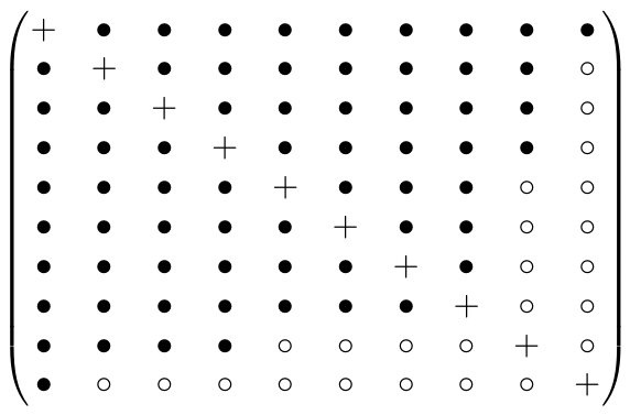
To systematically analyze the structural properties of threshold graphs, we employ the Ferrers matrix representation. Let G be a threshold graph with a non-increasing degree sequence $d=(d_1,d_2,\dots ,d_n)$. The corresponding Ferrers matrix $F={\left(f_{ij}\right)}_{n\times n}$ is a symbolic matrix whose entries are drawn from the alphabet $\{\circ ,•,+\}$. The configuration of these entries is strictly governed by the following rules (see [22]):

• All diagonal elements $f_{ii}$, $i=1,\dots ,n$, are +;
• For each i, the sum of the “•” in the i-th row is equal to $d_i$;
• Each “•” in each row is to the left.

By construction, the Ferrers matrix of a threshold graph is necessarily symmetric. It therefore suffices to restrict our analysis to the strictly lower triangular region. Specifically, configuring the Ferrers matrix for a threshold graph with m edges is combinatorially equivalent to determining a valid placement of exactly m symbols • below the main diagonal. An example of a Ferrers matrix is shown in Figure 1.

Let $F={\left(f_{ij}\right)}_{n\times n}$ denote the Ferrers diagram of a threshold graph G. Within the area below the main diagonal, we identify specific boundary points that determine the valid transformations of the matrix:

1.

A coordinate $(i,j)$ with $n\ge i>j\ge 1$ is defined as an outer corner if it is currently occupied ($f_{i,j}=•$), yet strictly bounded by non-occupied cells to its right ($f_{i,j+1}\ne •$) and below ($f_{i+1,j}=\circ$, or $i=n$).

2.

A coordinate $(p,q)$ with $n\ge p>q\ge 1$ is defined as an inner corner if it is currently vacant ($f_{p,q}=\circ$), yet immediately shielded by occupied or diagonal cells from above ($f_{p-1,q}\in \{+,•\}$) and from the left ($f_{p,q-1}=•$, or $q=1$).

Furthermore, let $F+st$ (respectively, $F-st$) represent the updated configuration obtained from F by toggling the state of the entry $(s,t)$ (and, by symmetry, $(t,s)$) from ∘ to • (respectively, from • to ∘). It is a direct structural consequence that $F+st$ remains a valid Ferrers diagram if $(s,t)$ is an inner corner, and $F-st$ remains valid if $(s,t)$ is an outer corner.

In addition, we need to introduce some basic facts about the convexity of functions.

Definition 1. 

Let $f:I\to \mathbb{R}$ be a function defined on an interval $I\subset \mathbb{R}$.

• $f\left(x\right)$ is called convex on I if for all $x_1,x_2\in I$ and all $\lambda \in [0,1]$,

  $$f(\lambda x_1+(1-\lambda )x_2)\le \lambda f\left(x_1\right)+(1-\lambda )f\left(x_2\right).$$

  It is called strictly convex on I if the above inequality is strict whenever $x_1\ne x_2$ and $\lambda \in (0,1)$.

Lemma 1 

([29]). Let $f\left(x\right)$ be a function on the interval I. Then $f\left(x\right)$ is convex on I if and only if for all $x_1,x_2\in I$ with $x_1<x_2$ and all $x\in (x_1,x_2)$,

$${\displaystyle \frac{f\left(x\right)-f\left(x_1\right)}{x-x_1}}\le {\displaystyle \frac{f\left(x_2\right)-f\left(x_1\right)}{x_2-x_1}}\le {\displaystyle \frac{f\left(x_2\right)-f\left(x\right)}{x_2-x}}.$$

Moreover, $f\left(x\right)$ is strictly convex on I if and only if the two inequalities are strict for every triple $x_1<x<x_2$.

As a consequence of Lemma 1, we have

Corollary 1. 

Let $t>0$ and $f\left(x\right)$ be a function on the interval I. If $f\left(x\right)$ is strictly convex on I, then for all $i,j\in I$ with $j\le i$ and $j-t,i+t\in I$,

$$f(i+t)-f\left(i\right)-f\left(j\right)+f(j-t)>0.$$

Proof. 

For a convex function $f\left(x\right)$, if $j-t<j<i<i+t$, by Lemma 1, we have

$${\displaystyle \frac{f\left(j\right)-f(j-t)}{j-(j-t)}}<{\displaystyle \frac{f\left(i\right)-f\left(j\right)}{i-j}}<{\displaystyle \frac{f(i+t)-f\left(i\right)}{i+t-i}}.$$

Thus,

$$f\left(j\right)-f(j-t)<f(i+t)-f\left(i\right).$$

If $i-t<i=j<i+t$, by Lemma 1, we have

$${\displaystyle \frac{f\left(i\right)-f(i-t)}{i-(i-t)}}<{\displaystyle \frac{f(i+t)-f\left(i\right)}{(i+t)-i}}.$$

Thus,

$$f\left(i\right)-f(i-t)<f(i+t)-f\left(i\right),$$

which is equivalent to

$$f(i+t)-2f\left(i\right)+f(i-t)>0.$$

The result follows. □

Theorem 2 

([15] (p. 5)). Let α be an arbitrary real number with $\alpha \ge 2$. Then each α-optimal graph in ${\mathfrak{G}}_{n,m}$ is a threshold graph.

3. Main Results

This section characterizes optimal graphs via Ferrers matrices. By symmetry, it strictly suffices to investigate the arrangement of solid dots solely below the main diagonal.

Lemma 2. 

Let $\alpha >2$ and G be a threshold graph with Ferrers matrix F. If $(i,j),i>j$ is an inner corner of F, then

$$M_{\alpha }\left(G^{*}\right)-M_{\alpha }\left(G\right)={(i-1)}^{\alpha }-{(i-2)}^{\alpha }+j^{\alpha }-{(j-1)}^{\alpha },$$

where $G^{*}$ denotes the graph whose Ferrers matrix is obtained from F by changing the entry $f_{ij}$ from an empty dot to a black dot.

Proof. 

Let $V\left(G\right)=\{1,2,\dots ,n\}$. Suppose that, for each i, the vertex i corresponds to the i-th row and the i-th column of F. Since $(i,j)$ is an inner corner, it follows that $d_{G^{*}}\left(i\right)=d_G\left(i\right)+1=j$ and $d_{G^{*}}\left(j\right)=d_G\left(j\right)+1=i-1$ and $d_{G^{*}}\left(x\right)=d_G\left(x\right)$ if $x\notin \{i,j\}$. Then, we have

$$M_{\alpha }\left(G^{*}\right)-M_{\alpha }\left(G\right)=\sum _{w\in V\left(G^{*}\right)}{\left(d_{G^{*}}\left(w\right)\right)}^{\alpha }-\sum _{w\in V\left(G\right)}{\left(d_G\left(w\right)\right)}^{\alpha }={(i-1)}^{\alpha }-{(i-2)}^{\alpha }+j^{\alpha }-{(j-1)}^{\alpha }.$$

Thus, the proof is complete. □

We know that each threshold graph within ${\mathfrak{G}}_{n,m}$ can be obtained by successively adding m edges to an empty graph with n vertices. Since the threshold graph G has a one-to-one correspondence to its Ferrers matrix F, the problem of characterizing the $\alpha$-optimal graph within ${\mathfrak{G}}_{n,m}$ can be reduced to that of constructing an appropriate Ferrers matrix with m black dots in its lower triangular part by Lemma 2. Therefore, we define the weight of a Ferrers matrix as follows. Let F be the Ferrers matrix corresponding to some threshold graph G, we define

$$w_{ij}^{\alpha }=\left\{\begin{array}{cc}{(i-1)}^{\alpha }-{(i-2)}^{\alpha }+j^{\alpha }-{(j-1)}^{\alpha },\hfill & \mathrm{if}{f}_{ij}=“•”\mathrm{and}n\ge i>j\ge 1;\hfill \\ 0,\hfill & \mathrm{otherwise},\hfill \end{array}\right.$$

and

$$W_{\alpha }\left(F\right)=\sum _{i>j\ge 1}{w}_{ij}^{\alpha }.$$

(3)

As a consequence of Lemma 2, we have

Theorem 3. 

Let $\alpha >2$ and G be a threshold graph with Ferrers matrix F. Then

$$M_{\alpha }\left(G\right)=W_{\alpha }\left(F\right),$$

where $W_{\alpha }\left(F\right)$ is defined as Equation (3).

Proof. 

We proceed by induction on m. If $m=0$, then G is empty and $M_{\alpha }\left(G\right)=W_{\alpha }\left(F\right)=0$. Assume the statement holds for all threshold graphs with $m-1$ edges. Let G be a threshold graph with m edges and Ferrers matrix F. Deleting one edge (the edge corresponding to one outer corner) yields a threshold graph $G^{\prime }$ with Ferrers matrix $F^{\prime }$ obtained from F by replacing “•” at position $(i,j)$ with “∘”. Only the degrees of i and j change:

$$d_i\left(G\right)=d_i\left(G^{\prime }\right)+1,d_j\left(G\right)=d_j\left(G^{\prime }\right)+1.$$

For a Ferrers matrix of a threshold graph,

$$d_i\left(G^{\prime }\right)=j-1,d_j\left(G^{\prime }\right)=i-2,$$

hence

$$\begin{array}{ccc}\hfill M_{\alpha }\left(G\right)-M_{\alpha }\left(G^{\prime }\right)& =& {(i-1)}^{\alpha }-{(i-2)}^{\alpha }+j^{\alpha }-{(j-1)}^{\alpha }=w_{ij}^{\alpha }.\hfill \end{array}$$

Since $(i,j)$ is the only “•” of F missing in $F^{\prime }$,

$$W_{\alpha }\left(F\right)=W_{\alpha }\left(F^{\prime }\right)+w_{ij}^{\alpha }.$$

Therefore, by the induction hypothesis, it follows that

$$M_{\alpha }\left(G\right)=M_{\alpha }\left(G^{\prime }\right)+w_{ij}^{\alpha }=W_{\alpha }\left(F^{\prime }\right)+w_{ij}^{\alpha }=W_{\alpha }\left(F\right),$$

where the induction hypothesis is used in the second equality. □

Example 1. 

We give an example to illustrate the weighted Ferrers-matrix method. Consider the threshold graph with vertex-sequence

$$(a_1,a_2;b_1,b_2)=(3,1;2,0).$$

Equivalently, this graph is obtained by adding three isolated vertices, then two dominating vertices, and finally one isolated vertex. Its non-increasing degree sequence is

$$(4,4,2,2,2,0),$$

and its Ferrers matrix is

$$F=\left(\begin{array}{cccccc}+& •& •& •& •& \circ \\ •& +& •& •& •& \circ \\ •& •& +& \circ & \circ & \circ \\ •& •& \circ & +& \circ & \circ \\ •& •& \circ & \circ & +& \circ \\ \circ & \circ & \circ & \circ & \circ & +\end{array}\right).$$

There are seven black dots below the main diagonal, and hence the corresponding graph has seven edges.

The entry $(5,2)$ is an outer corner dot, since

$$f_{5,2}=“•”,f_{5,3}=“\circ ”,f_{6,2}=“\circ ”.$$

The entry $(6,1)$ is an inner corner position, since

$$f_{6,1}=“\circ ”,f_{5,1}=“•”,$$

and it is in the first column.

For a lower-triangular entry $(i,j)$, the weight is

$$w_{ij}^{\alpha }={(i-1)}^{\alpha }-{(i-2)}^{\alpha }+j^{\alpha }-{(j-1)}^{\alpha }.$$

Thus $w_{5,2}^{\alpha }=4^{\alpha }-3^{\alpha }+2^{\alpha }-1,$ whereas $w_{6,1}^{\alpha }=5^{\alpha }-4^{\alpha }+1.$ For example, when $\alpha =3$, $w_{5,2}^3=4^3-3^3+2^3-1^3=44,$ and $w_{6,1}^3=5^3-4^3+1^3-0^3=62.$ Hence, replacing the outer corner dot $(5,2)$ by the inner corner position $(6,1)$ increases the total weight by 18.

After this corner transformation, the Ferrers matrix becomes

$$F^{\prime }=\left(\begin{array}{cccccc}+& •& •& •& •& •\\ •& +& •& •& \circ & \circ \\ •& •& +& \circ & \circ & \circ \\ •& •& \circ & +& \circ & \circ \\ •& \circ & \circ & \circ & +& \circ \\ •& \circ & \circ & \circ & \circ & +\end{array}\right).$$

The number of black dots below the diagonal is still seven, so the number of edges is preserved. The degree sequence changes from $(4,4,2,2,2,0)$ to $(5,3,2,2,1,1).$ For $\alpha =3$, the value of $M_{\alpha }$ changes from

$$4^3+4^3+3·2^3=152$$

to

$$5^3+3^3+2·2^3+2·1^3=170.$$

Thus, the corner transformation increases $M_3$ by 18, exactly the increase predicted by the weight difference

$$w_{6,1}^3-w_{5,2}^3=18.$$

This example illustrates the basic principle used in the proofs below: a Ferrers matrix cannot be optimal if some outer corner dots can be replaced by the same number of inner corner positions with strictly larger total weight.

To construct our desired Ferrers matrix, we need to establish a series of lemmas.

Lemma 3. 

Let $\alpha >2$ and F be a Ferrers matrix. Let also $f_{ij}=f_{pq}=$“•” $withi>j\ge 1andp>q\ge 1.$ Then

(1) 

$w_{ij}^{\alpha }>w_{pq}^{\alpha }$ if $i=p$ and $j>q$;

(2) 

$w_{ij}^{\alpha }>w_{pq}^{\alpha }$ if $j=q$ and $i>p$;.

(3) 

for $i+j=p+q$ and $i>p$, $w_{ij}^{\alpha }>w_{pq}^{\alpha }$.

Proof. 

Let $g(x;\alpha )=x^{\alpha }-{(x-1)}^{\alpha }$. Then we have

$$w_{ij}^{\alpha }=g(i-1;\alpha )+g(j;\alpha )\mathrm{and}{w}_{pq}^{\alpha }=g(p-1;\alpha )+g(q;\alpha ).$$

Thus, (1) and (2) follow by a direct verification.

(3) If $i+j=p+q$ and $i>p$, then we get $i>p>q>j$. Moreover, one can verify that $g(x;\alpha )$ is strictly convex if $\alpha >2.$ Consequently, applying Corollary 1, the result follows. □

Lemma 4. 

Let $\alpha >2$ and G be an α-optimal graph within ${\mathfrak{G}}_{n,m}$. Suppose that the vertex-sequence of G is $(a_1,\dots ,a_k;b_1,\dots ,b_k),$ $k\ge 2.$ Then either $b_i=1$ or $b_i>a_i$ for $i=1,\dots ,k-1$.

Proof. 

Denote by $F={\left(f_{ij}\right)}_{n\times n}$ the Ferrers matrix of G. Assume for contradiction that there exists some index $i(1\le i\le k-1)$ such that $1<b_i\le a_i$. For simplification, set ${\sum }_{j=1}^k{b}_j+{\sum }_{t=1}^i{a}_t=x$ and ${\sum }_{j=i+1}^k{b}_j=y$. Then one can verify that the entry $(x+1,y+1)$ is an inner corner and the entry $(x,y+b_i)$ is an outer corner of F, respectively. Denote by $F^{*}$ the matrix obtained from F by changing $b_i-1$ entries $(x-b_i+1+t,y+b_i)$, $t=1,\dots ,b_i-1$, from “$•$” to “$\circ$”, and changing $b_i-1$ entries $(x+1,y+t)$, $t=1,\dots ,b_i-1$, from “$\circ$” to “$•$”. One can find that the matrix $F^{*}$ is also a Ferrers matrix of some threshold graph, denoted by $G^{*}$, within ${\mathfrak{G}}_{n,m}$. Applying Lemma 3 (3), $w_{x+1,y+t}^{\alpha }>w_{x-b_i+1+t,y+b_i}^{\alpha }$ holds for each $t(t=1,\dots ,b_i-1)$. Consequently,

$$W_{\alpha }\left(F^{*}\right)>W_{\alpha }\left(F\right),$$

which is a contradiction to the optimality of the graph G. Therefore, the result follows. □

Lemma 5. 

Let $\alpha >2$ and G be an α-optimal graph within ${\mathfrak{G}}_{n,m}$. Suppose that the vertex-sequence of G is $(a_1,\dots ,a_k;b_1,\dots ,b_k),$ $k\ge 2$. Then, for each $i(i=1,\dots ,k-1)$, either $b_i=1$ or $b_i>a_i+a_{i+1}$.

Proof. 

Denote by $F={\left(f_{ij}\right)}_{n\times n}$ the Ferrers matrix of G. Assume for contradiction that there exists some index i, $1\le i\le k-1$, such that $a_i<b_i\le a_i+a_{i+1}$, as $b_i>a_i$ if $b_i\ne 1$ by Lemma 4. So we get $b_i-a_i>0.$ For simplification, set ${\sum }_{j=1}^k{b}_j+{\sum }_{t=1}^i{a}_t=x$ and ${\sum }_{j=i+1}^k{b}_j=y$. Denote by $F^{*}$ the matrix obtained from F by changing $a_i(b_i-a_i)$ entries $(x-a_i+t,y+a_i+s)$ from “$•$” to “$\circ$”, and changing $a_i(b_i-a_i)$ entries $(x+s,y+t)$ from “$\circ$” to “$•$”, where $t=1,\dots ,a_i$ and $s=1,\dots ,b_i-a_i$. One can find that the matrix $F^{*}$ is also a Ferrers matrix of some threshold graph, denoted by $G^{*}$, in ${\mathfrak{G}}_{n,m}$. Applying Lemma 3 (3),

$$w_{x+s,y+t}^{\alpha }>w_{x-a_i+t,y+a_i+s}^{\alpha }$$

holds for each pair $(s,t)$, where $t=1,\dots ,a_i$ and $s=1,\dots ,b_i-a_i$. Consequently,

$$W_{\alpha }\left(F^{*}\right)>W_{\alpha }\left(F\right),$$

which is a contradiction to the optimality of the graph G. Thus, the result follows. □

Before entering the case analyses, we recall the common idea behind the following transformations. In the Ferrers matrix of a threshold graph, an outer corner dot is a removable edge, while an inner corner position is an admissible place where an edge can be added without destroying the Ferrers property. Hence, if a set of outer corner dots can be replaced by the same number of inner corner positions with strictly larger total weight, then the resulting Ferrers matrix corresponds to another graph in ${\mathfrak{G}}_{n,m}$ with a larger value of $M_{\alpha }\left(G\right)$. This contradicts optimality. Thus each lemma below rules out a certain local configuration by showing that such a weight-increasing corner-swapping operation would otherwise be possible.

Let G be an $\alpha$-optimal graph within ${\mathfrak{G}}_{n,m}$. Below we investigate the occurrences of “1” among the entries of its vertex-sequence $(a_1,\dots ,a_k;b_1,\dots ,b_k)$.

Lemma 6. 

Let $\alpha >2$ and G be an α-optimal graph within ${\mathfrak{G}}_{n,m}$ with vertex-sequence $(a_1,\dots ,a_k;b_1,\dots ,b_k)$, $k\ge 3$.

If $b_k\ne 0$ or $b_k=0, a_k\ne 1,$ then there are at most three ones among the entries of $\{a_2,\dots ,a_k,b_1,\dots ,b_{k-1}\}$. Moreover,

(1) 

if there are exactly two ones, then either $a_i=b_{i-1}=1$ for some index i with $2\le i\le k$, or $a_i=b_i=1$ for some index i with $2\le i\le k-1$;

(2) 

if there are exactly three ones, then there exist an index i with $2\le i\le k-1$ such that $a_i=b_i=a_{i+1}=1.$

If $b_k=0, a_k=1,$ then we can obtain that there are at most three ones among the entries of $\{a_2,\dots ,a_{k-1},b_1,\dots ,b_{k-1}\}.$ Moreover,

(1) 

If there are exactly two ones, then either $a_i=b_{i-1}=1$ for some index i with $2\le i\le k-1$, or $a_i=b_i=1$ for some index i with $2\le i\le k-1$;

(2) 

If there are exactly three ones, then there exist an index i with $2\le i\le k-2$ such that $a_i=b_i=a_{i+1}=1.$

Proof. 

The idea is to show that unit blocks in the vertex-sequence cannot be scattered far apart. If they were, the corresponding corners in the Ferrers matrix would allow a weight-increasing swap, contradicting optimality.

Denote by $F={\left(f_{ij}\right)}_{n\times n}$ the Ferrers matrix of G. If $b_k\ne 0$ or $b_k=0,a_k\ne 1,$

(1) we divide our discussion into the following three cases:

Case 1. 

Assume there are exactly two ones and they are $a_i=a_j=1$ with $2\le i<j\le k.$ Then $b_t\ge 2$ for all $t\le k-1.$ For simplification, we set

$$x_1={\displaystyle \sum _{p=1}^k}{b}_p+{\displaystyle \sum _{q=1}^j}{a}_q,y_1={\displaystyle \sum _{p=j}^k}{b}_p,x_2={\displaystyle \sum _{p=1}^k}{b}_p+{\displaystyle \sum _{q=1}^i}{a}_{q}and{y}_2={\displaystyle \sum _{p=i}^k}{b}_p.$$

Then one can verify that both $(x_1,y_1)$ and $(x_2,y_2)$ are outer corners of F, and both $(x_1,y_1+1)$ and $(x_2,y_2+1)$ are inner corners of F. By this assumption, G is $\alpha$-optimal and $b_t\ge 2$ holds for each $t(1\le t\le k-1)$, then $w_{x_1,y_1}^{\alpha }\ge w_{x_2,y_2+1}^{\alpha }$. Applying Lemma 3 (1), $w_{x_1,y_1+1}^{\alpha }>w_{x_1,y_1}^{\alpha }$ and $w_{x_2,y_2+1}^{\alpha }>w_{x_2,y_2}^{\alpha }.$ Therefore, $w_{x_1,y_1+1}^{\alpha }>w_{x_2,y_2}^{\alpha }$, which is a contradiction to the optimality of the graph G. Thus, Case 1 cannot occur.

Case 2. 

Assume there are exactly two ones and they are $b_i=b_j=1,$ $1\le i<j\le k-1.$ Then $a_t\ge 2$ for all $2\le t\le k.$ For simplification, we set

$$x_1={\displaystyle \sum _{p=1}^k}{b}_p+{\displaystyle \sum _{q=1}^j}{a}_q,y_1={\displaystyle \sum _{p=j}^k}{b}_p,x_2={\displaystyle \sum _{p=1}^k}{b}_p+{\displaystyle \sum _{q=1}^i}{a}_{q}and{y}_2={\displaystyle \sum _{p=i}^k}{b}_p.$$

Then, one can verify that both $(x_1,y_1)$ and $(x_2,y_2)$ are outer corners of F, and both $(x_1+1,y_1)$ and $(x_2+1,y_2)$ are inner corners of F. By this assumption, G is $\alpha$-optimal and $a_t\ge 2$ holds for each $t(2\le t\le k)$, then $w_{x_1,y_1}^{\alpha }\ge w_{x_2+1,y_2}^{\alpha }$. Applying Lemma 3 (2), $w_{x_1+1,y_1}^{\alpha }>w_{x_1,y_1}^{\alpha }$ and $w_{x_2+1,y_2}^{\alpha }>w_{x_2,y_2}^{\alpha }.$ Therefore, $w_{x_1+1,y_1}^{\alpha }>w_{x_2,y_2}^{\alpha }$, which is a contradiction to the optimality of the graph G. Thus, Case 2 cannot occur.

Case 3. 

There exist two indices $i,j$ such that $a_i=b_j=1$ with $i\in \{2,\dots ,k\}$ and $j\in \{1,\dots ,k-1\}$. To complete (1), we only need to eliminate the case where $j\notin \{i,i-1\}$ subject to $a_i=b_j=1$. Assume for contradiction that $j\notin \{i,i-1\}$. For simplification, we set

$$x_1={\displaystyle \sum _{p=1}^k}{b}_p+{\displaystyle \sum _{q=1}^j}{a}_q,y_1={\displaystyle \sum _{p=j}^k}{b}_p,x_2={\displaystyle \sum _{p=1}^k}{b}_p+{\displaystyle \sum _{q=1}^i}{a}_{q}and{y}_2={\displaystyle \sum _{p=i}^k}{b}_p.$$

Then, one can verify that both $(x_1,y_1)$ and $(x_2,y_2)$ are outer corners of F, and both $(x_1+1,y_1)$ and $(x_2,y_2+1)$ are inner corners of F. Since G is the $\alpha$-optimal graph, $w_{x_1,y_1}^{\alpha }\ge w_{x_2,y_2+1}^{\alpha }$. Applying Lemma 3 (1), (2) again, we have $w_{x_1+1,y_1}^{\alpha }>w_{x_1,y_1}^{\alpha }$ and $w_{x_2,y_2+1}^{\alpha }>w_{x_2,y_2}^{\alpha }.$ Then, we have $w_{x_1+1,y_1}^{\alpha }>w_{x_2,y_2}^{\alpha }$, which is a contradiction to the optimality of the graph G.

(2) There are exactly three ones among the entries of $\{a_2,\dots ,a_k,b_1,\dots ,b_{k-1}\}$.

Case 4. 

If $a_i=a_j=a_h=1$ or $b_i=b_j=b_h=1,$ by an argument analogous to that in Cases 1 and 2, we can rule out this possibility.

Case 5. 

If $a_i=a_j=b_h=1$ or $b_i=b_j=a_h=1.$

Assertion 1. 

First, we consider the case where $a_i=a_j=b_h=1$ with $h\notin \{i,i-1\}$. For simplification, we set

$$x_1={\displaystyle \sum _{p=1}^k}{b}_p+{\displaystyle \sum _{q=1}^h}{a}_q,y_1={\displaystyle \sum _{p=h}^k}{b}_p,x_2={\displaystyle \sum _{p=1}^k}{b}_p+{\displaystyle \sum _{q=1}^i}{a}_{q}and{y}_2={\displaystyle \sum _{p=i}^k}{b}_p.$$

Then one can verify that both $(x_1,y_1)$ and $(x_2,y_2)$ are outer corners of F, and both $(x_1+1,y_1)$ and $(x_2,y_2+1)$ are inner corners of F. Since G is the $\alpha$-optimal graph, $w_{x_1,y_1}^{\alpha }\ge w_{x_2,y_2+1}^{\alpha }$. Applying Lemma 3 (1), (2) again, we have $w_{x_1+1,y_1}^{\alpha }>w_{x_1,y_1}^{\alpha }$ and $w_{x_2,y_2+1}^{\alpha }>w_{x_2,y_2}^{\alpha }.$ Then, we have $w_{x_1+1,y_1}^{\alpha }>w_{x_2,y_2}^{\alpha }$, which is a contradiction to the optimality of the graph G. So, we can get that $h\in \{i,i-1\}$. Similarly, we can also obtain $h\in \{j,j-1\}$. Combining this with the condition $i\ne j$ implies that $i=j+1$ or $i=j-1$. The case where $b_i=b_j=a_h=1$ is analogous to the previous case; hence, we omit the details.

Assertion 2. 

Under the condition that $a_i=a_j=b_h=1$, and combining this with the conclusion of Assertion 1, we consider the following four cases:

(1)

$a_i=a_{i+1}=b_i;$

(2)

$a_i=a_{i+1}=b_{i-1};$

(3)

$a_i=a_{i-1}=b_i;$

(4)

$a_i=a_{i-1}=b_{i-1}.$

It is evident that configurations (1) and (4) are equivalent by symmetry and (2) and (3) do not satisfy the condition $h\in \{j,j-1\}$. The case where $b_i=b_j=a_h=1$ is analogous to the previous case. Hence, it suffices to consider the following two cases: either $a_i=b_i=a_{i+1}=1$ or $b_i=a_i=b_{i-1}=1$ with $2\le i\le k-1.$ For $b_i=a_i=b_{i-1}=1$, we set ${\sum }_{j=1}^k{b}_j+{\sum }_{t=1}^{i-1}{a}_t=x_1$ and ${\sum }_{j=i+1}^k{b}_j=y_1.$ Then, both $(x_1,y_1+2)$ and $(x_1+1,y_1+1)$ are outer corners of F, and $(x_1+2,y_1+1)$ is an inner corner of F. Applying Lemma 3 (2), (3), $w_{x_1+2,y_1+1}^{\alpha }>w_{x_1+1,y_1+1}^{\alpha }$ and $w_{x_1,y_1+2}^{\alpha }<w_{x_1+1,y_1+1}^{\alpha }.$ Therefore, $w_{x_1+2,y_1+1}^{\alpha }>w_{x_1,y_1+2}^{\alpha },$ which is a contradiction to the optimality of the graph G.

Case 6. 

Next, we prove that there are at most three ones among the entries of $\{a_2,\dots ,a_k,b_1,\dots ,b_{k-1}\}$. Assume that there exist at least four elements equal to 1; then either $a_e=a_f=1$ or $b_s=b_t=1$ must hold.

Assertion 3. 

First, we consider the case where $b_s=b_t=1$. Assume there exist two indices $s,t$ such that $b_s=b_t=1,$ $1\le s<t\le k-1.$ Then, if ${\sum }_{q=s+1}^t{a}_q\ge 2,$ for simplification, we set

$$x_1={\displaystyle \sum _{p=1}^k}{b}_p+{\displaystyle \sum _{q=1}^t}{a}_q,y_1={\displaystyle \sum _{p=t}^k}{b}_p,x_2={\displaystyle \sum _{p=1}^k}{b}_p+{\displaystyle \sum _{q=1}^s}{a}_{q}and{y}_2={\displaystyle \sum _{p=s}^k}{b}_p.$$

Then one can verify that both $(x_1,y_1)$ and $(x_2,y_2)$ are outer corners of F, and both $(x_1+1,y_1)$ and $(x_2+1,y_2)$ are inner corners of F. By this assumption, G is $\alpha$-optimal; then, $w_{x_1,y_1}^{\alpha }\ge w_{x_2+1,y_2}^{\alpha }$. Applying Lemma 3 (2), $w_{x_1+1,y_1}^{\alpha }>w_{x_1,y_1}^{\alpha }$ and $w_{x_2+1,y_2}^{\alpha }>w_{x_2,y_2}^{\alpha }.$ Therefore, $w_{x_1+1,y_1}^{\alpha }>w_{x_2,y_2}^{\alpha }$, which is a contradiction to the optimality of the graph G.

If ${\sum }_{q=s+1}^t{a}_q<2$, then it implies that $t=s+1$ and $a_{s+1}=1.$ For simplification, we set

$$x_1={\displaystyle \sum _{p=1}^k}{b}_p+{\displaystyle \sum _{q=1}^s}{a}_q,y_1={\displaystyle \sum _{p=t}^k}{b}_p.$$

Then one can verify that both of $(x_1,y_1+1)$ and $(x_1+1,y_1)$ are outer corners of F, and $(x_1+2,y_1)$ is an inner corner of F. By the assumption, G is $\alpha$-optimal, then $w_{x_1,y_1+1}^{\alpha }\ge w_{x_1+2,y_1}^{\alpha }$. Applying Lemma 3 (2), (3), $w_{x_1+2,y_1}^{\alpha }>w_{x_1+1,y_1}^{\alpha }$ and $w_{x_1+1,y_1}^{\alpha }>w_{x_1,y_1+1}^{\alpha }.$ Therefore, $w_{x_1+2,y_1}^{\alpha }>w_{x_1,y_1+1}^{\alpha },$ which is a contradiction to the optimality of the graph G. So, we can obtain that when $\alpha >2$, the case $b_s=b_t=1$ does not occur.

Assertion 4. 

Therefore, either $a_e=a_f=a_p=b_q=1$ or $a_e=a_f=a_p=a_r=1$ must hold with $e,f,p,r$ belonging to the set $\{2,\dots ,k\}$ and q belonging to the set $\{1,\dots ,k-1\}$. First, if $a_e=a_f=a_p=b_q=1$, then without loss of generality, we assume that $e\le q<f<p$. For simplification, we set

$$x_1={\displaystyle \sum _{i=1}^k}{b}_i+{\displaystyle \sum _{j=1}^e}{a}_j,y_1={\displaystyle \sum _{i=e}^k}{b}_i,x_2={\displaystyle \sum _{i=1}^k}{b}_i+{\displaystyle \sum _{j=1}^p}{a}_{j}and{y}_2={\displaystyle \sum _{i=p}^k}{b}_i.$$

Then one can verify that both $(x_1,y_1)$ and $(x_2,y_2)$ are outer corners of F, and both $(x_1,y_1+1)$ and $(x_2,y_2+1)$ are inner corners of F. Recall that G is $\alpha$-optimal, then $w_{x_1,y_1}^{\alpha }\ge w_{x_2,y_2+1}^{\alpha }$. Thus, applying Lemma 3 (1), $w_{x_1,y_1+1}^{\alpha }>w_{x_1,y_1}^{\alpha }$ and $w_{x_2,y_2+1}^{\alpha }>w_{x_2,y_2}^{\alpha }.$ Consequently, $w_{x_1,y_1+1}^{\alpha }>w_{x_2,y_2}^{\alpha }$, which is a contradiction to the optimality of the graph G. The case where $a_e=a_f=a_p=a_r=1$ is analogous to Case 1; hence, we omit the details.

The case where $b_k=0$ and $a_k=1$ is analogous to the previous one; hence we omit the details. Thus, the result follows. □

Lemma 7. 

Let $\alpha >2$ and G be an α-optimal graph within ${\mathfrak{G}}_{n,m}$ with vertex-sequence $(a_1,\dots ,a_k;b_1,\dots ,b_k)$, $k\ge 3$. If there exists some index $i(i\ne k)$ such that $b_i=1$,

(1) 

if $2\le i\le k-2$, then $b_{i-1}>a_i+a_{i+1}and{b}_{i+1}>a_i+a_{i+1};$

(2) 

if $i=1$, then $b_2>a_1+a_2;$

(3) 

if $i=k-1$, then $b_{k-2}>a_{k-1}+a_k.$

Proof. 

The proof shows that a unit block $b_i=1$ forces its neighboring dominating blocks to be sufficiently large. Otherwise, a strip of dots near an outer corner could be shifted to inner corner positions with larger weights.

• (1) When combined with Lemmas 5 and 6, $b_{i-1}\ne 1$ and $b_{i-1}>a_{i-1}+a_i$ if $b_i=1$ holds for $i=2,\dots ,k-1$. So, we get $b_{i-1}-a_i>0.$ Denote by $F={\left(f_{ij}\right)}_{n\times n}$ the Ferrers matrix of G. Assume for contradiction that there exists some index i, $2\le i\le k-1$, such that $b_i=1$ and $b_{i-1}\le a_{i+1}+a_i$. For simplification, set ${\sum }_{j=1}^k{b}_j+{\sum }_{t=1}^{i-1}{a}_t=x$ and ${\sum }_{j=i+1}^k{b}_j=y$. Then one can verify that the entry $(x+a_i+1,y+1)$ is an inner corner and the entry $(x,y+1+b_{i-1})$ is an outer corner of F, respectively. Denote by $F^{*}$ the matrix obtained from F by changing $b_{i-1}-a_i$ entries $(x,y+1+a_i+t)$, $t=1,\dots ,b_{i-1}-a_i$, from “$•$” to “$\circ$”, and changing $b_{i-1}-a_i$ entries $(x+a_i+t,y+1)$, $t=1,\dots ,b_{i-1}-a_i$, from “$\circ$” to “$•$”. One can find that the matrix $F^{*}$ is also a Ferrers matrix of some threshold graph, denoted by $G^{*}$, in ${\mathfrak{G}}_{n,m}$. Applying Lemma 3 (3), for each fixed t, $t=1,\dots ,b_{i-1}-a_i$, $w_{x+a_i+t,y+1}^{\alpha }>w_{x,y+1+a_i+t}^{\alpha }$ holds. Consequently,

  $$W_{\alpha }\left(F^{*}\right)>W_{\alpha }\left(F\right),$$

  which is a contradiction to the optimality of the graph G. The proof for $b_{i+1}>a_i+a_{i+1}$, as well as Cases (2) and (3), are analogous to the preceding argument; hence, we omit the repetitive details. Thus, the result follows. □

Lemma 8. 

Let $\alpha >2,m\ge 1$ and G be an α-optimal graph in ${\mathfrak{G}}_{n,m}$ with vertex-sequence $(a_1,\dots ,a_k;b_1,\dots ,b_k)$ with $k\le 2$. Then, G is quasi-star if either $k=1$, or $k=2$ and $b_1=1.$

Proof. 

The result is trivial when $k=1$, or $k=2$ and $b_1=1$. Thus, the result follows. □

Lemma 9. 

Let $\alpha >2,m\ge 1$ and G be an α-optimal graph in ${\mathfrak{G}}_{n,m}$ with vertex-sequence $(a_1,\dots ,a_k;b_1,\dots ,b_k)$, $k\ge 3$. If there exists some index i, $1\le i\le k-1$, such that $b_i=1$, then

(1) 

if $2\le i\le k-2$, then $b_{i-1}>a_{i-1}+a_i+a_{i+1}-1and{b}_{i+1}>a_i+a_{i+1}+a_{i+2}-1;$

(2) 

if $i=1$, then $b_2>a_1+a_2+a_3-1;$

(3) 

if $i=k-1$, then $b_{k-2}>a_{k-2}+a_{k-1}+a_k-1.$

Proof. 

The key point is to compare $b_{i-1}+b_i$ or $b_i+b_{i+1}$ with the adjacent three a-blocks. If one of these sums were not large enough, then a block of outer corner dots could be replaced by inner corner positions of strictly larger total weight, contradicting optimality.

Denote by $F={\left(f_{ij}\right)}_{n\times n}$ the Ferrers matrix of G. (1) Assume for contradiction that there exists some index i, $2\le i\le k-2$, such that $b_i=1$ and $b_{i-1}+b_i\le a_{i-1}+a_i+a_{i+1}$. For simplification, set ${\sum }_{j=1}^k{b}_j+{\sum }_{t=1}^{i-1}{a}_t=x$ and ${\sum }_{j=i+1}^k{b}_j=y$. By Lemma 7, we can get $b_{i-1}>a_i+a_{i+1}.$ Denote by $F^{*}$ the matrix obtained from F by changing $(b_{i-1}-a_i-a_{i+1})(a_i+a_{i+1})+a_{i+1}$ entries $(x+a_i+a_{i+1}-b_{i-1}+t,y+1+b_{i-1}-a_i-a_{i+1}+s)$, $(x-b_{i-1}+a_i+a_{i+1},y+1+b_{i-1}-a_{i+1}+r)$, from “$•$” to “$\circ$”, and changing $(b_{i-1}-a_i-a_{i+1})(a_i+a_{i+1})+a_{i+1}$ entries $(x+s,y+1+t)$, $(x+a_i+r,y+1),$ from “$\circ$” to “$•$”, where $s=1,\dots ,a_i+a_{i+1},$ $t=1,\dots ,b_{i-1}-a_i-a_{i+1},r=1,\dots ,a_{i+1}$. One can find that the matrix $F^{*}$ is also a Ferrers matrix of some threshold graph, denoted by $G^{*}$, in ${\mathcal{G}}_{n,m}$. Applying Lemma 3 (3),

$$w_{x+s,y+1+t}^{\alpha }>w_{x+a_i+a_{i+1}-b_{i-1}+t,y+1+b_{i-1}-a_i-a_{i+1}+s}^{\alpha },$$

$$w_{x+a_i+r,y+1}^{\alpha }>w_{x+a_i+a_{i+1}-b_{i-1},y+1+b_{i-1}-a_{i+1}+r}^{\alpha },$$

holds for each pair $(s,t)$, where $s=1,\dots ,a_i+a_{i+1},$ $t=1,\dots ,b_{i-1}-a_i-a_{i+1}$ and each $r=1,\dots ,a_{i+1}$. Consequently,

$$W_{\alpha }\left(F^{*}\right)>W_{\alpha }\left(F\right),$$

which is a contradiction to the optimality of the graph G. In the case where $b_{i+1}>a_i+a_{i+1}+a_{i+2}-1,$ Cases (2) and (3) are analogous to the previous case; hence, we omit the details. Therefore, the result follows. □

Lemma 10. 

Let G be an α-optimal graph in ${\mathfrak{G}}_{n,m}$ and $\alpha >2$. Suppose that the vertex-sequence of G is $(a_1,\dots ,a_k;b_1,\dots ,b_k)$. If $k=2, b_1\ge 2$, then ${\sum }_{i=1}^k{b}_i>{\sum }_{j=1}^k{a}_j;$ if $k\ge 3$, then for some $1\le i\le k-1$, $b_i\ge 2$ and ${\sum }_{i=1}^k{b}_i>{\sum }_{j=1}^k{a}_j$.

Proof. 

The proof is a grouped summation argument based on the number and positions of unit blocks among $b_1,\dots ,b_k$. Each non-unit internal block $b_i$ is estimated by Lemma 5, while a unit block $b_q=1$ is grouped with a neighboring b-block and treated by Lemma 9. Lemma 6 ensures that only the configurations listed below need to be considered.

For $k=2$ and $b_1\ge 2$, we can get $b_1>a_1+a_2$ by Lemma 5.

For $k\ge 3$, we first prove the existence of an index $i\le k-1$ with $b_i\ge 2$. By Lemma 6, the subsequence $\{b_1,\dots ,b_{k-1}\}$ cannot contain more than one element equal to 1. Since $k-1\ge 2$, the sequence contains at least two elements. Thus, at least one element in $\{b_1,\dots ,b_{k-1}\}$ is not 1. Because $b_i\ge 1$ for all internal indices $i<k$, this element must be strictly $\ge 2$. The first part of the lemma is proven.

Furthermore, this constraint implies that the entire sequence $\{b_1,\dots ,b_k\}$ can contain at most two 1s (one internally, and possibly $b_k=1$). Thus, it strictly suffices to classify the global summation into three exhaustive cases based on the number of 1s in $\{b_1,\dots ,b_k\}$.

For $k\ge 3,$ we classify the discussion based on the number of elements equal to 1 in the set $\{b_1,\dots ,b_k\}$.

Case 1. 

If $b_i\ne 1$ for all $i=1,\dots ,k$, by applying Lemma 5, we obtain that $b_i>a_i+a_{i+1}$ for each $i(i=1,\dots ,k-1)$. Then we can obtain ${\sum }_{i=1}^k{b}_i=b_k+{\sum }_{i=1}^{k-1}{b}_i>b_k+{\sum }_{j=1}^{k-1}(a_j+a_{j+1})\ge {\sum }_{j=1}^k{a}_j.$

Case 2. 

There is exactly one element equal to 1 in $\{b_1,\dots ,b_k\}$. If $b_k=1$, then $b_i\ge 2$ for all $i<k$. The proof identically follows the summation expansion in Case 1, with the addition of $b_k=1$ further strengthening the strict inequality. If $b_k\ne 1$, then $b_q=1$ for exactly one $q\in \{1,\dots ,k-1\}$.

Subcase 1. 

If $2\le q\le k-1$, Lemma 9 grants $b_{q-1}>a_{q-1}+a_q+a_{q+1}-1$. So, we can get $b_{q-1}+b_q>a_{q-1}+a_q+a_{q+1}$. For all other indices $i\notin \{q-1,q,k\}$, we apply $b_i>a_i+a_{i+1}$. Then we can obtain

$$\begin{array}{cc}\hfill {\displaystyle \sum _{i=1}^k}{b}_i& ={\displaystyle \sum _{i=1}^{q-2}}{b}_i+(b_{q-1}+b_q)+{\displaystyle \sum _{i=q+1}^{k-1}}{b}_i+b_k\hfill \\ \hfill & >{\displaystyle \sum _{i=1}^{q-2}}(a_i+a_{i+1})+(a_{q-1}+a_q+a_{q+1})+{\displaystyle \sum _{i=q+1}^{k-1}}(a_i+a_{i+1})+b_k\hfill \\ \hfill & >{\displaystyle \sum _{i=1}^k}{a}_i.\hfill \end{array}$$

Subcase 2. 

If $q=1$, Lemma 9 yields $b_2>a_1+a_2+a_3-1$, meaning $b_1+b_2>a_1+a_2+a_3$. A completely symmetric forward summation expansion identically produces the doubled internal a-coefficients, confirming the strict inequality.

Case 3. 

If there are two ones, applying Lemma 6, we obtain that if there exist two distinct indices $i,j$ such that $b_i=b_j=1$ with $i<j$, then $j=k$. The remaining proof is similar to Case 2. We can also obtain that

$$\begin{array}{cc}\hfill {\displaystyle \sum _{i=1}^k}{b}_i& ={\displaystyle \sum _{i=1}^{q-2}}{b}_i+{\displaystyle \sum _{i=q-1}^q}{b}_i+{\displaystyle \sum _{i=q+1}^k}{b}_i\hfill \\ \hfill & >{\displaystyle \sum _{i=1}^{q-2}}(a_i+a_{i+1})+a_{q-1}+a_q+a_{q+1}+{\displaystyle \sum _{i=q+1}^{k-1}}(a_i+a_{i+1})+b_k\hfill \\ \hfill & >{\displaystyle \sum _{i=1}^k}{a}_i.\hfill \end{array}$$

Applying Lemma 6, we obtain that there are at most two ones among the entries of $\{b_1,\dots ,b_k\}$. Thus, the result follows. □

Lemma 11. 

Let G be an α-optimal graph in ${\mathfrak{G}}_{n,m}$ with $m\ge 1$ and $\alpha >2$. Suppose that the vertex-sequence of G is $(a_1,\dots ,a_k;b_1,\dots ,b_k)$. If ${\sum }_{i=1}^k{b}_i>{\sum }_{j=1}^k{a}_j$, then we can get $m>{\displaystyle \frac{1}{4}}\left({\displaystyle \genfrac{}{}{0pt}{}{n}{2}}\right).$

Proof. 

By Theorem 2, we know that the optimal graph G is a threshold graph with n vertices and m edges. Assume that ${\sum }_{i=1}^k{b}_i>{\sum }_{j=1}^k{a}_j$. Since the total number of vertices is trivially $n={\sum }_{i=1}^k{b}_i+{\sum }_{j=1}^k{a}_j$, this strict inequality algebraically translates directly to ${\sum }_{i=1}^k{b}_i>n-{\sum }_{i=1}^k{b}_i$, which implies $2{\sum }_{i=1}^k{b}_i>n$, and thus ${\sum }_{i=1}^k{b}_i>{\displaystyle \frac{n}{2}}$.

Let $B={\sum }_{i=1}^k{b}_i$ denote the total number of dominating-type vertices in G. Due to the intrinsic structural properties of threshold graphs, any dominating-type vertex connects to all previously generated vertices. Consequently, these B dominating vertices mutually form an absolute core clique, denoted as $K_B$, within the graph G.

If n is odd, the condition $B>{\displaystyle \frac{n}{2}}$ for the integer B strictly enforces the lower bound $B\ge {\displaystyle \frac{n+1}{2}}$. In the geometric representation of the Ferrers matrix F, this core clique corresponds to a solid, unbroken upper-left triangular region of “•”s strictly below the main diagonal. The number of edges internally contributed by this core clique alone is given by the combination $\left({\displaystyle \genfrac{}{}{0pt}{}{B}{2}}\right)$. Therefore, the total number of edges m in graph G must satisfy the absolute lower bound:

$$m\ge \left({\displaystyle \genfrac{}{}{0pt}{}{\frac{n+1}{2}}{2}}\right)={\displaystyle \frac{1}{2}}\left({\displaystyle \frac{n+1}{2}}\right)\left({\displaystyle \frac{n+1}{2}}-1\right)={\displaystyle \frac{n^2-1}{8}}.$$

Comparing this lower bound to the specified density threshold of a complete graph, we obtain

$${\displaystyle \frac{m}{\left(\genfrac{}{}{0pt}{}{n}{2}\right)}}\ge {\displaystyle \frac{\frac{n^2-1}{8}}{\frac{n(n-1)}{2}}}={\displaystyle \frac{n^2-1}{4n(n-1)}}={\displaystyle \frac{(n-1)(n+1)}{4n(n-1)}}={\displaystyle \frac{n+1}{4n}}>{\displaystyle \frac{n}{4n}}={\displaystyle \frac{1}{4}}.$$

Hence, the assumption inevitably forces $m>{\displaystyle \frac{1}{4}}\left({\displaystyle \genfrac{}{}{0pt}{}{n}{2}}\right)$.

Similarly, if n is even, the condition $B>{\displaystyle \frac{n}{2}}$ strictly enforces $B\ge {\displaystyle \frac{n}{2}}+1$. By the exact same geometric clique principle, the minimum number of edges contributed by this core clique yields

$$m\ge \left({\displaystyle \genfrac{}{}{0pt}{}{\frac{n}{2}+1}{2}}\right)={\displaystyle \frac{1}{2}}\left({\displaystyle \frac{n}{2}}+1\right)\left({\displaystyle \frac{n}{2}}\right)={\displaystyle \frac{n^2+2n}{8}}.$$

Comparing this edge density to the complete graph, we obtain

$${\displaystyle \frac{m}{\left(\genfrac{}{}{0pt}{}{n}{2}\right)}}\ge {\displaystyle \frac{\frac{n^2+2n}{8}}{\frac{n(n-1)}{2}}}={\displaystyle \frac{n^2+2n}{4n(n-1)}}={\displaystyle \frac{n(n+2)}{4n(n-1)}}={\displaystyle \frac{n+2}{4(n-1)}}>{\displaystyle \frac{n-1}{4(n-1)}}={\displaystyle \frac{1}{4}}.$$

In both parity cases, the initial inequality unconditionally drives the total edge count to exceed the critical threshold $m>{\displaystyle \frac{1}{4}}\left({\displaystyle \genfrac{}{}{0pt}{}{n}{2}}\right)$. Thus, the result follows. □

With these algebraic tools, we will now provide the complete proof of Theorem 1.

Proof of Theorem 1. 

Let G be an $\alpha$-optimal graph in ${\mathfrak{G}}_{n,m}$ with $m\ge 1$ and $\alpha >2$. By Theorem 2, we know that the optimal graph G is a threshold graph with n vertices and m edges. Suppose that the vertex-sequence of G is $(a_1,\dots ,a_k;b_1,\dots ,b_k).$ By Lemma 11, if $m\le {\displaystyle \frac{1}{4}}\left({\displaystyle \genfrac{}{}{0pt}{}{n}{2}}\right)$, then ${\sum }_{i=1}^k{b}_i\le {\sum }_{i=1}^k{a}_i$. By Lemma 10, we can obtain that $k\le 2$ and if $k=2$ then $b_1=1$. The vertex-sequence of the optimal graph G is either $(a_1;b_1)$ or $(a_1,a_2;1,b_2)$. Consequently, by Lemma 8 the optimal graph G is a quasi-star graph. □

4. Conclusions

In this paper, we investigated the problem of maximizing the sum of the $\alpha$-th degree powers

$$M_{\alpha }\left(G\right)=\sum _{v\in V\left(G\right)}{d}_G{\left(v\right)}^{\alpha }$$

among all graphs with a fixed number of vertices and edges. Motivated by the classical quadratic case $\alpha =2$, we focused on the case $\alpha >2$, where the stronger convexity of the function $x^{\alpha }$ makes high-degree vertices more dominant in the extremal structure.

Our main result shows that, for every $\alpha >2$, if

$$1\le m\le {\displaystyle \frac{1}{4}}\left({\displaystyle \genfrac{}{}{0pt}{}{n}{2}}\right),$$

then every $\alpha$-optimal graph in ${\mathfrak{G}}_{n,m}$ is a quasi-star graph.

The proof combines the threshold-graph reduction with a weighted Ferrers-matrix method. After representing a threshold graph by its Ferrers matrix, each black dot below the diagonal is assigned a weight corresponding to its contribution to $M_{\alpha }\left(G\right)$. By applying weight-increasing corner-swapping operations, we exclude a sequence of non-extremal local configurations and eventually force the vertex-sequence of an optimal graph to have the form of a quasi-star graph.