Article

Expressions for the First Two Moments of the Range of Normal Random Variables with Applications to the Range Control Chart †

David Eccles School of Business, University of Utah, Salt Lake City, UT 84112, USA
This article is a revised and expanded version of a paper entitled, “Algebraic Expressions for Range Control Chart Constants.” which was presented at the Western Decision Sciences Institute Annual Meeting in Big Island, HI, USA, 5–8 April 2022.
Mathematics 2025, 13(9), 1537; https://doi.org/10.3390/math13091537
Submission received: 2 April 2025 / Revised: 1 May 2025 / Accepted: 4 May 2025 / Published: 7 May 2025
(This article belongs to the Section D: Statistics and Operational Research)

Abstract

:
A common and simple estimate of variability is the sample range, which is the difference between the maximum and minimum values in the sample. While other measures of variability are preferred in most instances, process owners and operators regularly use range (R) control charts to monitor process variability. The center line and limits of the R charts use constants that are based on the first two moments (mean and variance) of the distribution of the range of normal random variables. Historically, the computation of moments requires the use of tabulated constants approximated using numerical integration. We provide exact results for the moments for sample sizes 2 through 5. For sample sizes from 6 to 1000, we used the differential correction method to find Chebyshev minimax rational-function approximations of the moments. The rational function we recommend for the mean (R-chart constant d2) has a polynomial of order two in the numerator and six in the denominator and achieves a maximum error of 4.4 × 10⁻⁶. The function for the standard deviation (R-chart constant d3) has a polynomial of order two in the numerator and seven in the denominator and achieves a maximum error of 1.5 × 10⁻⁵. The exact and approximate expressions eliminate the need for table lookup in the control chart design phase.

1. Introduction

Variation is central to both statistical methods and statistical thinking [1,2,3]. There are multiple measures of variation that differ in their ease of computation and usefulness. Perhaps the simplest to compute, but inferior in some of its statistical properties (e.g., consistency), is the sample range. In most applications, statistical performance outweighs computational ease; however, there are important exceptions. One of these applications is the use of control charts to monitor (and ultimately improve) processes.
Control charts are one of the central tools used in Six Sigma and quality management. When the variable of interest is measured (as opposed to counted), the most common control charts are X ¯ and R charts. The former is used to monitor the central tendency of the process, while the latter monitors process variation. To implement the charts, “rational” samples (often referred to as subgroups) are collected at regular intervals. The sample mean of each subgroup is plotted on the X ¯ chart, while the range of each is plotted on the R chart. The charts are time-series plots with superimposed limits. Plotted points falling within the limits indicate a stable (“in-control”) process, whereas points falling outside the limits point to a process change. The limits are typically set at three standard deviations from the mean of the statistic being plotted to reduce the chance of a false out-of-control signal while still providing sufficient power to identify out-of-control conditions when they occur.
While substitutes for the R chart have been proposed (see [4], for example), the original R chart is widely used in practice because of its computational simplicity and ease of interpretation. Process operators can easily compute the range and plot it on a control chart. By doing so, they can quickly identify potential changes and increase their involvement in process improvement initiatives.
While the use of R charts is simple, the mathematics behind the design of the chart is not as straightforward. The computation of R chart limits requires the use of tabulated constants. These constants were derived from the moments of the distribution of the range and are denoted d2 (the expected value of the range of standard normal random variables) and d3 (the standard deviation of the range of standard normal random variables). In almost all cases, the tabulated values of d2 and d3 have been approximated by numerical integration because analytical solutions have not been found. While the design procedure is not difficult, it is somewhat of a black box, and typically requires table lookup procedures for implementation. Moreover, the tabulated values are usually of limited precision (three decimal places) and scope, typically providing values only to a subgroup size of 20 or 25, which may be insufficient for some applications (We also note that having a computationally efficient way to estimate the moments could be of use in other statistical methods such as estimation or hypothesis testing. As explained at the beginning of the introduction, however, the range is rarely chosen as a measure of variability in such applications due to its poor statistical properties and hence we limit our attention to the application to control charts where the range is used regularly).
A preferred approach might be one in which data collection and processing are integrated into an online process control system. Ref. [5] described how an online system can be used to improve both control and inspection to reduce quality costs. While a lookup procedure could be used in such online systems, the preferred approach would be to automate the control chart computations and data collection.
In this paper (which extends our own work in [6]), we provide simple expressions that eliminate the need for table lookups. For sample sizes of 2 through 5, the provided expressions are exact and are obtained from a review of the previous literature. For larger sample sizes (up to 1000), the expressions are rational function (of the sample size) approximations. These expressions are simple to implement on a computer and are highly accurate.
In Section 2, we review the general expressions for the distribution, mean, and standard deviation of the range. We also discuss the approximation procedure for larger sample sizes. In Section 3, we review previously reported results for sample sizes of 2 through 5 and then present several possible rational functions that can be used to approximate d2 and d3 for sample sizes larger than 5. In Section 4, we compare the errors of various rational functions and provide recommended functions for general sample sizes. In Section 5, we provide concluding remarks.

2. The Distribution and First Two Moments of the Range

The constants used to design the range control chart are all derived from the distribution of the range of standard normal random variables. The usual assumption in control charting is that the process generates a random output that follows a normal distribution. It is not our purpose to explore violations of this assumption (see [7,8,9] for example discussions of potential problems when normality is not observed). All control chart constants associated with the range chart can be found if the mean and variance of the range are known. The mean of the range of normal random variables is denoted by d2σx, where σx is the standard deviation of the process, and the standard deviation of the range is represented by d3σx. In the remainder of the paper, we assume, without loss of generality, that the normal random output variable has a mean of 0 and a standard deviation of 1. Hence the design of the range control chart (and associated X ¯ chart) is equivalent to finding the constants d2 and d3.
To find the first two moments of the range, we begin with an expression for the probability density function (pdf) of R, fR(r). The pdf of the range can be obtained by integrating the midrange T from the joint distribution of R and T [10] as follows:
f R r = n n 1 Φ t + r 2 Φ t r 2 n 2 ϕ t + r 2 ϕ t r 2 d t
where n is the sample size, and Φ and ϕ are the distribution function and pdf of a standard normal random variable. From (1) we can find the control chart constants d2 and d3 as
d 2 = 0 r f R r d r
and
d 3 = 0 r 2 f R r d r d 2 2 .
For general n, expressions (1)–(3) are difficult to solve analytically. Hence, the control chart constants d2 and d3, which are tabulated in many quality control handbooks and textbooks, were determined using numerical integration. However, it is possible to obtain analytical solutions for sample sizes 2–5. The simplified expressions and results are presented in the Results section.

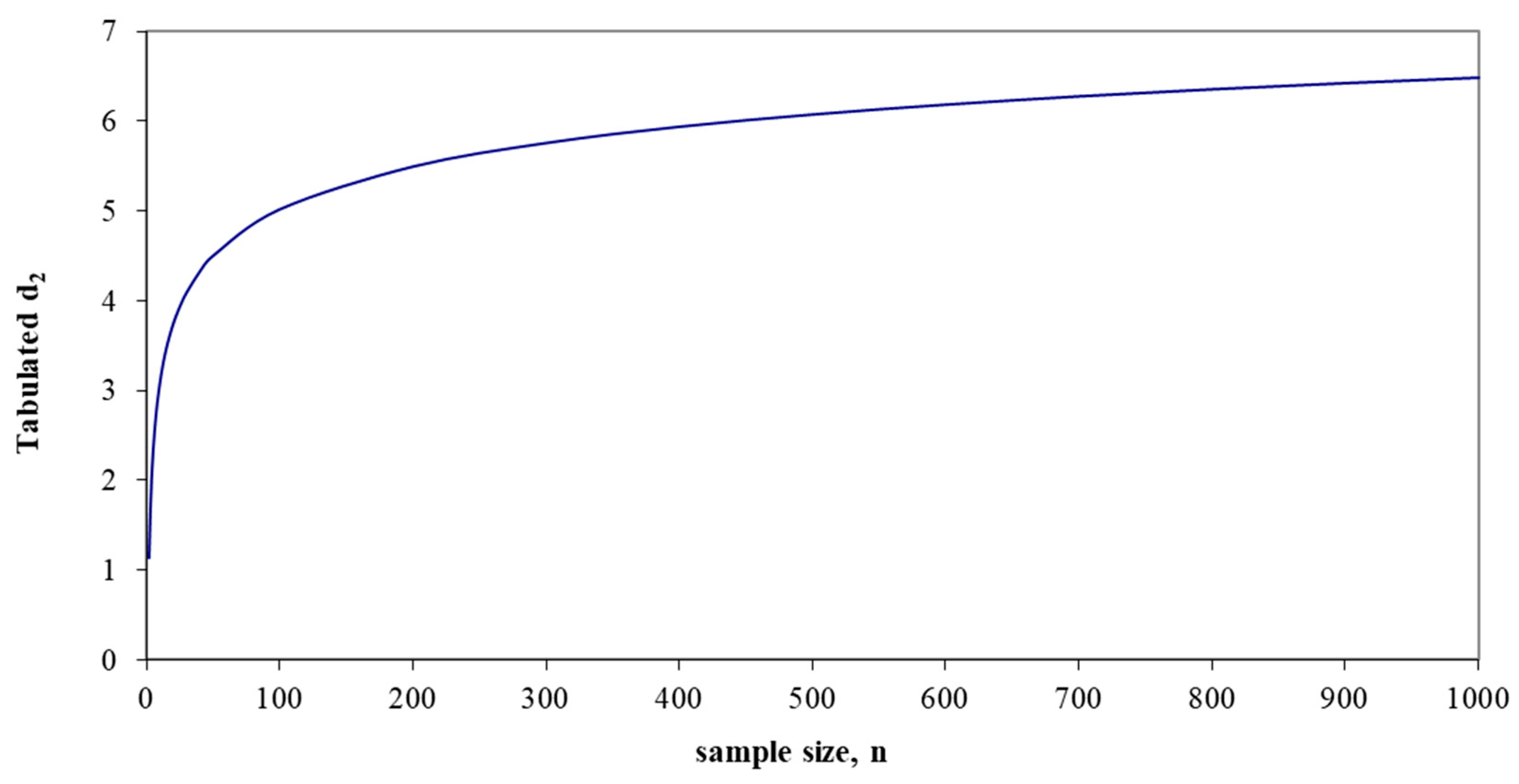
2.1. Approximations to d2 and d3 for Samples Sizes of at Least 6

As mentioned above, we are not familiar with analytical solutions to expressions (1)–(3) when the sample size exceeds 5. However, numerical values of the control chart constants d2 and d3 are widely available. In this section, we describe how the numerical values were used to develop rational function approximations. Other authors have developed approximations for the moments of order statistics of normal random variables (see [11,12] for summaries of some of these methods; see [13] as well). We believe that these earlier approximations have at least three limitations. First, some approximations are less accurate, especially for extreme order statistics (those used to compute the range). Second, the methods are more complicated than those presented in this study. Third, some methods require the use of tabulated moments of neighboring order statistics, which defeats the purpose of having approximations that do not require table lookup procedures.

Approximation Method

We focus on the method for approximating d2. The method was essentially the same for finding d3. We began by plotting the tabulated values of d2 as a function of the sample size n for values ranging from 2 to 1000, as given in [14] (We also used the values from [15] for d3. We note that the tabulated values of [14] were presented to 5 decimal places and those of [15] were to 15 places). Figure 1 shows a plot that suggests that d2 is a function of the logarithm of n. Hence, we sought an approximation relating the control chart constant values to the logarithm of n.
While numerous methods exist for estimating discrete values, we determined that a rational-function approximation would work well for this application. First, rational functions include polynomials (when the order of the polynomial in the denominator is of order 0). Second, other options such as splines, can result in more complex functions, and we wanted relatively simple expressions. Third, the rational functions have desirable asymptotic characteristics. For these and other advantages, see [16].
Instead of using a global measure of approximation error, such as the mean square error (MSE), we used the minimization of the maximum error between the approximations and the tabulated values of the control chart constants as our objective (As a final reason for using rational-function approximations rather than splines, we did look briefly at spline estimates and found that our rational function approximations resulted in smaller maximum errors). While MSE or mean absolute error (MAE) may be more appropriate if the overall accuracy of the approximation is important, we desired to ensure that the estimate of the control chart constants at every value of n was as close as possible to the tabulated values. Using MSE or MAE may result in an aggregate lower error, but it may do so at the expense of a few estimates having larger errors than desired. In other words, minimizing the maximum error is useful for guaranteeing worst-case (lack of) accuracy.
Because d2 is defined on a discrete point set rather than on an interval, we used the differential correction method to determine the Chebyshev minimax approximations [17]. The algorithm is an iterative one that seeks to minimize the maximum difference between the rational function, Rmk(n) and the tabulated values of d2, where
R m k n = j = 0 m a j log n j j = 0 k b j log n j ,   with   b 0 = 1 .
In (4), m is the order of the polynomial in the numerator of the rational function, k is the order of the denominator, and aj and bj are the coefficients of the numerator and denominator polynomials.
An initial rational function estimate is required to begin the procedure. We used multiple (polynomial) regression to find an initial polynomial solution and then used the minimax algorithm to convert the polynomial expression into a rational expression. The regression solutions were quite accurate, but in all cases, the estimates were improved by using the differential correction method.
The two parameters, m and k, can be adjusted to obtain better approximations. Generally, increasing m + k improves the accuracy of the estimates. Hence, we tried different combinations of parameters to find accurate and parsimonious approximations. For d2, we tried m + k values from 2 to 9, and for d3, we used values from 4 to 10. Combinations with sums greater than 9 (or 10 for d3) did not yield significant improvements in accuracy and were discarded in the interest of parsimony. Combinations with sums less than 2 (4 for d3) yielded unacceptable maximum errors.
We note that not all tabulated values were used for the computations. For d2 we used tabulated values for n = 2 (1) 25, 30 (10) 50, 100 (100) 1000. For d3, we used tabulated values for n = 2 (1) 25, 30 (5) 60, 70 (10) 100, 200, 500, and 1000 (the last three tabulated values were taken from [14] and were presented to only three decimal places). Removing some of the intermediate values where the curve in Figure 1 is relatively flat results in a more manageable optimization problem. As a post-hoc check, we evaluated the preferred rational function expressions at sample sizes 2 (1) 500 and 510 (10) 1000 for d2 and 2 (1) 100 for d3 and found only a few cases where the error only slightly exceeded the maximum error calculated during the estimation procedure (See Table 4 in the Results section for the preferred functions and the associated errors).

3. Results

We begin by presenting the analytical results for the first two moments of the range distribution for sample sizes 2 through 5. We then provide the results for the rational function approximations for larger sample sizes.

3.1. Analytical Results for n = 2, 3, 4 and 5

When n = 2, (1) simplifies substantially, and the solutions to (1)–(3) are straightforward. When n = 3, 4, and 5, the analytical solutions are not as simple. Ref. [18] showed that the pdf for the range when the sample size is 3 can be expressed as
f R r = 6 π 2 exp r 2 4 0 r / 6 exp u 2 2 d u = 6 π exp r 2 4 Φ r 6 1 2 .
They also showed that the ith moment μi of the distribution about the origin is
μ i = 3 π 2 i + 1 Γ i 2 + 1 0 π / 6 cos i θ d θ .
Other researchers have found moments of order statistics for samples of sizes 4 and 5. For a listing of these researchers and a description of the derivation by [19], see [20]. The author’s alternative derivations are provided in Appendix A. Table 1 summarizes the analytical results.
The analytical results reveal some common elements. For example, the arc tangent function and the term π3/2 appear in most of the d2 results. Despite these commonalities, we were unable to induce expressions for general sample sizes. Instead, in the next sections, we present accurate rational function approximations.

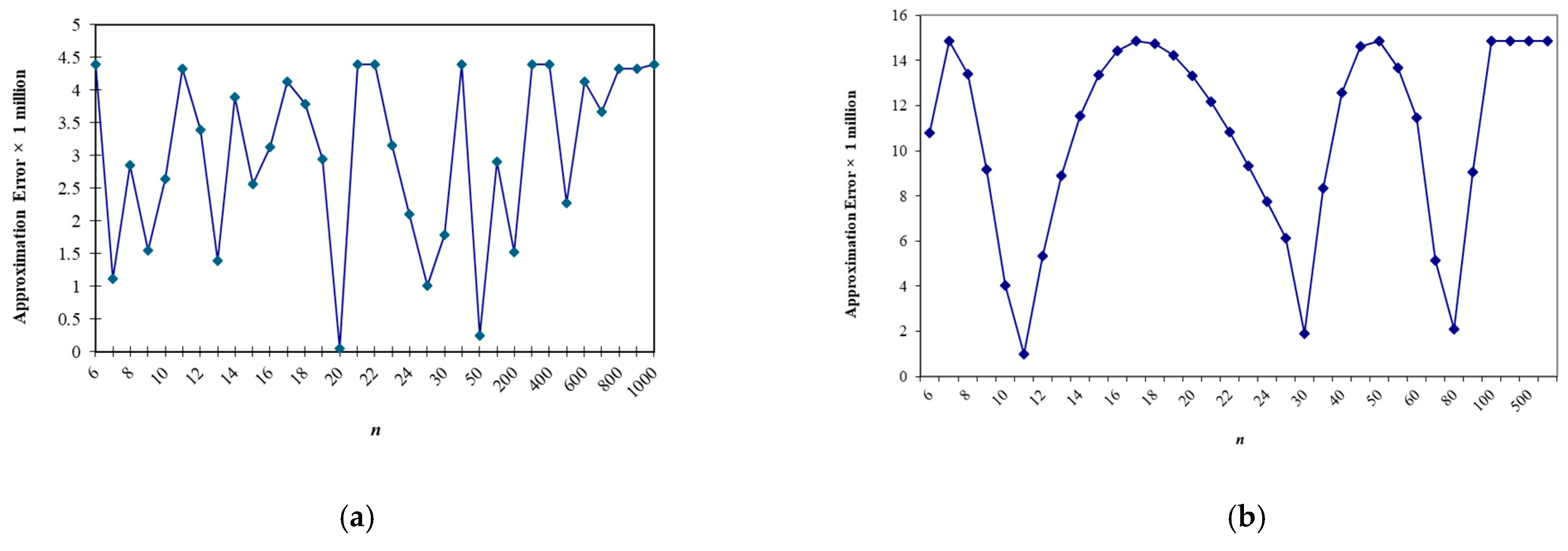
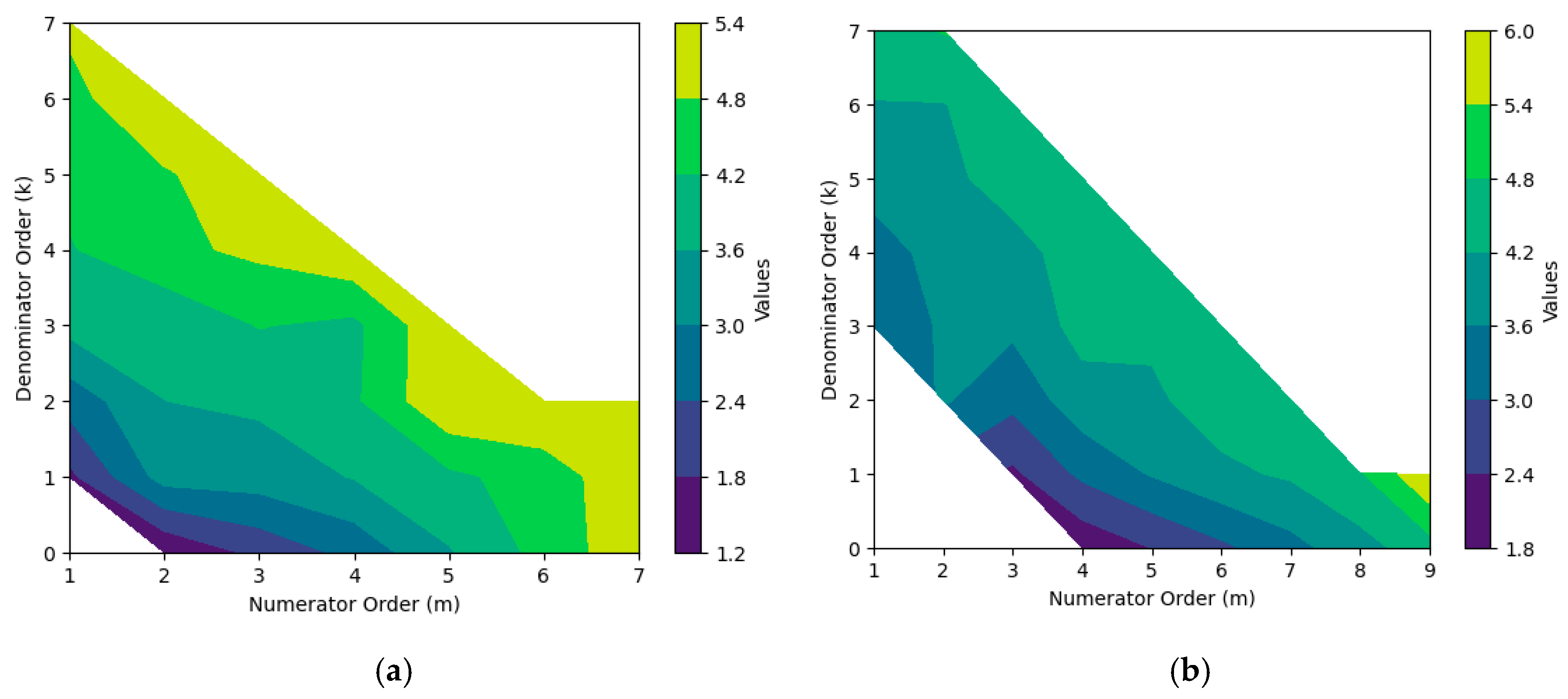
3.2. Approximation Results

Table 2 summarizes the results for the d2 approximations, and Table 3 summarizes the results for the d3 approximations. The tables show the values of m and k, the maximum error for the given rational function, and the coefficient values defined in (4). The tables are sorted first by the number of parameters (i.e., by m + k) and then by the maximum error. For the sake of brevity, the tables only show the case for a given m + k for which the maximum error is the smallest (More complete tables are given in Appendix B). For example, the first entry in Table 2 is for a rational function with m = 7 and k = 2. The maximum error for such a case was 4.3685 × 10⁻⁶, and the rational function approximation was
R 72 x = 4.683 × 10 5 + 4.1602 x 1.0722 x 2 + 0.2863 x 3 0.0791 x 4 + 0.0129 x 5 0.0012 x 6 + 4.363 × 10 5 x 7 1 + 0.1108 x 0.0363 x 2 ,
where x = log(n).

4. Discussion

Table 2 shows that the smallest maximum error was reported for the m + k = 9 case. We have only reported this case to show that a few of the m + k = 8 cases were very comparable in terms of their maximum error. The table also shows that there was no one systematically preferred form of the rational function approximations. For example, when m + k = 8, the best rational function approximation had more terms in the denominator (m = 2 and k = 6) than in the numerator; however, when m + k = 7, the lowest error was obtained from a rational function with more terms in the numerator (m = 5 and k = 2). Finally, the table shows that the d2 terms can be accurately estimated to at least three decimal places (maximum errors on the order of 10−4) with rational functions having as few as five total terms (m + k = 4). The approximations are very good with only eight total terms, having maximum errors on the order of 10−6. Such accuracy is remarkable given that the tabulated values used for the estimation were only given to five decimal places. Hence, very accurate estimates of d2 can be made for sample sizes from 2 to 1000 using simple algebraic expressions.
Similar results were obtained for d3, although the approximations were not as good. To achieve maximum errors on the order of 10−6, m + k must be as high as 10. With a total of eight terms (m + k = 7), some maximum errors were just over 10−5, which is still very good. We believe that greater accuracy is worth sacrificing a small degree of parsimony in the expression. We suggest using the rational functions shown in the second rows of Table 2 and Table 3, as they provide excellent accuracy with reasonably sized rational functions. Table 4 summarizes our suggestions for determining when finding the values of d2 and d3 for sample sizes of 2 to 1000. Moreover, Figure 2 shows plots of the difference between the actual and estimated values of the control chart constants for the suggested expressions for sample sizes greater than 5. As can be seen in the figure, the error oscillates, and in some cases, it is much smaller than the maximum error.
While we recommend the expressions in Table 4, others may prefer a different combination of parsimony and accuracy. Appendix B shows more complete tables of the estimated expressions and their maximum errors, which can be used to determine the preferred combination. Similarly, Figure 3 shows the contour plots of the negative logarithm of the maximum error for different combinations of the orders of the polynomials in the rational functions. Higher values in the plot indicate lower errors. For example, a value of 5 in the plot is associated with a maximum error of 1 × 10⁻⁵.

5. Conclusions

We have provided algebraic expressions that can be used to easily compute the control chart constants d2 and d3 for sample sizes from 2 to 1000. For the cases of n = 2 through 5 we have reviewed the exact solutions, whereas for cases of n > 5, we have provided rational function approximations that are very accurate. Other constants that are based on range control charts (e.g., A2, D3, and D4) can easily be computed from the two constants d2 and d3 (see [21] for example). Such expressions allow control chart designers and users, including control chart software producers, to compute the control chart constants without using lookup routines, which generally find control chart constants for a limited number of possible sample sizes with limited precision. Hence, the expressions simplify the process of automating the range control chart construction.

Funding

This research received no external funding.

Data Availability Statement

The data used for this project consisted only of the tabulated control chart constants given in [14,15] as described in Section 2.1.

Conflicts of Interest

The author declare no conflict of interest.

Appendix A

Author’s derivation of the analytical solutions for the first two moments of the range for sample sizes of four and five.

Appendix A.1. Derivation of the Expected Value of the Range for n = 4 and 5

We first note that from the definition of the standard normal pdf, we can rewrite the latter part of the integrand of (1) as
ϕ t + r 2 ϕ t r 2 = 1 2 π exp ( t 2 ) exp r 2 4 .
For ease of exposition, we can use (A1) we can rewrite (1) as
f R r = n n 1 exp r 2 4 2 π I n r ,
where
I n r = Φ t + r 2 Φ t r 2 n 2 exp t 2 d t .
From the definition of expected value we have
E R = n n 1 2 π 0 r exp r 2 4 I n r d r .
We can integrate (A4) by parts to obtain
E R = n n 1 π 0 exp r 2 4 d I n r d r d r
where
d I n r d r = n 2 2 2 π exp r 2 12 J n r
and
J n r = Φ t + r 2 Φ t r 2 n 3 exp 1 2 3 t + r 12 2 + exp 1 2 3 t r 12 2 d t
Substituting z = 3 t + r 12 in the first exponent and z = 3 t r 12 in the second, (A7) becomes
J n r = 1 3 e z 2 2 Φ z 3 + r 3 Φ z 3 2 r 3 n 3 + Φ z 3 + 2 r 3 Φ z 3 r 3 n 3 d z
We can evaluate (A8) by taking the derivative of Jn with respect to r, evaluating the resulting integral with respect to z, and then integrating again with respect to r. The result is that
d J n r d r = n 3 3 3 e z 2 2 Φ z 3 + r 3 Φ z 3 2 r 3 n 4 ϕ z 3 + r 3 + 2 ϕ z 3 2 r 3 d z + e z 2 2 Φ z 3 + 2 r 3 Φ z 3 r 3 n 4 2 ϕ z 3 + 2 r 3 + ϕ z 3 r 3 d z .
Expression (A9) has several products of the form e z 2 2 ϕ z 3 + k r 3 , which can be recombined to obtain 1 2 π exp k 2 r 2 24 exp 1 2 2 z 3 + k r 6 2 . We can further substitute for z using u = 2 z 3 + k r 6 , which gives
d J n r d r = n 3 6 2 π e r 2 24 e u 2 2 Φ u 2 + r 4 Φ u 2 3 r 4 n 4 + Φ u 2 + 3 r 4 Φ u 2 r 4 n 4 d u + 4 e r 2 6 e u 2 2 Φ u 2 + r 2 Φ u 2 r 2 n 4 d u .
We now consider the special cases of n = 4 and n = 5.

Appendix A.1.1. n = 4 Case

In this case (A10) simplifies to
d J 4 r d r = 1 3 e r 2 24 + 2 e r 2 6
and so
J 4 r = 2 6 π 3 Φ r 12 + Φ r 3 1 .
Using (A12) in (A6) and then (A5) for n = 4 gives
E R = 8 3 π 0 exp r 2 3 Φ r 12 + Φ r 3 1 d r .
To find (A13) we evaluate the three terms separately, which we will call K1, K2 and K3 (so that E R = 8 3 π K 1 + K 2 K 3 ). The integral K3 is straightforward and is 3 π / 2 . The other two are of the same form K,
K = 0 exp r 2 3 Φ r b d r = 1 2 π 0 exp r 2 3 d r r / b exp u 2 2 d u
We will use the same technique as [18], which is to substitute v = u r into (A14) and change the order of integration. The result is
K = 1 2 π 1 / b 0 r exp ( v r ) 2 2 exp r 2 3 d r d v = 1 2 π 1 / b 0 r exp r 2 3 1 + v 2 2 / 3 d r d v .
We can now evaluate (A15) with respect to r, giving
K = 3 2 2 π 1 / b 1 + 3 v 2 2 1 d v
We now let v = 2 3 tan θ and obtain
K = 3 2 π π / 2 tan 1 3 2 b θ d θ = 3 2 π tan 1 3 2 b + π / 2 .
Comparing this result to the terms in (A13) shows that
K 1 = 3 2 π tan 1 1 8 + π / 2
and
K 2 = 3 2 π tan 1 1 2 + π / 2 .
Hence we have that
E R = 8 3 π 3 2 π tan 1 1 8 + tan 1 1 2 + π 3 π 2 ,
which simplifies to
E R = d 2 = 12 π π tan 1 2 .

Appendix A.1.2. n = 5 Case

If we substitute n = 5 into (A10) we obtain
d J 5 r d r = 1 3 2 π e r 2 24 e u 2 2 Φ u 2 + r 4 Φ u 2 3 r 4 + Φ u 2 + 3 r 4 Φ u 2 r 4 d u + 4 e r 2 6 e u 2 2 Φ u 2 + r 2 Φ u 2 r 2 d u .
We can evaluate the integrals in (A22) by differentiating with respect to r first, then integrating with respect to u, and finally integrating again with respect to r. The first integral then is 2 2 π Φ r 20 + Φ 3 r 20 1 and the second integral is 2 2 π Φ r 5 1 2 . Hence we have
d J 5 r d r = 2 3 e r 2 24 Φ r 20 + Φ 3 r 20 1 + 8 3 e r 2 6 Φ r 5 1 2 .
If we combine (A5) and (A6) for n = 5 we have
E R = 30 π 2 π 0 exp r 2 3 J 5 r d r .
We can integrate (A24) by parts again to obtain
E R = 60 π 30 3 π 2 0 Φ 2 3 r d J 5 r d r d r = 60 π 20 3 π 2 0 Φ 2 3 r e r 2 24 Φ r 20 + Φ 3 r 20 1 + 4 e r 2 6 Φ r 5 1 2 d r .
To evaluate E(R) now, we must be able to evaluate integrals of the form L = 0 e r 2 a Φ 2 3 r Φ r b d r . We will do so by integrating by parts, letting u = Φ 2 3 r and dv = e r 2 a Φ r b d r . We can easily find du, but finding v is much more difficult. I will again use the method of [18]. First write v as v = 1 2 π exp x 2 a x b exp z 2 2 d z d x . Now let y = z x in the second of these integrals, and then reverse the order of integration. The result is v = 1 2 π 1 b x exp x 2 a x 2 y 2 2 d x d y . We can now evaluate the inside integral to obtain
v = 1 2 2 π 1 b exp r 2 a r 2 y 2 2 1 a + y 2 2 d y = 1 2 2 π e r 2 a 1 b e r 2 y 2 2 1 a + y 2 2 d y .
Now we have that L = 0 u d v = u v 0 0 v d u =   1 4 2 π 2 a tan 1 a 2 b + π a 2 + 1 2 π 6 0 e r 2 a e r 2 3 1 b e r 2 y 2 2 1 a + y 2 2 d y d r or
L = 1 4 2 π 2 a tan 1 a 2 b + π a 2 + a π 6 0 1 b exp r 2 2 y 2 + 2 a + 2 3 2 + a y 2 d y d r .
For simplicity, let β = y 2 + 2 a + 2 3 and reverse the order of integration to get
L = 1 4 2 π 2 a tan 1 a 2 b + π a 2 + a π 6 1 b 1 2 + a y 2 0 exp β r 2 2 d r d y .
The inner definite integral can now be evaluated, so that we have
L = 1 4 2 π 2 a tan 1 a 2 b + π a 2 + a 2 a π 1 b d y 2 + a y 2 3 a y 2 + 2 a + 6 .
The last integral can now be evaluated and gives
L = 1 4 2 π 2 a tan 1 a 2 b + π a 2 + 1 4 a π sin 1 a 2 a + 2 b 6 + 2 a + sin 1 2 a 6 + 2 a
The other terms in (A25) have the form K = 0 e r 2 a Φ 2 3 r d r . From the n = 4 case we know that K = a 2 π tan 1 a 3 + π 2 . Now we can combine this result with (A30) and substitute them for the appropriate terms in (A25). After (a large amount of) simplification, the result is that E(R) = 30 π 3 / 2 tan 1 2 5 π .

Appendix A.2. Derivation of the Variance of the Range for n = 4 and 5

We again begin with the case for general n and use (A2) and (A3) as a base. To find the variance of the range, we first find E(R2),
E R 2 = n n 1 2 π 0 r 2 exp r 2 4 I n r d r .
First, we can integrate this by parts to obtain
E R 2 = n n 1 π 0 r exp r 2 4 d I n r d r d r + 0 exp r 2 4 I n r d r
where d I n r d r is defined in (A6). By noting that the integrand of the second term in (A32) is essentially fR(r), and by using (A6) and (A7) we can simplify (A32) to
E R 2 = 2 + n n 1 n 2 2 π 3 / 2 0 r exp r 2 3 J n r d r .
where Jn(r) is defined in (A8). Integrating by parts once again gives
E R 2 = 2 + 3 n n 1 n 2 2 2 π 3 / 2 0 exp r 2 3 d J n r d r d r
where d J n r d r is defined in (A12).
For the n = 4 case we can substitute (A11) into (A34) and integrate to find that E(R2) is 2 π + 2 3 + 6 π .
For the case of n = 5, we can use (A23) in (A34) to obtain
E R 2 = 2 + 60 2 π 3 / 2 0 e 3 r 2 8 Φ r 20 + Φ 3 r 20 1 + 4 e r 2 2 Φ r 5 1 2 d r
We have already seen in Appendix A.1 that integrals like most of those found in (A35) can be found using (A14)–(A17). Hence (A35) simplifies to E(R2) = 2 π 2 + 10 3 tan 1 5 3 + 2 3 tan 1 1 5 π 2 .

Appendix B. Complete Tables for the Rational Function Approximations

Table A1. Rational function values for approximating the control chart constant d2 (see (4) for definitions of the terms used in the table). Due to the large number of parameters, the table is divided based on the values of m + k. In the first column, “a” refers to the coefficients in the numerator of the rational function approximation, while “b” refers to the coefficients in the denominator (See expression (4) in Section 2).
a. m + k = 9.
(m, k)(7, 2)
Maximum Error4.37 × 10−6
a0−4.68 × 10⁻⁵
a14.1601706
a2−1.072159
a30.2862847
a4−0.0791025
a50.0128782
a6−0.0011768
a74.36 × 10−5
b10.1108409
b2−0.036305
b. m + k = 8.
(m, k)(2, 6)(8, 0)(6, 2)(5, 3)(4, 4)(7, 1)(3, 5)(1, 7)
Maximum Error4.39 × 10−64.40 × 10−64.45 × 10−64.50 × 10−64.82 × 10−65.69 × 10−66.68 × 10−61.23 × 10⁻⁵
a00.00021170.0001602−0.00039990.00038580.00054540.00039890.0017505−0.0022132
a14.1577144.15822594.16278984.15616164.15456754.15615464.14245084.1789954
a20.3491476−1.5259333−0.9500651.45379050.7921954−1.51177884.4979643
a3 0.59246880.20927840.2428315−0.27923720.5775411−1.3731118
a4 −0.1840047−0.0564231−0.0142767−0.1098239−0.1706958
a5 0.04297720.00769550.0007023 0.0354162
a6 −0.0070858−0.000464 −0.0045255
a7 0.0007349 0.0002648
a8 −3.60 × 10⁻⁵
b10.4502653 0.14202910.714540.55392260.00171241.43322450.3843422
b20.0245085 −0.04620270.18238150.0012477 0.0864897−0.0338921
b3−0.0137816 0.0005872−0.0705542 −0.17168550.0137563
b40.004125 −0.0034663 0.0147776−0.0105444
b5−0.0006383 −0.00080950.0043436
b64.18 × 10−5 −0.0008831
b7 7.16 × 10⁻⁵
c. m + k = 7.
(m, k)(5, 2)(7, 0)(3, 4)(2, 5)(1, 6)(6, 1)(4, 3)
Maximum Error4.52 × 10−65.76 × 10−61.20 × 10−51.83 × 10−52.47 × 10−53.36 × 10−58.85 × 10−5
a00.00039450.0004069−0.00134290.0674587−0.00231360.0019498−0.0049402
a14.15608084.15608774.17067313.55331934.17790374.1446034.1994308
a21.4690251−1.5186854−0.6775001133.74141 −1.4869875−3.479488
a30.23910450.57980190.3559161 0.53532910.697147
a4−0.0147213−0.1713809 −0.1377470.0833977
a50.00070210.0355484 0.0215142
a6 −0.0045384 −0.0015042
a7 0.0002651
b10.7181305 0.213783132.0018510.3814535−0.0001152−0.4379041
b20.1829496 0.004663612.604867−0.0254915 −0.1903784
b3 0.0331532−1.02690530.0018241 0.1142485
b4 −0.00131960.0535564−0.0014589
b5 0.00108650.0005456
b6 −6.26 × 10⁻⁵
d. m + k = 6.
(m, k)(2, 4)(6, 0)(1, 5)(3, 3)(4, 2)(5, 1)
Maximum Error2.18 × 10−54.01 × 10−54.13 × 10−55.93 × 10−57.91 × 10−58.66 × 10⁻⁵
a00.07408630.0021644−0.00248410.1112902−0.0039991−0.004793
a13.50035524.14318184.17796433.23009014.18882884.1941431
a2133.77185−1.4831307 112.82908−0.52613950.4951024
a3 0.5314118 13.842787−0.0412288−0.0515586
a4 −0.1356001 −0.00238280.0141002
a5 0.0209355 −0.0016136
a6 −0.0014438
b131.970664 0.380388126.7699610.26106450.5094877
b212.65184 −0.022300314.24345−0.0863658
b3−1.0557861 −0.00196630.2333121
b40.0625968 0.0007101
b5 −4.89 × 10⁻⁵
e. m + k = 5.
(m, k)(1, 4)(2, 3)(3, 2)(4, 1)(5, 0)
Maximum Error7.04 × 10−51.93 × 10−41.98 × 10−42.34 × 10−42.81 × 10−4
a0−0.0021528−0.0068195−0.0069689−0.00795740.0087059
a14.17780964.20485594.20564634.21180954.1014476
a2 0.33898550.42314830.4123636−1.3881892
a3 0.0040529−0.00938440.4305764
a4 0.0008702−0.0815235
a5 0.0067557
b10.38128610.47609230.4966020.4973312
b2−0.0240701−0.00190420.0066181
b3−0.00066610.0001546
b40.0002934
f. m + k = 4.
(m, k)(1, 3)(2, 2)(3, 1)(4, 0)
Maximum Error1.61 × 10−42.53 × 10−45.07 × 10−42.61 × 10⁻³
a0−0.0058338−0.0046286−0.01232970.0390467
a14.19907414.19623774.23433233.9449081
a2 0.34171140.4466871−1.1263646
a3 −0.00820.2442248
a4 −0.0227788
b10.39193650.47384050.5145802
b2−0.0310113−0.0006776
b30.0016884
g. m + k = 3 and m + k = 2.
m + k33322
(m, k)(2, 1)(1, 2)(3, 0)(1, 1)(2, 0)
Maximum Error5.61 × 10−42.35 × 10−31.09 × 10−22.19 × 10−25.80 × 10−2
a0−0.00232130.01721510.10086290.12951860.2907984
a14.18711424.09377563.68224713.66813333.0786409
a20.3449063 −0.8018105 −0.3446446
a3 0.0949052
b10.47209720.3546785 0.2410842
b2 −0.0184772
Table A2. Rational function values for approximating the control chart constant d3 (see (4) for definitions of the terms used in the table). Due to the large number of parameters, the table is divided based on the values of m + k. In the first column, “a” refers to the coefficients in the numerator of the rational function approximation, while “b” refers to the coefficients in the denominator. (See expression (4) in Section 2).
a. m + k = 10.
(m, k)(9, 1)
Maximum Error1.04 × 10−6
a00.315104
a15.547612
a2−2.84442
a3−0.78335
a42.852878
a5−2.51086
a61.234777
a7−0.36344
a80.059829
a9−0.00424
b13.396075
b. m + k = 9.
(m, k)(2, 7)(7, 2)(8, 1)(6, 3)(9, 0)(4, 5)(3, 6)(5, 4)
Maximum Error1.49 × 10−51.67 × 10−51.83 × 10−52.13 × 10−52.85 × 10−53.40 × 10−53.46 × 10−53.48 × 10⁻⁵
a00.2228740.2966840.2882690.2823650.425844−0.845970.4151480.416896
a17.4350755.725385.8248495.812922.891117156.15994.1403623.804773
a2−1.74755−2.7717−3.84618−5.82438−7.152651102.0122.558952−0.02747
a3 0.8020641.3695293.5232249.656155−308.826−1.32839−0.29831
a4 0.2000330.068175−1.19533−8.5306−24.3344 −0.03858
a5 −0.2218−0.268920.2300265.088273 −0.00149
a6 0.0631960.104807−0.01879−2.024
a7 −0.00636−0.0174 0.512864
a8 0.00106 −0.07467
a9 0.004743
b15.4373823.4601183.4214733.145292 330.48892.796542.043444
b20.1384150.668103 −0.99902 514.49133.5346852.385689
b32.584673 0.379228 605.69430.912601−0.35895
b4−2.56493 −303.519−1.08252−0.23241
b51.00801 11.366190.102501
b6−0.20567 −0.0042
b70.017412
c. m + k = 8.
(m, k)(1, 7)(6, 2)(4, 4)(3, 5)(5, 3)(7, 1)(2, 6)(8, 0)
Maximum Error2.63 × 10−53.29 × 10−53.49 × 10−53.65 × 10−54.85 × 10−55.25 × 10−56.56 × 10−51.06 × 10⁻⁴
a0−0.222020.3612970.4174480.4198770.4378440.196180.4648820.457687
a116.8094.6048743.7130193.5982933.3911737.403562.9364552.580339
a2 −3.34365−0.73609−1.34281−0.28428−3.571520.112444−5.92177
a3 2.01313−0.123180.036971−0.28680.096022 7.037428
a4 −0.72414−0.0197 0.0434831.070521 −5.20663
a5 0.145333 −0.00508−0.62695 2.458343
a6 −0.01238 0.153482 −0.71801
a7 −0.01431 0.117911
a8 −0.00831
b115.375982.360911.8393651.6293581.602544.9052371.221915
b2−2.998820.4588872.047781.7687782.332491 2.699692
b314.3693 −0.74976−1.10774−0.79915 −0.76911
b4−10.1252 −0.057820.117442 0.336715
b53.946838 −0.00475 −0.09027
b6−0.83038 0.009819
b70.072844
d. m + k = 7.
(m, k)(4, 3)(1, 6)(5, 2)(6, 1)(2, 5)(3, 4)(7, 0)
Maximum Error3.90 × 10−56.68 × 10−57.97 × 10−58.37 × 10−58.73 × 10−59.96 × 10−54.00 × 10−4
a00.4145790.4483640.5146990.2674890.3546280.3472220.506673
a13.7181223.1717762.3575095.9985344.6678524.7010322.154437
a2−0.92875 3.387868−4.38089−0.57936−1.3774−4.46778
a3−0.07681 −1.250342.220661 0.2840864.464941
a4−0.00913 0.32038−0.68974 −2.59734
a5 −0.0330.120869 0.887721
a6 −0.00918 −0.1648
a7 0.012798
b11.8024981.4074581.176193.4256012.6754022.570444
b21.9760012.6523344.470245 2.2858311.913318
b3−0.86642−0.74001 −0.33457−0.66506
b4 0.292182 −0.065110.143048
b5 −0.07846 0.012773
b6 0.008683
e. m + k = 6.
(m, k)(4, 2)(1, 5)(2, 4)(3, 3)(5, 1)(6, 0)
Maximum Error1.10 × 10−41.28 × 10−41.36 × 10−41.91 × 10−42.26 × 10−41.34 × 10⁻³
a00.3427480.4278340.4443210.4752740.2172240.569274
a14.9647473.7196383.3780072.9958766.9159921.677416
a2−0.67509 −0.515290.213881−4.33346−3.09547
a30.305956 −0.054691.7497742.508293
a4−0.03384 −0.37293−1.08081
a5 0.0324280.239276
a6 −0.02135
b12.9735672.0117611.6132631.415014.279257
b22.1791082.3535282.0874422.394381
b3 −0.12915−0.59247−0.25408
b4 −0.040590.040986
b5 0.007675
f. m + k = 5.
(m, k)(2, 3)(1, 4)(3, 2)(4, 1)(5, 0)
Maximum Error2.03 × 10−45.27 × 10−46.82 × 10−47.5 × 10−43.88 × 10−4
a00.4573810.5230990.576235−0.058480.650202
a13.2327912.3957381.70951211.175651.145273
a20.559042 0.826375−5.5501−1.84151
a3 −0.055611.5949771.130005
a4 −0.17954−0.31863
a5 0.034104
b11.6486050.9401910.511297.753653
b22.658812.0425142.324483
b30.024817−0.35739
b4 0.036746
g. m + k = 4.
(m, k)(2, 2)(1, 3)(3, 1)(4, 0)
Maximum Error2.13 × 10−48.98 × 10−45.25 × 10−31.08 × 10⁻²
a00.4528620.476886−1.420470.762477
a13.3389773.23019636.396870.533722
a20.491674 −12.4903−0.74534
a3 1.8323430.295284
a4 −0.03852
b11.7373531.69432429.41969
b22.638292.130666
b3 −0.17919

References

  1. Snee, R.D. Statistical Thinking and Its Contribution to Total Quality. Am. Stat. 1990, 44, 116–121. [Google Scholar] [CrossRef]
  2. Hoerl, R.W.; Snee, R.D.; De Veaux, R.D. Applying Statistical Thinking to ‘Big Data’ Problems. WIREs Comput. Stat. 2014, 6, 222–232. [Google Scholar] [CrossRef]
  3. Hoerl, R.W.; Snee, R.D. Statistical Thinking: Improving Business Performance; Wiley: Hoboken, NJ, USA, 2020. [Google Scholar]
  4. Khoo, M.B.; Lim, E.G. An Improved R (Range) Control Chart for Monitoring the Process Variance. Qual. Reliab. Eng. Int. 2005, 21, 43–50. [Google Scholar] [CrossRef]
  5. Chen, W.H.; Tirupati, D. On-line Quality Management: Integration of Product Inspection and Process Control. Prod. Oper. Manag. 1995, 4, 242–262. [Google Scholar] [CrossRef]
  6. Wardell, D.G. Algebraic Expressions for Range Control Chart Constants. In Proceedings of the Fiftieth Annual Meeting of the Western Decision Sciences Institute, Waikoloa, HI, USA, 5–8 April 2022. [Google Scholar]
  7. Burr, I.W. The Effect of Non-normality on Constants for x ¯ and R charts. Ind. Qual. Control 1967, 23, 563–569. [Google Scholar]
  8. Qiu, P.; Zhang, J. On Phase II SPC in Cases When Normality is Invalid. Qual. Reliab. Eng. Int. 2015, 31, 27–35. [Google Scholar] [CrossRef]
  9. Khakifirooz, M.; Tercero-Gómeza, V.G.; Woodall, W.H. The Role of the Normal Distribution in Statistical Process Monitoring. Qual. Eng. 2021, 3, 497–510. [Google Scholar] [CrossRef]
  10. Mood, A.M.; Graybill, F.A.; Boes, D.C. Introduction to the Theory of Statistics; McGraw Hill: New York, NY, USA, 1974. [Google Scholar]
  11. David, H.A. Order Statistics; John Wiley & Sons, Inc.: New York, NY, USA, 1970. [Google Scholar]
  12. Arnold, B.C.; Balakrishnan, N. Relations, Bounds and Approximations for Order Statistic; Lecture Notes in Statistics No. 53; Springer: New York, NY, USA, 1989. [Google Scholar]
  13. Royston, J.P. Algorithm AS 177: Expected Normal Order Statistics (Exact and Approximate). Appl. Stat. 1982, 31, 161–165. [Google Scholar] [CrossRef]
  14. Pearson, E.S.; Hartley, H.O. (Eds.) Biometrika Tables for Statisticians; Biometrika Trust: London, UK, 1976; Volume 1. [Google Scholar]
  15. Harter, H.L.; Balakrishnan, N. Tables for the Use of Range and Studentized Range in Tests of Hypotheses; CRC Press: Boca Raton, FL, USA, 1998. [Google Scholar]
  16. Petrushev, P.P.; Popov, V.A. Rational Approximation of Real Functions; Cambridge University Press: Cambridge, UK, 2011. [Google Scholar]
  17. Ralston, A.; Rabinowitz, P. A First Course in Numerical Analysis; Dover Publications, Inc.: New York, NY, USA, 2001. [Google Scholar]
  18. McKay, A.T.; Pearson, E.S. A Note on the Distribution of Range in Samples of n. Biometrika 1933, 25, 415–420. [Google Scholar] [CrossRef]
  19. Bose, R.C.; Gupta, S.S. Moments of Order Statistics from a Normal Population. Biometrika 1959, 46, 433–440. [Google Scholar] [CrossRef]
  20. Balakrishnan, N.; Cohen, A.C. Order Statistics and Inference: Estimation Methods; Academic Press, Inc.: London, UK, 2014. [Google Scholar]
  21. Ryan, T.P. Statistical Methods for Quality Improvement; John Wiley and Sons: Weinheim, Germany, 2011. [Google Scholar]
Figure 1. Plot of the tabulated values of d2 as a function of sample size n. The plot suggests that the relationship between d2 and n is logarithmic.
Mathematics 13 01537 g001
Figure 2. Plots of the approximation errors for (a) d2 and (b) d3 for the rational functions listed in Table 4. The plots show the sample sizes for which the estimation error is the largest.
Mathematics 13 01537 g002
Figure 3. Contour plots of the negative logarithm of the maximum error for (a) d2 and (b) d3 for different combinations of the orders of the polynomials in (4). Larger values are associated with smaller errors.
Mathematics 13 01537 g003
Table 1. Analytical results for d2 and d3 for samples of sizes 2 through 5.
Sample Size nd2d3
2 2 / π 2 4 π
3 3 / π 2 π + 3 3 9 π
4 12 π π tan 1 2 2 π + 2 3 + 6 π d 2 2
5 30 π 3 / 2 tan 1 2 5 π 2 π 2 + 10 3 tan 1 5 3 + 2 3 tan 1 1 5 π 2 d 2 2
Table 2. Rational function values for approximating the control chart constant d2. These results are for the functions with the lowest errors for each combination of m + k. More complete tables are found in Appendix B. See (4) for definitions of the terms used in the table.
m + k98765432
(m, k)(7, 2)(2, 6)(5, 2)(2, 4)(1, 4)(1, 3)(2, 1)(1, 1)
Maximum Error4.3685 × 10−64.3907 × 10−64.5173 × 10−62.1767 × 10−57.0438 × 10−51.6052 × 10−45.6083 × 10−42.1880 × 10⁻²
a0−4.6830 × 10−50.000211680.000394460.0740863−0.0021528−0.0058338−0.00232130.12951861
a14.160170584.157713994.156080813.500355234.177809584.199074084.187114193.66813329
a2−1.0721590.349147571.4690251133.771848 0.34490634
a30.28628465 0.23910449
a4−0.0791025 −0.0147213
a50.01287818 0.00070213
a6−0.0011768
a74.36 × 10−5
b10.110840910.450265270.7181304631.9706640.381286120.39193650.472097160.24108419
b2−0.0363050.024508510.1829496312.6518404−0.0240701−0.0310113
b3 −0.0137816 −1.0557861−0.00066610.00168837
b4 0.00412501 0.062596790.00029336
b5 −0.0006383
b6 4.1793 × 10⁻⁵
Table 3. Rational function values for approximating the control chart constant d3. These results are for the functions with the lowest error for each combination of m + k. More complete tables are found in Appendix B. See (4) for definitions of the terms used in the table.
m + k10987654
(m, k)(9, 1)(2, 7)(1, 7)(4, 3)(4, 2)(2, 3)(2, 2)
Maximum Error1.0426 × 10−61.4861 × 10−52.6339 × 10−53.9049 × 10−51.1010 × 10−42.0261 × 10−42.1340 × 10−4
a00.3151040.222874−0.222020.4145790.3427480.4573810.452862
a15.5476127.43507516.8093.7181224.9647473.2327913.338977
a2−2.84442−1.74755 −0.92875−0.675090.5590420.491674
a3−0.78335 −0.076810.305956
a42.852878 −0.00913−0.03384
a5−2.51086
a61.234777
a7−0.36344
a80.059829
a9−0.00424
b13.3960755.43738215.375981.8024982.9735671.6486051.737353
b2 0.138415−2.998821.9760012.1791082.658812.63829
b3 2.58467314.3693−0.86642 0.024817
b4 −2.56493−10.1252
b5 1.008013.946838
b6 −0.20567−0.83038
b7 0.0174120.072844
Table 4. Suggested algebraic expressions for control chart constants d2 and d3 for sample sizes 2 to 1000. In the table, x = log(n).
a. Expressions for d2
Sample Size nExpression for d2Maximum Error
2 2 / π 0
3 3 / π 0
4 12 π π tan 1 2 0
5 30 π 3 / 2 tan 1 2 5 π 0
n = 6 to 1000 2.1168 × 10 4 + 4.1577 x + 0.3491 x 2 1 + 0.4503 x + 0.0245 x 2 0.0138 x 3 + 0.4125 × 10 3 x 4 6.383 × 10 4 x 5 + 4.1793 × 10 5 x 6 4.3907 × 10⁻⁶
b. Expressions for d3
Sample Size nExpression for d3Maximum Error
2 2 4 π 0
3 2 π + 3 3 9 π 0
4 2 π + 2 3 + 6 π d 2 2 0
5 2 π 2 + 10 3 tan 1 5 3 + 2 3 tan 1 1 5 π 2 d 2 2 0
n = 6 to 1000 0.2229 + 7.4351 x 1.7476 x 2   1 + 5.4374 x + 0.1384 x 2 + 2.5847 x 3 2.5649 x 4 + 1.0080 x 5 0.2057 x 6 + 0.0174 x 7   1.4861 × 10⁻⁵
Disclaimer/Publisher’s Note: The statements, opinions and data contained in all publications are solely those of the individual author(s) and contributor(s) and not of MDPI and/or the editor(s). MDPI and/or the editor(s) disclaim responsibility for any injury to people or property resulting from any ideas, methods, instructions or products referred to in the content.

