Article

On the Special Viviani’s Curve and Its Corresponding Smarandache Curves

1
School of Mathematics, Hangzhou Normal University, Hangzhou 311121, China
2
Department of Mathematics, Ordu University, Ordu 52200, Türkiye
*
Author to whom correspondence should be addressed.
Mathematics 2025, 13(9), 1526; https://doi.org/10.3390/math13091526
Submission received: 27 January 2025 / Revised: 27 April 2025 / Accepted: 2 May 2025 / Published: 6 May 2025
(This article belongs to the Special Issue Submanifolds in Metric Manifolds, 2nd Edition)

Abstract

:
In the present paper, the special Viviani’s curve is revisited in the context of Smarandache geometry. Accordingly, the paper first defines the special Smarandache curves of Viviani’s curve, including the Darboux vector. Then, it expresses the resulting Frenet apparatus for each Smarandache curve in terms of the Viviani’s curve. The paper is also supported by extensive graphical representations of Viviani’s curve and its Smarandache curves, as well as their respective curvatures.

1. Introduction and Preliminaries

The theory of curves has always been a popular subject in the context of differential geometry, which consequently led to the rise of some special curves in the field. A curve can be considered to be special in many ways. It may be a model for a particle motion or a representative image of an object which we encounter in daily life. For example, the orbits of planets can be represented by ellipses, and a parabola is used to model the trajectory of a projectile or referred in optics by its reflective property. These two curves with hyperbolas are also covered in many textbooks as a core chapter, namely conic sections. Moreover, a catenary curve (also known as a chain curve) can be used to form a suspension bridge [1,2]. Euler’s famous spiral curve is used as a transition curve in rail(-high)way engineering and has many applications to solve diffraction. Note that the curve has various names in the literature for some distinct scientific reasoning such as the partial of Bernoulli elastica curve, Fresnel’s spiral, Cornu’s spiral, the Glover spiral, the clothoid, etc. For more information, see [3]. The derivation of the curve is also based on the fundamental theory of plane curves [4,5,6].
The helices of space curves can be the representative image of DNA sequences. The general helices have another characteristic described by Lancret’s Theorem such that the ratio of curvature to torsion is constant [7]. This way of characterization can be followed by Bertrand’s curve [8], whose curvatures have a linear relation such that a κ + b τ = 1 for some a 0 , b R constants. A Mannheim curve [9], on the other hand, satisfies the relation κ = λ ( κ 2 + τ 2 ) for a constant λ R { 0 } . The Bertrand and Mannheim curves have other useful distinct properties for generating curve pairs by means of a Frenet frame. Associating curves one to another with some mathematical relations with respect to Frenet vectors is another important topic for the theory of curves. The involute and evolute curves can be considered as paired curves that are orthonormal tangential as well. They are very important curves for gear designs in mechanical engineering. Another curve with a curvature-themed characteristic is the Salkowski curve [10]. The curve is characterized by constant curvature and non-constant torsion. An anti-Salkowski curve, which naturally has a constant torsion and a non-constant curvature, is defined by taking the integrand of the binormal vector of the Salkowski curve [11]. Defining a curve pair by its integrands has been studied from different aspects and, most interestingly, with distinct names like binormal direction curves or adjoint or conjugate curves in [12,13,14].
Apart from these, the Viviani’s curve is another kind of special curve in many aspects. To the best of our knowledge, the curve was derived as a solution to Galileo’s proposed problem in the 17th century as how to build on a hemispherical cupola four equal windows of such a size that the remaining surface can be exactly squared [15]. As a solution to this problem, the Italian mathematician Vincenzo Viviani, who also assisted Galileo’s work at that time, introduced a curve by the intersection of a sphere with a cylinder which is tangent to the sphere and passing through the two poles of it. Some various projections of the curve onto some specific planes derived other special planar curves such as parabolas, circles, lemninscates, bifoliums, fish curves, Gutschoven’s kappa curves, etc. [16]. Although, the first introduced way of generating the Viviani’s curve depends on the intersection of a sphere and cylinder, there are other ways of defining it by intersecting a sphere with other types of familiar surfaces such as cones, parabolic cylinders, Mobius strips, etc. [15,16]. The curve was later recognized as the one special case of spherical Clelia’s curves which is characterized by the linear dependency of its coordinates under the parametrization of a spherical coordinate system [17]. In addition, the characteristics of the curve were first considered using Lorentz–Minkowski spaces in [18]. An interesting foundation for the relationship of the curve with quantum theory was given in [19]. Recent studies have expanded the understanding of special curves and surfaces and their singularities in different spaces [20,21,22], as well as the geometry of sweeping surfaces [23,24,25]. Furthermore, the exploration of Riemannian invariants and the convergence of quantization methods offer further insights into the geometric properties of submanifolds and their potential discretizations [26,27]. These results not only inspire our current work but also suggest new directions for future research, where the interactions between special curves and evolving geometric structures may yield novel applications in both classical geometry [28,29,30] and mathematical physics [31,32,33].
As previously mentioned, the derivation of new curves that are associated with a given specific curve is a subject of particular interest in the field. One method for deriving new curves from an existing one is to refer to Smarandache geometry. Smarandache geometry, as defined by Florentin Smarandache in 1969, is a type of geometry that relies on denying certain geometrical axioms. In doing so, it is claimed that the “axiom” is rendered false in at least two distinct ways, or, alternatively, that it is false and also sometimes true in the same geometric space. This process is referred to as Smarandachely denying the axiom. Regarding Euclid’s parallel postulate, Lobachevsky–Bolyai–Gauss (hyperbolic) and Riemannian (elliptic) geometries are some sub-special Smarandache geometries. These can also be unified in the same geometric space including the Euclidean (parabolic) geometry. It is also Florentin Smarandache who first argued his concept of multi-structures or multi-spaces in [34]. In reality, there are no isolated homogeneous spaces, but rather a mixture of interconnected spaces, each with a different structure. This is why Smarandache geometries (or sometimes hybrid geometries) are becoming increasingly popular. Further, Linfan Mao (2006), in his book, also calls a Smarandache multi-space a union of n different spaces equipped with some different structures, which can be used for both discrete and connected spaces, particularly for geometries and spacetimes in theoretical physics. He constructed a completed multi-space by exploiting the combinatorial design [35]. This combinatorial design was exploited by Turgut and Yılmaz in 2008, and, as a curve of a hybrid geometrical structure, they first defined a Smarandache curve whose position vector is a linear combination of a moving frame on and along the curve for Minkowski space in [36]. In a similar way, Ali (2010) [37] defined these curves in Euclidean three-space by utilizing Frenet frames. The curves are discussed in many studies using different frames and considering distinct spaces as well [38,39,40,41,42,43,44,45,46,47,48,49,50]. For those interested in pursuing further insights into Smarandache geometry and seeking further research opportunities, we kindly refer you to the comprehensive research repository, accessible at [51].
The motivation for the current paper is to reveal some other characteristics of the special Viviani’s curve through its Smarandache curves. Thus, the outline of the paper is as follows: First, a relatively comprehensive literature review along with the basic concepts such as the definition of Viviani’s curve and its Frenet apparatus are given in Section 1. Section 2 comprises information about Smarandache curves and their derivations. Frenet vectors and the curvatures of each Smarandache curve are expressed in terms of the invariants of Viviani’s curve. Both the two curvatures of Viviani’s curve and each Smarandache curve are the main interest for the paper. Therefore, each curve’s curvatures is examined following their graphical illustrations. Finally, in Section 3, we provide some concluding remarks and discuss the results.
Let α : I R E 3 be any curve of class at least C 2 in three-dimensional Euclidean space. Then, the Frenet trihedron denoted by { T , N , B } , the curvatures { κ , τ } , and their corresponding relations are given as
T = α α , N = B × T , B = α × α α × α ,
κ = α × α α 3 , τ = α × α , α α × α 2 ,
T = κ v N , N = κ v T + τ v B , B = τ v N .
Here, v = α , κ is the curvature, and τ is the torsion of α [2,38]. It is known that the Frenet vectors rotate instantaneously along the curve and this instantaneous rotation occurs around an axis spanned by a vector. This vector is called a Darboux vector, and, according to its definition, it has the following form:
W = τ T + κ B .
If w is considered to be the angle between the vectors B and W w = ( B , W ) , then we can write
κ = W cos w , τ = W sin w ,
and correspondingly derive the unit Darboux vector as
C = sin w T + cos w B ,
where cos w = κ κ 2 + τ 2 , sin w = τ κ 2 + τ 2 , and w = τ κ 1 + τ 2 κ 2 .
Moreover, as an intersection of the cylinder centered at point ( a , 0 , 0 ) with radius r = a and the sphere centered at origin ( 0 , 0 , 0 ) with radius r = 2 a , the special Viviani’s curve is defined as follows:
r ( t ) = a ( 1 + cos ( t ) ) , a sin ( t ) , 2 a sin t 2 , t [ 2 π , 2 π ] .
However, the given relation can be simplified considering a central unit sphere where r = 1 ( or a = 0.5 ) with reparameterization t = 2 s as follows:
ϑ ( s ) = cos 2 ( s ) , cos ( s ) sin ( s ) , sin ( s ) = 1 2 cos ( 2 s ) + 1 , sin ( 2 s ) , 2 sin ( s ) , s [ π , π ]
(see Figure 1).
For the last representation of curve, the Frenet apparatus and corresponding unit Darboux vector of ϑ = ϑ ( s ) could be given as
T ( s ) = 2 sin ( 2 s ) , cos ( 2 s ) , cos ( s ) 2 cos ( 2 s ) + 6 , N ( s ) = cos ( 4 s ) + 12 cos ( 2 s ) + 3 , sin ( 4 s ) + 12 sin ( 2 s ) , 4 sin ( s ) 6 cos ( 4 s ) + 88 cos ( 2 s ) + 162 , B ( s ) = sin ( 3 s ) + 3 sin ( s ) , cos ( 3 s ) 3 cos ( s ) , 4 6 cos ( 2 s ) + 26 , C ( s ) = 36 sin ( s ) 3 sin ( 5 s ) 7 sin ( 3 s ) , 3 cos ( 5 s ) + 7 cos ( 3 s ) 42 cos ( s ) , 6 cos ( 4 s ) + 72 cos ( 2 s ) + 146 2 9 cos 8 s + 207 cos ( 6 s ) + 2034 cos ( 4 s ) + 10,593 cos ( 2 s ) + 12,757 .
Further, the curvatures of Viviani’s curve are given as follows:
κ ( s ) = 3 cos ( s ) 2 + 5 cos ( s ) 2 + 1 3 2 ,
τ ( s ) = 6 cos ( s ) 3 cos ( s ) 2 + 5 .
These relations will be referred to in the following sections of the paper, where we define the Smarandache curves.
Graphical illustrations for the curvatures as calculated in (8) and (9) are given separately in Figure 2a. Additionally, a crossed graph of curvatures is given in Figure 2b considering the curve whose parametrization is such that r ( s ) = ( τ ( s ) , κ ( s ) ) .
Appendix A is devoted to carrying out more examinations of the curvatures of Viviani’s curve since the relative relation between its curvature and torsion function is seemingly quadratic.

2. Special Smarandache Curves of Viviani’s Curve

In this section, Smarandache curves of the special Viviani’s curve are examined such that the Frenet vectors and curvatures for each Smarandache curve are re-expressed in terms of the Frenet apparatus of the main Viviani’s curve. The motivation for the investigation of the relationship between the curvatures of both Viviani’s curve and its Smarandache curves was raised by the cross graph of the quadratic shape for Viviani’s curve. It is well known from the special Bertrand and Mannheim curves that providing a mathematical relation between curvature functions is an important topic. Thus, we question whether there exists a direct relation such as κ = a τ 2 + b for the curvatures of Viviani’s curve, and any other distinct relation among its Smarandache curves. Let α : I R E 3 be a twice differentiable curve in E 3 and denote { T , N , B } as its Serret–Frenet vectors. Thus, a hybrid structured curve possessing the position vector
γ = f T + g N + h B f 2 + g 2 + h 2
is called a special Smarandache curve, where f , g , h : R R are real valued functions [36,37,41]. The subsequent sections consider special Smarandache curves of Viviani’s curve by incorporating the Darboux vector as well. The relations among their Frenet apparatus are provided.

2.1. T N Smarandache Curve of Viviani’s Curve

Definition 1.
Given a curve γ 1 : I R E 3 whose position vector is γ of (10) at which f = g = 1 , h = 0 is called the special T N Smarandache curve of ϑ and is defined by γ 1 ( s ) = 1 2 T + N (see Figure 3).
Theorem 1.
The relationship between the Frenet vectors { T 1 , N 1 , B 1 } of γ 1 and the main curve defined in (7) is given as follows:
T 1 ( s ) = κ T + κ N + τ B 2 κ 2 + τ 2 , N 1 ( s ) = p T + r N + s B 2 κ 2 + τ 2 c κ b τ 2 + c κ + a τ 2 + b κ + a κ 2 , B 1 ( s ) = c κ b τ T + c κ + a τ N κ b + a B c κ b τ 2 + c κ + a τ 2 + b κ + a κ 2 ,
where a = v κ v κ 2 , b = v κ v 2 κ 2 + τ 2 , c = v τ + v 2 κ τ , and p = τ c κ + a τ + κ 2 a + b ,   r = κ 2 a + b τ c κ b τ ,   s = κ 2 c κ + τ ( a b ) .
Proof. 
The first and second derivatives of the curve γ 1 are given as follows:
γ 1 ( s ) = v 2 κ T + κ N + τ B , γ 1 ( s ) = 1 2 v κ v κ 2 T + v κ v 2 κ 2 + τ 2 N + v τ + v 2 κ τ B = 1 2 a T + b N + c B .
The cross product of the two derivatives is
γ 1 γ 1 = v 2 c κ b τ T + c κ + a τ N κ b + a B .
Next, by taking the norms as
γ 1 = v 2 2 κ 2 + τ 2 , γ 1 γ 1 = v 2 c κ b τ 2 + c κ + a τ 2 + b κ + a κ 2 ,
and substituting these in the relation given in (1), the proof is complete. □
Theorem 2.
The relationship between the curvatures ( κ 1 , τ 1 ) of γ 1 and the main curve defined in (7) is given as follows:
κ 1 ( s ) = 2 c κ b τ 2 + c κ + a τ 2 + b κ + a κ 2 v 2 2 κ 2 + τ 2 2 κ 2 + τ 2 , τ 1 ( s ) = c κ b τ a b v κ + c κ + a τ b + a v κ c v τ κ b + a c + b v τ v 2 c κ b τ 2 + c κ + a τ 2 + b κ + a κ 2 .
Proof. 
From (11), the third derivative of the curve γ 1 can be computed as
γ 1 ( s ) = 1 2 a b v κ T + b + a v κ c v τ N + c + b v τ B .
The triple product of the derivatives is given by
det γ 1 , γ 1 , γ 1 = v 2 2 c κ b τ a b v κ + c κ + a τ b + a v κ c v τ κ b + a c + b v τ .
By substituting the relations (13) and (14) into (2), the proof is complete. □
Both the separate and the crossed graphs of the curvatures for the T N Smarandache curve of Viviani’s curve are given in Figure 4.

2.2. N B Smarandache Curve of Viviani’s Curve

Definition 2.
Given a curve γ 2 : I R E 3 whose position vector is γ of (10) at which g = h = 1 , f = 0 is called the special N B Smarandache curve of ϑ and is defined by γ 2 ( s ) = 1 2 N + B (see Figure 5).
Theorem 3.
The relationship between the Frenet vectors { T 2 , N 2 , B 2 } of γ 2 and the main curve defined in (7) is given as follows:
T 2 ( s ) = κ T τ N + τ B κ 2 + 2 τ 2 , N 2 ( s ) = p 1 T + r 1 N + s 1 B κ 2 + 2 τ 2 c 1 τ + b 1 τ 2 + a 1 τ + c 1 κ 2 + a 1 τ b 1 κ 2 , B 2 ( s ) = τ c 1 + b 1 T + c 1 κ + a 1 τ N b 1 κ a 1 τ B c 1 τ + b 1 τ 2 + c 1 κ + a 1 τ 2 + b 1 κ a 1 τ 2 ,
where a 1 = v κ + v 2 κ τ , b 1 = v τ v 2 κ 2 + τ 2 , c 1 = v τ v τ 2 , and p 1 = τ 2 τ a 1 κ b 1 c 1 ,   r 1 = τ τ c 1 a 1 κ + b 1 κ 2 + τ 2 ,   s 1 = τ b 1 τ + a 1 κ + c 1 κ 2 + τ 2 .
Proof. 
The first and second derivatives of the curve γ 2 are given as follows:
γ 2 ( s ) = v 2 κ T τ N + τ B , γ 2 ( s ) = 1 2 v 2 κ τ v κ T v τ + v 2 κ 2 + τ 2 N + v τ v τ 2 B = 1 2 a 1 T + b 1 N + c 1 B .
The cross product of the two derivatives is
γ 2 γ 2 = v 2 τ c 1 + b 1 T + a 1 τ + c 1 κ N + a 1 τ b 1 κ B .
Next, by taking the norms as
γ 2 = v 2 κ 2 + 2 τ 2 , γ 2 γ 2 = v 2 c 1 τ + b 1 τ 2 + a 1 τ + c 1 κ 2 + a 1 τ b 1 κ 2 ,
and substituting these in the relation given in (1), the proof is complete. □
Theorem 4.
The relationship between the curvatures ( κ 2 , τ 2 ) of γ 2 and of the main curve defined in (7) is given as follows:
κ 2 ( s ) = 2 c 1 τ + b 1 τ 2 + a 1 τ + c 1 κ 2 + a 1 τ b 1 κ 2 v 2 κ 2 + 2 τ 2 κ 2 + 2 τ 2 , τ 2 ( s ) = τ c 1 + b 1 b 1 v κ a 1 + κ c 1 + τ a 1 a 1 v κ + b 1 c 1 v τ + ( τ a 1 κ b 1 ) ( b 1 v τ + c 1 ) v 2 c 1 τ + b 1 τ 2 + a 1 τ + c 1 κ 2 + a 1 τ b 1 κ 2 .
Proof. 
From (15), the third derivative of the curve γ 2 can be computed as
γ 2 ( s ) = 1 2 a 1 b 1 v κ T + a 1 v κ + b 1 c 1 v τ N + c 1 + b 1 v τ B .
The triple product of the derivatives is given by
det γ 2 , γ 2 , γ 2 = v 2 2 τ c 1 + b 1 b 1 v κ a 1 + κ c 1 + τ a 1 a 1 v κ + b 1 c 1 v τ + ( τ a 1 κ b 1 ) ( b 1 v τ + c 1 ) .
By substituting the relations (17) and (18) into (2), the proof is complete. □
Both the separate and the crossed graphs of the curvatures for the N B Smarandache curve of Viviani’s curve are given in Figure 6.

2.3. T B Smarandache Curve of Viviani’s Curve

Definition 3.
Given a curve γ 3 : I R E 3 whose position vector is γ of (10) at which f = h = 1 , g = 0 is called the special T B Smarandache curve of ϑ and is defined by γ 3 ( s ) = 1 2 T + B (see Figure 7).
Theorem 5.
The relationship between the Frenet vectors { T 3 , N 3 , B 3 } of γ 3 and the main curve defined in (7) is given as follows:
T 3 ( s ) = N , N 3 ( s ) = a 2 T + c 2 B c 2 2 + a 2 2 , B 3 ( s ) = c 2 T a 2 B c 2 2 + a 2 2 ,
where a 2 = v 2 κ τ κ , b 2 = ( v κ v τ ) , c 2 = v 2 τ κ τ .
Proof. 
The first and second derivatives of the curve γ 3 are given as follows:
γ 3 ( s ) = v 2 κ τ N , γ 3 ( s ) = 1 2 v 2 κ ( τ κ ) T + v κ v τ N + v 2 τ ( κ τ ) B = 1 2 a 2 T + b 2 N + c 2 B .
The cross product of the two derivatives is
γ 3 γ 3 = v 2 c 2 κ τ T a 2 κ τ B .
Next, by taking the norms as
γ 3 = v 2 κ τ , γ 3 γ 3 = v 2 κ τ c 2 2 + a 2 2 ,
and substituting these in the relation given in (1), the proof is complete. □
Theorem 6.
The relationship between the curvatures ( κ 3 , τ 3 ) of γ 3 and the main curve defined in (7) is given as follows:
κ 3 ( s ) = 2 c 2 2 + a 2 2 v 2 ( κ τ ) 2 , τ 3 ( s ) = c 2 a 2 b 2 v κ a 2 b 2 v τ + c 2 v κ τ 2 c 2 2 + a 2 2 .
Proof. 
From (19), the third derivative of the curve γ 3 can be computed as
γ 3 ( s ) = 1 2 a 2 b 2 v κ T + a 2 v κ + b 2 c 2 v τ N + b 2 v τ + c 2 B ,
The triple product of the derivatives is given by
det γ 3 , γ 3 , γ 3 = v ( κ τ ) 2 2 c 2 a 2 b 2 v κ a 2 b 2 v τ + c 2 .
By substituting the relations (21) and (22) into (2), the proof is complete. □
Both the separate and the crossed graphs of the curvatures for the TN- Smarandache curve of Viviani’s curve are given in Figure 8.

2.4. T N B Smarandache Curve of Viviani’s Curve

Definition 4.
Given a curve γ 4 : I R E 3 whose position vector is γ of (10), f = g = h = 1 is called the special T N B Smarandache curve of ϑ and is defined by γ 4 ( s ) = 1 3 T + N + B (see Figure 9).
Theorem 7.
The relationship between the Frenet vectors { T 4 , N 4 , B 4 } of γ 4 and the main curve defined in (7) is given as follows:
T 4 ( s ) = κ T + κ τ N + τ B 2 κ 2 κ τ + τ 2 , N 4 ( s ) = p 3 T + r 3 N + s 3 B κ 2 κ τ + τ 2 c 3 κ τ τ b 3 2 + c 3 κ + τ a 3 2 + a 3 τ κ κ b 3 2 , B 4 ( s ) = c 3 κ τ τ b 3 T + c 3 κ + τ a 3 N + a 3 τ κ κ b 3 B c 3 κ τ τ b 3 2 + c 3 κ + τ a 3 2 + a 3 τ κ κ b 3 2 ,
where a 3 = v κ + v 2 κ τ κ , b 3 = v κ v τ v 2 ( τ 2 + κ 2 ) , c 3 = v τ v 2 τ ( τ κ ) ) , and p 3 = 2 τ a 3 τ κ + κ τ c 3 b 3 + κ 2 b 3 + a 3 ,   r 3 = ( κ 2 a 3 + b 3 κ τ a 3 + c 3 + τ 2 c 3 + b 3 ) ,   s 3 = 2 c 3 κ κ τ + κ τ a 3 b 3 + τ 2 b 3 + c 3 .
Proof. 
The first and second derivatives of the curve γ 4 are given as follows:
γ 4 ( s ) = v 3 κ T + κ τ N + τ B , γ 4 ( s ) = 1 3 v κ + v 2 κ τ κ T + v κ v τ v 2 ( τ 2 + κ 2 ) N + v τ v 2 τ ( τ κ ) B = 1 3 a 3 T + b 3 N + c 3 B .
The cross product of the two derivatives is as follows:
γ 4 γ 4 = v 3 c 3 κ ( b 3 + c 3 ) τ T + c 3 κ + a 3 τ N + a 3 τ ( a 3 + b 3 ) κ B .
Next, by taking the norms as
γ 4 = v 3 2 κ 2 κ τ + τ 2 , γ 4 γ 4 = v 3 c 3 κ ( b 3 + c 3 ) τ 2 + c 3 κ + a 3 τ 2 + a 3 τ ( a 3 + b 3 ) κ 2 ,
and substituting these in the relation given in (1), the proof is complete. □
Theorem 8.
The relationship between the curvatures ( κ 4 , τ 4 ) of γ 4 and the main curve defined in (7) is given as follows:
κ 4 ( s ) = 6 c 3 κ ( b 3 + c 3 ) τ 2 + c 3 κ + a 3 τ 2 + a 3 τ ( a 3 + b 3 ) κ 2 4 v 2 κ 2 κ τ + τ 2 κ 2 κ τ + τ 2 , τ 4 ( s ) = 3 κ c 3 ε 1 + ε 2 a 3 + b 3 ε 3 + τ a 3 ε 2 + ε 3 b 3 + c 3 ε 1 v c 3 κ ( b 3 + c 3 ) τ 2 + c 3 κ + a 3 τ 2 + a 3 τ ( a 3 + b 3 ) κ 2 .
Proof. 
From (23), the third derivative of the curve γ 4 can be computed as
γ 4 ( s ) = 1 3 a 3 b 3 v κ T + a 3 v κ + b 3 c 3 v τ N + b 3 v τ + c 3 B = 1 3 ε 1 T + ε 2 N + ε 3 B .
The triple product of the derivatives is given by
det γ 4 , γ 4 , γ 4 = v 3 3 κ c 3 ε 1 + ε 2 a 3 + b 3 ε 3 + τ a 3 ε 2 + ε 3 b 3 + c 3 ε 1 .
By substituting the relations (25) and (26) into (2), the proof is complete. □
Both the separate and the crossed graphs of the curvatures for the T N B Smarandache curve of Viviani’s curve are given in Figure 10.

2.5. N C Smarandache Curve of Viviani’s Curve

Definition 5.
Given a curve γ 5 : I R E 3 whose position vector is γ of (10) at which f = s i n w , g = 1 , h = c o s w is called the special N C Smarandache curve of ϑ, and is defined by γ 5 ( s ) = N + C 2 = s i n w T + N + c o s w B 2 (see Figure 11).
Theorem 9.
The relationship between the Frenet vectors { T 5 , N 5 , B 5 } of γ 5 and the main curve defined in (7) is given as follows:
T 5 ( s ) = c o s w T + s i n w B , N 5 ( s ) = sin w c 4 cos w + a 4 sin w T + b 4 N + cos w c 4 cos w + a 4 sin w B c 4 cos w + a 4 sin w 2 + b 4 2 , B 5 ( s ) = sin w b 4 T c 4 cos w + a 4 sin w N + cos w b 4 B c 4 cos w + a 4 sin w 2 + b 4 2 ,
where a 4 = w cos w w 2 sin w + τ ν w sin w 2 cos w ν τ sin w ,   b 4 = ν τ ν τ w sin w sin w 2 , c 4 = ν τ w sin w w 2 cos w .
Proof. 
The first and second derivatives of the curve γ 5 under the consideration of relation (5) are given as follows:
γ 5 ( s ) = 1 2 cos w w sin w ν τ T + sin w ν τ w sin w B sin w , γ 5 ( s ) = 1 2 w cos w w 2 sin w + τ ν w sin w 2 cos w ν τ sin w T ν τ ν τ w sin w sin w 2 N + ν τ w sin w w 2 cos w B = 1 2 a 4 T + b 4 N + c 4 B .
The cross product of the two derivatives is as follows:
γ 5 γ 5 = sin w ( ν κ w cos w ) b 4 2 cos w T + ( ν κ w cos w ) ( c 4 cos w + sin w a 4 ) 2 cos w N ν κ w cos w b 4 2 B .
Next, by taking the norms as
γ 5 = 1 2 w ν τ sin w , γ 5 γ 5 = ( ν κ w cos w ) c 4 cos w + a 4 sin w 2 + b 4 2 2 cos w ,
and substituting these in the relation given in (1), the proof is complete. □
Theorem 10.
The relationship between the curvatures ( κ 5 , τ 5 ) of γ 5 and the main curve defined in (7) is given as follows:
κ 5 ( s ) = 2 ( cos w ) 2 c 4 cos w + a 4 sin w 2 + b 4 2 ( ν κ w cos w ) 2 , τ 5 ( s ) = ν cos w c 4 sin w a 4 a 4 κ c 4 τ b 4 2 cos w c 4 / b 4 + τ ν sin w a 4 / b 4 + κ ν 1 2 c o s w ( w cos w ν κ ) c 4 cos w + a 4 sin w 2 + b 4 2 .
Proof. 
From (27), the third derivative of the curve γ 5 can be computed as
γ 5 ( s ) = 1 2 a 4 b 4 v κ T + b 4 + a 4 v κ c 4 v τ N + c 4 + b 4 v τ B .
The triple product of the derivatives is given by
det γ 5 , γ 5 , γ 5 = cos w w ν κ 2 2 cos w cos w b 4 c 4 c 4 b 4 sin w a 4 b 4 a 4 b 4 + ν a 4 c 4 κ τ ( b 4 2 + c 4 2 ) cos w + ν ( a 4 2 + b 4 2 ) κ a 4 c 4 τ sin w .
By substituting the relations (29) and (30) into (2), the proof is complete. □
Both the separate and the crossed graphs of the curvatures for the N C Smarandache curve of Viviani’s curve are given in Figure 12.

2.6. T C Smarandache Curve of Viviani’s Curve

Definition 6.
Given a curve γ 6 : I R E 3 whose position vector is γ of (10) at which f = 1 + s i n w , g = 0 , h = c o s w is called the special T C Smarandache curve of ϑ, and is defined by γ 6 ( s ) = T + C 2 + 2 s i n w = 1 + s i n w T + 1 s i n w B 2 (see Figure 13).
Theorem 11.
The relationship between the Frenet vectors { T 6 , N 6 , B 6 } of γ 6 and the main curve defined in (7) is given as follows:
T 6 ( s ) = a 5 T + b 5 N + c 5 B a 5 2 + b 5 2 + c 5 2 , N 6 ( s ) = r 5 c 5 s 5 b 5 T + s 5 a 5 p 5 c 5 N + p 5 b 5 r 5 a 5 B a 5 2 + b 5 2 + c 5 2 p 5 2 + r 5 2 + s 5 2 , B 6 ( s ) = p 5 T + r 5 N + s 5 B p 5 2 + r 5 2 + s 5 2
where a 5 = w 1 sin w , b 5 = 2 v κ 1 + sin w τ 1 sin w , c 5 = w 1 + sin w , and p 5 = b 5 2 ν τ + c 5 / b 5 ν c 5 a 5 κ c 5 τ ,   r 5 = c 5 2 a 5 / c 5 ν b 5 a 5 τ + c 5 κ ,   s 5 = b 5 2 ν κ ( a 5 / b 5 ) + ν a 5 a 5 κ c 5 τ .
Proof. 
The first and second derivatives of the curve γ 6 are given as
γ 6 ( s ) = 1 2 w 1 sin w T + 2 v κ 1 + sin w τ 1 sin w N w 1 + sin w B = 1 2 a 5 T + b 5 N + c 5 B , γ 6 ( s ) = 1 2 a 5 b 5 v κ T + a 5 v κ + b 5 c 5 v τ N + b 5 v τ + c 5 B .
The cross product of the two derivatives is as follows:
γ 6 γ 6 = 1 2 b 5 2 ν τ + c 5 / b 5 ν c 5 a 5 κ c 5 τ T + c 5 2 a 5 / c 5 ν b 5 a 5 τ + c 5 κ N + b 5 2 ν κ ( a 5 / b 5 ) + ν a 5 a 5 κ c 5 τ B = 1 2 p 5 T + r 5 N + s 5 B
Next, by taking the norms as
γ 6 = 1 2 a 5 2 + b 5 2 + c 5 2 , γ 6 γ 6 = 1 2 p 5 2 + r 5 2 + s 5 2 ,
and substituting these in the relation given in (1), the proof is complete. □
Theorem 12.
The relationship between the curvatures ( κ 6 , τ 6 ) of γ 6 and the main curve defined in (7) is given as follows:
κ 6 ( s ) = 2 p 5 2 + r 5 2 + s 5 2 a 5 2 + b 5 2 + c 5 2 a 5 2 + b 5 2 + c 5 2 , τ 6 ( s ) = 2 λ 1 p 5 + λ 2 r 5 + λ 3 s 5 p 5 2 + r 5 2 + s 5 2 .
Proof. 
From (31), the third derivative of the curve γ 6 can be computed as
γ 6 ( s ) = 1 2 a 5 b 5 ν κ ν κ b 5 + ν κ a 5 τ c 5 T + b 5 + a 5 ν κ c 5 ν τ b 5 ν 2 κ 2 + τ 2 + ν κ a 5 τ c 5 N + c 5 + b 5 ν τ + ν τ b 5 + ν κ a 5 τ c 5 B = 1 2 λ 1 T + λ 2 N + λ 3 B .
The triple product of the derivatives is given by
det γ 6 , γ 6 , γ 6 = 1 2 2 λ 1 b 5 2 ν τ + c 5 / b 5 ν c 5 a 5 κ c 5 τ + λ 2 c 5 2 a 5 / c 5 ν b 5 a 5 τ + c 5 κ + λ 3 b 5 2 ν κ ( a 5 / b 5 ) + ν a 5 a 5 κ c 5 τ = 1 2 2 λ 1 p 5 + λ 2 r 5 + λ 3 s 5 .
By substituting the relations (33) and (34) into (2), the proof is complete. □
Both the separate and the crossed graphs of the curvatures for the T C Smarandache curve of Viviani’s curve are given in Figure 14.

2.7. B C Smarandache Curve of Viviani’s Curve

Definition 7.
Given a curve γ 7 : I R E 3 whose position vector is γ of (10) at which f = s i n w , g = 0 , h = 1 + c o s w is called the special B C Smarandache curve of ϑ and is defined by γ 7 ( s ) = B + C 2 + 2 c o s w = 1 c o s w T + 1 + c o s w B 2 (see Figure 15).
Theorem 13.
The relationship between the Frenet vectors { T 7 , N 7 , B 7 } of γ 7 and the main curve defined in (7) is given as follows:
T 7 ( s ) = a 6 T + b 6 N + c 6 B a 6 2 + b 6 2 + c 6 2 , N 7 ( s ) = r 6 c 6 s 6 b 6 T + s 6 a 6 p 6 c 6 N + p 6 b 6 r 6 a 6 B a 6 2 + b 6 2 + c 6 2 p 6 2 + r 6 2 + s 6 2 , B 7 ( s ) = p 6 T + r 6 N + s 6 B p 6 2 + r 6 2 + s 6 2
where a 6 = w 1 + cos w , b 6 = 2 v κ 1 + cos w τ 1 + cos w , c 6 = w 1 cos w , and p 6 = b 6 2 ν τ + c 6 / b 6 ν c 6 a 6 κ c 6 τ ,   r 6 = c 6 2 a 6 / c 6 ν b 6 a 6 τ + c 6 κ ,   s 6 = b 6 2 ν κ ( a 6 / b 6 ) + ν a 6 a 6 κ c 6 τ .
Proof. 
The first and second derivatives of the curve γ 7 are given as follows:
γ 7 ( s ) = 1 2 w 1 + cos w T + 2 v κ 1 + cos w τ 1 + cos w N w 1 cos w B = 1 2 a 6 T + b 6 N + c 6 B , γ 7 ( s ) = 1 2 a 6 b 6 v κ T + a 6 v κ + b 6 c 6 v τ N + b 6 v τ + c 6 B .
The cross product of the two derivatives is as follows:
γ 6 γ 6 = 1 2 b 6 2 ν τ + c 6 / b 6 ν c 6 a 6 κ c 6 τ T + c 6 2 a 6 / c 6 ν b 6 a 6 τ + c 6 κ N + b 6 2 ν κ ( a 6 / b 6 ) + ν a 6 a 6 κ c 6 τ B = 1 2 p 6 T + r 6 N + s 6 B
Next, by taking the norms as
γ 7 = 1 2 a 6 2 + b 6 2 + c 6 2 , γ 7 γ 7 = 1 2 p 6 2 + r 6 2 + s 6 2 ,
and substituting these in the relation given in (1), the proof is complete. □
Theorem 14.
The relationship between the curvatures ( κ 7 , τ 7 ) of γ 7 and the main curve defined in (7) is given as follows:
κ 7 ( s ) = 2 p 6 2 + r 6 2 + s 6 2 a 6 2 + b 6 2 + c 6 2 a 6 2 + b 6 2 + c 6 2 , τ 7 ( s ) = 2 ζ 1 p 6 + ζ 2 r 6 + ζ 3 s 6 p 6 2 + r 6 2 + s 6 2 .
Proof. 
From (35), the third derivative of the curve γ 7 can be computed as
γ 7 ( s ) = 1 2 a 6 b 6 ν κ ν κ b 6 + ν κ a 6 τ c 6 T + b 6 + a 6 ν κ c 6 ν τ b 6 ν 2 κ 2 + τ 2 + ν κ a 6 τ c 6 N + c 6 + b 6 ν τ + ν τ b 6 + ν κ a 6 τ c 6 B = 1 2 ζ 1 T + ζ 2 N + ζ 3 B .
The triple product of the derivatives is given by
det γ 7 , γ 7 , γ 7 = 1 2 2 ζ 1 b 6 2 ν τ + c 6 / b 6 ν c 6 a 6 κ c 6 τ + ζ 2 c 6 2 a 6 / c 6 ν b 6 a 6 τ + c 6 κ + ζ 3 b 6 2 ν κ ( a 6 / b 6 ) + ν a 6 a 6 κ c 6 τ = 1 2 2 ζ 1 p 6 + ζ 2 r 6 + ζ 3 s 6 .
By substituting the relations (37) and (38) into (2), the proof is complete. □
Both the separate and the crossed graphs of the curvatures for the B C Smarandache curve of Viviani’s curve are given in Figure 16.

3. Conclusions

In the present paper, the special Viviani’s curve is revisited through an examination of its Smarandache curves and their curvatures. The Frenet vectors and curvatures for each Smarandache curve have been re-expressed in terms of the Frenet apparatus of the main Viviani’s curve. The cross plots of the curvatures for the special Viviani’s curve and its Smarandache curves have also been queried in the paper and they have revealed the presence of some symmetrical and intriguing shapes, which can be employed for geometric modeling. Furthermore, given the significance of the mathematical relationship between the curvatures of a given curve in the context of differential geometry, a discussion on the curvatures of Viviani’s curve is provided in Appendix A. Consequently, the relationship between the curvature functions for Viviani’s curve is investigated through the utilization of the ordinary least square (OLS) approximation method, given the evident quadratic nature of their graph. The OLS method has been employed to ascertain the viability of the hypothesis, with different functional forms being utilized. The incorporation of Appendix A is hypothesized to provide a foundation for future researchers to build upon, facilitating the integration of the two fields—the theory of curves and the theory of approximations—in a manner that may yield novel insights and advancements. The potential for alternative approximation methods can also be leveraged to identify novel types of special curves exhibiting distinct relations between their curvatures.

Author Contributions

Conceptualization, Y.L., S.Ş., D.C. and İ.G.; methodology, Y.L., S.Ş. and D.C.; software, Y.D., D.C. and İ.G.; validation, Y.D., S.Ş. and D.C.; formal analysis, Y.D., Y.L., D.C. and İ.G.; investigation, Y.D., Y.L. and İ.G.; resources, S.Ş., D.C. and İ.G.; writing—original draft preparation, S.Ş., D.C. and İ.G.; writing—review and editing, Y.D., Y.L. and D.C.; visualization, Y.D. and D.C.; supervision, Y.L. and S.Ş. All authors have read and agreed to the published version of the manuscript.

Funding

This research received no external funding.

Data Availability Statement

No new data were created or analyzed in this study. Data sharing is not applicable to this article.

Conflicts of Interest
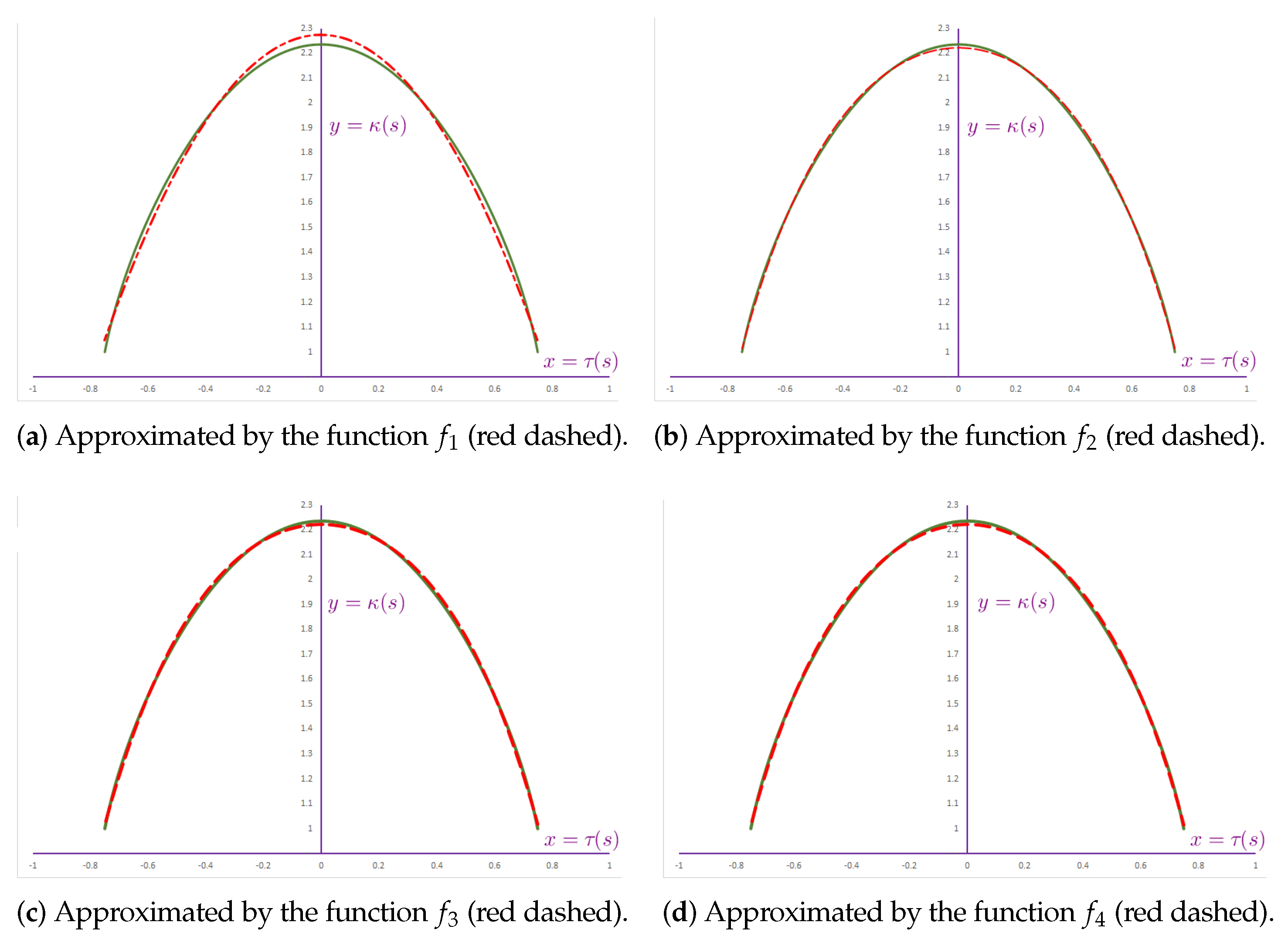
The authors declare no conflicts of interest.

Appendix A

In this section, the discussion is focused on the curvatures of Viviani’s curve. First, we derive an explicit formula for the two curvatures of the curve such as κ = f ( τ ) . Then, we try to approximate the function f by using the ordinary least square (OLS) method. As can be followed from Figure 2b provided in Section 1, a relative relation between the curvatures of Viviani’s curve has a concave functional form where the maximum is reached at ( τ , κ ) s = π = ( 0 , 5 ) . Therefore, to establish a best approximation, we choose the following similar concave functional forms which can be found in [1,2]:
  • Quadratic (parabolic curve) κ ^ = f 1 ( τ ) = a 1 τ 2 + a 2 τ + a 3 ;
  • Exponential (normal (bell) curve ) κ ^ = f 2 ( τ ) = b 1 e b 2 τ 2 + b 3 ;
  • Hyperbolic (Catenary’s chain curve) κ ^ = f 3 ( τ ) = c 1 cosh c 2 τ + c 3 ;
  • Rational (Gutschoven’s kappa curve) κ ^ = f 4 ( τ ) = d 1 τ 2 d 2 τ 2 + d 3 .
Let us examine the relationship between the two curvatures defined in (8) and (9). Upon solving the relation (9) for c o s ( s ) , we have two roots, which are given in the following:
cos 1 ( s ) = 3 9 15 τ ( s ) 2 3 τ ( s ) s = arccos 3 9 15 τ ( s ) 2 3 τ ( s ) .
Note that, for every τ ( s ) R , the range of the second root of the solution, which is cos 2 ( s ) = 3 + 9 15 τ ( s ) 2 3 τ ( s ) , falls into the outside of the domain of the arccos function, which is [ 1 , 1 ] . Therefore, we will omit this second root.
Next, by substituting (A1) into (8), we can provide the explicit form for the relation of the two curvatures as follows:
κ ( s ) = 3 3 2 τ ( s ) 2 3 9 15 τ ( s ) 2 3 9 15 τ ( s ) 2 τ ( s ) 2 3 2 ,
where 0.75 τ ( s ) 0.75 and 1 κ ( s ) 5 .
The best method to fit a given data set to a functional form is the ordinary least squares (OLS) method. The goal is to estimate the coefficients of the approximation function that minimizes the sum of the squared differences between the observed real data and the approximated data [39]. In our case, the data are created with the curvature κ ( s ) and torsion τ ( s ) of Viviani’s curve for n = 1000 equally spaced points of the interval s [ 0 , π ] . Therefore, the objective function can be written as
a r g m i n a , b , c , d 1 , 2 , 3 i = 1 n κ i f j ( τ i ) 2 ,
where j = 1 , , 4 corresponds to the different functional forms. The table below provides the OLS estimates of the coefficients and the corresponding fit indexes (see also Figure A1).
Figure A1. Approximation to the curve r ( s ) = ( τ ( s ) , κ ( s ) ) (green solid) by different functions f j , ( j = 1 , , 4 ) .
Mathematics 13 01526 g0a1
According to the results provided in Table A1, the best fit indexes were obtained by the function f 4 , which is known to be Gutschoven’s kappa-like curve. Other estimates can also be utilized for different purposes. For example, a curve whose curvatures have an exact quadratic relation can be studied by screening the parametric form of Viviani’s curve or some other of its tuning forms. It is also worth noting that the gnomonic projection of Viviani’s curve corresponds to Gutschoven’s kappa-like curve as well.
Table A1. Approximation to the curve r ( s ) = ( τ ( s ) , κ ( s ) ) by four different functional forms.
Functional FormApproximated Function with OLS Estimated CoefficientsSSE R 2 RMSE
Quadratic κ ^ = f 1 ( τ ) = 2.18 * τ 2 + 0.000 τ + 2.274 * 10.10.99450.032
Exponential κ ^ = f 2 ( τ ) = 1.509 * e 1.045 * τ 2 + 3.731 * 1.1120.99940.011
Hyperbolic κ ^ = f 3 ( τ ) = 0.4439 * cosh 2.649 * τ + 2.666 1.2170.99930.011
Rational (the best approx.) κ ^ = f 4 ( τ ) = 1.867 * τ 2 1.315 * τ 2 + 2.224 * 0.7910.99960.009
(*): coefficient is significant at 0.01 level, SSE: sum of squares due to error, R 2 : the proportion of variance explained by the fit, RMSE: Root Mean Squared Error. Note: A value of SSE or RMSE closer to zero and a value of R 2 closer to 1 mean a better fit.

References

  1. Lawrence, J.D. A Catalog of Special Plane Curves; Courier Corporation: Chelmsford, MA, USA, 2013. [Google Scholar]
  2. Gray, A. Modern Differential Geometry of Curves and Surfaces with Mathematica, 2nd ed.; CRC: Boca Raton, FL, USA, 1997. [Google Scholar]
  3. Havil, J. Curves for the Mathematically Curious; Princeton University Press: Princeton, NJ, USA, 2019. [Google Scholar]
  4. Zhao, X.; Pei, D. Evolutoids of the Mixed-Type Curves. Adv. Math. Phy. 2021, 2021, 9330963. [Google Scholar] [CrossRef]
  5. Castro, I.; Castro-Infantes, I.; Castro-Infantes, J. New plane curves with curvature depending on distance from the origin. Mediterr. J. Math. 2017, 14, 1–19. [Google Scholar] [CrossRef]
  6. Izumiya, S.; Takeuchi, N. Evolutoids and pedaloids of plane curves. Note Mat. 2019, 39, 13–23. [Google Scholar]
  7. Struik, D.J. Lectures on Classical Differential Geometry; Courier Corporation: Chelmsford, MA, USA, 1961. [Google Scholar]
  8. Bertrand, J. Mémoire sur la théorie des courbes à double courbure. J. Math. Pures Appl. 1850, 15, 332–350. [Google Scholar]
  9. Mannheim, A. De l’emploi de la courbe représentative de la surface des normales principales d’une courbe gauche pour la démonstration de propriétés relatives à cette courbure. C. R. Comptes Rendus Séances l’Acad. Sci. 1878, 86, 1254–1256. [Google Scholar]
  10. Salkowski, E. Zur transformation von raumkurven. Math. Ann. 1909, 66, 517–557. [Google Scholar] [CrossRef]
  11. Monterde, J. Salkowski curves revisited: A family of curves with constant curvature and non-constant torsion. Comput. Aided Geom. Des. 2009, 26, 271–278. [Google Scholar] [CrossRef]
  12. Choi, J.H.; Kim, Y.H. Associated curves of a Frenet curve and their applications. Appl. Math. Comput. 2012, 218, 9116–9124. [Google Scholar] [CrossRef]
  13. Nurkan, S.K.; Güven, İ.A.; Karacan, M.K. Characterizations of adjoint curves in Euclidean 3-space. Proc. Natl. Acad. Sci. India Sect. A Phys. Sci. 2019, 89, 155–161. [Google Scholar] [CrossRef]
  14. Deshmukh, S.; Chen, B.Y.; Alghanemi, A. Natural mates of Frenet curves in Euclidean 3-space. Turk. J. Math. 2018, 42, 2826–2840. [Google Scholar] [CrossRef]
  15. Caddeo, R.; Montaldo, S.; Piu, P. The Mobius strip and Viviani’s windows. Math. Intell. 2001, 23, 36–40. [Google Scholar] [CrossRef]
  16. Ferreol, R. Viviani Curve. Available online: https://mathcurve.com/courbes3d.gb/viviani/viviani.shtml (accessed on 1 April 2023).
  17. Goemans, W.; de Woestyne, I.V. Clelia curves, twisted surfaces and Plücker’s conoid in Euclidean and Minkowski 3-space. In Recent Advances in the Geometry of Submanifolds: Dedicated to the Memory of Franki Dillen (1963–2013); American Mathematical Society: Providence, RI, USA, 2016; Volume 674, p. 59. [Google Scholar]
  18. Taner, T. Geometry of Spherical Viviani’s Curves in R 3 1 Lorentz-Minkowski 3-Space. Unpublished Doctoral Thesis, The Institute of Science, Manisa Celal Bayar University, Manisa, Türkiye, 2021. [Google Scholar]
  19. Graefe, E.M.; Korsch, H.J.; Strzys, M.P. Bose–Hubbard dimers, Viviani’s windows and pendulum dynamics. J. Phys. Math. Theor. 2014, 47, 085304. [Google Scholar] [CrossRef]
  20. Song, X.; Pei, D. Dual framed surfaces of traveling trajectories of geometrical particles. Mod. Phys. Lett. A 2025, 2025, 2550002. [Google Scholar] [CrossRef]
  21. Li, P.; Pei, D. Nullcone fronts of spacelike framed curves in Minkowski 3-space. Mathematics 2021, 9, 2939. [Google Scholar] [CrossRef]
  22. Zhu, M.; Yang, H.; Li, Y.; Abdel-Baky, R.A.; Al-Jedani, A.; Khalifa, M. Directional developable surfaces and their singularities in Euclidean 3-space. Filomat 2024, 38, 11333–11347. [Google Scholar]
  23. Li, Y.; Eren, K.; Ersoy, S.; Savic, A. Modified Sweeping Surfaces in Euclidean 3-Space. Axioms 2024, 13, 800. [Google Scholar] [CrossRef]
  24. Zhu, Y.; Li, Y.; Eren, K.; Ersoy, S. Sweeping Surfaces of Polynomial Curves in Euclidean 3-space. An. St. Univ. Ovidius Constanta 2025, 33, 293–311. [Google Scholar]
  25. Aldossary, M.T.; Abdel-Baky, R.A. Sweeping surface due to rotation minimizing Darboux frame in Euclidean 3-space E3. AIMS Math. 2022, 8, 447–462. [Google Scholar] [CrossRef]
  26. Li, Y.; Mallick, A.K.; Bhattacharyya, A.; Stankovic, M.S. A Conformal η-Ricci Soliton on a Four-Dimensional Lorentzian Para-Sasakian Manifold. Axioms 2024, 13, 753. [Google Scholar] [CrossRef]
  27. Li, Y.; Bouleryah, M.L.H.; Ali, A. On Convergence of Toeplitz Quantization of the Sphere. Mathematics 2024, 12, 3565. [Google Scholar] [CrossRef]
  28. Honda, S.; Takahashi, M. Framed curves in the Euclidean space. Adv. Geom. 2016, 16, 265–276. [Google Scholar] [CrossRef]
  29. Fukunaga, T.; Takahashi, M. Existence conditions of framed curves for smooth curves. J. Geom. 2017, 108, 763–774. [Google Scholar] [CrossRef]
  30. Huang, J.; Pei, D. Singularities of Non-Developable Surfaces in Three-Dimensional Euclidean Space. Mathematics 2019, 7, 1106. [Google Scholar] [CrossRef]
  31. Li, Y.; Siddesha, M.S.; Kumara, H.A.; Praveena, M.M. Characterization of Bach and Cotton Tensors on a Class of Lorentzian Manifolds. Mathematics 2024, 12, 3130. [Google Scholar] [CrossRef]
  32. Cao, L.; Xu, G.; Dai, Z. A New Characterization of totally umbilical hypersurfaces in de Sitter space. Adv. Pure Math. 2014, 4, 42–46. [Google Scholar] [CrossRef]
  33. Li, Y.; Bin-Asfour, M.; Albalawi, K.S.; Guediri, M. Spacelike Hypersurfaces in de Sitter Space. Axioms 2025, 14, 155. [Google Scholar] [CrossRef]
  34. Smarandache, F. Mixed noneuclidean geometries. arXiv 1991, arXiv:math/0010119. [Google Scholar]
  35. Mao, L.F. Smarandache Multi-Space Theory. In Partially Post-Doctoral Research for the Chinese Academy of Sciences; HEXIS: Phoenix, AZ, USA, 2006. [Google Scholar]
  36. Turgut, M.; Yılmaz, S. Smarandache Curves in Minkowski Spacetime. Int. J. Math. Comb. 2008, 3, 51–55. [Google Scholar]
  37. Ali, A.T. Special Smarandache curves in the Euclidean space. Int. J. Math. Comb. 2010, 2, 30–36. [Google Scholar]
  38. Do-Carmo, P. Differential Geometry of Curves and Surfaces; IMPA: London, UK; Prentice-Hall, Inc.: Englewood Cliffs, NJ, USA, 1976. [Google Scholar]
  39. Montgomery, D.C.; Peck, E.A.; Vining, G.G. Introduction to Linear Regression Analysis; John Wiley & Sons: Hoboken, NJ, USA, 2021. [Google Scholar]
  40. Abdel-Aziz, H.S.; Saad, M.K. Computation of Smarandache curves according to Darboux frame in Minkowski 3-space. J. Egypt. Math. Soc. 2017, 25, 382–390. [Google Scholar] [CrossRef]
  41. Bektaş, Ö.; Yüce, S. Special Smarandache Curves According to Darboux Frame in E3. Rom. J. Math. Comput. Sci. 2013, 3, 48–59. [Google Scholar]
  42. Çalışkan, A.; Şenyurt, S. Smarandache curves in terms of Sabban frame of spherical indicatrix curves. Gen. Math. Notes 2015, 31, 1–15. [Google Scholar]
  43. Çetin, M.; Tuncer, Y.; Karacan, M.K. Smarandache curves according to Bishop frame in Euclidean 3-space. Gen. Math. Notes 2014, 20, 50–66. [Google Scholar]
  44. Çetin, M.; Kocayigit, H. On the quaternionic Smarandache curves in Euclidean 3-space. Int. J. Contemp. Math. Sci. 2013, 8, 139–150. [Google Scholar] [CrossRef]
  45. Elzawy, M.; Mosa, S. Smarandache curves in the Galilean 4-space G4. J. Egypt. Math. Soc. 2017, 25, 53–56. [Google Scholar] [CrossRef]
  46. Gürses, N.B.; Bektaş, O.; Yüce, S. Special Smarandache curves in R31. Commun. Fac. Sci. Univ. Ank. Ser. A1 Math. Stat. 2016, 65, 143–160. [Google Scholar] [CrossRef]
  47. Kahraman, T.; Uğurlu, H. Dual smarandache curves and smarandache ruled surfaces. Math. Sci. Appl. E-Notes 2014, 2, 83–98. [Google Scholar]
  48. Ozturk, E.B.K.; Ozturk, U.; İlarslan, K.; Nešović, E. On pseudohyperbolical Smarandache curves in Minkowski 3-space. Int. J. Math. Math. Sci. 2013, 2013, 658–670. [Google Scholar] [CrossRef]
  49. Saad, M.K. Spacelike and timelike admissible Smarandache curves in pseudo-Galilean space. J. Egypt. Math. Soc. 2016, 24, 416–423. [Google Scholar] [CrossRef]
  50. Taşköprü, K.; Tosun, M. Smarandache Curves on S2. Bol. Soc. Parana. Mat. 3 Srie 2014, 32, 51–59. [Google Scholar] [CrossRef]
  51. The University of New Mexico. Smarandache Geometries. Available online: https://fs.unm.edu/SG/ (accessed on 3 April 2025).
Figure 1. The special Viviani’s curve (purple) as an intersection of a cylinder (blue) and sphere (red) where π s π .
Mathematics 13 01526 g001
Figure 2. The graphs for the curvature functions of Viviani’s curve, where s [ 2 π , 2 π ] .
Mathematics 13 01526 g002
Figure 3. The T N Smarandache curve of Viviani’s curve, π s π .
Mathematics 13 01526 g003
Figure 4. The curvatures of the T N Smarandache curve of Viviani’s curve.
Mathematics 13 01526 g004
Figure 5. The N B Smarandache curve of Viviani’s curve, π s π .
Mathematics 13 01526 g005
Figure 6. The curvatures of the N B Smarandache curve of Viviani’s curve.
Mathematics 13 01526 g006
Figure 7. The T B Smarandache curve of Viviani’s curve, π s π .
Mathematics 13 01526 g007
Figure 8. The curvatures of the T B Smarandache curve of Viviani’s curve.
Mathematics 13 01526 g008
Figure 9. The T N B Smarandache curve of Viviani’s curve, π s π .
Mathematics 13 01526 g009
Figure 10. The curvatures of the T N B Smarandache curve of Viviani’s curve.
Mathematics 13 01526 g010
Figure 11. The N C Smarandache curve of Viviani’s curve, π s π .
Mathematics 13 01526 g011
Figure 12. The curvatures of the N C Smarandache curve of Viviani’s curve.
Mathematics 13 01526 g012
Figure 13. The T C Smarandache curve of Viviani’s curve, π s π .
Mathematics 13 01526 g013
Figure 14. The curvatures of the T C Smarandache curve of Viviani’s curve.
Mathematics 13 01526 g014
Figure 15. The B C Smarandache curve of Viviani’s curve, π s π .
Mathematics 13 01526 g015
Figure 16. The curvatures of the B C Smarandache curve of Viviani’s curve.
Mathematics 13 01526 g016
Disclaimer/Publisher’s Note: The statements, opinions and data contained in all publications are solely those of the individual author(s) and contributor(s) and not of MDPI and/or the editor(s). MDPI and/or the editor(s) disclaim responsibility for any injury to people or property resulting from any ideas, methods, instructions or products referred to in the content.

