Multivariate Extension Application for Spearman’s Footrule Correlation Coefficient

Abstract

This paper presents a simplified and computationally feasible multivariate extension. A correlation matrix is constructed using pairwise Spearman’s footrule correlation coefficients, and these coefficients are shown to jointly converge to a multivariate normal distribution. A global test statistic based on the Frobenius norm of this matrix asymptotically follows a weighted sum of chi-square distributions. Simulation studies and two real-world applications (a sensory analysis of French Jura wines and the characterization of plant leaf specimens) demonstrate the practical utility of the proposed method, bridging the gap between theoretical rigor and practical implementation in multivariate nonparametric inference.

1. Introduction

Nonparametric association measures serve as indispensable tools in statistical analysis, especially when handling non-Gaussian distributions or intricate dependence structures. Spearman’s footrule rank correlation coefficient [1], a rank-based statistic, has recently regained prominence for its resilience to parametric assumptions and ease of interpretation [2,3,4]. By aggregating absolute differences between paired ranks, this metric captures permutation-based disorder while circumventing limitations of linear correlation measures like Spearman’s rho correlation coefficient.

Four key attributes solidify Spearman’s footrule as a versatile analytical instrument: (i) computational efficiency ($O\left(n\right)$ complexity), surpassing quadratic-time alternatives like Kendall’s tau; (ii) sensitivity to positional deviations, crucial for applications prioritizing top-ranked items; (iii) intuitive interpretation through normalized rank displacement metrics; and (iv) enhanced outlier resistance compared to Euclidean-based counterparts. These properties enable diverse applications: genomic reproducibility analysis under noisy conditions [5], ranked list comparison in information retrieval [6,7], and uncertainty-aware consensus ranking in preference learning [8]. Its adaptability further extends to gene expression studies [9] and bioinformatics workflows [10], demonstrating broad interdisciplinary utility.

Recent decades have witnessed considerable efforts to extend Spearman’s footrule to multivariate contexts. Úbeda-Flores (2005) [11] introduced a copula-based multivariate generalization that preserves interpretability, though its computational complexity limits its practical utility. Genest et al. (2010) [12] further analyzed the theoretical properties of Spearman’s footrule and Gini’s gamma, emphasizing persistent challenges in developing efficient multivariate tests and establishing tight bounds. While the range of the lower bound was theoretically established, the complete characterization of copulas achieving this range remained unresolved until [13] identified sparse copula structures attaining its minimum value.

Despite these advancements, significant limitations persist. Current multivariate extensions of Spearman’s footrule, while theoretically robust, often depend on intricate copula formulations (e.g., [11,14]), compromising their accessibility and practical implementation. To address this gap, we propose a novel multivariate testing approach prioritizing simplicity and computational feasibility. Our approach begins by constructing a $p\times q$ correlation matrix through pairwise computation of Spearman’s footrule coefficients between all components of two p- and q-dimensional random vectors. This matrix encapsulates rank-based dependencies in a structure analogous to classical correlation matrices. We formally demonstrate that, under independence assumptions, its elements jointly converge to a multivariate normal distribution using the Cramér–Wold device and asymptotic representation techniques, thereby extending univariate normality results to multivariate settings. A global test statistic derived from the Frobenius norm of this matrix asymptotically follows a weighted sum of chi-square distributions. However, recognizing the impracticality of critical value tabulation for this complex distribution, we recommend a permutation-based testing procedure. This method empirically approximates the null distribution, offering enhanced robustness and scalability in finite-sample applications.

Simulation studies confirm that the permutation approach maintains well-controlled Type I error rates and demonstrates superior power compared to existing methods, while applications to two real-world datasets illustrate its practical effectiveness in detecting dependencies. This work bridges the gap between theoretical development and pragmatic implementation, providing a scalable and robust framework for multivariate nonparametric inference.

The remaining sections are organized as follows: Section 2 formally introduces the multivariate footrule correlation matrix, establishes its joint asymptotic normality, and outlines the permutation-based testing procedure. Section 3 and Section 4 evaluate the method through simulations and real-data demonstrations, respectively, while Section 5 concludes with a discussion of implications and potential extensions. Technical proofs are deferred to Appendix A and Appendix B to provide additional simulations for covariance estimation. The codes implementing the simulation studies are available online.

2. Multivariate Extension of Independence Test

Consider two real-valued, continuous random vectors, $\mathit{X}={(X_1,\cdots ,X_p)}^{\top }\in {\mathbb{R}}^p$ and $\mathit{Y}={(Y_1,\cdots ,Y_q)}^{\top }\in {\mathbb{R}}^q$, with fixed dimensions of p and q, respectively. Suppose n independent and identically distributed (i.i.d.) observations ${\left({\mathit{X}}_1^{\top },{\mathit{Y}}_1^{\top }\right)}^{\top },\dots ,{\left({\mathit{X}}_n^{\top },{\mathit{Y}}_n^{\top }\right)}^{\top }$ are from ${({\mathit{X}}^{\top },{\mathit{Y}}^{\top })}^{\top }$, where ${\mathit{X}}_i={(X_{i1},\cdots ,X_{ip})}^{\top }$, ${\mathit{Y}}_i={(Y_{i1},\cdots ,Y_{iq})}^{\top }$ for $i=1,\cdots ,n$.

We begin by revisiting the bivariate Spearman’s footrule. For a sample $\{{(X_{1k},Y_{1l})}^{\top },\cdots ,{(X_{nk},Y_{nl})}^{\top }\}$ from the paired variables $(X_k,Y_l)$ with their marginal distribution functions $F_k$ and $G_l$ ($1⩽k⩽p,1⩽l⩽q$), let $R_{ik}={\sum }_{j=1}^n\mathbb{I}\left(X_{jk}⩽X_{ik}\right)$ and $S_{il}={\sum }_{j=1}^n\mathbb{I}\left(Y_{jl}⩽Y_{il}\right)$ denote the ranks of $X_{ik}$ and $Y_{il}$, respectively. The bivariate Spearman’s footrule, tailored for the two scalars, $X_k$ and $Y_l$, is then given by the following expression:

$$\begin{array}{c}\hfill {\phi }_{kl}:={\phi }_n\left({\left\{{(X_{ik},Y_{il})}^{\top }\right\}}_{i=1}^n\right)=1-{\displaystyle \frac{3}{n^2-1}}\sum _{i=1}^n\left|R_{ik}-S_{il}\right|.\end{array}$$

(1)

Thus, based on Equation (1), the Spearman’s footrule correlation matrix applied to vectors $\mathit{X}$ and $\mathit{Y}$ can be defined as

$$\mathbf{M}:=\left(\begin{array}{cccc}{\phi }_{11}& {\phi }_{12}& \cdots & {\phi }_{1q}\\ {\phi }_{21}& {\phi }_{22}& \cdots & {\phi }_{2q}\\ ⋮& ⋮& \ddots & ⋮\\ {\phi }_{p1}& {\phi }_{p2}& \cdots & {\phi }_{pq}\end{array}\right).$$

In this study, we will concentrate on the utilization of $\mathbf{M}$ in conducting independence tests. To be specific, we will explore the following null and alternative hypotheses based on n i.i.d. observations.

$$\begin{array}{c}\hfill H_0:\mathit{X}\mathrm{and}\mathit{Y}\mathrm{are}\mathrm{independent}⟷H_1:\mathit{X}\mathrm{and}\mathit{Y}\mathrm{are}\mathrm{dependent}.\end{array}$$

(2)

For ease of notation, we denote the set of observations as ${\mathcal{D}}_n=\left\{{\left({\mathit{X}}_1^{\top },{\mathit{Y}}_1^{\top }\right)}^{\top },\dots ,{\left({\mathit{X}}_n^{\top },{\mathit{Y}}_n^{\top }\right)}^{\top }\right\}$. To examine Equation (2), the multivariate Spearman’s footrule rank test statistic, which is obtained by aggregating the $pq$ squared and standardized bivariate Spearman’s footrules from the correlation matrix $\mathbf{M}$, takes the specific form

$$\begin{array}{c}\hfill T_n:=T_n\left({\mathcal{D}}_n\right)=u_n^{-1}{\left|\right|\mathbf{M}\left|\right|}_F^2,\end{array}$$

(3)

where $u_n={\displaystyle \frac{2n^2+7}{5(n+1){(n-1)}^2}}$ is the variance of ${\phi }_{kl}$ under the independence assumption, which can be directly calculated using the results from [15]. The notation $\left|\right|·{\left|\right|}_F$ represents the Frobenius norm of a matrix; specifically, for a $p\times q$ matrix $\mathbf{A}$ with elements $A_{kl}$ and $k=1,\cdots ,p,l=1,\cdots ,q$, the Frobenius norm is computed as ${\left|\right|\mathbf{A}\left|\right|}_F=\sqrt{{\sum }_{k=1}^p{\sum }_{l=1}^q{A}_{kl}^2}$.

Furthermore, for any $p\times q$ matrix $\mathbf{A}$, $\mathbf{vec}\left(\mathbf{A}\right)$ is employed to denote the $pq\times 1$ column vector by vertically stacking the columns of matrix $\mathbf{A}$. The theorem presented below provides the asymptotic joint normality property of the elements in matrix $\mathit{M}$.

Theorem 1. 

Under the null hypothesis $H_0$, $\sqrt{n}\mathbf{vec}\left(\mathbf{M}\right)$ converges in distribution to a $pq$-dimensional multivariate normal distribution with mean vector $\mathbf{0}$ and covariance matrix Σ, i.e., as $n\to \infty$,

$$\begin{array}{c}\hfill \sqrt{n}\mathbf{vec}\left(\mathbf{M}\right)\stackrel{d}{\to }{N}_{pq}\left(\mathbf{0},\mathbf{\Sigma }\right).\end{array}$$

In the covariance matrix Σ, the diagonal entries are all equal to $2/5$, whereas the off-diagonal elements are determined by $9\mathrm{E}\left(W_1^{kl}{W}_1^{rs}\right)$, given that $W_1^{kl}=|U_{1k}-V_{1l}|+U_{1k}(1-U_{1k})+V_{1l}(1-V_{1l})-{\displaystyle \frac{2}{3}}$ with $U_{1k}=F_k\left(X_{1k}\right)$ and $V_{1l}=G_l\left(Y_{1l}\right)$ for $1⩽k,r⩽p,1⩽l,s⩽q$, $(k,l)\ne (r,s)$.

The derivation of Theorem 1 primarily relies on the Hájek asymptotic representation of the following form presented in [16]:

$$\begin{array}{c}\hfill {\tilde{\phi }}_{kl}=-{\displaystyle \frac{3}{n+1}}\sum _{i=1}^n\left(|U_{ik}-V_{il}|+U_{ik}(1-U_{ik})+V_{il}(1-V_{il})-{\displaystyle \frac{2}{3}}\right)\end{array}$$

(4)

where ${\tilde{\phi }}_{kl}$ is asymptotically equidistributed with ${\phi }_{kl}$ when $X_k$ and $X_l$ are independent, and it effectively removes the dependence among ranks, greatly facilitating the further development of the theory.

For the plug-in estimation of covariance matrix  $\mathbf{\Sigma }$, one may substitute the expectation of off-diagonal elements in $\mathbf{\Sigma }$ with corresponding sample means and replace the population distribution function with the corresponding empirical distribution function. The resulting estimator $\widehat{\mathbf{\Sigma }}$ has the following specific form: diagonal elements equal 2/5, and off-diagonal elements equal ${\displaystyle \frac{9}{n}}{\sum }_{i=1}^n\widehat{W_i^{kl}}\widehat{W_i^{rs}}$ for $1⩽k,r⩽p,1⩽l,s⩽q$, $(k,l)\ne (r,s)$, where

$$\widehat{W_i^{kl}}=|F_k^n\left(X_{ik}\right)-G_l^n\left(Y_{il}\right)|+F_k^n\left(X_{ik}\right)(1-F_k^n\left(X_{ik}\right))+G_l^n\left(Y_{il}\right)(1-G_l^n\left(Y_{il}\right))-{\displaystyle \frac{2}{3}}.$$

$F_k^n$ and $G_l^n$ denote the empirical distribution functions of $X_k$ and $X_l$, respectively, defined as $F_k^n\left(x\right)={\displaystyle \frac{1}{n}}{\sum }_{i=1}^n\mathbb{I}\left(X_{ik}⩽x\right)$ and $G_l^n\left(y\right)={\displaystyle \frac{1}{n}}{\sum }_{i=1}^n\mathbb{I}\left(Y_{il}⩽y\right)$. The performance of this estimator is demonstrated through simulations in Appendix B, which reveal that practical within-group dependencies and sample size significantly impact estimation accuracy. Consequently, we employ the random permutation technique (described later) when conducting hypothesis tests in real applications.

By leveraging the joint normality property of all elements within $\mathbf{\Sigma }$, as established by Theorem 1, we can readily derive the asymptotic null distribution of the multivariate Spearman’s footrule statistic.

Corollary 1. 

Under the null hypothesis $H_0$, as $n\to \infty$,

$$\begin{array}{c}\hfill {\displaystyle \frac{2}{5}}{T}_n\stackrel{d}{\to }\sum _{k=1}^{pq}{\lambda }_k{Z}_k^2,\end{array}$$

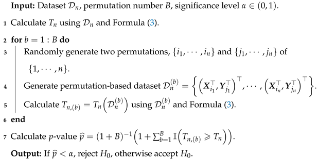
where ${\lambda }_k$ represents the eigenvalues of matrix Σ, and $Z_k$ for $k=1,\cdots ,pq$ are independent standard normal random variables.

Although Corollary 1 furnishes the asymptotic result for determining the critical values of the proposed test statistic, the unknown joint distribution of every pair of components within $\mathit{X}$ or $\mathit{Y}$ complicates the intricate expectations in covariance matrix $\mathbf{\Sigma }$ and renders the task of finding suitable estimates challenging. Although the commonly used plug-in estimation technique can serve as an alternative estimation method, its performance is susceptible to both the sample size and the complex within-group dependencies. Consequently, the critical values derived in Corollary 1 are impractical and cannot serve as valid critical values for the testing procedure. To address this issue, we can employ random permutation to conduct the test. The specific procedure and algorithm (Algorithm 1) are outlined as follows:

Step 1:

Given the dataset of observations ${\mathcal{D}}_n=\left\{{\left({\mathit{X}}_1^{\top },{\mathit{Y}}_1^{\top }\right)}^{\top },\dots ,{\left({\mathit{X}}_n^{\top },{\mathit{Y}}_n^{\top }\right)}^{\top }\right\},$ specify the number of permutations, denoted as B.

Step 2:

For each $b\in \{1,\cdots ,B\}$, randomly generate two permutations, $\{i_1,\cdots ,i_n\}$ and $\{j_1,\cdots ,j_n\}$, of the index set $\{1,\cdots ,n\}$.

Step 3:

Construct the b-th permuted dataset ${\mathcal{D}}_n^{\left(b\right)}=\left\{{\left({\mathit{X}}_{i_1}^{\top },{\mathit{Y}}_{j_1}^{\top }\right)}^{\top },\cdots ,{\left({\mathit{X}}_{i_n}^{\top },{\mathit{Y}}_{j_n}^{\top }\right)}^{\top }\right\}$ based on the generated permutations.

Step 4:

Calculate the b-th permutation-based statistics $T_{n,\left(b\right)}=T_n\left({\mathcal{D}}_n^{\left(b\right)}\right)$ using the permuted dataset.

Step 5:

Repeat Steps 2–4 B times. Utilize the collection of statistics $\{T_{n,\left(1\right)},\cdots ,T_{n,\left(B\right)}\}$ to approximate the p-value of the test as follows:

$$\begin{array}{c}\hfill \widehat{p}={(1+B)}^{-1}\left(1+\sum _{b=1}^B\mathbb{I}\left(T_{n,\left(b\right)}⩾T_n\right)\right).\end{array}$$

Step 6:

For a prespecified significance level $\alpha \in (0,1)$, if $\widehat{p}<\alpha$, reject the null hypothesis $H_0$.

3. Simulations

To evaluate the performance of the multivariate footrule test statistic proposed in this paper (denoted as Mfootrule and given in Equation (3)), we conduct a series of simulations in this section using four synthetic examples. These examples encompass 2 models for investigating the validity of tests under the null hypothesis, 12 models for examining the power, and 4 varying models designed to visualize the trend of test power when data are generated under the alternative hypothesis.

For the purpose of comparison, we select several commonly employed methods to test the independence of two multivariate vectors. These include distance covariance (DCOV) [17] and its marginal rank-based version (RDCOV) ([18]), the Hilbert–Schmidt Independence Criteria (HSIC) [19], along with two additional methods that bear similarity to the construction of our proposed statistic (they are, respectively, based on Spearman’s $\rho$ and Kendall’s $\tau$, as referenced in [20,21], denoted as Mrho and Mtau, respectively). All methods perform tests using permutation-based approaches with 1000 permutations, including our proposed method which specifically utilizes the permutation testing procedure described in Algorithm 1. Two sample sizes are set, $n=50$ and $n=100$, with dimensions of $p=q=3$. A significance level of 0.05 is set for all scenarios, with 1000 replicate simulations conducted. Detailed information on data generation can be found in the following four examples.    

Algorithm 1: Permutation-based algorithm for multivariate Spearman’s footrule test

Example 1 

(Data generated under $H_0$). In this example, in order to assess the validity of various testing methods, Gaussian distribution and non-Gaussian heavy-tailed distribution are employed to generate data under the null hypothesis. Additionally, we introduce within-group dependence to examine its impact on the empirical size of the tests. These two distributions are similar to the setups in Examples 6.1 and 6.2 of [22]. All of the empirical sizes are presented in

Table 1. The empirical size of various tests under $H_0$ in Example 1 with $\rho =0$.

	$\mathit{\tau }=0$	$\mathit{\tau }=0.1$	$\mathit{\tau }=0.2$	$\mathit{\tau }=0.3$	$\mathit{\tau }=0.4$	$\mathit{\tau }=0.5$	$\mathit{\tau }=0.6$	$\mathit{\tau }=0.7$	$\mathit{\tau }=0.8$	$\mathit{\tau }=0.9$
Gaussian distribution ($n=50$)
Mfootrule	0.045	0.038	0.052	0.057	0.069	0.053	0.054	0.042	0.056	0.057
Mrho	0.040	0.040	0.058	0.055	0.064	0.050	0.048	0.039	0.056	0.053
Mtau	0.046	0.035	0.054	0.055	0.063	0.052	0.046	0.042	0.054	0.056
RDCOV	0.043	0.031	0.057	0.049	0.058	0.052	0.055	0.045	0.059	0.053
DCOV	0.052	0.044	0.060	0.052	0.053	0.044	0.049	0.054	0.065	0.047
HSIC	0.050	0.037	0.060	0.056	0.053	0.042	0.048	0.054	0.053	0.051
Heavy-tailed distribution ($n=50$)
Mfootrule	0.044	0.038	0.049	0.056	0.068	0.050	0.053	0.044	0.058	0.055
Mrho	0.043	0.040	0.057	0.055	0.062	0.046	0.049	0.043	0.052	0.054
Mtau	0.042	0.036	0.060	0.057	0.059	0.050	0.046	0.039	0.052	0.057
RDCOV	0.044	0.036	0.056	0.047	0.056	0.054	0.052	0.049	0.059	0.056
DCOV	0.057	0.042	0.062	0.048	0.055	0.045	0.051	0.054	0.063	0.048
HSIC	0.048	0.043	0.058	0.052	0.056	0.044	0.048	0.057	0.056	0.048
Gaussian distribution ($n=100$)
Mfootrule	0.056	0.049	0.039	0.041	0.054	0.052	0.040	0.044	0.039	0.048
Mrho	0.052	0.041	0.040	0.048	0.056	0.047	0.039	0.044	0.043	0.050
Mtau	0.053	0.050	0.041	0.050	0.055	0.050	0.035	0.043	0.038	0.051
RDCOV	0.054	0.051	0.043	0.052	0.059	0.052	0.040	0.046	0.040	0.047
DCOV	0.050	0.054	0.048	0.045	0.058	0.053	0.047	0.048	0.044	0.054
HSIC	0.054	0.051	0.043	0.049	0.060	0.052	0.053	0.060	0.046	0.052
Heavy-tailed distribution ($n=100$)
Mfootrule	0.055	0.046	0.042	0.042	0.057	0.050	0.043	0.044	0.042	0.055
Mrho	0.050	0.042	0.039	0.049	0.056	0.044	0.042	0.045	0.042	0.048
Mtau	0.052	0.046	0.041	0.050	0.053	0.045	0.040	0.039	0.038	0.052
RDCOV	0.055	0.047	0.040	0.046	0.063	0.052	0.038	0.048	0.042	0.050
DCOV	0.049	0.055	0.044	0.049	0.060	0.053	0.045	0.047	0.044	0.053
HSIC	0.049	0.048	0.042	0.050	0.059	0.055	0.049	0.056	0.046	0.053

.

(a) 

(Gaussian) ${({\mathit{X}}^{\top },{\mathit{Y}}^{\top })}^{\top }={\left(X_1,\cdots ,X_p,Y_1,\cdots ,Y_q\right)}^{\top }$∼$N_{p+q}(\mathbf{0},\tilde{\mathbf{\Sigma }})$, where the entry ${\tilde{\mathrm{\Sigma }}}_{ij}$ of the covariance matrix $\tilde{\mathbf{\Sigma }}$ is defined as

$${\tilde{\Sigma }}_{ij}=\left\{\begin{array}{cc}\rho ,\hfill & \mathit{if}1⩽i⩽p,p+1⩽j⩽p+q\mathrm{or}p+1⩽i⩽p+q,1⩽j⩽p\hfill \\ 1,\hfill & \mathit{if}i=j\hfill \\ \tau ,\hfill & \mathit{otherwise}\hfill \end{array}\right.,$$

with $\tau \in [0,1]$ and $\rho \in [-1,1]$ representing the strengths of within-group and without-group dependence, respectively. In this model, data under the null hypothesis are generated by setting $\rho =0$ while allowing τ to vary.

(b) 

(Heavy-tail) Data generation is conducted independently from ${({\mathit{X}}^{\top },{\mathit{Y}}^{\top })}^{\top }$, such that the components of $\mathit{X}$ and $\mathit{Y}$ are given by $X_i=Q_{t\left(1\right)}\left(\Phi \left(X_i^{\ast }\right)\right)$ for $i=1,\cdots ,p$, and by $Y_j=Q_{t\left(1\right)}\left(\Phi \left(Y_j^{\ast }\right)\right)$ for $j=1,\cdots ,q$. In this context, $Q_{t\left(1\right)}$ represents the quantile function of the t-distribution with one degree of freedom, Φ is the cumulative distribution function of the standard Gaussian distribution, and ${\left({\mathit{X}}^{\ast \top },{\mathit{Y}}^{\ast \top }\right)}^{\top }={\left(X_1^{\ast },\cdots ,X_p^{\ast },Y_1^{\ast },\cdots ,Y_q^{\ast }\right)}^{\top }$ is generated in the same manner as described in Example 1(a).

From Table 1, it is evident that the proposed method, along with all of the methods employed for comparison, demonstrates good control over the empirical size across various levels of within-group dependence and different sample sizes, whether under Gaussian or heavy-tailed distributions. This is because both the proposed method and the comparative approaches utilize techniques based on random permutation or resampling to accurately estimate the null hypothesis distribution, thereby preventing distortion of the empirical size and confirming the validity of all tests.

Example 2 

(Data generated under $H_1$ in Example 1 with $\rho =0.2$). In this example, the data generation for the two models follows the same procedure as in Example 1(a) and Example 1(b), except that ρ is set to 0.2 to generate data under the alternative hypothesis.

The data presented in

Table 2. The empirical rejection rates of various tests under $H_1$ in Example 2 with $\rho =0.2$.

	$\mathit{\tau }=0$	$\mathit{\tau }=0.1$	$\mathit{\tau }=0.2$	$\mathit{\tau }=0.3$	$\mathit{\tau }=0.4$	$\mathit{\tau }=0.5$	$\mathit{\tau }=0.6$	$\mathit{\tau }=0.7$	$\mathit{\tau }=0.8$	$\mathit{\tau }=0.9$
Gaussian distribution ($n=50$)
Mfootrule	0.737	0.724	0.673	0.615	0.558	0.515	0.472	0.404	0.354	0.297
Mrho	0.783	0.752	0.716	0.633	0.576	0.523	0.479	0.407	0.362	0.307
Mtau	0.780	0.747	0.705	0.631	0.575	0.514	0.478	0.408	0.369	0.310
RDCOV	0.762	0.714	0.653	0.582	0.520	0.463	0.442	0.382	0.340	0.272
DCOV	0.831	0.756	0.700	0.614	0.555	0.493	0.445	0.396	0.337	0.294
HSIC	0.715	0.599	0.489	0.410	0.324	0.294	0.250	0.203	0.178	0.154
Heavy-tailed distribution ($n=50$)
Mfootrule	0.743	0.697	0.695	0.644	0.561	0.480	0.433	0.398	0.364	0.296
Mrho	0.795	0.748	0.711	0.657	0.592	0.494	0.438	0.398	0.375	0.324
Mtau	0.779	0.742	0.708	0.663	0.595	0.482	0.435	0.399	0.370	0.314
RDCOV	0.765	0.696	0.649	0.598	0.525	0.460	0.401	0.365	0.341	0.297
DCOV	0.113	0.114	0.127	0.091	0.110	0.116	0.091	0.117	0.105	0.089
HSIC	0.237	0.170	0.143	0.144	0.102	0.103	0.087	0.091	0.089	0.075
Gaussian distribution ($n=100$)
Mfootrule	0.974	0.966	0.939	0.914	0.862	0.791	0.717	0.642	0.553	0.510
Mrho	0.990	0.982	0.962	0.934	0.888	0.806	0.756	0.655	0.578	0.528
Mtau	0.988	0.982	0.961	0.930	0.893	0.805	0.754	0.658	0.578	0.544
RDCOV	0.983	0.969	0.938	0.907	0.849	0.762	0.711	0.610	0.540	0.483
DCOV	0.993	0.986	0.953	0.921	0.876	0.768	0.730	0.640	0.576	0.517
HSIC	0.973	0.933	0.840	0.763	0.642	0.552	0.459	0.369	0.308	0.264
Heavy-tailed distribution (n = 100)
Mfootrule	0.990	0.949	0.933	0.898	0.865	0.799	0.699	0.637	0.604	0.476
Mrho	0.997	0.980	0.950	0.917	0.891	0.835	0.722	0.667	0.620	0.512
Mtau	0.997	0.982	0.951	0.923	0.885	0.830	0.716	0.658	0.619	0.516
RDCOV	0.996	0.964	0.929	0.893	0.836	0.783	0.696	0.625	0.587	0.472
DCOV	0.154	0.170	0.161	0.115	0.123	0.127	0.134	0.118	0.118	0.115
HSIC	0.481	0.330	0.256	0.211	0.160	0.162	0.120	0.118	0.111	0.104

indicate that as the within-group dependence increases, all empirical rejection rates decrease, which is a normal phenomenon, since within-group dependence interferes with between-group dependence. Another notable observation is that all rank-based tests (including our proposed Mfootrule) demonstrate clear advantages under both Gaussian and heavy-tailed distributions. This is because rank-based tests, being insensitive to outliers, exhibit superior robustness in heavy-tailed distributions. Although our Mfootrule exhibits negligible disadvantages, these are inconsequential, especially considering that methods like Mrho and Mtau specialize in linear dependency detection for Gaussian models. In contrast, non-rank-based methods (DCOV and HSIC) perform poorly in heavy-tailed models due to their lack of robustness. The rank-based DCOV (RDCOV) also performs remarkably well but shows slight power loss compared to the original DCOV under Gaussian models, likely because it uses marginal ranks without fully accounting for interactions between within-group ranks. HSIC exhibits the lowest power in Gaussian models due to its limited linear dependency detection capability, and while it shows marginal advantages over DCOV in heavy-tailed models, its performance still lags behind our proposed methods and specialized linear dependency tests.

Example 3 

(Data generated from various general alternative models under $H_1$). In this example, additional general alternative models are generated to examine the capability of the proposed methods and the comparison methods in rejecting the null hypothesis. The construction involves ${({\mathit{X}}^{\top },{\mathit{Y}}^{\top })}^{\top }={\left(X_1,X_2,X_3,Y_1,Y_2,Y_3\right)}^{\top }$, where ${\left(X_i,Y_i\right)}^{\top }\stackrel{\mathrm{i}.\mathrm{i}.\mathrm{d}.}{\sim }{(X,Y)}^{\top }\in \mathbb{R}\times \mathbb{R}$ for $i=1,2,3$. There are 10 specific models that generate the distribution of $(X,Y)$, and some of these distributions are also taken into account in [23] for testing the independence of two vectors. These distributions can be categorized into four types: the first type is distributions with heavy-tailed dependence (V1–V3), the second type is distributions where the dependence follows a Gaussian or non-Gaussian mixture (V4–V6), the third type exhibits noisy functional dependence (V7–V8), and the fourth type features shape-based dependence (V9–V10). The detailed model settings are as follows, and all of the results are presented in

Table 3. The empirical rejection rates of various tests under the different alternative models in Example 3.

	V1	V2	V3	V4	V5	V6	V7	V8	V9	V10
$n=50$
Mfootrule	0.894	0.699	0.637	0.617	0.169	0.331	0.137	0.609	0.185	0.301
Mrho	0.762	0.466	0.462	0.352	0.076	0.299	0.102	0.657	0.021	0.132
Mtau	0.790	0.523	0.493	0.428	0.113	0.306	0.108	0.661	0.013	0.196
RDCOV	0.784	0.526	0.500	0.322	0.128	0.285	0.448	0.612	0.060	0.139
DCOV	0.051	0.059	0.039	0.365	0.061	0.354	0.485	0.656	0.048	0.122
HSIC	0.352	0.075	0.063	0.315	0.059	0.344	0.805	0.540	0.087	0.172
$n=100$
Mfootrule	0.998	0.952	0.950	0.947	0.232	0.549	0.129	0.952	0.548	0.535
Mrho	0.982	0.766	0.758	0.664	0.077	0.514	0.097	0.969	0.016	0.120
Mtau	0.985	0.806	0.805	0.753	0.106	0.527	0.103	0.968	0.012	0.180
RDCOV	0.986	0.841	0.832	0.642	0.232	0.501	0.969	0.954	0.113	0.162
DCOV	0.050	0.050	0.054	0.670	0.063	0.572	0.978	0.965	0.070	0.152
HSIC	0.740	0.121	0.062	0.617	0.057	0.586	1.000	0.909	0.168	0.310

.

(V1) 

(Heavy-tailed): Let $V\sim N(0,1)$, $W_1\sim Cauchy(0,1)$, and $W_2\sim Cauchy(0,1)$. Then, $X=0.6W_1+V$ and $Y=0.6W_2+V$, with V, $W_1$, and $W_2$ being mutually independent.

(V2) 

(Heavy-tailed): Let $V\sim N(0,1)$, $W_1\sim Pareto(1,2)$, and $W_2\sim Pareto(1,1)$. Then, $X=W_1^2+V$ and $Y=W_2^2+V$, with V, $W_1$, and $W_2$ being mutually independent.

(V3) 

(Heavy-tailed): Let $V\sim N(0,1)$, $W_1\sim Pareto(1,1)$, and $W_2\sim Pareto(1,1)$. Then, $X=|V+W_1{|}^{1.5}$ and $Y=|V+W_2{|}^{1.5}$, with V, $W_1$, and $W_2$ being mutually independent.

(V4) 

(Mixture): Let $X\sim N(0,2),E\sim Ber\left(0.2\right)$, and $V\sim N(0,2)$. Then, $Y=(1-E)V+EX$, with X, E, and V being mutually independent.

(V5) 

(Mixture): Let $W\sim U(-1,1),W_1\sim U(0,1),W_2\sim U(0,1)$, and $A\sim Ber\left(0.5\right)$. Then, $V_1=W+0.1W_1$ and $V_2=4{\left(W^2-0.5\right)}^2+0.1W_2$. Finally, $X=V_1$ and $Y=A\times N(10,1)+(1-A)V_2$, with W, $W_1$, $W_2$, and A being mutually independent.

(V6) 

(Mixture): Let ${\left(U_1,U_2,U_3,V_1,V_2,V_3\right)}^{\top }\sim N_6(\mathbf{0},\mathbf{\Sigma })$ and ${\left(W_1,W_2,W_3,Z_1,Z_2,Z_3\right)}^{\top }\sim N_6(\mathbf{1},\mathbf{\Sigma }/2)$, where these two vectors are independent. The covariance matrix Σ has entries such that ${\mathbf{\Sigma }}_{ii}=1$ and ${\mathbf{\Sigma }}_{ij}=0.3$ if $i⩽3,j>3$ or $i>3,j⩽3$. Further, $A_1\sim Ber\left(0.5\right)$ and $A_2\sim Ber\left(0.3\right)$. Then, ${\left(X_1,X_2,X_3\right)}^{\top }\sim \left(1-A_1\right){\left(U_1,U_2,U_3\right)}^{\top }+A_1{\left(W_1,W_2,W_3\right)}^{\top }$ and ${\left(Y_1,Y_2,Y_3\right)}^{\top }\sim (1-\left.A_2\right){\left(V_1,V_2,V_3\right)}^{\top }+A_2{\left(Z_1,Z_2,Z_3\right)}^{\top }$.

(V7) 

(Quadratic function): Let $X\sim U(-1,1)$ and $ϵ\sim U(0,1)$. Then, $Y=0.5X^2+0.5ϵ$, with X and ϵ being independent.

(V8) 

(Fractional exponential function): Let $X\sim U(0,1)$ and $ϵ\sim N(0,1)$. Then, $Y=X^{1/4}+0.5ϵ$, with X and ϵ being independent.

(V9) 

(Semicircle): Let $V\sim U(0,1)$. Then, $X=sin\left(\pi V\right)$ and $Y=cos\left(\pi V\right)$.

(V10) 

(Two parabolas): Let $V\sim Ber\left(0.5\right)$. Then, $X\sim U(-1,1)$, $Y=V(X^2+U(0,1))/2+(1-V)(X^2+U(0,1))/2$, with V and X being independent.

According to the results in Table 3, except for Models V7 and V8, where our proposed test is less proficient (although Model V8 only shows a slight disadvantage), our Mfootrule test outperforms all competitors by a significant margin among the remaining eight models. Among the two tests based on classical coefficients across all models, the Mtau test slightly outperforms the Mrho test, which is reasonable given their well-established performance in the bivariate case.

In heavy-tailed models V1-V3, which differ from the Gaussian-transformed heavy-tailed models in Example 2, the DCOV-based test completely fails even with increased sample sizes, while the marginal rank-based RDCOV maintains robust performance. This reflects the inherent robustness of rank-based methods against heavy-tailed distributions. Our Mfootrule outperforms classical methods (Mrho and Mtau) due to its absolute distance property and rank-based advantage, whereas HSIC shows limited power only in Model V1 and fails entirely in V2–V3 compared to rank-based approaches. For mixture distributions in Models V4–V6, RDCOV retains moderate performance in V4 and V6. Notably, in Gaussian and non-Gaussian mixture models (V5), the remaining four tests (Mtau, Mrho, DCOV, HSIC) perform poorly. Some methods (Mrho, DCOV, HSIC) show no power improvement with larger samples, while Mfootrule demonstrates consistent advantages over competitors through its unique design. In the non-monotonic functional dependence model V7, classical rank-based coefficients (Mtau, Mrho) perform poorly, as expected—since they specialize in linear/monotonic relationships—but our method surprisingly outperforms them. Meanwhile, underperforming HSIC excels here, while RDCOV and DCOV show moderate performance. In the monotonic model V8, all tests perform adequately without notable differences. In the shape-dependent models V9–V10, our proposed method excels, whereas other approaches show minimal effectiveness. Even renowned methods (Mrho, Mrho, DCOV) demonstrate no power improvement with larger samples, or, at best, marginal gains, with only HSIC showing slight advantages.

Example 4 

(Data generated from four varying alternative models). In this example, we generate four varying models to examine the trend of test power for all methods as the between-group dependence changes. Here, we set the sample size to $n=100$, and the number of simulations to 500, with the other settings remaining the same as before. The specific data-generating models are as follows:

(a) 

(Gaussian) This model is identical to Example 1(a), but with $\tau =0$ and ρ varying from $-0.3$ to 0.3.

(b) 

(Heavy-tailed) This model is identical to Example 1(b), but with $\tau =0$ and ρ varying from $-0.3$ to 0.3.

(c) 

(Mixture) $X\sim N(0,2),E\sim Ber\left(0.2\right)$, and $V\sim N(0,2)$. Then, $Y=(1-E)V+EX+\lambda ϵ$, with X, E, and V being mutually independent. This model extends the mixture model V4 from Example 3, where λ is a noise parameter. A larger λ implies weaker dependence between $\mathit{X}$ and $\mathit{Y}$, with $ϵ\sim N(0,1)$ representing noise.

(d) 

(Semicircle) $V\sim U(0,1)$. Then, $X=sin\left(\pi V\right)$ and $Y=cos\left(\pi V\right)+0.2\lambda ϵ$. This model extends semicircular model V9 from Example 3, where λ is a noise parameter. A larger λ implies weaker dependence between $\mathit{X}$ and $\mathit{Y}$, with $ϵ\sim N(0,1)$ representing noise.

The power curves of the four models are displayed in Figure 1. As shown in Figure 1a, all methods exhibit nearly identical performance for the Gaussian model, though our Mfootrule and HSIC exhibit virtually imperceptible slight disadvantages. In the Gaussian-transformed heavy-tailed model of Figure 1b, all rank-based tests (including our proposed methods) demonstrate strong robustness, while non-rank-based DCOV and HSIC show inferior performance. These findings align with the results from Example 2. For the Gaussian mixture model in Figure 1c, our method outperforms all competitors, as Mfootrule’s absolute difference-based distance metric effectively captures the mixture signals. In the semicircular model of Figure 1d, all tests exhibit extremely low power, whereas our method maintains a clear lead, with power degradation remaining gradual even as between-group dependency increases.

4. Real Data

In this section, we utilize two real-world datasets to demonstrate the performance of our proposed method. Unless otherwise specified, we maintain the same settings as in the previous section.

4.1. Sensory Analysis of French Jura Wines

This case study employs a methodological illustration from the domain of sensory analysis. Twelve trained panelists conducted duplicate evaluations (with an intersession interval of a few days) of eight Jura (France) wines using the Napping technique [24]. This innovative methodology requires participants to spatially arrange products on a standardized $60\times 40$ cm sheet based on perceived similarities (proximal placement) and dissimilarities (distal placement). Each session configuration generates an $8\times 2$ coordinate matrix per panelist–session combination, yielding 24 distinct matrices (12 panelists × two sessions). Such multidimensional data facilitate the investigation of perceptual stability in sensory evaluation.

To address the critical methodological question of panelist repeatability—specifically, whether individual perceptual configurations remain consistent across temporal sessions—we implemented all analytical procedures detailed in Section 3 under identical parameterization.

Table 4. p-values for all test methods assessing perceptual abilities of 12 panelists.

	Mfootrule	Mrho	Mtau	RDCOV	DCOV	HSIC
Panelist 1	0.005	0.161	0.107	0.206	0.093	0.164
Panelist 2	0.420	0.457	0.434	0.440	0.752	0.822
Panelist 3	0.323	0.130	0.227	0.206	0.311	0.449
Panelist 4	0.580	0.592	0.542	0.690	0.750	0.866
Panelist 5	0.481	0.432	0.415	0.362	0.020	0.024
Panelist 6	0.388	0.300	0.162	0.383	0.749	0.686
Panelist 7	0.001	0.001	0.001	0.001	0.008	0.007
Panelist 8	0.578	0.671	0.605	0.652	0.766	0.689
Panelist 9	0.118	0.250	0.313	0.293	0.126	0.259
Panelist 10	0.041	0.153	0.122	0.060	0.215	0.189
Panelist 11	0.550	0.463	0.747	0.431	0.258	0.221
Panelist 12	0.215	0.267	0.286	0.309	0.546	0.588

presents the comprehensive p-value matrix derived from these analyses. Notably, our proposed Mfootrule method demonstrated superior sensitivity in detecting perceptual stability, generating the smallest p-values for 7 of 12 panelists. However, given the limited interpretability of absolute p-value magnitudes, we conducted supplementary analyses across conventional significance levels ($\alpha =0.10,0.05,0.01$).

As evidenced in

Table 5. Rejection counts for testing perceptual ability among 12 panelists at different significance levels.

Level	Mfootrule	Mrho	Mtau	RDCOV	DCOV	HSIC
0.10	3	1	1	2	3	2
0.05	3	1	1	1	2	2
0.01	2	1	1	1	1	1

, the Mfootrule test exhibited the highest rejection counts across all significance levels, suggesting enhanced statistical power in identifying session-to-session perceptual consistency. This empirical outcome aligns with theoretical expectations regarding the temporal persistence of trained sensory discrimination capabilities. To elucidate the underlying factors contributing to our Mfootrule test outcomes, we generated an additional heatmap visualizing Spearman’s footrule correlation matrix across intersession comparisons for all 12 panelists (Figure 2). As demonstrated in this matrix visualization, notable dependence patterns emerge among specific panelist groups (notably panelists 1–2, 7–10, and 12), which exhibit strong correlation signals. These observations align closely with the results presented in Table 4, providing complementary visual confirmation of the statistical relationships. This cumulative evidence substantiates the methodological validity and practical efficacy of our proposed approach in assessing perceptual repeatability within sensory evaluation frameworks.

4.2. Analysis of Plant Leaf Specimen Dataset

The proliferation of portable imaging devices (e.g., smartphones/tablets) combined with advanced signal processing has enabled the development of automated plant recognition systems. These systems hold dual utility for specialized academic research (e.g., botanists) and general public engagement. Their implementation requires discriminative feature sets and structured databases to train statistical models, particularly generative neural networks, which inherently require independence testing among variables.

Silva et al. (2013) [25] previously analyzed a plant leaf specimen dataset derived from digital images of plant species, evaluating discriminant analysis and hierarchical clustering techniques. This dataset, publicly available at http://archive.ics.uci.edu/ml/datasets/Leaf (accessed on 30 April 2025), forms the basis of our investigation. Within this dataset, we focus on identifying significant correlations between shape attributes (seven dimensions) and texture attributes (seven dimensions). Specifically targeting the 12th species—Celtis sp. (comprising 12 specimens)—we conducted independence tests on the shape dataset ($12\times 7$ matrix) and texture dataset ($12\times 7$ matrix) using multiple methodologies. All p-values reported in

Table 6. p-values for all test methods on plant leaf specimen dataset.

Test Method	Mfootrule	Mrho	Mtau	RDCOV	DCOV	HSIC
p-value	0.009	0.013	0.016	0.012	0.064	0.056

are statistically significant, indicating inherent associations between morphological and textural features in Celtis sp. Notably, our approach achieved the smallest p-value ($\sim 0.009$), demonstrating superior performance compared to alternative methods.

To complement these quantitative findings, Figure 3 visualizes Spearman’s footrule correlation matrix heatmap for Celtis sp. specimens. This heatmap reveals concentrated correlation signals, providing compelling visual evidence of methodological robustness. Collectively, these results validate the practical applicability of our proposed analytical framework.

5. Discussion

This study introduces a simplified multivariate framework that constructs a correlation matrix via pairwise Spearman’s footrule coefficients, establishing its joint convergence to a multivariate normal distribution. The Frobenius norm-based global test statistic asymptotically follows a weighted chi-square sum. Simulations and real data analysis validate the proposed method’s efficacy in harmonizing theoretical foundations with computational feasibility for multivariate nonparametric inference.

The proposed multivariate extension demonstrates significant competitiveness compared to existing methods, as evidenced by comprehensive simulation studies. However, three critical areas warrant further investigation to advance its theoretical and practical utility:

1.

Asymptotic properties under fixed alternative hypotheses. While the limiting null distribution under $H_0$ has been rigorously derived, the asymptotic behavior of the proposed statistic under fixed alternative hypotheses remains unexplored. A formal analysis of consistency, power divergence, and convergence rates under $H_1$ is essential to fully characterize its theoretical performance.

2.

Power analysis under local alternatives. Although the power under fixed alternatives has been empirically validated in simulations, a rigorous examination of power under local alternatives—where deviations from $H_0$ diminish with sample size—is crucial. This includes quantifying the asymptotic relative efficiency (ARE) against competing methods, which would provide deeper insights into optimality and comparative advantages.

3.

High-dimensional scalability. The current framework assumes a fixed dimensionality. Extending it to high-dimensional settings, where the dimension p or q grows with or exceeds the sample size n, presents both theoretical and computational challenges. Addressing sparsity, regularization, and computational efficiency in such scenarios is vital for applications in modern data-rich environments.

These unresolved questions highlight promising avenues for future research. By addressing these gaps, the proposed methodology can be further refined to accommodate broader theoretical and practical demands, solidifying its role in advancing nonparametric inference for complex data structures.