Sufficient Conditions for Optimal Stability in Hilfer–Hadamard Fractional Differential Equations

Abstract

The primary objective of this study is to explore sufficient conditions for the existence, uniqueness, and optimal stability of positive solutions to a finite system of Hilfer–Hadamard fractional differential equations with two-point boundary conditions. Our analysis centers around transforming fractional differential equations into fractional integral equations under minimal requirements. This investigation employs several well-known special control functions, including the Mittag–Leffler function, the Wright function, and the hypergeometric function. The results are obtained by constructing upper and lower control functions for nonlinear expressions without any monotonous conditions, utilizing fixed point theorems, such as Banach and Schauder, and applying techniques from nonlinear functional analysis. To demonstrate the practical implications of the theoretical findings, a pertinent example is provided, which validates the results obtained.

1. Introduction

Stability is a fundamental concept that plays a critical role in understanding and predicting the behavior of various real-world systems. It refers to the ability of a system to return to its equilibrium state after a disturbance or perturbation. Stability is crucial across numerous disciplines, including engineering, physics, economics, and biology. In mathematical modeling, the analysis of stability provides insights into the long-term behavior of complex systems, helping researchers and practitioners design systems that can withstand fluctuations and uncertainties in their environments. A thorough investigation of stability allows for the identification of thresholds, points of instability, and critical conditions under which systems may either thrive or fail [1].

Mathematical models serve as essential tools in representing real-world phenomena [2]. They simplify complex interactions and dynamics into manageable forms through equations and algorithms. In doing so, mathematical models can help predict how a system will evolve over time under various scenarios. Particularly in systems where interactions are not linear, conventional integer-order derivatives may fall short in accurately capturing the dynamic behavior of the system. This limitation leads to the importance of fractional derivatives and integrals, which provide a more generalized framework for describing dynamic systems [3].

Fractional calculus, the mathematical field dealing with derivatives and integrals of arbitrary (non-integer) orders, has emerged as a powerful tool to enhance the modeling of various real-world systems. By incorporating fractional derivatives into mathematical models, researchers can account for memory effects, hereditary properties, and non-local behavior. These characteristics are often present in real systems, such as those found in materials science, biology, and economics [4]. For instance, viscoelastic materials are better described using fractional derivatives because they exhibit time-dependent behavior that standard models struggle to capture. This leads to more accurate and reliable predictions regarding material responses under different conditions [5,6].

The inclusion of fractional derivatives in mathematical models also opens up new avenues for stability analysis. Traditional linear stability criteria may not always be applicable or sufficient in the context of fractional dynamics. As such, novel stability criteria have been developed specifically for fractional-order systems. These criteria consider the effects of non-integer derivatives, allowing for a deeper understanding of how changes in system parameters influence stability. For example, by adjusting the order of the fractional derivative in a control system, engineers can finely tune the system’s response characteristics to enhance stability [7].

In many real-world applications, stability is paramount. In control systems, fractional-order PID controllers have been shown to outperform their integer-order counterparts in terms of stability and performance. This is particularly important in industries such as aerospace, robotics, and automotive engineering, where precision and reliability are essential. Using fractional derivatives, control engineers can design systems that are more robust to external disturbances and uncertainties, leading to improved overall stability [8].

Furthermore, fractional calculus has significant implications in the field of systems biology, where it can model the complex dynamics of biological systems and processes. The introduction of memory effects and non-local interactions helps researchers understand phenomena such as population dynamics, disease spread, and biochemical reactions with improved accuracy. Through the employment of fractional models, biological systems can be analyzed not only for their stability but also for their resilience to changing environments [9].

Another area where fractional derivatives play a vital role is in economic modeling, where complex interactions between variables and delayed responses are common. Fractional economic models can better capture these complexities, improving the understanding of market stability and forecasting economic trends. This is essential for policymakers who rely on accurate models to make informed decisions that promote economic stability [10].

Educational and research institutions are increasingly recognizing the efficacy of fractional calculus in enhancing stability across diverse fields. There is a growing body of research that explores various applications of fractional derivatives and integrals in real-world scenarios. Researchers are collaborating across disciplines to uncover new methods and strategies for incorporating fractional dynamics into traditional frameworks. This interdisciplinary approach has the potential to revolutionize stability analysis and control in a myriad of applications.

The incorporation of fractional derivatives and integrals into mathematical modeling represents a significant advancement in our understanding of stability in real-world systems. Fractional calculus captures the inherent complexities of dynamic behavior, allowing for a more accurate depiction of phenomena characterized by memory and hereditary effects. This ability not only enhances our predictive capabilities but also leads to the development of improved control strategies, which are crucial for maintaining stability under diverse conditions. As we continue to explore and refine these mathematical techniques, there is an increasing reliance on fractional-order models across various fields, from research to industry. This trend is likely to drive innovations that enhance stability and robustness, addressing the complexities of our interconnected world [11].

The concept of stability is fundamental in mathematical modeling, particularly when analyzing real-world systems that exhibit complex dynamic behaviors. Traditional approaches often rely on integer-order derivatives and integrals, which can struggle to account for the intricacies of systems with memory effects or non-local interactions. The introduction of fractional derivatives and integrals provides a significant advancement in capturing these complexities, allowing for a more accurate understanding of stability. By modeling systems as fractional-order dynamics, researchers can describe behaviors that depend on both current and past states, which is essential for accurately predicting long-term behavior and ensuring robust control [12].

Fractional calculus has profound implications for improving stability across various applications. In control engineering, for instance, fractional-order controllers, such as PI$\alpha$D$\beta$ controllers, have been shown to provide superior performance compared to traditional controllers. They enhance system stability by better accommodating disturbances and nonlinearities, which is crucial in applications like robotics, where maintaining precise control under varying conditions is vital. Similarly, in signal processing, fractional differential equations can lead to filters that effectively manage the stability of signals, preserving integrity during transmission and minimizing noise [13].

The benefits of fractional calculus extend into biological and environmental sciences as well. In pharmacokinetics, fractional models help describe how drugs are absorbed and distributed within the body, revealing the complex pathways that influence efficacy and safety. This level of modeling is invaluable for developing dosing strategies that maximize therapeutic benefits while minimizing risks. In environmental studies, fractional models provide a more nuanced view of pollutant dispersion, enabling researchers to predict contaminants’ behaviors and assess the effectiveness of clean-up efforts accurately [14].

As these mathematical techniques continue to evolve, the reliance on fractional-order models is expected to grow in research and industry alike. By leveraging the unique properties of fractional derivatives and integrals, researchers can develop innovative solutions that enhance the stability and robustness of systems across an increasingly complex landscape. This advancing knowledge promises to drive breakthroughs in various sectors, from engineering and biology to finance and environmental management, ultimately contributing to more sustainable and resilient systems [15].

Inspired by the insights from these foundational sources [16,17,18,19,20,21,22,23], we study sufficient conditions for the existence, uniqueness, and optimal stability of positive solutions to a finite system of Hilfer–Hadamard fractional differential equations via several well-known special control functions, including the Mittag–Leffler function, the Wright function, and the hypergeometric function. The results are obtained by constructing upper and lower control functions for nonlinear expressions, utilizing fixed point theorems, and applying techniques from nonlinear functional analysis. To demonstrate the practical implications of the theoretical findings, a pertinent example is provided, which validates the results obtained. In the application section, we introduce a new concept of Ulam stability [17], called optimal stability, using several well-known special functions. This stability, which involves minimal error and maximum stability, ensures the uniqueness of the optimal solution.

In Ulam stability, only a general definition of the concept of stability is provided, and the control functions used in this stability are not specifically specified. The choice of the type of control functions plays a significant role in the optimization of problems, whereas, in the optimal stability definition presented in this paper, multiple different types of control functions are examined. After comparing these controllers, we aim to find a unique optimal solution with minimal error.

2. Preliminaries

2.1. Special Functions

For every $\alpha ,\beta ,\gamma ,\sigma \in \mathbb{C}$ and $\Re \left(\alpha \right),\Re \left(\beta \right),\Re \left(\gamma \right)>0,$ we present several well-known special functions, including the following [16,17]:

• Mittag–Leffler function:

  $$\begin{array}{c}\hfill {\mathrm{\Xi }}_{\alpha }\left(\sigma \right)=\sum _{n=0}^{\infty }{\sigma }^n{\left[\mathrm{\Gamma }(n\alpha +1)\right]}^{-1},\end{array}$$
• Wright function:

  $$\begin{array}{c}\hfill W_{\alpha ,\beta }\left(\sigma \right)=\sum _{n=0}^{\infty }{\sigma }^n{[\mathrm{\Gamma }(n\alpha +\beta )n!]}^{-1},\end{array}$$
• Hypergeometric function:

  $$\begin{array}{c}\hfill H_{\alpha ,\beta ,\gamma }\left(\sigma \right)={\left[\mathrm{\Gamma }\left(\alpha \right)\mathrm{\Gamma }\left(\beta \right)\right]}^{-1}\mathrm{\Gamma }\left(\gamma \right)\sum _{n=0}^{\infty }{\sigma }^n\mathrm{\Gamma }(\beta +n)\mathrm{\Gamma }(\alpha +n){[\mathrm{\Gamma }(\gamma +n)n!]}^{-1}.\end{array}$$
  In the application section, we will introduce the concept of optimal stability using the special functions mentioned above. This allows us to compute a unique solution with minimal error and maximum stability.

2.2. Weighted Spaces

Let ${\mathfrak{P}}_{0i}={\mathfrak{P}}_{1i}+2{\mathfrak{P}}_{2i}-{\mathfrak{P}}_{1i}{\mathfrak{P}}_{2i}$, in which $1<{\mathfrak{P}}_{1i}<2,$ and $0\le {\mathfrak{P}}_{2i}\le 1.$

Here, we consider the Banach spaces $C_{2-{\mathfrak{P}}_{0i},\ln \left(\sigma \right)}[a,N],a>0,$ as

$$\begin{array}{c}\hfill C_{2-{\mathfrak{P}}_{0i},\ln \left(\sigma \right)}[a,N]=\left\{{\varphi }_i:[a,N]:=\varpi \to \mathbb{R};{\left[\ln \left({\displaystyle \frac{\sigma }{a}}\right)\right]}^{2-{\mathfrak{P}}_{0i}}{\varphi }_i\left(\sigma \right)\in C[a,N]\right\},\end{array}$$

with the following norm:

$$\begin{array}{c}\hfill \parallel {\varphi }_i{\parallel }_{2-{\mathfrak{P}}_{0i},\ln \left(\sigma \right)}=\underset{\sigma \in \varpi }{\sup }\left|{\left[\ln \left({\displaystyle \frac{\sigma }{a}}\right)\right]}^{2-{\mathfrak{P}}_{0i}}{\varphi }_i\left(\sigma \right)\right|.\end{array}$$

Set $C_{2-{\mathfrak{P}}_0,\ln \left(\sigma \right)}[a,N]=C_{2-{\mathfrak{P}}_{01},\ln \left(\sigma \right)}[a,N]\times \cdots \times C_{2-{\mathfrak{P}}_{0n},\ln \left(\sigma \right)}[a,N]$ with the norm below

$$\begin{array}{c}\hfill \parallel ({\varphi }_1,\cdots ,{\varphi }_n){\parallel }_{2-{\mathfrak{P}}_0,\ln \left(\sigma \right)}=\sum _{i=1}^n{\parallel {\varphi }_i\parallel }_{n-{\mathfrak{P}}_{0i},\ln \left(\sigma \right)},\end{array}$$

where $({\varphi }_1,\cdots ,{\varphi }_n)\in C_{2-{\mathfrak{P}}_0,\ln \left(\sigma \right)}[a,N].$ Let $\rho \subset C_{2-{\mathfrak{P}}_0,\ln \left(\sigma \right)}[a,N]$ and $\rho ={\rho }_1\times \cdots \times {\rho }_n$ given by

$$\begin{array}{c}\hfill \rho =\left\{({\varphi }_1,\cdots ,{\varphi }_n)\in C_{2-{\mathfrak{P}}_0,\ln \left(\sigma \right)}[a,N]:{\varphi }_i\left(\sigma \right)\ge 0,i=1,\cdots ,n,\sigma \in \varpi \right\}.\end{array}$$

Here, we give the provenance of the weighted space $C_{2-{\mathfrak{P}}_{0i},\ln \left(\sigma \right)}[a,N]$, as follows: Let ${\left\{{\varphi }_{in}\right\}}_{n=1}^{\infty }$ be a Cauchy sequence in $C_{2-{\mathfrak{P}}_{0i},\ln \left(\sigma \right)}[a,N].$ Hence, for every $\epsilon >0,$ there is a positive integer $N_0$ such that for all natural numbers $m\ge n\ge N_0,$ we have that $\parallel {\varphi }_{im}-{\varphi }_{in}{\parallel }_{2-{\mathfrak{P}}_{0i},\ln \left(\sigma \right)}<\epsilon .$ This implies that

$$\begin{array}{c}\hfill \left|{[\ln \left({\displaystyle \frac{\sigma }{a}}\right)]}^{2-{\mathfrak{P}}_{0i}}({\varphi }_{im}-{\varphi }_{in})\right|<\epsilon ,\end{array}$$

for every $\sigma \in [a,N].$ Now, for $a<\sigma \le N,$ we obtain

$$\begin{array}{ccc}& & |{\varphi }_{im}-{\varphi }_{in}\left|\right|[\ln \left({\displaystyle \frac{\sigma }{a}}\right)]{|}^{2-{\mathfrak{P}}_{0i}}\hfill \\ & \le & \underset{\sigma }{\sup }|{\varphi }_{mi}\left(\sigma \right)-{\varphi }_{ni}\left(\sigma \right)|\underset{\sigma }{\sup }{\left|\ln \left({\displaystyle \frac{\sigma }{a}}\right)\right|}^{2-{\mathfrak{P}}_{0i}}\hfill \\ & =& {[\ln \left({\displaystyle \frac{N}{a}}\right)]}^{2-{\mathfrak{P}}_{0i}}{\parallel {\varphi }_{im}-{\varphi }_{in}\parallel }_{\infty }\hfill \\ & \le & \epsilon ,\hfill \end{array}$$

This completes the proof.

2.3. Hilfer–Hadamard Derivatives

The Hilfer–Hadamard derivative of a function $\varphi$ of order $0<{\mathfrak{P}}_1<1$ and type $0\le {\mathfrak{P}}_2\le 1$ is defined as follows [17]:

$$\begin{array}{c}\hfill {}^{\mathcal{HH}}D_{a^{+}}^{{\mathfrak{P}}_1,{\mathfrak{P}}_2,\ln \left(\sigma \right)}\varphi \left(\sigma \right)=I^{{\mathfrak{P}}_2(1-{\mathfrak{P}}_1),\ln \left(\sigma \right)}\left(\sigma {\displaystyle \frac{d}{d\sigma }}\right)I_{a^{+}}^{(1-{\mathfrak{P}}_1)(1-{\mathfrak{P}}_2),\ln \left(\sigma \right)}\varphi \left(\sigma \right),\end{array}$$

where

$$\begin{array}{c}\hfill I_{a^{+}}^{{\mathfrak{P}}_1,\ln \left(\sigma \right)}\varphi \left(\sigma \right)={\displaystyle \frac{1}{\mathrm{\Gamma }\left({\mathfrak{P}}_1\right)}}{\int }_a^{\sigma }{\displaystyle \frac{{\left[\ln \left(\frac{\sigma }{s}\right)\right]}^{{\mathfrak{P}}_1-1}}{s}}\varphi \left(s\right)ds.\end{array}$$

Below, we present the relationships between the fractional integral and derivative operators discussed above, emphasizing their fundamental connections.

Lemma 1

([17]). (L1) For $\varphi \in C^n[a,b],$${\mathfrak{P}}_1\in (n-1,n),$${\mathfrak{P}}_2\in [0,1],$ and ${\mathfrak{P}}_0={\mathfrak{P}}_1+2{\mathfrak{P}}_2-{\mathfrak{P}}_1{\mathfrak{P}}_2,$ we have

$$\begin{array}{ccc}& & I_{a^{+}}^{{\mathfrak{P}}_1,\ln \left(\sigma \right)}{}^{\mathcal{HH}}D_{a^{+}}^{{\mathfrak{P}}_1,{\mathfrak{P}}_2,\ln \left(\sigma \right)}\varphi \left(\sigma \right)\hfill \\ & & =\varphi \left(\sigma \right)-\sum _{k=1}^n{\displaystyle \frac{{\left[\ln \left(\frac{\sigma }{a}\right)\right]}^{{\mathfrak{P}}_0-k}}{\mathrm{\Gamma }({\mathfrak{P}}_0-k+1)}}{\varphi }_{\sigma }^{[n-k]}{I}_{a^{+}}^{(1-{\mathfrak{P}}_2)(n-{\mathfrak{P}}_1),\ln \left(\sigma \right)}\varphi \left(a\right).\hfill \end{array}$$

(L2) For ${\mathfrak{P}}_{1i},{\mathfrak{P}}_{2i}>0,$ and ${\varphi }_i\in C_{2-{\mathfrak{P}}_{0i},\ln \left(\sigma \right)}[a,N],$ we have

$$\begin{array}{c}\hfill I_{a^{+}}^{{\mathfrak{P}}_{0i},\ln \left(\sigma \right)}{D}_{a^{+}}^{{\mathfrak{P}}_{0i},\ln \left(\sigma \right)}{\varphi }_i=I_{a^{+}}^{{\mathfrak{P}}_{1i},\ln \left(\sigma \right)}{}^{\mathcal{HH}}D_{a^{+}}^{{\mathfrak{P}}_{1i},{\mathfrak{P}}_{2i},\ln \left(\sigma \right)}{\varphi }_i,\end{array}$$

and

$$\begin{array}{ccc}& & D_{a^{+}}^{{\mathfrak{P}}_{0i},\ln \left(\sigma \right)}{I}_{a^{+}}^{{\mathfrak{P}}_{0i},\ln \left(\sigma \right)}{\varphi }_i=D_{a^{+}}^{{\mathfrak{P}}_{2i}(1-{\mathfrak{P}}_{1i}),\ln \left(\sigma \right)}{\varphi }_i,\hfill \end{array}$$

where

$$\begin{array}{c}\hfill D_{a^{+}}^{{\mathfrak{P}}_{1i},\ln \left(\sigma \right)}\varphi \left(\sigma \right)=I^{{\mathfrak{P}}_{1i},\ln \left(\sigma \right)}\left(\sigma {\displaystyle \frac{d}{d\sigma }}\right)\varphi \left(\sigma \right).\end{array}$$

2.4. Fixed Point Theory

Fixed point theorems, including Banach and Schauder, are presented here.

Banach Fixed Point Theorem: This theorem states that in a complete metric space, any contraction mapping (a function that brings points closer together) has a unique fixed point. It is fundamental for ensuring the existence and uniqueness of solutions to various equations, particularly in analysis and differential equations.

Schauder Fixed Point Theorem: This theorem asserts that any continuous, compact mapping from a convex, closed, and bounded subset of a Banach space into itself has at least one fixed point. It is mainly used in nonlinear analysis and partial differential equations to establish the existence of solutions without requiring contraction conditions.

The following [24] will be used throughout this paper.

Theorem 1.

(T1) Consider a nonempty closed bounded covex subset κ of a Banach space $Y.$ Now, $\varphi :\kappa ⟶\kappa$ has at least one fixed point in $\kappa ,$ if ϕ is continuous and compact.

(T2) Consider a Banach space Y and let $\varphi :S⟶S$ be a strict contraction, where $S\subset Y$ is closed. Then, ϕ has a fixed point in $S.$

3. Main Results

Here, we investigate the stability results of the following fractional-order system:

$$\left\{\begin{array}{c}\begin{array}{cc}{}^{\mathcal{HH}}D_{a^{+}}^{{\mathfrak{P}}_{1i},{\mathfrak{P}}_{2i},\ln \left(\sigma \right)}{\varphi }_i\left(\sigma \right)={\mathrm{\Phi }}_i(\sigma ,{\varphi }_1,\cdots ,{\varphi }_n),& \sigma \in \varpi ,\\ \hspace{1em}\hspace{1em}{\varphi }_i\left(a\right)=0,& {\varphi }_i\left(N\right)=\sum _{k=1}^m{\lambda }_k{I}_{a^{+}}^{{\mathfrak{P}}_{3k},\ln \left(\sigma \right)}{\varphi }_i\left({\delta }_k\right),\end{array}\hfill \end{array}\right.$$

(1)

where $1<{\mathfrak{P}}_{1i}<2,$ $0\le {\mathfrak{P}}_{2i}\le 1,$ ${\mathfrak{P}}_{3k}>0,$ $\underset{\underset{i=1,\cdots ,m}{︸}}{{\delta }_k}$ denotes fixed points satisfying $0<{\delta }_1\le \cdots \le {\delta }_m<N,$ ${\lambda }_k\in \mathbb{R}$, and $\underset{\underset{i=1,\cdots ,n}{︸}}{{\mathrm{\Phi }}_i}:\varpi \times {\mathbb{R}}_{+}^n⟶{\mathbb{R}}_{+}$ denotes continuous functions.

A sequence $({\varphi }_1,\cdots ,{\varphi }_n)\left(\sigma \right)\in C_{2-{\mathit{P}}_0,\ln \left(\sigma \right)}[a,N]$ is called a positive solution to fractional system (1) if $\underset{\underset{i=1,\cdots ,n}{︸}}{{\varphi }_i}\left(\sigma \right)\ge 0,$ for every $\sigma \in \varpi$ and $({\varphi }_1,\cdots ,{\varphi }_n)\left(\sigma \right)$ satisfies (1). Next, we will show that if we can find a solution in $C_{2-{\mathfrak{P}}_0,\ln \left(\sigma \right)}[a,N],$ to an appropriate integral equation, then we will have a solution to an appropriate differential equation.

Lemma 2.

Let $i=1,\cdots ,n$, ${\mathfrak{P}}_{0i}={\mathfrak{P}}_{1i}+2{\mathfrak{P}}_{2i}-{\mathfrak{P}}_{1i}{\mathfrak{P}}_{2i}$, in which ${\mathfrak{P}}_i\in (1,2),$ ${\mathfrak{P}}_{2i}\in [0,1],$ and ${\mathfrak{P}}_{3i}>0$, and also, ${\mathrm{\Phi }}_i:\varpi ⟶\mathbb{R}$ denotes continuous functions. If $({\varphi }_1,\cdots ,{\varphi }_n)\in C_{2-{\mathfrak{P}}_0,\ln \left(\sigma \right)}[a,N],$ then $({\varphi }_1,\cdots ,{\varphi }_n)$ satisfies the fractional system

$$\left\{\begin{array}{c}\begin{array}{cc}{}^{\mathcal{HH}}D_{a^{+}}^{{\mathfrak{P}}_{1i},{\mathfrak{P}}_{2i},\ln \left(\sigma \right)}{\varphi }_i\left(\sigma \right)={\mathrm{\Phi }}_i\left(\sigma \right),& \sigma \in \varpi ,\\ \hspace{1em}{\varphi }_i\left(a\right)=0,& {\varphi }_i\left(N\right)=\sum _{k=1}^m{\lambda }_k{I}_{a^{+}}^{{\mathfrak{P}}_{3k},\ln \left(\sigma \right)}{\varphi }_i\left({\delta }_k\right),\end{array}\hfill \end{array}\right.$$

(2)

iff $({\varphi }_1,\cdots ,{\varphi }_n)$ satisfies the integral equation

$$\begin{array}{ccc}\hfill {\varphi }_i\left(\sigma \right)& =& {\left({\eta }_i\right)}^{-1}{\left[\ln \left({\displaystyle \frac{\sigma }{a}}\right)\right]}^{{\mathfrak{P}}_{0i}-1}\left[\sum _{k=1}^m{\lambda }_k{I}_{a^{+}}^{{\mathfrak{P}}_{1i}+{\mathfrak{P}}_{3k},\ln \left(\sigma \right)}{\mathrm{\Phi }}_i\left(s\right)\left({\delta }_k\right)-I_{a^{+}}^{{\mathfrak{P}}_{1i},\ln \left(\sigma \right)}{\mathrm{\Phi }}_i\left(s\right)\left(N\right)\right]\hfill \\ & & +I_{a^{+}}^{{\mathfrak{P}}_{1i},\ln \left(\sigma \right)}{\mathrm{\Phi }}_i\left(s\right)\left(\sigma \right),\hfill \end{array}$$

(3)

where

$$\begin{array}{c}\hfill {\eta }_i={\left[\ln \left({\displaystyle \frac{N}{a}}\right)\right]}^{{\mathfrak{P}}_{0i}-1}-\sum _{k=1}^m{\lambda }_k{I}_{a^{+}}^{{\mathfrak{P}}_{3k}}{\left[\ln \left({\displaystyle \frac{{\delta }_k}{a}}\right)\right]}^{{\mathfrak{P}}_{0i}-1}\ne 0.\end{array}$$

(4)

Proof. 

Making use of (2), we obtain

$$\begin{array}{c}\hfill {}^{\mathcal{HH}}D_{a^{+}}^{{\mathfrak{P}}_{1i},{\mathfrak{P}}_{2i},\ln \left(\sigma \right)}{\varphi }_i\left(\sigma \right)={\mathrm{\Phi }}_i\left(\sigma \right).\end{array}$$

(5)

Applying $I_{a^{+}}^{{\mathfrak{P}}_{1i},\ln \left(\sigma \right)}$ to both sides of (5), we have that

$$\begin{array}{c}\hfill I_{a^{+}}^{{\mathfrak{P}}_{1i},\ln \left(\sigma \right)}{}^{\mathcal{HH}}D_{a^{+}}^{{\mathfrak{P}}_{1i},{\mathfrak{P}}_{2i},\ln \left(\sigma \right)}{\varphi }_i\left(\sigma \right)=I_{a^{+}}^{{\mathfrak{P}}_{1i},\ln \left(\sigma \right)}{\mathrm{\Phi }}_i\left(\sigma \right).\end{array}$$

Through Lemma 1, we obtain

$$\begin{array}{c}\hfill {\varphi }_i\left(\sigma \right)-A{\left[\ln \left({\displaystyle \frac{\sigma }{a}}\right)\right]}^{{\mathfrak{P}}_{0i}-1}-B{\left[\ln \left({\displaystyle \frac{\sigma }{a}}\right)\right]}^{{\mathfrak{P}}_{0i}-2}=I_{a^{+}}^{{\mathfrak{P}}_{1i},\ln \left(\sigma \right)}{\mathrm{\Phi }}_i\left(\sigma \right),\end{array}$$

(6)

where $A={\displaystyle \frac{D_{a^{+}}^{{\mathfrak{P}}_{0i}-1,\ln \left(\sigma \right)}{\varphi }_i\left(\sigma \right){|}_{\sigma =a}}{\mathrm{\Gamma }\left({\mathfrak{P}}_{0i}\right)}},$ and $B={\displaystyle \frac{I_{a^{+}}^{2-{\mathfrak{P}}_{0i},\ln \left(\sigma \right)}{\varphi }_i\left(\sigma \right){|}_{\sigma =a}}{\mathrm{\Gamma }({\mathfrak{P}}_{0i}-1)}}.$ Using the conditions ${\varphi }_i\left(a\right)=0$ and ${\varphi }_i\left(N\right)={\sum }_{k=1}^m{\lambda }_k{I}_{a^{+}}^{{\mathfrak{P}}_{3i},\ln \left(\sigma \right)}{\varphi }_i\left({\delta }_k\right),$ we obtain $B=0$ and

$$A={\displaystyle \frac{1}{{\eta }_i}}\left(\sum _{k=1}^m{\lambda }_k{I}_{a^{+}}^{{\mathfrak{P}}_{1i}+{\mathfrak{P}}_{3k},\ln \left(\sigma \right)}{\mathrm{\Phi }}_i\left(s\right)\left({\delta }_k\right)-I_{a^{+}}^{{\mathfrak{P}}_{1i},\ln \left(\sigma \right)}{\mathrm{\Phi }}_i\left(s\right)\left(N\right)\right).$$

Setting A and B in (6), we obtain (3).

Conversely, taking $D_{a^{+}}^{{\mathfrak{P}}_{0i},\ln \left(\sigma \right)}$ on both sides of (3), applying Lemma 1 and the facts that $D_{a^{+}}^{{\mathfrak{P}}_{0i},\ln \left(\sigma \right)}{\left[\ln \left({\displaystyle \frac{\sigma }{a}}\right)\right]}^{{\mathfrak{P}}_{0i}}=0$ and ${}^{\mathcal{HH}}D_{a^{+}}^{{\mathfrak{P}}_{1i},{\mathfrak{P}}_{2i},\ln \left(\sigma \right)}{\mathrm{\Phi }}_i\left(\sigma \right)=I_{a^{+}}^{{\mathfrak{P}}_{2i}(2-{\mathfrak{P}}_{1i}),\ln \left(\sigma \right)}{D}_{a^{+}}^{{\mathfrak{P}}_{0i},\ln \left(\sigma \right)}{\mathrm{\Phi }}_i\left(\sigma \right),$ we have that ${}^{\mathcal{HH}}D_{a^{+}}^{{\mathfrak{P}}_{1i},{\mathfrak{P}}_{2i},\ln \left(\sigma \right)}{\mathrm{\Phi }}_i\left(\sigma \right)={\varphi }_i\left(\sigma \right).$

Now, let $\sigma ⟶a$ in (3) to obtain ${\varphi }_i\left(a\right)=0.$ Applying $I_{a^{+}}^{{\mathfrak{P}}_{3k},\ln \left(\sigma \right)}$ on both sides of (3) while letting $\sigma ⟶{\delta }_k$ and multiplying by ${\sum }_{k=1}^m{\lambda }_k,$ we have

$$\begin{array}{ccc}\hfill \sum _{k=1}^m{\lambda }_k{I}_{a^{+}}^{{\mathfrak{P}}_{3k}}{\varphi }_i\left({\delta }_k\right)& =& {\displaystyle \frac{1}{{\eta }_i}}\sum _{k=1}^m{\lambda }_k{I}_{a^{+}}^{{\mathfrak{P}}_{3k}}{\left[\ln \left({\displaystyle \frac{{\delta }_k}{a}}\right)\right]}^{{\mathfrak{P}}_{0i}-1}(\sum _{k=1}^m{\lambda }_k{I}_{a^{+}}^{{\mathfrak{P}}_{1i}+{\mathfrak{P}}_{3k},\ln \left(\sigma \right)}{\mathrm{\Phi }}_i\left(s\right)\left({\delta }_k\right)\hfill \\ & & -I_{a^{+}}^{{\mathfrak{P}}_{1i},\ln \left(\sigma \right)}{\mathrm{\Phi }}_i\left(s\right)\left(N\right))+\sum _{k=1}^m{\lambda }_k{I}_{a^{+}}^{{\mathfrak{P}}_{1i}+{\mathfrak{P}}_{3i},\ln \left(\sigma \right)}{\mathrm{\Phi }}_i\left(s\right)\left({\delta }_k\right).\hfill \end{array}$$

(7)

Making use of (4), one has

$$\begin{array}{ccc}\hfill \sum _{k=1}^m{\lambda }_k{I}_{a^{+}}^{{\mathfrak{P}}_{3k}}{\varphi }_i\left({\delta }_k\right)& =& {\displaystyle \frac{1}{{\eta }_i}}\left({\left[\ln \left({\displaystyle \frac{N}{a}}\right)\right]}^{{\mathfrak{P}}_{0i}-1}-{\eta }_i\right)(\sum _{k=1}^m{\lambda }_k{I}_{a^{+}}^{{\mathfrak{P}}_{1i}+{\mathfrak{P}}_{3k},\ln \left(\sigma \right)}{\mathrm{\Phi }}_i\left(s\right)\left({\delta }_k\right)\hfill \\ & & -I_{a^{+}}^{{\mathfrak{P}}_{1i},\ln \left(\sigma \right)}{\mathrm{\Phi }}_i\left(s\right)\left(N\right))+\sum _{k=1}^m{\lambda }_k{I}_{a^{+}}^{{\mathfrak{P}}_{1i}+{\mathfrak{P}}_{3k},\ln \left(\sigma \right)}{\mathrm{\Phi }}_i\left(s\right)\left({\delta }_k\right)\hfill \\ & =& {\displaystyle \frac{1}{{\eta }_i}}{\left[\ln \left({\displaystyle \frac{N}{a}}\right)\right]}^{{\mathfrak{P}}_{0i}-1}(\sum _{k=1}^m{\lambda }_k{I}_{a^{+}}^{{\mathfrak{P}}_{1i}+{\mathfrak{P}}_{3k},\ln \left(\sigma \right)}{\mathrm{\Phi }}_i\left(s\right)\left({\delta }_k\right)\hfill \\ & & -I_{a^{+}}^{{\mathfrak{P}}_{1i},\ln \left(\sigma \right)}{\mathrm{\Phi }}_i\left(s\right)\left(N\right))+I_{a^{+}}^{{\mathfrak{P}}_{1i},\ln \left(\sigma \right)}{\mathrm{\Phi }}_i\left(s\right)\left(N\right)\hfill \\ & =& {\mathrm{\Phi }}_i\left(N\right).\hfill \end{array}$$

Therefore, the non-local boundary conditions of (1) are satisfied. □

Here, we present the upper and the lower solutions of (1), respectively.

Definition 1.

(D1) Let $0<a<b$ and ${\omega }_i:\varpi \times {\mathbb{R}}_{+}^n⟶{\mathbb{R}}_{+},i=1,\cdots ,n$, be continuous functions. For $\varphi \in [a,b],$ and $i=1,\cdots ,n,$ the upper and the lower control functions are, respectively, given by

$$\begin{array}{ccc}& & {\overline{\omega }}_i(\sigma ,\varphi )=\underset{a\le ϵ\le \varphi }{\sup }\left\{{\omega }_i(\sigma ,ϵ)\right\},\hfill \\ & & {\underline{\omega }}_i(\sigma ,\varphi )=\underset{\varphi \le ϵ\le b}{\inf }\left\{{\omega }_i(\sigma ,ϵ)\right\}.\hfill \end{array}$$

(D2) Let ${\varphi }_i^{\diamond },{\varphi }_{i\diamond }\in {\rho }_i\subset \rho$ such that $a<{\varphi }_{i\diamond }\left(\sigma \right)<{\varphi }_i^{\diamond }\left(\sigma \right)<b,$ $\sigma \in \varpi ,$ and $i=1,\cdots ,n$ satisfy the systems below:

$$\begin{array}{ccc}& & {}^{\mathcal{HH}}D_{a^{+}}^{{\mathfrak{P}}_{1i},{\mathfrak{P}}_{2i},\ln \left(\sigma \right)}{\varphi }_i^{\diamond }\ge {\overline{\omega }}_i(\sigma ,{\varphi }^{\diamond }),\sigma \in \varpi ,\hfill \\ & & {\varphi }_i^{\diamond }\left(a\right)=0,\hfill \\ & & {\varphi }_i^{\diamond }\left(N\right)\ge \sum _{k=1}^m{\lambda }_k{I}_{a^{+}}^{{\mathfrak{P}}_{3k}}{\varphi }_i^{\diamond }\left({\delta }_k\right),\hfill \end{array}$$

and

$$\begin{array}{ccc}& & {}^{\mathcal{HH}}D_{a^{+}}^{{\mathfrak{P}}_{1i},{\mathfrak{P}}_{2i},\ln \left(\sigma \right)}{\varphi }_{i\diamond }\le {\underline{\omega }}_i(\sigma ,{\varphi }_{\diamond }),\sigma \in \varpi ,\hfill \\ & & {\varphi }_{i\diamond }\left(a\right)=0,\hfill \\ & & {\varphi }_{i\diamond }\left(N\right)\le \sum _{k=1}^m{\lambda }_k{I}_{a^{+}}^{{\mathfrak{P}}_{3k}}{\varphi }_{i\diamond }\left({\delta }_k\right),\hfill \end{array}$$

or

$$\begin{array}{ccc}& & {\varphi }_i^{\diamond }\left(\sigma \right)\ge {\displaystyle \frac{1}{{\eta }_i}}{\left[\ln \left({\displaystyle \frac{\sigma }{a}}\right)\right]}^{{\mathfrak{P}}_{0i}-1}]\sum _{k=1}^m{\lambda }_k{I}_{a^{+}}^{{\mathfrak{P}}_{1i}+{\mathfrak{P}}_{3k},\ln \left(\sigma \right)}{\omega }_i(s,{\varphi }^{\diamond })\left({\delta }_k\right)-I_{a^{+}}^{{\mathfrak{P}}_{1i},\ln \left(\sigma \right)}{\omega }_i(s,{\varphi }^{\diamond })\left(N\right)]\hfill \\ & & +I_{a^{+}}^{{\mathfrak{P}}_{1i},\ln \left(\sigma \right)}{\omega }_i(s,{\varphi }^{\diamond })\left(\sigma \right),\hfill \end{array}$$

and

$$\begin{array}{ccc}& & {\varphi }_{i\diamond }\left(\sigma \right)\le {\displaystyle \frac{1}{{\eta }_i}}{\left[\ln \left({\displaystyle \frac{\sigma }{a}}\right)\right]}^{{\mathfrak{P}}_{0i}-1}]\sum _{k=1}^m{\lambda }_k{I}_{a^{+}}^{{\mathfrak{P}}_{1i}+{\mathfrak{P}}_{3k},\ln \left(\sigma \right)}{\omega }_i(s,{\varphi }_{\diamond })\left({\delta }_k\right)-I_{a^{+}}^{{\mathfrak{P}}_{1i},\ln \left(\sigma \right)}{\omega }_i(s,{\varphi }_{\diamond })\left(N\right)]\hfill \\ & & +I_{a^{+}}^{{\mathfrak{P}}_{1i},\ln \left(\sigma \right)}{\omega }_i(s,{\varphi }_{\diamond })\left(\sigma \right),\hfill \end{array}$$

Then, ${\varphi }_i^{\diamond }\left(\sigma \right)$ and ${\varphi }_{i\diamond }\left(\sigma \right)$ are called the upper and the lower solutions of (1), respectively.

Throughout this section, let

$$\begin{array}{ccc}& & {\omega }_i(\sigma ,\varphi )={\mathrm{\Phi }}_i(\sigma ,{\varphi }_1,\cdots ,{\varphi }_n),\hfill \\ & & {\overline{\omega }}_i(\sigma ,{\varphi }^{\diamond })={\overline{\mathrm{\Phi }}}_i(\sigma ,{\varphi }_1^{\diamond },\cdots ,{\varphi }_n^{\diamond }),\hfill \\ & & {\underline{\omega }}_i(\sigma ,{\varphi }_{\diamond })={\underline{\mathrm{\Phi }}}_i(\sigma ,{\varphi }_{\diamond 1},\cdots ,{\varphi }_{\diamond n}),\hfill \\ & & \kappa =\sum _{i=1}^n\left[{\displaystyle \frac{1}{{\eta }_i}}\ln \left({\displaystyle \frac{N}{a}}\right)\left(\sum _{k=1}^m{\displaystyle \frac{{\lambda }_k{\left[\ln \left(\frac{{\delta }_k}{a}\right)\right]}^{{\mathfrak{P}}_{1i}+{\mathfrak{P}}_{3k}}}{\mathrm{\Gamma }({\mathfrak{P}}_{1i}+{\mathfrak{P}}_{3k}+1)}}-{\displaystyle \frac{{\left[\ln \left(\frac{N}{a}\right)\right]}^{{\mathfrak{P}}_{1i}}}{\mathrm{\Gamma }({\mathfrak{P}}_{1i}+1)}}\right)+{\displaystyle \frac{{\left[\ln \left(\frac{N}{a}\right)\right]}^{{\mathfrak{P}}_{1i}}}{\mathrm{\Gamma }({\mathfrak{P}}_{1i}+1)}}\right],\hfill \\ & & {\mathrm{\Omega }}_{\iota }({\mu }_1,{\mu }_{2i})={\displaystyle \frac{\mathrm{\Gamma }({\mathfrak{P}}_{0\iota }-1){\left[\ln \left(\frac{{\mu }_1}{a}\right)\right]}^{{\mu }_{2i}}}{\mathrm{\Gamma }({\mu }_{2i}+1)}},\hfill \\ & & {\mathrm{{\rm Y}}}_{\iota ,i}={\displaystyle \frac{{\varrho }_i}{{\eta }_i}}\ln \left({\displaystyle \frac{\sigma }{a}}\right)\sum _{k=1}^m{\lambda }_k{\mathrm{\Omega }}_{\iota }({\delta }_k,{\mathfrak{P}}_{1i}+{\mathfrak{P}}_{3k}+{\mathfrak{P}}_{0\iota }-2)+{\displaystyle \frac{{\varrho }_i}{\eta }}{\mathrm{\Omega }}_{\iota }(N,{\mathfrak{P}}_{1i}+{\mathfrak{P}}_{0\iota }-2)\hfill \\ & & +{\varrho }_i{\left[\ln \left({\displaystyle \frac{\sigma }{a}}\right)\right]}^{2-{\mathfrak{P}}_{0i}}{\mathrm{\Omega }}_{\iota }(\sigma ,{\mathfrak{P}}_{1i}+{\mathfrak{P}}_{0\iota }-2),\hfill \end{array}$$

where ${\mu }_1=\{{\delta }_k,N,\sigma \},$ ${\mu }_{2i}=\{{\mathfrak{P}}_{1i}+{\mathfrak{P}}_{3k}+{\mathfrak{P}}_{0\iota }-2.{\mathfrak{P}}_{1i}+{\mathfrak{P}}_{0\iota }-2\},$ and $\iota ,i=1,\cdots ,n.$

Note that

$$\begin{array}{ccc}& & I_{a^{+}}^{\mathfrak{P},\ln \left(\sigma \right)}{\omega }_i(s,\varphi )\left(c\right)={\displaystyle \frac{1}{\mathfrak{P}}}{\int }_a^c{\displaystyle \frac{{\left[\ln \left(\frac{\sigma }{s}\right)\right]}^{\mathfrak{P}-1}}{s}}{\mathrm{\Phi }}_i(s,{\varphi }_1\left(s\right),\cdots ,{\varphi }_n\left(s\right))ds,\hfill \\ & & I_{c_1^{+}}^{\mathfrak{P},\ln \left(\sigma \right)}{\omega }_i(s,\varphi )\left(c_2\right)={\displaystyle \frac{1}{\mathfrak{P}}}{\int }_{c_1}^{c_2}{\displaystyle \frac{{\left[\ln \left(\frac{\sigma }{s}\right)\right]}^{\mathfrak{P}-1}}{s}}{\mathrm{\Phi }}_i(s,{\varphi }_1\left(s\right),\cdots ,{\varphi }_n\left(s\right))ds.\hfill \end{array}$$

3.1. Existence Results of Solutions

Motivated from Lemma 2, we consider the operators ${\mathcal{L}}_i:{\rho }_i⟶{\rho }_i,i=1,\cdots ,n$, defined as

$$\begin{array}{ccc}\hfill {\mathcal{L}}_i({\varphi }_1,\cdots ,{\varphi }_n)\left(\sigma \right)& =& {\displaystyle \frac{{\left[\ln \left(\frac{\sigma }{a}\right)\right]}^{{\mathfrak{P}}_{0i}}}{{\eta }_i}}[\sum _{k=1}^m{\lambda }_k{I}_{a^{+}}^{{\mathfrak{P}}_{1i}+{\mathfrak{P}}_{3k},\ln \left(\sigma \right)}{\omega }_i(s,\varphi )\left({\delta }_k\right)\hfill \\ & & -I_{a^{+}}^{{\mathfrak{P}}_{1i},\ln \left(\sigma \right)}{\omega }_i(s,\varphi )\left(N\right)]+I_{a^{+}}^{{\mathfrak{P}}_{1i},\ln \left(\sigma \right)}{\omega }_i(s,\varphi )\left(\sigma \right).\hfill \end{array}$$

We now consider the operator $\mathcal{L}:\rho ⟶\rho$ given by $\mathcal{L}=({\mathcal{L}}_1,\cdots ,{\mathcal{L}}_n).$

Now, we present the following assumptions:

(A1) Let ${\varphi }_i^{\diamond },{\varphi }_{i\diamond }\in {\rho }_i$, in which $0<{\varphi }_{i\diamond }<{\varphi }_i^{\diamond },$$\sigma \in \varpi ,$ $i=1,\cdots ,n,$ and

$$\begin{array}{ccc}& & {}^{\mathcal{HH}}D_{a^{+}}^{{\mathfrak{P}}_{1i},{\mathfrak{P}}_{2i},\ln \left(\sigma \right)}{\varphi }_i^{\diamond }\left(\sigma \right)\ge {\overline{\omega }}_i(\sigma ,{\varphi }^{\diamond }),\hfill \\ & & {}^{\mathcal{HH}}D_{a^{+}}^{{\mathfrak{P}}_{1i},{\mathfrak{P}}_{2i},\ln \left(\sigma \right)}{\varphi }_{i\diamond }\left(\sigma \right)\ge {\underline{\omega }}_i(\sigma ,{\varphi }_{\diamond }),\hfill \end{array}$$

where $({\varphi }_{1\diamond },\cdots ,{\varphi }_{n\diamond })$ and $({\varphi }_1^{\diamond },\cdots ,{\varphi }_n^{\diamond })$ are lower and upper solutions, respectively.

(A2) There are positive constant numbers ${\varrho }_i,$$i=1,\cdots ,n$, such that

$$\begin{array}{c}\hfill |{\omega }_i(\sigma ,\varphi )-{\omega }_i(\sigma ,\widehat{\varphi })|\le {\varrho }_i\sum _{k=1}^n|{\varphi }_k-{\widehat{\varphi }}_k|,\end{array}$$

where $({\varphi }_1,\cdots ,{\varphi }_n),({\widehat{\varphi }}_1,\cdots ,{\widehat{\varphi }}_n)\in {\mathbb{R}}_{+}^n$ and $\sigma \in \varpi .$

Lemma 3.

$\mathcal{L}:\rho ⟶\rho$ is continuous and completely continuous.

Proof. 

From the continuity of ${\omega }_i(\sigma ,\varphi ),$ we have that $\mathcal{L}:\rho ⟶\rho$ is continuous. Fix $\psi$ and let

$${\mathrm{\Psi }}_{\psi }=\left\{({\varphi }_1,\cdots ,{\varphi }_n)\in \rho ,{\parallel ({\varphi }_1,\cdots ,{\varphi }_n)\parallel }_{2-{\mathfrak{P}}_0,\ln \left(\sigma \right)}\le \psi \right\},$$

and suppose ${\omega }_i:\varpi \times {\mathrm{\Psi }}_{\psi }⟶{\mathbb{R}}_{+}$ is bounded by $\epsilon$ (for $i=1,\cdots ,n$). Suppose $\varphi \in {\mathrm{\Psi }}_{\psi }$. Then, for every $\sigma \in \varpi ,$ we obtain

$$\begin{array}{ccc}& & \left|{\mathcal{L}}_i({\varphi }_1,\cdots ,{\varphi }_n)\left(\sigma \right){\left[\ln \left({\displaystyle \frac{\sigma }{a}}\right)\right]}^{2-{\mathfrak{P}}_{0i}}\right|\hfill \\ & & =|{\displaystyle \frac{1}{{\eta }_i}}\ln \left({\displaystyle \frac{\sigma }{a}}\right)\left[\sum _{k=1}^m{\lambda }_k{I}_{a^{+}}^{{\mathfrak{P}}_{1i}+{\mathfrak{P}}_{3k},\ln \left(\sigma \right)}{\omega }_i(s,\varphi )\left({\delta }_k\right)-I_{a^{+}}^{{\mathfrak{P}}_{1i},\ln \left(\sigma \right)}{\omega }_i(s,\varphi )\left(N\right)\right]\hfill \\ & & +{\left[\ln \left({\displaystyle \frac{\sigma }{a}}\right)\right]}^{2-{\mathfrak{P}}_{0i}}{I}_{a^{+}}^{{\mathfrak{P}}_{1i},\ln \left(\sigma \right)}{\omega }_i(s,\varphi )\left(\sigma \right)|\hfill \\ & & \le {\displaystyle \frac{\epsilon }{{\eta }_i}}\ln \left({\displaystyle \frac{N}{a}}\right)\left[\sum _{k=1}^m{\displaystyle \frac{{\lambda }_k{\left[\ln \left(\frac{{\delta }_k}{a}\right)\right]}^{{\mathfrak{P}}_{1i}+{\mathfrak{P}}_{3k}}}{\mathrm{\Gamma }({\mathfrak{P}}_{1i}+{\mathfrak{P}}_{3k}+1)}}-{\displaystyle \frac{{\left[\ln \left(\frac{N}{a}\right)\right]}^{{\mathfrak{P}}_{1i}}}{\mathrm{\Gamma }({\mathfrak{P}}_{1i}+1)}}\right]+{\displaystyle \frac{\epsilon {\left[\ln \left(\frac{N}{a}\right)\right]}^{{\mathfrak{P}}_{1i}}}{\mathrm{\Gamma }({\mathfrak{P}}_{1i}+1)}},\hfill \end{array}$$

so we conclude that

$$\begin{array}{ccc}& & \parallel {\mathcal{L}}_i({\varphi }_1,\cdots ,{\varphi }_n){\parallel }_{2-{\mathfrak{P}}_{0i},\ln \left(\sigma \right)}\hfill \\ & & \le {\displaystyle \frac{\epsilon }{{\eta }_i}}\ln \left({\displaystyle \frac{N}{a}}\right)\left[\sum _{k=1}^m{\displaystyle \frac{{\lambda }_k{\left[\ln \left(\frac{{\delta }_k}{a}\right)\right]}^{{\mathfrak{P}}_{1i}+{\mathfrak{P}}_{3k}}}{\mathrm{\Gamma }({\mathfrak{P}}_{1i}+{\mathfrak{P}}_{3k}+1)}}-{\displaystyle \frac{{\left[\ln \left(\frac{N}{a}\right)\right]}^{{\mathfrak{P}}_{1i}}}{\mathrm{\Gamma }({\mathfrak{P}}_{1i}+1)}}\right]+{\displaystyle \frac{\epsilon {\left[\ln \left(\frac{N}{a}\right)\right]}^{{\mathfrak{P}}_{1i}}}{\mathrm{\Gamma }({\mathfrak{P}}_{1i}+1)}}.\hfill \end{array}$$

Hence, for $({\varphi }_1,\cdots ,{\varphi }_n)\in {\mathrm{\Psi }}_{\psi }$, one has

$$\begin{array}{ccc}& & \parallel \mathcal{L}({\varphi }_1,\cdots ,{\varphi }_n){\parallel }_{2-{\mathfrak{P}}_0,\ln \left(\sigma \right)}\hfill \\ & & =\sum _{i=1}^n{\parallel {\mathcal{L}}_i({\varphi }_1,\cdots ,{\varphi }_n)\parallel }_{2-{\mathfrak{P}}_{0i},\ln \left(\sigma \right)}\hfill \\ & & \le \sum _{i=1}^n\left({\displaystyle \frac{\epsilon }{{\eta }_i}}\ln \left({\displaystyle \frac{N}{a}}\right)\left[\sum _{k=1}^m{\displaystyle \frac{{\lambda }_k{\left[\ln \left(\frac{{\delta }_k}{a}\right)\right]}^{{\mathfrak{P}}_{1i}+{\mathfrak{P}}_{3k}}}{\mathrm{\Gamma }({\mathfrak{P}}_{1i}+{\mathfrak{P}}_{3k}+1)}}-{\displaystyle \frac{{\left[\ln \left(\frac{N}{a}\right)\right]}^{{\mathfrak{P}}_{1i}}}{\mathrm{\Gamma }({\mathfrak{P}}_{1i}+1)}}\right]+{\displaystyle \frac{\epsilon {\left[\ln \left(\frac{N}{a}\right)\right]}^{{\mathfrak{P}}_{1i}}}{\mathrm{\Gamma }({\mathfrak{P}}_{1i}+1)}}\right)\hfill \\ & & \le \epsilon \kappa .\hfill \end{array}$$

Thus, $\mathcal{L}$ is uniformly bounded in ${\mathrm{\Psi }}_{\psi }.$ We now show that $\mathcal{L}$ is equicontinuous. Consider ${\sigma }_1,{\sigma }_2\in \varpi ,$ such that $a<{\sigma }_1<{\sigma }_2<N.$ Hence, for $\varphi \in {\mathrm{\Psi }}_{\psi },$ we obtain

$$\begin{array}{ccc}& & |{\mathcal{L}}_i({\varphi }_1,\cdots ,{\varphi }_n)\left({\sigma }_2\right){\left[\ln \left({\displaystyle \frac{{\sigma }_2}{a}}\right)\right]}^{2-{\mathfrak{P}}_{0i}}-{\mathcal{L}}_i({\varphi }_1,\cdots ,{\varphi }_n)\left({\sigma }_1\right){\left[\ln \left({\displaystyle \frac{{\sigma }_1}{a}}\right)\right]}^{2-{\mathfrak{P}}_{0i}}|\hfill \\ & & \le {\displaystyle \frac{1}{{\eta }_i}}|\ln \left({\displaystyle \frac{{\sigma }_2}{a}}\right)-\ln \left({\displaystyle \frac{{\sigma }_1}{a}}\right)|\left[\sum _{k=1}^m{\lambda }_k{I}_{a^{+}}^{{\mathfrak{P}}_{1i}+{\mathfrak{P}}_{3k},\ln \left(\sigma \right)}{\omega }_i(s,\varphi )\left({\delta }_k\right)-I_{a^{+}}^{{\mathfrak{P}}_{1i},\ln \left(\sigma \right)}{\omega }_1(s,\varphi )\left(N\right)\right]\hfill \\ & & +|{\left[\ln \left({\displaystyle \frac{{\sigma }_2}{a}}\right)\right]}^{2-{\mathfrak{P}}_{0i}}{I}_{a^{+}}^{{\mathfrak{P}}_{1i},\ln \left(\sigma \right)}{\omega }_i(\sigma ,\varphi )\left({\sigma }_2\right)-\ln \left({\displaystyle \frac{{\sigma }_1}{a}}\right){]}^{2-{\mathfrak{P}}_{0i}}{I}_{a^{+}}^{{\mathfrak{P}}_{1i},\ln \left(\sigma \right)}{\omega }_i(\sigma ,\varphi )\left({\sigma }_1\right)|\hfill \\ & & \le {\displaystyle \frac{1}{{\eta }_i}}|\ln \left({\displaystyle \frac{{\sigma }_2}{a}}\right)-\ln \left({\displaystyle \frac{{\sigma }_1}{a}}\right)|\left[\sum _{k=1}^m{\lambda }_k{I}_{a^{+}}^{{\mathfrak{P}}_{1i}+{\mathfrak{P}}_{3k},\ln \left(\sigma \right)}{\omega }_i(s,\varphi )\left({\delta }_k\right)-I_{a^{+}}^{{\mathfrak{P}}_{1i},\ln \left(\sigma \right)}{\omega }_1(s,\varphi )\left(N\right)\right]\hfill \\ & & +{\displaystyle \frac{\epsilon }{\mathrm{\Gamma }({\mathfrak{P}}_{1i}+1)}}\left[{\left[\ln \left({\displaystyle \frac{{\sigma }_2}{a}}\right)\right]}^{2-{\mathfrak{P}}_{0i}+{\mathfrak{P}}_{1i}}-{\left[\ln \left({\displaystyle \frac{{\sigma }_1}{a}}\right)\right]}^{2-{\mathfrak{P}}_{0i}+{\mathfrak{P}}_{1i}}\right].\hfill \end{array}$$

Take ${\sigma }_2⟶{\sigma }_1$ to obtain

$$\begin{array}{c}\hfill \parallel {\mathcal{L}}_i({\varphi }_1,\cdots ,{\varphi }_n)\left({\sigma }_2\right)-{\mathcal{L}}_i({\varphi }_1,\cdots ,{\varphi }_n)\left({\sigma }_1\right){{\displaystyle \parallel }}_{2-{\mathfrak{P}}_{0i},\ln \left(\sigma \right)}⟶0.\end{array}$$

Thus,

$$\begin{array}{ccc}& & {\displaystyle \parallel }\mathcal{L}({\varphi }_1,\cdots ,{\varphi }_n)\left({\sigma }_2\right)-\mathcal{L}({\varphi }_1,\cdots ,{\varphi }_n)\left({\sigma }_1\right){{\displaystyle \parallel }}_{2-{\mathfrak{P}}_0,\ln \left(\sigma \right)}\hfill \\ & & =\sum _{i=1}^n\parallel {\mathcal{L}}_i({\varphi }_1,\cdots ,{\varphi }_n)\left({\sigma }_2\right)-{\mathcal{L}}_i({\varphi }_1,\cdots ,{\varphi }_n)\left({\sigma }_1\right){\parallel }_{2-{\mathfrak{P}}_{0i},\ln \left(\sigma \right)}⟶0,\mathrm{as}{\sigma }_2⟶{\sigma }_1.\hfill \end{array}$$

Therefore, $\mathcal{L}$ is equicontinuous in ${\mathrm{\Psi }}_{\psi }.$ Making use of the Arzela–Ascoli theorem, we conclude that $\mathcal{L}$ is completely continuous. □

In the following theorem, we examine the existence and uniqueness of solutions. This theorem ensures that under certain conditions, the problem has exactly one solution, guaranteeing both the presence and the uniqueness of that solution.

Theorem 2.

(T1) Let (A1) hold. Then, fractional-order system (1) has at least one positive solution $({\varphi }_1,\cdots ,{\varphi }_n)\in \rho ,$ such that for $\sigma \in \varpi$ and $i=1,\cdots ,n,$ we have ${\varphi }_{i\diamond }\left(\sigma \right)\le {\varphi }_i\left(\sigma \right)\le {\varphi }_i^{\diamond }\left(\sigma \right).$

(T2) Let ${\omega }_i:\varpi \times {\mathbb{R}}_{+}^n⟶{\mathbb{R}}_{+},i=1,\cdots ,n$, be continuous functions, and there are ${\zeta }_{1i},{\zeta }_{2i}>0,$ such that for $\sigma \in \varpi$, $\varphi >0$,

$$\begin{array}{c}\hfill {\zeta }_{1i}\le {\underline{\omega }}_i(\sigma ,\varphi )\le {\omega }_i(\sigma ,\varphi )\le {\overline{\omega }}_i(\sigma ,\varphi )\le {\zeta }_{2i}.\end{array}$$

(8)

In addition suppose

$$\begin{array}{c}\hfill {\varphi }_i\left(\sigma \right)\le {\displaystyle \frac{{\zeta }_{2i}}{{\eta }_i}}\left[\sum _{k=1}^m{\displaystyle \frac{{\left[\ln \left(\frac{{\delta }_k}{a}\right)\right]}^{{\mathfrak{P}}_{1i}+{\mathfrak{P}}_{3k}}}{\mathrm{\Gamma }({\mathfrak{P}}_{1i}+{\mathfrak{P}}_{3k}+1)}}-{\displaystyle \frac{{\left[\ln \left(\frac{N}{a}\right)\right]}^{{\mathfrak{P}}_{1i}}}{\mathrm{\Gamma }({\mathfrak{P}}_{1i}+1)}}\right]+{\zeta }_{2i}{\displaystyle \frac{{\left[\ln \left(\frac{N}{a}\right)\right]}^{{\mathfrak{P}}_{1i}}}{\mathrm{\Gamma }({\mathfrak{P}}_{1i}+1)}},\end{array}$$

and

$$\begin{array}{c}\hfill {\varphi }_i\left(\sigma \right)\ge {\displaystyle \frac{{\zeta }_{1i}}{{\eta }_i}}\left[\sum _{k=1}^m{\displaystyle \frac{{\left[\ln \left(\frac{{\delta }_k}{a}\right)\right]}^{{\mathfrak{P}}_{1i}+{\mathfrak{P}}_{3k}}}{\mathrm{\Gamma }({\mathfrak{P}}_{1i}+{\mathfrak{P}}_{3k}+1)}}-{\displaystyle \frac{{\left[\ln \left(\frac{N}{a}\right)\right]}^{{\mathfrak{P}}_{1i}}}{\mathrm{\Gamma }({\mathfrak{P}}_{1i}+1)}}\right]+{\zeta }_{1i}{\displaystyle \frac{{\left[\ln \left(\frac{N}{a}\right)\right]}^{{\mathfrak{P}}_{1i}}}{\mathrm{\Gamma }({\mathfrak{P}}_{1i}+1)}}.\end{array}$$

Then, fractional-order system (1) has at least one positive solution in ν where

$$\begin{array}{c}\hfill \nu :=\left\{({\varphi }_1,\cdots ,{\varphi }_n)\in \rho :{\varphi }_{i\diamond }\left(\sigma \right)\le {\varphi }_i\left(\sigma \right)\le {\varphi }_i^{\diamond }\left(\sigma \right),i=1,\cdots ,n,\sigma \in \varpi \right\}.\end{array}$$

(T3) Let (A2) hold. If $\tau =\max \{{\tau }_1,\cdots ,{\tau }_n\}<1$, in which ${\tau }_j={\sum }_{i=1}^n{\mathrm{{\rm Y}}}_{ji},j=1,\cdots ,n,$ then fractional-order system (1) has a unique positive solution.

Proof. 

(T1) We show $\mathcal{L}:\nu ⟶\nu$ has a fixed point via the Schauder fixed point theorem. Using Lemma 3 and $\nu \subset \rho ,$ we can conclude that $\mathcal{L}:\nu ⟶\nu$ is continuous and compact. From (A1) and Definition 1, we obtain

$$\begin{array}{cc}\hfill {\mathcal{L}}_i({\varphi }_1,\cdots ,{\varphi }_n)\left(\sigma \right)& ={\displaystyle \frac{1}{{\eta }_i}}{\left[\ln \left({\displaystyle \frac{\sigma }{a}}\right)\right]}^{{\mathfrak{P}}_{0i}-1}[\sum _{k=1}^m{\lambda }_k{I}_{a^{+}}^{{\mathfrak{P}}_{1i}+{\mathfrak{P}}_{3k},\ln \left(\sigma \right)}{\omega }_i(s,\varphi )\left({\delta }_k\right)\hfill \\ & -I_{a^{+}}^{{\mathfrak{P}}_{1i},\ln \left(\sigma \right)}{\omega }_i(s,\varphi )\left(N\right)]+I_{a^{+}}^{{\mathfrak{P}}_{1i},\ln \left(\sigma \right)}{\omega }_i(s,\varphi )\left(\sigma \right)\hfill \\ & \le {\displaystyle \frac{1}{{\eta }_i}}{\left[\ln \left({\displaystyle \frac{\sigma }{a}}\right)\right]}^{{\mathfrak{P}}_{0i}-1}[\sum _{k=1}^m{\lambda }_k{I}_{a^{+}}^{{\mathfrak{P}}_{1i}+{\mathfrak{P}}_{3k},\ln \left(\sigma \right)}{\omega }_i(s,{\varphi }^{\diamond })\left({\delta }_k\right)\hfill \\ & -I_{a^{+}}^{{\mathfrak{P}}_{1i},\ln \left(\sigma \right)}{\omega }_i(s,{\varphi }^{\diamond })\left(N\right)]+I_{a^{+}}^{{\mathfrak{P}}_{1i},\ln \left(\sigma \right)}{\omega }_i(s,{\varphi }^{\diamond })\left(\sigma \right)\hfill \\ & ={\varphi }_i^{\diamond }\left(\sigma \right),\hfill \end{array}$$

and

$$\begin{array}{cc}{\mathcal{L}}_i({\varphi }_1,\cdots ,{\varphi }_n)\left(\sigma \right)\hfill & ={\displaystyle \frac{1}{{\eta }_i}}{\left[\ln \left({\displaystyle \frac{\sigma }{a}}\right)\right]}^{{\mathfrak{P}}_{0i}-1}[\sum _{k=1}^m{\lambda }_k{I}_{a^{+}}^{{\mathfrak{P}}_{1i}+{\mathfrak{P}}_{3k},\ln \left(\sigma \right)}{\omega }_i(s,\varphi )\left({\delta }_k\right)\hfill \\ & -I_{a^{+}}^{{\mathfrak{P}}_{1i},\ln \left(\sigma \right)}{\omega }_i(s,\varphi )\left(N\right)]+I_{a^{+}}^{{\mathfrak{P}}_{1i},\ln \left(\sigma \right)}{\omega }_i(s,\varphi )\left(\sigma \right)\hfill \\ & \ge {\displaystyle \frac{1}{{\eta }_i}}{\left[\ln \left({\displaystyle \frac{\sigma }{a}}\right)\right]}^{{\mathfrak{P}}_{0i}-1}[\sum _{k=1}^m{\lambda }_k{I}_{a^{+}}^{{\mathfrak{P}}_{1i}+{\mathfrak{P}}_{3k},\ln \left(\sigma \right)}{\omega }_i(s,{\varphi }_{\diamond })\left({\delta }_k\right)\hfill \\ & -I_{a^{+}}^{{\mathfrak{P}}_{1i},\ln \left(\sigma \right)}{\omega }_i(s,{\varphi }_{\diamond })\left(N\right)]+I_{a^{+}}^{{\mathfrak{P}}_{1i},\ln \left(\sigma \right)}{\omega }_i(s,{\varphi }_{\diamond })\left(\sigma \right)\hfill \\ & ={\varphi }_{i\diamond }\left(\sigma \right).\hfill \end{array}$$

Thus, ${\varphi }_{i\diamond }\left(\sigma \right)\le {\mathcal{L}}_i({\varphi }_1,\cdots ,{\varphi }_n)\left(\sigma \right)\le {\varphi }_i^{\diamond }\left(\sigma \right)$ for $i=1,\cdots ,n$ and $\sigma \in [a,N]$, that is,

$$({\varphi }_{1\diamond },\cdots ,{\varphi }_{n\diamond })\left(\sigma \right)\le \mathcal{L}({\varphi }_1,\cdots ,{\varphi }_n)\left(\sigma \right)\le ({\varphi }_1^{\diamond },\cdots ,{\varphi }_n^{\diamond })\left(\sigma \right).$$

Hence, $\mathcal{L}({\varphi }_1,\cdots ,{\varphi }_n)\left(\sigma \right)\in \nu$, so $\mathcal{L}:\nu ⟶\nu$ is continuous and compact. Making use of Theorem 1, we have that $\mathcal{L}$ has at least one fixed point in $\nu .$ Therefore, (1) has at least one positive solution $({\varphi }_1,\cdots ,{\varphi }_n).$

(T2) From Definition 1 and (8), one has

$$\begin{array}{c}\hfill {\zeta }_{1i}\le {\underline{\omega }}_i(\sigma ,\varphi )\le {\overline{\omega }}_i(\sigma ,\varphi )\le {\zeta }_{2i}.\end{array}$$

We now consider the systems

$$\begin{array}{c}{}^{\mathcal{H}}D_{a^{+}}^{{\mathfrak{P}}_{1i},{\mathfrak{P}}_{2i},\ln \left(\sigma \right)}{\varphi }_i^{\diamond }\left(\sigma \right)={\zeta }_{2i},\sigma \in \varpi ,\hfill \\ {\varphi }_i^{\diamond }\left(a\right)=0,\hfill \\ {\varphi }_i^{\diamond }\left(N\right)=\sum _{k=1}^m{\lambda }_k{I}_{a^{+}}^{{\mathfrak{P}}_{3k}}{\varphi }_i^{\diamond }\left({\delta }_k\right),\hfill \end{array}$$

(9)

and

$$\begin{array}{c}{}^{\mathcal{H}}D_{a^{+}}^{{\mathfrak{P}}_{1i},{\mathfrak{P}}_{2i},\ln \left(\sigma \right)}{\varphi }_{i\diamond }\left(\sigma \right)={\zeta }_{1i},\sigma \in \varpi ,\hfill \\ {\varphi }_{i\diamond }\left(a\right)=0,\hfill \\ {\varphi }_{i\diamond }\left(N\right)=\sum _{k=1}^m{\lambda }_k{I}_{a^{+}}^{{\mathfrak{P}}_{3k}}{\varphi }_{i\diamond }\left({\delta }_k\right).\hfill \end{array}$$

(10)

Thus, (9) and (10) have positive solutions

$$\begin{array}{c}{\varphi }_i^{\diamond }\left(\sigma \right)={\displaystyle \frac{{\zeta }_{2i}}{{\eta }_i}}{\left[\ln \left({\displaystyle \frac{\sigma }{a}}\right)\right]}^{{\mathfrak{P}}_{0i}-1}[\sum _{k=1}^m{\displaystyle \frac{{\lambda }_k}{\mathrm{\Gamma }({\mathfrak{P}}_{1i}+{\mathfrak{P}}_{3k}+1)}}{\left[\ln \left({\displaystyle \frac{{\delta }_k}{a}}\right)\right]}^{{\mathfrak{P}}_{1i}+{\mathfrak{P}}_{3k}}\hfill \\ -{\displaystyle \frac{1}{\mathrm{\Gamma }({\mathfrak{P}}_{1i}+1)}}{\left[\ln \left({\displaystyle \frac{N}{a}}\right)\right]}^{{\mathfrak{P}}_{1i}}]+{\displaystyle \frac{{\zeta }_{2i}}{\mathrm{\Gamma }({\mathfrak{P}}_{1i}+1)}}{\left[\ln \left({\displaystyle \frac{N}{a}}\right)\right]}^{{\mathfrak{P}}_{1i}}\hfill \\ \ge {\displaystyle \frac{1}{{\eta }_i}}{\left[\ln \left({\displaystyle \frac{\sigma }{a}}\right)\right]}^{{\mathfrak{P}}_{0i}-1}[\sum _{k=1}^m{\lambda }_k{I}_{a^{+}}^{{\mathfrak{P}}_{1i}+{\mathfrak{P}}_{3k},\ln \left(\sigma \right)}{\overline{\omega }}_i(s,{\varphi }^{\diamond })\left({\delta }_k\right)\hfill \\ -I_{a^{+}}^{{\mathfrak{P}}_{1i},\ln \left(\sigma \right)}{\overline{\omega }}_i(s,{\varphi }^{\diamond })\left(N\right)]+I_{a^{+}}^{{\mathfrak{P}}_{1i},\ln \left(\sigma \right)}{\overline{\omega }}_i(s,{\varphi }^{\diamond })\left(\sigma \right),\hfill \end{array}$$

and

$$\begin{array}{c}{\varphi }_i^{\diamond }\left(\sigma \right)={\displaystyle \frac{{\zeta }_{1i}}{{\eta }_i}}{\left[\ln \left({\displaystyle \frac{\sigma }{a}}\right)\right]}^{{\mathfrak{P}}_{0i}-1}[\sum _{k=1}^m{\displaystyle \frac{{\lambda }_k}{\mathrm{\Gamma }({\mathfrak{P}}_{1i}+{\mathfrak{P}}_{3k}+1)}}{\left[\ln \left({\displaystyle \frac{{\delta }_k}{a}}\right)\right]}^{{\mathfrak{P}}_{1i}+{\mathfrak{P}}_{3k}}\hfill \\ -{\displaystyle \frac{1}{\mathrm{\Gamma }({\mathfrak{P}}_{1i}+1)}}{\left[\ln \left({\displaystyle \frac{N}{a}}\right)\right]}^{{\mathfrak{P}}_{1i}}]+{\displaystyle \frac{{\zeta }_{1i}}{\mathrm{\Gamma }({\mathfrak{P}}_{1i}+1)}}{\left[\ln \left({\displaystyle \frac{N}{a}}\right)\right]}^{{\mathfrak{P}}_{1i}}\hfill \\ \le {\displaystyle \frac{1}{{\eta }_i}}{\left[\ln \left({\displaystyle \frac{\sigma }{a}}\right)\right]}^{{\mathfrak{P}}_{0i}-1}[\sum _{k=1}^m{\lambda }_k{I}_{a^{+}}^{{\mathfrak{P}}_{1i}+{\mathfrak{P}}_{3k},\ln \left(\sigma \right)}{\underline{\omega }}_i(s,{\varphi }_{\diamond })\left({\delta }_k\right)\hfill \\ -I_{a^{+}}^{{\mathfrak{P}}_{1i},\ln \left(\sigma \right)}{\underline{\omega }}_i(s,{\varphi }_{\diamond })\left(N\right)]+I_{a^{+}}^{{\mathfrak{P}}_{1i},\ln \left(\sigma \right)}{\underline{\omega }}_i(s,{\varphi }_{\diamond })\left(\sigma \right),\hfill \end{array}$$

where $i=1,\cdots ,n.$ Then, $({\varphi }_1^{\diamond },\cdots ,{\varphi }_n^{\diamond })$ and $({\varphi }_{1\diamond },\cdots ,{\varphi }_{n\diamond })$ are the upper and the lower solutions of (1). Thus, (1) has at least one positive solution $({\varphi }_1,\cdots ,{\varphi }_n)\in C_{1-{\mathfrak{P}}_0,\ln \left(\sigma \right)}[a,N].$

(T3) Applying (T1), the fractional-order system (1) has at least one positive solution $({\varphi }_1,\cdots ,{\varphi }_n)$ as

$$\begin{array}{ccc}\hfill {\varphi }_i\left(\sigma \right)⟶{\mathcal{L}}_i{\varphi }_i\left(\sigma \right)& =& {\displaystyle \frac{1}{{\eta }_i}}{\left[\ln \left({\displaystyle \frac{\sigma }{a}}\right)\right]}^{{\mathfrak{P}}_{0i}-1}[\sum _{k=1}^m{\lambda }_k{I}_{a^{+}}^{{\mathfrak{P}}_{1i}+{\mathfrak{P}}_{3k},\ln \left(\sigma \right)}{\omega }_i(s,\varphi )\left({\delta }_k\right)\hfill \\ & & -I_{a^{+}}^{{\mathfrak{P}}_{1i},\ln \left(\sigma \right)}{\omega }_i(s,\varphi )\left(N\right)]+I_{a^{+}}^{{\mathfrak{P}}_{1i},\ln \left(\sigma \right)}{\omega }_i(s,\varphi )\left(\sigma \right).\hfill \end{array}$$

We now show that $\mathcal{L}=({\mathcal{L}}_1,\cdots ,{\mathcal{L}}_n)$ is a contraction on $C_{2-{\mathfrak{P}}_0,\ln \left(\sigma \right)}[a,N].$ We first note for $({\varphi }_1,\cdots ,{\varphi }_n),({\phi }_1,\cdots ,{\phi }_n)\in C_{2-{\mathfrak{P}}_0,\ln \left(\sigma \right)}[a,N]$ and $\sigma \in \varpi$ that

$$\begin{array}{c}\left|\left({\mathcal{L}}_i({\varphi }_1,\cdots ,{\varphi }_n)\left(\sigma \right)-{\mathcal{L}}_i({\phi }_1,\cdots ,{\phi }_n)\left(\sigma \right)\right){\left[\ln \left({\displaystyle \frac{\sigma }{a}}\right)\right]}^{2-{\mathfrak{P}}_{01}}\right|\hfill \\ \le {\displaystyle \frac{1}{{\eta }_i}}\ln \left({\displaystyle \frac{\sigma }{a}}\right)[\sum _{k=1}^m{\lambda }_k{I}_{a^{+}}^{{\mathfrak{P}}_{1i}+{\mathfrak{P}}_{3k},\ln \left(\sigma \right)}|{\omega }_i(s,\varphi )\left({\delta }_k\right)-{\omega }_1(s,\phi )\left({\delta }_k\right)|\hfill \\ +I_{a^{+}}^{{\mathfrak{P}}_{1i},\ln \left(\sigma \right)}|{\omega }_i(s,\varphi )\left(N\right)-{\omega }_1(s,\phi )\left(N\right)|]\hfill \\ +{\left[\ln \left({\displaystyle \frac{\sigma }{a}}\right)\right]}^{2-{\mathfrak{P}}_{0i},\ln \left(\sigma \right)}{I}_{a^{+}}^{{\mathfrak{P}}_{1i},\ln \left(\sigma \right)}|{\omega }_i(s,\varphi )\left(\sigma \right)-{\omega }_1(s,\phi )\left(\sigma \right)|.\hfill \end{array}$$

(11)

Making use of (A2), one has

$$\begin{array}{c}{I}_{a^{+}}^{{\mathfrak{P}}_{1i}+{\mathfrak{P}}_{3k},\ln \left(\sigma \right)}|{\omega }_i(s,\varphi )-{\omega }_i(s,\phi )|\left({\delta }_k\right)\hfill \\ \le {\varrho }_i{I}_{a^{+}}^{{\mathfrak{P}}_{1i}+{\mathfrak{P}}_{3k},\ln \left(\sigma \right)}\left\{|{\varphi }_1-{\phi }_1|+\cdots +|{\varphi }_n-{\phi }_n|\right\}\left({\delta }_k\right)\hfill \\ \le {\varrho }_i{I}_{a^{+}}^{{\mathfrak{P}}_{1i}+{\mathfrak{P}}_{3k},\ln \left(\sigma \right)}|{\varphi }_1-{\phi }_1|\left({\delta }_k\right)+\cdots +{\varrho }_i{I}_{a^{+}}^{{\mathfrak{P}}_{1i}+{\mathfrak{P}}_{3k},\ln \left(\sigma \right)}|{\varphi }_n-{\phi }_n|\left({\delta }_k\right)\hfill \\ \le {\varrho }_i{I}_{a^{+}}^{{\mathfrak{P}}_{1i}+{\mathfrak{P}}_{3k},\ln \left(\sigma \right)}{\left[\ln \left({\displaystyle \frac{s}{a}}\right)\right]}^{{\mathfrak{P}}_{01}-2}\left|{\left[\ln \left({\displaystyle \frac{s}{a}}\right)\right]}^{2-{\mathfrak{P}}_{01}}({\varphi }_1-{\phi }_1)\right|\left({\delta }_k\right)\hfill \\ +\cdots +{\varrho }_i{I}_{a^{+}}^{{\mathfrak{P}}_{1i}+{\mathfrak{P}}_{3k},\ln \left(\sigma \right)}{\left[\ln \left({\displaystyle \frac{s}{a}}\right)\right]}^{{\mathfrak{P}}_{0n}-2}\left|{\left[\ln \left({\displaystyle \frac{s}{a}}\right)\right]}^{2-{\mathfrak{P}}_{0n}}({\varphi }_n-{\phi }_n)\right|\left({\delta }_k\right)\hfill \\ \le {\varrho }_i{\mathrm{\Omega }}_1({\delta }_k,{\mathfrak{P}}_{1i}+{\mathfrak{P}}_{3k}+{\mathfrak{P}}_{01}-2){\parallel {\varphi }_1-{\phi }_1\parallel }_{2-{\mathfrak{P}}_{01},\ln \left(\sigma \right)}\hfill \\ +\cdots +{\varrho }_i{\mathrm{\Omega }}_n({\delta }_k,{\mathfrak{P}}_{1i}+{\mathfrak{P}}_{3k}+{\mathfrak{P}}_{0n}-2){\parallel {\varphi }_n-{\phi }_n\parallel }_{2-{\mathfrak{P}}_{0n},\ln \left(\sigma \right)}.\hfill \end{array}$$

(12)

In a similar way, we obtain

$$\begin{array}{c}{I}_{a^{+}}^{{\mathfrak{P}}_{1i},\ln \left(\sigma \right)}|{\omega }_i(s,\varphi )\left(N\right)-{\omega }_i(s,\phi )\left(N\right)|\hfill \\ \le {\varrho }_i{\mathrm{\Omega }}_1(N,{\mathfrak{P}}_{1i}+{\mathfrak{P}}_{01}-2){\parallel {\varphi }_1-{\phi }_1\parallel }_{2-{\mathfrak{P}}_{01},\ln \left(\sigma \right)}\hfill \\ +\cdots +{\varrho }_i{\mathrm{\Omega }}_n(N,{\mathfrak{P}}_{1i}+{\mathfrak{P}}_{0n}-2){\parallel {\varphi }_n-{\phi }_n\parallel }_{2-{\mathfrak{P}}_{0n},\ln \left(\sigma \right)}.\hfill \end{array}$$

(13)

and

$$\begin{array}{c}{I}_{a^{+}}^{{\mathfrak{P}}_{1i},\ln \left(\sigma \right)}|{\omega }_i(s,\varphi )\left(N\right)-{\omega }_i(s,\phi )\left(N\right)|\hfill \\ \le {\varrho }_i{\mathrm{\Omega }}_1(\sigma ,{\mathfrak{P}}_{1i}+{\mathfrak{P}}_{01}-2){\parallel {\varphi }_1-{\phi }_1\parallel }_{2-{\mathfrak{P}}_{01},\ln \left(\sigma \right)}\hfill \\ +\cdots +{\varrho }_i{\mathrm{\Omega }}_n(\sigma ,{\mathfrak{P}}_{1i}+{\mathfrak{P}}_{0n}-2){\parallel {\varphi }_n-{\phi }_n\parallel }_{2-{\mathfrak{P}}_{0n},\ln \left(\sigma \right)}.\hfill \end{array}$$

(14)

Based on (12)–(14), we have that

$$\begin{array}{c}\parallel {\mathcal{L}}_i({\varphi }_1,\cdots ,{\varphi }_n)-{\mathcal{L}}_i({\phi }_1,\cdots ,{\phi }_n){\parallel }_{2-{\mathfrak{P}}_{0i},\ln \left(\sigma \right)}\hfill \\ \le {\mathrm{{\rm Y}}}_{1,i}\parallel {\varphi }_1-{\phi }_1{\parallel }_{2-{\mathfrak{P}}_{01},\ln \left(\sigma \right)}+\cdots +{\mathrm{{\rm Y}}}_{n,i}{\parallel {\varphi }_n-{\phi }_n\parallel }_{2-{\mathfrak{P}}_{0n},\ln \left(\sigma \right)}.\hfill \end{array}$$

Now, we obtain

$$\begin{array}{c}\parallel {\mathcal{L}}_i({\varphi }_1,\cdots ,{\varphi }_n)-{\mathcal{L}}_i({\phi }_1,\cdots ,{\phi }_n){\parallel }_{2-{\mathfrak{P}}_{0i},\ln \left(\sigma \right)}\hfill \\ =\sum _{i=1}^n{\parallel {\mathcal{L}}_i({\varphi }_1,\cdots ,{\varphi }_n)-{\mathcal{L}}_i({\phi }_1,\cdots ,{\phi }_n)\parallel }_{2-{\mathfrak{P}}_{0i},\ln \left(\sigma \right)}\hfill \\ \le \sum _{i=1}^n{\mathrm{{\rm Y}}}_{1,i}\parallel {\varphi }_1-{\phi }_1{\parallel }_{2-{\mathfrak{P}}_{01},\ln \left(\sigma \right)}+\cdots +\sum _{i=1}^n{\mathrm{{\rm Y}}}_{n,i}{\parallel {\varphi }_n-{\phi }_n\parallel }_{2-{\mathfrak{P}}_{0n},\ln \left(\sigma \right)}\hfill \\ \le \tau \left[\parallel {\varphi }_1-{\phi }_1{\parallel }_{2-{\mathfrak{P}}_{01},\ln \left(\sigma \right)}+\cdots +{\parallel {\varphi }_n-{\phi }_n\parallel }_{2-{\mathfrak{P}}_{0n},\ln \left(\sigma \right)}\right]\hfill \\ \le {\tau \parallel \varphi -\phi \parallel }_{2-{\mathfrak{P}}_0,\ln \left(\sigma \right)}.\hfill \end{array}$$

Since $\tau <1,$ we can conclude that $\mathcal{L}$ is a contraction. Thus, Theorem 1 implies that (1) has a unique positive solution. □

3.2. Stability Results of Solutions

Below, we introduce various types of stability, which play a fundamental role in analyzing the stability of mathematical models, especially those involving fractional concepts.

Definition 2

([17]). (D1) Fractional-order system (1) is stable of the first type if there is a ${\mathfrak{G}}_1\in {\mathbb{R}}^{+}$ such that for every $\mathrm{\Theta }=\max \{{\mathrm{\Theta }}_1,\cdots ,{\mathrm{\Theta }}_n\}>0$ and every solution $({\tilde{\varphi }}_1,\cdots ,{\tilde{\varphi }}_n)\in C_{2-{\mathfrak{P}}_0,\ln \left(\sigma \right)}[a,N]$ of the inequality

$$\begin{array}{c}\hfill |{}^{\mathcal{H}\mathcal{H}}D_{a^{+}}^{{\mathfrak{P}}_{1i},{\mathfrak{P}}_{2i},\ln \left(\sigma \right)}{\tilde{\varphi }}_i\left(\sigma \right)-{\mathrm{\Phi }}_i(\sigma ,\tilde{\varphi })|\le {\mathrm{\Theta }}_i,{\mathrm{\Theta }}_i>0,\end{array}$$

(15)

there is a a solution $({\varphi }_1,\cdots ,{\varphi }_n)\in C_{2-{\mathfrak{P}}_0,\ln \left(\sigma \right)}[a,N]$ of (1) such that

$$\begin{array}{c}\hfill \parallel ({\tilde{\varphi }}_1,\cdots ,{\tilde{\varphi }}_n)-({\varphi }_1,\cdots ,{\varphi }_n){\parallel }_{2-{\mathfrak{P}}_0,\ln \left(\sigma \right)}\le {\mathfrak{G}}_1\mathrm{\Theta },\sigma \in \varpi .\end{array}$$

(D2) Fractional-order system (1) is stable of the second type with respect to the non-decreasing function $\phi \left(\sigma \right)={\max }_{\sigma \in \varpi }\{{\phi }_1,\cdots ,{\phi }_n\}$, in which ${\phi }_i:\varpi ⟶[a,\infty )$ denotes continuous functions if there is a ${\mathfrak{G}}_2\in {\mathbb{R}}_{+}$ such that for every solution $({\tilde{\varphi }}_1,\cdots ,{\tilde{\varphi }}_n)\in C_{2-{\mathfrak{P}}_0,\ln \left(\sigma \right)}[a,N]$ of the inequality

$$\begin{array}{c}\hfill |{}^{\mathcal{H}\mathcal{H}}D_{a^{+}}^{{\mathfrak{P}}_{1i},{\mathfrak{P}}_{2i},\ln \left(\sigma \right)}{\tilde{\varphi }}_i\left(\sigma \right)-{\mathrm{\Phi }}_i(\sigma ,\tilde{\varphi })|\le {\mathrm{\Theta }}_i{\phi }_i\left(\sigma \right),{\mathrm{\Theta }}_i>0,\end{array}$$

(16)

there is a solution $({\varphi }_1,\cdots ,{\varphi }_n)\in C_{2-{\mathfrak{P}}_0,\ln \left(\sigma \right)}[a,N]$ of (1) such that

$$\begin{array}{c}\hfill \parallel ({\tilde{\varphi }}_1,\cdots ,{\tilde{\varphi }}_n)-({\varphi }_1,\cdots ,{\varphi }_n){\parallel }_{2-{\mathfrak{P}}_0,\ln \left(\sigma \right)}\le {\mathfrak{G}}_2\mathrm{\Theta }\phi \left(\sigma \right),\sigma \in \varpi .\end{array}$$

Note:

(N1) A function $({\tilde{\varphi }}_1,\cdots ,{\tilde{\varphi }}_n)\in C_{2-{\mathfrak{P}}_0,\ln \left(\sigma \right)}[a,N]$ is a solution of inequality (15) iff there is a function ${\mathrm{\Psi }}_i\in C_{2-{\mathfrak{P}}_{0i},\ln \left(\sigma \right)}[a,N]$ such that $|{\mathrm{\Psi }}_i\left(\sigma \right)|\le {\mathrm{\Theta }}_i,$ and ${}^{\mathcal{H}\mathcal{H}}D_{a^{+}}^{{\mathfrak{P}}_{1i},{\mathfrak{P}}_{2i},\ln \left(\sigma \right)}{\tilde{\varphi }}_i\left(\sigma \right)={\mathrm{\Phi }}_i(\sigma ,\tilde{\varphi })+{\mathrm{\Psi }}_i\left(\sigma \right)$ for every $\sigma \in \varpi .$

(N2) A function $({\tilde{\varphi }}_1,\cdots ,{\tilde{\varphi }}_n)\in C_{2-{\mathfrak{P}}_0,\ln \left(\sigma \right)}[a,N]$ is a solution of inequality (16) iff there is a function ${\mathrm{\Psi }}_i\in C_{2-{\mathfrak{P}}_{0i},\ln \left(\sigma \right)}[a,N]$ such that $|{\mathrm{\Psi }}_i\left(\sigma \right)|\le {\mathrm{\Theta }}_i{\phi }_i\left(\sigma \right),$ and ${}^{\mathcal{H}\mathcal{H}}D_{a^{+}}^{{\mathfrak{P}}_{1i},{\mathfrak{P}}_{2i},\ln \left(\sigma \right)}{\tilde{\varphi }}_i\left(\sigma \right)={\mathrm{\Phi }}_i(\sigma ,\tilde{\varphi })+{\mathrm{\Psi }}_i\left(\sigma \right)$ for every $\sigma \in \varpi .$

(N3) Consider ${\mathfrak{P}}_{1i}\in (1,2)$ for $i=1,\cdots ,n.$ If a function $({\tilde{\varphi }}_1,\cdots ,{\tilde{\varphi }}_n)\in C_{2-{\mathfrak{P}}_0,\ln \left(\sigma \right)}[a,N]$ satisfies inequality (15), then $({\tilde{\varphi }}_1,\cdots ,{\tilde{\varphi }}_n)$ satisfies the integral inequality

$$\begin{array}{c}\hfill |{\tilde{\varphi }}_i\left(\sigma \right)-{\mathcal{Q}}_{{\tilde{\varphi }}_i}-I_{a^{+}}^{{\mathfrak{P}}_{1i},\ln \left(\sigma \right)}{\mathrm{\Phi }}_i(s,\tilde{\varphi })\left(\sigma \right)|\le {\mathrm{\Theta }}_i{\mathcal{O}}_i,\end{array}$$

where

$$\begin{array}{c}\hfill {\mathcal{Q}}_{{\tilde{\varphi }}_i}:={\displaystyle \frac{{\left[\ln \left(\frac{\sigma }{a}\right)\right]}^{{\mathfrak{P}}_{0i}-1}}{{\eta }_i}}\left[\sum _{k=1}^m{\lambda }_k{I}_{a^{+}}^{{\mathfrak{P}}_{1i}+{\mathfrak{P}}_{3k},\ln \left(\sigma \right)}{\mathrm{\Phi }}_i(s,\tilde{\varphi })\left({\delta }_k\right)-I_{a^{+}}^{{\mathfrak{P}}_{1i},\ln \left(\sigma \right)}{\mathrm{\Phi }}_i(s,\tilde{\varphi })\left(N\right)\right],\end{array}$$

and

$$\begin{array}{c}\hfill {\mathcal{O}}_i:=\left[{\displaystyle \frac{{\left[\ln \left(\frac{\sigma }{a}\right)\right]}^{{\mathfrak{P}}_{0i}-1}}{{\eta }_i}}\left(\sum _{k=1}^m{\lambda }_k{\displaystyle \frac{{\left[\ln \left(\frac{{\delta }_k}{a}\right)\right]}^{{\mathfrak{P}}_{1i}+{\mathfrak{P}}_{3k}}}{\mathrm{\Gamma }({\mathfrak{P}}_{1i}+{\mathfrak{P}}_{3k}+1)}}-{\displaystyle \frac{{\left[\ln \left(\frac{N}{a}\right)\right]}^{{\mathfrak{P}}_{1i}}}{\mathrm{\Gamma }({\mathfrak{P}}_{1i}+1)}}\right)+{\displaystyle \frac{{\left[\ln \left(\frac{\sigma }{a}\right)\right]}^{{\mathfrak{P}}_{1i}}}{\mathrm{\Gamma }({\mathfrak{P}}_{1i}+1)}}\right].\end{array}$$

(N4) Consider ${\mathfrak{P}}_{1i}\in (1,2)$ for $i=1,\cdots ,n.$ If a function $({\tilde{\varphi }}_1,\cdots ,{\tilde{\varphi }}_n)\in C_{2-{\mathfrak{P}}_0,\ln \left(\sigma \right)}[a,N]$ satisfies inequality (16), then $({\tilde{\varphi }}_1,\cdots ,{\tilde{\varphi }}_n)$ satisfies the integral inequality

$$\begin{array}{c}\hfill |{\tilde{\varphi }}_i\left(\sigma \right)-{\mathcal{Q}}_{{\tilde{\varphi }}_i}-I_{a^{+}}^{{\mathfrak{P}}_{1i},\ln \left(\sigma \right)}{\mathrm{\Phi }}_i(s,\tilde{\varphi })\left(\sigma \right)|\le {\mathrm{\Theta }}_i{\mathcal{O}}_i{\phi }_i\left(\sigma \right),\end{array}$$

where

$$\begin{array}{c}\hfill {\mathcal{O}}_i=\left[{\displaystyle \frac{{\left[\ln \left(\frac{N}{a}\right)\right]}^{{\mathfrak{P}}_{0i}-1}}{{\eta }_i}}\left[\sum _{k=1}^m{\lambda }_k+1\right]+1\right].\end{array}$$

Proof. 

Making use of (N1), one has

$$\begin{array}{c}\hfill {}^{\mathcal{H}\mathcal{H}}D_{a^{+}}^{{\mathfrak{P}}_{1i},{\mathfrak{P}}_{2i},\ln \left(\sigma \right)}{\tilde{\varphi }}_i\left(\sigma \right)={\mathrm{\Phi }}_i(\sigma ,\tilde{\varphi })+{\mathrm{\Psi }}_i\left(\sigma \right),\sigma \in \varpi .\end{array}$$

Then,

$$\begin{array}{c}{\tilde{\varphi }}_i\left(\sigma \right)={\displaystyle \frac{{\left[\ln \left(\frac{\sigma }{a}\right)\right]}^{{\mathfrak{P}}_{0i}-1}}{{\eta }_i}}[\sum _{k=1}^m{\lambda }_k{I}_{a^{+}}^{{\mathfrak{P}}_{1i}+{\mathfrak{P}}_{3k},\ln \left(\sigma \right)}{\mathrm{\Phi }}_i(s,\tilde{\varphi })\left({\delta }_k\right)+\sum _{k=1}^m{\lambda }_k{I}_{a^{+}}^{{\mathfrak{P}}_{1i}+{\mathfrak{P}}_{3k},\ln \left(\sigma \right)}{\mathrm{\Psi }}_i\left(s\right)\left({\delta }_k\right)\hfill \\ -I_{a^{+}}^{{\mathfrak{P}}_{1i},\ln \left(\sigma \right)}{\mathrm{\Phi }}_i(s,\tilde{\varphi })\left(N\right)-I_{a^{+}}^{{\mathfrak{P}}_{1i},\ln \left(\sigma \right)}{\mathrm{\Psi }}_i\left(s\right)\left(N\right)]\hfill \\ +I_{a^{+}}^{{\mathfrak{P}}_{1i},\ln \left(\sigma \right)}{\mathrm{\Phi }}_i(s,\tilde{\varphi })\left(\sigma \right)-I_{a^{+}}^{{\mathfrak{P}}_{1i},\ln \left(\sigma \right)}{\mathrm{\Psi }}_i\left(s\right).\left(\sigma \right)\hfill \end{array}$$

We now obtain

$$\begin{array}{c}|{\tilde{\varphi }}_i\left(\sigma \right)-{\mathcal{Q}}_{{\tilde{\varphi }}_i}-I_{a^{+}}^{{\mathfrak{P}}_{1i},\ln \left(\sigma \right)}{\mathrm{\Phi }}_i(s,\tilde{\varphi })\left(\sigma \right)|\hfill \\ \le {\displaystyle \frac{{\left[\ln \left(\frac{\sigma }{a}\right)\right]}^{{\mathfrak{P}}_{0i}}}{{\eta }_i}}\left[\sum _{k=1}^m{\lambda }_k{I}_{a^{+}}^{{\mathfrak{P}}_{1i}+{\mathfrak{P}}_{3k},\ln \left(\sigma \right)}|{\mathrm{\Psi }}_i\left(s\right)|\left({\delta }_k\right)ds+I_{a^{+}}^{{\mathfrak{P}}_{1i},\ln \left(\sigma \right)}\left|{\mathrm{\Psi }}_i\left(s\right)\right|\left(N\right)ds\right]\hfill \\ +I_{a^{+}}^{{\mathfrak{P}}_{1i},\ln \left(\sigma \right)}\left|{\mathrm{\Psi }}_i\left(s\right)\right|\left(\sigma \right)\hfill \\ \le {\mathrm{\Theta }}_i{\mathcal{O}}_i.\hfill \end{array}$$

□

In the subsequent theorem, the diverse types of stability introduced earlier will be systematically analyzed in relation to the primary problem under investigation.

Theorem 3.

Consider the assumption below (for $i=1,\cdots ,n$):

(A3) There is an increasing function ${\phi }_i\in C_{2-{\mathfrak{P}}_{0i},\ln \left(\sigma \right)}[a,N]$, and there is a $r_i>0$ such that for $\sigma \in \varpi ,$$I_{a^{+}}^{{\mathfrak{P}}_{1i},\ln \left(\sigma \right)}{\phi }_i\left(\sigma \right)\le r_i{\phi }_i\left(\sigma \right).$

Then, we have the following results:

(T1) Consider Assumptions (A1) and (A2). Then,

$$\begin{array}{c}\hfill {}^{\mathcal{H}\mathcal{H}}D_{a^{+}}^{{\mathfrak{P}}_{1i},{\mathfrak{P}}_{2i},\ln \left(\sigma \right)}{\varphi }_i\left(\sigma \right)={\mathrm{\Phi }}_i(\sigma ,\varphi ),\sigma \in \varpi ,\end{array}$$

(17)

$${\varphi }_i\left(a\right)=0\mathit{and}{\varphi }_i\left(N\right)=\sum _{k=1}^m{\lambda }_k{I}_{a^{+}}^{{\mathfrak{P}}_{3k},\ln \left(\sigma \right)}{\varphi }_i\left({\delta }_k\right)$$

is stable of the first type, provided that $\mathcal{L}\ne 0$ and

$$\left[\begin{array}{cccc}{\alpha }_{11}& {\alpha }_{12}& \cdots & {\alpha }_{1n}\\ {\alpha }_{21}& {\alpha }_{22}& \cdots & {\alpha }_{2n}\\ ⋮& ⋮& & ⋮\\ {\alpha }_{n1}& {\alpha }_{n2}& \cdots & {\alpha }_{nn}\end{array}\right]={\displaystyle \frac{1}{\mathcal{L}}}\left[\begin{array}{cccc}{\beta }_{11}& {\beta }_{12}& \cdots & {\beta }_{1n}\\ {\beta }_{21}& {\beta }_{22}& \cdots & {\beta }_{2n}\\ ⋮& ⋮& & ⋮\\ {\beta }_{n1}& {\beta }_{n2}& \cdots & {\beta }_{nn}\end{array}\right]$$

where ${\beta }_{ij}\in \mathbb{R}$ for $i,j=1,2,\cdots ,n$ and

$${\alpha }_{ij}=\left\{\begin{array}{c}\begin{array}{cc}1-{\varrho }_i{\mathrm{\Omega }}_i(\sigma ,{\mathfrak{P}}_{1i}),& i=j,\\ -{\varrho }_i{\mathrm{\Omega }}_j(\sigma ,{\mathfrak{P}}_{1i}+{\mathfrak{P}}_{0j}-{\mathfrak{P}}_{0i}),& i\ne j.\end{array}\hfill \end{array}\right.$$

(T2) Consider Assumptions (A1) and (A3). Then,

$$\begin{array}{c}\hfill {}^{\mathcal{H}\mathcal{H}}D_{a^{+}}^{{\mathfrak{P}}_{1i},{\mathfrak{P}}_{2i},\ln \left(\sigma \right)}{\varphi }_i\left(\sigma \right)={\mathrm{\Phi }}_i(\sigma ,\varphi ),\sigma \in \varpi ,\end{array}$$

(18)

$${\varphi }_i\left(a\right)=0\mathit{and}{\varphi }_i\left(N\right)=\sum _{k=1}^m{\lambda }_k{I}_{a^{+}}^{{\mathfrak{P}}_{3k},\ln \left(\sigma \right)}{\varphi }_i\left({\delta }_k\right)$$

is stable of the second type, provided that $\mathcal{L}\ne 0$ and

$$\left[\begin{array}{cccc}{\gamma }_{11}& {\gamma }_{12}& \cdots & {\gamma }_{1n}\\ {\gamma }_{21}& {\gamma }_{22}& \cdots & {\gamma }_{2n}\\ ⋮& ⋮& & ⋮\\ {\gamma }_{n1}& {\gamma }_{n2}& \cdots & {\gamma }_{nn}\end{array}\right]={\displaystyle \frac{1}{\mathcal{L}}}\left[\begin{array}{cccc}{\beta }_{11}& {\beta }_{12}& \cdots & {\beta }_{1n}\\ {\beta }_{21}& {\beta }_{22}& \cdots & {\beta }_{2n}\\ ⋮& ⋮& & ⋮\\ {\beta }_{n1}& {\beta }_{n2}& \cdots & {\beta }_{nn}\end{array}\right]$$

where ${\beta }_{ij}\in \mathbb{R}$ for $i,j=1,2,\cdots ,n$ and

$${\gamma }_{ij}=\left\{\begin{array}{c}\begin{array}{cc}1-{\varrho }_i{\mathrm{\Omega }}_i(\sigma ,{\mathfrak{P}}_{1i}),& i=j,\\ -{\varrho }_i{\mathrm{\Omega }}_j(\sigma ,{\mathfrak{P}}_{1i}+{\mathfrak{P}}_{0j}-{\mathfrak{P}}_{0i}),& i\ne j.\end{array}\hfill \end{array}\right.$$

Proof. 

(T1) Consider $\mathrm{\Theta }=\max \{{\mathrm{\Theta }}_1,\cdots ,{\mathrm{\Theta }}_n\}>0,$ and let $({\tilde{\varphi }}_1,\cdots ,{\tilde{\varphi }}_n)\in C_{2-{\mathfrak{P}}_0,\ln \left(\sigma \right)}[a,N]$ be a function satisfying (15) and $({\varphi }_1,\cdots ,{\varphi }_n)\in C_{2-{\mathfrak{P}}_0,\ln \left(\sigma \right)}[a,N]$ be the unique solution of the system

$$\left\{\begin{array}{c}\begin{array}{cc}{}^{\mathcal{H}\mathcal{H}}D_{a^{+}}^{{\mathfrak{P}}_{1i},{\mathfrak{P}}_{2i},\ln \left(\sigma \right)}{\varphi }_i\left(\sigma \right)={\mathrm{\Phi }}_i(\sigma ,\varphi ),& 1<{\mathfrak{P}}_{1i}<2,\sigma \in \varpi ,\\ {\varphi }_i\left(a\right)={\tilde{\varphi }}_i\left(a\right)=0,& {\varphi }_i\left(N\right)={\tilde{\varphi }}_i\left(N\right)=\sum _{k=1}^m{\lambda }_k{I}_{a^{+}}^{{\mathfrak{P}}_{3k},\ln \left(\sigma \right)}{\tilde{\varphi }}_i\left({\delta }_k\right).\end{array}\hfill \end{array}\right.$$

From Theorem 2, for $i=1,$ we obtain

$$\begin{array}{c}\hfill {\varphi }_1\left(\sigma \right)={\mathcal{Q}}_{{\varphi }_i}+I_{a^{+}}^{{\mathfrak{P}}_{11},\ln \left(\sigma \right)}{\mathrm{\Phi }}_1(s,\varphi )\left(\sigma \right).\end{array}$$

Since ${\varphi }_1\left(a\right)={\tilde{\varphi }}_1\left(a\right)=0$ and ${\varphi }_1\left(N\right)={\tilde{\varphi }}_1\left(N\right)={\sum }_{k=1}^m{\lambda }_k{I}_{a^{+}}^{{\mathfrak{P}}_{31},\ln \left(\sigma \right)}{\tilde{\varphi }}_1\left({\delta }_k\right)$, it is easy to show that ${\mathcal{Q}}_{{\varphi }_1}={\mathcal{Q}}_{{\tilde{\varphi }}_1}.$ Thus, via (A2) and Note 3.2, for every $\sigma \in \varpi ,$ we have that

$$\begin{array}{c}|{\tilde{\varphi }}_1\left(\sigma \right)-{\varphi }_1\left(\sigma \right)|\hfill \\ =|{\tilde{\varphi }}_1\left(\sigma \right)-{\mathcal{Q}}_{{\tilde{\varphi }}_1\left(\sigma \right)}+I_{a^{+}}^{{\mathfrak{P}}_{11},\ln \left(\sigma \right)}{\mathrm{\Phi }}_1(s,\varphi )\left(\sigma \right)-I_{a^{+}}^{{\mathfrak{P}}_{11},\ln \left(\sigma \right)}{\mathrm{\Phi }}_1(s,\tilde{\varphi })\left(\sigma \right)+I_{a^{+}}^{{\mathfrak{P}}_{11},\ln \left(\sigma \right)}{\mathrm{\Phi }}_1(s,\tilde{\varphi })\left(\sigma \right)|\hfill \\ \le |{\tilde{\varphi }}_1\left(\sigma \right)-{\mathcal{Q}}_{{\tilde{\varphi }}_1\left(\sigma \right)}-I_{a^{+}}^{{\mathfrak{P}}_{11},\ln \left(\sigma \right)}{\mathrm{\Phi }}_1(s,\tilde{\varphi })\left(\sigma \right)|+|I_{a^{+}}^{{\mathfrak{P}}_{11},\ln \left(\sigma \right)}{\mathrm{\Phi }}_1(s,\varphi )\left(\sigma \right)-I_{a^{+}}^{{\mathfrak{P}}_{11},\ln \left(\sigma \right)}{\mathrm{\Phi }}_1(s,\tilde{\varphi })\left(\sigma \right)|\hfill \\ \le {\mathcal{O}}_1{\mathrm{\Theta }}_1+I_{a^{+}}^{{\mathfrak{P}}_{11},\ln \left(\sigma \right)}\left|({\mathrm{\Phi }}_1(s,\tilde{\varphi })-{\mathrm{\Phi }}_1(s,\varphi ))\left(\sigma \right)\right|.\hfill \end{array}$$

(19)

Hence, for $\sigma \in \varpi$ and inequality (14), we obtain

$$\begin{array}{ccc}& & \parallel {\tilde{\varphi }}_1-{\varphi }_1{\parallel }_{2-{\mathfrak{P}}_{01},\ln \left(\sigma \right)}\hfill \\ & \le & {\mathcal{D}}_1{\mathrm{\Theta }}_1+{\varrho }_1{\mathrm{\Omega }}_1(\sigma ,{\mathfrak{P}}_{11}){\parallel {\tilde{\varphi }}_1-{\varphi }_1\parallel }_{2-{\mathfrak{P}}_{01},\ln \left(\sigma \right)}\hfill \\ & & +{\varrho }_1{\mathrm{\Omega }}_2(\sigma ,{\mathfrak{P}}_{11}+{\mathfrak{P}}_{02}-{\mathfrak{P}}_{01}){\parallel {\tilde{\varphi }}_2-{\varphi }_2\parallel }_{2-{\mathfrak{P}}_{02},\ln \left(\sigma \right)}\hfill \\ & & +\cdots +{\varrho }_1{\mathrm{\Omega }}_n(\sigma ,{\mathfrak{P}}_{11}+{\mathfrak{P}}_{0n}-{\mathfrak{P}}_{01}){\parallel {\tilde{\varphi }}_n-{\varphi }_n\parallel }_{2-{\mathfrak{P}}_{0n},\ln \left(\sigma \right)},\hfill \end{array}$$

where ${\mathcal{D}}_i={\left[\ln \left({\displaystyle \frac{\sigma }{a}}\right)\right]}^{2-{\mathfrak{P}}_{0i}}{\mathcal{O}}_i.$

Hence,

$$\begin{array}{ccc}& & {\alpha }_{11}\parallel {\tilde{\varphi }}_1-{\varphi }_1{\parallel }_{2-{\mathfrak{P}}_{01},\ln \left(\sigma \right)}+\cdots +{\alpha }_{1n}{\parallel {\tilde{\varphi }}_n-{\varphi }_n\parallel }_{2-{\mathfrak{P}}_{0n},\ln \left(\sigma \right)}\le {\mathcal{D}}_1{\mathrm{\Theta }}_1,\hfill \\ & & ⋮\hfill \\ & & {\alpha }_{n1}\parallel {\tilde{\varphi }}_n-{\varphi }_n{\parallel }_{2-{\mathfrak{P}}_{0n},\ln \left(\sigma \right)}+\cdots +{\alpha }_{nn}{\parallel {\tilde{\varphi }}_n-{\varphi }_n\parallel }_{2-{\mathfrak{P}}_{0n},\ln \left(\sigma \right)}\le {\mathcal{D}}_n{\mathrm{\Theta }}_n.\hfill \end{array}$$

Thus, we have

$$\left[\begin{array}{cccc}{\alpha }_{11}& {\alpha }_{12}& \cdots & {\alpha }_{1n}\\ {\alpha }_{21}& {\alpha }_{22}& \cdots & {\alpha }_{2n}\\ ⋮& ⋮& & ⋮\\ {\alpha }_{n1}& {\alpha }_{n2}& \cdots & {\alpha }_{nn}\end{array}\right]\left[\begin{array}{c}\parallel {\tilde{\varphi }}_1-{\varphi }_1{\parallel }_{2-{\mathfrak{P}}_{01},\ln \left(\sigma \right)}\\ \parallel {\tilde{\varphi }}_2-{\varphi }_2{\parallel }_{2-{\mathfrak{P}}_{02},\ln \left(\sigma \right)}\\ ⋮\\ \parallel {\tilde{\varphi }}_n-{\varphi }_n{\parallel }_{2-{\mathfrak{P}}_{0n},\ln \left(\sigma \right)}\end{array}\right]\le \left[\begin{array}{c}{\mathcal{D}}_1{\mathrm{\Theta }}_1\\ {\mathcal{D}}_2{\mathrm{\Theta }}_2\\ ⋮\\ {\mathcal{D}}_n{\mathrm{\Theta }}_n\end{array}\right].$$

Via simple computations, one has

$$\left[\begin{array}{c}\parallel {\tilde{\varphi }}_1-{\varphi }_1{\parallel }_{2-{\mathfrak{P}}_{01},\ln \left(\sigma \right)}\\ \parallel {\tilde{\varphi }}_2-{\varphi }_2{\parallel }_{2-{\mathfrak{P}}_{02},\ln \left(\sigma \right)}\\ ⋮\\ \parallel {\tilde{\varphi }}_n-{\varphi }_n{\parallel }_{2-{\mathfrak{P}}_{0n},\ln \left(\sigma \right)}\end{array}\right]\le {\displaystyle \frac{1}{\mathcal{L}}}\left[\begin{array}{cccc}{\beta }_{11}& {\beta }_{12}& \cdots & {\beta }_{1n}\\ {\beta }_{21}& {\beta }_{22}& \cdots & {\beta }_{2n}\\ ⋮& ⋮& & ⋮\\ {\beta }_{n1}& {\beta }_{n2}& \cdots & {\beta }_{nn}\end{array}\right]\left[\begin{array}{c}{\mathcal{D}}_1{\mathrm{\Theta }}_1\\ {\mathcal{D}}_2{\mathrm{\Theta }}_2\\ ⋮\\ {\mathcal{D}}_n{\mathrm{\Theta }}_n\end{array}\right].$$

Hence, we conclude

$$\begin{array}{ccc}& & \parallel ({\tilde{\varphi }}_1,\cdots ,{\tilde{\varphi }}_n)-({\varphi }_1,\cdots ,{\varphi }_n){\parallel }_{2-{\mathfrak{P}}_0,\ln \left(\sigma \right)}\hfill \\ & & \le \sum _{i=1}^n{\parallel {\tilde{\varphi }}_i-{\varphi }_i\parallel }_{2-{\mathfrak{P}}_{0i},\ln \left(\sigma \right)}\hfill \\ & & \le {\displaystyle \frac{1}{\mathcal{L}}}\left[\sum _{j=1}^n{\beta }_{j1}{\mathrm{\Theta }}_1{\mathcal{D}}_1+\cdots +\sum _{j=1}^n{\beta }_{jn}{\mathrm{\Theta }}_n{\mathcal{D}}_n\right]\hfill \\ & & \le {\displaystyle \frac{1}{\mathcal{L}}}\sum _{j=1}^n\sum _{i=1}^n{\beta }_{ji}\mathrm{\Theta }\mathcal{D}\hfill \\ & & \le \mathrm{\Theta }{\mathfrak{G}}_1,\hfill \end{array}$$

where $\mathrm{\Theta }=\max \{{\mathrm{\Theta }}_1,\cdots ,{\mathrm{\Theta }}_n\},$ ${\mathfrak{G}}_1={\displaystyle \frac{1}{\mathcal{L}}}{\sum }_{j=1}^n{\sum }_{i=1}^n{\beta }_{ji}\mathcal{D}$, and $\mathcal{D}=\max \{{\mathcal{D}}_1,\cdots ,{\mathcal{D}}_n\}.$ Thus, we obtain the desired result.

(T2) Consider $\mathrm{\Theta }=\max \{{\mathrm{\Theta }}_1,\cdots ,{\mathrm{\Theta }}_n\}>0$ and let $({\tilde{\varphi }}_1,\cdots ,{\tilde{\varphi }}_n)\in C_{2-{\mathfrak{P}}_0,\ln \left(\sigma \right)}[a,N]$ be a function satisfying (16) and $({\varphi }_1,\cdots ,{\varphi }_n)\in C_{2-{\mathfrak{P}}_0,\ln \left(\sigma \right)}[a,N]$ be a unique solution of the system

$$\left\{\begin{array}{c}\begin{array}{cc}{}^{\mathcal{H}\mathcal{H}}D_{a^{+}}^{{\mathfrak{P}}_{1i},{\mathfrak{P}}_{2i},\ln \left(\sigma \right)}{\varphi }_i\left(\sigma \right)={\mathrm{\Phi }}_i(\sigma ,\varphi ),& 1<{\mathfrak{P}}_{1i}<2,\sigma \in \varpi ,\\ {\varphi }_i\left(a\right)={\tilde{\varphi }}_i\left(a\right)=0,& {\varphi }_i\left(N\right)={\tilde{\varphi }}_i\left(N\right)=\sum _{k=1}^m{\lambda }_k{I}_{a^{+}}^{{\mathfrak{P}}_{3k}}{\varphi }_i\left({\delta }_k\right).\end{array}\hfill \end{array}\right.$$

Making use of Theorem 2, we obtain ${\varphi }_i\left(\sigma \right)={\mathcal{Q}}_{{\varphi }_i}+I_{a^{+}}^{{\mathfrak{P}}_{1i},\ln \left(\sigma \right)}{\mathrm{\Phi }}_i(s,\varphi )\left(\sigma \right).$ Since ${\varphi }_1\left(a\right)={\tilde{\varphi }}_1\left(a\right)=0$ and ${\varphi }_i\left(N\right)={\tilde{\varphi }}_i\left(N\right)={\sum }_{k=1}^m{\lambda }_k{I}_{a^{+}}^{{\mathfrak{P}}_{3k}}{\varphi }_i\left({\delta }_k\right),$ it is easy to show that ${\mathcal{Q}}_{{\varphi }_1}={\mathcal{Q}}_{{\tilde{\varphi }}_1}.$ Thus, from (A2) and Note 3.2, for $\sigma \in (a,N],$ we obtain

$$\begin{array}{ccc}& & |{\tilde{\varphi }}_i\left(\sigma \right)-{\varphi }_i\left(\sigma \right)|\hfill \\ & \le & |{\tilde{\varphi }}_i\left(\sigma \right)-{\mathcal{Q}}_{{\tilde{\varphi }}_i}-I_{a^{+}}^{{\mathfrak{P}}_{1i},\ln \left(\sigma \right)}{\mathrm{\Phi }}_i(s,\tilde{\varphi })\left(\sigma \right)|+|I_{a^{+}}^{{\mathfrak{P}}_{1i},\ln \left(\sigma \right)}{\mathrm{\Phi }}_i(s,\tilde{\varphi })\left(\sigma \right)-I_{a^{+}}^{{\mathfrak{P}}_{1i},\ln \left(\sigma \right)}{\mathrm{\Phi }}_i(s,\varphi )\left(\sigma \right)|\hfill \\ & \le & {\mathcal{D}}_i{\mathrm{\Theta }}_i{r}_i{\phi }_i\left(\sigma \right)+I_{a^{+}}^{{\mathfrak{P}}_{1i},\ln \left(\sigma \right)}|{\mathrm{\Phi }}_i(s,\tilde{\varphi })-{\mathrm{\Phi }}_i(s,\varphi )|\left(\sigma \right).\hfill \end{array}$$

Hence,

$$\begin{array}{ccc}& & {\gamma }_{11}\parallel {\tilde{\varphi }}_1-{\varphi }_1{\parallel }_{2-{\mathfrak{P}}_{01},\ln \left(\sigma \right)}+\cdots +{\gamma }_{1n}{\parallel {\tilde{\varphi }}_n-{\varphi }_n\parallel }_{2-{\mathfrak{P}}_{0n},\ln \left(\sigma \right)}\le {\mathcal{D}}_1{\mathrm{\Theta }}_1{r}_1{\phi }_1\left(\sigma \right),\hfill \\ & & ⋮\hfill \\ & & {\gamma }_{n1}\parallel {\tilde{\varphi }}_n-{\varphi }_n{\parallel }_{2-{\mathfrak{P}}_{0n},\ln \left(\sigma \right)}+\cdots +{\gamma }_{nn}{\parallel {\tilde{\varphi }}_n-{\varphi }_n\parallel }_{2-{\mathfrak{P}}_{0n},\ln \left(\sigma \right)}\le {\mathcal{D}}_n{\mathrm{\Theta }}_n{r}_n{\phi }_n\left(\sigma \right).\hfill \end{array}$$

Thus, we have

$$\left[\begin{array}{cccc}{\gamma }_{11}& {\gamma }_{12}& \cdots & {\gamma }_{1n}\\ {\gamma }_{21}& {\gamma }_{22}& \cdots & {\gamma }_{2n}\\ ⋮& ⋮& & ⋮\\ {\gamma }_{n1}& {\gamma }_{n2}& \cdots & {\gamma }_{nn}\end{array}\right]\left[\begin{array}{c}\parallel {\tilde{\varphi }}_1-{\varphi }_1{\parallel }_{2-{\mathfrak{P}}_{01},\ln \left(\sigma \right)}\\ \parallel {\tilde{\varphi }}_2-{\varphi }_2{\parallel }_{2-{\mathfrak{P}}_{02},\ln \left(\sigma \right)}\\ ⋮\\ \parallel {\tilde{\varphi }}_n-{\varphi }_n{\parallel }_{2-{\mathfrak{P}}_{0n},\ln \left(\sigma \right)}\end{array}\right]\le \left[\begin{array}{c}{\mathcal{D}}_1{\mathrm{\Theta }}_1{r}_1{\phi }_1\left(\sigma \right)\\ {\mathcal{D}}_2{\mathrm{\Theta }}_2{r}_2{\phi }_2\left(\sigma \right)\\ ⋮\\ {\mathcal{D}}_n{\mathrm{\Theta }}_n{r}_n{\phi }_n\left(\sigma \right)\end{array}\right].$$

Via simple computations, one has

$$\left[\begin{array}{c}\parallel {\tilde{\varphi }}_1-{\varphi }_1{\parallel }_{2-{\mathfrak{P}}_{01},\ln \left(\sigma \right)}\\ \parallel {\tilde{\varphi }}_2-{\varphi }_2{\parallel }_{2-{\mathfrak{P}}_{02},\ln \left(\sigma \right)}\\ ⋮\\ \parallel {\tilde{\varphi }}_n-{\varphi }_n{\parallel }_{2-{\mathfrak{P}}_{0n},\ln \left(\sigma \right)}\end{array}\right]\le {\displaystyle \frac{1}{\mathcal{L}}}\left[\begin{array}{cccc}{\beta }_{11}& {\beta }_{12}& \cdots & {\beta }_{1n}\\ {\beta }_{21}& {\beta }_{22}& \cdots & {\beta }_{2n}\\ ⋮& ⋮& & ⋮\\ {\beta }_{n1}& {\beta }_{n2}& \cdots & {\beta }_{nn}\end{array}\right]\left[\begin{array}{c}{\mathcal{D}}_1{\mathrm{\Theta }}_1{r}_1{\phi }_1\left(\sigma \right)\\ {\mathcal{D}}_2{\mathrm{\Theta }}_2{r}_2{\phi }_2\left(\sigma \right)\\ ⋮\\ {\mathcal{D}}_n{\mathrm{\Theta }}_n{r}_n{\phi }_n\left(\sigma \right)\end{array}\right].$$

Hence, we conclude

$$\begin{array}{ccc}& & \parallel ({\tilde{\varphi }}_1,\cdots ,{\tilde{\varphi }}_n)-({\varphi }_1,\cdots ,{\varphi }_n){\parallel }_{2-{\mathfrak{P}}_0,\ln \left(\sigma \right)}\hfill \\ & & \le \sum _{i=1}^n{\parallel {\tilde{\varphi }}_i-{\varphi }_i\parallel }_{2-{\mathfrak{P}}_{0i},\ln \left(\sigma \right)}\hfill \\ & & \le {\displaystyle \frac{1}{\mathcal{L}}}\left[\sum _{j=1}^n{\beta }_{j1}{\mathrm{\Theta }}_1{\mathcal{D}}_1{r}_1{\phi }_1\left(\sigma \right)+\cdots +\sum _{j=1}^n{\beta }_{jn}{\mathrm{\Theta }}_n{\mathcal{D}}_n{r}_n{\phi }_n\left(\sigma \right)\right]\hfill \\ & & \le {\displaystyle \frac{1}{\mathcal{L}}}\sum _{j=1}^n\sum _{i=1}^n{\beta }_{ji}\mathrm{\Theta }\mathcal{D}{\phi }_i\left(\sigma \right)\hfill \\ & & \le \mathrm{\Theta }{\mathfrak{G}}_2\phi \left(\sigma \right),\hfill \end{array}$$

where $\mathrm{\Theta }=\max \{{\mathrm{\Theta }}_1,\cdots ,{\mathrm{\Theta }}_n\},$ ${\mathfrak{G}}_2={\displaystyle \frac{1}{\mathcal{L}}}{\sum }_{j=1}^n{\sum }_{i=1}^n{\beta }_{ji}\mathcal{D}$, and $\mathcal{D}=\max \{{\mathcal{D}}_1,\cdots ,{\mathcal{D}}_n\}.$ Thus, we obtain the desired result. □

3.3. Application

In this section, we examine the concept of optimal stability, which is influenced by various special functions, and its effectiveness in real-world optimization problems.

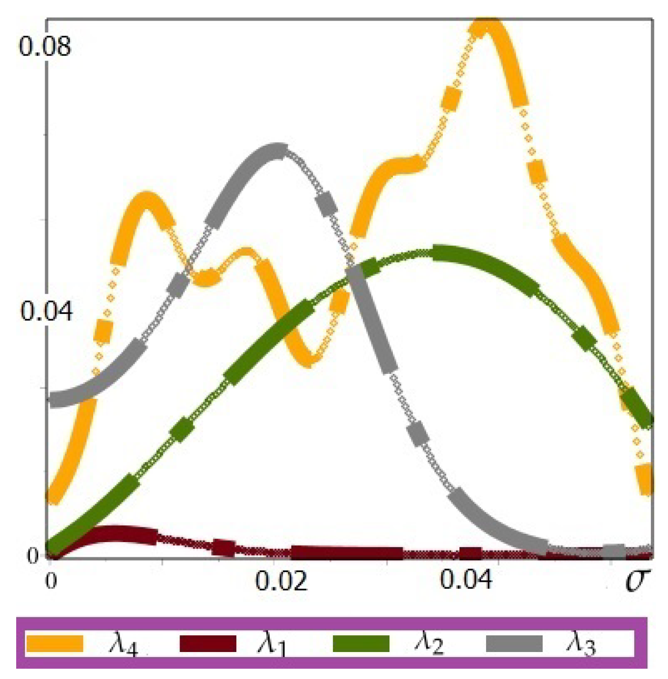
Example 1.

Employing the values provided in [17,18], we consider

$$\left\{\begin{array}{c}\begin{array}{cc}{}^{\mathcal{HH}\mathcal{H}}D_a^{{\displaystyle \frac{i+2}{i+1}},0.50,\ln \left(\sigma \right)}{\varphi }_i\left(\sigma \right)={\displaystyle \frac{1}{3({25}^{\sigma }+5)[1+{\sum }_{j=1}^n|{\varphi }_j\left|\right]}},& \sigma \in \varpi =(a,N],i=1,\cdots ,n,\\ {\varphi }_i\left(a\right)=0,& {\varphi }_i\left(2\right)=3I_{a^{+}}^{0.50,\ln \left(\sigma \right)}{\varphi }_i\left(1.50\right).\end{array}\hfill \end{array}\right.$$

(20)

Here, ${\mathfrak{P}}_{1i}={\displaystyle \frac{i+2}{i+1}},{\mathfrak{P}}_{2i}={\mathfrak{P}}_{3i}=0.50,$ ${\mathfrak{P}}_{0i}={\displaystyle \frac{3i+4}{2i+2}},$ $a=0.01,$$N=1,$ ${\delta }_1=1.50,$ and $({\varphi }_1,\cdots ,{\varphi }_n)\in {\mathbb{R}}_{+}.$ Clearly, ${\mathrm{\Phi }}_i(\sigma ,\varphi )$ are nonnegative and continuous with $|{\mathrm{\Phi }}_i(\sigma ,\varphi )-{\mathrm{\Phi }}_i(\sigma ,\tilde{\varphi })|\le {\displaystyle \frac{1}{90}}{\sum }_{r=1}^n|{\varphi }_r-{\tilde{\varphi }}_r|,$ for every $({\varphi }_1,\cdots ,{\varphi }_n),({\tilde{\varphi }}_1,\cdots ,{\tilde{\varphi }}_n)\in {\mathbb{R}}_{+}^n.$

Here, ${\varrho }_i={\displaystyle \frac{1}{90}}.$ For $(\sigma ,{\varphi }_1,\cdots ,{\varphi }_n)\in (a,N]\times {\mathbb{R}}_{+}^n,$ we obtain ${\displaystyle \frac{1}{90}}\le {\mathrm{\Phi }}_i(\sigma ,\varphi )\le {\displaystyle \frac{1}{3}},$ so for Theorem 2, ${\zeta }_{1i}={\displaystyle \frac{1}{90}},$ and ${\zeta }_{2i}={\displaystyle \frac{1}{3}}.$ Thus, the fractional-order system has a positive solution $({\varphi }_{\diamond 1},\cdots ,{\varphi }_{\diamond n})\le ({\varphi }_1,\cdots ,{\varphi }_n)\le ({\varphi }_1^{\diamond },\cdots ,{\varphi }_n^{\diamond }),$ where

$$\begin{array}{ccc}\hfill {\varphi }_i^{\diamond }\left(\sigma \right)& =& {\displaystyle \frac{-1}{3}}{\displaystyle \frac{{\left[\ln \left(\frac{\sigma }{a}\right)\right]}^{\frac{3i+4}{2i+2}-1}}{15}}\left[{\displaystyle \frac{3}{\mathrm{\Gamma }(\frac{i+2}{i+1}+1.50)}}{\left[\ln \left({\displaystyle \frac{1.50}{a}}\right)\right]}^{{\displaystyle \frac{i+2}{i+1}}+0.50}-{\displaystyle \frac{1}{\mathrm{\Gamma }(\frac{i+2}{i+1}+1)}}{\left[\ln \left({\displaystyle \frac{N}{a}}\right)\right]}^{{\displaystyle \frac{i+2}{i+1}}}\right]\hfill \\ & & +{\displaystyle \frac{1}{3\mathrm{\Gamma }(\frac{i+2}{i+1}+1)}}{\left[\ln \left({\displaystyle \frac{\sigma }{a}}\right)\right]}^{{\displaystyle \frac{i+2}{i+1}}},\hfill \end{array}$$

and

$$\begin{array}{ccc}\hfill {\varphi }_{i\diamond }\left(\sigma \right)& =& {\displaystyle \frac{1}{90}}{\displaystyle \frac{{\left[\ln \left(\frac{\sigma }{a}\right)\right]}^{\frac{3i+4}{2i+2}-1}}{{\eta }_i}}\left[{\displaystyle \frac{3}{\mathrm{\Gamma }(\frac{i+2}{i+1}+1.50)}}{\left[\ln \left({\displaystyle \frac{1.50}{a}}\right)\right]}^{{\displaystyle \frac{i+2}{i+1}}+0.50}-{\displaystyle \frac{1}{\mathrm{\Gamma }(\frac{i+2}{i+1}+1)}}{\left[\ln \left({\displaystyle \frac{N}{a}}\right)\right]}^{{\displaystyle \frac{i+2}{i+1}}}\right]\hfill \\ & & +{\displaystyle \frac{1}{90\mathrm{\Gamma }(\frac{i+2}{i+1}+1)}}{\left[\ln \left({\displaystyle \frac{\sigma }{a}}\right)\right]}^{{\displaystyle \frac{i+2}{i+1}}},\hfill \end{array}$$

for $i=1,\cdots ,n$ and ${\eta }_i={\left[\ln \left({\displaystyle \frac{N}{a}}\right)\right]}^{{\displaystyle \frac{3i+4}{2i+2}}-1}-3I_a^{0.50,\ln \left(\sigma \right)}{\left[\ln \left({\displaystyle \frac{1.50}{a}}\right)\right]}^{{\displaystyle \frac{3i+4}{2i+2}}-1}.$ Set $n=4.$ We have $\tau =\max \{{\tau }_1,\cdots ,{\tau }_4\}\approx 0.55.$ Hence, the conditions of Theorem 2 are satisfied. Thus, (20) has a unique positive solution on $(a,b).$ For $\mathrm{\Theta }=\max \{{\mathrm{\Theta }}_1,\cdots ,{\mathrm{\Theta }}_4\},$ we consider

$$|{}^{\mathcal{HH}}D_a^{{\displaystyle \frac{i+2}{i+1}},0.50,\ln \left(\sigma \right)}{\tilde{\varphi }}_i\left(\sigma \right)-{\displaystyle \frac{1}{3({25}^{\sigma }+5)[1+{\sum }_{j=1}^n|{\tilde{\varphi }}_j\left|\right]}}|\le \mathrm{\Theta }{\mathfrak{G}}_2{\phi }_i.$$

Thus, (20) is stable of the second type with $\parallel ({\tilde{\varphi }}_1,\cdots ,{\tilde{\varphi }}_4)-({\varphi }_1,\cdots ,{\varphi }_4){\parallel }_{2-{\mathfrak{P}}_0,\ln \left(\sigma \right)}\le \mathrm{\Theta }{\mathfrak{G}}_2\phi ,$ where ${\mathfrak{G}}_2={\displaystyle \frac{1}{\mathcal{L}}}{\sum }_{j=1}^4{\sum }_{i=1}^4{\beta }_{ji}\mathcal{D},$ and

$$\begin{array}{c}\hfill \mathcal{D}=\underset{i=1,\cdots ,4}{\max }\left[{\displaystyle \frac{\ln \left(\frac{\sigma }{a}\right)}{{\eta }_i}}\left({\displaystyle \frac{3{\left[\ln \left(\frac{1.50}{a}\right)\right]}^{\frac{i+2}{i+1}+0.50}}{\mathrm{\Gamma }(\frac{i+2}{i+1}+1.50)}}-{\displaystyle \frac{{\left[\ln \left(\frac{N}{a}\right)\right]}^{\frac{i+2}{i+1}}}{\mathrm{\Gamma }(\frac{i+2}{i+1}+1)}}\right)+{\displaystyle \frac{{\left[\ln \left(\frac{\sigma }{a}\right)\right]}^{\frac{i+2}{i+1}}}{\mathrm{\Gamma }(\frac{i+2}{i+1}+1)}}\right].\end{array}$$

Here, we set the control functions $\underset{\underset{i=1,\cdots ,4}{︸}}{{\phi }_i}$ as the hypergeometric function (HF), the Mittag–Leffler function (MLF), the Wright function (WF), and the exponential function (EF), respectively. The obtained errors ${\lambda }_i:={\mathrm{\Theta }}_i{\mathfrak{G}}_2{\phi }_i,i=1,\cdots ,4$ are given in Figure 1. As you can observe, the control function ${\phi }_1$ presents a better estimation of a unique solution with respect to the others.

The obtained errors

$$E_i:={\mathit{argmin}}_{\sigma }\left\{\parallel ({\tilde{\varphi }}_1,\cdots ,{\tilde{\varphi }}_4)-({\varphi }_1,\cdots ,{\varphi }_4){\parallel }_{2-{\mathfrak{P}}_0,\ln \left(\sigma \right)}-\mathrm{\Theta }{\mathfrak{G}}_2{\phi }_i\right\},$$

for $i=1,2,3,4,$ are given in

Table 1. The obtained errors $E_i$ for $i=1,2,3,4.$.

		${\mathit{\sigma }}_1\in$(0.025, 0.050)				${\mathit{\sigma }}_2\in (0.050,0.075)$
		Obtained Errors
${\mathfrak{P}}_{1i}$	${\mathfrak{P}}_{2i}$	$E1$	$E2$	$E3$	$E4$	$E1$	$E2$	$E3$	$E4$
	0.10	0.327	0.465	0.791	0.850	0.515	0.718	0.783	0.876
0.25	0.20	0.361	0.497	0.805	0.871	0.530	0.729	0.797	0.894
	0.30	0.402	0.512	0.830	0.892	0.549	0.740	0.812	0.911
0.50	0.40	0.436	0.530	0.851	0.901	0.568	0.763	0.833	0.937

. The gained errors $E_i,i=1,\cdots ,4,$ for different values of ${\mathfrak{P}}_{1i}$ and ${\mathfrak{P}}_{2i}$ in two different ranges ${\sigma }_1$ and ${\sigma }_2$ indicate that the presence of various special functions as control functions can be effective in optimizing the resulting errors. As mentioned earlier, it can be observed that the control function ${\phi }_1$ plays a more significant role in minimizing the errors.

The primary objective of this example is to introduce a novel concept of Ulam-type stability [17], termed optimal stability, utilizing classical and well-established special functions. This form of stability enables us to achieve various approximations based on the specific special functions selected initially, allowing for the assessment of both maximal stability and minimal error. Research on stability analysis, particularly in the context of Ulam and its various forms, has garnered significant interest among scholars. Nonetheless, effectively generalizing Ulam stability problems and addressing optimized controllability and stability remain pressing challenges. The concept of optimal stability not only encompasses previous theories but also emphasizes the optimization aspect of the problem, facilitating an in-depth exploration of enhancing different types of Ulam stabilities in mathematical models employed within natural sciences and engineering fields.

4. Conclusions and Future Works

This study successfully establishes sufficient conditions for the existence, uniqueness, and optimal stability of positive solutions within the framework of Hilfer–Hadamard fractional differential equations. In employing advanced mathematical tools such as the Mittag–Leffler, Wright, and hypergeometric functions and leveraging fixed point theorems along with nonlinear functional analysis techniques, the theoretical results are comprehensively validated through a pertinent example. This not only reinforces the robustness of the proposed methodology but also highlights its practical applicability in solving real-world problems governed by fractional dynamics. Despite the promising outcomes, there remain numerous avenues for further exploration. Future studies could delve into the extension of these sufficient conditions to larger systems or alternative fractional operators, providing a broader scope of applications. Investigating numerical methods for effectively solving Hilfer–Hadamard fractional differential equations could also enhance the usability of these theoretical findings in computational science and engineering. Furthermore, exploring the influence of varied boundary conditions and external parameters on stability characteristics could yield valuable insights into the behavior of fractional systems in diverse contexts. The results achieved in this paper serve as a foundational step, paving the way for ongoing advancements in fractional calculus and its applications. These efforts will undoubtedly deepen the understanding of fractional differential equations and inspire innovative approaches to tackling complex phenomena across scientific disciplines.