Abstract
The Nikiforov–Uvarov functional analysis (NUFA) formalism is employed to study approximately the eigensolutions of the Schrodinger equation with the Pöschl–Teller-like pseudo-harmonic oscillator (PTPO). The variations in the energy spectra and the wave functions as a function of the screening parameters for different quantum states were investigated. With the energy expression of PTPO, the partition function and other thermodynamic function were obtained as a function of temperature for different values of the screening parameters using the Euler–Maclaurin formula. Using the Hellmann–Feynman theorem (HFT), we evaluate the expectation values of PTPO numerically and graphically for various values of the screening parameters and quantum states. It is observed that the eigensolutions, thermodynamic functions and expectation values of PTPO system are influenced by quantum states, screening parameters and temperature.
Keywords:
eigensolution; pseudo-harmonic oscillator; partition function; entropy; expectation values MSC:
80A05; 81S05; 82B30; 82D40
1. Introduction
For many decades now, different wave equations have been studied to obtain the necessary information concerning any quantum system, with the help of a potential energy function.
One such potential energy function used in physics in modelling diatomic molecules is the Pöschl–Teller potential [1,2,3,4]. Apart from its applications in diatomic molecules, Pöschl–Teller potential plays a vital role in different areas of study including Bose–Einstein condensate, quantum wells, and many body problems, among others [5,6,7,8]. Pöschl–Teller potentials appear in various forms either as circular-like potential or as hyperbolic-like potential.
Many authors have obtained the solutions of Dirac, Klein–Gordon and Schrodinger equations with various forms of Pöschl–Teller potential [9,10,11,12,13,14,15,16]. Recently, the generalized hyperbolic potential model was studied in higher dimensions, using functional analysis method [17]. Considering equal scalar and vector potentials, relativistic and nonrelativistic energies were obtained for selected diatomic molecules. The results obtained for selected diatomic molecules exhibit inter-dimensional degeneracy symmetry. Also, analytical solution of Bohr Hamilton with trigonometric Pöschl–Teller potential with stable and unstable nuclei pictures was obtained using asymptotic iteration method (AIM) [18]. Here, transition rates were computed, and their results agree with experimental data. Eyube and he co-authors [19] studied the improved Pöschl–Teller oscillator using improved quantization rule. Analytical expression for the bound state energies and thermodynamic functions for the oscillator were considered for the RbH diatomic molecule. In another development, Omugbe and his collaborators [20] considered a mixed hyperbolic Pöschl–Teller potential in hyper-radial space using WKB approximation and parametric NU methods. In their studies, thermodynamic properties and mean values were obtained for varying quantum states arbitrarily. Recently, the effect of global monopole on trigonometric Pöschl–Teller potential was studied [21]. Here, the global monopole causes modification in the eigensolutions of the quantum particles studied. Also, approximate solutions of the Dirac equation with spin and pseudospin symmetries were obtained for q-deformed hyperbolic potential containing a Coulomb-like tensor interaction. The ro-vibrational energies obtained for some diatomic molecules were consistent with RKR data in the literature [22].
In our study, we consider the Pöschl–Teller-like pseudo-harmonic oscillator (PTPO) of the form:
Here, are potential constants and is the screening parameter.
In this work, we derive the energy expression of the PTPO and its normalized wave function, using NUFA method [23]. The NUFA method is employed in this work due to its effectiveness and simplicity in usage, as compared to other analytical methods. The partition function expression and other thermodynamic properties expressions for the PTPO are obtained using the Euler–Maclaurin formula [24,25,26]. The expectation values of the PTPO, using the Hellmann–Feynman theorem (HFT) [27,28,29,30,31] are obtained in a closed form. The numerical solutions of the energies and expectation values for the PTPO at varying screening parameters and quantum states are analyzed. The graphical variations in the expectation values, wave functions and thermodynamic functions with quantum states, radial distance and temperature, respectively, at various screening parameters are illustrated.
This paper is organized as follows. The bound state solution and the normalized wave function for the PTPO are given in Section 2. The thermodynamic functions of PTPO are obtained in Section 3. In Section 4, the expectation values expressions are presented for the PTPO. Section 5 presents the numerical and graphical results obtained and their subsequent discussions. Section 6 gives the concluding remarks.
2. Bound State Solutions of the PTPO
The Schrödinger equation (SE) in three dimensions reads [32],
where represents the reduced Planck constant, reduced mass, the potential interaction, the energy and the wave function, respectively. By using the ansatz together with Equation (1), then the radial SE from Equation (2) becomes
It has been established in the literature that Equation (3) does not have analytical solutions because of the centrifugal barrier except for the s-wave corresponding to . To find the analytical solution of Equation (3), we adopt the following approximation scheme [33,34],
Here, the dimensionless parameters are . It is worth mentioning that the approximation given in Equation (4) is adopted due to the fact that it gives improved results for the long-range screening parameter, as compared to the Greene–Aldrich approximation , which is appropriate for small values of the screening parameter [20].
Substituting Equation (4) into Equation (3) gives,
In view of the new coordinate transformation, leads Equation (5) into the form,
where
In order to obtain the bound state solution, one can see that as when and when . Thus, the wave function takes the form,
Substituting Equation (8) into Equation (6) and using NUFA method (see Appendix A), we obtain and as,
The energy spectrum is obtained using Equation (A15) as,
Let us now make a special remark on the energy spectrum of Equation (11). The PTPO of Equation (1) reduced to the well-known pseudo-harmonic potential if we map , as . Thus, the energy spectrum for the pseudo-harmonic potential becomes,
Equation (12) reduces to the standard harmonic oscillator when .
The corresponding wave function is determined using Equation (A16) as,
where is the normalization constant and the constants are defined as follows:
In terms of Jacobi polynomials, we have
where
To obtain the normalization constant, the normalization condition of the radial wave function is employed:
Hence,
Here,
By using the transformation , we have
By using the symmetry relation of the Jacobi polynomials, we have [35]
Hence, Equation (22) becomes,
From the standard integral formula [35],
By comparing Equation (24) and Equation (25), the normalization constant becomes
The total wave function for the PTPO now becomes,
3. Thermodynamic Functions for the PTPO
The determination of partition function is the beginning point of consideration of the thermodynamic properties [36,37]. For any system under consideration, the partition function is given as:
Here, the energy eigenvalue expression of Equation (11) is re-written as
where
The upper vibration quantum number is obtained using the expression .
Hence, .
We employ the Euler–Maclaurin formula defines as [24,25,26]
where are the Bernuoli numbers, is the derivative of order . Taking up to , we obtain
where , and .
With the help of the Mathematica software 13.3 and the Euler–Maclaurin formula, the expression for the partition function of the Pöschl–Teller-like pseudo-harmonic oscillator is obtained as
where
Other thermodynamic properties such as Helmholtz free energy, , entropy, , internal energy, , and specific heat capacity, can be obtained from the partition function as follows [38]:
4. Expectation Values of the PTPO
Generally, the Hellmann–Feynman theorem (HFT) is used to evaluate the expectation values of some quantum observables for any quantum numbers n and [27]. The HFT is related to the derivative of the total energy eigenvalues with respect to any parameter q and the expectation value of the Hamiltonian with respect to that same parameter [39]. The HFT is defined as follows:
Provided the normalized wave function is continuous with respect to the parameter . The effective Hamiltonian for the Pöschl–Teller-like pseudo-harmonic oscillator is given as
By setting in Equation (36) and using Equations (11) and (37), the expectation values of are obtained as
By setting in Equation (36) and using Equations (11) and (37), the expectation values of are obtained as
By setting in Equation (36) and using Equations (11) and (37), the expectation values of are obtained using the relation:
Hence,
By setting in Equation (36) and using Equations (11) and (37), the expectation values of are obtained using the relation:
Hence,
where .
5. Results and Discussion
In this study, we solved the radial Schrödinger equation in three dimensions with the PTPO, using the NUFA formalism. The closed form energy spectrum is presented in Equation (11). The energy spectrum of the pseudo-harmonic potential obtained as a special case is presented in Equation (12). Also, the corresponding normalized wave function of the PTPO is obtained from Equation (27). The following arbitrary parameters are used throughout our computations: . Also, the unit of the energy calculated is in fermi per metre . Table 1 shows the energies of the PTPO at different quantum states for various screening parameters. At a particular quantum state, the energy decreases with an increase in screening parameters. Also, for each screening parameter, the energies are seen to decrease with an increase in the quantum state considered. This shows that the energy levels of PTPO are greatly influenced by screening parameter and quantum states.

Table 1.
Bound state energy eigenvalues of the Pöschl–Teller-like pseudo-harmonic oscillator at different quantum states for various screening parameters.
In addition, plots of the normalized wave function and probability density at different states and principal quantum numbers are presented for various screening parameters. In Figure 1a, the variations in the ground state wave function of PTPO with internuclear distance are presented. Here, equally distanced wave curves are seen with their peaks inversely proportional to the screening parameter values. In Figure 1b, its probability density curves presented are seen to be the same, just that more electron density are concentrated at higher screening parameter values. Figure 2 and Figure 3 show the variation in the first excited and second excited states of PTPO with internuclear distance, respectively, with internuclear distance, and their corresponding probability densities. Both the first excited and second excited wave functions in Figure 2a,b show periodic and sinusoidal curves with increased peaks corresponding to the quantum number. Also, the probability densities shown in Figure 2b and Figure 3b, respectively, show an increase in their peaks, as compared to Figure 2a and Figure 3a. In Figure 4, variations in normalized wave function of PTPO with internuclear distance and its probability density plot are presented for varying quantum numbers. Sinusoidal wave curves are observed in both cases. It can be confirmed here that the peak of the curves increases as the quantum number increases. This is in line with the theoretical and experimental description of probability density [40].
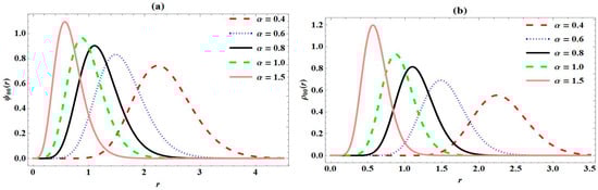
Figure 1.
Variation in (a) ground state wave function of Pöschl–Teller-like pseudo-harmonic oscillator with radial distance; (b) ground state probability density of Pöschl–Teller-like pseudo-harmonic oscillator with radial distance; for various screening parameters.
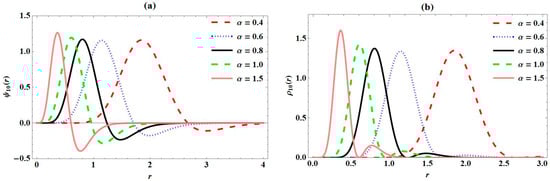
Figure 2.
Variation in (a) first excited state wave function of Pöschl–Teller-like pseudo-harmonic oscillator with radial distance; (b) first excited state probability density of Pöschl–Teller-like pseudo-harmonic oscillator with radial distance; for various screening parameters.
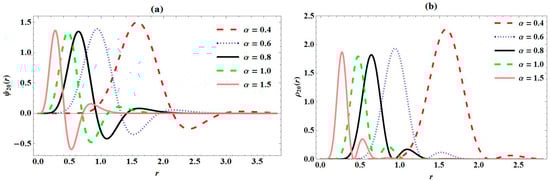
Figure 3.
Variation in (a) second excited state wave function of Pöschl–Teller-like pseudo-harmonic oscillator with radial distance; (b) second excited state probability density of Pöschl–Teller-like pseudo-harmonic oscillator with radial distance; for various screening parameters.
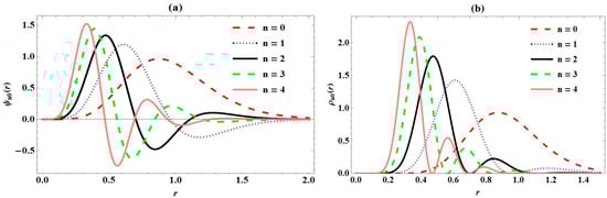
Figure 4.
Variation in (a) wave function of Pöschl–Teller-like pseudo-harmonic oscillator with radial distance; (b) probability density of Pöschl–Teller-like pseudo-harmonic oscillator with radial distance; for various principal quantum numbers .
The closed form expressions of partition function and other thermodynamic functions of PTPO are presented in Equations (33) and (35), respectively. In Figure 5, the variations in these thermodynamic functions with temperature are presented for varying screening parameter values. The partition function decreases with an increase in temperature, as seen in Figure 5a. Also, the partition function n curves increase with increase in screening parameter values considered, at a unique temperature value. These behaviours are also observed in Figure 5c,d for internal energy and entropy, respectively. But, in Figure 5c,d, the curves tend to converge as the temperature is enhanced more. The free energy curves in Figure 5b decrease first and later increase, as the temperature is enhanced. In addition, the free energy curves decrease with increase in screening parameter, at any temperature value considered. In Figure 5e, the specific heat capacity curves rise abruptly at a specific temperature value. As the temperature increases, the curves decrease gradually and later converge at higher temperature values. At this point, the specific heat capacity values are reduced with increase in screening parameter values considered. It is evidentially here that the specific heat capacity curves of PTPO produce unique critical values of temperature, corresponding to each screening parameter values considered. This phenomenon agrees with other studies in the literature [41,42,43,44,45].
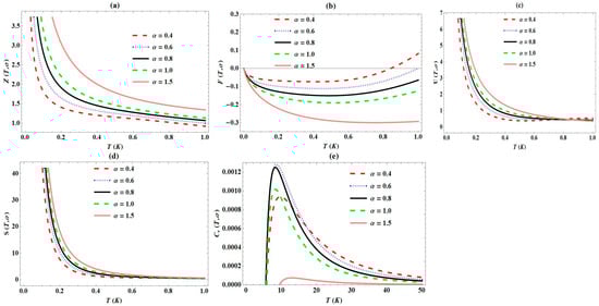
Figure 5.
Variation in (a) partition function; (b) free energy; (c) internal energy; (d) entropy; (e) specific heat capacity of Pöschl–Teller-like pseudo-harmonic oscillator with temperature for various screening parameters.
Different expressions of the expectation values are obtained in closed forms using the HFT, as presented in Equations (38), (39), (41) and (43), respectively, for , , and . Their numerical results are presented in Table 2, Table 3, Table 4, Table 5 and Table 6. In Table 2, the expectation values of decrease with increases in quantum states and screening parameters. The expectation values of decrease as the screening parameters increase for a particular quantum state, as shown in Table 3. Also, there is a corresponding increase in the expectation values of as the quantum states increase, considering a unique screening parameter. In Table 4, the expectation values of momentum squared () increases with increase in screening parameter, for any quantum state. In addition, a decrease in expectation values of is observed when the quantum state increases. Further increase in the quantum state causes the expectation values of to decrease for any screening parameter considered. In Table 5, the expectation values of the inverse squared position space () decrease with an increase in screening parameter for any quantum state. It also decreases with an increase in quantum states for a particular screening parameter. We obtained the numerical product of the expectation values of and , as shown in Table 6. Here, the combined expectation values decrease with an increase in quantum states and the screening parameters considered.
Table 2.
Expectation values of for Pöschl–Teller-like pseudo-harmonic oscillator at various quantum states and screening parameters.
Table 3.
Expectation values of for Pöschl–Teller-like pseudo-harmonic oscillator at various quantum states and screening parameters.
Table 4.
Expectation values of for Pöschl–Teller-like pseudo-harmonic oscillator at various quantum states and screening parameters.
Table 5.
Expectation values of for Pöschl–Teller-like pseudo-harmonic oscillator at various quantum states and screening parameters.
Table 6.
Expectation values of for Pöschl–Teller-like pseudo-harmonic oscillator at various quantum states and screening parameters.
To justify these numerical results of expectation values, Figure 6, Figure 7, Figure 8, Figure 9 and Figure 10 show variation in different expectation values of PTPO with quantum numbers for varying screening parameters considered. In Figure 6a, we observe a sharp decrease in plots with an increase in principal quantum number , for all values of the screening parameter . Also, the expectation values of decrease with increase in for any value of . We observed a unique increase in plots for negative values of orbital angular momentum quantum number in Figure 6b, for . Also, there exist a convergence of these curves around . As increases, plots decrease uniquely. For , we observe a direct decrease in plots as increases. Figure 7a depicts the same behaviour as that of Figure 6a, for expectation values plots of with , for all values of . We observe in Figure 7b that there exists a decrease in plots for , and thereafter an increase in plots for positive values of , as regards . For , we observe a direct decrease in plots with increases in . In Figure 8a, the expectation value plots of increase directly as increases. For a particular value of , these plots increase with increase in values considered. In Figure 8b, we observe a sharp decrease in the expectation value plots of to a specific value, corresponding to unique negative values of for . Thereafter, the expectation value curves of converge together for values of closer to the origin. As is enhanced beyond the origin positively, the plots of increase sharply at unique values of . For , the expectation value plots increase directly as increases. The trend of plots for expectation values of seen in Figure 9a are the same as those observed in Figure 6a and Figure 7a. In Figure 9b, we observe the same trend as that observed in Figure 8b for , where the convergence of the curves is at the origin. Also, the curves decrease directly as increases, for . We also plot the product of the expectation values of and in Figure 10. In Figure 10a, we observe a monotonous decrease in the combined curves for increasing . Also, the combined curves decrease with increases in , for every considered. For , the combined curves first increase sharply at unique values of negative and then converge at values closer to origin, as seen in Figure 10b. As increases positively, there exists a sharp decrease in the combined curves at unique values of . For , we observe a monotonous increase and decrease in the combined curves, as increases.
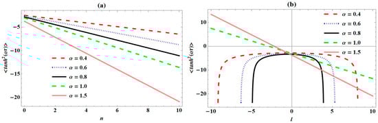
Figure 6.
Variation in expectation values of with (a) principal quantum number (n); (b) angular momentum quantum number (l) for Pöschl–Teller-like pseudo-harmonic oscillator with quantum numbers for various screening parameters.
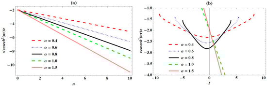
Figure 7.
Variation in expectation values of with (a) principal quantum number (n); (b) angular momentum quantum number (l) for Pöschl–Teller-like pseudo-harmonic oscillator with quantum numbers for various screening parameters.
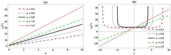
Figure 8.
Variation in expectation values of with (a) principal quantum number (n); (b) angular momentum quantum number (l) for Pöschl–Teller-like pseudo-harmonic oscillator with quantum numbers for various screening parameters.
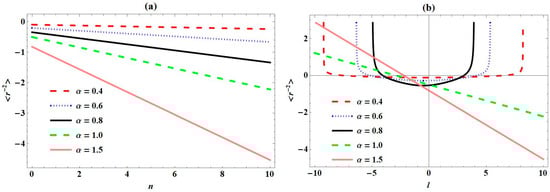
Figure 9.
Variation in expectation values of with (a) principal quantum number (n); (b) angular momentum quantum number (l) for Pöschl–Teller-like pseudo-harmonic oscillator with quantum numbers for various screening parameters.
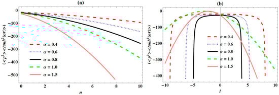
Figure 10.
Variation in expectation values of with (a) principal quantum number (n); (b) angular momentum quantum number (l) for Pöschl–Teller-like pseudo-harmonic oscillator with quantum numbers for various screening parameters.
6. Concluding Remarks
In this work, we have employed the NUFA method to derive the energy expression of PTPO and its normalized wave function in closed form. With the help of the energy expression, we obtained the partition function and other thermodynamic functions expressions using the Euler–MacLaurin formula. In addition, we employed the HFT to derive the expectation value expressions for the PTPO. Variation in numerical results of energy with quantum numbers has been presented for varying screening parameters. Energy variation is seen to decrease with an increase in screening parameters, at unique quantum states. In addition, the energy is observed to decrease with an increase in the quantum state for each screening parameter considered. This shows that the energy eigenstates are influenced by the screening parameters and quantum numbers.
The wave functions and probability densities at various states have been considered with various screening parameters. Different periodic and sinusoidal curves have been obtained, with their peaks corresponding to the quantum numbers considered. Here, distanced wave curves at their peaks are observed to be inversely proportional to the screening parameter values. Also, the peaks of these curves are seen to increase with an increase in quantum numbers.
The thermodynamic plots were obtained with respect to temperature. Specific results obtained here are that the specific heat capacity curves of PTPO produce unique critical values of temperature, corresponding to each screening parameter value considered. These results show excellent agreement with results in the literature, especially at unique critical temperatures [46,47].
We have extended our studies to the variation in different expectation values with quantum numbers for varying screening parameters. The expectation values of the proposed potential model reveal the variable average phenomena of the properties considered, with respect to the quantum numbers and screening parameters considered.
We intend to extend this work to the relativistic regime, with the effect of some topological defects.
Author Contributions
Conceptualization, H.I.A. and A.N.I.; Methodology, U.S.O.; Software, U.S.O. and R.H.; Validation, R.H. and A.N.I.; Formal Analysis, H.I.A. and U.S.O.; Investigation, R.H. and A.N.I.; Supervision, A.N.I. and G.J.R.; Project management, H.I.A. and G.J.R.; Writing—review and edition, H.I.A., U.S.O. and A.N.I. All authors have read and agreed to the published version of the manuscript.
Funding
The work was funded by Princess Nourah bint Abdulrahman University Researchers Supporting Project number (PNURSP2025R106), Princess Nourah bint Abdulrahman University, Riyadh, Saudi Arabia.
Data Availability Statement
The original contributions presented in this study are included in the article. Further inquiries can be directed to the corresponding author.
Acknowledgments
U.S. Okorie thanks the University of South Africa for the Postdoctoral Fellowship position in the Department of Physics, College of Science, Engineering and Technology.
Conflicts of Interest
The authors declare no conflict of interest.
Appendix A
Review of Nikiforov–Uvarov Functional Analysis (NUFA) Method
Using the concepts of NU method [48], parametric NU method [49] and the functional analysis method [50], we proposed a simple and elegant method for solving a second order differential equation of the hypergeometric type called Nikiforov–Uvarov-Functional Analysis (NUFA) method. As it is well-known, the NU is used to solve a second-order differential equation of the form [51]
where and are polynomials, at most of second degree, and is a first-degree polynomial. Tezcan and Sever [49] latter introduced the parametric form of NU method in the form,
where and are all parameters. It can be observed in Equation (A2) that the differential equation has two singularities at and ; thus, we take the wave function in the form,
Substituting Equation (A3) into Equation (A2) leads to the following equation,
Equation (A4) can be reduced to a Gauss hypergeometric equation if and only if the following functions vanish,
Thus, Equation (A4) now becomes,
Solving Equations (A5) and (A6) completely give,
Equation (A7) is the hypergeometric equation type of the form,
where are given as follows,
Setting either or equal to a negative integer , the hypergeometric function turns to a polynomial of degree . Hence, the hypergeometric function approaches finite in the following quantum condition, i.e., , where .
Using the above quantum condition,
Squaring both sides of Equation (A14) and rearranging, we obtain the energy equation for the NUFA method as
By substituting Equations (A8) and (A9) into Equation (A3), we obtain the corresponding wave equation for the NUFA method as
where is the normalization constant.
References
- Gertrud, P.; Teller, E. Bemerkungen zur Quantenmechanik des anharmonischen Oszillators. Z. Für Physik 1933, 83, 143–151. [Google Scholar]
- Zhang, M.C.; Wang, Z.B. Bound states of the Klein-Gordon equation and Dirac equation with the Manning-Rosen scalar and vector potentials. Acta Phys Sin. 2006, 55, 0525. [Google Scholar] [CrossRef]
- Liu, X.Y.; Wei, G.F.; Cao, X.W.; Bai, H.G. Spin symmetry for Dirac equation with the trigonometric Pöschl-Teller potential. Int. J. Theor. Phys. 2010, 49, 343–348. [Google Scholar] [CrossRef]
- Hamzavi, M.; Rajabi, A.A. Exact S-wave solution of the trigonometric pöschl-teller potential. Int. J. Quantum Chem. 2012, 112, 1592–1597. [Google Scholar] [CrossRef]
- Saregar, A.; Suparmi, A.; Cari, C.; Yuliani, H. Analysis of Energy Spectra and Wave Function of Trigonometric Poschl-Teller plus Rosen-Morse Non-Central Potential Using Supersymmetric Quantum Mechanics Approach. Res. Inven. Int. J. Eng. Sci. 2013, 2, 14–26. [Google Scholar]
- Vélez, M.; Sicard, A.; Ospina, J. Pöschl-Teller potentials based solution to Hilbert’s tenth problem. Ingeníeria Y Cienc. 2006, 2, 43–57. [Google Scholar]
- Chen, C.Y.; You, Y.; Lu, F.L.; Dong, S.H. The position–momentum uncertainty relations for a Pöschl–Teller type potential and its squeezed phenomena. Phys. Lett. A 2013, 377, 1070–1075. [Google Scholar] [CrossRef]
- Yahya, W.Y.; Oyewumi, K.J.; Assoc, J. Arab Univ. Basic Appl. Sci. 2016, 21, 53. [Google Scholar]
- Büyükiliç, F.; Egˇrifes, H.; Demirhan, D. Solution of the Schrödinger equation for two different molecular potentials by the Nikiforov-Uvarov method. Theor. Chem. Acc. 1998, 98, 192–196. [Google Scholar] [CrossRef]
- Arai, A. Exactly solvable supersymmetric quantum mechanics. J. Math. Anal. Appl. 1991, 158, 63–79. [Google Scholar] [CrossRef]
- Yang, Q.B. A Nearly Discrete Method for Acoustic and Elastic Wave Equations in Anisotropic Media. Acta Photonica Sin. 2003, 32, 882. [Google Scholar] [CrossRef]
- Zhao, X.Q.; Jia, C.S.; Yang, Q.B. Bound states of relativistic particles in the generalized symmetrical double-well potential. Phys. Lett. A 2005, 337, 189–196. [Google Scholar] [CrossRef]
- Wei, G.F.; Dong, S.H. Spin symmetry in the relativistic symmetrical well potential including a proper approximation to the spin–orbit coupling term. Phys. Scr. 2010, 81, 035009. [Google Scholar] [CrossRef]
- Wei, G.F.; Dong, S.H. Algebraic approach to pseudospin symmetry for the Dirac equation with scalar and vector modified Pöschl-Teller potentials. Europhys. Lett. 2009, 87, 40004. [Google Scholar] [CrossRef]
- Candemir, N. Klein–Gordon particles in symmetrical well potential. Appl. Math. Comput. 2016, 274, 531–538. [Google Scholar] [CrossRef]
- Durmus, A. Approximate treatment of the Dirac equation with hyperbolic potential function. Few-Body Syst. 2018, 59, 7. [Google Scholar] [CrossRef]
- Okorie, U.S.; Ikot, A.N.; Edet, C.O.; Rampho, G.J.; Sever, R.; Akpan, I.O. Solutions of the Klein Gordon equation with generalized hyperbolic potential in D-dimensions. J. Phys. Commun. 2019, 3, 095015. [Google Scholar] [CrossRef]
- Hammou, A.A.B.; Chabab, M.; El Batoul, A.; Hamzavi, M.; Lahbas, A.; Moumene, I.; Oulne, M. Bohr Hamiltonian with trigonometric Pöschl-Teller potential in-unstable and-stable pictures. Eur. Phys. J. Plus 2019, 134, 577. [Google Scholar] [CrossRef]
- Eyube, E.S.; Bitrus, B.M.; Jabil, Y.Y. Thermodynamic relations and ro-vibrational energy levels of the improved Pöschl–Teller oscillator for diatomic molecules. J. Phys. B At. Mol. Opt. Phys. 2021, 54, 155102. [Google Scholar] [CrossRef]
- Omugbe, E.; Osafile, O.E.; Okon, I.B. Approximate eigensolutions, thermodynamic properties and expectation values of a mixed hyperbolic Pöschl–Teller potential (MHPTP). Eur. Phys. J. Plus 2021, 136, 1–18. [Google Scholar] [CrossRef]
- Ahmed, F.; Bouzenada, A.; Moreira, A.R.P. Global monopole effects on exact s-state solution under trigonometric Pöschl–Teller potential. Mol. Phys. 2024, 123, e2365420. [Google Scholar] [CrossRef]
- Hachama, M.; Diaf, A. Ro-vibrational relativistic states for the q-deformed hyperbolic barrier potential. Eur. Phys. J. Plus 2024, 139, 501. [Google Scholar] [CrossRef]
- Ikot, A.N.; Okorie, U.S.; Amadi, P.O.; Edet, C.O.; Rampho, G.J.; Sever, R. The Nikiforov–Uvarov-Functional Analysis (NUFA) Method: A new approach for solving exponential-type potentials. Few-Body Syst. 2021, 62, 9. [Google Scholar] [CrossRef]
- Boumali, A. The statistical properties of q-deformed Morse potential for some diatomic molecules via Euler–MacLaurin method in one dimension. J. Math. Chem. 2018, 56, 1656–1666. [Google Scholar] [CrossRef]
- Arfken, G. Mathematical Methods for Physicists, 3rd ed.; Academic Press: San Diego, CA, USA, 1985. [Google Scholar]
- Chabi, K.; Boumali, A. Thermal properties of three-dimensional Morse potential for some diatomic molecules via Euler-Maclaurin approximation. Rev. Mex. De Física 2020, 66, 110–120. [Google Scholar] [CrossRef]
- Feynman, R.P. Forces in molecules. Phys. Rev. 1939, 56, 340. [Google Scholar] [CrossRef]
- Bader, R.F.; Jones, G.A. The Hellmann–Feynman theorem and chemical binding. Can. J. Chem. 1961, 39, 1253–1265. [Google Scholar] [CrossRef]
- Okon, I.B.; Popoola, O.; Isonguyo, C.N. Approximate Solutions of Schrodinger Equation with Some Diatomic Molecular Interactions Using Nikiforov-Uvarov Method. Adv. High Energy Phys. 2017, 2017, 9671816. [Google Scholar] [CrossRef]
- Politzer, P.; Murray, J.S. Electronegativity—A perspective. J. Mol. Mod. 2018, 24, 214. [Google Scholar] [CrossRef]
- Okon, I.B.; Onate, C.A.; Omugbe, E.; Okorie, U.S.; Antia, A.D.; Onyeaju, M.C.; Li, C.W.; Araujo, J. Approximate Solutions, Thermal Properties, and Superstatistics Solutions to Schrödinger Equation. Adv. High Energy Phys. 2022, 2022, 5178247. [Google Scholar] [CrossRef]
- Griffiths, D.J.; Schroeter, D.F. Introduction to Quantum Mechanics; Cambridge University Press: Navi Mumbai, India, 2018. [Google Scholar]
- You, Y.; Lu, F.L.; Sun, D.S.; Chen, C.Y.; Dong, S.H. Solutions of the second Pöschl–Teller potential solved by an improved scheme to the centrifugal term. Few-Body Syst. 2013, 54, 2125–2132. [Google Scholar] [CrossRef]
- Ikhdair, S.M.; Falaye, B.J. Approximate analytical solutions to relativistic and nonrelativistic Pöschl–Teller potential with its thermodynamic properties. Chem. Phys. 2013, 421, 84–95. [Google Scholar] [CrossRef]
- Gradstein, I.S.; Ryzhik, I.M. Tables of Integrals, Series, and Products; Jeffrey, A., Zwillinger, D., Eds.; Academic Press: Burlington, MA, USA, 2007. [Google Scholar]
- Khordad, R.; Ghanbari, A. Analytical calculations of thermodynamic functions of lithium dimer using modified Tietz and Badawi-Bessis-Bessis potentials. Comput. Theor. Chem. 2019, 1155, 1–8. [Google Scholar] [CrossRef]
- Jia, C.-S.; You, X.-T.; Liu, J.-Y.; Zhang, L.-H.; Peng, X.-L.; Wang, Y.-T.; Wei, L.-S. Prediction of enthalpy for the gases Cl2, Br2, and gaseous BBr. Chem. Phys. Lett. 2019, 717, 16–20. [Google Scholar] [CrossRef]
- Edet, C.O.; Ikot, A.N. Analysis of the impact of external fields on the energy spectra and thermo-magnetic properties of N2,I2, CO, NO and HCl diatomic molecules. Mol. Phys. 2021, 119, e1957170. [Google Scholar] [CrossRef]
- Oyewumi, K.J.; Sen, K.D. Exact solutions of the Schrödinger equation for the pseudoharmonic potential: An application to some diatomic molecules. J. Math. Chem. 2012, 50, 1039–1059. [Google Scholar] [CrossRef]
- Okon, I.B.; Onate, C.A.; Horchani, R.; Popoola, O.O.; Omugbe, E.; William, E.S.; Okorie, U.S.; Inyang, E.P.; Isonguyo, C.N.; Udoh, M.E.; et al. Thermomagnetic properties and its effects on Fisher entropy with Schioberg plus Manning-Rosen potential (SPMRP) using Nikiforov-Uvarov functional analysis (NUFA) and supersymmetric quantum mechanics (SUSYQM) methods. Sci. Rep. 2023, 13, 8193. [Google Scholar] [CrossRef]
- Osobonye, G.T.; Adekanmbi, M.; Ikot, A.N.; Okorie, U.S.; Rampho, G.J. Thermal properties of anharmonic Eckart potential model using Euler–MacLaurin formula. Pramana 2021, 95, 98. [Google Scholar] [CrossRef]
- Gabriel, T.O.; Okorie, U.S.; Amadi, P.O.; Ikot, A.N. Statistical analysis and information theory of screened Kratzer–Hellmann potential model. Can. J. Phys. 2021, 99, 583–591. [Google Scholar]
- Udoh, M.E.; Amadi, P.O.; Okorie, U.S.; Antia, A.D.; Obagboye, L.F.; Horchani, R.; Sulaiman, N.; Ikot, A.N. Thermal properties and quantum information theory with the shifted Morse potential. Pramana 2022, 96, 222. [Google Scholar] [CrossRef]
- Bang, J.Y.; Berger, M.S. Possible Equilibra of Interacting Dark Energy Models. Phys. Rev. D 2016, 74, 125012. [Google Scholar] [CrossRef]
- Tawfik, A.; Diab, A. Generalized uncertainty principle: Approaches and applications. Int. J. Mod. Phys. D 2014, 23, 1430025. [Google Scholar] [CrossRef]
- Lütfüoğlu, B.C.; Kříž, J. A comparative interpretation of the thermodynamic functions of a relativistic bound state problem proposed with an attractive or a repulsive surface effect. Eur. Phys. J. Plus 2019, 134, 60. [Google Scholar] [CrossRef]
- Kurnia, P.L.; Cari, C.; Suparmi, A.; Harjana, H. Topological effects on relativistic energy spectra of diatomic molecules under the magnetic field with Kratzer potential and thermodynamic-optical properties. Int. J. Theor. Phys. 2023, 62, 246. [Google Scholar]
- Arnold, F.N.; Uvarov, V.B. Special Functions of Mathematical Physics; Birkhäuser: Basel, Switzerland, 1988; Volume 205. [Google Scholar]
- Tezcan, C.; Sever, R. A general approach for the exact solution of the Schrödinger equation. Int. J. Theor. Phys. 2009, 48, 337–350. [Google Scholar] [CrossRef]
- Falaye, B.J.; Oyewumi, K.J.; Ikhdair, S.M.; Hamzavi, M. Eigensolution techniques, their applications and Fisher’s information entropy of the Tietz–Wei diatomic molecular model. Phys. Scr. 2014, 89, 115204. [Google Scholar] [CrossRef]
- Berkdemir, C. Application of the Nikiforov-Uvarov Method in Quantum Mechanics. In Theoretical Concepts of Quantum Mechanics; IntechOpen: Rijeka, Croatia, 2012; p. 225. [Google Scholar]
Disclaimer/Publisher’s Note: The statements, opinions and data contained in all publications are solely those of the individual author(s) and contributor(s) and not of MDPI and/or the editor(s). MDPI and/or the editor(s) disclaim responsibility for any injury to people or property resulting from any ideas, methods, instructions or products referred to in the content. |
© 2025 by the authors. Licensee MDPI, Basel, Switzerland. This article is an open access article distributed under the terms and conditions of the Creative Commons Attribution (CC BY) license (https://creativecommons.org/licenses/by/4.0/).