Numerical Study of Salt Ion Transport in Electromembrane Systems with Ion-Exchange Membranes Having Geometrically Structured Surfaces

Abstract

This article is devoted to numerically modeling the effect of the geometric modification of the surfaces of ion-exchange membranes in electromembrane systems (EMSs) on the salt ion transport using a 2D mathematical model of the transport process in the desalination channel based on boundary value problems for the coupled system of Nernst–Planck–Poisson and Navier–Stokes equations. The main patterns of salt ion transport are established taking into account diffusion, electromigration, forced convection, electroconvection, and the geometric modification of the surface of ion-exchange membranes. It is shown that the geometric modification of the surface of ion-exchange membranes significantly changes both the formation and development of electroconvection. A significant combined effect of electroconvection and geometric modification of the surface of ion-exchange membranes in the desalination channel on the salt ion transport is shown, as well as a complex, nonlinear, and non-stationary interaction of all the main effects of concentration polarization in the desalination channel.

1. Introduction

Desalination is critical to providing access to clean water in water-stressed regions, especially in the face of population growth and climate change. Research shows that technologies such as reverse osmosis, solar desalination, etc., are becoming more efficient and cost-effective, but there are challenges associated with energy consumption and environmental impacts, such as the formation of toxic brine [1,2,3,4,5,6].

According to article [1], desalination, especially using reverse osmosis, has become a key solution for coastal regions with limited freshwater resources. The authors highlight that the cost of desalination has decreased by 50% over the past two decades, making it more affordable, but energy consumption and the formation of toxic brine remain significant drawbacks. Article [1] discusses the potential reduction in energy consumption by modern seawater desalination technologies (reverse osmosis and electrodialysis) and their limitations, the potential role of advanced materials and innovative technologies in improving performance, and the environmental friendliness of desalination.

Article [2] provides an overview of the challenges and opportunities for obtaining clean water based on solar desalination using photothermal materials. The study describes the problem of salt accumulation, which is currently the main obstacle to the stable operation of solar evaporators.

The article in Frontiers [3] shows that desalination can support ecosystems if carbon dioxide emissions are minimized and brine is managed. However, the authors emphasize the need to monitor the impact on marine ecosystems, which requires further research.

It is known that membrane separation methods for water purification and desalination are increasingly used to solve global problems related to water shortage and aquatic pollution. However, progress in the field of membranes for water purification is hampered by the inherent limitations of traditional membrane materials. Recent advances in the field of methods for controlling the structure and chemical functionality of polymer films can potentially lead to the emergence of new classes of membranes for water purification. In review [4], the authors first discuss the current state of existing membrane technologies for water purification and desalination, highlight their inherent limitations, and determine the current requirements for next-generation membranes. They also offer promising approaches to modifying the membrane surface, which minimize interphase interactions and increase resistance to contamination.

The most environmentally friendly method of water desalination today is the use of electromembrane systems, in which electroconvection is the main mechanism of overlimit transport. Thus, in study [5], an experimental confirmation of the role of electroconvection in porous media is presented. It is shown that vortex flows significantly increase the rate of salt removal.

Review [6] examines in detail recent studies of electroconvection with an emphasis on quantitative experimental and mathematical modeling and modeling of this phenomenon. Approaches to controlling this phenomenon under standard conditions are also discussed.

We will adhere to the definition of electroconvection given in [7,8]. Namely, by electroconvection we will mean any movement of an electrolyte solution caused by the effect of an external electric field on the solution. This effect is modeled as a body (volume) electric force in the Navier–Stokes equation. The origin and influence of the body electric force can be explained as follows. The fixed charge of the matrix of ion-exchange membranes causes a high concentration of counterions and a low concentration of co-ions in the membrane volume. Due to the continuity of the concentration change, a double electric layer (DEL) is formed at the interface. The effect of the electric field on the spatial charge region (SCR) in the DEL of the solution leads to the movement of ions in this layer. Since the ions are hydrated, i.e., surrounded by a hydration shell, they move with it. We will assume that the solution is a viscous and incompressible liquid. In liquids, viscosity is a manifestation of the cohesion forces between molecules. Therefore, the hydration shell, in turn, is connected with the surrounding water molecules by the forces of molecular adhesion. Thus, part of the water surrounding the hydration shell of ions is also involved in the movement. Since the SCR contains almost exclusively counterions, the volume of water moving with them encounters almost no resistance from the counter-flow of volume carried by the co-ions. Therefore, the effect of the electric field on the SPR leads to the transport of the entire (or almost entire) volume of the solution located in this region (the phenomenon of electro-osmosis). Note the significant difference compared to the volume of an electrically neutral solution, in which there is a counter-flow of water volumes associated with ions. Water molecules, not entering the primary hydration shell, are affected by both cations moving from the anode to the cathode and anions moving in the opposite direction. As a result, relatively free water molecules are not transported at all, and the phenomenon of electro-osmosis in an electrically neutral solution is absent.

Dukhin S.S. [9] distinguishes two types of electro-osmosis. Electro-osmosis of the first type (classical electro-osmosis) occurs as a result of the action of an electric field on the equilibrium DEL, which exists regardless of the presence of an external electric field. A different situation occurs with strong polarization of the ion-exchange membrane by an external electric field. In this case, as Rubinstein I. and Shtilman L. [10] first showed, the size of the SPE significantly exceeds the thickness of the equilibrium DEL and can reach micrometer sizes [11]. Then, electro-osmosis of the second type occurs: the transport of the liquid volume under the action of an external electric field to the expanded SPE, which occurs as a result of the action of the same electric field. It is electro-osmosis of the second kind that is the main mechanism that causes the overlimiting transport of salt counterions through the membrane. A large number of works are devoted to the study of the phenomenon of electroconvection [12,13,14,15,16].

In [16,17], the importance of the problem of intensifying the desalination process is discussed, including through geometric modification of the surface of ion-exchange membranes.

At present, the phenomenon of overlimiting mass transport is being intensively studied. However, many issues remain poorly understood. In particular, it is unclear what effect the geometric modification of the membrane surface and the forced flow of the solution in the desalination channel have on the development of electroconvection [18,19,20,21,22]. This article attempts to advance the understanding of this phenomenon and to quantitatively describe the occurrence and development of electroconvection under conditions of forced convection and geometric modification of the membrane surface.

Modification of the membrane surface (nanostructuring and fractal patterns) allows for to reduce of concentration polarization, increases the area of the active zone, and improves selectivity [23,24]. According to Zabolotsky V.I. et al. [25], the concept of profiled ion-exchange membranes was introduced and implemented in 1971 by Gnusin N.P. et al. [26] to accelerate the electrodialysis process by increasing the available membrane surface area and mass transport.

Later, Nikonenko V.V. et al. [27] compared the performance of the electrodialysis process in stacks with non-conductive spacers, ion-exchange resins, or profiled ion-exchange membranes. They showed that in the case of profiled membranes, the production of drinking water is most efficient, the Sherwood number is up to five times higher than that of electrodialysis with non-conductive spacers.

Zabolotsky V.I. and Nikonenko V.V. used heterogeneous membranes with a specific pattern on the membrane surface, consisting of cones located at the nodes of rhombuses (diamond-shaped distribution).

Vasilyeva V.I. et al. [28] used similar profiling and investigated the mechanisms of selective transport of amino acids through ion-exchange membranes during the dialysis process and found a more than twofold increase in ion flux and separation factor. Loza S.A. et al. [29] confirmed the increased diffusion permeability of such membranes. Melnikov et al. used membranes with such a pattern to extract valuable components from dilute wastewater [30]. Liu J. et al. [31] changed the shape of the pattern from a rhombus to a square and obtained an approximately 35% increase in the power density in microbial reverse-electrodialysis cells.

The study by Wessling M., Stockmeier F. et al. [32] is devoted to the analysis of the direction of rotation and the position of electroconvective vortices using the surface patterning method or geometric and electrical inhomogeneity. Wessling M., Stockmeier F. et al. [32] compared the development of electroconvection on two membranes modified with patterns of different surface charges. They analyzed the increase in the area of electroconvective vortices, the direction of their rotation and structural stability in a steady state, as well as the possibilities of controlling electroconvective vortices by introducing certain structural inhomogeneities of the membrane surface to reduce energy losses in the plateau region and more economical operation in EMS in overlimit modes, significantly increasing their efficiency. Recently, membranes with a fractal structure have been developed that increase the surface area by 300%. The efficiency of salt removal reached 99.5% at low pressure [33].

This paper discusses the most promising type of single-sided profiled membranes, which will significantly intensify mass transport and increase the efficiency of electrodialysis (ED) systems. Possible optimization paths are shown using numerical simulation of such a model. The article considers two 2D models of non-stationary electroconvection during binary electrolyte transport in the desalination channel of the EMS under extreme current conditions based on a boundary value problem for the Nernst–Planck–Poisson and Navier–Stokes equations. The first model considers half of the ED desalination flow channel on a cation-exchange membrane (CEM) with geometrically structural heterogeneity of the surface. The second model is half of the channel with the same volumetric flow rate and concentration, but without structural heterogeneity of the membrane surface. We calculated the theoretical current-voltage characteristic and determined the main patterns of salt ion transport.

2. Mathematical Model of Electroconvection in Potentiodynamic Mode in Half of the Desalination Channel with an Ideally Selective Cation Exchange Membrane (CEM) with Modified Surface

2.1. Physical Statement: Solution Domain

The potentiodynamic regime is modeled, and half of the channel at the CEM (Figure 1) is considered. In the middle of the channel, the conditions of local electroneutrality are assumed to be fulfilled, and the concentrations are known. In addition, the initial velocity is given by half of the Poiseuille parabola [7,8] $V_y(0,x,y)=6V_0{\displaystyle \frac{x}{H}}(1-{\displaystyle \frac{x}{H}}),V_x(t,x,y)=0,x\in [{\displaystyle \frac{1}{2}}H,H]$, where $V_0$ is the average (linear) flow velocity.

2.2. Boundary Value Problem for the System of Navier–Stokes and Nernst–Planck–Poisson Equations

Modeling of the electrolyte solution flow and the ion transport process for a binary electrolyte in the desalination channel EDA is performed simultaneously, using a system of Navier–Stokes and Nernst–Planck–Poisson equations, interconnected by an electric force. However, for convenience, the equations and boundary conditions modeling the solution flows and ion transport are considered separately below.

1. 

Modeling of the solution flow

The solution flowing in the desalination channel is affected by several forces:

(1)

The inertial force caused by the solution movement;

(2)

The friction force caused by the viscosity of the solution;

(3)

The body electric force caused by the effect of the electric field on the space charge region;

(4)

The lifting force arising from the density gradient caused by the concentration gradients (concentration polarization) and temperature (Joule heating, dissociation, and recombination reactions).

In this paper, we will study the influence of only the first three forces (inertia, friction, and electric force) on the solution flow and their interaction. In doing so, we will adhere to the generally accepted approach when the body force $\overrightarrow{f}$ is singled out separately. Under this condition, the flow in a sufficiently wide range of pressure and force changes is adequately described by the Navier–Stokes equations:

$${\displaystyle \frac{\partial \overrightarrow{V}}{\partial t}}+(\overrightarrow{V}\nabla )\overrightarrow{V}=-{\displaystyle \frac{1}{{\rho }_0}}\nabla P+\nu \mathrm{\Delta }\overrightarrow{V}+{\displaystyle \frac{1}{{\rho }_0}}\overrightarrow{f},$$

$$div(\overrightarrow{V})=0,$$

where $\nabla$ is the gradient, $\mathrm{\Delta }$ is the Laplace operator, $\overrightarrow{V}$ is the volumetric flow rate of the electrolyte solution, ${\rho }_0$ is the characteristic density of the solution, $P$ is the pressure, $t$ is the time, $\nu$ is the kinematic viscosity coefficient, and $\overrightarrow{f}$ is the body force density. Below, as stated above, the electrical force is considered a body force.

As bound conditions for the Navier–Stokes equations:

(1)

The conditions of solution adhesion on a solid boundary, namely on the curved surface of the cation-exchange membrane $(x,y)\in \mathrm{\Gamma },t\ge 0$:

$\overrightarrow{V}(x,y,t)=0$ at $(x,y)\in \mathrm{\Gamma },t\ge 0$. In the depth of the solution, the velocity is considered constant and is specified as follows: $V_x({\displaystyle \frac{H}{2}},y,t)=0,V_y({\displaystyle \frac{H}{2}},y,t)={\displaystyle \frac{3}{2}}{V}_0.$

(2)

At the inlet, we will assume the velocity along the Poiseuille parabola.

(3)

Since non-stationary vortices can arise in this problem, the boundary conditions for the velocity at the outlet of the desalination channel can give computational artifacts near the outlet. To solve this problem, we use two different methods.

The first method is to extend the channel and extract data at some distance before the outlet. In this case, we can assume that the flow at the outlet is also Poiseuille.

This method is applicable when electroconvection begins at the inlet to the channel and the vortices die out before reaching the outlet. However, in some cases, this leads to an unacceptable increase in the calculation time. In addition, this method is not applicable in the case where electroconvection begins at the channel outlet.

In the second method, we consider the boundary to be open, and the normal voltage on it is taken to be zero. In this case, vortices can freely flow outside the modeled region. In numerical calculations with such a condition, difficulties arise in finding the initial approximation in the Newton method used to solve a nonlinear system of equations in the finite element method.

(4)

The initial flow at the channel inlet will be assumed to be a Poiseuille flow.

Initial and boundary conditions at corner points may, in some cases, be inconsistent. However, with a numerical solution, this is smoothed out fairly quickly, but they can initiate the emergence and development of electroconvective vortices that have a non-physical, i.e., artifactual, nature. To match the initial and boundary conditions at corner points, a method of smoothing out inhomogeneities was used by introducing an exponential weighting function.

When using the above boundary conditions, the influence of any non-hydrodynamic processes on the flow of the solution occurs only through the electrical force $\overrightarrow{f}$, which is not a potential force.

2. 

Modeling of the solution flow

The ion transport for a binary electrolyte in a desalination channel is adequately described by the system of Nernst–Planck and Poisson equations:

$${\overrightarrow{j}}_i=-{\displaystyle \frac{F}{RT}}{z}_i{D}_i{C}_i\nabla \phi -D_i\nabla C_i+C_i\overrightarrow{V},i=1,2,$$

(1)

$${\displaystyle \frac{\partial C_i}{\partial t}}=-div{\stackrel{\rightharpoonup }{j}}_i,i=1,2,$$

(2)

$${\epsilon }_0\mathrm{\Delta }\phi =-F\left(z_1{C}_1+z_2{C}_2\right),$$

(3)

$$\overrightarrow{I}=F\left(z_1{\overrightarrow{j}}_1+z_2{\overrightarrow{j}}_2\right),$$

(4)

where $C_1,C_2$ are the concentrations of cations and anions in the solution, respectively, $z_1,z_2$ are the charge numbers of cations and anions, $D_1,D_2$ are the diffusion coefficients of cations and anions, respectively, $j_1$, $j_2$ is the fluxes of cations and anions, $\phi$ is the electric field potential, ${\epsilon }_0$ is the permittivity of the electrolyte, $F$ is the Faraday constant, $R$ is the gas constant, and $T$ is the absolute temperature. In this case, $P,$ $\overrightarrow{V},$ $\phi ,$ $C_1,C_2$ are unknown functions depending on time $t$ and coordinates $x,y$.

We will consider the potentiodynamic regime:

$$\phi ({\displaystyle \frac{H}{2}},y,t)=0,\phi (H,y,t)=d_{\phi }\cdot t,t\ge 0,y\in [0,L]$$

Along with this condition, we will also use the following boundary conditions:

(1)

In the middle of the channel $x={\displaystyle \frac{H}{2}},y\in [0,L],t\ge 0$, we will consider the boundary concentrations of anions and cations to be known:

$$C_1(t,{\displaystyle \frac{H}{2}},y)=C_{01}$$

(5)

$$C_2(t,{\displaystyle \frac{H}{2}},y)=C_{02}$$

(6)

(2)

On the surface of the cation-exchange membrane, we will consider the boundary concentration of cations to be known, which is determined by its exchange capacity:

$$C_1(t,x,y)=C_{km},(x,y)\in \mathrm{\Gamma },t\ge 0$$

(7)

and also, we will assume that the cation-exchange membrane is ideally selective, that is, impermeable to anions:

$$\left({\displaystyle \frac{\partial C_2}{\partial x}}+{\displaystyle \frac{F}{RT}}{z}_2{C}_2{\displaystyle \frac{\partial \phi }{\partial x}}\right)\left(t,H,y\right)=0.$$

(3)

At the entrance to the channel, we will consider the ion concentrations to be given. Depending on the objectives of the study, they can be considered to be distributed either constantly or according to another law. If the concentrations at the entrance are not constant, we will consider that their distribution corresponds to the maximum current density and that the condition of electroneutrality is satisfied at the entrance.

We will consider the potential distribution at the entrance to be linear:

$$\phi (t,x,0)=d_{\phi }{\displaystyle \frac{2x-H}{H}}$$

(8)

(4)

At the exit from the region under consideration $y=L,x\in \left[0,H\right],t\ge 0$, we will use the condition for concentration, which determines the ion flow at the exit:

$$\begin{array}{l}-\overrightarrow{n}\cdot {\overrightarrow{j}}_i\left(t,x,L\right)=-V_2\left(t,x,L\right)C_i\left(t,x,L\right)\text{ or}\\ -{\displaystyle \frac{F}{RT}}{z}_i{D}_i{C}_i{\displaystyle \frac{\partial \phi }{\partial y}}-D_i{\displaystyle \frac{\partial C_i}{\partial y}}+C_i{V}_2=V_2\left(t,x,L\right)C_i\left(t,x,L\right),i=1,2\end{array}$$

For the potential, we will use a similar condition, which means that there is no current flow through the exit:

$$-\overrightarrow{n}\cdot \nabla \phi \left(t,x,L\right)=0\mathrm{or}{\displaystyle \frac{\partial \phi \left(t,x,L\right)}{\partial y}}=0.$$

(5)

We will accept the initial conditions at $t=0$, if possible, consistent with the remaining boundary conditions:

$$C_1(0,x,y)=C_2(0,x,y)=C_0$$

(9)

For the function $\phi$, as an initial condition, we can take, for example, a linear function independent of $y$:

$$\phi (0,x,y)=d_{\phi }{\displaystyle \frac{2x-H}{H}}.$$

(10)

The influence of transport processes on the flow of the solution is manifested through the electric force, the density of which is equal to $\overrightarrow{f}={\displaystyle \frac{1}{{\rho }_0}}{\epsilon }_0\mathrm{\Delta }\phi \nabla \phi$.

The system of equations was solved by the weak coupling method: at each time step, the velocity field was first calculated (Navier–Stokes); then, the distribution of concentrations and potential (Nernst–Planck–Poisson) was calculated. The iterations continued until convergence in the residual was achieved (<1 × 10⁻⁵).

3. Results of Numerical Analysis

3.1. Calculation Parameters Used for Numerical Solution

To analyze the transport process, many different finite element calculations were performed with different parameters. The most typical results are given below. The width of the region under consideration is H = 2 mm (channel width 6 mm), channel length L = 4H mm, average linear velocity V₀ = 1 mm/s, initial concentration C₀ varied from 0.01 to 10 mol/m³, and potential scan rate 0.005 V/s. Additionally, the cation diffusion coefficient D₁ = 1.331 × 10⁻⁹ [m²/s], the anion diffusion coefficient D₂ = 2.051 × 10⁻⁹ [m²/s], the cation charge number z₁ = 1, the anion charge number z₂ = −1, $\nu$= 0.89371 × 10⁻³ [Pas] is the kinematic viscosity coefficient, R is the universal gas constant, T is the absolute temperature, and F is the Faraday constant.

The non-dimensional parameters are the Peclet number and the Reynolds number. The Peclet number $Pe={\displaystyle \frac{V_{0}H}{D_2}},$ is the ratio of the convective transport to molecular transport. The Reynolds number $\mathrm{Re}={\displaystyle \frac{V_{0}H}{\nu }},$ is the ratio of the inertial force $F_{in}={\rho }_0{H}^2{V}_0^2$ to the viscous friction force $F_{tr}=\nu {\rho }_0{V}_{0}H$. In our case, Pe = 976 and Re = 8. Numerical results show that the diffusion layer was formed. The Reynolds number (Re can take values from 0.1 to 10) and the visualization of the velocity profiles show that the hydrodynamic boundary layer does not reach a fully developed state under laminar flow conditions typical of electrodialysis.

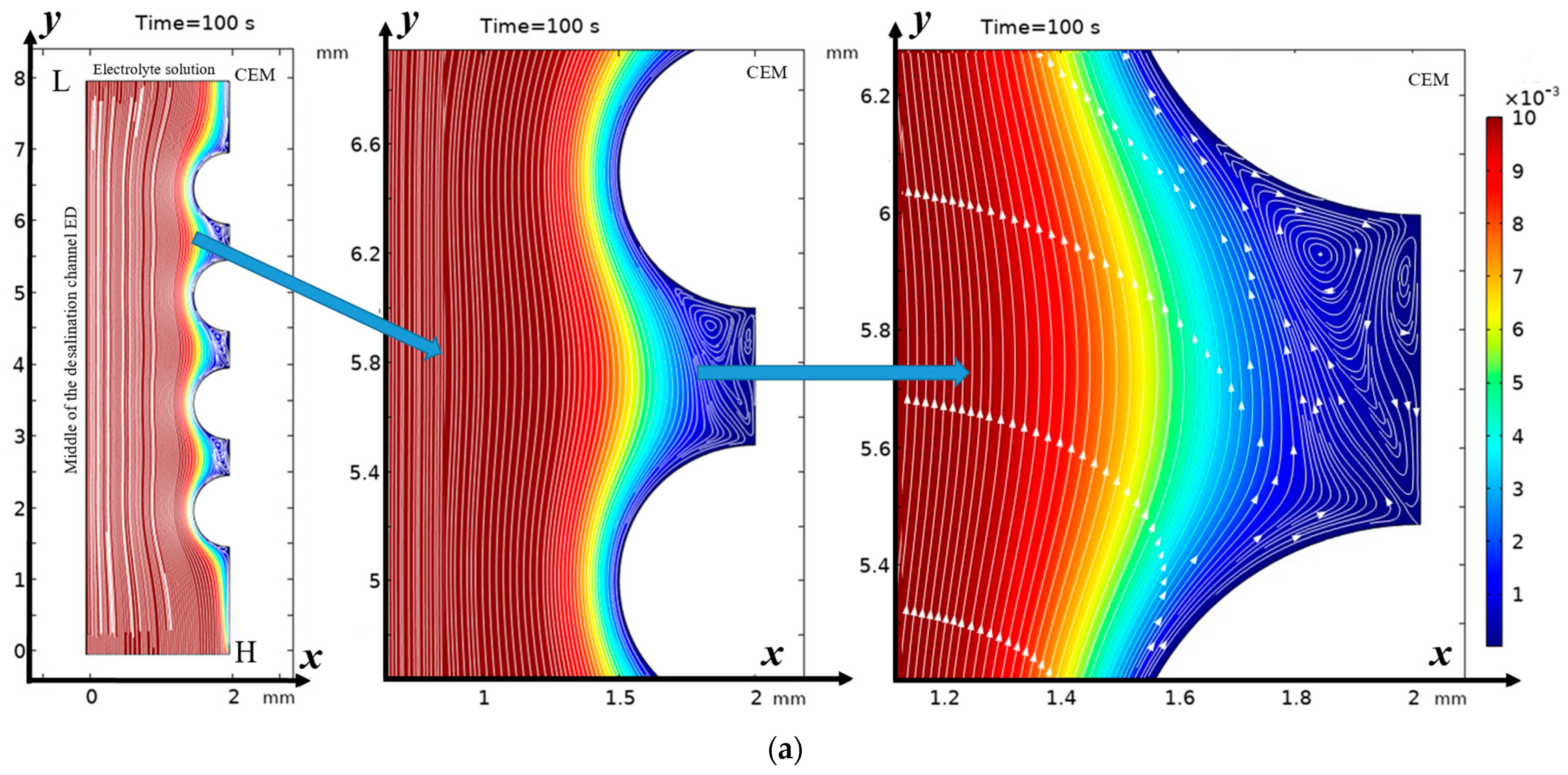
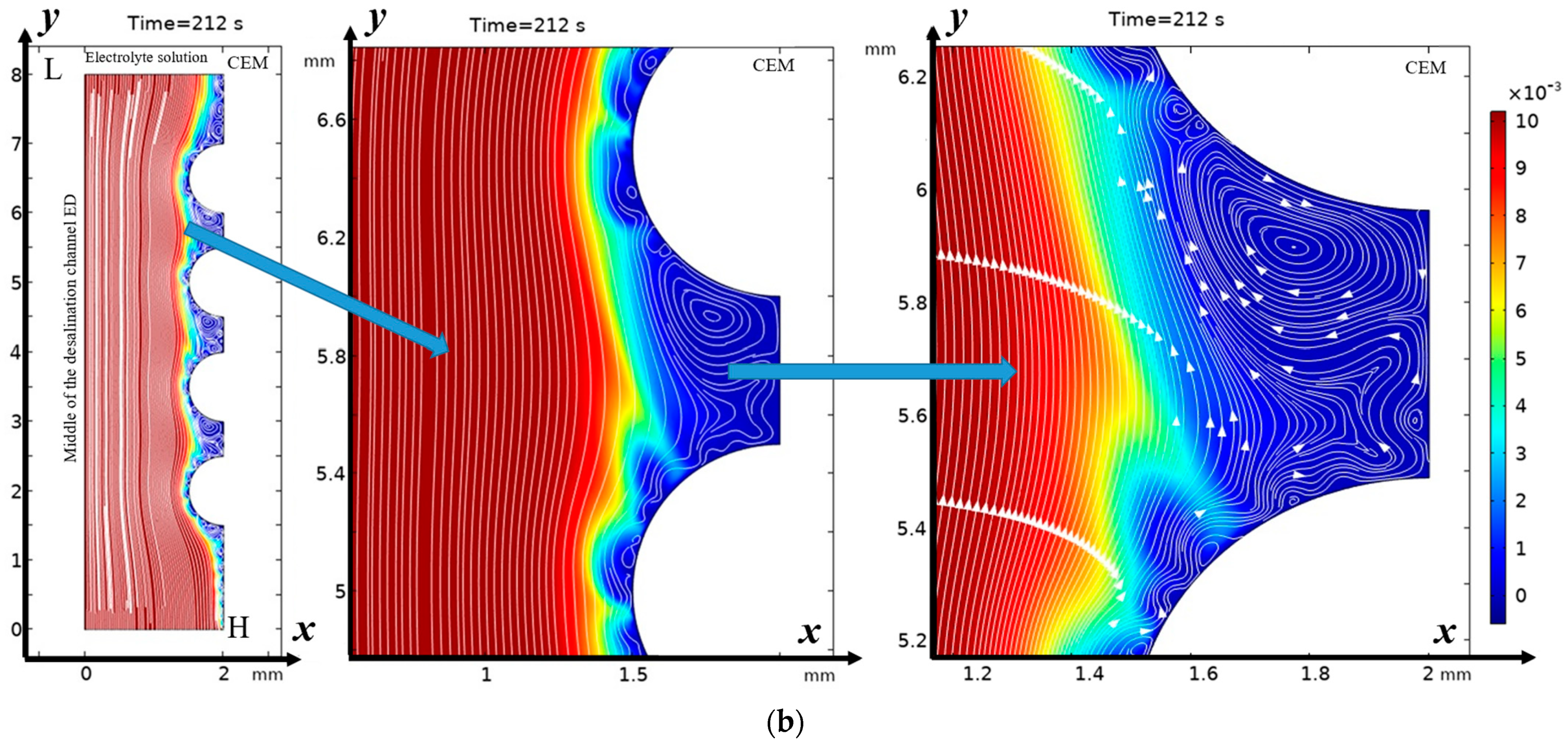
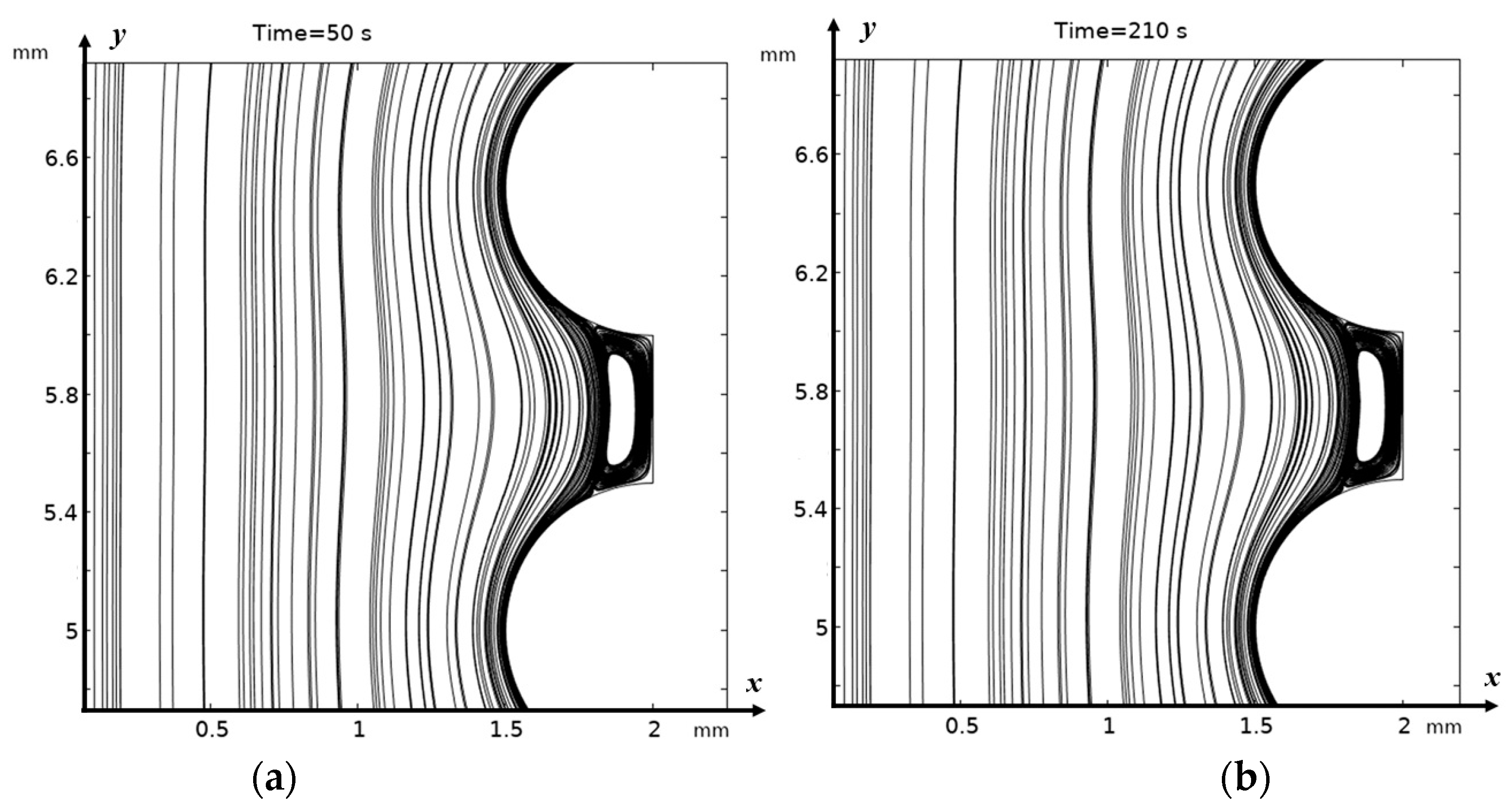
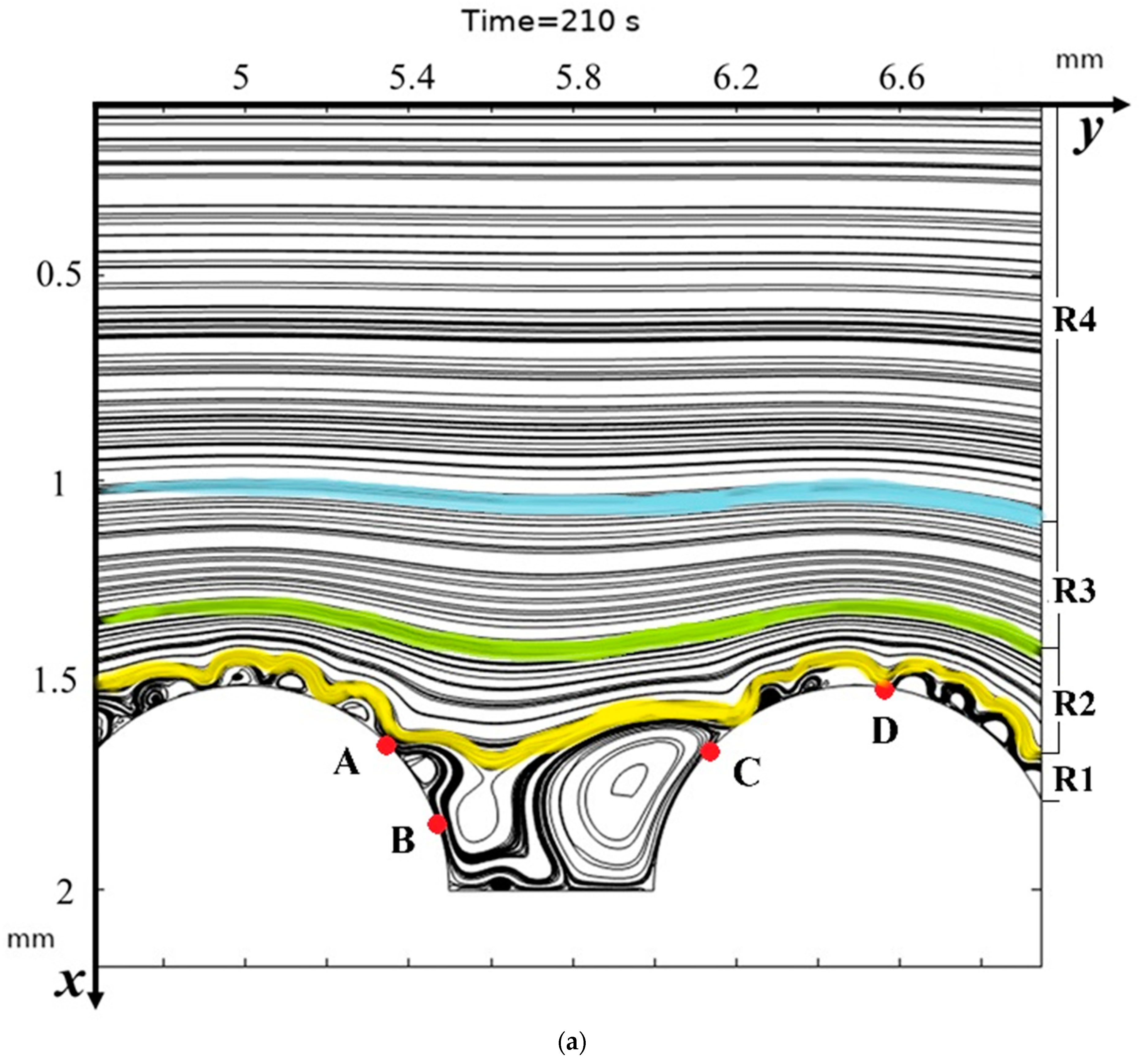
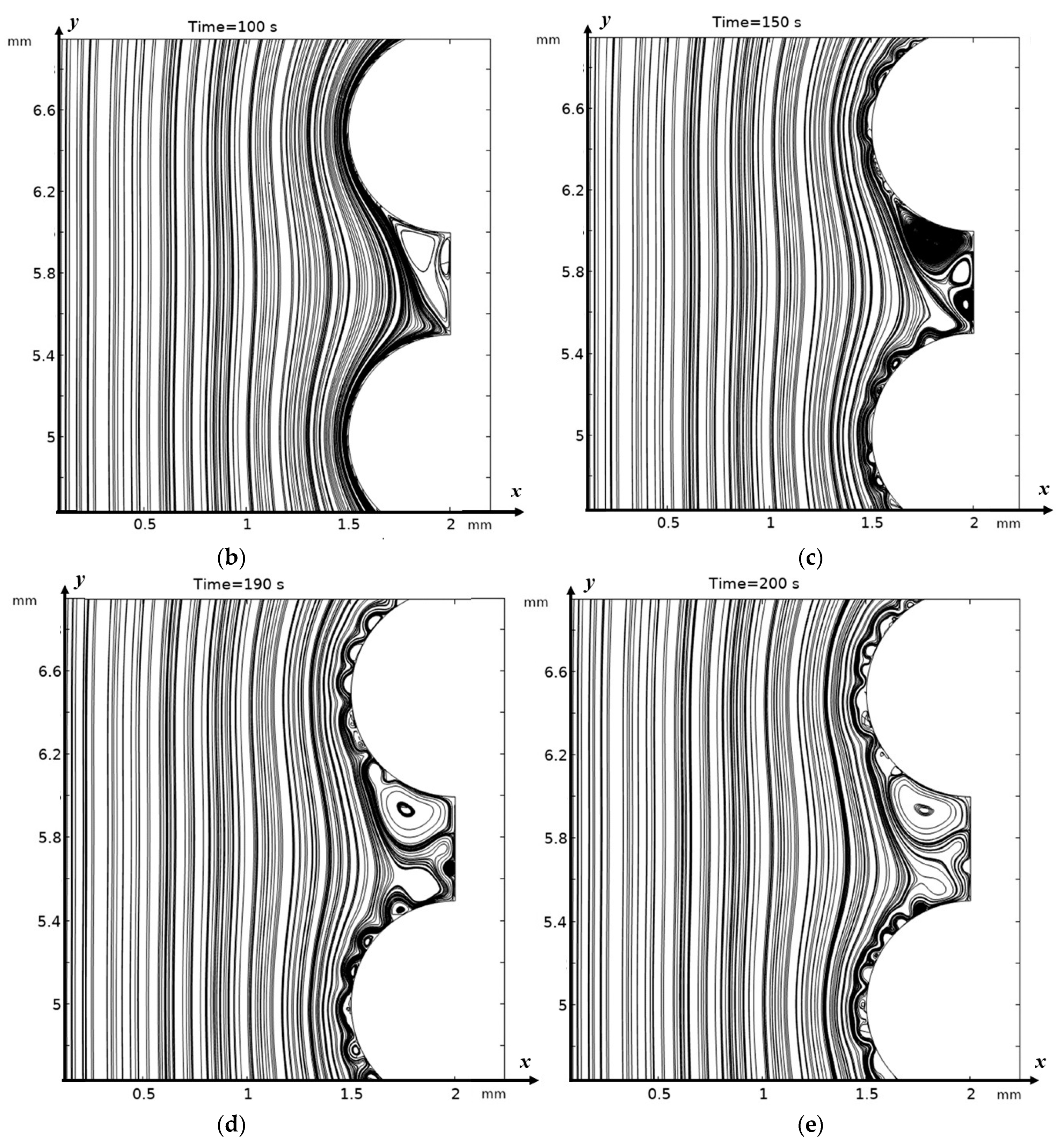
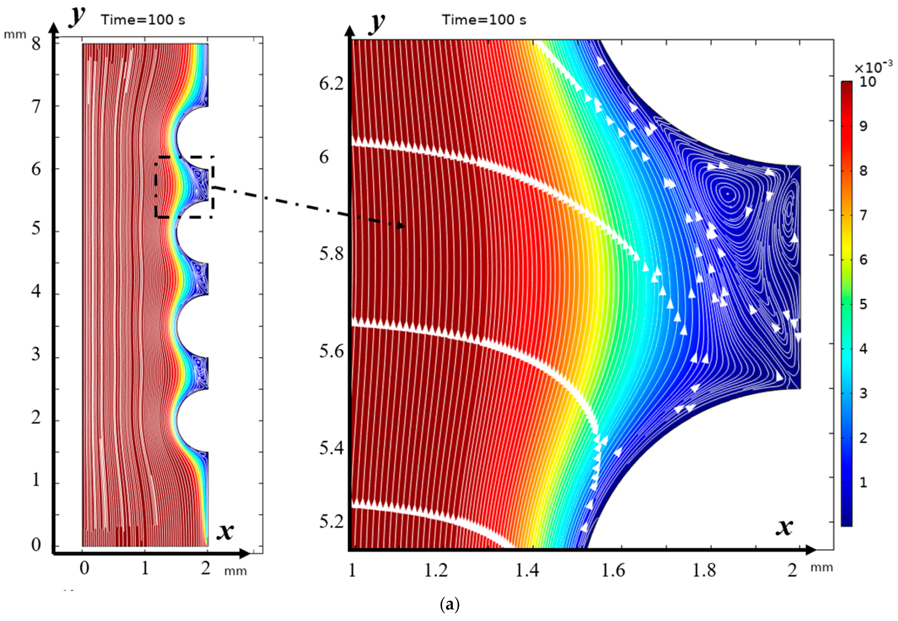
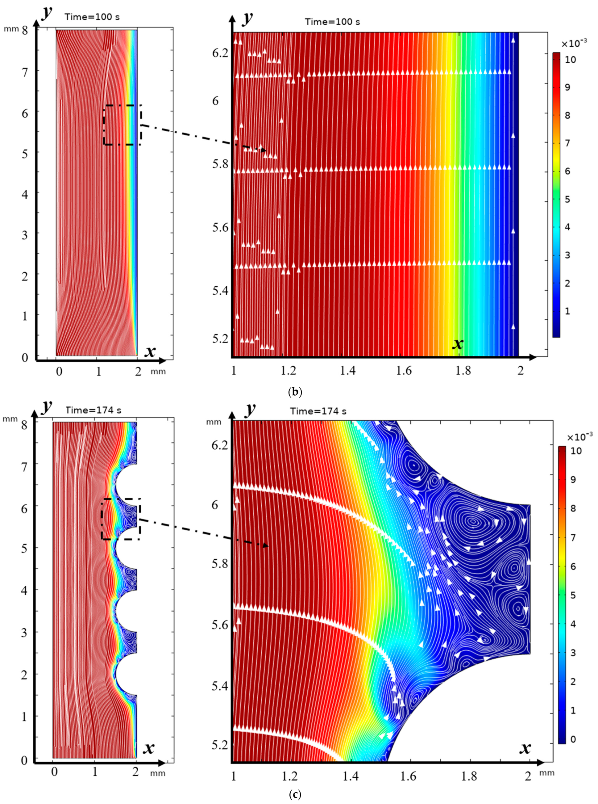
3.2. Structure of the Solution Flow

From Figure 2 it can be seen that “stagnant” zones are formed in the valleys between the hills, where the flow velocity is significantly lower, but the main change in the direction of the flow is towards the membrane, and the flow disturbance is noticeable almost to the core of the flow, but the zone of electroconvective vortices over most of the hill occupies a narrow strip. However, in the lower part of the hill and above the valley, the vortex zone significantly expands. Here, both electroconvective vortices and purely hydrodynamic vortices are formed.

In the absence of electroconvection, a steady state is reached in the valley fairly quickly, and a purely stagnant zone is formed (see Figure 3a,b). In the presence of electroconvection, electroconvective vortices penetrate the “stagnant” zone in the valley, carrying with them a more concentrated solution, which is desalinated in the valley, and flows out of it, carrying out the desalinated solution, i.e., this zone is no longer stagnant (Figure 4a). Electroconvective vortices and purely hydrodynamic vortices influence each other in a complex, nonlinear, and non-stationary manner; a change in the size and number of vortex structures, the formation of vortex clusters, and their bifurcation (Figure 4b–e) occur. Geometrical inhomogeneities (valleys) create zones where electroconvective vortices interact with hydrodynamic ones. This leads to enhanced mixing and accelerated removal of ions from the near-membrane region.

From Figure 4a, it is evident that the general structure of the flow, if moving across the channel, starting from the middle to the membrane, contains several regions: the flow core (in Figure 4a this region is designated as R4), where the flow is practically not disturbed and is a Poiseuille flow. Region R1, in which the streamlines are the envelopes of the vortex zone and are directly adjacent to the vortex zone. The region of curved flow—R2, which is enclosed between the envelopes and the flow core, is where the flow differs from the Poiseuille flow and where the solution streamlines are gradually deformed from the envelope streamlines to the Poiseuille streamlines—R3.

The structure of the flow directly above the hills and between the hills, i.e., below the region of the envelopes, has a different characteristic in three different regions (Figure 4a): in the upper slope of the hill to point A, in the lower slope of the hill to point B and in the valley itself between the hills (between points B and C). In the area between point A and after point C, there are no hydrodynamic vortices, and electroconvective vortices have the same structure as in the case of a membrane with a smooth surface (Figure 5). These areas are located in the upper part of the hill. In the lower part of the hill slope and the valley itself, the flow has a different character. In the lower part of the hill slope, two separation points are visible: the upper (point A) and the lower (point B), which is almost at the bottom. The left boundary of the lower part of the right slope of the hill is determined by the first separation point of the envelope of electroconvective vortices, and the right boundary is determined by the second separation point. The left boundary of the lower part of the left slope of the next hill is determined when the lower envelope approaches the hill surface at a distance approximately corresponding to the quasi-equilibrium SCR (point C). The right boundary is determined similarly to point D, where the upper envelope approaches the membrane. The flow above the valley itself, as noted above, is characterized by non-stationarity and instability, constant bifurcation of vortices due to the interaction of electroconvective and purely hydrodynamic vortices. Let us compare the distribution of concentrations (highlighted in color) and the solution streamlines for models with a structured surface (on the left in the figure) and without modification (on the right in the figure) at different moments in time (Figure 5).

It is evident from Figure 5a,b that from the very beginning, the region where concentrations change quite significantly is considerably wider at the surface of the modified membrane. This tendency is maintained further (Figure 5c,d). Moreover, the concentration of the solution drops considerably faster at the surface of the modified membrane (Figure 5). Thus, it is possible to conclude about the intensification of electroconvection and, accordingly, about the increase in the efficiency of desalination due to the modification of the membrane surface, including the increase in the conductive surface of the cation exchange membrane, which occurs during the modification of the membrane surface.

3.3. CVC and Its Description

In works [34,35,36], the authors derived and justified a special formula for calculating the theoretical current–voltage characteristic (CVC) of electromembrane systems (EMSs), based on the law of charge conservation in potentiodynamic mode. For a given one $t$, the potential drop is determined $\phi (t,H,y)=d_{\phi }\cdot t$ ($d_{\phi }$: speed of sweep of the potential drop). Solving the boundary value problem, we find the current density in the channel $\overrightarrow{I}(t,x,y)$. Then, to calculate the CVC, it is proposed to use the following formula:

$$i(t)={\displaystyle \frac{1}{HL}}{\displaystyle \underset{0}{\overset{H}{\int }}{\displaystyle \underset{0}{\overset{L}{\int }}{I}_x(t,s,y)dy}}ds+{\displaystyle \frac{1}{2HL}}{\displaystyle \underset{0}{\overset{L}{\int }}{\displaystyle \underset{0}{\overset{H}{\int }}(H-2x)div\overrightarrow{I}dxdy}}$$

(11)

We designate the following:

$$i_{av}(t)={\displaystyle \frac{1}{HL}}{\displaystyle \underset{0}{\overset{H}{\int }}{\displaystyle \underset{0}{\overset{L}{\int }}{I}_x(t,s,y)dy}}ds$$

(12)

$$i_d(t)={\displaystyle \frac{1}{2HL}}{\displaystyle \underset{0}{\overset{L}{\int }}{\displaystyle \underset{0}{\overset{H}{\int }}(H-2x)div\overrightarrow{I}dxdy}}.$$

(13)

Then, $i(t)=i_{av}(t)+i_d(t)$.

In [29,30,31], it is shown that the term $i_{av}(t)$ is the averaged conduction current carried by ions, and the second term $i_d(t)$ is the averaged displacement current.

Although the total current in the CVC calculation is not constant over time, its change can be made slow if the potential drop sweep rate is small. In this case $i_d(t)$, it is small, and when calculating the CVC, it is not necessary to take into account the bias current, and the CVC must be calculated using the formula $i_{av}(t)={\displaystyle \frac{1}{HL}}{\displaystyle \underset{0}{\overset{H}{\int }}{\displaystyle \underset{0}{\overset{L}{\int }}{I}_x(t,s,y)dy}}ds$.

In Figure 6, the abscissa shows the values of the potential drop, and the ordinate shows the current density value, dimensionless by the limiting diffusion current according to Leveck [34,35]: $i_{\lim }={\displaystyle \frac{FD{C}_0}{H\left(T_1-t_1\right)}}\left[1.47{\left({\displaystyle \frac{H^2{V}_0}{LD}}\right)}^{1/3}-0.2\right],T_1=1,t_1=0.5$.

As can be seen from Figure 6, the CVC in both cases has a classical form—a linear ohmic section, a “plateau”, and a secondary over-limiting rise associated with the onset and development of electroconvection. For models with a structured surface (blue color), the membrane is higher than the CVC of an unstructured (smooth) surface (red color), and, accordingly, the mass transport is higher.

A small convexity at the beginning of the “plateau” for the model with a structured surface is because it reacts more sensitively to changes in the potential sweep rate, i.e., it is more sensitive to non-stationarity effects.

3.4. Verification of Results

To verify the results, a comparison was made with the experiment described in [18]. In this work, images of its section in the swollen state were taken, which were used to model the cation-exchange membrane. Images of electroconvective vortices arising in a depleted solution near the membranes at a current of i = 2.4 mA and t = 22 ± 1 s show that the average size of the vortex structures of the unprofiled membrane is approximately 200 μm, while for the profiled membrane it is approximately one and a half times larger, i.e., about 300 μm. This is in good qualitative and quantitative agreement with the numerical results.

• Electroconvective vortex sizes: Average diameter and spatial distribution. Vortex sizes: Numerical result: 280 ± 30 μm. Experiment: 300 ± 40 μm. Discrepancy: 6.7%, which is within the measurement error.
• Steady-state mode establishment time: From the start of voltage application to current stabilization. Time to establish the mode: Numerical: 120 s. Experimental: 130 ± 10 s.
• Concentration profile at the membrane: Concentration gradient at a distance of 0–200 μm from the surface. Concentration profile: Coefficient of determination: R² = 0.92.

4. Conclusions

The 2D mathematical model of the transport process in half of the desalination channel with the geometric modification of the surface by the cation-exchange membrane is constructed based on the boundary value problem for the coupled system of Nernst–Planck–Poisson and Navier–Stokes equations. A numerical modeling of the effect of geometric modification of the surfaces of ion-exchange membranes on the transport of salt ions was carried out, and the main patterns of salt ion transport were established, taking into account diffusion, electromigration, forced convection, and electroconvection. Using the current–voltage characteristics, it was shown that the geometric modification of the surface of ion-exchange membranes enhances the transport of salt ions.

The geometric modification of the ion-exchange membrane surface (semicircular protrusions 200 μm high) increases the active zone area by 35%, which leads to the formation of stable electroconvective vortices. This reduces concentration polarization by 40% and increases the ion transport rate by 1.5 times compared to smooth membranes.

The interaction of electroconvective and hydrodynamic vortices in the valleys between inhomogeneities destroys stagnant zones, reducing the desalination time by 28% (from 280 to 200 s for 90% purification).

Structured membranes demonstrate a steeper rise in secondary current in the region of superlimit modes, which allows for a reduction in the operating voltage by 15% while maintaining productivity.

Recommendations for membrane design include the use of semicircular protrusions with a pitch of 500 μm and a height of 200 μm, which overall ensures a balance between efficiency and hydrodynamic resistance.

Promising research areas include the following:

-

Study of the influence of three-dimensional structures (pyramids and spirals) on turbulence and mass transfer.

-

Analysis of the interaction of vortices in adjacent channels.

-

Development of machine learning algorithms (e.g., genetic algorithms) to find the optimal geometry taking into account conflicting requirements, such as the minimization of resistance, maximization of area, and resistance to contamination.

-

Accounting for the dissociation/recombination of water molecules.

5. Definitions of Key Terms

1.

Electromembrane Systems (EMSs)

These are systems that use ion-exchange membranes and an electric field to separate ions in solutions. They are used in water desalination, wastewater treatment, and electrochemical processes [1,7].

2.

Electroconvection

This refers to the movement of an electrolyte caused by the action of an external electric field on the spatial charge in the double electric layer (DEL) at the membrane surface. It is divided into two types:

-

Electroconvection of the first kind: fluid movement caused by the equilibrium DEL.

-

Electroconvection of the second kind: movement caused by the expansion of the DEL under strong membrane polarization [9,10].

3.

Geometric modification of membranes

This refers to changing the surface of ion exchange membranes (e.g., creating protrusions, valleys, or fractal structures) to control mass transfer. Examples include semicircular protrusions and diamond-shaped nodes [17,25,31].

4.

Potentiodynamic mode

This refers to the EMS operating mode in which the potential difference across the membrane changes at a constant rate (e.g., 0.005 V/s). It is used to analyze current–voltage characteristics [7,34].

5.

Concentration polarization

This refers to changing the concentration of ions at the membrane surface due to the difference in their transport rates in the solution and the membrane. It leads to a decrease in the efficiency of EMSs.

6.

Ion exchange membrane (CEM/AEM)

-

Cation exchange membrane (CEM): a membrane that selectively passes cations due to fixed negative charges.

-

Anion exchange membrane (AEM): a membrane that selectively transmits anions due to fixed positive charges [27,30].

7.

Spatial electrical force

This refers to the force acting on the volume charge in a solution. It is modeled as the term $f=\rho E$ in the Navier–Stokes equation, where $\rho$ is the charge density, and $E$ is the electric field strength [7,11].

8.

Peclet number (Pe)

This is a dimensionless parameter that characterizes the ratio of convective and diffusive transport, $Pe=V_{0}H/D$, where $V_0$ is the flow velocity, $H$ is the characteristic size, and $D$ is the diffusion coefficient [8].

9.

Reynolds number (Re)

This dimensionless parameter reflects the relationship between inertial and viscous forces and determines the flow regime of a liquid, $Re=V_{0}H/\nu$, where $\nu$ is the kinematic viscosity. At $Re<2000$, the flow is laminar [8].

10.

Current–voltage characteristic (CVC)

This refers to current density as a function of the applied potential jump and includes three sections: ohmic, plateau (diffusion limitation), and superlimit growth (the activation of electroconvection) [34,35,36].

References

1. Menachem, E.; William, P. The Future of Seawater Desalination: Energy, Technology, and the Environment. Science 2011, 333, 712–717. [Google Scholar] [CrossRef]
2. Sun, Y.; Tan, X.; Xiang, B.; Gong, J.; Li, J. Solar-driven interfacial evaporation for sustainable desalination: Evaluation of current salt-resistant strategies. Chem. Eng. J. 2023, 474, 145945. [Google Scholar] [CrossRef]
3. Wang, J.; Huo, E. Opportunities and Challenges of Seawater Desalination Technology. Front. Energy Res. 2022, 10, 960537. [Google Scholar] [CrossRef]
4. Jay, W.; Menachem, E. Materials for Next-Generation Desalination and Water Purification Membranes. Nat. Rev. Mater. 2016, 1, 16018. [Google Scholar] [CrossRef]
5. Deng, D.; Dydek, E.; Han, J.; Schlumpberger, S.; Mani, A.; Zaltzman, B.; Bazant, M.Z. Overlimiting Current and Shock Electrodialysis in Porous Media. Langmuir ACS J. Surf. Colloids 2013, 29, 16167–16177. [Google Scholar] [CrossRef]
6. Mani, A.; Wang, K.M. Electroconvection Near Electrochemical Interfaces: Experiments, Modeling, and Computation. Annu. Rev. Fluid Mech. 2020, 52, 509–529. [Google Scholar] [CrossRef]
7. Utenov, M.K.; Uzdenova, A.M.; Kovalenko, A.; Nikonenko, V.V.; Pismenskaya, N.D.; Vasil, V.I.; Sistat, P.; Pourcelly, G. Basic mathematical model of overlimiting transport enhanced by electroconvection in flow-through electrodialysis membrane cells. J. Memb. Sci. 2013, 447, 190–202. [Google Scholar] [CrossRef]
8. Probstein, R.F. Physicochemical Hydrodynamics: An Introduction; John Wiley and Sons Inc.: New York, NY, USA, 1994; 416p. [Google Scholar]
9. Dukhin, S.S. Electrokinetic phenomena of the second kind and their applications. Adv. Colloid Interface Sci. 1991, 35, 173–196. [Google Scholar] [CrossRef]
10. Rubinstein, I.; Shtilman, L. Voltage against current curves of cation exchange membranes. J. Chem. Soc. Faraday Trans. 1979, 75, 231. [Google Scholar] [CrossRef]
11. Urtenov, M.A.; Kirillova, E.V.; Seidova, N.M.; Nikonenko, V.V. Decoupling of the Nernst-Planck and Poisson equations. Application to a membrane system at overlimiting currents. J Phys Chem B. 2007, 111, 14208–14222. [Google Scholar] [CrossRef]
12. Abu-Rjal, R.; Leibowitz, N.; Park, S.; Zaltzman, B.; Rubinstein, I.; Yossifon, G. Signature of electroconvective instability in transient galvanostatic and potentiostatic modes in a microchannel-nanoslot device. Phys. Rev. Fluids 2019, 4, 084203. [Google Scholar] [CrossRef]
13. Li, G.; Townsend, A.; Archer, L.A.; Koch, D.L. Electroconvection near an ion-selective surface with Butler–Volmer kinetics. J. Fluid Mech. 2022, 930, A26. [Google Scholar] [CrossRef]
14. Kim, J.; Davidson, S.M.; Mani, A. Characterization of chaotic electroconvection near flat inert electrodes under oscillatory voltages. Micromachines 2019, 10, 161. [Google Scholar] [CrossRef] [PubMed]
15. Demekhin, E.A.; Ganchenko, G.S.; Kalaydin, E.N. Transition to electrokinetic instability near imperfect charge-selective membranes. Phys. Fluids 2018, 30, 082006. [Google Scholar] [CrossRef]
16. Choi, J.; Cho, M.; Shin, J.; Kwak, R.; Kim, B. Electroconvective instability at the surface of one-dimensionally patterned ion exchange membranes. J. Membr. Sci. 2024, 691, 122256. [Google Scholar] [CrossRef]
17. Stockmeier, F.; Stüwe, L.; Kneppeck, C.; Musholt, S.; Albert, K.; Linkhorst, J.; Wessling, M. On the interaction of electroconvection at a membrane interface with the bulk flow in a spacer-filled feed channel. J. Membr. Sci. 2023, 678, 121589. [Google Scholar] [CrossRef]
18. Bräsel, B.; Yoo, S.-W.; Huber, S.; Wessling, M.; Linkhorst, J. Evolution of particle deposits at communicating membrane pores during crossflow filtration. J. Membr. Sci. 2023, 686, 121977. [Google Scholar] [CrossRef]
19. Seo, M.; Kim, W.; Lee, H.; Kim, S.J. Non-negligible effects of reinforcing structures inside ion exchange membrane on stabilization of electroconvective vortices. Desalination 2022, 538, 115902. [Google Scholar] [CrossRef]
20. Ugrozov, V.V.; Filippov, A.N. Resistance of an Ion-Exchange Membrane with a Surface-Modified Charged Layer. Colloid J. 2022, 84, 761–768. [Google Scholar] [CrossRef]
21. Filippov, A.N.; Akberova, E.M.; Vasil’eva, V.I. Study of the Thermochemical Effect on the Transport and Structural Characteristics of Heterogeneous Ion-Exchange Membranes by Combining the Cell Model and the Fine-Porous Membrane Model. Polymers 2023, 15, 3390. [Google Scholar] [CrossRef]
22. Rubinstein, I.; Zaltzman, B. How the fine structure of the electric double layer and the flow affect morphological instability in electrodeposition. Phys. Rev. Fluids 2023, 8, 093701. [Google Scholar] [CrossRef]
23. Pismenskaya, N.; Gorobchenko, A.; Solonchenko, K.; Nikonenko, V. Effect of current density on anion-exchange membrane scaling during electrodialysis of phosphate-containing solution: Experimental study and predictive simulation. Desalination 2025, 600, 118487. [Google Scholar] [CrossRef]
24. Hopsort, G.; Cacciuttolo, Q.; Pasquier, D. Electrodialysis as a key operating unit in chemical processes: From lab to pilot scale of latest breakthroughs. Chem. Eng. J. 2024, 494, 153111. [Google Scholar] [CrossRef]
25. Zabolotskii, V.I.; Loza, S.A.; Sharafan, M.V. Physicochemical properties of profiled heterogeneous ion-exchange membranes. Elektrokhimiya 2005, 41, 1185–1192. [Google Scholar] [CrossRef]
26. Gnusin, N.P.; Pevnitskaya, M.V.; Varentsov, V.K.; Grebenyuk, V.D. USSR Inventor’s Certificate. Byull. Izobret. 1971, 35, 216622. [Google Scholar]
27. Larchet, C.; Zabolotsky, V.I.; Pismenskaya, N.; Nikonenko, V.V.; Tskhay, A.; Tastanov, K.; Pourcelly, G. Comparison of different ED stack conceptions when applied for drinking water production from brackish waters. Desalination 2008, 222, 489–496. [Google Scholar] [CrossRef]
28. Vasil’eva, V.; Goleva, E.; Pismenskaya, N.; Kozmai, A.; Nikonenko, V. Effect of surface profiling of a cation-exchange membrane on the phenylalanine and NaCl separation performances in diffusion dialysis. Sep. Purif. Technol. 2019, 210, 48–59. [Google Scholar] [CrossRef]
29. Loza, S.; Loza, N.; Kutenko, N.; Smyshlyaev, N. Profiled Ion-Exchange Membranes for Reverse and Conventional Electrodialysis. Membranes 2022, 12, 985. [Google Scholar] [CrossRef]
30. Melnikov, S.; Loza, S.; Sharafan, M.; Zabolotskiy, V. Electrodialysis treatment of secondary steam condensate obtained during production of ammonium nitrate. Technical and economic analysis. Sep. Purif. Technol. 2016, 157, 179–191. [Google Scholar] [CrossRef]
31. Liu, J.; Geise, G.M.; Luo, X.; Hou, H.; Zhang, F.; Feng, Y.; Hickner, M.A.; Logan, B.E. Patterned ion exchange membranes for improved power production in microbial reverse-electrodialysis cells. J. Power Sources 2014, 271, 437–443. [Google Scholar] [CrossRef]
32. Stockmeier, F.; Felder, D.; Eser, S.; Habermann, M.; Peric, P.; Musholt, S.; Albert, K.; Linkhorst, J.; Wessling, M. Localized Electroconvection at Ion-Exchange Membranes with Heterogeneous Surface Charge. Res. Sq. 2021. [Google Scholar] [CrossRef]
33. Xu, Y.; Chuah, C.Y.; Yang, Z.; Yuan, S. 3D Printed Functional Membranes for Water Purification; The Royal Society of Chemistry: London, UK, 2021; Chapter 11. [Google Scholar] [CrossRef]
34. Kovalenko, A.; Urtenov, M. Analysis of the theoretical CVC of electromembrane systems. E3S Web Conf. 2020, 224, 02010. [Google Scholar] [CrossRef]
35. Urtenov, M.K.; Kovalenko, A.V.; Sukhinov, A.I.; Chubyr, N.O.; Gudza, V.A. Model and numerical experiment for calculating the theoretical current-voltage characteristic in electro-membrane systems. IOP Conf. Ser. Mater. Sci. Eng. 2019, 680, 012030. [Google Scholar] [CrossRef]
36. Kirillova, E.; Kovalenko, A.; Urtenov, M. Study of the Current–Voltage Characteristics of Membrane Systems Using Neural Networks. AppliedMath 2025, 5, 10. [Google Scholar] [CrossRef]
Figure 1. Scheme of half of desalination channel with geometrically modified surface of cation exchange membrane (a)—The considered area is half of the flow channel of desalination of ED with cation exchange membrane (CEM), where x is the coordinate normal to the membrane surface, changing from 0 (center of the channel) to H (boundary with CEM); y is the coordinate tangent to the membrane surface, changing from 0 (entrance to the channel) to L (exit) from the channel. Half of the channel is highlighted in gray, the membrane is on the right, solution is fed into the channel from below. Alternating convex geometric inhomogeneities in the form of semicircles are highlighted on the CEM surface. (b)—Half of the channel, as in the first, with the same volumetric flow rate and concentration, but without structural inhomogeneity of the membrane surface. On the structured membrane surface, the no-slip condition is specified, and on the smooth surface (Figure 1b), the velocity symmetry along the X axis is specified.
Mathematics 13 01523 g001
Figure 2. Solution streamlines and cation concentration distribution (highlighted in color; scale on the right) at (a) 100 s (0.5 V) and (b) 212 s (1.06 V): on the left—general view, in the center—first magnification of a fragment (two hills and a valley between them), and on the right—second magnification—streamlines and concentration distribution over the valley. Vortex zones are located in areas of low concentration (blue color). The arrows indicate the direction of rotation of the vortices. The figure shows areas with swirling flows, where the arrows indicate the movement of the fluid clockwise or counterclockwise.
Mathematics 13 01523 g002aMathematics 13 01523 g002b
Figure 3. Solution streamlines at (a) 50 s (0.25 V); (b) 210 s for the absence of external electrical force, i.e., for purely hydrodynamic flow.
Mathematics 13 01523 g003
Figure 4. Solution streamlines at different times: (a)—flow structures at 210 s (1.05 V); change in flow structure over time (b)—100 s, (c)—150 s, (d)—190 s, and (e)—200 s.
Mathematics 13 01523 g004aMathematics 13 01523 g004b
Figure 5. Distribution of concentrations (highlighted in color) and solution streamlines for models with a structured surface (a,c) and an unstructured smooth surface (b,d) at different times of (a,b) 100 s (0.5 V), and (b,d) 174 s (0.87 V). Vortex zones are located in areas of low concentration (blue color). The arrows indicate the direction of rotation of the vortices. The figure shows areas with swirling flows, where the arrows indicate the movement of the fluid clockwise or counterclockwise.
Mathematics 13 01523 g005aMathematics 13 01523 g005bMathematics 13 01523 g005c
Figure 6. CVC for models with a structured surface (blue) and an unstructured (smooth) surface (orange).
Mathematics 13 01523 g006
Disclaimer/Publisher’s Note: The statements, opinions and data contained in all publications are solely those of the individual author(s) and contributor(s) and not of MDPI and/or the editor(s). MDPI and/or the editor(s) disclaim responsibility for any injury to people or property resulting from any ideas, methods, instructions or products referred to in the content.