
Tensor-Based Uncoupled and Incomplete Multi-View Clustering

Abstract
1. Introduction
- Unlike existing IMVC models, we integrate missing view recovery with the coupling of cross-view self-representation matrices. This approach not only uncovers the latent information of missing samples but also reduces the interference caused by uncoupled data.
- An algorithm based on the alternating direction method of multipliers (ADMM) [18] is designed to solve the proposed TUIMC. Extensive experiments are conducted on various datasets, showcasing the efficiency of the proposed model.
2. Problem Background and Preparations
2.1. Notation and Descriptions
2.2. Definitions
2.3. Related Works
2.3.1. Self-Representation Learning
2.3.2. Missing Sample Recovery
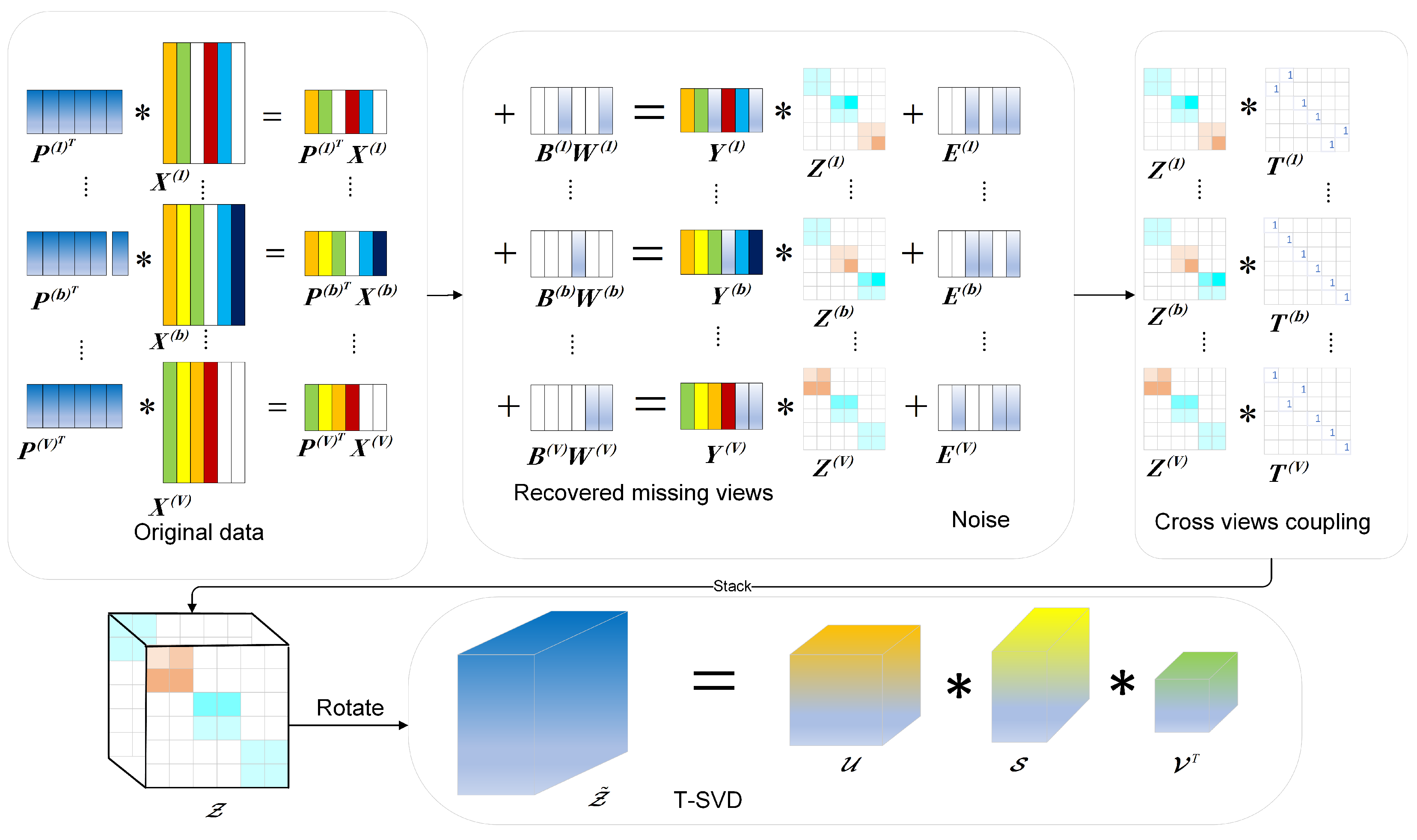
3. Methodology
3.1. Primary Motivations
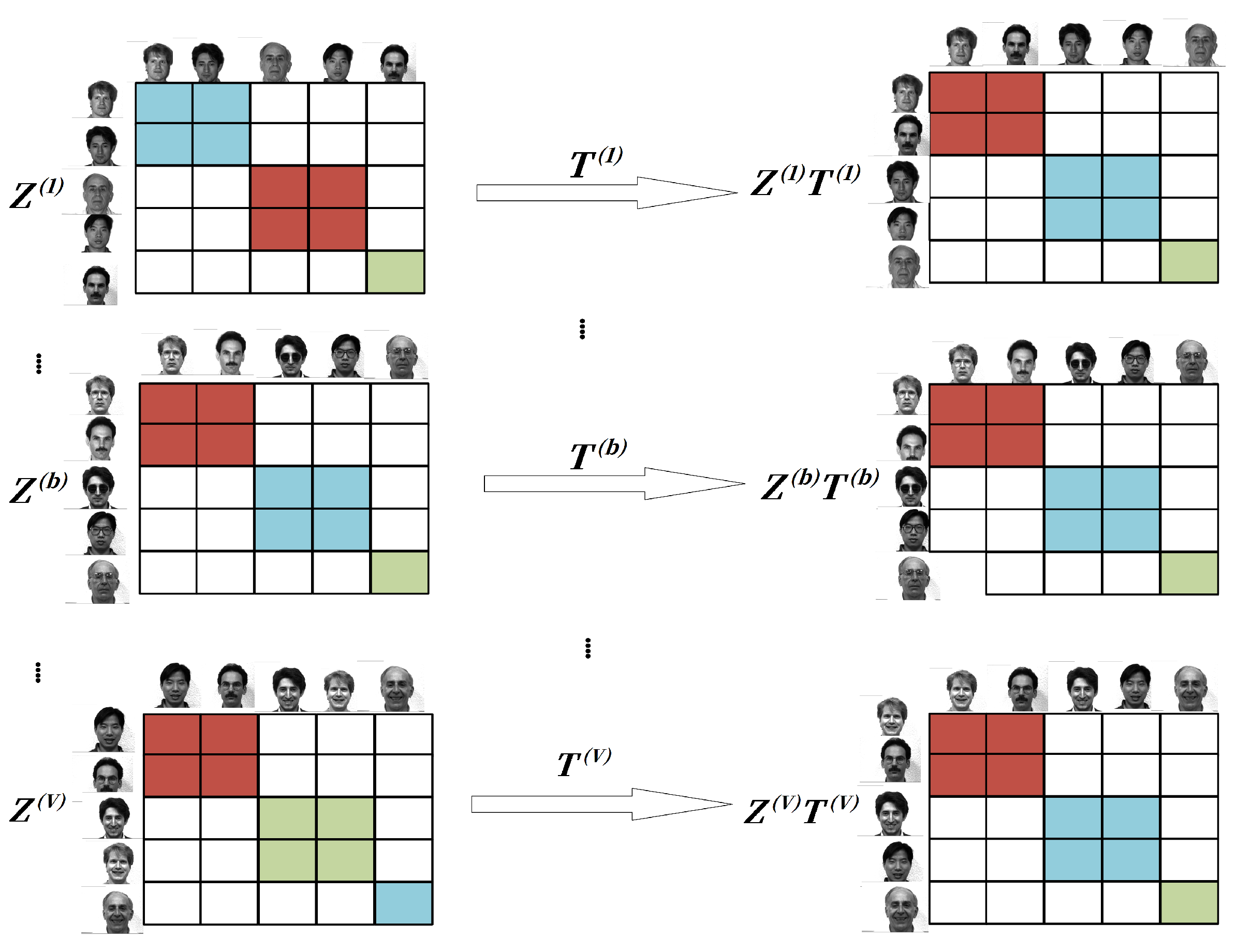
3.1.1. Cross-View Coupling
3.1.2. Joint Low-Dimensional Subspace Learning and Sample Recovery
3.2. The Proposed Model
3.3. Optimization
| Algorithm 1 TUIMC for multi-view clustering. |
| Input: Incomplete multi-view data: , the index matrices , , , dimensionality reduction k, and the index b of the template view.
Initialize: , , , , , , , , . while not convergence do 1. Update by Equation (23); 2. Update by Equation (25); 3. Update by Equation (9); 4. Update by Equation (12); 5. Update by Equation (15); 6. Update by Equation (20); 7. Update by Equation (33); 8. Update by Equation (34); 9. Update by Equation (29); 10. Update = ; 11. Update by Equation (31); 12. Update by Equation (35); 13. Update parameter by Equation (36); 14. Check the convergence condition (37); 15. until Convergence 16. Obtain the clustering results using the spectral clustering method on the affinity matrix . end |
3.4. Complexity Analysis
4. Experimental Results and Analysis
4.1. Multi-View Datasets
4.2. Incomplete Data Construction
4.3. Comparative Models
4.4. Evaluation Metrics
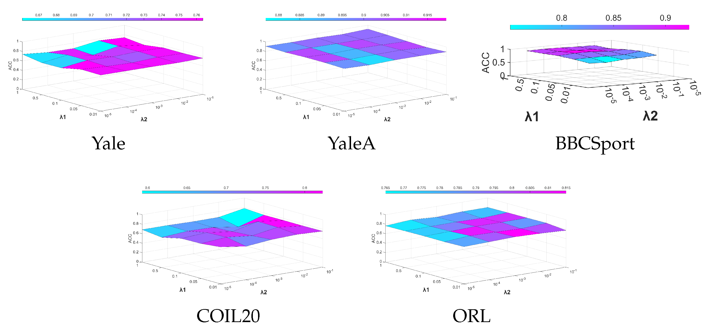
4.5. Parameter Settings
4.6. Experimental Results
- The experiments are tested on five real-world datasets, and the results suggest that the model outperforms nine existing multi-view clustering methods in most cases, including two for coupled data and seven for uncoupled data. Specifically, in terms of ACC, NMI, purity, Fscore, and precision, TUIMC performed well.
- Comparison with graph-based methods: The proposed method achieves outstanding clustering results in five evaluation metrics on the five datasets. Essentially, all the metrics are higher than those of the comparison methods. For example, on the Yale dataset with a missing rate of , the ACC, NMI, and purity of the proposed method are , , and higher than those of HCLS-CGL, respectively. Comparison with anchor-based methods: On the five datasets, all metrics are higher than those of SIMVC. For example, on the ORL dataset with a missing rate of , the ACC, NMI, and purity of the proposed model are, respectively, , , and higher than those of SIMVC. Comparison with subspace-based methods: On the five datasets, all the metrics are higher than those of IMSR. This demonstrates that the proposed method exhibits superior performance compared to alignment-oriented approaches.
- Comparison with uncoupled methods: On the COIL20 dataset with a missing rate of , the ACC, NMI, and purity are, respectively, , , and higher than those of T-UMC. For MVC-UM, all the metrics for TUIMC are higher than MVC-UM’s corresponding metrics. This indicates that the proposed method still maintains superiority compared to the uncoupled methods, likely due to the fact that these uncoupled methods do not specifically address the challenges of incomplete data.
4.7. Analysis of Running Time
4.8. Parameter Sensitivity
4.9. Ablation Study
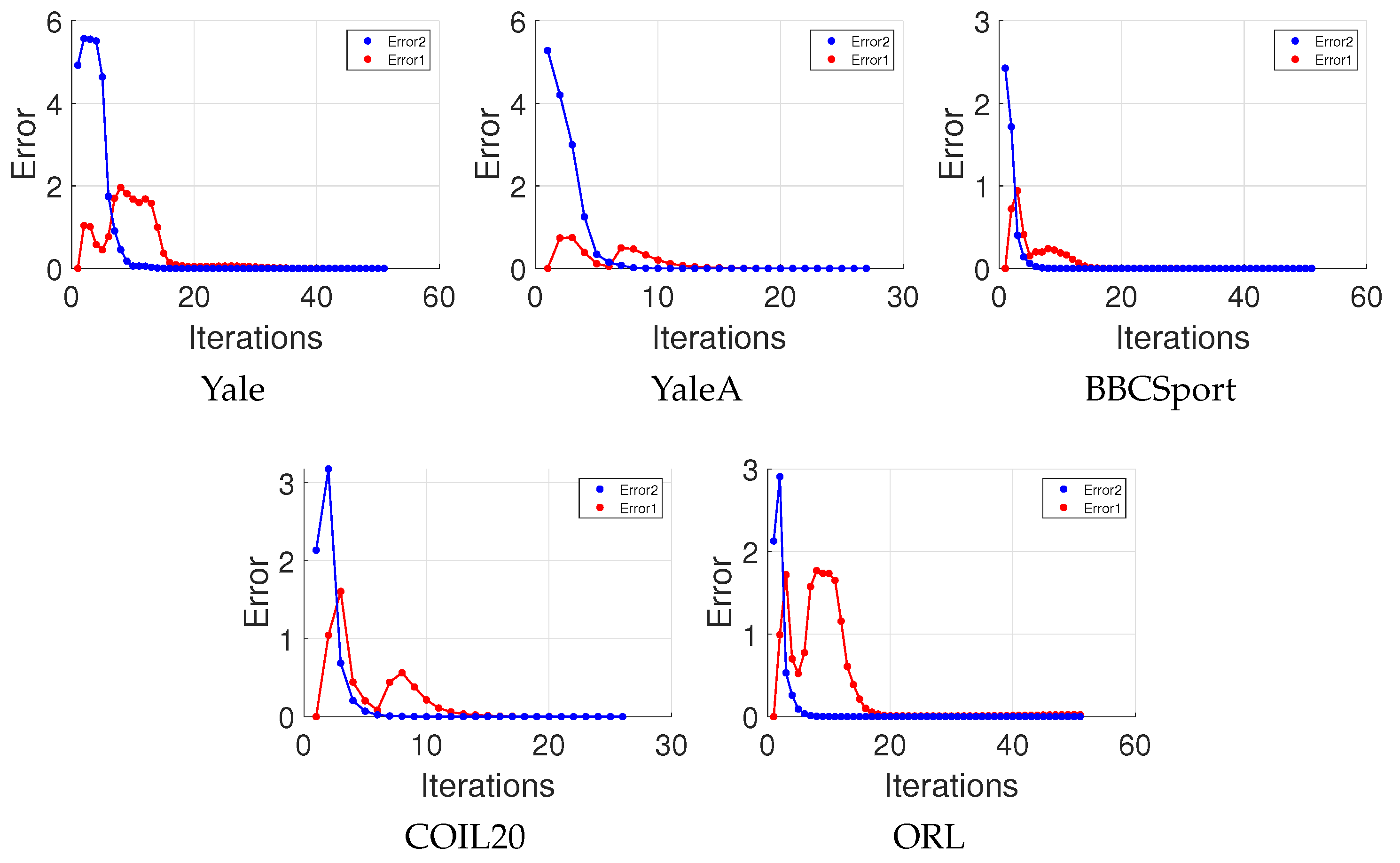
4.10. Convergence Study
5. Conclusions
Author Contributions
Funding
Data Availability Statement
Conflicts of Interest
References
- Ren, Y.; Chen, X.; Xu, J.; Pu, J.; Huang, Y.; Pu, X.; Zhu, C.; Zhu, X.; Hao, Z.; He, L. A novel federated multi-view clustering method for unaligned and incomplete data fusion. Inf. Fusion 2024, 108, 102357. [Google Scholar] [CrossRef]
- Guo, W.; Che, H.; Leung, M.F. Tensor-Based Adaptive Consensus Graph Learning for Multi-View Clustering. IEEE Trans. Consum. Electron. 2024, 70, 4767–4784. [Google Scholar] [CrossRef]
- Guo, W.; Che, H.; Leung, M.F.; Jin, L.; Wen, S. Robust Mixed-order Graph Learning for incomplete multi-view clustering. Inf. Fusion 2025, 115, 102776. [Google Scholar] [CrossRef]
- Guo, W.; Che, H.; Leung, M.F. High-order consensus graph learning for incomplete multi-view clustering. Appl. Intell. 2025, 55, 521. [Google Scholar] [CrossRef]
- Han, Q.; Hu, L.; Gao, W. Feature relevance and redundancy coefficients for multi-view multi-label feature selection. Inf. Sci. 2024, 652, 119747. [Google Scholar] [CrossRef]
- Hu, X.; Li, Z.; Wu, Y.; Liu, J.; Luo, X.; Ren, J. Neighbouring-slice Guided Multi-View Framework for brain image segmentation. Neurocomputing 2024, 575, 127315. [Google Scholar] [CrossRef]
- Wan, X.; Liu, J.; Gan, X.; Liu, X.; Wang, S.; Wen, Y.; Wan, T.; Zhu, E. One-step multi-view clustering with diverse representation. IEEE Trans. Neural Netw. Learn. Syst. 2024, 36, 5774–5789. [Google Scholar] [CrossRef]
- Che, H.; Pan, B.; Leung, M.F.; Cao, Y.; Yan, Z. Tensor factorization with sparse and graph regularization for fake news detection on social networks. IEEE Trans. Comput. Soc. Syst. 2023, 11, 4888–4898. [Google Scholar] [CrossRef]
- Pan, B.; Li, C.; Che, H.; Leung, M.F.; Yu, K. Low-rank tensor regularized graph fuzzy learning for multi-view data processing. IEEE Trans. Consum. Electron. 2023, 70, 2925–2938. [Google Scholar] [CrossRef]
- Kilmer, M.E.; Braman, K.; Hao, N.; Hoover, R.C. Third-order tensors as operators on matrices: A theoretical and computational framework with applications in imaging. SIAM J. Matrix Anal. Appl. 2013, 34, 148–172. [Google Scholar] [CrossRef]
- Yang, M.S.; Sinaga, K.P. Federated Multi-View K-Means Clustering. IEEE Trans. Pattern Anal. Mach. Intell. 2024, 47, 2446–2459. [Google Scholar] [CrossRef] [PubMed]
- Pu, X.; Che, H.; Pan, B.; Leung, M.F.; Wen, S. Robust weighted low-rank tensor approximation for multiview clustering with mixed noise. IEEE Trans. Comput. Soc. Syst. 2023, 11, 3268–3285. [Google Scholar] [CrossRef]
- Shen, Q.; Zhang, X.; Wang, S.; Li, Y.; Liang, Y.; Chen, Y. Dual Completion Learning for Incomplete Multi-View Clustering. IEEE Trans. Emerg. Top. Comput. Intell. 2024, 9, 455–467. [Google Scholar] [CrossRef]
- Hu, M.; Chen, S. Doubly aligned incomplete multi-view clustering. In Proceedings of the 27th International Joint Conference on Artificial Intelligence, Stockholm, Sweden, 13–19 July 2018; pp. 2262–2268. [Google Scholar]
- Yu, H.; Tang, J.; Wang, G.; Gao, X. A novel multi-view clustering method for unknown mapping relationships between cross-view samples. In Proceedings of the 27th ACM SIGKDD Conference on Knowledge Discovery & Data Mining, Virtual, 14–18 August 2021; pp. 2075–2083. [Google Scholar]
- Lin, J.Q.; Chen, M.S.; Wang, C.D.; Zhang, H. A tensor approach for uncoupled multiview clustering. IEEE Trans. Cybern. 2022, 54, 1236–1249. [Google Scholar] [CrossRef]
- Lin, J.Q.; Li, X.L.; Chen, M.S.; Wang, C.D.; Zhang, H. Incomplete Data Meets Uncoupled Case: A Challenging Task of Multiview Clustering. IEEE Trans. Neural Netw. Learn. Syst. 2024, 35, 8097–8110. [Google Scholar] [CrossRef]
- Lin, Z.; Liu, R.; Su, Z. Linearized alternating direction method with adaptive penalty for low-rank representation. Adv. Neural Inf. Process. Syst. 2011, 24, 612–620. [Google Scholar]
- Wang, Y.; Wu, L.; Lin, X.; Gao, J. Multiview spectral clustering via structured low-rank matrix factorization. IEEE Trans. Neural Netw. Learn. Syst. 2018, 29, 4833–4843. [Google Scholar] [CrossRef]
- Zhong, G.; Pun, C.M. Simultaneous Laplacian embedding and subspace clustering for incomplete multi-view data. Knowl.-Based Syst. 2023, 262, 110244. [Google Scholar] [CrossRef]
- Wang, S.; Li, C.; Li, Y.; Yuan, Y.; Wang, G. Self-supervised information bottleneck for deep multi-view subspace clustering. IEEE Trans. Image Process. 2023, 32, 1555–1567. [Google Scholar] [CrossRef]
- Guan, R.; Li, Z.; Tu, W.; Wang, J.; Liu, Y.; Li, X.; Tang, C.; Feng, R. Contrastive multi-view subspace clustering of hyperspectral images based on graph convolutional networks. IEEE Trans. Geosci. Remote Sens. 2024, 62, 5510514. [Google Scholar] [CrossRef]
- Mu, J.; Song, P.; Yu, Y.; Zheng, W. Tensor-based consensus learning for incomplete multi-view clustering. Expert Syst. Appl. 2023, 234, 121013. [Google Scholar] [CrossRef]
- Han, X.; Ren, Z.; Zou, C.; You, X. Incomplete multi-view subspace clustering based on missing-sample recovering and structural information learning. Expert Syst. Appl. 2022, 208, 118165. [Google Scholar] [CrossRef]
- Sinaga, K.P. Bi-Level Multi-View fuzzy Clustering with Exponential Distance. arXiv 2025, arXiv:2503.22932. [Google Scholar]
- Sinaga, K.P. Rectified Gaussian kernel multi-view k-means clustering. arXiv 2024, arXiv:2405.05619. [Google Scholar]
- Wen, J.; Zhang, Z.; Zhang, Z.; Zhu, L.; Fei, L.; Zhang, B.; Xu, Y. Unified tensor framework for incomplete multi-view clustering and missing-view inferring. In Proceedings of the AAAI Conference on Artificial Intelligence 2021, Virtual, 2–9 February 2021; Volume 35, pp. 10273–10281. [Google Scholar]
- Zhong, Q.; Lyu, G.; Yang, Z. Align while fusion: A generalized nonaligned multiview multilabel classification method. IEEE Trans. Neural Netw. Learn. Syst. 2024, 36, 7627–7636. [Google Scholar] [CrossRef] [PubMed]
- Wang, S.; Liu, X.; Zhu, E.; Tang, C.; Liu, J.; Hu, J.; Xia, J.; Yin, J. Multi-view clustering via late fusion alignment maximization. In Proceedings of the IJCAI 2019, Macao, China, 10–16 August 2019; pp. 3778–3784. [Google Scholar]
- Liu, G.; Lin, Z.; Yan, S.; Sun, J.; Yu, Y.; Ma, Y. Robust Recovery of Subspace Structures by Low-Rank Representation. IEEE Trans. Pattern Anal. Mach. Intell. 2013, 35, 171–184. [Google Scholar] [CrossRef]
- Fang, X.; Hu, Y.; Zhou, P.; Wu, D.O. Unbalanced incomplete multi-view clustering via the scheme of view evolution: Weak views are meat; strong views do eat. IEEE Trans. Emerg. Top. Comput. Intell. 2021, 6, 913–927. [Google Scholar] [CrossRef]
- Wen, J.; Liu, C.; Xu, G.; Wu, Z.; Huang, C.; Fei, L.; Xu, Y. Highly confident local structure based consensus graph learning for incomplete multi-view clustering. In Proceedings of the IEEE/CVF Conference on Computer Vision and Pattern Recognition 2023, Vancouver, BC, Canada, 17–24 June 2023; pp. 15712–15721. [Google Scholar]
- Wen, J.; Zhang, Z.; Xu, Y.; Zhang, B.; Fei, L.; Liu, H. Unified embedding alignment with missing views inferring for incomplete multi-view clustering. In Proceedings of the AAAI Conference on Artificial Intelligence 2019, Honolulu, HI, USA, 27 January–1 February 2019; Volume 33, pp. 5393–5400. [Google Scholar]
- Wen, J.; Xu, Y.; Liu, H. Incomplete multiview spectral clustering with adaptive graph learning. IEEE Trans. Cybern. 2018, 50, 1418–1429. [Google Scholar] [CrossRef]
- Sun, L.; Wen, J.; Liu, C.; Fei, L.; Li, L. Balance guided incomplete multi-view spectral clustering. Neural Netw. 2023, 166, 260–272. [Google Scholar] [CrossRef]
- Liu, J.; Liu, X.; Zhang, Y.; Zhang, P.; Tu, W.; Wang, S.; Zhou, S.; Liang, W.; Wang, S.; Yang, Y. Self-representation subspace clustering for incomplete multi-view data. In Proceedings of the 29th ACM International Conference on Multimedia, Virtual, 20–24 October 2021; pp. 2726–2734. [Google Scholar]
- Wen, Y.; Wang, S.; Liang, K.; Liang, W.; Wan, X.; Liu, X.; Liu, S.; Liu, J.; Zhu, E. Scalable Incomplete Multi-View Clustering with Structure Alignment. In Proceedings of the 31st ACM International Conference on Multimedia, Ottawa, ON, Canada, 29 October–3 November 2023; pp. 3031–3040. [Google Scholar]
- Yang, B.; Song, P.; Cheng, Y.; Liu, Z.; Yu, Y. Label completion based concept factorization for incomplete multi-view clustering. Knowl.-Based Syst. 2025, 310, 112953. [Google Scholar] [CrossRef]


| Notation | Description |
|---|---|
| A matrix | |
| A tensor | |
| Frobenius norm, | |
| -norm, | |
| Nuclear norm, the sum of singular values | |
| Absolute value | |
| V | The number of views |
| N | The number of samples |
| k | The number of feature dimensions after dimensionality reduction |
| The number of missing samples in the v-th view | |
| The feature dimension in the v-th view | |
| The uncoupled data matrix of v-th view | |
| The coupled data matrix of v-th view | |
| The view-specifc self-representation matrix of the v-th view | |
| The view-specific coupling matrix of the v-th view | |
| The error matrix of the v-th view | |
| The self-representation tensor | |
| The filled information of missing samples in the v-th view | |
| The index matrix of missing samples in the v-th view | |
| The dimensionality reduction matrix in the v-th view |
| Subproblem | Step | Complexity |
|---|---|---|
| Equation (25) | ||
| Equation (23) | ||
| Equation (9) | ||
| Equation (12) | ||
| Equation (15) | ||
| Equation (20) | ||
| Equation (31) | ||
| Equation (29) | ||
| Dataset | Yale | YaleA | ORL | BBCSport | COIL20 |
|---|---|---|---|---|---|
| Content | Face | Face | Face | News | Objects |
| Clusters | 15 | 15 | 40 | 5 | 20 |
| Samples | 165 | 165 | 400 | 169 | 1440 |
| View1 | Intensity (4096) | Color Moment (9) | Intensity (4096) | V1 (3183) | V1 (1024) |
| View2 | LBP (3304) | LBP (50) | Reuters (3631) | V2 (3203) | V2 (6750) |
| View3 | V3 (6750) | GIST (512) | Gabor (6750) | - | V3 (3304) |
| Dataset | BBCSport | Yale | YaleA | COIL20 | ORL |
|---|---|---|---|---|---|
| View1 | |||||
| View2 | |||||
| View3 | – |
| Parameter | UEAF | IMSR | T-UMC | MVC-UM | HCLS-CGL | IMSC-AGL | SIMVC | BGVI-MVSC | IMVTSC-MVI |
|---|---|---|---|---|---|---|---|---|---|
| Parameter 1 | 0.100 | 1.000 | 0.300 | 2.000 | 0.100 | 7.000 | |||
| Parameter 2 | 0.250 | 0.800 | 0.100 | ||||||
| Parameter 3 | - | 0.300 | 15.000 | 10.000 |
| Parameter | UEAF | IMSR | T-UMC | MVC-UM | HCLS-CGL | IMSC-AGL | SIMVC | BGVI-MVSC | IMVTSC-MVI |
|---|---|---|---|---|---|---|---|---|---|
| Parameter 1 | 0.1 | 0.0039 | 0.3 | 2 | 0.1 | 7 | |||
| Parameter 2 | 0.0039 | 0.8 | 1 | 0.1 | |||||
| Parameter 3 | - | 0.3 | 15 | 10 |
| Parameter | UEAF | IMSR | T-UMC | MVC-UM | HCLS-CGL | IMSC-AGL | SIMVC | BGVI-MVSC | IMVTSC-MVI |
|---|---|---|---|---|---|---|---|---|---|
| Parameter 1 | 0.1 | 1 | 0.5 | 2 | 0.1 | 7 | |||
| Parameter 2 | 0.0039 | 0.3 | 1 | 1 | |||||
| Parameter 3 | - | 0.5 | 5 | 1 |
| Parameter | UEAF | IMSR | T-UMC | MVC-UM | HCLS-CGL | IMSC-AGL | SIMVC | BGVI-MVSC | IMVTSC-MVI |
|---|---|---|---|---|---|---|---|---|---|
| Parameter 1 | 0.1 | 0.0039 | 0.5 | 2 | 0.1 | 1 | 7 | ||
| Parameter 2 | 0.0156 | 0.3 | 0.1 | ||||||
| Parameter 3 | - | 0.5 | 20 | 10 |
| Parameter | UEAF | IMSR | T-UMC | MVC-UM | HCLS-CGL | IMSC-AGL | SIMVC | BGVI-MVSC | IMVTSC-MVI |
|---|---|---|---|---|---|---|---|---|---|
| Parameter 1 | 0.1 | 0.0625 | 0.5 | 2 | 0.1 | 7 | |||
| Parameter 2 | 1 | 0.3 | 1 | 0.1 | |||||
| Parameter 3 | - | 0.5 | 40 | 10 |
| m | Metric | UEAF | IMSR | T-UMC | MVC-UM | HCLS-CGL | IMSC-AGL | SIMVC | BGVI-MVSC | IMVTSC-MVI | Ours |
|---|---|---|---|---|---|---|---|---|---|---|---|
| ACC | 21.27 ± 0.69 | 32.00 ± 1.78 | 58.12 ± 1.35 | 55.15 ± 2.27 | 39.45 ± 1.29 | 43.03 ± 0.00 | 39.27 ± 0.42 | 26.67 ± 0.00 | 47.94 ± 0.04 | 76.42 ± 0.73 | |
| NMI | 23.83 ± 1.72 | 36.61 ± 1.39 | 61.71 ± 1.08 | 60.52 ± 1.67 | 43.64 ± 1.20 | 45.84 ± 0.00 | 43.10 ± 0.31 | 29.96 ± 0.00 | 50.61 ± 0.02 | 74.39 ± 0.83 | |
| 0.1 | Purity | 22.73 ± 0.84 | 33.45 ± 1.98 | 59.15 ± 1.35 | 55.88 ± 2.04 | 40.55 ± 0.00 | 45.45 ± 0.00 | 41.21 ± 0.45 | 28.48 ± 0.00 | 49.03 ± 0.03 | 76.42 ± 0.73 |
| Fscore | 10.82 ± 1.50 | 16.19 ± 1.68 | 45.16 ± 1.29 | 44.38 ± 0.00 | 23.16 ± 0.84 | 24.36 ± 0.00 | 20.47 ± 0.00 | 11.27 ± 1.30 | 29.90 ± 0.03 | 61.85 ± 1.35 | |
| Precision | 8.23 ± 0.37 | 15.19 ± 1.50 | 42.60 ± 1.49 | 40.71 ± 2.43 | 21.94 ± 1.11 | 23.90 ± 0.00 | 22.76 ± 0.21 | 10.00 ± 0.00 | 28.84 ± 0.02 | 60.89 ± 0.01 | |
| ACC | 18.18 ± 0.49 | 36.06 ± 2.87 | 59.52 ± 1.42 | 52.91 ± 2.32 | 57.03 ± 1.55 | 41.82 ± 0.00 | 35.81 ± 0.59 | 26.88 ± 0.00 | 44.03 ± 0.02 | 72.12 ± 0.49 | |
| NMI | 19.85 ± 0.43 | 41.46 ± 2.19 | 62.77 ± 0.61 | 59.94 ± 2.22 | 54.92 ± 1.10 | 47.03 ± 0.00 | 39.56 ± 0.26 | 29.51 ± 0.00 | 47.04 ± 0.01 | 70.60 ± 0.87 | |
| 0.2 | Purity | 19.33 ± 0.61 | 37.82 ± 2.68 | 60.00 ± 1.50 | 40.60 ± 0.00 | 84.90 ± 0.00 | 79.00 ± 0.00 | 36.67 ± 0.00 | 30.30 ± 0.00 | 45.27 ± 0.01 | 72.18 ± 0.34 |
| Fscore | 13.81 ± 1.28 | 20.19 ± 2.54 | 47.48 ± 1.16 | 43.32 ± 3.36 | 36.74 ± 1.57 | 26.06 ± 0.00 | 17.56 ± 0.97 | 31.52 ± 0.00 | 26.27 ± 0.01 | 55.77 ± 0.12 | |
| Precision | 8.06 ± 0.08 | 19.45 ± 2.40 | 44.82 ± 1.02 | 39.95 ± 2.88 | 33.67 ± 0.97 | 24.59 ± 0.00 | 19.47 ± 0.08 | 16.49 ± 0.00 | 25.37 ± 0.01 | 54.80 ± 1.61 | |
| ACC | 18.06 ± 0.56 | 35.82 ± 1.60 | 57.52 ± 0.67 | 50.30 ± 3.14 | 52.73 ± 2.02 | 46.67 ± 0.00 | 32.97 ± 0.37 | 25.30 ± 0.00 | 39.09 ± 0.02 | 68.48 ± 2.46 | |
| NMI | 18.31 ± 1.00 | 40.11 ± 1.21 | 61.20 ± 0.58 | 58.15 ± 2.22 | 54.26 ± 1.35 | 47.80 ± 0.00 | 36.30 ± 0.12 | 27.82 ± 0.00 | 40.04 ± 0.01 | 68.40 ± 1.14 | |
| 0.3 | Purity | 19.70 ± 0.59 | 37.52 ± 1.78 | 58.67 ± 0.56 | 51.39 ± 2.80 | 53.94 ± 2.21 | 48.48 ± 0.00 | 34.78 ± 0.01 | 23.33 ± 0.00 | 40.06 ± 0.01 | 68.61 ± 2.35 |
| Fscore | 20.38 ± 1.63 | 18.99 ± 1.45 | 45.21 ± 1.06 | 41.27 ± 2.43 | 35.44 ± 0.02 | 28.61 ± 0.00 | 15.40 ± 0.87 | 17.03 ± 0.00 | 20.47 ± 0.01 | 52.04 ± 1.92 | |
| Precision | 9.29 ± 5.98 | 18.26 ± 1.39 | 42.67 ± 0.82 | 37.44 ± 2.51 | 32.47 ± 1.67 | 27.10 ± 0.00 | 17.43 ± 0.29 | 17.41 ± 0.00 | 19.31 ± 0.01 | 50.54 ± 1.40 | |
| ACC | 18.67 ± 0.88 | 49.15 ± 1.14 | 54.18 ± 0.91 | 51.09 ± 2.97 | 58.36 ± 0.57 | 49.70 ± 0.00 | 26.82 ± 0.78 | 24.48 ± 0.00 | 31.27 ± 0.03 | 66.85 ± 1.14 | |
| NMI | 17.31 ± 0.93 | 52.18 ± 0.91 | 59.18 ± 0.56 | 57.54 ± 1.91 | 56.78 ± 0.49 | 54.55 ± 0.00 | 33.59 ± 0.58 | 23.64 ± 0.00 | 34.58 ± 0.03 | 66.47 ± 1.16 | |
| 0.4 | Purity | 20.12 ± 0.80 | 50.30 ± 1.28 | 55.33 ± 0.64 | 51.76 ± 2.94 | 58.61 ± 0.41 | 51.52 ± 0.00 | 28.72 ± 1.13 | 29.70 ± 0.00 | 32.36 ± 0.03 | 66.58 ± 1.26 |
| Fscore | 14.28 ± 1.28 | 19.29 ± 1.82 | 41.91 ± 0.93 | 38.27 ± 2.48 | 35.17 ± 0.44 | 29.27 ± 0.00 | 10.94 ± 0.24 | 16.36 ± 0.00 | 14.38 ± 0.02 | 52.09 ± 1.83 | |
| Precision | 9.87 ± 1.10 | 22.18 ± 2.11 | 41.06 ± 0.80 | 38.51 ± 2.17 | 36.52 ± 0.52 | 30.16 ± 0.00 | 13.64 ± 0.19 | 12.44 ± 0.00 | 13.64 ± 0.02 | 51.39 ± 1.35 | |
| ACC | 18.15 ± 0.79 | 50.95 ± 0.52 | 54.21 ± 0.58 | 55.19 ± 3.42 | 62.62 ± 0.87 | 46.61 ± 0.00 | 20.06 ± 0.02 | 28.85 ± 0.00 | 29.89 ± 0.02 | 67.57 ± 0.98 | |
| NMI | 17.11 ± 0.85 | 52.13 ± 0.70 | 57.12 ± 0.84 | 56.97 ± 2.11 | 62.32 ± 0.35 | 54.97 ± 0.00 | 20.61 ± 0.17 | 28.80 ± 0.00 | 34.68 ± 0.02 | 69.25 ± 1.11 | |
| 0.5 | Purity | 20.86 ± 0.57 | 49.32 ± 0.74 | 56.34 ± 0.87 | 54.47 ± 3.10 | 62.23 ± 0.73 | 55.80 ± 0.00 | 21.70 ± 0.12 | 29.09 ± 0.00 | 30.97 ± 0.02 | 69.58 ± 0.82 |
| Fscore | 16.95 ± 1.02 | 20.38 ± 1.40 | 44.16 ± 1.15 | 40.97 ± 2.74 | 36.50 ± 0.71 | 30.72 ± 0.00 | 6.48 ± 0.02 | 24.00 ± 0.00 | 14.51 ± 0.02 | 52.52 ± 1.38 | |
| Precision | 9.76 ± 0.48 | 22.60 ± 2.01 | 43.24 ± 1.40 | 40.16 ± 2.43 | 38.15 ± 0.52 | 30.49 ± 0.00 | 11.96 ± 0.02 | 12.91 ± 0.00 | 13.73 ± 0.02 | 50.55 ± 1.31 |
| m | Metric | UEAF | IMSR | T-UMC | MVC-UM | HCLS-CGL | IMSC-AGL | SIMVC | BGVI-MVSC | IMVTSC-MVI | Ours |
|---|---|---|---|---|---|---|---|---|---|---|---|
| ACC | 19.45 ± 0.04 | 72.85 ± 2.57 | 78.42 ± 4.84 | 23.94 ± 1.67 | 26.79 ± 0.08 | 45.45 ± 0.00 | 73.57 ± 0.57 | 30.91 ± 0.00 | 80.12 ± 0.01 | 93.93 ± 0.19 | |
| NMI | 21.37 ± 0.35 | 76.22 ± 1.57 | 80.48 ± 3.52 | 28.47 ± 2.26 | 29.94 ± 0.52 | 48.75 ± 0.00 | 75.91 ± 0.42 | 34.76 ± 0.00 | 85.06 ± 0.00 | 91.83 ± 0.27 | |
| 0.1 | Purity | 20.18 ± 0.33 | 73.82 ± 2.46 | 78.91 ± 4.73 | 26.06 ± 1.43 | 27.58 ± 0.87 | 48.48 ± 0.00 | 74.67 ± 0.45 | 32.12 ± 0.00 | 82.55 ± 0.00 | 93.39 ± 0.19 |
| Fscore | 7.00 ± 0.00 | 63.25 ± 2.51 | 70.41 ± 5.48 | 11.98 ± 1.45 | 10.36 ± 0.41 | 29.45 ± 0.00 | 60.25 ± 0,21 | 13.94 ± 0.00 | 82.73 ± 0.01 | 87.61 ± 0.31 | |
| Precision | 5.97 ± 0.07 | 61.97 ± 2.33 | 68.05 ± 4.95 | 10.11 ± 1.22 | 9.98 ± 0.35 | 28.19 ± 0.00 | 63.37 ± 0.89 | 13.14 ± 0.00 | 79.18 ± 0.01 | 86.41 ± 0.49 | |
| ACC | 18.18 ± 0.00 | 73.09 ± 0.65 | 80.30 ± 4.32 | 23.64 ± 1.11 | 33.58 ± 1.83 | 52.12 ± 0.00 | 70.09 ± 0.47 | 31.52 ± 0.00 | 76.67 ± 2.18 | 92.48 ± 0.71 | |
| NMI | 17.85 ± 0.42 | 74.33 ± 1.18 | 82.23 ± 1.74 | 28.03 ± 1.26 | 37.23 ± 1.88 | 54.89 ± 0.00 | 74.53 ± 0.53 | 39.26 ± 0.00 | 91.39 ± 1.85 | 90.96 ± 0.83 | |
| 0.2 | Purity | 19.39 ± 0.00 | 73.39 ± 0.83 | 80.73 ± 4.02 | 26.48 ± 1.11 | 34.79 ± 1.67 | 53.33 ± 0.00 | 72.02 ± 0.46 | 36.97 ± 0.00 | 87.73 ± 2.86 | 92.48 ± 0.71 |
| Fscore | 15.56 ± 1.04 | 61.39 ± 1.48 | 72.93 ± 2.86 | 12.81 ± 1.37 | 16.93 ± 1.79 | 37.09 ± 0.00 | 58.77 ± 0.32 | 21.58 ± 0.00 | 85.73 ± 4.03 | 85.98 ± 1.06 | |
| Precision | 8.17 ± 0.01 | 60.31 ± 1.42 | 70.43 ± 2.88 | 10.39 ± 0.81 | 16.01 ± 1.82 | 35.52 ± 0.00 | 61.92 ± 0.27 | 18.03 ± 0.00 | 83.24 ± 3.37 | 84.48 ± 2.04 | |
| ACC | 21.21 ± 0.00 | 74.06 ± 1.51 | 73.27 ± 2.28 | 21.27 ± 0.64 | 38.97 ± 2.04 | 52.12 ± 0.00 | 60.85 ± 0.33 | 29.09 ± 0.00 | 74.12 ± 0.01 | 89.39 ± 0.32 | |
| NMI | 24.43 ± 0.25 | 77.85 ± 1.77 | 77.44 ± 1.73 | 22.41 ± 1.18 | 41.47 ± 1.02 | 52.84 ± 0.00 | 65.14 ± 0.47 | 36.07 ± 0.00 | 81.44 ± 0.02 | 86.33 ± 0.47 | |
| 0.3 | Purity | 21.82 ± 0.00 | 74.48 ± 1.60 | 73.94 ± 2.23 | 21.94 ± 0.63 | 40.61 ± 0.63 | 53.33 ± 0.00 | 62.74 ± 0.19 | 33.33 ± 0.00 | 77.88 ± 0.03 | 89.39 ± 0.32 |
| Fscore | 14.78 ± 0.03 | 65.54 ± 3.03 | 65.37 ± 2.02 | 9.07 ± 0.88 | 21.04 ± 1.15 | 33.32 ± 0.00 | 44.41 ± 0.12 | 16.24 ± 0.00 | 75.85 ± 0.03 | 80.61 ± 0.83 | |
| Precision | 9.35 ± 0.02 | 63.48 ± 2.62 | 63.42 ± 1.61 | 7.31 ± 0.53 | 20.00 ± 1.07 | 32.33 ± 0.00 | 47.85 ± 0.22 | 14.33 ± 0.00 | 73.96 ± 0.03 | 75.90 ± 0.42 | |
| ACC | 17.03 ± 0.04 | 70.42 ± 2.04 | 69.33 ± 1.77 | 20.24 ± 0.59 | 51.39 ± 2.23 | 53.94 ± 0.00 | 57.63 ± 0.32 | 22.42 ± 0.00 | 70.73 ± 0.05 | 84.06 ± 1.03 | |
| NMI | 16.00 ± 0.04 | 73.19 ± 1.76 | 75.33 ± 1.51 | 22.41 ± 0.82 | 53.52 ± 1.23 | 57.78 ± 0.00 | 61.68 ± 0.27 | 25.04 ± 0.00 | 78.47 ± 0.03 | 81.91 ± 0.97 | |
| 0.4 | Purity | 17.63 ± 0.04 | 71.09 ± 0.02 | 69.76 ± 1.84 | 21.70 ± 0.56 | 53.39 ± 2.13 | 56.36 ± 0.00 | 59.03 ± 0.24 | 22.42 ± 0.00 | 73.88 ± 0.04 | 84.06 ± 1.03 |
| Fscore | 52.36 ± 0.00 | 59.03 ± 2.42 | 63.18 ± 2.50 | 13.48 ± 0.38 | 33.81 ± 1.33 | 38.91 ± 0.00 | 41.34 ± 0.38 | 22.06 ± 0.00 | 72.11 ± 0.04 | 72.86 ± 1.35 | |
| Precision | 10.88 ± 0.00 | 58.26 ± 2.55 | 60.06 ± 2.46 | 8.78 ± 0.23 | 31.43 ± 1.39 | 37.97 ± 0.00 | 44.63 ± 0.35 | 10.46 ± 0.00 | 77.96 ± 0.04 | 67.59 ± 1.15 | |
| ACC | 20.85 ± 0.59 | 69.82 ± 4.39 | 69.64 ± 4.02 | 21.15 ± 1.79 | 60.61 ± 1.03 | 66.06 ± 0.00 | 32.02 ± 0.28 | 23.64 ± 0.00 | 62.61 ± 0.03 | 83.64 ± 2.78 | |
| NMI | 15.94 ± 0.06 | 72.54 ± 4.40 | 75.22 ± 2.95 | 24.37 ± 2.72 | 60.08 ± 1.12 | 67.02 ± 0.00 | 36.75 ± 0.32 | 26.53 ± 0.00 | 75.09 ± 0.02 | 82.39 ± 1.11 | |
| 0.5 | Purity | 21.57 ± 0.26 | 70.61 ± 4.71 | 70.00 ± 3.84 | 21.52 ± 1.81 | 61.76 ± 1.05 | 67.88 ± 0.00 | 33.21 ± 0.27 | 24.85 ± 0.00 | 68.18 ± 0.03 | 84.00 ± 2.04 |
| Fscore | 18.56 ± 0.94 | 58.50 ± 6.05 | 62.86 ± 4.07 | 24.07 ± 0.96 | 42.69 ± 1.26 | 52.73 ± 0.00 | 15.48 ± 0.32 | 20.48 ± 0.00 | 64.28 ± 0.04 | 72.87 ± 1.87 | |
| Precision | 9.61 ± 0.11 | 56.72 ± 5.89 | 59.84 ± 4.12 | 12.12 ± 1.11 | 40.85 ± 1.06 | 50.67 ± 0.00 | 18.71 ± 0.13 | 12.54 ± 0.00 | 59.56 ± 0.03 | 66.76 ± 1.78 |
| m | Metric | UEAF | IMSR | T-UMC | MVC-UM | HCLS-CGL | IMSC-AGL | SIMVC | BGVI-MVSC | IMVTSC-MVI | Ours |
|---|---|---|---|---|---|---|---|---|---|---|---|
| ACC | 49.81 ± 0.25 | 60.51 ± 0.12 | 92.35 ± 2.88 | 40.02 ± 4.23 | 38.69 ± 0.22 | 79.23 ± 0.00 | 66.52 ± 0.91 | 40.63 ± 0.00 | 77.32 ± 0.00 | 93.49 ± 0.09 | |
| NMI | 19.18 ± 0.11 | 33.73 ± 0.23 | 79.64 ± 3.73 | 8.54 ± 3.74 | 12.71 ± 0.26 | 53.43 ± 0.00 | 34.41 ± 0.28 | 9.56 ± 0.00 | 69.93 ± 0.00 | 83.64 ± 0.31 | |
| 0.1 | Purity | 56.41 ± 0.21 | 67.70 ± 0.17 | 92.35 ± 2.88 | 42.17 ± 3.56 | 46.60 ± 0.02 | 79.23 ± 0.00 | 66.52 ± 0.88 | 47.79 ± 0.00 | 80.51 ± 0.00 | 93.49 ± 0.09 |
| Fscore | 35.78 ± 0.21 | 45.99 ± 0.17 | 85.93 ± 3.24 | 59.89 ± 12.16 | 28.85 ± 0.23 | 60.63 ± 0.00 | 52.85 ± 0.57 | 44.86 ± 0.00 | 64.82 ± 0.00 | 85.60 ± 0.09 | |
| Precision | 37.32 ± 0.21 | 49.45 ± 0.18 | 86.37 ± 3.24 | 37.22 ± 1.99 | 30.20 ± 0.33 | 65.16 ± 0.00 | 46.67 ± 0.45 | 33.74 ± 0.00 | 68.75 ± 0.00 | 86.60 ± 0.07 | |
| ACC | 51.82 ± 0.17 | 62.06 ± 0.42 | 90.66 ± 0.84 | 40.63 ± 4.10 | 42.68 ± 0.31 | 77.94 ± 0.00 | 64.40 ± 0.54 | 42.28 ± 0.00 | 70.96 ± 0.00 | 92.83 ± 0.19 | |
| NMI | 20.09 ± 0.22 | 35.98 ± 0.19 | 74.51 ± 1.54 | 8.94 ± 0.20 | 18.98 ± 0.08 | 50.29 ± 0.00 | 32.46 ± 0.24 | 15.04 ± 0.00 | 56.00 ± 0.00 | 78.91 ± 0.61 | |
| 0.2 | Purity | 51.82 ± 0.17 | 64.06 ± 0.10 | 90.66 ± 0.84 | 42.90 ± 2.57 | 52.19 ± 0.06 | 77.94 ± 0.00 | 64.47 ± 0.53 | 51.10 ± 0.00 | 76.47 ± 1.70 | 92.83 ± 0.19 |
| Fscore | 33.82 ± 0.23 | 43.94 ± 0.38 | 84.88 ± 0.63 | 55.96 ± 13.47 | 40.50 ± 0.11 | 59.34 ± 0.00 | 51.58 ± 0.21 | 43.85 ± 0.00 | 61.24 ± 0.00 | 85.23 ± 0.27 | |
| Precision | 36.20 ± 0.22 | 47.87 ± 0.33 | 82.86 ± 1.31 | 35.82 ± 2.46 | 36.10 ± 0.07 | 63.40 ± 0.00 | 44.28 ± 0.33 | 35.93 ± 0.00 | 63.00 ± 0.00 | 86.39 ± 0.94 | |
| ACC | 40.75 ± 0.93 | 54.08 ± 0.71 | 88.49 ± 0.41 | 41.23 ± 5.33 | 63.68 ± 0.38 | 62.87 ± 0.00 | 62.40 ± 0.39 | 41.73 ± 0.00 | 68.09 ± 0.00 | 90.72 ± 0.01 | |
| NMI | 12.57 ± 0.58 | 33.49 ± 0.83 | 69.54 ± 0.85 | 9.20 ± 0.05 | 39.90 ± 0.32 | 40.24 ± 0.00 | 30.63 ± 0.27 | 21.79 ± 0.00 | 48.41 ± 0.00 | 78.16 ± 0.50 | |
| 0.3 | Purity | 46.48 ± 0.47 | 60.22 ± 0.51 | 88.49 ± 0.41 | 42.85 ± 4.75 | 67.30 ± 0.32 | 69.30 ± 1.70 | 61.32 ± 0.22 | 46.32 ± 0.00 | 68.09 ± 0.00 | 90.72 ± 0.10 |
| Fscore | 28.67 ± 0.46 | 43.22 ± 0.76 | 83.96 ± 0.29 | 66.89 ± 1.30 | 49.41 ± 0.45 | 53.31 ± 0.00 | 49.84 ± 0.49 | 39.50 ± 0.00 | 52.66 ± 0.00 | 80.66 ± 0.20 | |
| Precision | 30.37 ± 0.56 | 44.02 ± 0.64 | 79.83 ± 0.82 | 38.29 ± 0.27 | 51.27 ± 0.37 | 54.98 ± 0.00 | 41.09 ± 0.42 | 36.86 ± 0.00 | 56.68 ± 0.00 | 81.87 ± 0.26 | |
| ACC | 25.91 ± 0.00 | 49.78 ± 0.59 | 88.25 ± 1.55 | 44.49 ± 3.68 | 57.68 ± 1.23 | 70.22 ± 0.00 | 47.93 ± 0.09 | 41.10 ± 0.00 | 66.40 ± 0.00 | 89.06 ± 2.62 | |
| NMI | 1.41 ± 0.00 | 27.20 ± 5.42 | 68.90 ± 0.30 | 11.53 ± 4.98 | 32.88 ± 0.27 | 39.21 ± 0.00 | 32.82 ± 0.42 | 10.97 ± 0.00 | 58.28 ± 0.00 | 72.87 ± 3.40 | |
| 0.4 | Purity | 36.03 ± 0.00 | 54.76 ± 4.92 | 88.25 ± 1.55 | 46.25 ± 3.88 | 61.10 ± 0.18 | 70.22 ± 0.00 | 49.21 ± 0.39 | 44.60 ± 0.00 | 74.89 ± 0.00 | 89.06 ± 2.62 |
| Fscore | 25.72 ± 0.00 | 40.86 ± 4.37 | 78.75 ± 1.81 | 75.06 ± 1.01 | 47.54 ± 1.06 | 50.19 ± 0.00 | 31.50 ± 0.71 | 29.10 ± 0.00 | 58.51 ± 0.00 | 79.19 ± 0.65 | |
| Precision | 24.62 ± 0.00 | 40.11 ± 4.21 | 78.97 ± 2.44 | 40.12 ± 1.92 | 45.39 ± 0.66 | 52.88 ± 0.00 | 22.75 ± 0.82 | 28.25 ± 0.00 | 63.33 ± 0.00 | 79.78 ± 0.54 | |
| ACC | 27.21 ± 0.00 | 34.65 ± 2.28 | 86.14 ± 1.00 | 45.39 ± 5.96 | 72.98 ± 0.00 | 79.41 ± 0.00 | 45.81 ± 0.12 | 39.71 ± 0.00 | 62.17 ± 0.00 | 87.21 ± 0.09 | |
| NMI | 9.24 ± 0.05 | 39.20 ± 0.93 | 68.78 ± 0.83 | 11.82 ± 5.37 | 42.19 ± 0.03 | 51.41 ± 0.00 | 31.65 ± 0.37 | 15.10 ± 0.00 | 42.89 ± 0.00 | 72.23 ± 0.32 | |
| 0.5 | Purity | 35.47 ± 0.00 | 38.64 ± 1.13 | 86.14 ± 1.00 | 46.21 ± 5.79 | 72.98 ± 0.00 | 79.41 ± 0.00 | 47.89 ± 0.23 | 42.46 ± 0.00 | 62.17 ± 0.00 | 87.21 ± 0.09 |
| Fscore | 32.66 ± 2.89 | 45.84 ± 4.84 | 74.38 ± 1.00 | 77.35 ± 0.87 | 61.56 ± 0.08 | 61.68 ± 0.00 | 31.09 ± 0.38 | 48.29 ± 0.00 | 47.42 ± 0.00 | 75.49 ± 0.21 | |
| Precision | 27.33 ± 1.66 | 33.03 ± 1.39 | 78.08 ± 0.76 | 40.62 ± 2.18 | 56.82 ± 0.05 | 64.06 ± 0.00 | 18.72 ± 0.43 | 37.58 ± 0.00 | 50.82 ± 0.00 | 75.38 ± 1.10 |
| m | Metric | UEAF | IMSR | T-UMC | MVC-UM | HCLS-CGL | IMSC-AGL | SIMVC | BGVI-MVSC | IMVTSC-MVI | Ours |
|---|---|---|---|---|---|---|---|---|---|---|---|
| ACC | 10.94 ± 0.26 | 15.77 ± 0.67 | 75.45 ± 1.67 | 34.63 ± 2.73 | 21.90 ± 0.63 | 23.19 ± 0.00 | 19.90 ± 0.61 | 15.69 ± 0.00 | 16.93 ± 0.00 | 75.38 ± 1.39 | |
| NMI | 6.64 ± 0.43 | 10.99 ± 0.75 | 83.09 ± 0.77 | 46.00 ± 2.26 | 22.53 ± 0.52 | 16.75 ± 0.00 | 16.37 ± 0.75 | 11.33 ± 0.00 | 14.01 ± 0.00 | 88.13 ± 0.79 | |
| 0.1 | Purity | 11.45 ± 0.29 | 16.69 ± 0.71 | 76.31 ± 0.96 | 35.50 ± 2.47 | 24.53 ± 0.59 | 25.21 ± 0.00 | 20.41 ± 0.55 | 6.94 ± 0.00 | 17.42 ± 0.00 | 80.90 ± 0.14 |
| Fscore | 7.43 ± 0.33 | 8.21 ± 0.35 | 74.20 ± 0.88 | 33.95 ± 2.41 | 12.53 ± 0.25 | 12.81 ± 0.00 | 10.77 ± 0.85 | 13.18 ± 0.00 | 8.62 ± 0.00 | 87.79 ± 1.23 | |
| Precision | 6.45 ± 0.13 | 7.88 ± 0.36 | 71.46 ± 1.43 | 30.55 ± 1.88 | 12.04 ± 0.25 | 12.31 ± 0.00 | 11.17 ± 0.33 | 2.80 ± 0.00 | 8.93 ± 0.00 | 74.34 ± 1.92 | |
| ACC | 9.18 ± 0.12 | 30.11 ± 0.60 | 72.24 ± 2.93 | 20.56 ± 1.22 | 25.67 ± 0.96 | 28.40 ± 0.00 | 17.15 ± 0.20 | 16.74 ± 0.00 | 19.58 ± 0.00 | 75.88 ± 2.35 | |
| NMI | 4.38 ± 0.13 | 24.93 ± 0.84 | 79.71 ± 1.71 | 29.61 ± 1.56 | 27.42 ± 0.84 | 24.29 ± 0.00 | 13.52 ± 0.48 | 11.05 ± 0.00 | 18.41 ± 0.00 | 87.34 ± 0.74 | |
| 0.2 | Purity | 9.57 ± 0.11 | 30.97 ± 0.58 | 72.78 ± 2.83 | 21.96 ± 1.20 | 28.67 ± 0.86 | 31.94 ± 0.00 | 17.79 ± 0.94 | 6.98 ± 0.00 | 21.25 ± 0.00 | 80.42 ± 1.43 |
| Fscore | 15.44 ± 0.08 | 18.50 ± 0.58 | 71.35 ± 0.21 | 17.62 ± 1.60 | 15.81 ± 0.48 | 17.35 ± 0.00 | 8.99 ± 0.75 | 8.64 ± 0.00 | 10.50 ± 0.00 | 85.39 ± 1.33 | |
| Precision | 7.43 ± 0.14 | 17.90 ± 0.59 | 68.15 ± 2.48 | 15.61 ± 1.06 | 14.86 ± 0.63 | 16.66 ± 0.00 | 9.51 ± 0.55 | 2.40 ± 0.00 | 10.29 ± 0.00 | 74.52 ± 1.50 | |
| ACC | 8.86 ± 0.14 | 40.13 ± 2.28 | 73.10 ± 0.14 | 20.69 ± 0.63 | 31.66 ± 1.08 | 29.58 ± 0.00 | 16.50 ± 0.32 | 17.08 ± 0.00 | 19.97 ± 0.00 | 77.01 ± 0.50 | |
| NMI | 5.05 ± 0.19 | 39.19 ± 2.30 | 79.12 ± 0.45 | 30.86 ± 1.03 | 35.11 ± 0.55 | 25.10 ± 0.00 | 13.57 ± 0.99 | 11.39 ± 0.00 | 18.65 ± 0.00 | 85.99 ± 0.67 | |
| 0.3 | Purity | 9.13 ± 0.12 | 40.88 ± 2.29 | 73.43 ± 0.18 | 21.92 ± 0.68 | 35.59 ± 0.96 | 33.61 ± 0.00 | 17.15 ± 0.14 | 6.44 ± 0.00 | 21.19 ± 0.00 | 79.82 ± 1.38 |
| Fscore | 30.56 ± 0.67 | 29.90 ± 1.95 | 72.82 ± 0.65 | 17.07 ± 0.85 | 21.56 ± 0.71 | 17.57 ± 0.00 | 8.87 ± 0.88 | 14.26 ± 0.00 | 10.81 ± 0.00 | 82.16 ± 0.92 | |
| Precision | 8.50 ± 0.60 | 28.04 ± 2.12 | 68.98 ± 0.56 | 15.39 ± 0.71 | 19.30 ± 0.61 | 16.68 ± 0.00 | 9.79 ± 0.98 | 2.22 ± 0.00 | 10.50 ± 0.00 | 73.89 ± 1.92 | |
| ACC | 8.08 ± 0.08 | 49.02 ± 3.02 | 66.71 ± 2.19 | 23.12 ± 0.67 | 35.76 ± 0.70 | 27.64 ± 0.00 | 20.00 ± 0.94 | 13.54 ± 0.00 | 24.71 ± 0.00 | 67.95 ± 1.01 | |
| NMI | 4.56 ± 0.13 | 48.64 ± 2.94 | 74.58 ± 1.31 | 34.31 ± 0.85 | 40.54 ± 0.41 | 23.60 ± 0.00 | 18.88 ± 0.47 | 9.21 ± 0.00 | 24.08 ± 0.00 | 81.90 ± 1.31 | |
| 0.4 | Purity | 8.40 ± 0.14 | 49.51 ± 3.15 | 68.21 ± 2.14 | 24.73 ± 0.49 | 41.44 ± 0.78 | 30.90 ± 0.00 | 20.48 ± 0.49 | 5.65 ± 0.00 | 27.92 ± 0.00 | 73.59 ± 0.77 |
| Fscore | 52.35 ± 0.06 | 38.71 ± 3.41 | 66.03 ± 1.15 | 18.75 ± 0.96 | 27.63 ± 0.74 | 15.34 ± 0.00 | 12.24 ± 0.75 | 24.55 ± 0.00 | 14.90 ± 0.00 | 76.98 ± 1.70 | |
| Precision | 9.01 ± 0.00 | 36.02 ± 3.36 | 62.57 ± 1.60 | 17.15 ± 0.65 | 23.57 ± 0.34 | 14.96 ± 0.00 | 14.35 ± 0.34 | 1.27 ± 0.00 | 14.25 ± 0.00 | 64.06 ± 3.20 | |
| ACC | 6.85 ± 0.09 | 53.97 ± 1.05 | 64.31 ± 2.23 | 27.90 ± 1.25 | 35.34 ± 1.32 | 35.97 ± 0.00 | 20.05 ± 0.07 | 10.69 ± 0.00 | 20.43 ± 0.00 | 66.31 ± 2.86 | |
| NMI | 3.51 ± 0.34 | 52.57 ± 0.34 | 72.99 ± 1.50 | 39.83 ± 1.16 | 41.10 ± 0.81 | 35.66 ± 0.00 | 23.03 ± 0.70 | 6.96 ± 0.00 | 19.70 ± 0.00 | 77.32 ± 2.25 | |
| 0.5 | Purity | 6.95 ± 0.06 | 54.71 ± 1.06 | 66.53 ± 2.25 | 29.28 ± 1.47 | 39.71 ± 1.03 | 40.13 ± 0.00 | 20.62 ± 0.21 | 5.17 ± 0.00 | 23.86 ± 0.00 | 72.26 ± 1.85 |
| Fscore | 80.99 ± 0.46 | 43.37 ± 0.76 | 63.62 ± 1.20 | 23.48 ± 0.59 | 26.78 ± 0.60 | 25.73 ± 0.00 | 14.72 ± 0.82 | 23.05 ± 0.00 | 7.60 ± 0.00 | 72.14 ± 1.84 | |
| Precision | 9.29 ± 0.05 | 40.22 ± 0.72 | 59.85 ± 1.81 | 21.25 ± 0.48 | 23.73 ± 0.68 | 24.52 ± 0.00 | 0.47 ± 0.00 | 9.71 ± 0.00 | 6.50 ± 0.00 | 58.70 ± 0.36 |
| m | Metric | UEAF | IMSR | T-UMC | MVC-UM | HCLS-CGL | IMSC-AGL | SIMVC | BGVI-MVSC | IMVTSC-MVI | Ours |
|---|---|---|---|---|---|---|---|---|---|---|---|
| ACC | 15.20 ± 0.43 | 73.70 ± 2.71 | 75.65 ± 1.71 | 15.58 ± 0.68 | 35.34 ± 1.32 | 46.75 ± 0.00 | 55.05 ± 0.78 | 27.75 ± 0.00 | 43.15 ± 0.02 | 79.17 ± 1.14 | |
| NMI | 35.48 ± 0.44 | 85.94 ± 1.28 | 86.91 ± 0.62 | 38.54 ± 0.87 | 41.11 ± 0.81 | 63.45 ± 0.00 | 70.08 ± 0.27 | 46.70 ± 0.00 | 61.53 ± 0.02 | 89.12 ± 0.34 | |
| 0.1 | Purity | 15.42 ± 0.55 | 77.08 ± 2.35 | 78.37 ± 1.27 | 16.22 ± 0.65 | 39.71 ± 1.03 | 49.75 ± 0.00 | 57.95 ± 0.80 | 29.00 ± 0.00 | 46.80 ± 0.02 | 82.23 ± 1.21 |
| Fscore | 5.12 ± 0.28 | 70.03 ± 2.69 | 70.89 ± 1.49 | 2.59 ± 0.25 | 26.78 ± 0.60 | 30.60 ± 2.50 | 37.99 ± 0.14 | 10.50 ± 0.00 | 26.91 ± 0.03 | 75.57 ± 0.95 | |
| Precision | 3.01 ± 0.15 | 65.32 ± 3.31 | 67.47 ± 1.56 | 2.27 ± 0.23 | 23.73 ± 0.68 | 28.96 ± 0.00 | 41.15 ± 0.10 | 8.84 ± 0.00 | 25.69 ± 0.03 | 72.01 ± 0.91 | |
| ACC | 14.83 ± 0.50 | 75.28 ± 1.08 | 74.25 ± 2.44 | 16.22 ± 0.67 | 27.98 ± 1.31 | 45.75 ± 0.00 | 47.88 ± 0.92 | 28.50 ± 0.00 | 34.80 ± 0.03 | 78.77 ± 1.17 | |
| NMI | 30.94 ± 0.44 | 86.61 ± 0.76 | 86.09 ± 1.12 | 38.10 ± 0.53 | 48.07 ± 0.76 | 63.35 ± 0.00 | 63.48 ± 0.02 | 47.55 ± 0.00 | 54.76 ± 0.01 | 87.32 ± 0.57 | |
| 0.2 | Purity | 15.07 ± 0.54 | 78.48 ± 0.95 | 77.33 ± 1.90 | 16.88 ± 0.66 | 29.23 ± 1.18 | 48.50 ± 0.00 | 49.63 ± 0.27 | 31.25 ± 0.00 | 37.10 ± 0.03 | 80.63 ± 0.91 |
| Fscore | 14.19 ± 0.37 | 72.19 ± 1.67 | 69.59 ± 2.13 | 4.12 ± 0.48 | 10.90 ± 0.95 | 30.56 ± 0.00 | 29.10 ± 0.53 | 15.22 ± 0.00 | 17.32 ± 0.00 | 72.29 ± 1.07 | |
| Precision | 3.85 ± 0.07 | 66.74 ± 1.47 | 65.59 ± 2.41 | 3.14 ± 0.24 | 10.25 ± 0.88 | 28.74 ± 0.00 | 31.78 ± 0.33 | 11.68 ± 0.00 | 16.45 ± 0.00 | 68.89 ± 1.28 | |
| ACC | 13.50 ± 0.22 | 74.10 ± 2.59 | 74.73 ± 1.43 | 15.00 ± 0.60 | 27.95 ± 0.40 | 53.50 ± 0.00 | 36.38 ± 0.88 | 26.00 ± 0.00 | 34.30 ± 0.00 | 78.25 ± 1.32 | |
| NMI | 25.37 ± 0.29 | 84.90 ± 0.94 | 84.90 ± 0.84 | 35.54 ± 0.64 | 48.74 ± 0.56 | 68.58 ± 0.00 | 55.29 ± 0.66 | 44.58 ± 0.00 | 54.65 ± 0.00 | 86.20 ± 0.40 | |
| 0.3 | Purity | 13.92 ± 0.33 | 76.92 ± 1.84 | 76.63 ± 1.23 | 15.43 ± 0.67 | 28.93 ± 0.46 | 55.00 ± 0.00 | 37.95 ± 0.73 | 27.75 ± 0.00 | 37.10 ± 0.01 | 80.00 ± 1.25 |
| Fscore | 29.36 ± 0.15 | 69.20 ± 2.07 | 67.51 ± 1.56 | 4.19 ± 0.48 | 11.77 ± 0.39 | 40.33 ± 0.00 | 17.33 ± 0.16 | 11.44 ± 0.00 | 17.32 ± 0.00 | 70.51 ± 1.26 | |
| Precision | 4.13 ± 0.02 | 63.79 ± 2.27 | 64.11 ± 1.69 | 2.69 ± 0.48 | 10.56 ± 0.43 | 37.41 ± 0.00 | 19.55 ± 0.34 | 7.53 ± 0.00 | 16.45 ± 0.00 | 66.23 ± 0.94 | |
| ACC | 11.75 ± 0.42 | 72.17 ± 2.64 | 71.73 ± 2.03 | 14.48 ± 0.53 | 47.93 ± 1.50 | 57.75 ± 0.00 | 27.53 ± 0.40 | 20.75 ± 0.00 | 32.10 ± 0.02 | 73.28 ± 1.66 | |
| NMI | 18.84 ± 0.13 | 83.25 ± 1.10 | 83.23 ± 0.67 | 32.79 ± 0.67 | 62.75 ± 0.55 | 71.24 ± 0.00 | 48.18 ± 0.70 | 34.59 ± 0.00 | 53.32 ± 0.01 | 83.42 ± 0.35 | |
| 0.4 | Purity | 12.72 ± 0.14 | 75.30 ± 1.99 | 73.60 ± 1.65 | 14.70 ± 0.44 | 51.00 ± 1.17 | 60.25 ± 0.00 | 28.63 ± 0.74 | 22.00 ± 0.00 | 34.20 ± 0.02 | 75.62 ± 1.06 |
| Fscore | 51.69 ± 0.20 | 66.57 ± 2.45 | 63.97 ± 1.17 | 8.98 ± 0.31 | 29.28 ± 1.21 | 44.44 ± 0.00 | 9.89 ± 0.58 | 21.22 ± 0.00 | 15.40 ± 0.02 | 65.31 ± 1.07 | |
| Precision | 4.28 ± 0.00 | 60.39 ± 2.68 | 60.67 ± 1.64 | 3.50 ± 0.00 | 27.63 ± 0.98 | 13.71 ± 0.91 | 13.07 ± 0.79 | 5.45 ± 0.00 | 14.79 ± 0.02 | 58.59 ± 1.13 | |
| ACC | 9.25 ± 0.00 | 72.25 ± 1.37 | 71.80 ± 2.09 | 14.50 ± 0.29 | 59.53 ± 1.07 | 49.50 ± 0.00 | 15.38 ± 0.77 | 20.25 ± 0.00 | 30.65 ± 0.01 | 74.83 ± 1.56 | |
| NMI | 10.02 ± 0.00 | 82.17 ± 0.84 | 82.67 ± 0.91 | 29.51 ± 0.38 | 71.03 ± 0.54 | 66.97 ± 0.00 | 32.01 ± 0.52 | 32.21 ± 0.00 | 51.25 ± 0.01 | 82.61 ± 0.73 | |
| 0.5 | Purity | 12.25 ± 0.00 | 74.68 ± 1.17 | 74.13 ± 1.78 | 14.75 ± 0.41 | 61.53 ± 0.82 | 52.25 ± 0.00 | 17.40 ± 0.23 | 20.25 ± 0.00 | 32.35 ± 0.01 | 76.86 ± 1.19 |
| Fscore | 80.83 ± 0.00 | 66.08 ± 1.54 | 63.55 ± 2.33 | 20.86 ± 0.13 | 44.63 ± 0.72 | 41.89 ± 0.00 | 4.00 ± 0.26 | 20.72 ± 0.00 | 13.03 ± 0.01 | 65.21 ± 1.08 | |
| Precision | 4.38 ± 0.00 | 61.44 ± 1.71 | 59.94 ± 2.16 | 4.11 ± 0.00 | 40.52 ± 1.09 | 21.58 ± 0.83 | 8.73 ± 1.35 | 6.98 ± 0.00 | 12.33 ± 0.01 | 57.56 ± 2.73 |
| Dataset | Ours | UEAF | IMSR | T-UMC | MVC-UM | HCLS-CGL | IMSC-AGL | SIMVC | BGVI-MVSC | IMVTSC-MVI |
|---|---|---|---|---|---|---|---|---|---|---|
| Yale | 8.74 | 7.84 | 0.60 | 10.34 | 5.07 | 0.20 | 7.31 | 2.92 | 0.34 | 8.54 |
| YaleA | 1.26 | 0.34 | 0.30 | 4.54 | 0.66 | 0.13 | 2.92 | 1.19 | 0.42 | 1.38 |
| BBCSport | 20.98 | 3.83 | 0.62 | 40.40 | 8.42 | 0.53 | 26.53 | 2.66 | 3.71 | 20.86 |
| COIL20 | 217.47 | 30.16 | 4.15 | 756.04 | 138.16 | 4.33 | 280.80 | 11.91 | 39.50 | 188.78 |
| ORL | 19.49 | 9.50 | 1.80 | 39.98 | 13.22 | 0.72 | 27.55 | 3.41 | 2.71 | 29.01 |
| Model | Metric | YaleA | Yale | BBCSport | ORL | COIL20 |
|---|---|---|---|---|---|---|
| TUIMC-d1 | ACC | |||||
| NMI | ||||||
| Purity | ||||||
| TUIMC-d2 | ACC | |||||
| NMI | ||||||
| Purity | ||||||
| TUIMC | ACC | |||||
| NMI | ||||||
| Purity |
Disclaimer/Publisher’s Note: The statements, opinions and data contained in all publications are solely those of the individual author(s) and contributor(s) and not of MDPI and/or the editor(s). MDPI and/or the editor(s) disclaim responsibility for any injury to people or property resulting from any ideas, methods, instructions or products referred to in the content. |
© 2025 by the authors. Licensee MDPI, Basel, Switzerland. This article is an open access article distributed under the terms and conditions of the Creative Commons Attribution (CC BY) license (https://creativecommons.org/licenses/by/4.0/).
Share and Cite
Liu, Y.; Guo, W.; Li, W.; Su, J.; Zhou, Q.; Yu, S. Tensor-Based Uncoupled and Incomplete Multi-View Clustering. Mathematics 2025, 13, 1516. https://doi.org/10.3390/math13091516
Liu Y, Guo W, Li W, Su J, Zhou Q, Yu S. Tensor-Based Uncoupled and Incomplete Multi-View Clustering. Mathematics. 2025; 13(9):1516. https://doi.org/10.3390/math13091516
Chicago/Turabian StyleLiu, Yapeng, Wei Guo, Weiyu Li, Jingfeng Su, Qianlong Zhou, and Shanshan Yu. 2025. "Tensor-Based Uncoupled and Incomplete Multi-View Clustering" Mathematics 13, no. 9: 1516. https://doi.org/10.3390/math13091516
APA StyleLiu, Y., Guo, W., Li, W., Su, J., Zhou, Q., & Yu, S. (2025). Tensor-Based Uncoupled and Incomplete Multi-View Clustering. Mathematics, 13(9), 1516. https://doi.org/10.3390/math13091516