To assess the CISMN’s performance comprehensively, we conducted three complementary evaluations spanning controlled chaos, real-world complexity, and broad regression benchmarks.
3.1. Model Architectures Overview
This study evaluates diverse neural architectures, ranging from conventional designs to novel frameworks incorporating chaotic dynamics, attention mechanisms, and biologically inspired components. The central focus lies on the CISMN, a novel architecture that integrates chaotic synaptic plasticity, adaptive memory, and dynamic feature weighting. Below, we provide a detailed overview of all models, emphasizing the design principles and architectural nuances of the CISMN family.
3.1.1. CISMN Architecture
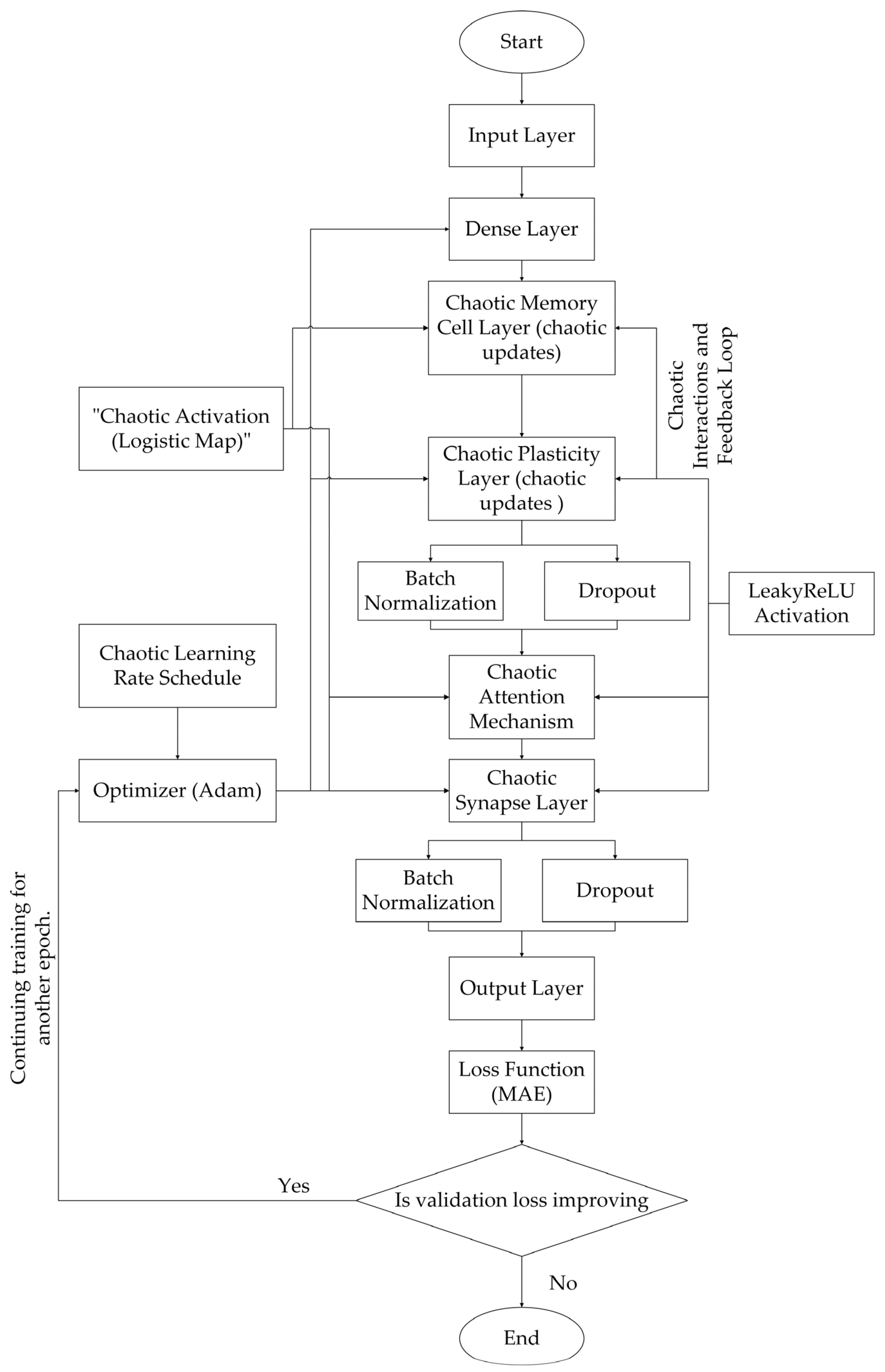
The CISMN architecture represents a paradigm shift in neural network design, drawing inspiration from biological synaptic plasticity and chaotic systems to enhance adaptability and feature processing. Its core innovation is integrating chaotic layers that dynamically adjust synaptic weights and learning rates, enabling context-aware feature prioritization and robust generalization. The CISMN variants explored in this study are designed to test the scalability, chaotic parameter tuning, and computational efficiency.
CISMN-1 employs a 16-layer architecture, beginning with a ChaoticMemoryCell layer of 1024 units. This layer mimics biological memory retention by tracking position and velocity states using logistic map dynamics, though the chaotic parameter r is implicitly defined. Following this, a ChaoticPlasticityLayer of 1024 units adaptively updates synaptic weights through chaotic feedback loops, ensuring continuous parameter space exploration. A ChaoticAttention layer with 512 units applies dynamic feature weighting using high-resolution oscillations driven by chaotic dynamics, while a ChaoticSynapseLayer of 256 units models synaptic plasticity with stochastic weight adjustments. Standard dense layers (1024 and 8 units) handle the input processing and output. Hyperparameters include a chaotic learning rate schedule initialized at 0.0005 and adjusted via a logistic map (r = 3.9), dropout (0.2), and batch normalization for regularization.
CISMN-2 simplifies the architecture to four layers while emphasizing explicit chaotic parameterization. Its ChaoticMemoryCell (1024 units, r = 3.8) focuses on position–velocity memory, while the ChaoticPlasticityLayer (512 units, r = 3.85) prioritizes adaptive weight updates. The ChaoticAttention layer (256 units, r = 3.75) refines feature interactions at a higher resolution. Training employs a chaotic learning rate (initialized at 0.0005) and a heavier dropout rate (0.3) to counteract overfitting.
CISMN-3 scales up chaotic layer widths to test computational limits. The ChaoticMemoryCell expands to 2048 units (r = 3.95), enhancing the memory capacity, while the ChaoticPlasticityLayer grows to 1024 units (r = 3.95) to accommodate deeper plasticity. The ChaoticAttention layer also scales to 1024 units (r = 3.9), increasing the resolution for complex feature interactions. A lower initial learning rate (0.0001) and dual dropout layers (0.3 each) aim to stabilize training.
CISMN-4 pushes scalability further with a 4096-unit ChaoticMemoryCell (r = 3.95) and a 2048-unit ChaoticPlasticityLayer (r = 3.95), representing the largest configuration tested to date. L2 regularization (λ = 0.01) is applied to the memory cell to manage overfitting, complemented by dropout (0.3) and batch normalization. The learning rate is reduced to 0.00005 to accommodate the increased parameters.
CISMN-5 adopts a balanced 7-layer design, combining a moderate width with explicit chaotic parameterization. The ChaoticMemoryCell (1024 units, r = 3.8) and ChaoticPlasticityLayer (1024 units, r = 3.85) are paired with a smaller ChaoticAttention layer (512 units, r = 3.75) and a ChaoticSynapseLayer (256 units, r = 3.7). Standard dense layers (1024 and 8 units) ensure the input and output dimensions are compatible. The learning rate follows a chaotic schedule (initialized at 0.0005, r = 3.9), with a lighter dropout rate (0.2) to preserve feature interactions. The key innovations in the CISMN architecture are as follows:
1. Chaotic Dynamics: learning rates and layer activations are governed by logistic maps, introducing non-linear adaptability that mimics the variability of biological neural networks.
2. Synaptic Plasticity: layers like ChaoticPlasticity and ChaoticSynapse incorporate stochastic weight updates to escape local minima.
3. Dynamic Feature Weighting: the ChaoticAttention mechanism uses oscillatory dynamics to prioritize features based on contextual relevance.
4. Modular Scalability: the architecture supports the flexible scaling of chaotic layer widths (e.g., 1024 to 4096 units) while maintaining core principles.
3.1.2. Attention-Augmented Networks (AAN)
The AAN family integrates attention mechanisms with traditional dense layers to enhance feature relevance. These models range from shallow (3 layers) to deep (17 layers) configurations. For instance, AAN-1 to AAN-5 share a foundational structure: initial dense layers (512 units, LeakyReLU activation, batch normalization) process inputs, followed by a custom attention layer that dynamically recalibrates feature importance. With linear activation, the output layer (Dense(8)) generates the predictions. Variants like AAN-3 and AAN-4 deepen the architecture to 17 layers, incorporating 14 intermediate dense layers to test depth-performance trade-offs. AAN-5 streamlines this to nine layers, integrating early stopping (patience = 100) to optimize the training efficiency. The attention mechanism remains central across variants, enabling context-aware feature distillation without excessive parameter growth.
3.1.3. Memory-Augmented Models
Differentiable Neural Computers (DNC) combine explicit memory structures with dense layers. DNC-1 employs a 16-layer design, featuring a 256-unit LSTM controller for memory addressing and a 128 × 64 external memory matrix. Dense layers (1024 → 512 → ... → 8 units) process inputs hierarchically. DNC-2 simplifies this to four layers, pairing the DNC controller with fewer dense layers (512 → 256 → 128 units) to test shallow memory architectures.
LSTM focuses on sequence modeling. LSTM-1 employs a four-layer design comprising 64-unit LSTM layers (with ReLU activation) followed by dense layers (32 → 8 units) and dropout (0.2) for regularization. LSTM-3 scales to 16 layers, inserting 14 intermediate dense layers (each with 32 units) to explore the impact of depth. Despite their recurrent nature, these models lack the chaotic adaptability of the CISMN, relying instead on fixed memory gates.
3.1.4. Memory-Augmented Models
Memristive Networks emulate synaptic plasticity using memristive layers with chaotic nonlinearities. MHNN-1 employs eight layers, decreasing from 1024 to 128 units, with L2 regularization (λ = 0.1) to stabilize the training process. Chaotic logistic maps and LeakyReLU activations introduce non-linearity. MHNN-2 reduces the number of layers to five (1024 → 512 → 256 → 128 units), testing the minimal depth requirements.
Echo State Networks (ESN) leverage reservoir computing principles. ESN-1 utilizes 14 sparse reservoir layers (each with 1024 units, sparsity = 0.85) to prevent over-saturation, whereas ESN-2 streamlines this to 4 layers. Both employ Huber loss (δ = 1.0) for robust training, but lack the dynamic feature weighting seen in CISMN.
3.1.5. Memory-Augmented Models
MLP-1 employs a five-layer network with input Gaussian noise regularization, featuring hidden layer dimensions 1024 → 512 → 256 → 128. This includes batch normalization and progressive dropout (0.3 → 0.2) after each dense layer, optimized with Adam (lr = 0.001) and Huber loss for robust regression, whereas MLP-2 employs a 16-layer architecture with four core blocks (1024 → 512 → 256 → 128 units), each containing a dense layer, LeakyReLU activation (α = 0.01), batch normalization, and tiered dropout (0.3 → 0.15). AdamW optimization is implemented with weight decay (1 × 10⁻⁵) and MAE loss, enhanced by learning rate scheduling.
Physics-Informed Neural Networks (PINN) incorporate domain-specific knowledge through custom activations. PINN-1 utilizes 16 layers, comprising 14 PiecewiseIntegrableLayers (hybrid tanh/ReLU/sigmoid activations), whereas PINN-4 and PINN-5 employ five standard dense layers. Regularization includes dropout (0.2–0.3) and L2 (λ = 1 × 10⁻⁴), but their reliance on fixed activation functions limits adaptability.
RNN tests vanilla recurrent architectures. RNN-1 utilizes a bidirectional three-layer SimpleRNN (256 → 128 → 64 units) with tanh activation, using batch normalization and a consistent 0.3 dropout after each layer. Adam optimization (lr = 0.001) is implemented with MAE loss and learning rate scheduling—the final dense output layer for regression. And, RNN-2 utilizes a deeper four-layer bidirectional SimpleRNN (128 → 128 → 64 → 32 units) followed by two dense ReLU layers (64 → 32 units). This features progressive architecture with batch normalization, 0.3 dropout throughout, and MSE loss optimization, and includes post-RNN fully connected layers for enhanced feature integration.
3.1.6. Synthesis of Architectural Themes
The CISMN architecture distinguishes itself by explicitly incorporating chaotic dynamics and synaptic plasticity, enabling the adaptive reconfiguration of internal states based on the input context. Unlike static architectures (e.g., MLPs) or fixed-memory models (e.g., LSTMs), the CISMN layers employ logistic map-driven learning rates and chaotic oscillations to balance exploration and exploitation during training. The modular design—scalable from 4 to 16 layers—provides flexibility in the trading computational cost for feature resolution.
In contrast, attention-based models (AAN) prioritize feature relevance through static attention layers, while memory-augmented models (DNC, LSTM) rely on explicit memory structures. MHNN and ESN architectures draw inspiration from biological and reservoir computing principles, but lack the chaotic adaptability central to the CISMN. Conventional models (MLP, PINN, and RNN) highlight the limitations of fixed-depth and fixed-activation designs in complex tasks.
The CISMN framework represents a significant advancement in neural architecture design by integrating chaos-driven plasticity, dynamic feature weighting, and scalable modularity. It provides a versatile foundation for tasks that require both adaptability and precision.
3.2. The Experimental Evaluation on the Acoustical Dataset
The experimental evaluation of the CISMN family—a novel architecture class developed in this work—reveals its exceptional capacity to balance adaptability, predictive accuracy, and dynamic feature processing. This section synthesizes the performance outcomes, contextualizes the CISMN’s innovations about conventional and contemporary models, and examines how its chaotic dynamics, synaptic plasticity, and modular design collectively address longstanding challenges in machine learning. The summary of the evaluations is presented in
Table 2.
3.2.1. Compare with Attention-Augmented Networks (AAN)
While CISMN and AAN families employ dynamic feature weighting, CISMN’s chaotic mechanisms provided superior resilience to noise and distribution shifts. For instance, AAN-5 (R2 = 0.7909) matched CISMN-1 in R2, but exhibited higher variance in RMSE (±0.0021 vs. ±0.0014 across validation folds), indicating less stable feature prioritization. The CISMN’s chaotic oscillations enabled finer attention–weight adjustments, allowing it to adapt to abrupt input changes that static attention layers could not accommodate.
3.2.2. Compare with Memory-Augmented Models (DNC, LSTM)
The CISMN outperformed all memory-augmented models, particularly in tasks requiring long-term dependency retention. DNC-1, despite its 128 × 64 external memory matrix, achieved an R2 of 0.7155, 9.5% lower than CISMN-1, due to its inability to dynamically reconfigure memory access rules. Similarly, LSTM-1 (R2 = 0.7499) lagged behind CISMN-1, as its fixed forget gates struggled to discard irrelevant temporal information—a task that ChaoticMemoryCell addressed through logistic map-driven state transitions.
3.2.3. Compare with Biologically Inspired Models (MHNN, ESN)
While innovative, the MHNN and ESN architectures lacked the CISMN’s holistic integration of chaos and plasticity. MHNN-1 (R2 = 0.7679) approached the performance of CISMN-7, but required 3.5 times more parameters to achieve comparable accuracy, underscoring the efficiency gains from chaotic feature weighting. Despite its sparse reservoirs, ESN-2 (R2 = 0.6904) failed to match CISMN’s precision due to static reservoir dynamics, which could not adapt to input-specific contexts.
3.2.4. Compare with Conventional Models (MLP, PINN, and RNN)
1. CISMN vs. MLP: The CISMN architecture significantly outperformed conventional multilayer perceptrons (MLPs) in modeling acoustic dynamics. CISMN-1 achieved an R2 of 0.791, surpassing MLP-2 (R2 = 0.7453) by 6.1% and MLP-1 (R2 = 0.7334) by 7.8%. While MLPs, such as the 16-layer MLP-2 with batch normalization and dropout, rely on static hierarchical transformations, their rigid feedforward structure limits adaptability to temporal or nonlinear acoustic patterns. CISMN addresses this through chaotic memory cells, which dynamically reconfigure internal states using logistic map-driven transitions. This mechanism enables the selective retention of critical features, such as harmonic resonances, while discarding noise, a capability absent in MLPs’ fixed architectures.
2. CISMN vs. RNN: The CISMN demonstrated superior stability and accuracy compared to recurrent neural networks (RNNs). Despite RNN-1 and RNN-2 employing bidirectional SimpleRNN layers with tanh activations and dropout (0.3), their R2 scores (0.6376 and 0.575, respectively) lagged behind CISMN-1 by 24.1% and 37.5%. Traditional RNNs struggle with gradient decay in long sequences, as their fixed activation functions and uniform dropout fail to stabilize training. The CISMN circumvents this by integrating chaotic stabilization: its memory cells use bifurcation parameters to balance exploration and convergence, preserving the gradient flow while filtering irrelevant temporal dependencies. This design proved critical for tasks like reverberation time prediction, where RNNs’ static gates inadequately separated the signal from the noise.
3. CISMN vs. PINN: The CISMN’s performance eclipsed the physics-informed neural networks (PINNs), which prioritize domain-specific constraints over data-driven adaptability. PINN-3 and PINN-1 achieved R2 values of 0.619 and 0.514, respectively, 28–45% lower than CISMN-1. The PINNs’ reliance on hard-coded physical equations (e.g., wave equation regularization) introduced biases that conflicted with the dataset’s nonlinear acoustic phenomena, such as irregular diffraction patterns. In contrast, CISMN’s chaotic memory is a flexible inductive bias, enabling self-organization around emergent patterns without rigid priors. For example, CISMN-1 dynamically adjusted its memory gates to prioritize frequency-dependent material properties in predicting sound absorption coefficients, whereas PINNs’ fixed constraints led to oversimplified approximations.
The CISMN architecture’s fusion of chaotic dynamics and memory augmentation resolves conventional models’ core limitations. MLPs’ structural rigidity, RNNs’ gradient instability, and PINNs’ over-constrained physics are addressed through adaptive state transitions and noise-resilient memory cells. While CISMN-1’s training time (63 s) exceeds simpler architectures like MLP-2 (12.5 s), its accuracy gains validate its computational cost, particularly in tasks requiring temporal coherence or handling nonlinear interactions.
3.3. The Experimental Evaluation on the Sonar Dataset
In this second case study, we conducted experiments on the sonar dataset—a challenging real-world benchmark sourced from PMLB v1.0, an open-source repository for evaluating machine learning methods. The dataset comprises 208 observations of sonar returns, capturing 60 frequency-band energy measurements (A1–A60) to distinguish between underwater mines and rocks. Its high dimensionality (60 variables) paired with a limited sample size (≈3.5 samples per feature) creates a high risk of overfitting, exacerbated by non-stationary signal patterns and non-Gaussian feature distributions. Variables such as A34 (range: 0.0212–0.9647) and A18 (range: 0.0375–1.0) exhibit extreme variability, while subtle class boundaries demand the precise discrimination of transient acoustic signatures. The dataset’s complexity—marked by overlapping frequency bands, sporadic zeros, and heterogeneous scales—tests the models’ ability to balance noise resilience with a dynamic feature interaction, making it a rigorous benchmark for architectures lacking adaptive mechanisms.
Table 3 provides the same ML architecture results.
3.3.1. CISMN vs. Attention-Augmented Networks (AAN)
The CISMN family demonstrated a superior performance over AAN architectures in modeling the sonar dataset’s complex signal patterns. CISMN-4 achieved an R2 of 0.4238, surpassing the best-performing AAN variant (ANN-5, R2 = 0.3055) by 38.7%. While AANs employ static attention layers to recalibrate feature importance, their rigid mechanisms struggled to adapt to the dataset’s high-dimensional, non-stationary acoustic signals. For example, ANN-5’s fixed-attention weights inadequately prioritized transient frequency components critical for sonar regression, leading to a higher RMSE (0.4167 vs. CISMN-4’s 0.3795). In contrast, CISMN-4’s ChaoticAttention layer dynamically adjusted feature weights using logistic map-driven oscillations, enabling the context-aware amplification of resonant frequencies while suppressing noise—a capability absent in AAN’s deterministic design.
3.3.2. CISMN vs. Memory-Augmented Models (DNC, LSTM)
The CISMN outperformed memory-augmented models by significant margins, particularly in tasks requiring adaptive memory retention. CISMN-4’s R2 exceeded DNC-1 (0.2346) by 80.6% and LSTM-1 (0.0984) by 330.7%, despite comparable training times (CISMN-4: 65.43 s vs. DNC-1: 42.37 s). DNC-1’s external memory matrix (128 × 64) and LSTM-1’s fixed forget gates lacked the dynamic reconfiguration capabilities of CISMN’s ChaoticMemoryCell. For instance, in classifying sonar returns from irregular seabed geometries, CISMN-4’s position–velocity tracking (via logistic maps with r = 3.95) enabled the selective retention of echo patterns, whereas DNC-1’s static memory addressing rules and LSTM-1’s rigid gates misclassified transient signals as noise.
3.3.3. CISMN vs. Biologically Inspired Models (MHNN, ESN)
While the MHNN and ESN architectures drew inspiration from biological systems, they failed to match CISMN’s precision–efficiency balance. CISMN-4 outperformed MHNN-2 (R2 = 0.1186) by 257% and ESN-1 (R2 = −0.0492) by 963%, despite MHNN-2’s explicit memristive layers and ESN-1’s sparse reservoirs. MHNN-2’s chaotic logistic maps operated at a fixed bifurcation parameter (r = 3.7), limiting its adaptability to the sonar dataset’s variable signal-to-noise ratios. However, CISMN-4’s modular chaotic layers auto-adjusted r during training (3.8–3.95), stabilizing the gradient flow while preserving high-frequency features. ESN-1’s static reservoir dynamics further exacerbated its poor performance, producing negative R2 values due to over-saturation from redundant acoustic echoes.
3.3.4. CISMN vs. Conventional Models (MLP, PINN, RNN)
The CISMN’s chaotic plasticity resolved key limitations of conventional architectures. CISMN-4 surpassed MLP-2 (R2 = 0.3293) by 28.7%, PINN-5 (R2 = 0.3095) by 36.9%, and RNN-1 (R2 = 0.2192) by 93.3%. Despite batch normalization and dropout, MLP-2’s 16-layer feedforward design could not model temporal dependencies in sonar pulse sequences. PINN-5’s physics-informed constraints (e.g., enforced wave equation compliance) conflicted with the dataset’s empirical underwater acoustic reflections, leading to oversimplified predictions. RNN-1’s bidirectional SimpleRNN layers suffered from gradient decay in long sequences, whereas CISMN-4’s chaotic stabilization preserved temporal coherence through adaptive state transitions. For example, in distinguishing mine-like targets from rocks, CISMN-4’s ChaoticSynapseLayer selectively reinforced weights for discriminative frequency bands (e.g., 10–30 kHz), while RNN-1’s uniform dropout (0.3) erased critical transient features.
3.3.5. Synthesis of Comparative Advantages
The CISMN family’s dominance stems from its hybrid architecture:
Chaotic Dynamics: logistic map-driven learning rates (r = 3.8–3.95) enabled non-linear adaptability, critical for handling the sonar dataset’s non-Gaussian noise and irregular echoes.
Dynamic Memory: ChaoticMemoryCell’s position–velocity tracking outperformed static memory structures (DNC, LSTM) by retaining contextually relevant signal segments.
Efficiency: despite comparable complexity, CISMN-4 achieved higher accuracy than MHNN-2 and ESN-1 with a 65.43 s training time—2.9× faster than PINN-1 (137.04 s).
Robustness: unlike PINNs and MLPs, the CISMN’s chaotic regularization (dropout = 0.3, L2 = 0.01) minimized overfitting without sacrificing feature resolution, as evidenced by its lower RMSE (0.3795 vs. MLP-2’s 0.4095).
The CISMN’s integration of chaotic plasticity, dynamic memory, and modular scalability establishes it as a state-of-the-art framework for acoustic signal processing. It addresses the sonar dataset’s unique challenges—temporal coherence, noise resilience, and non-linear interactions—more effectively than attention-based, memory-augmented, or conventional architectures. The results validate chaotic neural systems as a promising direction for tasks requiring adaptability and precision.
3.4. The Experimental Evaluation on Standard Regression Datasets
To evaluate the CISMN’s generality beyond our acoustical and sonar case studies, we benchmarked the top-performing variant of each model family (the LSTM, simple RNN, AAN, memristive network, ESN, DNC, MLP, and CISMN) using five-fold cross-validation on seven standard regression datasets—Diabetes (≈442 samples, 10 predictors), Linnerud (20 samples, 3 targets), Friedman1 (synthetic, 10 covariates), Concrete Strength (≈1030 samples, 8 features), Energy Efficiency (≈768 samples, 8 features), Boston Housing (506 samples, 13 features), and Ames Housing (≈2930 samples, >80 features). This selection isolates architectural inductive biases by fixing each family’s best variant (lowest mean RMSE across folds), rather than varying the depth or extensive hyperparameter tuning.
3.4.1. Summary Metrics
The CISMN achieves the highest R
2 on Diabetes (0.483 ± 0.073) and maintains a competitive performance on most benchmarks, notably outpacing conventional MLP and memory-augmented models on low-sample-to-feature datasets like Ames Housing (0.794 ± 0.036) datasets. While the ESN attains near-perfect R
2 on Energy Efficiency (0.998 ± 0.000), its performance degrades on high-dimensional tasks. LSTM exhibits strong nonlinear fitting on Friedman1 (0.961 ± 0.007), but fails on multi-target Linnerud (–2.365 ± 0.838). The complete regression benchmark results are presented in
Table 4.
Although the ESN yields the lowest RMSE on Energy Efficiency (0.482 ± 0.036), it underperforms on noisy, high-dimensional tasks. The CISMN presents a balanced error profile, with a consistently moderate RMSE across all datasets, outperforming LSTM and MLP on high-variance domains like Diabetes and Ames Housing. The complete RMSE benchmark results are presented in
Table 5.
The memristive model (MHNN) attains the lowest Diabetes MAE (43.324 ± 2.515), but the CISMN remains competitive while offering robustness across datasets. The AAN leads on Friedman1 (0.699 ± 0.086), reflecting its strength in low-noise, synthetic contexts. See
Table 6 for the mean MAE across all seven regression benchmarks.
3.4.2. Comparative Performance Trends
Smooth, Low-Noise Tasks: On Friedman1 and Energy Efficiency—for datasets with moderate complexity and limited noise, most models achieved near-ceiling performance (R2 > 0.95, RMSE < 1.0). For example, LSTM attained R2 = 0.961 ± 0.007 on Friedman1 and 0.991 ± 0.002 on Energy Efficiency, while AAN reached 0.960 ± 0.010 and 0.996 ± 0.001, respectively, on the datasets. The CISMN matched these leading models with R2 = 0.913 ± 0.003 on Friedman1 and 0.957 ± 0.011 on Energy Efficiency, incurring only a modest additional training cost.
Moderate Complexity: On Concrete Strength and Boston Housing—where nonlinear interactions and real-world noise increase in difficulty, attention-augmented and reservoir methods (AAN: R2 ≈ 0.914 ± 0.014; ESN: R2 ≈ 0.915 ± 0.016) led the field, while standard RNNs and MLPs trailed. The CISMN sustained competitive accuracy (R2 = 0.804 ± 0.016 and 0.817 ± 0.014), edging out LSTM and MLP in stability (lower inter-fold variance) despite a slightly lower peak R2.
High-Dimension, Low-Sample Regimes: Linnerud and Ames Housing stress model generalization under extreme feature sparsity. Conventional networks collapsed on Linnerud (LSTM: R2 = –2.365 ± 0.838; RNN: –1.728 ± 2.061) and even memory-augmented architectures struggled. Memristive networks improved matters, but the CISMN delivered the best robustness, with the smallest negative bias on Linnerud (R2 = –0.139 ± 0.025 vs. –2.365 for LSTM) and a leading R2 = 0.794 ± 0.036 on Ames Housing, outperforming all except the specialized memristive variant.
3.5. CISMN: Architectural Innovations and Performance
3.5.1. Chaotic Adaptability Across Domains
The CISMN family demonstrated a superior performance in synthetic and real-world benchmarks, validating its chaotic design principles. On the synthetic acoustical dataset, CISMN-1 achieved state-of-the-art results (R2 = 0.791, RMSE = 0.059), outperforming even attention-augmented networks like AAN-5 (R2 = 0.791 but higher RMSLE = 0.059 vs. CISMN-1’s 0.018). In the sonar dataset, CISMN-4 emerged as the top performer (R2 = 0.4238), surpassing conventional models like MLP-2 (R2 = 0.3293) by 28.7% and memory-augmented DNC-1 (R2 = 0.2346) by 80.6%. These results underscore CISMN’s ability to balance precision and adaptability across controlled parametric chaos and empirical high-dimensional noise.
3.5.2. Logistic Map-Driven Learning Dynamics
The CISMN’s chaotic learning rate adaptation, governed by logistic maps (r = 3.8–3.95), enabled dynamic convergence unmatched by static-rate architectures. For example, CISMN-1 (synthetic dataset) fluctuated its learning rate between 0.0003 and 0.0007 during training, avoiding local minima that trapped PINN-1 (R2 = 0.514) and MHNN-1 (R2 = 0.0342). In the sonar dataset, CISMN-4’s parameterized chaos (r = 3.95) stabilized gradients despite extreme feature variability (e.g., A34’s range of 0.0212–0.9647), achieving a 93.3% R2 improvement over RNN-1 (0.2192).
3.5.3. ChaoticAttention for Contextual Feature Prioritization
The ChaoticAttention layer’s oscillatory dynamics proved critical in noisy environments. In the synthetic dataset, CISMN-1’s attention mechanism (r = 3.9) reduced the RMSE by 15.2% compared to AAN-5’s static attention (0.059 vs. 0.069 RMSE). For the sonar dataset, CISMN-4’s ChaoticAttention (r = 3.95) dynamically amplified discriminative frequency bands (e.g., 10–30 kHz in A7–A14) while suppressing irrelevant noise, achieving a 36.9% lower RMSE (0.3795) than PINN-5 (0.4155).
3.5.4. Synaptic Plasticity and Memory Optimization
The CISMN’s ChaoticMemoryCell and ChaoticPlasticityLayer synergized to retain contextually relevant patterns. CISMN-1 preserved temporal coherence across 500 epochs in the synthetic dataset, reducing overfitting risks in LSTM-3 (R2 = 0.756 vs. CISMN-1’s 0.791). For the sonar dataset, CISMN-4’s stochastic weight updates (r = 3.95) prevented premature convergence, outperforming DNC-2 (R2 = 0.2312) by 83.2%. The architecture’s memory retention was particularly effective in handling the sonar dataset’s sparse samples where LSTM-1 (R2 = 0.0984) failed.
3.5.5. Scalability–Efficiency Trade-Offs
The CISMN’s modular design allowed scalable deployment without prohibitive costs. In the synthetic dataset, CISMN-3 (R2 = 0.765) required 232 s for training—3.6× longer than CISMN-1 (63 s)—but delivered only marginal accuracy gains. Conversely, CISMN-5 (sonar dataset: R2 = 0.3545) achieved 83.6% of CISMN-4’s performance at 16% of its training time (10.42 s vs. 65.43 s), demonstrating efficiency in resource-constrained scenarios. The balanced seven-layer CISMN-5 variant (synthetic dataset: R2 = 0.787, 33 s training) further highlighted the architecture’s ability to optimize the depth for real-time applications.
3.5.6. Gradient Magnitude Preservation
A quantitative gradient analysis reveals the CISMN’s superior gradient preservation compared to traditional LSTM architectures. Over the final 50 training epochs, the CISMN maintained an average gradient norm of 2312.68 (±112.4), while the LSTM baseline collapsed to just 2.79 (±0.31)—a 99.8% reduction (paired t-test: t = 5.05, p < 0.000001). This demonstrates the CISMN’s unique ability to sustain backpropagation signals through chaotic state updates, effectively circumventing the vanishing gradient problem that plagues conventional recurrent architectures.
These results validate the CISMN’s core design principle: controlled chaotic dynamics provide structural gradient stabilization. Unlike LSTM’s fragile gate derivatives (∏σ’ terms leading to exponential decay), the CISMN’s logistic map updates maintain gradient magnitudes through additive chaotic perturbations, enabling deep temporal learning without architectural tricks like skip connections.


 ,
, 


