1. Introduction
Decision support systems (DSS) have been incorporated into various domains that require critical decision-making, such as healthcare, criminal justice, and finance [
1,
2,
3,
4,
5]. DSS with explainable artificial intelligence (XAI) assist decision-makers by generating a high-level summary of models/datasets or clear explanations of suggested decisions. This paper examines a challenge encountered by DSS in the domain of credit evaluation: how to deliver accurate and credible summary–explanations (SE). An SE is defined as a local explanation rule
with global information. The following is an example of A globally consistent SE for an observation instance of the Home Equity Line of Credit (HELOC) dataset used in the FICO explainability challenge [
6]: “For all the 100 people with ExternalRiskEstimate
and AverageMinFile
, the model predicts a high risk of default”. An SE rule
being globally consistent means that
y is true for all instances in the support set (the 100 people that satisfy the conditions). Therefore, although SE is specific to a target observation
, it offers a valuable global perspective on the dataset or model.
In credit evaluation, the problem of maximizing support with global consistency (MSGC) aims to deliver a persuasive explanation for the credit evaluation decision by searching for the conditions that are satisfied by both the applicant and most other people in the database (thus maximum support). The MSGC problem can be formulated as an integer programming (IP) problem [
7] and solved by branch-and-bound (B&B) solvers [
8].
Well-supported explanations are convincing, which foster trust in the system among users. Nonetheless, owing to the global consistency constraint, solving the MSGC problem on large datasets often leads to rules that are either highly complex, have low support, or are even infeasible. For many real-world scenarios, explanations with strong support significantly influence user acceptance, whereas minor inconsistencies can often be tolerated. Guided by this observation, this paper addresses the problem of maximizing support with q-consistency (MSqC), , which substantially enhances the support of the SE rule. Consider, for example, a 0.85-consistent SE rule with a support value of 2000: “In over 85% of the 2000 people with ExternalRiskEstimate and AverageMinFile , the model predicts a high risk of default”.
Although the extension seems straightforward, it turns out that the MSqC problem is much more complex than the original MSGC problem. The primary cause lies in the fact that when maximizing the q consistent support, which allows for a proportion of up to of the matched observations to be inconsistent, it is necessary to incorporate all observations with outcomes different from the target into the MSqC formulation. This requirement, i.e., the inclusion of outcome-divergent observations, was absent in the original MSGC problem.
Besides formulating the MSqC problem, this paper also addresses the following challenges:
- 1.
Efficiently solving the MSqC problem with large datasets. The B&B method is inefficient on IP problems with large datasets, including MSGC and MSqC. For example, a 60-second time limit should be established to terminate the solution [
7]. In our reproduction, solving MSGC with the SCIP solver [
9] requires 1852 s for
K and 101 s on average for datasets of size
K. As demonstrated by the experimental results, the performance of the B&B method degrades significantly when solving the more complex MSqC problem. Therefore, a more efficient and scalable solver is needed to solve the MSqC problems on a large dataset.
- 2.
Finding explanations that extrapolate well. In certain domains, such as credit evaluations, optimization models are often addressed within a subset of the global data, owing to practical considerations including transmission efficiency, privacy protection, and distributed storage solutions. Therefore, explanations with high support and consistency on a local dataset should also exhibit these qualities on the global dataset. This extrapolation effectiveness of explanations should be measured, and the explanations obtained by our method should exhibit good extrapolation effectiveness.
The primary contributions of this study are summarized below:
- 1.
The MSqC problem is novelly formulated for the first time, which can generate structured explanations (SEs) with substantially higher support, achieved by allowing for slight reductions in consistency.
- 2.
The simplified increased support (SIS)-based WCS method is proposed for solving the MSqC problem efficiently, which is much more scalable than the standard B&B method.
- 3.
A global prior injection technique is proposed to further improve the SIS-based WCS method for finding SE with better extrapolation effectiveness.
This paper is organized as follows.
Section 2 introduces the background and related studies.
Section 3 formally defines the globally consistent SE and
q-consistent SE, and formulates the MSGC and MSqC problems. Then,
Section 4 introduces the proposed SIS-based WCS method and the global prior injection technique. In
Section 5, computer experiments are conducted to evaluate the effectiveness of the proposed methods, in terms of both the solving time and solution quality. Finally,
Section 6 concludes the paper.
2. Background
2.1. Explainable Artificial Intelligence
Explainable Artificial Intelligence (XAI) refers to a collection of techniques and methods aimed at making AI models more transparent and understandable to human users. Traditional black-box machine learning models, such as deep neural networks and ensemble methods, often yield high predictive accuracy but lack interpretability, making it difficult for users to trust and adopt their decisions in critical applications [
10]. XAI seeks to bridge this gap by providing insights into model behavior, offering explanations that enhance accountability, regulatory compliance, and user trust [
11,
12,
13].
XAI methods can be broadly classified into intrinsic interpretability and post hoc interpretability [
11]. Intrinsic methods involve models that are inherently interpretable, such as decision trees, linear regression, and rule-based models. These models provide transparency by design, allowing users to trace decision pathways directly.
Post hoc interpretability, on the other hand, involves techniques applied after training a complex black-box model. These include feature importance analysis, local interpretable model-agnostic explanations (LIME) [
14], and Shapley additive explanations (SHAP) [
15]. Post hoc methods can provide global (explaining the overall behavior of a model) or local (explaining a specific decision) insights into model predictions.
Despite significant progress, XAI faces multiple challenges. For example, (1) simpler models are often more interpretable but may lack predictive power [
16] (accuracy vs. interpretability trade-off); (2) many XAI methods are computationally expensive and struggle to scale [
17] (scalability and efficiency); (3) XAI methods can be susceptible to adversarial manipulations [
18] (robustness against adversarial attacks); (4) integrating XAI tools into existing systems often require specialized knowledge [
11]. Recent studies have also emphasized the value of incorporating diverse contextual factors to enhance interpretability in complex domains, such as travel demand prediction using environmental and socioeconomic variables [
19].
2.2. Combinatorial Optimization in XAI
Combinatorial optimization involves mathematical techniques for selecting the optimal solution from a finite set of possibilities. Common approaches include Mixed-Integer Linear Programming (MILP), Constraint Programming (CP), heuristic search, and branch-and-bound methods [
20]. These techniques have found applications in enhancing XAI by providing rigorous ways to enforce transparency constraints and ensure optimal interpretability [
16].
Feature Selection and Dimensionality Reduction: Combinatorial optimization can be used to identify the smallest subset of features that maintain model performance while improving interpretability. MILP-based feature selection methods have been shown to enhance transparency by reducing unnecessary complexity [
18].
Optimized Decision Trees and Rule Lists: Recent studies have demonstrated the use of combinatorial optimization for training globally optimal decision trees and rule-based models. These methods directly optimize for both accuracy and interpretability by minimizing tree depth or the number of decision rules [
16,
21,
22,
23,
24].
Counterfactual Explanations: Counterfactual explanations provide actionable insights by showing the minimal changes required for a different model outcome. The generation of optimal counterfactual examples is a combinatorial problem that can be effectively solved using MILP [
25].
2.3. Enhancing Credit Evaluation with Combinatorial Optimization
Financial decision-making, particularly in credit evaluation, relies heavily on machine learning models. Regulatory requirements such as the General Data Protection Regulation (GDPR) mandate transparency in automated decision-making, requiring lenders to provide clear explanations for loan approvals and rejections [
26].
The use of combinatorial optimization techniques in credit evaluation systems has proven beneficial in several key areas.
Monotonic Constraints in Credit Scoring: First, monotonic constraints in credit scoring ensure that model outputs remain aligned with financial intuition. For instance, increasing a borrower’s income should not decrease their creditworthiness. These constraints can be effectively enforced using MILP, allowing models to maintain both interpretability and regulatory compliance [
27].
Optimal Credit Scoring Models: Second, combinatorial optimization facilitates the development of optimal credit scoring models. By deriving sparse yet highly predictive models, these techniques enable the creation of interpretable scoring systems that provide transparent creditworthiness assessments while maintaining strong predictive performance [
17].
Counterfactual Explanations for Loan Decisions: Finally, counterfactual explanations generated through MILP provide actionable insights for loan applicants. These explanations suggest specific changes that applicants can make to improve their credit standing, such as reducing outstanding debt or increasing savings. By offering tailored guidance, counterfactual explanations enhance the fairness and transparency of credit decision-making [
28].
The integration of combinatorial optimization into XAI for credit evaluation not only improves model interpretability but also aligns with regulatory standards. Transparent models enable financial institutions to audit decision-making processes, ensuring fairness and reducing bias. Moreover, by providing clear, actionable explanations, these methods help to build trust between customers and lenders, ultimately leading to more responsible AI deployment in financial services [
26].
In some scenarios, no models exist to generate neighborhood data, and the sole source of knowledge is historical or pre-provided data. One prominent instance of this scenario corresponds to the FICO explainable machine learning challenge [
6], in which the FICO company was provided a dataset generated by its black-box model, yet the model itself remained inaccessible to researchers. For situations in which data alone are accessible, and the model itself is not accessible, a more data-centered approach is necessary. Two possible options are to fit a model to the data and provide interpretations of it [
29,
30], or explain the decisions based on data patterns [
7,
31]. For example, globally consistent rule-based summary–explanation (SE) was proposed in [
7], casting the problem of maximizing the number of samples that support the decision rule as a combinatorial optimization problem, called the maximizing support with global consistency (MSGC) problem.
However, the global consistency constraint in MSGC often results in infeasibility or small support for the SE solution of MSGC on many practical large datasets. Indeed, in many real-world scenarios, explanations with high support facilitate users’ trust in the explainer system, whereas minor inconsistencies can often be acceptable within certain thresholds. Guided by this idea, we generalize the MSGC problem to MSqC in this paper by permitting a small inconsistency level q in explanations, thereby significantly enhancing the support of the SE rule.
While our proposed MSqC framework focuses on optimizing the trade-off between support and consistency in rule-based explanations, it also shares conceptual similarities with approximation-based rule generation methods, such as “probably approximately correct” (PAC) rules [
32]. These methods often allow a small fraction of exceptions or errors in order to improve the generalization capacity of learned rules.
However, there are important differences. PAC-style rule learners typically operate in a probabilistic framework, relying on distributional assumptions and statistical learning theory to guarantee generalization. Moreover, many of these methods are model-dependent and aim to learn classification rules applicable across the dataset. In contrast, our MSqC framework is model-agnostic and deterministic, directly optimizing rule support under a user-defined consistency threshold q without requiring any probabilistic assumptions or model access. Furthermore, MSqC generates target-specific summary–explanations that not only maximize support but also ensure interpretability in high-stakes decision-making settings, such as credit evaluation.
This distinction positions MSqC as a novel contribution in the space of interpretable explanation frameworks with a focus on optimization-based control over consistency and coverage rather than statistical generalization guarantees.
3. Problem Formulation
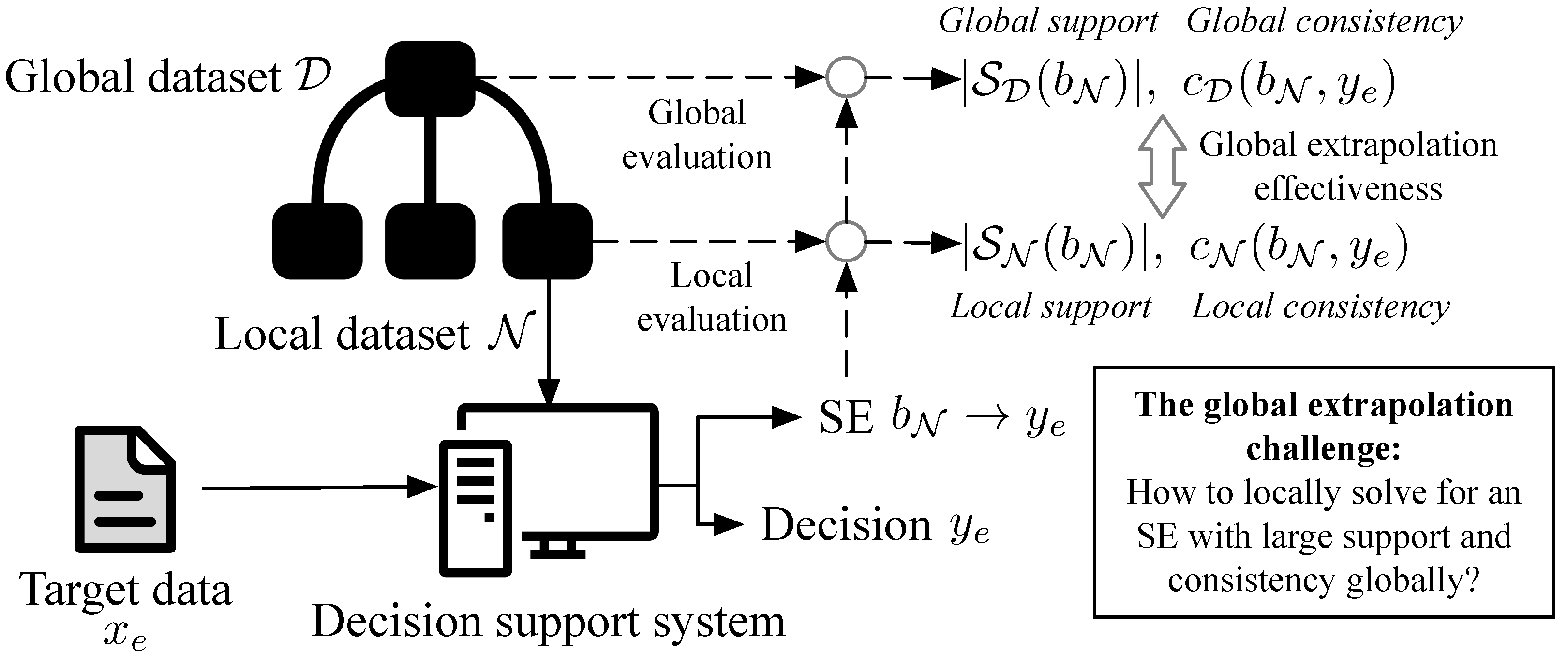
In this section, we first introduce the typical use cases of SE under a credit risk assessment scenario; then, the formal definitions of SE, its max-support problem, the consistency level, and the extrapolation challenge are presented in the rest of this section.
3.1. A Credit Risk Assessment Scenario
Here, a credit risk assessment scenario is used to illustrate the use cases and specific forms of SEs generated through a decision support system (DSS). Given input data
(also called target data, indicating that it is the target to be explained), the DSS outputs a suggested decision
and the SE that explains the target observation
.
Figure 1 illustrates two cases in which the DSS responses to the request of a loaner or a banker, facilitating their comprehension of the target observation
using SEs that reveal the risk levels of the instances in the dataset similar to
.
The figure also shows that different SEs can have varying degrees of impact on users’ trust, depending on its level of credibility. In general, SEs with large support and high consistency levels are more convincing, promoting trust, while SEs with small support or low consistency levels are less persuasive, therefore undermining users’ trust in the system. On the right-hand side of the figure, a comparison is made between the globally consistent SE [
7] and the
q-consistent SE proposed in this paper using a target observation sampled from the 10K-sized FICO dataset [
6]. It can be seen that while the globally consistent SE has a consistency of 100%, it has very small support (which is typically the case for globally consistent SEs). In contrast, the
q-consistent SE attains much greater support at the cost of a lower consistency of 82%, which, given its advantages, should be acceptable for this scenario, as well as potentially for many others.
3.2. Globally Consistent Summary–Explanation
The summary–explanation (SE) is defined on a truth table, i.e., a -dimensional observation dataset with binary features . Further, serves as the index set for observations, while represents the set of indices for binary feature functions. In the credit risk assessment scenario, binary labels are used to denote high (1) or low (0) risk, although it should be noted that SE does not require labels to be binary. In general, such a truth table can be derived from any dataset with arbitrary inputs . As an illustration, the initial input vector is converted into the binary representation , through the ordered feature function set . Henceforth, the terms ’feature’ and ’feature function’ are treated as synonymous.
Let b denote a conjunctive clause constructed by the logical AND (∧) of multiple conditions, where each condition corresponds to a binary feature , i.e., , where represents a subset of the feature set . For the example above, b could be , or .
A summary–explanation (SE) is a rule
that describes the binary classifier
A globally consistent SE for an observation
is an SE
with the following properties:
- 1.
Relevancy, i.e., ;
- 2.
Consistency, i.e., for all observations , if , then .
In a more accessible manner, a globally consistent SE can be articulated as follows: “for every observation (such as people or customers) where the clause holds, the outcomes (e.g., predicted risk/decision) matches the label of observation e”. This type of explanation aligns the current observation with historical data points in the dataset, thereby making it more persuasive to users in domains such as credit evaluation.
The quality of the clause is evaluated using two metrics:
- 1.
Complexity , which is the count of conditions within b;
- 2.
Support , which represents the cardinality of the support set , is defined as the set of observations in that satisfy clause b. Specifically, .
As is customary, the term support can refer to either the support set or its cardinality , depending on the context. To prevent ambiguity, this paper uses set notation to denote either index sets or original sets for notational simplicity.
3.3. Minimizing Complexity and Maximizing Support
The challenges of minimizing complexity with global consistency (MCGC) and maximizing support with global consistency (MSGC) for SE
were introduced by Rudin et al. [
7]. The MCGC problem aims to identify a solution
b that minimizes complexity
, and this objective can be modeled as the following IP model:
where the binary decision variable
signifies that feature
p is included in the resulting clause
, i.e.,
and
otherwise. These variables,
, are termed feature variables. Additionally, the binary variable
signifies whether observation
i satisfies binary feature
p, i.e.,
. The activation feature set
for an observation
e consists of the features that are satisfied by
e, i.e.,
. In addition,
represents the set of consistent observations, defined as
. Therefore, the set of inconsistent observations is
, where for each
, it holds that
. The relevancy property is guaranteed by selecting features from
only, while the consistency property is ensured by condition (
2), which ensures that for any observation with
,
. The solution of the MC model is fast, due to simplicity; however, it does not guarantee large support.
The MSGC problem can be viewed as an extension of the MCGC problem, where the objective is to find
b with maximal support
, subjecting to a complexity constraint
. As indicated by Rudin et al. [
7], this paper adopts
value deemed reasonable for the complexity of SE in credit evaluation. The MSGC problem is formulated as follows:
where the binary decision variable
denotes whether observation
i is included in the support of clause
, i.e.,
if and only if
. Additionally, the constant
M must satisfy
. Equation (6) enforces that for an observation
to be part of
’s support, all conditions within
must be satisfied by
i. While the support of the MSGC SE is typically larger than that of the MCGC SE, solving the MSGC model (
4)–(
8) is notably slower due to its elevated complexity.
3.4. The Third Metric: Consistency Level
Formally, a globally consistent symbolic explanation corresponds to a 1-consistent or 100%-consistent rule, as it mandates perfect consistency across all observations . However, deriving such a strictly consistent rule is often computationally challenging if not outright impossible in real-world datasets. For large-scale applications, both the MCGC and MSGC models typically yield rules with either excessive complexity, insufficient support, or infeasibility. The rationale is straightforward: complex datasets rarely contain 1-consistent rules with moderate complexity (e.g., ) Consequently, relaxing the consistency requirement from strict 1-consistency to a more lenient threshold such as 0.9 or 0.8 becomes a pragmatic choice. This relaxation is widely acceptable in practical SE applications, including credit evaluation, where near-consistent rules often suffice for actionable insights.
We characterize
q-consistency as the following condition: for at least a fraction
q of the samples where
, it holds that
. Define
as the set of consistent examples, i.e.,
. Formally, the consistency measure for the rule
is defined as the ratio of consistent examples to the total support, i.e.,
Consequently, the
q-consistency requirement translates to ensuring that this ratio meets or exceeds
q, i.e.,
.
A
q-consistent SE
for an observation
can be restated as follows: ”For more than
q proportion of all the observations where
holds true, the outcomes are
”. For instance, in the domain of credit evaluation, a
q-consistent SE for an observation of the HELOC dataset [
6] can be as follows: “For over 80% of all the 1108 people with NumTotalTrades
and NumTradesOpeninLast12M
, the model predicts a high risk of default”. From the above, it can be seen that the essence of the summary–explanation lies in the following factors: (1) informing the applicant about how many people share similar features with the applicant (i.e., the support), and (2) explaining to the applicant that among these similar individuals, a q-fraction of them defaulted. As a result, the system provides a credible explanation of why the applicant is classified as high risk and consequently rejected.
Naturally, the problem of maximizing support with
q-consistency (MSqC) can be extended from the MSGC problem (
4)–(8). The objective of MSqC is to maximize the support of SE
while subjecting to the
q-consistency constraint
, which can be formulated as follows:
Compared to the MSGC model (
4)–(8), four modifications are introduced, listed as follows.
- 1.
Binary variables (representing supportive observations) are defined for all observations , rather than just for consistent observations .
- 2.
Constraints (11) now incorporate , allowing for inconsistent support () for . Specifically, recall that in MCGC and MSGC, the consistency constraint requires that for any inconsistent observation i, the SE rule is not satisfied, i.e., . Thus, constraints (2) and (5) in the MCGC and MSGC problems mean that at least one clause p in the SE rule b (i.e., ) needs to be unsatisfied (i.e., . Here, in MSqC, some inconsistent observations may also satisfy the SE rule b. Thus, constraint (11) imposes only on those observations that are not supportive ().
- 3.
Constraints (12) now apply to all instead of only those in , simply because are now defined for all observations , rather than just for consistent observations . As in MSGC, this constraint enforces that for any supportive observations (); it must hold that , i.e., whenever , we have , for i with .
- 4.
Equation (4) introduces the
q-consistency constraint, where binary constants
denotes
. Specifically, since the number of the consistent examples is
, and the size of the support is
, by the definition of the consistency measure
(
9), constraint (14) describes the
q-consistency constraint
.
Remark 1.
Previous research [7] has demonstrated that MCGC and MSGC are NP-hard. The model formulations MCGC (1)–(3), MSGC (4)–(8), and MSqC (10)–(15) reveal a clear progression in their complexity levels. Formally proving the NP-hardness of MSqC is left as future work, but its complexity dominance over MSGC and MCGC is evident from the increased model size, i.e., MSqC has strictly more variables and constraints while maintaining a similar structure. 3.5. The Extrapolation Challenge
In domains such as credit evaluations, optimization models are often solved over a subset of the global data, driven by practical factors such as transmission efficiency, privacy concerns, and distributed storage. As shown in
Figure 2, the DSS optimizes an SE on one of the local datasets, while the SE may be evaluated later on the global dataset. The extrapolation challenge states that if the SEs given by the DSS have large support and consistency locally, then they should also have large support and consistency level if evaluated on the global dataset.
More formally, let denote the global dataset (index set), and be a local dataset (index set) that is drawn randomly from . For a target observation to be explained, an SE rule is sought by solving an optimization problem on . During the solution process, the local support and local consistency level of an SE rule can be computed on the local dataset . However, as the global dataset is inaccessible during the optimization process, the challenge in extrapolation lies in improving the global support and global consistency level without direct access to the global dataset.
4. Methodology
As formulated in the previous section, the generation of an SE can be implemented by solving an optimization model. Specifically, three IP models, i.e., MC, MSGC, and MSqC, have been introduced to optimize the SE for different objectives.
Since we aim to enhance the credibility of SE by increasing its support, our focus is on the solution algorithms for MSGC and MSqC.
The MSGC model [
7] is solved with B&B solvers such as SCIP [
9]. However, the B&B method is hardly applicable on these IP models with large datasets, because not only is B&B an exact solution method, but also MSGC and MSqC are NP-hard. Therefore, it is necessary to develop an approximate solution algorithm for large-scale MSqC problems that is not only efficient but also find SEs that extrapolate well (see
Section 3.5).
However, most approximate algorithms, including evolutionary algorithms (e.g., genetic algorithms and particle swarm optimization) are not suitable for our objective, because both MSGC and MSqC are large combinatorial problems with numerous constraints. Specifically, the MSGC problem has binary decision variables and constraints, and the MSqC problem has binary decision variables and constraints. As a result, regular evolutionary methods struggle to even find a feasible solution for MSGC and MSqC.
Our method is based on a heuristic sampling approach that shares similarities with stochastic optimization methods such as stochastic subgradient descent [
33,
34]. However, unlike purely random sampling, each sub-problem in our framework is constructed in a guided manner using SIS scores, which incorporates global prior knowledge about feature importance (called global prior injection). This guided sampling helps improve the representativeness of selected sub-problems and addresses the extrapolation challenge commonly encountered in local explanation methods.
In this section, we first introduce the the SIS scores-based sampling method for feature variables, then the global prior injection technique that aims to improve the SE solutions quality on the global dataset, and finally the proposed SIS-based WCS optimization algorithm framework. The relationship of the different components in the optimization framework is illustrated in
Figure 3. In short, to achieve scalability in time efficiency, the WCS optimization algorithm decomposes a large MSqC problem into multiple smaller MSGC sub-problems and finds the optimal solution among the solutions of the MSGCs. Each MSGC is obtained by the column (feature) and row (instance) sampling of the dataset
, with column sampling weighted by the features’ pre-computed SIS scores. The global prior injection technique embeds global preferences of the features into their SIS score distribution, utilizing the fact that SIS scores can be computed before the solution process.
For the convenience of the reader, the symbols used throughout this paper are listed in the
Supplementary Materials.
4.1. Simplified Increased Support
The simplified increased support (SIS) is a score of feature variables by which the smaller IP sub-problems (i.e., the smaller MSGCs) determine their selection of variables. In other words, each smaller MSGC problem is generated by sampling (without replacement)
with the number of feature variables from the activation feature set
according to the features’ SIS scores
, which is defined as the follows:
The derivation process is detailed in the
Supplementary Materials. In line with our intuition, this involves weighting a feature
p by the frequency with which it is satisfied by observations where
, subtracting a feature
p by the frequency at which it holds across observations where
. The sampling probability for each feature
p is
with
where
denotes the Softmax function,
s represents the SIS vector defined in (
16),
is the SIS vector normalized and scaled by a factor
a, and
signifies the
pth element of
corresponding to the feature variable
.
4.2. Global Prior Injection
To address the global extrapolation challenge, we propose that global prior information should be incorporated into each WCS IP model’s local solution procedure through
, which is an extension of (
16) as shown below:
where
represents the subset of consistent observations within the global dataset
, specifically defined as
. By defining
, and leveraging the binary nature of
, the complementary sum over inconsistent observations is
. Notably,
and
are exclusively determined by the global dataset
; as such, these values can be pre-computed and applied to multiple summary–explanation queries.
4.3. The Weighted Column Sampling Optimization Framework
The proposed WCS optimization framework for approximately solving the MSqC model (
10)–(15) can be decomposed into formulating, resolving, and integrating the solutions of
number of smaller IPs, each of which is an MSGC model (
4)–(8) with an observations dataset
and feature set
. The overall procedure of the WCS optimization framework is shown in
Figure 3 and Algorithm 1.
To be more specific, let denote the ith sub-problem. The observation dataset for is uniformly randomly sampled (without replacement) with a given size , and the feature set is sampled (without replacement) with a given size from the activation feature set of the original MSqC problem, according to the global-prior-injected SIS-based probability . Given that every problem is not large in scale, they can be solved with the B&B algorithm efficiently. Moreover, since the iterations within the for-loop are independent of each other, parallel processing can be utilized to accelerate the solution process.
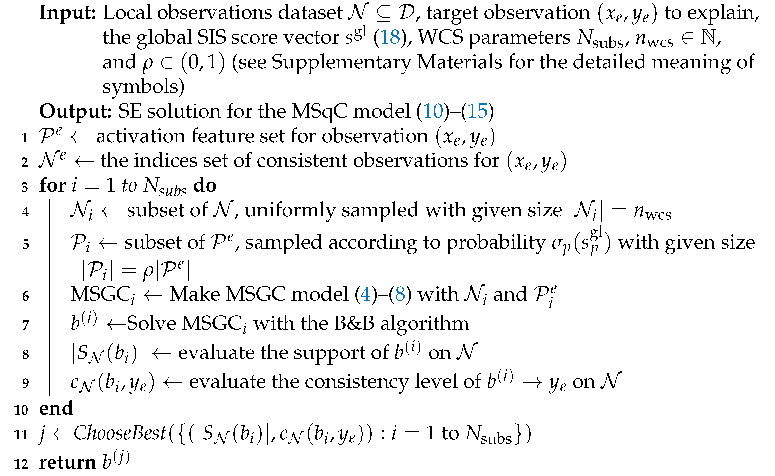
| Algorithm 1: The SIS-based WCS optimization algorithm |
![Mathematics 13 01305 i001]() |
Finally, the ChooseBest function can be implemented in multiple ways. Since both the support and consistency level should be maximized, their product can serve as the sole selection metric, and either one can be given priority. In the case of credit risk assessment, this study employs a method where the solution with the maximum support is searched first among those with a consistency level exceeding 80%. If no such solutions exist, the search continues with those having a consistency level exceeding 75%, and so forth.
The solution time of MSqC(WCS) depends on
, the solution time of each sub-problem
, and the
ChooseBest function. As analyzed by Rudin et al. [
7], each
is NP-hard. However, fixing
and
can set the time complexity of
to a constant level, denoted as
K. The
ChooseBest function is of time complexity
. Then, the time complexity of MSqC(WCS) will be
. The space complexity of MSqC(WCS) is
, where
denotes the number of threads running concurrently. The space complexity of each sub-problem
can also be set to a constant level by fixing
and
; then, the space complexity of MSqC(WCS) will be
. In our experiments, we typically use
,
, and
, and it can be verified in
Section 5 that the solution time of MSqC(WCS) does not increase with the size
of the local solution dataset.
5. Computer Experiments
It is worth noting that our method differs fundamentally from popular model-dependent explanation techniques such as LIME [
14] and SHAP [
15]. These methods aim to interpret the predictions of a trained black-box model by quantifying the contribution of each input feature to the output for individual instances. In contrast, our approach is model-agnostic and dataset-driven: it constructs rule-based summary–explanations that describe subpopulations satisfying certain logical conditions with high support and acceptable consistency, without referencing any specific prediction model.
Due to these fundamental differences in scope and goal, direct empirical comparisons with LIME or SHAP are not meaningful. Instead, we focus on comparing our method against structurally similar summary–explanation models (e.g., MSGC and MSqC solved via B&B) to evaluate performance in terms of support, consistency, and runtime. This comparison better reflects the relative advantages of q-consistent SEs in rule-based, global interpretability contexts.
Specifically, in this section, three different SE generation methods are tested and compared: MSGC(B&B), MSqC(B&B), and MSqC(WCS). The SE generation methods are implemented by solving MSGC or MSqC with the B&B or WCS methods. Note that we have used the notation <Model> (<Method>) to denote solving model <Model> using solution method <Method>. For example, MSqC(WCS) denotes solving MSqC (
10)–(15) with the SIS-based WCS method and using the solution as the SE output (see
Figure 3).
5.1. Experimental Setup
Dataset descriptions. Here, three distinct credit-related datasets are utilized to validate the effectiveness of our approach. The first one is the renowned HELOC dataset, employed in the FICO machine learning explainability challenge [
6]. The other two datasets are sourced from the UCI Machine Learning Repository: Taiwan Credit [
35], focusing on credit card client default cases in Taiwan, and Australian Credit Approval [
36], which concerns credit card applications. In the following, we primarily describe the application of different methods to the HELOC dataset. For detailed information about the Taiwan Credit and Australian Credit Approval datasets, as well as a comparison of the different methods on these three datasets, please refer to
Appendix A.
The HELOC dataset contains the credit evaluation-related information of an individual, such as their credit history, outstanding balances, and delinquency status. The information are stored in 23 feature variables, including numeric and discrete types with missing values. (Note that, in addition to handling missing values, features binarization is required to establish the MSGC and MSqC model, which will generate more binary features than the original dataset.) The target variable “RiskPerformance” represents the repayment status of an individual’s credit account, indicating whether the individual paid their debts as negotiated over a 12–36 month period. The dataset contains data for 10,460 individuals, which is reduced to
after data cleaning. Further details of this dataset are given in the
Supplementary Materials.
Data preprocessing. The dataset used in our experiments has been pre-cleaned and does not contain any missing values. All features are either numerical or categorical. To handle categorical features, we first apply label encoding to convert string values into integers, followed by one-hot encoding to produce binary feature indicators. This representation is compatible with our summary–explanation (SE) framework, which operates on boolean-valued feature functions. For numerical features, we use quantile-based thresholding to generate binary features. Specifically, we select a small number of quantile cut-off points (e.g., quartiles) and transform each numerical variable into a set of binary features indicating whether its value exceeds each threshold. This preprocessing ensures that all features used in the SE models are binary-valued and suitable for logical clause construction.
Distributed storage simulation: To evaluate the global extrapolation effectiveness of the different methods, it is necessary to mimic the distributed storage of datasets and carry out the local solution of MSGC and MSqC models. Here, we use a local–global ratio parameter to control the size of the local dataset . At , it is equivalent to having no distributed storage, and the models are solved directly on the global dataset.
Parameters and hardware:
Table 1 presents the parameter settings employed in the experiments. Experiments were carried out on a Mac Mini desktop featuring an M1 chip.
Metrics: The SE generation methods are evaluated from three different aspects, i.e., solution speed, local solution effectiveness, and global extrapolation effectiveness. Specifically, given a target observation and an SE solution of an SE generation method, five metrics are computed, which can be grouped as follows:
- 1.
Local solution performance metrics, i.e., solution time , local support and local consistency level .
- 2.
Global extrapolation performance metrics, i.e., global support and global consistency level .
As is customary, the metrics are calculated by averaging across multiple algorithm executions using the 1-shifted geometric mean, which exhibits resilience to outliers of all magnitudes [
37].
Experimental Procedure
The experiment consists of the following three phases:
- 1.
Preprocessing phase: The missing values were handled and features were binarized. Specifically, ordinal features are binarized with
quantile thresholds, and categorical features are binarized into one-hot vectors. Then, the global SIS scores
(
18) of features are computed.
- 2.
Execution and parameter sweep phase: In order to investigate how the performance of the three methods are impacted by different parameter configurations, a parameter sweep was conducted. Specifically, for each parameter setting (mainly varying and with other parameters fixed), a round of experiment was conducted, which can be divided into the following two steps.
- (a)
Request scenario generation: A local dataset consisting of observations was sampled from the global dataset, and an explanation request was randomly generated by selecting an observation from the global dataset as the target observation to be explained.
- (b)
Problem formulation and solution: The MSGC and MSqC models were established, and then the MSGC model is solved by B&B and MSqC is solved by both B&B and the proposed SIS-based WCS method. The names of the SE generation methods, i.e., MSGC(B&B), MSqC(B&B), and MSqC(WCS), indicate which model is being solved by which solution method. Metrics were calculated and recorded. This process was repeated times, and then the 1-shifted geometric mean of the metrics was calculated.
- 3.
Results and analysis phase: The results of the experiments were analyzed and discussed.
In the following, we first take a quick look at how the SEs produced by MSqC(WCS) are different from the SEs produced by MSGC(B&B) by sampling a few results from the SE solutions; then, the results are compared in details on local solution effectiveness and global extrapolation effectiveness, respectively. In
Appendix A, the results for two other datasets are also presented.
5.2. Sampled Results of the Summary–Explanation Solutions
For an illustration of the SE solutions in practical applications,
Figure 4 compares several example SEs generated by MSGC(B&B) and MSqC(WCS) methods for random target observations when
. It can be observed that the SEs produced by MSqC(WCS) have much greater support while maintaining consistency within an acceptable range for the credit evaluation scenario.
5.3. Local Solution Effectiveness
The effectiveness of local solutions for various methods is evaluated by contrasting their solution time, local support size, and local consistency scores.
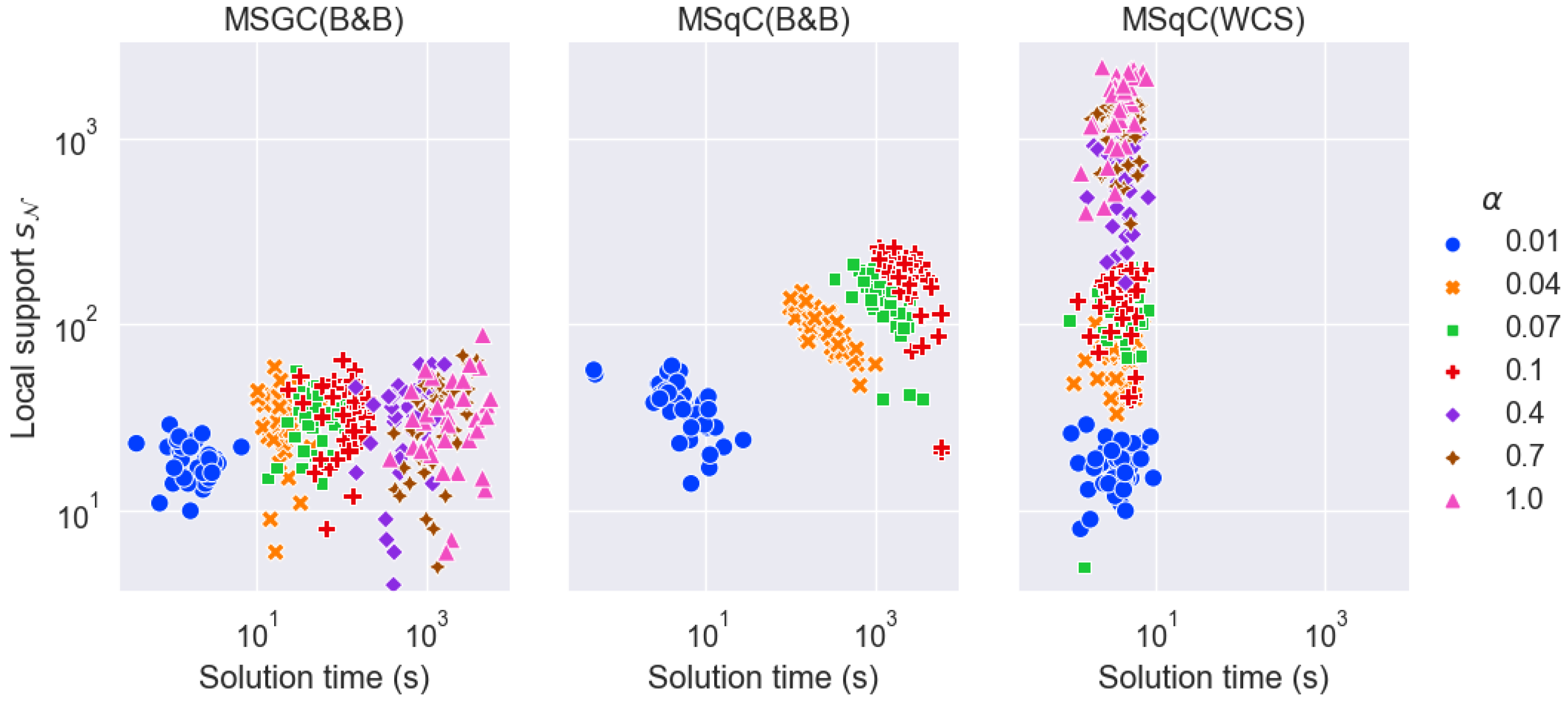
Table 2 shows the local solution performance of the three methods under different settings of the local–global ratio
with WCS sub-problem size
. We have the following observations.
- 1.
Solution time : MSGC(B&B) and MSqC(B&B) scale poorly with respect to the size of the local dataset ( increases drastically as increases from 0.01 to 1, which corresponds to increases from approximately from 0.1 K to 10 K). When K, MSqC(B&B) fails to complete within the 2-h time limit. In contrast, the solution time of MSqC(WCS) is independent of , and in fact, it relies only on the number and complexities of the WCS sub-problems.
- 2.
Local support
: MSGC(B&B) yields SE solutions with the smallest local support, while MSqC(B&B) yields SE solutions with the largest. This is the expected result which motivates the formulation of the MSqC problem (see
Section 3.4). Furthermore, MSqC(WCS) solutions also have much larger local support than MSGC(B&B), though not as large as MSqC(B&B). These observations of the local support and solution time of the different methods are also demonstrated in
Figure 5.
- 3.
Local consistency level : MSGC(B&B) solutions always have a local consistency level of , and MSqC(B&B) solutions always have , because B&B is an exact solution method. Compared with the two B&B-based methods, MSqC(WCS) solutions generally have lower local consistency levels.
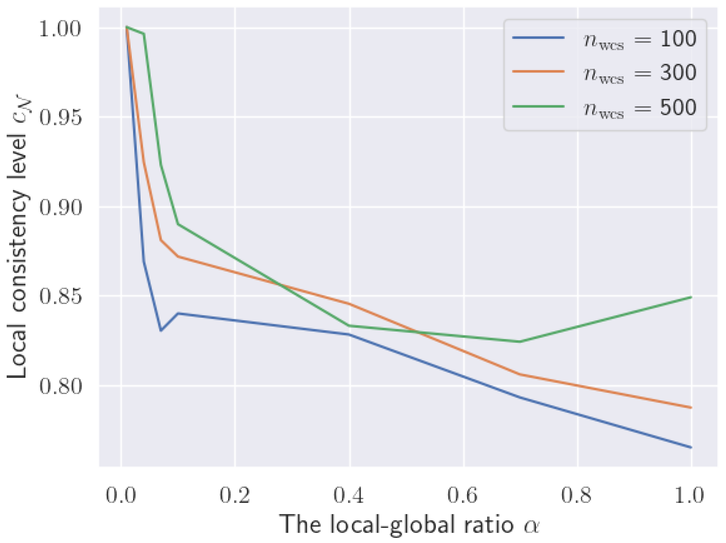
However, the local consistency levels
of the MSqC(WCS) solutions can be raised by increasing the WCS sub-problem size
, as demonstrated in
Figure 6, for most local–global ratio values
. Increasing the sampled feature ratio
can also achieve the same goal, though the experiment is omitted. Note that stochastic variations exist for the performance of MSqC(WCS) because of the randomness in observations and features sampling (see Algorithm 1).
In summary, MSqC(WCS) offers superior time efficiency compared to MSqC(B&B) at the expense of reduced local support and lower local consistency levels . However, the local support is still significantly larger than that of MSGC(B&B), and its local consistency levels remain relatively close to the desired value . Moreover, the local consistency levels of MSqC(WCS) can be further improved by adjusting parameters, although this may increase the solution time, necessitating a trade-off based on the specific situation.
5.4. Global Extrapolation Effectiveness
As highlighted earlier, in real-world scenarios, model solving typically involves only a subset of the observation dataset, motivated by requirements like privacy constraints and distributed storage efficiency. Consequently, assessing the global extrapolation effectiveness becomes crucial.
Table 3 shows the global extrapolation performance of the three SE generation methods under different settings of the local–global ratio
with WCS sub-problem size
. We have the following observations.
- 1.
Global support : Similar to local support , MSqC(WCS) solutions also have much larger global support than MSGC(B&B), though not as large as MSqC(B&B).
- 2.
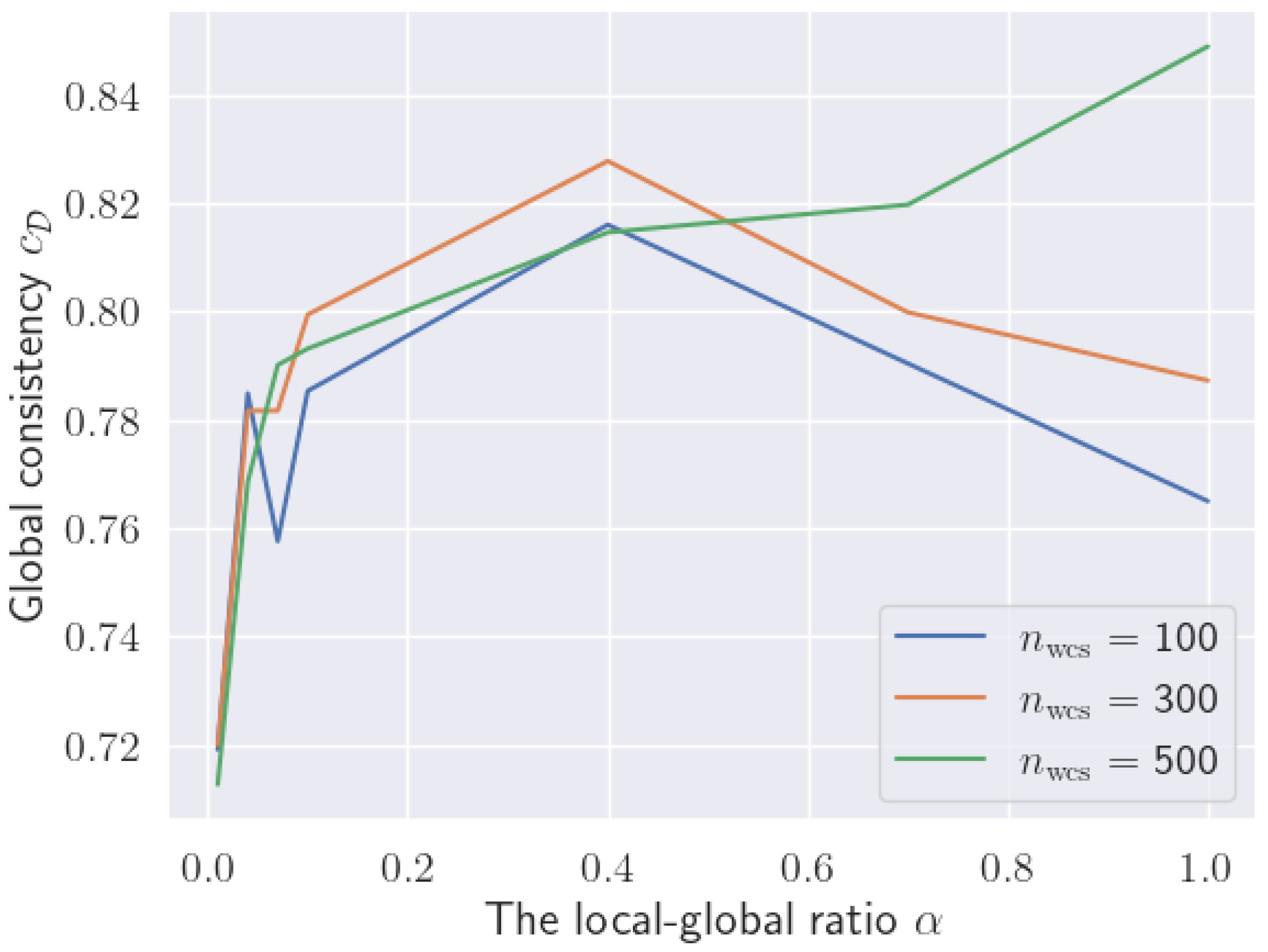
Global consistency level : In contrast to the local consistency level , the global consistency level of MSqC(WCS) is comparable to that of MSGC(B&B) and MSqC(B&B). Moreover, advantages can be observed when is small (e.g., 0.01, 0.04), corresponding to larger distributed systems where each local dataset is significantly smaller than the global dataset.
In addition, similar to the local consistency level
, the global consistency levels
of MSqC(WCS) solutions can also be raised by increasing the WCS sub-problem sizes
, as demonstrated in
Figure 7.
For , the scenario is equivalent to the absence of distributed storage, with models being solved directly using the global dataset.
6. Conclusions
In conclusion, this paper presents an improved summary–explanation (SE) decision support method that aims to promote trust in critical decision-making domains such as credit evaluation. Our method addresses the challenges associated with globally consistent SE by formulating the MSqC problem, which yields SEs achieving substantially higher support in exchange for marginally reduced consistencies. The major contributions of this study are as follows:
- 1.
Methodologically, this paper formulates the MSqC problem for the first time and proposes a novel solution method for MSqC, which not only yield SEs with much greater support, but is also much more scalable in efficiency.
- 2.
From a practical standpoint, this paper offers a valuable tool for decision-makers to generate high-level summaries of datasets and clear explanations of suggested decisions. By generating SE with greater support, this tool can improve the reliability and trustworthiness of DSS.
While the proposed approach demonstrates clear advantages in support maximization and runtime efficiency, the current method assumes static datasets and does not address dynamic or streaming data scenarios, where SEs may need continuous adaptation. In addition, our current experiments assume i.i.d. sampling between local and global datasets. In real-world applications, such as federated credit scoring or temporal shifts in user behavior, non-i.i.d. data distributions can significantly impact the extrapolation quality of explanations. Extending the framework to accommodate these aspects would further enhance its practical applicability.


