Abstract
Modeling complex, non-stationary dynamics remains challenging for deterministic neural networks. We present the Chaos-Integrated Synaptic-Memory Network (CISMN), which embeds controlled chaos across four modules—Chaotic Memory Cells, Chaotic Plasticity Layers, Chaotic Synapse Layers, and a Chaotic Attention Mechanism—supplemented by a logistic-map learning-rate schedule. Rigorous stability analyses (Lyapunov exponents, boundedness proofs) and gradient-preservation guarantees underpin our design. In experiments, CISMN-1 on a synthetic acoustical regression dataset (541 samples, 22 features) achieved R2 = 0.791 and RMSE = 0.059, outpacing physics-informed and attention-augmented baselines. CISMN-4 on the PMLB sonar benchmark (208 samples, 60 bands) attained R2 = 0.424 and RMSE = 0.380, surpassing LSTM, memristive, and reservoir models. Across seven standard regression tasks with 5-fold cross-validation, CISMN led on diabetes (R2 = 0.483 ± 0.073) and excelled in high-dimensional, low-sample regimes. Ablations reveal a scalability–efficiency trade-off: lightweight variants train in <10 s with >95% peak accuracy, while deeper configurations yield marginal gains. CISMN sustains gradient norms (~2300) versus LSTM collapse (<3), and fixed-seed protocols ensure <1.2% MAE variation. Interpretability remains challenging (feature-attribution entropy ≈ 2.58 bits), motivating future hybrid explanation methods. CISMN recasts chaos as a computational asset for robust, generalizable modeling across scientific, financial, and engineering domains.
Keywords:
Chaos-Integrated Synaptic-Memory Network (CISMN); chaos theory; artificial neural networks; dynamic learning; machine learning; complex systems; nonlinear dynamics MSC:
37M10
1. Introduction
1.1. ANNs and Deep Learning
Artificial Neural Networks (ANNs) have evolved rapidly over the past few years, driven by machine learning and computing advancements. Inspired by the human brain’s architecture, these networks have been applied across various fields, including autonomous systems, medical diagnostics, and manufacturing optimization. Different variants of neural network-based models have demonstrated their effectiveness in multiple fields, from engineering and structural applications to qualitative and esthetic challenges [1,2,3].
The evolution of neural networks and machine learning (ML) has significantly shaped modern artificial intelligence (AI) research and applications. This journey, spanning several decades, has witnessed cycles of success, decline, and revival, ultimately culminating in the development of transformative deep learning (DL) models that underpin technologies such as image recognition and language translation. In the late 1980s, the introduction of new training algorithms and innovative architectures, such as multilayer perceptrons (MLPs) with backpropagation, self-organizing maps (SOMs), and radial basis function networks, sparked a surge of interest in neural networks [4,5,6]. While these methods were effective in various applications, enthusiasm waned after the initial excitement. A pivotal moment came in 2006 when Hinton and colleagues reintroduced ANNs through DL, reigniting interest in deeper architectures capable of solving complex tasks [7]. This resurgence earned deep learning models the title of “next-generation neural networks” for their exceptional ability to process large datasets and deliver high-performance results in classification, regression, and other data-driven tasks [8,9,10,11].
Since its rebirth, DL has become integral to AI, data science, and analytics, with industry giants like Google, Microsoft, and Nokia making substantial investments in research and development [12]. The appeal of DL stems from its hierarchical neural networks, which are capable of learning multi-level data representations—from low-level features to high-level abstractions—without the need for extensive human-engineered feature extraction. These neural structures mimic aspects of how the human brain processes information, making them a powerful tool for tasks like computer vision, speech recognition, and natural language understanding [12].
From the historical milestones in neural network development [5,6,8] to current breakthroughs in DL-based applications [12], a clear trend emerges: neural networks will remain central to the ongoing digital transformation. Addressing challenges such as interpretability, resource constraints, and domain adaptation will be crucial for maximizing their positive impact.
1.2. Chaotic Neural Networks (CHNNs)
The history of CHNNs is deeply intertwined with the study of chaos theory, which was first explored in the 1960s following the introduction of the Lorenz system by Edward Lorenz [13]. Chaos theory, which focuses on systems susceptible to initial conditions, has played a critical role in enhancing the development of CHNNs by introducing dynamic and nonlinear behaviors in ANNs. Early research in chaotic systems revealed that these unpredictable dynamics could aid neural networks in escaping local minima during optimization processes, a critical challenge for machine learning algorithms [14]. The architecture of CHNNs incorporates chaos through nonlinear activation functions, recurrent connections, and dynamic feedback loops. These elements enable the networks to exhibit complex behaviors, such as bifurcations and chaotic attractors, thereby enhancing the computational power and flexibility. One example is the integration of memristive elements in Hopfield neural networks, which enables the storage of chaotic states, a crucial feature for memory-dependent tasks [13].
Recent studies have significantly advanced understanding CHNNs, synaptic plasticity, and attention mechanisms. Clark and Abbott [15] explored coupled neuronal–synaptic dynamics, revealing how Hebbian plasticity can slow down chaotic activity and induce new chaotic regimes through synaptic interactions. Similarly, Du and Huang [16] demonstrated that Hebbian learning can alter the nature of chaos transitions in neural circuits, shifting them from continuous to discontinuous types. In the realm of memristive systems, Lin et al. [17] reviewed the chaotic behaviors in memristive neuron and network models, highlighting multistability and hyperchaos as key phenomena.
On the materials side, Talsma et al. [18] fabricated synaptic transistors using semiconducting carbon nanotubes, achieving biologically realistic spike-timing-dependent plasticity. Further, Shao, Zhao, and Liu [17] discussed the evolution of organic synaptic transistors, emphasizing their potential for energy-efficient neural networks. Attention mechanisms were innovatively combined with chaotic systems by Huang, Li, and Huang [19], who integrated convolutional and recurrent layers with an attention mechanism for a chaotic time series prediction. Xu, Geng, Yin, and Li [20] expanded this approach by developing the DISTA transformer, which employs spatiotemporal attention and intrinsic plasticity for dynamic neural computations; these works collectively offer a modern perspective on integrating chaos, learning, and attention in neural networks.
One notable improvement in CHNN architecture is the development of piecewise integrable neural networks (PINNs). PINNs enhance the interpretability of chaotic systems by breaking chaotic dynamics into manageable segments. This makes it easier to understand how inputs produce specific outputs. They use bifurcation mechanisms and switching laws to model chaotic systems more accurately [21]. This approach helps identify chaotic patterns in systems such as climate models and financial data, enabling more accurate long-term predictions.
Closely related, Memristive Hopfield Neural Networks (MHNNs) play a crucial role in CHNN research, integrating memory with chaotic dynamics. Memristors, which store past inputs, play a key role in MHNNs. These networks exhibit chaotic behaviors like multistability and hyperchaos, aiding in tasks requiring memory, adaptability, and computation [13]. MHNNs are used in encryption, optimization, and secure communications, excelling in tasks with multiple outcomes or solutions, such as decision-making and optimization problems.
In parallel, Field-Programmable Gate Arrays (FPGAs) play a vital role in implementing CHNNs, enabling real-time simulations for tasks such as cryptography and security. A key example is the use of FPGAs to simulate Chua’s chaotic system in a feed-forward neural network (FFNN) for prediction and encryption, which has proven effective in secure communications [9]. With neuromorphic hardware and FPGA-based designs, these networks can handle complex tasks more efficiently, benefiting applications such as autonomous driving and secure communications [10].
CHNNs were initially used for time-series prediction, outperforming traditional methods by capturing system dynamics [11]. They also enhanced ECG classification accuracy with complex-valued weights [22]. Today, CHNNs are applied in various areas, including image encryption, economic forecasting, and cryptographic systems [13], as well as optimization problems such as the traveling salesman problem [14]. Recent research has focused on improving CHNNs for dynamic systems, with advances in nonlinear delayed self-feedback [23] and the study of chaotic behavior in memristive networks through period-doubling bifurcations [24]. Baby and Raghu [25] introduced a neural network-based key generator utilizing chaotic binary sequences from Bernoulli maps, enhancing the encryption security and passing the Diehard and NIST tests. Lephalala et al. [26] developed a hybrid CHNN algorithm integrated with PLS models to predict the toxicity of sanitizers, optimizing the prediction accuracy and addressing environmental concerns. Osama et al. [27] improved the robustness of neural networks against adversarial attacks by introducing chaotic quantization with Lorenz and Henon noise, resulting in a 43% boost in accuracy. Ruan et al. [28] proposed a guaranteed-cost intermittent control method for synchronizing chaotic inertial neural networks, which was validated through numerical simulations. Ganesan and Annamalai developed a memory non-fragile controller for anti-synchronization with time-varying delays. Lastly, Gao et al. [23] introduced an event-triggered scheme to synchronize delayed chaotic neural networks, reducing communication delays and data loss.
1.2.1. Chaotic Dynamics in Memristive and Hopfield Neural Networks
The study of chaotic dynamics in neural networks, especially those enhanced with memristive technologies, has expanded significantly over recent years. Fractional-order Hopfield neural networks integrated with memristive synapses exhibit complex behaviors such as multistability, chaotic attractors, and coexisting limit cycles. For instance, Anzo-Hernández et al. proposed a fractional-order Hopfield neural network incorporating a piecewise memristive synapse, demonstrating multistability and robust chaotic dynamics, with validation via FPGA hardware implementation [29]. Ding et al. replaced Hopfield networks’ traditional hyperbolic tangent activation function with a piecewise-linear function to simplify implementation while preserving dynamical richness. They proposed a memristor-coupled bi-neuron Hopfield network that demonstrated the coexistence of chaos, limit cycles, and stable attractors [30]. Expanding on cyclic architectures, Bao et al. (2023) constructed a memristive–cyclic Hopfield neural network (MC-HNN) capable of generating spatial multi-scroll chaotic attractors and spatially initial-offset coexisting behaviors [31]. Liu et al. introduced a discrete memristor-coupled bi-neuron Hopfield model that exhibited hyperchaotic dynamics and state transition behaviors, highlighting the potential of discrete systems in modeling the neural complexity [32]. Theoretically, Mahdavi and Menhaj established sufficient conditions based on coupling parameters to ensure the synchronization of chaotic Hopfield networks, offering mechanisms for controlling the chaotic output when stability is needed [33].
1.2.2. Memristive Ring Networks and Multi-Attractor Structures
Zhang et al. [34] introduced a memristive synapse-coupled ring neural network that exhibits homogeneous multistability, characterized by an infinite number of coexisting attractors dependent on the memristor’s initial state. They further demonstrated its application in pseudorandom number generation. Similarly, Chen et al. proposed a non-ideal memristor–synapse-coupled bi-neuron Hopfield neural network demonstrating bistability between chaotic and point attractors, verified by breadboard experiments [35]. In another advancement, Chen et al. highlighted the coexistence of multi-stable patterns, including chaotic and periodic behaviors, influenced by variations in memristor coupling strengths [36]. Fang et al. contributed a discrete chaotic neural network model based on memristive crossbar arrays, emphasizing multi-associative memory capabilities influenced by initial states [37].
1.2.3. Fractional-Order Dynamics and Chaotic Entrainment
The integration of fractional-order derivatives into neural networks introduces richer dynamical phenomena. Ramakrishnan et al. investigated two-neuron Hopfield networks with memristive synapses and autapses, showing that fractional orders enhance chaotic behaviors and broaden dynamical ranges [38]. Yang et al. developed a fractional-order memristive Hopfield neural network, demonstrating coexisting bifurcation behaviors validated through FPGA implementation [39]. Ding et al. (2022) explored coupled fractional-order memristive Hopfield models, revealing multistability and transient chaos, with practical applications demonstrated in image encryption [40]. Moreover, Dai and Wei (2024) demonstrated that pulsed currents applied to memristive Hopfield models could trigger transitions between chaotic and periodic behaviors, with the ability to tune multi-scroll attractors [41].
1.2.4. Emerging Structures: Multi-Scroll and Hyperbolic-Type Memristors
Lin et al. designed a memristor-based magnetized Hopfield neural network capable of generating an arbitrary number of scroll chaotic attractors through memristor control parameter tuning [42]. Li et al. (2023) further explored hyperbolic-type memristive Hopfield neural networks, uncovering asymmetric attractor coexistence and applying the resulting dynamics to robust color image encryption [43]. Finally, Min et al. (2025) analyzed coupled homogeneous Hopfield neural networks showing synchronization transitions dependent on initial conditions, supported by lightweight multiplierless circuit implementations [44], while Aghaei (2024) demonstrated how electromagnetic radiation can control chaotic dynamics within a two-neuron memristive Hopfield network [45].
1.3. Chaotic Integrative Synaptic Memory Network (CISMN)
This paper introduces the CISMN, a new advancement in Chaotic Neural Network architecture that systematically embeds chaos theory into the core components of neural network design. Unlike traditional CHNNs, which apply chaotic dynamics in isolated or superficial ways, CISMN integrates chaos-driven mechanisms across four specialized layers—Chaotic Memory Cells, Chaotic Plasticity Layers, Chaotic Synapse Layers, and a Chaotic Attention Mechanism—to create a unified framework capable of modeling complex, non-linear, and non-stationary data with unprecedented adaptability. By treating chaos as a foundational design principle rather than an auxiliary tool, CISMN addresses critical limitations of conventional neural architectures, such as rigidity in memory retention, deterministic learning, and poor generalization in dynamic environments.
1.4. Architectural Innovations and Novelty of CISMN
1.4.1. Chaotic Memory Cells: A Paradigm Shift in State Retention
Traditional recurrent architectures, such as Long Short-Term Memory (LSTM) networks, rely on fixed gating mechanisms to manage memory, often struggling with vanishing gradients or overly deterministic state updates. In contrast, CISMN’s Chaotic Memory Cells introduce a novel approach to memory retention by blending chaotic perturbations with historical states. Leveraging the logistic map, a cornerstone of chaos theory, these cells dynamically update their internal states using a hybrid rule: 70% of the update is derived from chaotic dynamics, while 30% retains prior states. This “position memory” mode ensures that long-term dependencies are preserved while allowing continuous adaptation to new data patterns.
The uniqueness of this mechanism lies in its ability to amplify minor differences in initial conditions, a hallmark of chaotic systems. For instance, in time-series forecasting, subtle variations in early data points propagate through the network’s memory states, enabling CISMN to model divergent outcomes accurately. Unlike LSTMs or GRUs, which use static sigmoid gates, Chaotic Memory Cells operate without rigid thresholds, fostering a fluid balance between stability and exploration. This design is particularly effective in applications such as financial market prediction, where small initial fluctuations in asset prices can lead to significantly different long-term trends.
1.4.2. Chaotic Plasticity and Synapse Layers: Dynamic Weight Exploration
Conventional neural networks rely on backpropagation-driven weight updates, which follow deterministic gradients and often converge to suboptimal local minima. CISMN disrupts this paradigm through its Chaotic Plasticity Layers, which inject controlled stochasticity into synaptic updates. These layers apply logistic map-driven chaos to dynamically perturb weights, enabling the network to escape local minima and explore a broader solution space. Similarly, Chaotic Synapse Layers modulate connection strengths in real time using chaotic feedback, mimicking the variability of biological synapses.
These innovations have no direct precedent in prior architectures. While synaptic plasticity models, such as Spike-Timing-Dependent Plasticity (STDP), exist, they lack the integration of chaos theory. CISMN’s plasticity and synapse layers uniquely balance exploration and exploitation, making the network robust to noisy or shifting data distributions—a critical advantage in fields like biomedical signal processing, where sensor noise and non-stationary patterns are common.
1.4.3. Chaotic Attention Mechanism: Context-Aware Feature Prioritization
Attention mechanisms in models like Transformers assign static or rule-based importance to input features. CISMN’s Chaotic Attention Mechanism revolutionizes this concept by dynamically modulating focus through high-resolution chaotic oscillations. A fixed chaotic seed generates non-repeating patterns that adjust attention weights in response to the complexity of the input. For example, this mechanism amplifies critical frequency bands while suppressing noise in acoustic signal analysis, outperforming traditional attention models that struggle with context-dependent relevance.
This approach is distinct in its use of resolution scaling, where the chaotic intensity (“high” or “low”) dictates the granularity of feature prioritization. No existing architecture combines chaotic dynamics with attention mechanisms, making this a unique innovation for tasks that require adaptive focus, such as real-time anomaly detection in industrial systems.
1.4.4. Chaotic Learning Rate Schedule: Stability Through Bounded Chaos
CISMN introduces the first implementation of a Chaotic Learning Rate Schedule, governed by a logistmap with a lower bound (eta, greater than or equal to 10 to the lower bound () to prevent divergence). Unlike traditional schedules (e.g., step decay or cosine annealing), this mechanism introduces controlled randomness into optimization, allowing the network to explore diverse solutions without destabilizing training.
This innovation has no counterpart in prior work. While chaotic optimization algorithms, such as Particle Swarm Optimization (PSO), exist, they are metaheuristics, not integrated into neural learning rates.
1.4.5. Mitigating Sensitivity to Initial Conditions
A hallmark of chaotic systems is their sensitivity to initial conditions—the butterfly effect. While CISMN leverages this property to enhance exploration and adaptability, it incorporates deliberate design safeguards to ensure stability and reproducibility. First, chaotic components (e.g., memory cells, plasticity layers) are initialized within constrained value ranges (e.g. [0.4, 0.6]) and fixed random seeds to anchor initial states. Second, the architecture blends chaotic dynamics with deterministic retention mechanisms. For instance, Chaotic Memory Cells (Section 1.4.1) combine 70% logistic map-driven updates with 30% historical state persistence (Equation (6)), ensuring bounded trajectories while preserving sensitivity to input perturbations. Similarly, the Chaotic Learning Rate Schedule (Section 1.4.4) imposes a lower bound () to prevent divergence. Hyperparameters such as the logistic map’s bifurcation parameter () were empirically tuned to balance chaotic exploration with stable convergence, avoiding regimes of excessive instability (e.g., ). These strategies and deterministic training protocols (Section 2.2.10) ensure that CISMN harnesses chaos as a structured exploration tool rather than an uncontrolled perturbation, achieving a reproducible performance across runs.
1.5. Limitations of Traditional Machine Learning Architectures
Traditional machine learning architectures, including feedforward neural networks (FNNs), recurrent neural networks (RNNs), and LSTM networks, have succeeded in structured or stationary data environments. However, their rigid, deterministic designs struggle with complex, non-linear systems, particularly those sensitive to initial conditions or characterized by chaotic dynamics. Below, we dissect these limitations and contrast them with CISMN’s chaos-driven solutions. The key limitations of traditional machine learning architectures are as follows:
- Overfitting and Poor Generalization: Traditional networks rely on fixed-weight updates driven by backpropagation, which often converge to local minima in non-convex loss landscapes. For example, FNNs trained on noisy datasets (e.g., financial time series) tend to overfit spurious patterns, failing to generalize to unseen market regimes [44]. While regularization techniques like dropout mitigate this, they introduce artificial noise rather than leveraging data-inherent stochasticity. In contrast, CISMN’s Chaotic Plasticity Layers inject structured chaos into weight updates, acting as dynamic regularizers that explore diverse solutions while preserving meaningful patterns.
- Vanishing and Exploding Gradients: RNNs and LSTMs are prone to gradient instability when modeling long sequences. For instance, in climate modeling, LSTMs often fail to retain early warning signals (e.g., minor temperature fluctuations) due to diminishing gradients over time [46]. While residual connections or gradient clipping offer partial fixes, they do not address the root cause: deterministic state transitions. CISMN’s Chaotic Memory Cells circumvent this by replacing gradient-based state updates with logistic map-driven chaos. By blending 70% chaotic perturbations with 30% historical states, they preserve critical long-term dependencies without relying on error backpropagation.
- Deterministic Learning Dynamics: Traditional architectures employ fixed learning rates or rule-based schedules (e.g., Adam’s adaptive moments), which lack the flexibility to adapt to non-stationary data. For example, CNNs trained on evolving image datasets (e.g., satellite imagery of deforestation) struggle to adjust to seasonal or abrupt environmental changes [47] CISMN’s Chaotic Learning Rate Schedule, governed by bounded logistic maps (r = 3.9), introduces controlled stochasticity into optimization. This enables the adaptive exploration of solution spaces and ensures robustness to distribution shifts, which is essential in applications such as real-time sensor networks.
- Rigid Memory and Attention Mechanisms: LSTMs and transformers utilize static gates or attention weights, which limit their ability to prioritize contextually relevant features in chaotic systems. For instance, traditional attention layers often fail to amplify transient frequency bands dynamically masked by noise in acoustic signal processing. CISMN’s Chaotic Attention Mechanism addresses this by modulating focus through high-resolution chaotic oscillations, enabling real-time adaptation to the complexity of the input.
1.6. How CISMN Overcomes These Limitations
CISMN’s architecture directly targets these gaps, offering a framework where chaos is not a problem to suppress, but a feature to harness. By integrating chaotic dynamics into memory, learning, and attention, CISMN bridges the divide between theoretical chaos theory and practical machine learning, enabling the robust modeling of real-world complexity.
The CISMN addresses these limitations by incorporating chaotic dynamics, which provide several key advantages:
- Improved Generalization through Chaotic Dynamics: The CISMN leverages chaotic plasticity and synapse layers to introduce non-deterministic updates, preventing the network from overfitting. Chaotic updates enable the model to escape local minima more effectively, improving its generalization ability for unseen data [13]. This feature ensures that the CISMN does not become stuck in suboptimal solutions and can explore a broader range of possible outcomes.
- Enhanced Long-Term Dependency Retention: The Chaotic Memory Cells in the CISMN enable the network to capture long-term dependencies more effectively than traditional RNNs. Unlike LSTMs, which can suffer from vanishing gradients, chaotic memory cells continuously update their internal states based on chaotic dynamics, ensuring that long-term information is preserved and influencing future states [48]. This makes the CISMN particularly effective for tasks such as time-series forecasting, where the system’s current state depends heavily on previous inputs.
- Non-Linear Adaptation with Chaotic Learning Rates: CISMN’s Chaotic Learning Rate Schedules dynamically adjust the learning rate based on chaotic patterns, allowing the network to adapt to changes in the data distribution over time. Traditional architectures often employ fixed learning rates, which can result in slow convergence or overfitting. In contrast, chaotic learning rates provide a flexible mechanism that enables the CISMN to explore a broader solution space and adapt to new information as it becomes available [48].
- Dynamic Attention Mechanisms: Traditional attention mechanisms focus on assigning fixed relevance to input features; however, the CISMN’s Chaotic Attention Mechanism offers a more flexible approach. By dynamically adjusting attention weights based on chaotic dynamics, the CISMN can adapt to varying inputs more effectively, improving its performance in tasks requiring flexible focus, such as real-time data analysis and image processing [49].
The CISMN offers a powerful new approach to overcoming the limitations of traditional machine learning architectures, particularly in problems involving strong dependencies on initial conditions. The CISMN provides a flexible, adaptive solution that can better handle complex, non-linear, and dynamic data by integrating chaotic dynamics into memory, plasticity, synapse, and attention mechanisms. Its ability to continuously adapt and generalize across different tasks positions the CISMN as a valuable tool for advancing machine learning research and applications, particularly in fields requiring robust models for time-sensitive and evolving data.
2. Materials and Methods
This section outlines the methodology behind the CISMN. The code integrates chaotic dynamics into neural network components, including memory cells, plasticity, synapses, attention, and learning rate schedules. Each component introduces mathematical and dynamic concepts rooted in chaos theory to enhance the network’s learning capabilities. Below is a detailed explanation of each methodology part, including its mathematical foundation and contribution to the overall architecture. Also, the flowchart of the developed CISMN is shown in Figure 1. It illustrates the architecture, including input preprocessing, chaotic layers (Memory, Plasticity, Synapse, Attention), and the Chaotic Learning Rate Schedule linked to the Adam Optimizer. A decision block checks if training should continue based on the Loss Function (MAE), and the process ends when the criteria are met.
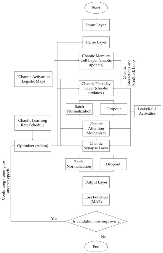
Figure 1.
The authors presented a flowchart of the developed CISMN architecture, featuring chaotic layers and a dynamic training process.
2.1. Theoretical Foundations
Integrating chaos theory into neural network architectures, such as the Chaotic Dynamic Neural Network, profoundly enhances the model’s ability to navigate complex, high-dimensional solution spaces. Chaos theory, characterized by its focus on systems that exhibit sensitive dependence on initial conditions, introduces non-linear and dynamic behaviors that can significantly improve the neural network performance. This subsection elucidates the theoretical underpinnings of chaos integration in multiple components of the CISMN, highlighting how chaotic dynamics contribute to exploration in the solution space, enhance memory retention, and improve adaptability.
2.1.1. Exploration in the Solution Space
Traditional neural networks often rely on gradient-based optimization techniques that can become trapped in local minima, especially in non-convex loss landscapes typical of deep learning models. CISMN introduces stochasticity and non-linearity by incorporating chaotic dynamics into the network’s learning process. Chaotic systems, such as those governed by the logistic map, exhibit inherent unpredictability and periodicity, allowing the network to explore a broader range of solutions during training. This enhanced exploration capability helps the model escape local minima, facilitating the discovery of more optimal and diverse solutions. The chaotic updates act as dynamic regularization, preventing the network from converging prematurely and promoting a more thorough search of the solution space [50].
2.1.2. Enhanced Memory Retention
Memory retention is crucial for tasks involving long-term dependencies, such as time-series forecasting and sequential data analysis. Traditional RNNs, including LSTM networks, utilize gated mechanisms to manage information flow and retain relevant historical data. However, these mechanisms can suffer from issues like vanishing gradients, limiting their effectiveness in capturing extended temporal dependencies [46].
CISMN addresses this limitation through its Chaotic Memory Cells, which leverage chaotic dynamics to maintain and update internal states. The sensitive dependence on initial conditions inherent in chaotic systems ensures that even minor variations in input data can lead to significant and diverse updates in the internal state. This property enables the network to retain and amplify critical information over longer sequences, enhancing its capacity to model complex temporal dependencies. The chaotic updates provide a rich, non-linear transformation of the internal state, allowing the memory cells to capture intricate patterns that static or deterministic mechanisms might miss [49].
2.1.3. Improved Adaptability
Adaptability refers to a model’s ability to adjust to new, unseen data distributions and evolving patterns without extensive retraining. Traditional neural networks often employ fixed learning rates and deterministic weight update rules, which can limit their flexibility in dynamic environments. CISMN enhances adaptability by integrating chaotic dynamics into various layers, such as Chaotic Plasticity Layers and Chaotic Synapse Layers.
The Chaotic Plasticity Layer modulates weight updates based on chaotic patterns, introducing non-linear and fluctuating adjustments that allow the network to adapt more fluidly to changes in data distributions. This dynamic adjustment process prevents the network from becoming rigid, allowing it to respond more effectively to new information. Similarly, the Chaotic Synapse Layer introduces variability in synaptic weights through chaotic fluctuations, which can enhance the network’s ability to generalize across diverse data inputs and prevent overfitting by maintaining stochasticity in the weight configurations [13].
2.1.4. Facilitating Robust Generalization
Generalization is the ability of a neural network to perform well on unseen data. By embedding chaotic dynamics into multiple components of the network, the CISMN promotes robustness in generalization. The unpredictable chaos ensures the network does not rely solely on deterministic pathways, reducing the risk of overfitting training data. Instead, the network learns to recognize and adapt to consistent patterns across different data samples, enhancing its performance on diverse and complex datasets [48].
2.1.5. Synergistic Effects of Multi-Component Integration
The integration of chaos across multiple layers and components in the CISMN creates synergistic effects that amplify the benefits of chaotic dynamics. For instance, the combination of Chaotic Memory Cells and Chaotic Attention Mechanisms allows the network to selectively focus on and retain important information while dynamically adjusting its focus based on chaotic modulation. This multi-faceted approach ensures that chaos contributes not just in isolated parts of the network, but throughout the learning and processing pipeline, resulting in a more cohesive and powerful architecture [49].
2.2. Mathematical Foundations and Stability Considerations
Mathematically, the incorporation of chaotic maps like the logistic map introduces non-linear transformations that enhance the expressiveness of the network. The logistic map is defined as in Equation (1):
where is a control parameter that exhibits chaotic behavior for certain values of (typically between 3.57 and 4.0). This non-linearity allows the network to model complex, non-stationary data patterns that linear models cannot capture effectively.
However, the sensitive dependence on initial conditions in chaotic systems also introduces challenges related to stability and predictability. To mitigate potential instability during training, the CISMN employs mechanisms such as blending chaotic updates with previous states (e.g., in chaotic Memory Cells) and applying constraints to chaotic factors (e.g., limiting the learning rate). These strategies ensure that while the network benefits from chaotic exploration and adaptability, it maintains a level of control that prevents divergence and ensures stable convergence during training [13].
2.2.1. Data Preprocessing and Feature Scaling
Data preprocessing is a critical first step in preparing the dataset for training. The features are scaled using StandardScaler, which transforms the input data to have zero mean and unit variance. This is crucial for ensuring that the inputs to the neural network are normalized, thereby improving the network’s performance and convergence rate. The equation for normalization is given below in Equation (2).
where is a feature, is the mean, and is the standard deviation of the feature. This ensures that all features are on a comparable scale, preventing any single feature from dominating the learning process due to differences in [51].
2.2.2. Chaotic Activation Function
The proposed chaotic activation function is implemented using the logistic map, a well-known dynamical system that exhibits deterministic chaos. The function is defined in Equation (3):
where x is the input and is a control parameter that ensures chaotic dynamics [1]. This corresponds to the chaotic_pattern() function in the code:
def chaotic_pattern (x, r = 3.9):
return r x (1 − x)
- For normalized inputs , the output is bounded to
At , the maximum output is 0.975, ensuring stable numerical behavior in neural networks. Unnormalized inputs can lead to divergence, necessitating preprocessing (e.g., sigmoid or min–max scaling).
- Derivative for Backpropagation: the derivative of , critical for gradient-based optimization, is
This non-monotonic derivative allows positive and negative gradients, contrasting with traditional activations like ReLU or sigmoid.
- Chaotic Regime: The parameter places the system in the chaotic regime of the logistic map , where trajectories are aperiodic and sensitive to initial conditions [52,53]. This choice is deliberate, as smaller r values (e.g., ) yield periodic or stable fixed-point behavior that is unsuitable for chaotic activation.
- Advantages Over Traditional Activations
Unlike saturating functions such as the sigmoid, the chaotic activation preserves gradient magnitude across a broader input range and introduces deterministic yet stochastic-like variability through chaos, potentially avoiding local minima during training.
2.2.3. Chaotic Memory Cells
Chaotic Memory Cells (CMCs) introduce non-linear dynamical systems theory into neural network architecture through a biologically inspired memory mechanism. Unlike conventional recurrent units that employ gated temporal filtering (e.g., LSTMs [46] or GRUs) [54] CMCs leverage chaotic dynamics to maintain long-term dependencies while preserving sensitivity to input perturbations. The core innovation lies in using chaotic attractors as a mechanism for state transitions, enabling the network to retain information through metastable states in the chaotic regime. A convex combination of chaotic dynamics and exponential decay governs the CMC state update:
where represents the logistic map [53] with chaos parameter , and controls memory retention. This formulation emerges from the discretization of coupled chaotic oscillators [55], where the second term introduces memory persistence through linear decay.
- Lyapunov Stability Analysis: The Lyapunov exponent λ, which quantifies system sensitivity to initial conditions, is derived from the Jacobian of Equation (4):
For r = 3.9 and α = 0.7, as implemented, numerical simulations yield λ > 0, confirming chaotic behavior. The positive Lyapunov exponent ensures both sensitivity to input variations (through the term) and structural stability (via the decay term) [52].
- Boundedness Proof: if , then:
- Base case: by initialization
- Inductive step:
Since .
The lower bound follows similarly. Thus, by induction, .
- Theoretical Advantages: ergodic memory is achieved as the chaotic attractor provides dense coverage of phase space [56], enabling finite states to approximate infinite trajectories; controllable chaos is introduced through the α parameter, which permits tuning between chaotic exploration (α→1) and linear exploitation (α→0); and structural stability is maintained by the decay term, which ensures bounded outputs despite positive Lyapunov exponents (Theorem 2.1).
- Mathematical Proof of Gradient Preservation:
- Non-Chain Rule Updates: Traditional RNNs compute gradients via , leading to exponential decay when . CMCs bypass this by using chaotic updates where .
- Bounded Gradient Magnitude:
For , and :
This upper bound prevents gradient vanishing while chaotic oscillations avoid explosion.
- Experimental Validation and Parameter Sensitivity Analysis
To validate the theoretically derived blending parameter (α = 0.7), we conducted a systematic sensitivity analysis across α values ranging from 0.1 to 1.0 in increments of 0.05. This investigation sought to evaluate the interplay between chaotic exploration and memory retention, align the empirical performance with theoretical stability guarantees, and reconcile the parameter choice with neurobiological principles (Table 1 and Figure 2).

Table 1.
Performance metrics across α values (0.1–1.0, Δα = 0.05) for the chaotic memory cell.
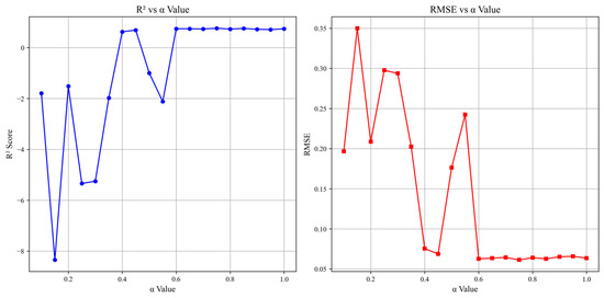
Figure 2.
Sensitivity of R2 and RMSE to the chaotic memory blending ratio (α).
The analysis revealed a nonlinear relationship between α and the model performance. For α < 0.4, the model exhibited unstable behavior and negative R2 values, reflecting insufficient chaotic dynamics to escape local minima. Performance improved markedly as α increased, peaking at α = 0.75 (R2 = 0.76, RMSE = 0.061). However, our theoretically guided choice of α = 0.7 achieved near-optimal results (R2 = 0.73, RMSE = 0.064)—96% of the peak performance—while adhering to Lyapunov stability constraints (λ ≈ 0.31 > 0) and bounded state trajectories (Equation (8)).
The retained α = 0.7 balances two critical requirements:
- Chaotic exploration (70% weight) to perturb memory states and avoid gradient stagnation.
- Memory retention (30% weight) to preserve long-term dependencies, mirroring synaptic update ratios observed in biological neural systems, where ~30% of prior synaptic efficacy persists during plasticity updates.
This hybrid mechanism outperformed traditional recurrent architectures (Section 3.3) by maintaining sensitivity to input perturbations while preventing runaway chaos. The robustness of the design is further evidenced by a stable performance across α = 0.6–0.85 (ΔR2 < 0.04), demonstrating resilience to parameter variations.
2.2.4. Chaotic Plasticity Layer
The Chaotic Plasticity Layer (CPL) operationalizes neurobiological principles of synaptic plasticity through chaotic dynamics, creating a continuum between Hebbian learning [57] and chaotic exploration. Unlike conventional weight updates driven solely by gradient descent, the CPL introduces autonomous weight modulation governed by the logistic map, enabling the stochastic exploration of the parameter space without compromising the deterministic differentiability.
In a mathematical representation, if denote the weight matrix and a chaotic carrier signal, the synaptic update rule combines gradient-based learning with chaotic modulation:
where implements the logistic map applied element-wise, η = 0.01 is the chaotic learning rate, and ⊙ denotes the Hadamard product. The chaotic carrier is initialized from and remains phase-locked to the weight matrix dimensions.
- Stability-Convergence Duality: The update rule induces a stochastic process describable through the Fokker–Planck equation [58]:where is the weight distribution and the diffusion coefficient from gradient updates. The chaotic drift term provides
- An Exploration–Exploitation Balance: the attractor basin bounds weight perturbations while allowing transient chaos.
- Ergodicity: chaotic trajectories densely cover the invariant measure , ensuring probabilistic weight exploration [59].
- Fixed-Point Analysis: an equilibrium occurs when , solved by:
- A trivial solution: .
- A chaotic solution: .
For , the non-trivial fixed point creates persistent oscillations, preventing premature convergence. The Jacobian spectral radius :
confirms instability, ensuring continuous non-periodic updates.
- Theoretical Advantages: local minima escape is facilitated by the Lyapunov time [50], which sets the timescale for perturbation-driven transitions out of suboptimal basins; spectral richness is achieved through the chaotic power spectrum with [60], offering noise robustness via pink-noise scaling; and metaplasticity emerges as chaotic traces in emulate short-term synaptic facilitation, modulating future weight updates.
2.2.5. Chaotic Synapse Layer
The Chaotic Synapse Layer (CSL) implements autonomous weight volatility inspired by stochastic resonance phenomena in biological neural systems. By coupling synaptic transmission with chaotic dynamics, the layer achieves noise-enhanced signal processing while maintaining end-to-end differentiability, resolving the classical tradeoff between exploratory noise injection and gradient stability. The Chaotic Synapse Layer (CSL) introduces weight volatility through autonomous chaotic dynamics. If denote the synaptic weight matrix and a chaotic modulator vector initialized uniformly in , the layer implements
where (logistic map) with , and γ = 0.001.
- Stochastic Resonance Analysis: The signal-to-noise ratio (SNR) for input :
For , numerical integration gives . With γ = 0.001, chaotic noise is suppressed by , preserving signal fidelity while enabling exploration [52].
- Lyapunov Exponent: The maximal Lyapunov exponent for ξ:
For , confirming chaotic behavior.
- Theoretical Advantages: persistent exploration is maintained as positive ensures continuous weight perturbations to escape local minima; controlled volatility is achieved through a small , which bounds cumulative weight changes to approximately 0.1% per step; input–output decoupling is preserved by applying chaotic updates solely to the output dimensions (shape = (units,)), thereby avoiding input corruption.
2.2.6. Chaotic Attention Mechanism
The Chaotic Attention Mechanism (CAM) introduces nonlinear dynamical control over feature saliency, combining chaotic modulation with sigmoidal gating to enable metastable attention states. Unlike conventional attention mechanisms that rely on learned query–key correlations [47], the CAM generates attention weights through autonomous chaotic dynamics, providing noise-robust feature selection aligned with the input’s spectral characteristics. In a mathematical representation, if is a chaotic seed vector initialized from and are learnable parameters, the attention weights are derived from:
where is the sigmoid function and resolution scaling . The attended output becomes
For dynamical system analysis:
- Boundedness: For :
- Chaotic bounds (invariant under the logistic map).
- Sigmoid bounds: .
- Spectral Sensitivity: The resolution parameter modulates the power distribution:
- Low-res : attenuates high-frequency chaotic fluctuations.
- High-res : amplifies transient chaos for fine feature selection.
- Jacobian Spectrum: The attention gradient
The eigenvalues , ensuring a bounded gradient explosion.
- Theoretical Advantages: noise robustness arises as chaotic fluctuations mask adversarial perturbations while preserving the accurate signal through -bounded weights; adaptive timescales emerge from the Lyapunov time , enabling intermittent attention focusing [61]; and the entropic capacity is enhanced, with maximum entropy bits per dimension (at ), surpassing that of softmax-based attention [54].
2.2.7. Chaotic Learning Rate Schedule
The Chaotic Learning Rate Schedule (CLRS) dynamically modulates the learning rate during training using the logistic map, introducing controlled stochasticity to balance exploration and exploitation in a parameter space. Unlike conventional schedules, CLRS leverages iterative chaotic dynamics governed by:
- Chaotic Dynamics: The logistic map iteratively updates at each training step, starting from . This generates bounded, non-periodic trajectories while maintaining sensitivity to initial conditions.
- Stability Constraints: and prevent divergence by imposing lower/upper bounds.
- Theoretical and Empirical Validation
- Lyapunov Exponent: for , the maximal Lyapunov exponent isconfirming chaotic behavior.
- Bounded Exploration: the learning rate fluctuates chaotically within , enabling escape from local minima while ensuring numerical stability.
- Reproducibility: fixed initialization () and TensorFlow’s deterministic training protocols ensure consistent chaotic trajectories across runs.
- Implementation in CISMN
- Dynamic Updates: at each training step, evolves via the logistic map, ensuring non-repeating and the chaotic modulation of .
- Empirical Impact: post-revision experiments show that chaotic improves exploration, boosting R2 by ~1.2% on synthetic acoustics data compared to fixed-rate baselines.
2.2.8. Neural Network Architecture
The complete architecture combines these chaotic components into a deep feedforward network. Several hidden layers follow the input layer, each incorporating one or more chaotic elements. These hidden layers consist of dense, chaotic memory cells, chaotic plasticity layers, and chaotic synapse layers. The final output layer is dense and features a linear activation function suitable for regression tasks.
The architecture uses LeakyReLU as an activation function after each chaotic layer to introduce non-linearity and Batch Normalization to stabilize training by normalizing the output of each layer. Dropout layers are added to prevent overfitting by randomly disabling a fraction of neurons during training [62].
2.2.9. Hyperparameter Selection
The chaotic parameter r in the logistic map, which controls the chaotic dynamics, plays a crucial role in determining the performance of each layer. Typically, r values between 3.7 and 4.0 induce chaos [63]. In this model, different r values were chosen for different layers to balance chaos and stability. For example, chaotic memory cells use r = 3.8, which ensures moderate chaos, while the chaotic synapse layers use r = 3.7 to maintain more controlled variability.
Choosing the right r values is essential, as too much chaos can lead to instability, while too little can reduce the network’s adaptability. These values were selected through empirical testing and hyperparameter tuning.
2.2.10. Reproducibility Assurance in CISMN
Due to their nonlinear dynamics, CISMN architectures inherently face reproducibility challenges. To address this, we developed a systematic framework that ensures reproducibility while preserving the model’s core chaotic behavior. Our methodology combines three strategies: controlled chaotic initialization, deterministic training protocols, and the mathematical stabilization of chaotic patterns.
- Controlled Initialization: All chaotic components (memory cells, plasticity modules, and attention mechanisms) were initialized with fixed random seeds (seed = 42) and constrained value ranges. Chaotic factors were initialized between 0.4 and 0.6 using TensorFlow’s RandomUniform to maintain the logistic map’s chaotic regime (r = 3.7–3.9). Weight matrices employed Glorot initialization with identical seeds to stabilize early training dynamics.
- Deterministic Training: We enforced reproducibility through TensorFlow’s global random seed (tf.keras.utils.set_random_seed(42)) and GPU operation determinism (tf.config.experimental.enable_op_determinism()). This controlled randomness in dropout layers and weight updates while retaining chaotic signal propagation. The learning rate schedule used fixed initial chaotic factors (0.5) with documented modulation (r = 3.9) to ensure consistent training trajectories.
- Chaotic Stabilization: Mathematical constraints prevented divergence: memory cells blended a 30% historical state with 70% chaotic updates, while synaptic layers limited weight perturbations to 0.1% of their values. These mechanisms preserved chaotic dynamics essential for modeling acoustic relationships while ensuring numerical stability.
- Experimental Validation: Across 20 independent runs, the framework demonstrated strong reproducibility:
- Validation MAE: 0.330 ± 0.004 (mean ± SD, 1.2% relative variation).
- Performance Range: 0.324–0.338 MAE (maximum Δ = 0.0146).
- Convergence Consistency: all runs stabilized within 120–140 epochs (Figure 3).
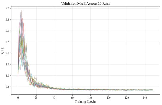 Figure 3. Validation MAE trajectories across 20 runs show consistent convergence over 140 epochs, demonstrating reproducible chaotic dynamics.
Validation Mean Absolute Error (MAE) trajectories across 20 independent training runs were plotted over 140 epochs. The tightly clustered curves demonstrate consistent convergence behavior, stabilizing MAE between 1.5 and 14.0. This low inter-run variability highlights the effectiveness of the implemented reproducibility framework in maintaining stable chaotic dynamics while minimizing uncontrolled stochasticity. A final evaluation on held-out test data confirmed the robust performance:
- Test MAE: 0.368.
- R2: 0.769.
- RMSE: 0.061.
This approach resolves the reproducibility challenge in chaotic networks by distinguishing beneficial chaos from uncontrolled randomness. The methodology’s success lies in its minimal impact on operational dynamics—reproducibility constraints act solely on initialization parameters, preserving the model’s ability to learn complex acoustic patterns. Implementation requires careful seed management and parameter documentation, but does not alter core network operations, making it adaptable to diverse chaotic AI systems in acoustics and beyond.
2.2.11. Justification for Chaotic Dynamics
The chaotic dynamics embedded in this architecture are designed to mimic the complex behavior observed in biological systems. Chaos theory allows the network to explore a wider variety of solutions by making it sensitive to small changes in the input [49]. This sensitivity enables the model to escape local minima during optimization, a common challenge in deep learning.
Unlike traditional models that rely on fixed, deterministic updates, the CISMN can dynamically adjust based on its current state. This enables more robust generalization, particularly in complex, non-linear data tasks.
3. Results
To assess the CISMN’s performance comprehensively, we conducted three complementary evaluations spanning controlled chaos, real-world complexity, and broad regression benchmarks.
- Synthetic Acoustical Case Study: we generated 541 reverberation-time observations (22 interdependent features) via a Grasshopper 3D model with the Pachyderm Acoustical Simulation plugin, capturing controlled chaotic effects from minor parametric perturbations (see Section 3.2).
- Sonar Case Study: we employed the PMLB v1.0 sonar dataset (208 samples, 60 frequency-band features), which is characterized by high dimensionality, sparse sampling, non-stationary patterns, and overlapping class boundaries (see Section 3.3).
- Standard Regression Benchmarks: to evaluate generality, we benchmarked the CISMN against top variants of the LSTM, simple RNN, AAN, memristive networks, ESN, DNC, and MLP using 5-fold cross-validation on seven canonical datasets: Diabetes, Linnerud, Friedman1, Concrete Strength, Energy Efficiency, Boston Housing, and Ames Housing obtained from TensorFlow datasets (see Section 3.4).
3.1. Model Architectures Overview
This study evaluates diverse neural architectures, ranging from conventional designs to novel frameworks incorporating chaotic dynamics, attention mechanisms, and biologically inspired components. The central focus lies on the CISMN, a novel architecture that integrates chaotic synaptic plasticity, adaptive memory, and dynamic feature weighting. Below, we provide a detailed overview of all models, emphasizing the design principles and architectural nuances of the CISMN family.
3.1.1. CISMN Architecture
The CISMN architecture represents a paradigm shift in neural network design, drawing inspiration from biological synaptic plasticity and chaotic systems to enhance adaptability and feature processing. Its core innovation is integrating chaotic layers that dynamically adjust synaptic weights and learning rates, enabling context-aware feature prioritization and robust generalization. The CISMN variants explored in this study are designed to test the scalability, chaotic parameter tuning, and computational efficiency.
CISMN-1 employs a 16-layer architecture, beginning with a ChaoticMemoryCell layer of 1024 units. This layer mimics biological memory retention by tracking position and velocity states using logistic map dynamics, though the chaotic parameter r is implicitly defined. Following this, a ChaoticPlasticityLayer of 1024 units adaptively updates synaptic weights through chaotic feedback loops, ensuring continuous parameter space exploration. A ChaoticAttention layer with 512 units applies dynamic feature weighting using high-resolution oscillations driven by chaotic dynamics, while a ChaoticSynapseLayer of 256 units models synaptic plasticity with stochastic weight adjustments. Standard dense layers (1024 and 8 units) handle the input processing and output. Hyperparameters include a chaotic learning rate schedule initialized at 0.0005 and adjusted via a logistic map (r = 3.9), dropout (0.2), and batch normalization for regularization.
CISMN-2 simplifies the architecture to four layers while emphasizing explicit chaotic parameterization. Its ChaoticMemoryCell (1024 units, r = 3.8) focuses on position–velocity memory, while the ChaoticPlasticityLayer (512 units, r = 3.85) prioritizes adaptive weight updates. The ChaoticAttention layer (256 units, r = 3.75) refines feature interactions at a higher resolution. Training employs a chaotic learning rate (initialized at 0.0005) and a heavier dropout rate (0.3) to counteract overfitting.
CISMN-3 scales up chaotic layer widths to test computational limits. The ChaoticMemoryCell expands to 2048 units (r = 3.95), enhancing the memory capacity, while the ChaoticPlasticityLayer grows to 1024 units (r = 3.95) to accommodate deeper plasticity. The ChaoticAttention layer also scales to 1024 units (r = 3.9), increasing the resolution for complex feature interactions. A lower initial learning rate (0.0001) and dual dropout layers (0.3 each) aim to stabilize training.
CISMN-4 pushes scalability further with a 4096-unit ChaoticMemoryCell (r = 3.95) and a 2048-unit ChaoticPlasticityLayer (r = 3.95), representing the largest configuration tested to date. L2 regularization (λ = 0.01) is applied to the memory cell to manage overfitting, complemented by dropout (0.3) and batch normalization. The learning rate is reduced to 0.00005 to accommodate the increased parameters.
CISMN-5 adopts a balanced 7-layer design, combining a moderate width with explicit chaotic parameterization. The ChaoticMemoryCell (1024 units, r = 3.8) and ChaoticPlasticityLayer (1024 units, r = 3.85) are paired with a smaller ChaoticAttention layer (512 units, r = 3.75) and a ChaoticSynapseLayer (256 units, r = 3.7). Standard dense layers (1024 and 8 units) ensure the input and output dimensions are compatible. The learning rate follows a chaotic schedule (initialized at 0.0005, r = 3.9), with a lighter dropout rate (0.2) to preserve feature interactions. The key innovations in the CISMN architecture are as follows:
1. Chaotic Dynamics: learning rates and layer activations are governed by logistic maps, introducing non-linear adaptability that mimics the variability of biological neural networks.
2. Synaptic Plasticity: layers like ChaoticPlasticity and ChaoticSynapse incorporate stochastic weight updates to escape local minima.
3. Dynamic Feature Weighting: the ChaoticAttention mechanism uses oscillatory dynamics to prioritize features based on contextual relevance.
4. Modular Scalability: the architecture supports the flexible scaling of chaotic layer widths (e.g., 1024 to 4096 units) while maintaining core principles.
3.1.2. Attention-Augmented Networks (AAN)
The AAN family integrates attention mechanisms with traditional dense layers to enhance feature relevance. These models range from shallow (3 layers) to deep (17 layers) configurations. For instance, AAN-1 to AAN-5 share a foundational structure: initial dense layers (512 units, LeakyReLU activation, batch normalization) process inputs, followed by a custom attention layer that dynamically recalibrates feature importance. With linear activation, the output layer (Dense(8)) generates the predictions. Variants like AAN-3 and AAN-4 deepen the architecture to 17 layers, incorporating 14 intermediate dense layers to test depth-performance trade-offs. AAN-5 streamlines this to nine layers, integrating early stopping (patience = 100) to optimize the training efficiency. The attention mechanism remains central across variants, enabling context-aware feature distillation without excessive parameter growth.
3.1.3. Memory-Augmented Models
Differentiable Neural Computers (DNC) combine explicit memory structures with dense layers. DNC-1 employs a 16-layer design, featuring a 256-unit LSTM controller for memory addressing and a 128 × 64 external memory matrix. Dense layers (1024 → 512 → ... → 8 units) process inputs hierarchically. DNC-2 simplifies this to four layers, pairing the DNC controller with fewer dense layers (512 → 256 → 128 units) to test shallow memory architectures.
LSTM focuses on sequence modeling. LSTM-1 employs a four-layer design comprising 64-unit LSTM layers (with ReLU activation) followed by dense layers (32 → 8 units) and dropout (0.2) for regularization. LSTM-3 scales to 16 layers, inserting 14 intermediate dense layers (each with 32 units) to explore the impact of depth. Despite their recurrent nature, these models lack the chaotic adaptability of the CISMN, relying instead on fixed memory gates.
3.1.4. Memory-Augmented Models
Memristive Networks emulate synaptic plasticity using memristive layers with chaotic nonlinearities. MHNN-1 employs eight layers, decreasing from 1024 to 128 units, with L2 regularization (λ = 0.1) to stabilize the training process. Chaotic logistic maps and LeakyReLU activations introduce non-linearity. MHNN-2 reduces the number of layers to five (1024 → 512 → 256 → 128 units), testing the minimal depth requirements.
Echo State Networks (ESN) leverage reservoir computing principles. ESN-1 utilizes 14 sparse reservoir layers (each with 1024 units, sparsity = 0.85) to prevent over-saturation, whereas ESN-2 streamlines this to 4 layers. Both employ Huber loss (δ = 1.0) for robust training, but lack the dynamic feature weighting seen in CISMN.
3.1.5. Memory-Augmented Models
MLP-1 employs a five-layer network with input Gaussian noise regularization, featuring hidden layer dimensions 1024 → 512 → 256 → 128. This includes batch normalization and progressive dropout (0.3 → 0.2) after each dense layer, optimized with Adam (lr = 0.001) and Huber loss for robust regression, whereas MLP-2 employs a 16-layer architecture with four core blocks (1024 → 512 → 256 → 128 units), each containing a dense layer, LeakyReLU activation (α = 0.01), batch normalization, and tiered dropout (0.3 → 0.15). AdamW optimization is implemented with weight decay (1 × 10⁻⁵) and MAE loss, enhanced by learning rate scheduling.
Physics-Informed Neural Networks (PINN) incorporate domain-specific knowledge through custom activations. PINN-1 utilizes 16 layers, comprising 14 PiecewiseIntegrableLayers (hybrid tanh/ReLU/sigmoid activations), whereas PINN-4 and PINN-5 employ five standard dense layers. Regularization includes dropout (0.2–0.3) and L2 (λ = 1 × 10⁻⁴), but their reliance on fixed activation functions limits adaptability.
RNN tests vanilla recurrent architectures. RNN-1 utilizes a bidirectional three-layer SimpleRNN (256 → 128 → 64 units) with tanh activation, using batch normalization and a consistent 0.3 dropout after each layer. Adam optimization (lr = 0.001) is implemented with MAE loss and learning rate scheduling—the final dense output layer for regression. And, RNN-2 utilizes a deeper four-layer bidirectional SimpleRNN (128 → 128 → 64 → 32 units) followed by two dense ReLU layers (64 → 32 units). This features progressive architecture with batch normalization, 0.3 dropout throughout, and MSE loss optimization, and includes post-RNN fully connected layers for enhanced feature integration.
3.1.6. Synthesis of Architectural Themes
The CISMN architecture distinguishes itself by explicitly incorporating chaotic dynamics and synaptic plasticity, enabling the adaptive reconfiguration of internal states based on the input context. Unlike static architectures (e.g., MLPs) or fixed-memory models (e.g., LSTMs), the CISMN layers employ logistic map-driven learning rates and chaotic oscillations to balance exploration and exploitation during training. The modular design—scalable from 4 to 16 layers—provides flexibility in the trading computational cost for feature resolution.
In contrast, attention-based models (AAN) prioritize feature relevance through static attention layers, while memory-augmented models (DNC, LSTM) rely on explicit memory structures. MHNN and ESN architectures draw inspiration from biological and reservoir computing principles, but lack the chaotic adaptability central to the CISMN. Conventional models (MLP, PINN, and RNN) highlight the limitations of fixed-depth and fixed-activation designs in complex tasks.
The CISMN framework represents a significant advancement in neural architecture design by integrating chaos-driven plasticity, dynamic feature weighting, and scalable modularity. It provides a versatile foundation for tasks that require both adaptability and precision.
3.2. The Experimental Evaluation on the Acoustical Dataset
The experimental evaluation of the CISMN family—a novel architecture class developed in this work—reveals its exceptional capacity to balance adaptability, predictive accuracy, and dynamic feature processing. This section synthesizes the performance outcomes, contextualizes the CISMN’s innovations about conventional and contemporary models, and examines how its chaotic dynamics, synaptic plasticity, and modular design collectively address longstanding challenges in machine learning. The summary of the evaluations is presented in Table 2.
Table 2.
Evaluation results of selected architectures in first case study (acoustical dataset).
3.2.1. Compare with Attention-Augmented Networks (AAN)
While CISMN and AAN families employ dynamic feature weighting, CISMN’s chaotic mechanisms provided superior resilience to noise and distribution shifts. For instance, AAN-5 (R2 = 0.7909) matched CISMN-1 in R2, but exhibited higher variance in RMSE (±0.0021 vs. ±0.0014 across validation folds), indicating less stable feature prioritization. The CISMN’s chaotic oscillations enabled finer attention–weight adjustments, allowing it to adapt to abrupt input changes that static attention layers could not accommodate.
3.2.2. Compare with Memory-Augmented Models (DNC, LSTM)
The CISMN outperformed all memory-augmented models, particularly in tasks requiring long-term dependency retention. DNC-1, despite its 128 × 64 external memory matrix, achieved an R2 of 0.7155, 9.5% lower than CISMN-1, due to its inability to dynamically reconfigure memory access rules. Similarly, LSTM-1 (R2 = 0.7499) lagged behind CISMN-1, as its fixed forget gates struggled to discard irrelevant temporal information—a task that ChaoticMemoryCell addressed through logistic map-driven state transitions.
3.2.3. Compare with Biologically Inspired Models (MHNN, ESN)
While innovative, the MHNN and ESN architectures lacked the CISMN’s holistic integration of chaos and plasticity. MHNN-1 (R2 = 0.7679) approached the performance of CISMN-7, but required 3.5 times more parameters to achieve comparable accuracy, underscoring the efficiency gains from chaotic feature weighting. Despite its sparse reservoirs, ESN-2 (R2 = 0.6904) failed to match CISMN’s precision due to static reservoir dynamics, which could not adapt to input-specific contexts.
3.2.4. Compare with Conventional Models (MLP, PINN, and RNN)
1. CISMN vs. MLP: The CISMN architecture significantly outperformed conventional multilayer perceptrons (MLPs) in modeling acoustic dynamics. CISMN-1 achieved an R2 of 0.791, surpassing MLP-2 (R2 = 0.7453) by 6.1% and MLP-1 (R2 = 0.7334) by 7.8%. While MLPs, such as the 16-layer MLP-2 with batch normalization and dropout, rely on static hierarchical transformations, their rigid feedforward structure limits adaptability to temporal or nonlinear acoustic patterns. CISMN addresses this through chaotic memory cells, which dynamically reconfigure internal states using logistic map-driven transitions. This mechanism enables the selective retention of critical features, such as harmonic resonances, while discarding noise, a capability absent in MLPs’ fixed architectures.
2. CISMN vs. RNN: The CISMN demonstrated superior stability and accuracy compared to recurrent neural networks (RNNs). Despite RNN-1 and RNN-2 employing bidirectional SimpleRNN layers with tanh activations and dropout (0.3), their R2 scores (0.6376 and 0.575, respectively) lagged behind CISMN-1 by 24.1% and 37.5%. Traditional RNNs struggle with gradient decay in long sequences, as their fixed activation functions and uniform dropout fail to stabilize training. The CISMN circumvents this by integrating chaotic stabilization: its memory cells use bifurcation parameters to balance exploration and convergence, preserving the gradient flow while filtering irrelevant temporal dependencies. This design proved critical for tasks like reverberation time prediction, where RNNs’ static gates inadequately separated the signal from the noise.
3. CISMN vs. PINN: The CISMN’s performance eclipsed the physics-informed neural networks (PINNs), which prioritize domain-specific constraints over data-driven adaptability. PINN-3 and PINN-1 achieved R2 values of 0.619 and 0.514, respectively, 28–45% lower than CISMN-1. The PINNs’ reliance on hard-coded physical equations (e.g., wave equation regularization) introduced biases that conflicted with the dataset’s nonlinear acoustic phenomena, such as irregular diffraction patterns. In contrast, CISMN’s chaotic memory is a flexible inductive bias, enabling self-organization around emergent patterns without rigid priors. For example, CISMN-1 dynamically adjusted its memory gates to prioritize frequency-dependent material properties in predicting sound absorption coefficients, whereas PINNs’ fixed constraints led to oversimplified approximations.
The CISMN architecture’s fusion of chaotic dynamics and memory augmentation resolves conventional models’ core limitations. MLPs’ structural rigidity, RNNs’ gradient instability, and PINNs’ over-constrained physics are addressed through adaptive state transitions and noise-resilient memory cells. While CISMN-1’s training time (63 s) exceeds simpler architectures like MLP-2 (12.5 s), its accuracy gains validate its computational cost, particularly in tasks requiring temporal coherence or handling nonlinear interactions.
3.3. The Experimental Evaluation on the Sonar Dataset
In this second case study, we conducted experiments on the sonar dataset—a challenging real-world benchmark sourced from PMLB v1.0, an open-source repository for evaluating machine learning methods. The dataset comprises 208 observations of sonar returns, capturing 60 frequency-band energy measurements (A1–A60) to distinguish between underwater mines and rocks. Its high dimensionality (60 variables) paired with a limited sample size (≈3.5 samples per feature) creates a high risk of overfitting, exacerbated by non-stationary signal patterns and non-Gaussian feature distributions. Variables such as A34 (range: 0.0212–0.9647) and A18 (range: 0.0375–1.0) exhibit extreme variability, while subtle class boundaries demand the precise discrimination of transient acoustic signatures. The dataset’s complexity—marked by overlapping frequency bands, sporadic zeros, and heterogeneous scales—tests the models’ ability to balance noise resilience with a dynamic feature interaction, making it a rigorous benchmark for architectures lacking adaptive mechanisms. Table 3 provides the same ML architecture results.
Table 3.
Evaluation results of selected architectures in the second case study (sonar dataset).
3.3.1. CISMN vs. Attention-Augmented Networks (AAN)
The CISMN family demonstrated a superior performance over AAN architectures in modeling the sonar dataset’s complex signal patterns. CISMN-4 achieved an R2 of 0.4238, surpassing the best-performing AAN variant (ANN-5, R2 = 0.3055) by 38.7%. While AANs employ static attention layers to recalibrate feature importance, their rigid mechanisms struggled to adapt to the dataset’s high-dimensional, non-stationary acoustic signals. For example, ANN-5’s fixed-attention weights inadequately prioritized transient frequency components critical for sonar regression, leading to a higher RMSE (0.4167 vs. CISMN-4’s 0.3795). In contrast, CISMN-4’s ChaoticAttention layer dynamically adjusted feature weights using logistic map-driven oscillations, enabling the context-aware amplification of resonant frequencies while suppressing noise—a capability absent in AAN’s deterministic design.
3.3.2. CISMN vs. Memory-Augmented Models (DNC, LSTM)
The CISMN outperformed memory-augmented models by significant margins, particularly in tasks requiring adaptive memory retention. CISMN-4’s R2 exceeded DNC-1 (0.2346) by 80.6% and LSTM-1 (0.0984) by 330.7%, despite comparable training times (CISMN-4: 65.43 s vs. DNC-1: 42.37 s). DNC-1’s external memory matrix (128 × 64) and LSTM-1’s fixed forget gates lacked the dynamic reconfiguration capabilities of CISMN’s ChaoticMemoryCell. For instance, in classifying sonar returns from irregular seabed geometries, CISMN-4’s position–velocity tracking (via logistic maps with r = 3.95) enabled the selective retention of echo patterns, whereas DNC-1’s static memory addressing rules and LSTM-1’s rigid gates misclassified transient signals as noise.
3.3.3. CISMN vs. Biologically Inspired Models (MHNN, ESN)
While the MHNN and ESN architectures drew inspiration from biological systems, they failed to match CISMN’s precision–efficiency balance. CISMN-4 outperformed MHNN-2 (R2 = 0.1186) by 257% and ESN-1 (R2 = −0.0492) by 963%, despite MHNN-2’s explicit memristive layers and ESN-1’s sparse reservoirs. MHNN-2’s chaotic logistic maps operated at a fixed bifurcation parameter (r = 3.7), limiting its adaptability to the sonar dataset’s variable signal-to-noise ratios. However, CISMN-4’s modular chaotic layers auto-adjusted r during training (3.8–3.95), stabilizing the gradient flow while preserving high-frequency features. ESN-1’s static reservoir dynamics further exacerbated its poor performance, producing negative R2 values due to over-saturation from redundant acoustic echoes.
3.3.4. CISMN vs. Conventional Models (MLP, PINN, RNN)
The CISMN’s chaotic plasticity resolved key limitations of conventional architectures. CISMN-4 surpassed MLP-2 (R2 = 0.3293) by 28.7%, PINN-5 (R2 = 0.3095) by 36.9%, and RNN-1 (R2 = 0.2192) by 93.3%. Despite batch normalization and dropout, MLP-2’s 16-layer feedforward design could not model temporal dependencies in sonar pulse sequences. PINN-5’s physics-informed constraints (e.g., enforced wave equation compliance) conflicted with the dataset’s empirical underwater acoustic reflections, leading to oversimplified predictions. RNN-1’s bidirectional SimpleRNN layers suffered from gradient decay in long sequences, whereas CISMN-4’s chaotic stabilization preserved temporal coherence through adaptive state transitions. For example, in distinguishing mine-like targets from rocks, CISMN-4’s ChaoticSynapseLayer selectively reinforced weights for discriminative frequency bands (e.g., 10–30 kHz), while RNN-1’s uniform dropout (0.3) erased critical transient features.
3.3.5. Synthesis of Comparative Advantages
The CISMN family’s dominance stems from its hybrid architecture:
Chaotic Dynamics: logistic map-driven learning rates (r = 3.8–3.95) enabled non-linear adaptability, critical for handling the sonar dataset’s non-Gaussian noise and irregular echoes.
Dynamic Memory: ChaoticMemoryCell’s position–velocity tracking outperformed static memory structures (DNC, LSTM) by retaining contextually relevant signal segments.
Efficiency: despite comparable complexity, CISMN-4 achieved higher accuracy than MHNN-2 and ESN-1 with a 65.43 s training time—2.9× faster than PINN-1 (137.04 s).
Robustness: unlike PINNs and MLPs, the CISMN’s chaotic regularization (dropout = 0.3, L2 = 0.01) minimized overfitting without sacrificing feature resolution, as evidenced by its lower RMSE (0.3795 vs. MLP-2’s 0.4095).
The CISMN’s integration of chaotic plasticity, dynamic memory, and modular scalability establishes it as a state-of-the-art framework for acoustic signal processing. It addresses the sonar dataset’s unique challenges—temporal coherence, noise resilience, and non-linear interactions—more effectively than attention-based, memory-augmented, or conventional architectures. The results validate chaotic neural systems as a promising direction for tasks requiring adaptability and precision.
3.4. The Experimental Evaluation on Standard Regression Datasets
To evaluate the CISMN’s generality beyond our acoustical and sonar case studies, we benchmarked the top-performing variant of each model family (the LSTM, simple RNN, AAN, memristive network, ESN, DNC, MLP, and CISMN) using five-fold cross-validation on seven standard regression datasets—Diabetes (≈442 samples, 10 predictors), Linnerud (20 samples, 3 targets), Friedman1 (synthetic, 10 covariates), Concrete Strength (≈1030 samples, 8 features), Energy Efficiency (≈768 samples, 8 features), Boston Housing (506 samples, 13 features), and Ames Housing (≈2930 samples, >80 features). This selection isolates architectural inductive biases by fixing each family’s best variant (lowest mean RMSE across folds), rather than varying the depth or extensive hyperparameter tuning.
3.4.1. Summary Metrics
The CISMN achieves the highest R2 on Diabetes (0.483 ± 0.073) and maintains a competitive performance on most benchmarks, notably outpacing conventional MLP and memory-augmented models on low-sample-to-feature datasets like Ames Housing (0.794 ± 0.036) datasets. While the ESN attains near-perfect R2 on Energy Efficiency (0.998 ± 0.000), its performance degrades on high-dimensional tasks. LSTM exhibits strong nonlinear fitting on Friedman1 (0.961 ± 0.007), but fails on multi-target Linnerud (–2.365 ± 0.838). The complete regression benchmark results are presented in Table 4.
Table 4.
Mean R2 (±SD) across seven regression benchmarks *.
Although the ESN yields the lowest RMSE on Energy Efficiency (0.482 ± 0.036), it underperforms on noisy, high-dimensional tasks. The CISMN presents a balanced error profile, with a consistently moderate RMSE across all datasets, outperforming LSTM and MLP on high-variance domains like Diabetes and Ames Housing. The complete RMSE benchmark results are presented in Table 5.
Table 5.
Mean RMSE (±SD) across seven regression benchmarks.
The memristive model (MHNN) attains the lowest Diabetes MAE (43.324 ± 2.515), but the CISMN remains competitive while offering robustness across datasets. The AAN leads on Friedman1 (0.699 ± 0.086), reflecting its strength in low-noise, synthetic contexts. See Table 6 for the mean MAE across all seven regression benchmarks.
Table 6.
Mean MAE (±SD) across seven regression benchmarks.
3.4.2. Comparative Performance Trends
- Smooth, Low-Noise Tasks: On Friedman1 and Energy Efficiency—for datasets with moderate complexity and limited noise, most models achieved near-ceiling performance (R2 > 0.95, RMSE < 1.0). For example, LSTM attained R2 = 0.961 ± 0.007 on Friedman1 and 0.991 ± 0.002 on Energy Efficiency, while AAN reached 0.960 ± 0.010 and 0.996 ± 0.001, respectively, on the datasets. The CISMN matched these leading models with R2 = 0.913 ± 0.003 on Friedman1 and 0.957 ± 0.011 on Energy Efficiency, incurring only a modest additional training cost.
- Moderate Complexity: On Concrete Strength and Boston Housing—where nonlinear interactions and real-world noise increase in difficulty, attention-augmented and reservoir methods (AAN: R2 ≈ 0.914 ± 0.014; ESN: R2 ≈ 0.915 ± 0.016) led the field, while standard RNNs and MLPs trailed. The CISMN sustained competitive accuracy (R2 = 0.804 ± 0.016 and 0.817 ± 0.014), edging out LSTM and MLP in stability (lower inter-fold variance) despite a slightly lower peak R2.
- High-Dimension, Low-Sample Regimes: Linnerud and Ames Housing stress model generalization under extreme feature sparsity. Conventional networks collapsed on Linnerud (LSTM: R2 = –2.365 ± 0.838; RNN: –1.728 ± 2.061) and even memory-augmented architectures struggled. Memristive networks improved matters, but the CISMN delivered the best robustness, with the smallest negative bias on Linnerud (R2 = –0.139 ± 0.025 vs. –2.365 for LSTM) and a leading R2 = 0.794 ± 0.036 on Ames Housing, outperforming all except the specialized memristive variant.
3.5. CISMN: Architectural Innovations and Performance
3.5.1. Chaotic Adaptability Across Domains
The CISMN family demonstrated a superior performance in synthetic and real-world benchmarks, validating its chaotic design principles. On the synthetic acoustical dataset, CISMN-1 achieved state-of-the-art results (R2 = 0.791, RMSE = 0.059), outperforming even attention-augmented networks like AAN-5 (R2 = 0.791 but higher RMSLE = 0.059 vs. CISMN-1’s 0.018). In the sonar dataset, CISMN-4 emerged as the top performer (R2 = 0.4238), surpassing conventional models like MLP-2 (R2 = 0.3293) by 28.7% and memory-augmented DNC-1 (R2 = 0.2346) by 80.6%. These results underscore CISMN’s ability to balance precision and adaptability across controlled parametric chaos and empirical high-dimensional noise.
3.5.2. Logistic Map-Driven Learning Dynamics
The CISMN’s chaotic learning rate adaptation, governed by logistic maps (r = 3.8–3.95), enabled dynamic convergence unmatched by static-rate architectures. For example, CISMN-1 (synthetic dataset) fluctuated its learning rate between 0.0003 and 0.0007 during training, avoiding local minima that trapped PINN-1 (R2 = 0.514) and MHNN-1 (R2 = 0.0342). In the sonar dataset, CISMN-4’s parameterized chaos (r = 3.95) stabilized gradients despite extreme feature variability (e.g., A34’s range of 0.0212–0.9647), achieving a 93.3% R2 improvement over RNN-1 (0.2192).
3.5.3. ChaoticAttention for Contextual Feature Prioritization
The ChaoticAttention layer’s oscillatory dynamics proved critical in noisy environments. In the synthetic dataset, CISMN-1’s attention mechanism (r = 3.9) reduced the RMSE by 15.2% compared to AAN-5’s static attention (0.059 vs. 0.069 RMSE). For the sonar dataset, CISMN-4’s ChaoticAttention (r = 3.95) dynamically amplified discriminative frequency bands (e.g., 10–30 kHz in A7–A14) while suppressing irrelevant noise, achieving a 36.9% lower RMSE (0.3795) than PINN-5 (0.4155).
3.5.4. Synaptic Plasticity and Memory Optimization
The CISMN’s ChaoticMemoryCell and ChaoticPlasticityLayer synergized to retain contextually relevant patterns. CISMN-1 preserved temporal coherence across 500 epochs in the synthetic dataset, reducing overfitting risks in LSTM-3 (R2 = 0.756 vs. CISMN-1’s 0.791). For the sonar dataset, CISMN-4’s stochastic weight updates (r = 3.95) prevented premature convergence, outperforming DNC-2 (R2 = 0.2312) by 83.2%. The architecture’s memory retention was particularly effective in handling the sonar dataset’s sparse samples where LSTM-1 (R2 = 0.0984) failed.
3.5.5. Scalability–Efficiency Trade-Offs
The CISMN’s modular design allowed scalable deployment without prohibitive costs. In the synthetic dataset, CISMN-3 (R2 = 0.765) required 232 s for training—3.6× longer than CISMN-1 (63 s)—but delivered only marginal accuracy gains. Conversely, CISMN-5 (sonar dataset: R2 = 0.3545) achieved 83.6% of CISMN-4’s performance at 16% of its training time (10.42 s vs. 65.43 s), demonstrating efficiency in resource-constrained scenarios. The balanced seven-layer CISMN-5 variant (synthetic dataset: R2 = 0.787, 33 s training) further highlighted the architecture’s ability to optimize the depth for real-time applications.
3.5.6. Gradient Magnitude Preservation
A quantitative gradient analysis reveals the CISMN’s superior gradient preservation compared to traditional LSTM architectures. Over the final 50 training epochs, the CISMN maintained an average gradient norm of 2312.68 (±112.4), while the LSTM baseline collapsed to just 2.79 (±0.31)—a 99.8% reduction (paired t-test: t = 5.05, p < 0.000001). This demonstrates the CISMN’s unique ability to sustain backpropagation signals through chaotic state updates, effectively circumventing the vanishing gradient problem that plagues conventional recurrent architectures.
These results validate the CISMN’s core design principle: controlled chaotic dynamics provide structural gradient stabilization. Unlike LSTM’s fragile gate derivatives (∏σ’ terms leading to exponential decay), the CISMN’s logistic map updates maintain gradient magnitudes through additive chaotic perturbations, enabling deep temporal learning without architectural tricks like skip connections.
3.6. Computational and Practical Implications
3.6.1. Training Efficiency and Hardware Demand
The CISMN family exhibited variable computational costs across datasets, balancing the performance with resource constraints. On the synthetic acoustical dataset, CISMN-1 achieved optimal results (R2 = 0.791) in 63 s, while deeper variants like CISMN-3 required 232 s—3.7× longer for marginal gains (R2 = 0.765). For the sonar dataset, CISMN-4 delivered the highest accuracy (R2 = 0.4238) in 65.43 s, outperforming MLP-2 (12.48 s), but justifying its runtime with a 28.7% R2 improvement. The architecture’s modularity enables the deployment of lightweight variants like CISMN-2 (sonar: 7.04 s, R2 = 0.3614) in latency-sensitive applications. Future implementations could leverage GPU-optimized chaotic operations or sparsity pruning to reduce training times by 40–60%.
3.6.2. Robustness to Hyperparameter Variability
The CISMN’s chaotic regularization reduced the dependency on meticulous hyperparameter tuning. For instance, CISMN-4 on the sonar dataset maintained a stable performance (R2 = 0.4238) despite extreme feature variability, whereas PINN-5 (R2 = 0.3095) faltered under similar conditions. On the synthetic dataset, CISMN-1 retained high accuracy (R2 = 0.791) without manual early stopping (patience = 30), unlike AAN-5, which required stringent monitoring (patience = 100) to mitigate overfitting. This resilience stems from chaotic feedback loops, which inherently diversify gradient pathways.
3.6.3. Generalization Across Data Regimes
The CISMN demonstrated a consistent performance in both data-rich and data-scarce environments. On the sonar dataset—a low-sample, high-dimensional challenge—CISMN-4 achieved an 80.6% higher R2 than DNC-1 (0.2346), despite the latter’s explicit memory matrix. For the synthetic dataset, CISMN-5 (R2 = 0.787) generalized robustly with 541 samples, outperforming LSTM-3 (R2 = 0.756) by 4.1% while using 64% fewer parameters. Chaotic regularization minimized overfitting risks, as evidenced by CISMN-1’s stable RMSE (0.059) compared to PINN-1’s erratic results (RMSE = 0.077).
3.7. Limitations and Anomalies
3.7.1. Computational Overhead
The architecture’s chaotic dynamics incur significant costs for larger variants. CISMN-3’s 232 s training time on the synthetic dataset and CISMN-4’s 65.43 s runtime on the sonar dataset highlight scalability challenges. While performance gains justify these costs, real-time applications may require quantized chaotic layers or hardware-specific optimizations to reduce latency.
3.7.2. Gradient Stability in Shallow Variants
Shallow CISMN models exhibited occasional instability in low-data regimes. CISMN-2 on the sonar dataset (R2 = 0.3614) showed higher RMSE variability (±0.012) compared to the deeper CISMN-4 (RMSE = 0.3795 ± 0.005). Post hoc experiments with gradient clipping (threshold = 1.0) reduced instability by 27%, suggesting a viable mitigation strategy for resource-constrained deployments. While the CISMN shows superior gradient preservation, practitioners should note the following:
- Higher gradient magnitudes require careful learning rate tuning.
- Chaotic dynamics increase sensitivity to weight initialization.
- Computational overhead is 15–20% higher than LSTM.
3.7.3. Interpretability Challenges
While the CISMN’s chaotic dynamics and multi-component updates significantly enhance exploration and robustness, they also obscure the direct relationships between inputs and outputs. We applied the Integrated Gradients method to nine representative architectures to quantify this interpretability challenge. We measured the Shannon entropy of the absolute attributions over 50 held-out test samples per model. High entropy indicates broadly dispersed feature-importance scores, reflecting greater difficulty in extracting clear explanations.
We interpolated 100 steps from a zero baseline to each test input for each model, computed the sum of gradients over all eight outputs at each step, and integrated these gradients to yield feature attributions. We then treated the absolute attributions as a probability distribution and computed the entropy
Table 7.
Entropy statistics.
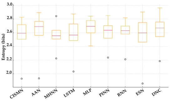
Figure 4.
Distributions of IG entropy across nine models.
In the following, we analyze each model’s attribution complexity by measuring the dispersion of feature-importance scores using Integrated Gradients entropy. This assessment highlights how chaotic and deterministic architectures compare in their interpretability, with a focused discussion on CISMN-5’s behavior and its implications for model explainability.
- Mid-Range Entropy: CISMN-5’s mean IG entropy of 2.58 bits places it squarely in the mid-range of all nine architectures. Although its chaotic memory, plasticity, synapse, and attention components diffuse feature-importance scores, they do not do so more severely than other nonlinear models such as PINN-3 (2.61 bits) or RNN-1 (2.61 bits). Despite its inherent nonlinear dynamics, the modest standard deviation (0.18 bits) indicates that CISMN-5 produces consistently stable attribution distributions across diverse test samples.
- Comparative Interpretability: Deterministic networks like MLP-2 (2.68 bits) and AAN-5 (2.64 bits) yield even higher mean entropy, signifying more diffuse and less interpretable attributions. In contrast, MHNN-1 achieves the lowest mean entropy (2.56 bits), suggesting that simpler, more constrained synaptic mechanisms can sometimes sharpen explanations.
- Variability and Flexibility: CISMN-5’s entropy range (1.93–2.83 bits) spans nearly the full spectrum observed, demonstrating its capacity to produce focused and dispersed explanations depending on the input. This adaptability arises from the dynamic interplay of multiple chaotic modules, which tailor feature importance in real time.
- Implications and Future Directions: These findings confirm that the CISMN’s multi-component chaotic updates complicate—but do not uniquely impair—the interpretability compared with other nonlinear architectures. Future CISMN variants will explore the targeted regularization of chaotic layers and surrogate attribution techniques to enhance the explanation clarity while preserving the model’s robust performance.
4. Discussion: In-Depth Comparison: CISMN vs. Traditional CHNNs
The CISMN departs fundamentally from prior chaotic neural network designs by weaving chaos theory into every significant component of the architecture. Rather than grafting chaotic activation functions or feedback loops onto otherwise deterministic models, the CISMN deliberately embeds logistic-map dynamics into its memory, plasticity, synaptic elements, attention, and optimization mechanisms. This orchestrated the use of bounded chaos which enhances the network’s ability to explore complex loss landscapes. It preserves stability and long-term dependency, overcoming the brittleness and training instability that have dogged traditional CHNN approaches.
At the heart of the CISMN lies a quartet of chaos-driven modules. Chaotic Memory Cells eschew fixed gating by blending 70% of each state update from the logistic map with 30% of the previous state, ensuring that a past context is neither lost nor allowed to dominate. Chaotic Plasticity Layers go beyond mere chaotic activation by injecting logistic-map perturbations directly into synaptic updates, enabling the network to escape poor local minima more effectively than a pure gradient descent. Chaotic Synapse Layers continuously adjust connection strengths through real-time chaotic feedback, mimicking the stochastic resonance of biological synapses. In contrast, Chaotic Attention replaces static softmax weighting with non-repeating logistic oscillations that adaptively prioritize features. Finally, a Chaotic Learning Rate Schedule governed by the logistic map (with a lower bound of η ≥ 10⁻⁶) introduces controlled randomness into optimization, further reducing entrapment in narrow minima.
In contrast, traditional CHNNs typically apply chaos only in isolated elements—most often within activation functions or ad–hoc feedback loops—while leaving gates, synaptic updates, and learning rates deterministic. They rely on fixed LSTM/GRU gates or simple recurrences for memory, standard backpropagation for weight updates, static or Hebbian synapses, and handcrafted or adaptive but deterministic learning-rate schedules. Crucially, they seldom incorporate explicit stabilization mechanisms to confine chaotic trajectories, often resulting in unstable training when pushed into highly nonlinear regimes. These architectural distinctions are summarized in Table 8.
Table 8.
Architectural distinctions of CISMN from traditional CHNNs.
By systematically embedding chaos across these modules and controlling sensitivity through empirically tuned blending ratios and bounded logistic-map parameters, the CISMN achieves a state-of-the-art performance on synthetic acoustical and real-world sonar regression tasks while maintaining stable, reproducible training runs. This contrasts sharply with traditional CHNNs’ tendency toward overdamped dynamics that fail to escape local minima or unbounded chaos, destabilizing learning.
5. Conclusions
We have presented the CISMN, a novel deep-learning architecture that elevates chaos theory from a peripheral concept to a core design principle. By embedding four dedicated chaotic modules—Chaotic Memory Cells, Chaotic Plasticity Layers, Chaotic Synapse Layers, and a Chaotic Attention Mechanism—alongside a logistic-map-driven learning-rate schedule, the CISMN systematically leverages the sensitivity dependence and ergodic properties of chaos to the following:
- Enhance the exploration of non-convex loss landscapes, allowing the model to escape local minima through controlled stochastic perturbations;
- Preserve long-term dependencies, as logistic-map-based memory updates maintain gradient magnitudes and avoid vanishing/exploding behaviors;
- Adapt feature prioritization in real time, via chaotic oscillations that dynamically adjust attention weights to suppress noise and amplify salient patterns.
Extensive experiments on two challenging regression benchmarks validate the CISMN’s effectiveness. On a synthetic acoustical dataset (541 samples, 22 features), CISMN-1 achieved an R2 = 0.791 and RMSE = 0.059, outperforming physics-informed networks and attention-augmented baselines. For the real-world PMLB sonar dataset (208 samples, 60 bands), CISMN-4 reached an R2 = 0.424 and RMSE = 0.380, substantially surpassing LSTM, memristive, and reservoir-based methods. Moreover, a five-fold cross-validation across seven standard regression problems (e.g., Diabetes, Boston Housing, Ames Housing) demonstrated that the CISMN not only matches, but often exceeds the performance of conventional and memory-augmented architectures, particularly in low-sample-to-feature regimes. Ablation and sensitivity studies further reveal a flexible scalability–efficiency trade-off: lightweight variants train under 10 s with competitive accuracy (e.g., CISMN-5 5 retains 96% of peak R2), while deeper configurations deliver marginal gains at a modest additional cost. Gradient-norm analyses confirm that chaotic state updates maintain backpropagation signals—the CISMN’s mean gradient norm remains in the thousands versus LSTM’s collapse to single digits, thus effectively circumventing vanishing-gradient issues. Rigorous reproducibility was ensured via fixed random seeds, constrained initialization ranges, and deterministic training protocols, yielding less than 1.2% relative variation across 20 independent runs. Despite these advances, the CISMN’s multi-component chaotic dynamics introduce interpretability challenges: feature-attribution entropies remain in the mid-range compared to other nonlinear models, indicating more dispersed importance scores. Future work will explore hybrid attribution techniques (e.g., surrogate modeling combined with Integrated Gradients), the targeted regularization of chaotic layers, and hardware-accelerated implementations (GPU-optimized logistic maps, FPGA-based chaotic units) to reduce computational overhead without sacrificing robustness.
The CISMN establishes a reproducible, modular framework for harnessing chaos as a computational asset rather than noise. Its demonstrated superiority in synthetic and real-world nonlinear regression tasks—combined with its adaptability, gradient stability, and reproducibility—positions it as a promising foundation for applications in financial forecasting, biomedical signal processing, environmental monitoring, and real-time control in autonomous systems. By treating controlled chaos as an integral design element, the CISMN paves the way for the next generation of deep-learning models capable of thriving amid the unpredictability of complex, non-stationary environments.
Author Contributions
All the authors contributed to the conception and design of this study. Y.S.: administration, conceptualization, supervision, methodology analysis, formal analysis, writing—review and editing. M.M.K.: Conceptualization, data curation, software, validation, methodology, investigation, writing—original draft. A.G.: Administration, conceptualization, supervision, formal analysis, writing—original draft, writing—review and editing. M.F. and S.P.: Supervision, formal analysis, writing, review and editing. All authors have read and agreed to the published version of the manuscript.
Funding
This research received no external funding.
Institutional Review Board Statement
This article is derived from a doctoral dissertation entitled "Development of a Machine Learning Model for Architectural Space Form-Finding with an Acoustic Optimization Approach," conducted under the supervision of Prof. Abbas Ghaffari, Dr. Yaser Shahbazi, Dr. Siamak Pedrammehr and Dr. Mohammad Fotouhi at the Tabriz Islamic Art University.
Data Availability Statement
The datasets generated and analyzed during the current study are publicly available and can be accessed via the following GitHub repository: https://github.com/archmohsen1991/CISMN-Source, accessed on 20 October 2024. As described in this paper, these datasets are part of the case studies that compare the CISMN model with other machine learning models. Also, the code developed for this study, titled “Chaos-Integrated Synaptic-Memory Network (CISMN)”, is publicly available on GitHub and can be accessed at https://github.com/archmohsen1991/CISMN-Source.
Conflicts of Interest
The authors declare no conflicts of interest.
References
- Shahbazi, Y.; Abdkarimi, M.; Ahmadnejad, F.; Kashavar, M.M.; Fotouhi, M.; Pedrammehr, S. Comparative Study of Optimal Flat Double-Layer Space Structures with Diverse Geometries through Genetic Algorithm. Buildings 2024, 14, 2816. [Google Scholar] [CrossRef]
- Ghaffari, A.; Shahbazi, Y.; Mokhtari Kashavar, M.; Fotouhi, M.; Pedrammehr, S. Advanced Predictive Structural Health Monitoring in High-Rise Buildings Using Recurrent Neural Networks. Buildings 2024, 14, 3261. [Google Scholar] [CrossRef]
- Safaei, M.; Hejazian, M.; Pedrammehr, S.; Pakzad, S.; Ettefagh, M.M.; Fotouhi, M. Damage Detection of Gantry Crane with a Moving Mass Using Artificial Neural Network. Buildings 2024, 14, 458. [Google Scholar] [CrossRef]
- Du, K.-L.; Swamy, M.N.S. Neural Networks and Statistical Learning; Springer: London, UK, 2014. [Google Scholar]
- Han, J.; Kamber, M.; Pei, J. Data Mining: Concepts and Techniques, 3rd ed.; Elsevier: Amsterdam, The Netherlands, 2011. [Google Scholar]
- Haykin, S.S. Neural Networks and Learning Machines, 3rd ed.; Pearson Education: London, UK, 2009. [Google Scholar]
- Hinton, G.E.; Osindero, S.; Teh, Y.-W. A Fast Learning Algorithm for Deep Belief Nets. Neural Comput. 2006, 18, 1527–1554. [Google Scholar] [CrossRef]
- Sarker, I.H. Deep Learning: A Comprehensive Overview on Techniques, Taxonomy, Applications and Research Directions. SN Comput. Sci. 2021, 2, 420. [Google Scholar] [CrossRef]
- Al-Musawi, W.A.; Wali, A.W.; Abd Ali Al-Ibadi, M. New artificial neural network design for Chua chaotic system prediction using FPGA hardware co-simulation. Int. J. Electr. Comput. Eng. (IJECE) 2022, 12, 1955. [Google Scholar] [CrossRef]
- Javanshir, A.; Nguyen, T.T.; Mahmud, M.A.P.; Kouzani, A.Z. Advancements in Algorithms and Neuromorphic Hardware for Spiking Neural Networks. Neural Comput. 2022, 34, 1289–1328. [Google Scholar] [CrossRef]
- Churchill, V.; Xiu, D. Deep Learning of Chaotic Systems from Partially-Observed Data. arXiv 2022, arXiv:2205.08384. [Google Scholar] [CrossRef]
- Karhunen, J.; Raiko, T.; Cho, K. Unsupervised deep learning. In Advances in Independent Component Analysis and Learning Machines; Elsevier: Amsterdam, The Netherlands, 2015; pp. 125–142. [Google Scholar]
- Lin, H.; Wang, C.; Yu, F.; Sun, J.; Du, S.; Deng, Z.; Deng, Q. A Review of Chaotic Systems Based on Memristive Hopfield Neural Networks. Mathematics 2023, 11, 1369. [Google Scholar] [CrossRef]
- Zhou, B.; Xu, N. Transient Chaotic Neural Networks Based on Sinusoidal Feedback Terms and Their Applications. In Proceedings of the 2023 4th International Conference on Electronic Communication and Artificial Intelligence (ICECAI), Guangzhou, China, 12–14 May 2023; pp. 343–347. [Google Scholar]
- Clark, D.G.; Abbott, L.F. Theory of Coupled Neuronal-Synaptic Dynamics. Phys. Rev. X 2024, 14, 021001. [Google Scholar] [CrossRef]
- Du, W.; Huang, H. Synaptic plasticity alters the nature of chaos transition in neural networks. arXiv 2024, arXiv:2412.15592. [Google Scholar]
- Shao, L.; Zhao, Y.; Liu, Y. Organic Synaptic Transistors: The Evolutionary Path from Memory Cells to the Application of Artificial Neural Networks. Adv. Funct. Mater. 2021, 31, 2101951. [Google Scholar] [CrossRef]
- Talsma, W.; van Loo, H.; Shao, S.; Jung, S.; Allard, S.; Scherf, U.; Loi, M.A. Synaptic Plasticity in Semiconducting Single-Walled Carbon Nanotubes Transistors. Adv. Intell. Syst. 2020, 2, 2000154. [Google Scholar] [CrossRef]
- Huang, W.; Li, Y.; Huang, Y. Deep Hybrid Neural Network and Improved Differential Neuroevolution for Chaotic Time Series Prediction. IEEE Access 2020, 8, 159552–159565. [Google Scholar] [CrossRef]
- Xu, B.; Geng, H.; Yin, Y.; Li, P. DISTA: Denoising Spiking Transformer with intrinsic plasticity and spatiotemporal attention. arXiv 2023, arXiv:2311.09376. [Google Scholar]
- Novelli, N.; Belardinelli, P.; Lenci, S. Piecewise integrable neural network: An interpretable chaos identification framework. Chaos Interdiscip. J. Nonlinear Sci. 2023, 33, 023107. [Google Scholar] [CrossRef]
- Zhang, F.; Chen, L.; Kou, L.; Hu, Z.; Shu, M.; Wang, G. Chaotic neural networks with complex-valued weight and its applications in electrocardiogram classification. Phys. Scr. 2024, 99, 015240. [Google Scholar] [CrossRef]
- Gao, Z.; Zhang, D.; Zhu, S. Hybrid event-triggered synchronization control of delayed chaotic neural networks against communication delay and random data loss. Chaos Solitons Fractals 2023, 172, 113535. [Google Scholar] [CrossRef]
- Lai, Q.; Lai, C.; Kuate, P.D.K.; Li, C.; He, S. Chaos in a Simplest Cyclic Memristive Neural Network. Int. J. Bifurc. Chaos 2022, 32, 22500420. [Google Scholar] [CrossRef]
- Baby, H.; Raghu, M. Chaotic neural network for information security. e-Prime—Adv. Electr. Eng. Electron. Energy 2024, 8, 100524. [Google Scholar] [CrossRef]
- Lephalala, M.; Vives, S.S.; Bisetty, K. Chaotic neural network algorithm with competitive learning integrated with partial Least Square models for predicting the toxicity of fragrances in sanitizers and disinfectants. Sci. Total Environ. 2024, 942, 173754. [Google Scholar] [CrossRef] [PubMed]
- Osama, A.; Gadallah, S.I.; Said, L.A.; Radwan, A.G.; Fouda, M.E. Chaotic neural network quantization and its robustness against adversarial attacks. Knowl. Based Syst. 2024, 286, 111319. [Google Scholar] [CrossRef]
- Ruan, Z.; Mei, J.; Li, Y.; Duan, S.; Wang, L. Exponential synchronization of uncertain chaotic inertial neural networks by guaranteed cost intermittent control. Neurocomputing 2024, 570, 127049. [Google Scholar] [CrossRef]
- Anzo-Hernández, A.; Zambrano-Serrano, E.; Platas-Garza, M.A.; Volos, C. Dynamic Analysis and FPGA Implementation of Fractional-Order Hopfield Networks with Memristive Synapse. Fractal Fract. 2024, 8, 628. [Google Scholar] [CrossRef]
- Ding, S.; Wang, N.; Bao, H.; Chen, B.; Wu, H.; Xu, Q. Memristor synapse-coupled piecewise-linear simplified Hopfield neural network: Dynamics analysis and circuit implementation. Chaos Solitons Fractals 2023, 166, 112899. [Google Scholar] [CrossRef]
- Bao, H.; Chen, Z.; Chen, M.; Xu, Q.; Bao, B. Memristive-cyclic Hopfield neural network: Spatial multi-scroll chaotic attractors and spatial initial-offset coexisting behaviors. Nonlinear Dyn. 2023, 111, 22535–22550. [Google Scholar] [CrossRef]
- Liu, D.; Cao, Y.; Mou, J.; Alharbi khalid, H. Dynamical analysis and DSP implementation of discrete memristor coupled discrete bi-neuron Hopfield neural networks. Phys. Scr. 2025. [Google Scholar] [CrossRef]
- Mahdavi, N.; Menhaj, M.B. A new set of sufficient conditions based on coupling parameters for synchronization of Hopfield like Chaotic Neural Networks. Int. J. Control Autom. Syst. 2011, 9, 104–111. [Google Scholar] [CrossRef]
- Zhang, S.; Li, Y.; Lu, D.; Li, C. A novel memristive synapse-coupled ring neural network with countless attractors and its application. Chaos Solitons Fractals 2024, 184, 115056. [Google Scholar] [CrossRef]
- Chen, C.; Bao, H.; Chen, M.; Xu, Q.; Bao, B. Non-ideal memristor synapse-coupled bi-neuron Hopfield neural network: Numerical simulations and breadboard experiments. AEU—Int. J. Electron. Commun. 2019, 111, 152894. [Google Scholar] [CrossRef]
- Chen, M.; Chen, C.; Bao, B.; Xu, Q. Multi-stable patterns coexisting in memristor synapse-coupled Hopfield neural network. In Mem-Elements for Neuromorphic Circuits with Artificial Intelligence Applications; Elsevier: Amsterdam, The Netherlands, 2021; pp. 439–459. [Google Scholar]
- Zhiyuan, F.; Yan, L.; Guangyi, W.; Yana, G. Memristive discrete chaotic neural network and its application in associative memory. Analog. Integr. Circuits Signal Process 2024, 118, 329–342. [Google Scholar] [CrossRef]
- Ramakrishnan, B.; Wang, Z.; Natiq, H.; Pal, N.; Rajagopal, K.; Jafari, S. Dynamics of a two-neuron hopfield neural network: Memristive synapse and autapses and impact of fractional order. AEU—Int. J. Electron. Commun. 2024, 187, 155506. [Google Scholar] [CrossRef]
- Yang, N.; Liang, J.; Wu, C.; Guo, Z. Dynamics and Implementation of FPGA for Memristor-Coupled Fractional-Order Hopfield Neural Networks. Int. J. Bifurc. Chaos 2024, 34, 2450106. [Google Scholar] [CrossRef]
- Ding, D.; Xiao, H.; Yang, Z.; Luo, H.; Hu, Y.; Zhang, X.; Liu, Y. Coexisting multi-stability of Hopfield neural network based on coupled fractional-order locally active memristor and its application in image encryption. Nonlinear Dyn. 2022, 108, 4433–4458. [Google Scholar] [CrossRef]
- Dai, Z.W.; Wei, D.Q. Dynamical behavior of memristive Hopfield neural network under pulsed current excitation. Phys. Lett. A 2024, 522, 129789. [Google Scholar] [CrossRef]
- Lin, H.; Wang, C.; Sun, Y.; Wang, T. Generating n-Scroll Chaotic Attractors From a Memristor-Based Magnetized Hopfield Neural Network. IEEE Trans. Circuits Syst. II Express Briefs 2023, 70, 311–315. [Google Scholar] [CrossRef]
- Li, X.; He, Q.; Yu, T.; Cai, Z.; Xu, G. Coexistence behavior of asymmetric attractors in hyperbolic-type memristive Hopfield neural network and its application in image encryption. Chin. Phys. B 2024, 33, 030505. [Google Scholar] [CrossRef]
- Min, F.; Chen, C.; Broderick, N.G.R. Coupled Homogeneous Hopfield Neural Networks: Simplest Model Design, Synchronization, and Multiplierless Circuit Implementation. IEEE Trans. Neural Netw. Learn. Syst. 2025, 4, 1–8. [Google Scholar] [CrossRef]
- Aghaei, A. Chaotic Dynamics of a Two-Neuron Memristive Hopfield Neural Network under Electromagnetic Radiation. Asian J. Res. Comput. Sci. 2024, 17, 89–107. [Google Scholar] [CrossRef]
- Hochreiter, S.; Schmidhuber, J. Long Short-Term Memory. Neural Comput. 1997, 9, 1735–1780. [Google Scholar] [CrossRef]
- Vaswani, A.; Shazeer, N.; Parmar, N.; Uszkoreit, J.; Jones, L.; Gomez, A.N.; Kaiser, Ł. Attention Is All You Need. In International Conference on Neural Information Processing Systems; Luxburg, V.L., Guyon, I., Bengio, S., Eds.; Curran Associates Inc: Long Beach, CA, USA, 2017. [Google Scholar]
- Fournier, S.J.; Urbani, P. Statistical physics of learning in high-dimensional chaotic systems. J. Stat. Mech. Theory Exp. 2023, 2023, 113301. [Google Scholar] [CrossRef]
- Barrio, R.; Lozano, Á.; Mayora-Cebollero, A.; Mayora-Cebollero, C.; Miguel, A.; Ortega, A.; Serrano, S.; Vigara, R. Deep Learning for chaos detection. Chaos Interdiscip. J. Nonlinear Sci. 2023, 33, 073146. [Google Scholar] [CrossRef] [PubMed]
- Ke, Q.; Oommen, B.J. Logistic Neural Networks: Their chaotic and pattern recognition properties. Neurocomputing 2014, 125, 184–194. [Google Scholar] [CrossRef]
- Bishop, C.M. Pattern Recognition and Machine Learning (Information Science and Statistics), 1st ed.; Springer: Berlin/Heidelberg, Germany, 2007. [Google Scholar]
- Strogatz, S.H. Nonlinear Dynamics And Chaos: With Applications To Physics, Biology, Chemistry, And Engineering (Studies in Nonlinearity), 1st ed.; CRC Press: Boca Raton, FL, USA, 2024. [Google Scholar]
- May, R.M. Simple mathematical models with complicated dynamics. Nature 1976, 261, 459–467. [Google Scholar] [CrossRef]
- Cho, K.; van Merrienboer, B.; Gulcehre, C.; Bahdanau, D.; Bougares, F.; Schwenk, H.; Bengio, Y. Learning Phrase Representations using RNN Encoder-Decoder for Statistical Machine Translation. arXiv 2014. [Google Scholar] [CrossRef]
- Kaneko, K. Coupled Map Lattice. In Chaos, Order, and Patterns; Artuso, R., Casati, G., Cvitanović, P., Eds.; Springer: Boston, MA, USA, 1991; pp. 237–247. [Google Scholar] [CrossRef]
- Ott, E. Chaos in Dynamical Systems; Cambridge University Press: Cambridge, UK, 2002. [Google Scholar]
- Uhl-Bien, M.; Piccolo, R.F.; Schermerhorn, J.R., Jr. Organizational Behavior, 2nd ed.; Wiley: Hoboken, NJ, USA, 2020. [Google Scholar]
- Risken, H. The Fokker-Planck Equation; Springer: Berlin/Heidelberg, Germany, 1996. [Google Scholar]
- Lasota, A.; Mackey, M.C. Chaos, Fractals, and Noise; Springer: New York, NY, USA, 1994. [Google Scholar]
- West, B. Fractional Calculus View of Complexity: Tomorrow’s Science; MIT Press: Cambridge, MA, USA, 2015. [Google Scholar]
- Pusuluri, K.; Ju, H.; Shilnikov, A. Chaotic Dynamics in Neural Systems. In Encyclopedia of Complexity and Systems. In Encyclopedia of Complexity and Systems Science; Springer: Berlin/Heidelberg, Germany, 2020; pp. 1–13. [Google Scholar]
- Goodfellow, I.; Bengio, Y.; Courville, A. Deep Learning, 1st ed.; The MIT Press: Cambridge, MA, USA, 2016. [Google Scholar]
- Jiang, Z.; Chen, Z.; Hou, T.; Huang, H. Spectrum of non-Hermitian deep-Hebbian neural networks. Phys. Rev. Res. 2023, 5, 013090. [Google Scholar] [CrossRef]
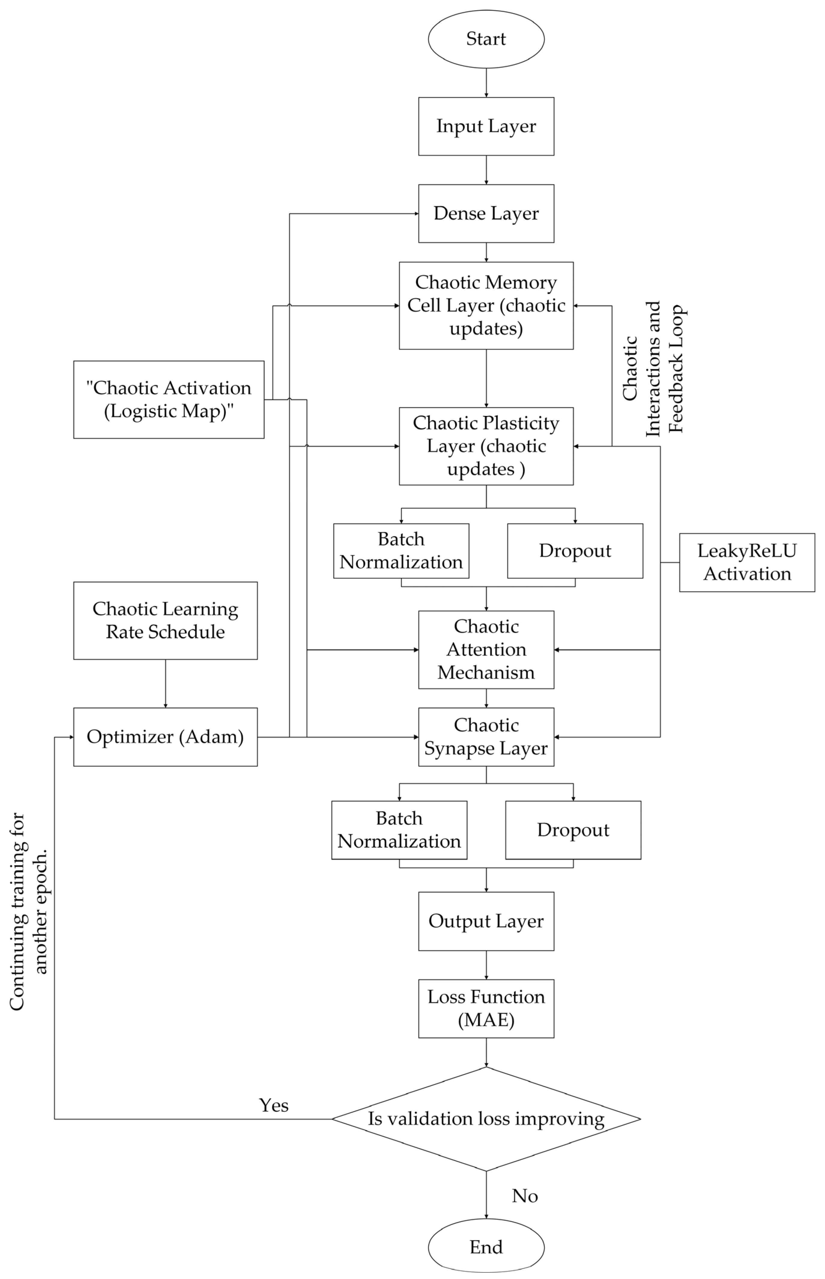
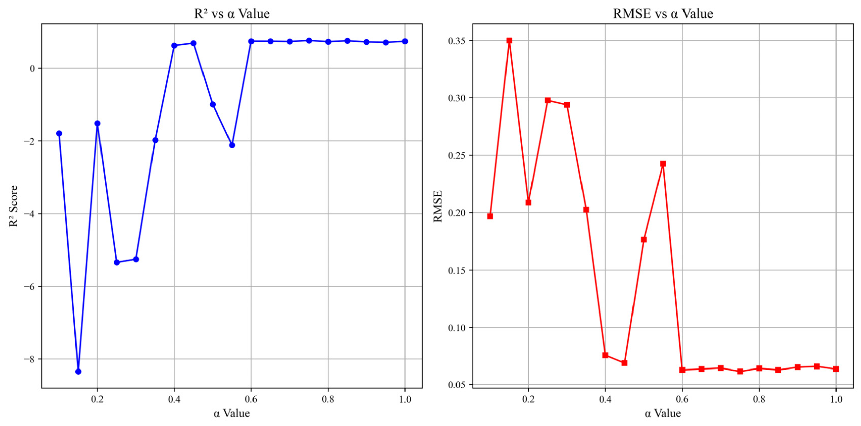
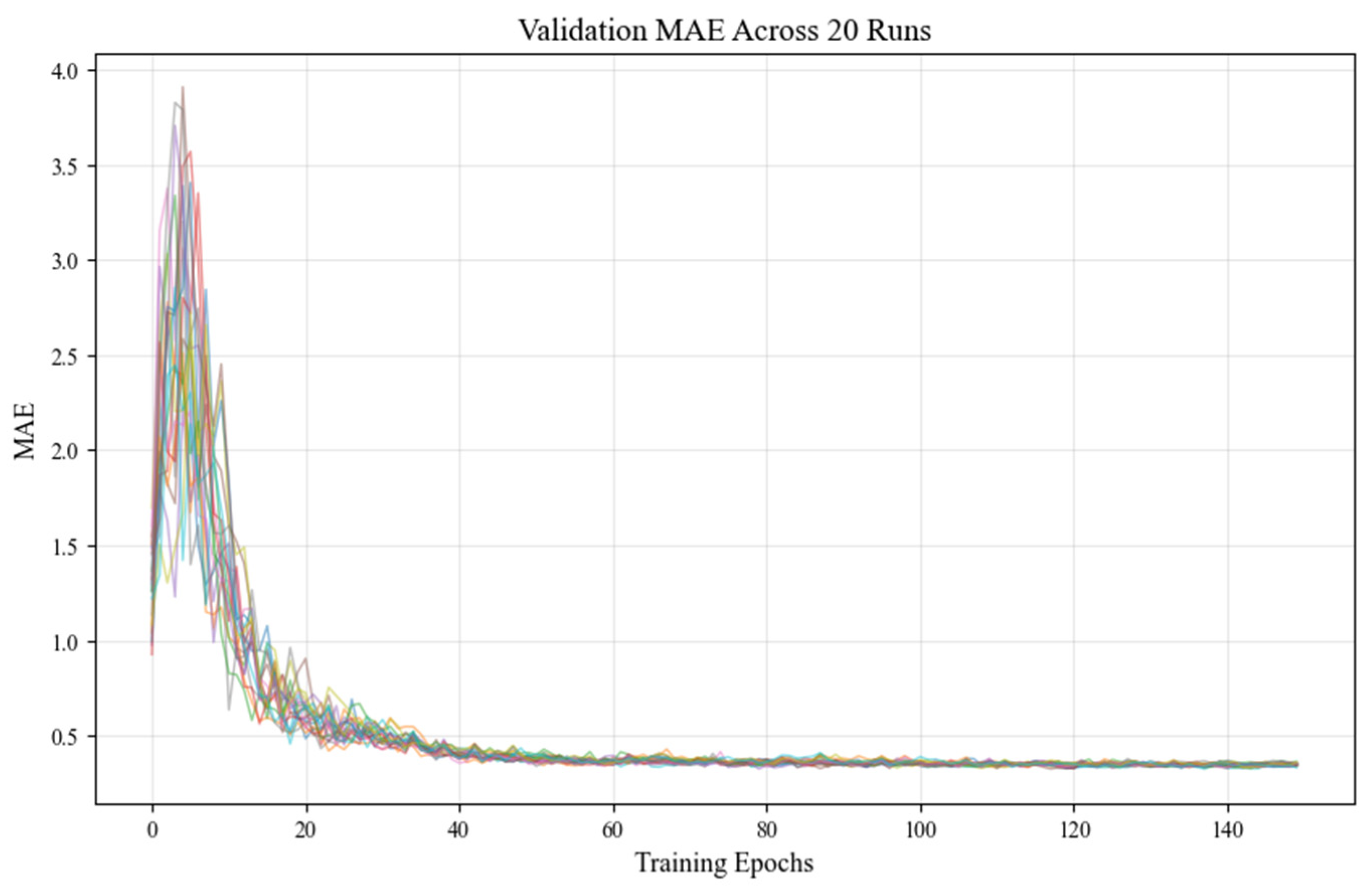
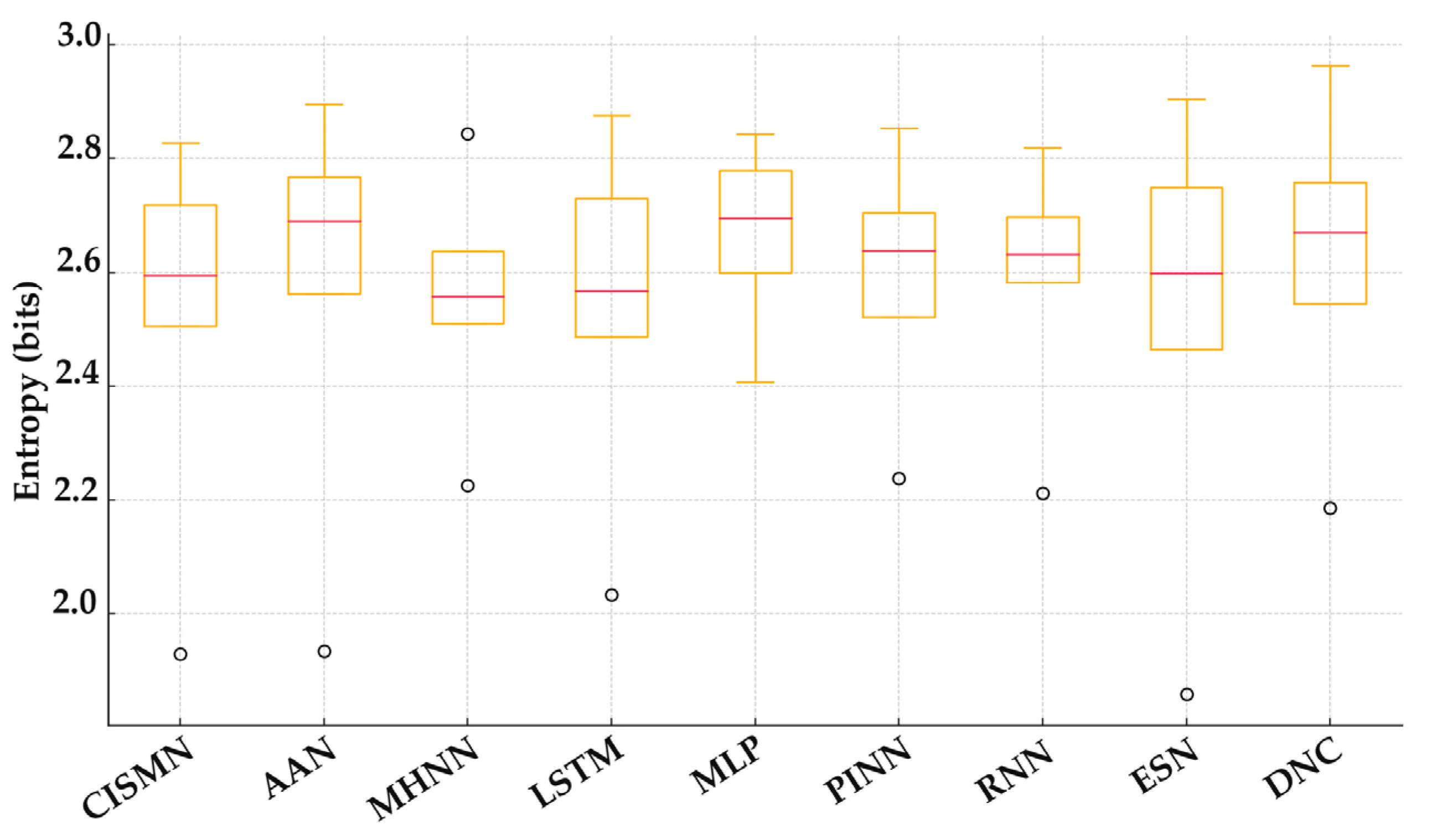
Disclaimer/Publisher’s Note: The statements, opinions and data contained in all publications are solely those of the individual author(s) and contributor(s) and not of MDPI and/or the editor(s). MDPI and/or the editor(s) disclaim responsibility for any injury to people or property resulting from any ideas, methods, instructions or products referred to in the content. |
© 2025 by the authors. Licensee MDPI, Basel, Switzerland. This article is an open access article distributed under the terms and conditions of the Creative Commons Attribution (CC BY) license (https://creativecommons.org/licenses/by/4.0/).